跳到论文正文
W Papers独立论文阅读器 arXiv:2404.16642 论文正文 计算阅读时间 · 0%
引用这篇论文根据当前论文元数据生成,正式投稿前建议核对。


\indexsetup

level=

,

Nathanaël Berestycki    Ellen Powell

noclearpage [title=Index] [name=notation,title=Notation and Symbols,columns=2]

Gaussian free field
and Liouville quantum gravity

Nathanaël Berestycki    Ellen Powell
[Uncaptioned image]

A book based on this material will be published by Cambridge University Press. This version is free to view and download for personal use only. Not for re-distribution, re-sale or use in derivative works.

©Nathanaël Berestycki and Ellen Powell, 2024.

For our families

Preface

Over fourty years ago, the physicist Polyakov [Pol81] proposed a bold framework for string theory, in which the problem was reduced to the study of certain “random surfaces”. He further made the tantalising suggestion that this theory could be explicitly solved.

Recent breakthroughs from the last fifteen years such as (among many other works) [DKRV16, KRV20, DS11, DMS21, MS20, HS23, LG13, Mie13, GM21c, DDDF20, GM21d, GM21b, BGK+24] have not only given a concrete mathematical basis for this theory but also verified some of its most striking predictions – as well as Polyakov’s original vision. This theory, now known in the mathematics literature either as Liouville quantum gravity (LQG) or Liouville conformal field theory (CFT), is based on a remarkable combination of ideas coming from different fields, above all probability and geometry. At its heart is the planar Gaussian free field (GFF) hℎh, a random distribution on a given reference surface or domain of ℝ2superscriptℝ2\mathbb{R}^{2} whose covariance involves the Green function. A key role is played by the family of measures ℳγsuperscriptℳ𝛾\mathcal{M}^{\gamma} (sometimes referred to as Liouville measures, although this should not be confused with the notion of Liouville measure arising for instance in Hamiltonian dynamics) defined formally as ℳγ​(d⁡x)=exp⁡(γ​h​(x))​d⁡xsuperscriptℳ𝛾d𝑥𝛾ℎ𝑥d𝑥\mathcal{M}^{\gamma}(\operatorname{d\!}x)=\exp(\gamma h(x))\operatorname{d\!}x, for a parameter γ𝛾\gamma known as the coupling constant.

This book is intended to be an introduction to these developments assuming as few prerequisites as possible. Our starting point is a self-contained and thorough introduction to the two-dimensional continuum Gaussian free field (GFF). Although surveys and overviews of this object have been written before (notably [She07, WP21]), which give plenty of context, both historical and in relation to other topics, the presentation here gives a comprehensive and systematic treatment of some of the analytic subtleties that arise. Many of the details given here for the construction and basic properties of the GFF have perhaps surprisingly not appeared anywhere else before, to the best of our knowledge.

The second basic ingredient and main building block for subsequent chapters is the theory of Gaussian multiplicative chaos. Historically, this theory was first proposed by Høegh-Krohn in [HK71] with motivations from constructive quantum field theory not too dissimilar from the ones of this book. In the mathematical literature however it was Kahane, in his seminal contribution [Kah85], who introduced it, independently of (and going considerably beyond) [HK71]. Kahane was for his part initially motivated by the description of turbulence. In addition to these two distinct motivations, the theory has since found numerous applications in seemingly unrelated areas, such as random matrices, number theory, mathematical finance and planar Brownian motion. A useful and early survey of this theory was written in [RV14] which sketched some of the arguments of the best results available at the time, and also outlined some of these applications. However the state of the art has evolved considerably since then; as a result ours is probably the first unified, systematic and self-contained presentation of this theory.

With these tools in hand, the second part of our book is devoted to an exposition of some aspects of Liouville quantum gravity as well as Liouville conformal field theory. These two topics are closely related to one another and they describe, roughly speaking, the same physical theory but with somewhat different perspectives. Essentially, we use the label “Liouville quantum gravity” for a random geometric approach highlighting connections with Schramm–Loewner Evolution (SLE). By contrast, we use the label “Liouville conformal field theory” for an approach based on the path integral formulation. We cover topics such as correlation functions and the so-called Seiberg bounds, Weyl anomaly formula, quantum cones and wedges, quantum zipper, and mating of trees, as well as discrete counterparts to this theory in the form of random planar maps decorated by a model of statistical mechanics (namely, the self-dual Fortuin–Kasteleyn percolation model).

These developments require us to work with variants of the (Dirichlet) GFF, respectively the GFF on a Riemannian surface and GFF with Neumann boundary conditions, to which we also provide a systematic introduction. In fact, to the best of our knowledge this is the first place where the analytic details of their construction are given in full.

More specifically, the topics covered include:

  • •

    Chapter 1: the definition and main properties of the GFF with Dirichlet (or zero) boundary conditions;

  • •

    Chapter 2: the construction of the Liouville measure (in the GFF case), its non degeneracy and change of coordinate formula;

  • •

    Chapter 3: a comprehensive exposition of the construction and properties of general Gaussian multiplicative chaos measures;

  • •

    Chapter 4: an introduction to statistical mechanics on random planar maps – the discrete counterparts of Liouville quantum gravity – and Sheffield’s bijection with pairs of trees [She16b];

  • •

    Chapter 5: an introduction to Liouville conformal field theory, as developed in a series of papers starting with [DKRV16] by David, Kupiainen, Rhodes and Vargas;

  • •

    Chapter 6: the definition, construction and main properties of the GFF with Neumann boundary conditions;

  • •

    Chapter 7: an account of the notion of quantum surfaces, and the theory of special quantum surfaces enjoying scale invariance, such as quantum spheres, discs, wedges and cones; and a proof of equivalence with aspects of the theory developed in Chapter 5;

  • •

    Chapter 8: an exposition of Sheffield’s quantum zipper theorem (with novel additional details) and its relation with conformal welding [She16a];

  • •

    Chapter 9: an introduction to the powerful mating-of-trees theory of Duplantier, Miller and Sheffield [DMS21]. This includes an extensive and partly novel treatment of space-filling and whole-plane SLE.

The final three topics above are rather technical, and readers are advised that it will be of most use to people who are actively working in this area. See also Figure 1 for a reading guide.

Refer to caption
Figure 1: Guide to reading. A solid arrow from Chapter m𝑚m to Chapter n𝑛n indicates that m𝑚m is a preqrequisite for n𝑛n. A dashed arrow indicates a complementary perspective on similar/related topics. The ≃similar-to-or-equals\simeq symbol indicates that Chapter 2 and Chapter 3 are somewhat parallel, with Chapter 2 being focused solely on the construction of the Gaussian Multiplicative Chaos (GMC) measure associated to the (Dirichlet) Gaussian free field, while Chapter 3 gives an exposition of the general theory of GMC.

The theory is in full blossom and attempting to make a complete survey of the field would be hopeless, so quickly is it developing. Nevertheless, as the theory grows in complexity and applicability, it has appeared useful to summarise some of its basic and foundational aspects in one place, especially since complete proofs of some facts can be spread over a multitude of papers.

Clearly, the main drawback of this approach is that many of the important subsequent developments and alternative points of view are not included. For instance: the expansive body of work on random planar maps and their rigorous connections with Liouville quantum gravity, the Brownian map, Liouville Brownian motion, imaginary geometry, imaginary chaos, and the Liouville quantum gravity metric, do not feature in this book. For all this we apologise in advance.

Acknowledgements

An initial draft was written by the first-named author, in preparation for the LMS / Clay institute research school on Modern Developments in Probability taking place in Oxford, July 2015. The draft was subsequently revised on the occasion of several courses given on this material: at the Spring School on Geometric Models in Probability in Darmstadt, then in July 2016 for the Probability Summer School at Northwestern (for which the chapter on statistical physics on random planar maps was added), in December 2017 for the Lectures on Probability and Statistics (LPS) at ISI Kolkata, and in Berlin at the Stochastic Analysis in Interaction summer school, in 2023. The second-named author lectured on parts of this material in Helsinki in 2022, Santiago de Chile in 2023, and Guanajuato (CIMAT) in 2023.

In all cases we thank the organisers (Christina Goldschmidt and Dmitry Beliaev; Volker Betz and Matthias Meiners; Antonio Auffinger and Elton Hsu; Arijit Chakrabarty, Manjunath Krishnapur, Parthanil Roy and especially Rajat Subhra Hazra; Peter Friz and Peter Bank; Eero Saksman and Eveliina Peltola; Avelio Sepúlveda and Daniel Remenik; and Daniel Kious, Andreas Kyprianou, Sandra Palau and Juan Carlos Pardo) for their invitations and superb organisation. Thanks also to Benoit Laslier for agreeing to run the exercise sessions accompanying the lectures at the initial school.

The Isaac Newton institute’s semester on Random Geometry in 2015 was another important influence and motivation for this book, and we would like to thank the INI for its hospitality. In fact, this semester served as the second author’s initiation into the world of the Gaussian free field and Liouville quantum gravity. The resulting years of discussions between us has led to the present expanded and revised version. We would like to thank many of the INI programme participants for enlightening discussions related to aspects of the book; especially, Omer Angel, Juhan Aru, Stéphane Benoît, Bertrand Duplantier, Ewain Gwynne, Nina Holden, Henry Jackson, Benoit Laslier, Jason Miller, James Norris, Gourab Ray, Scott Sheffield, Xin Sun, Wendelin Werner and Ofer Zeitouni. Special thanks in particular to Juhan Aru, Ewain Gwynne, Nina Holden and Xin Sun for many inspiring discussions over the years over a broad range of topics.

We would also like to thank the participants of two reading groups at the University of Bonn and ETH Zürich/University of Zürich respectively (particularly the organisers Nina Holden and Eveliina Peltola) which followed these notes, and led to many helpful comments. We also received important feedback following graduate courses based on this material which took place at MIT, University of Washington and University of Vienna. Participants and organisers (Scott Sheffield and Zhen-Qing Chen) are warmly acknowledged. We would particularly like to thank Scott Sheffield for his constant encouragement throughout.

A substantial part of the writing took place while the authors were invited participants to the semester on The Analysis and Geometry of Random Spaces which took place at MSRI in 2022 (now Simons–Laufer Mathematical Sciences Institute) in Berkeley, California. We are very grateful to the organisers of the programme (Mario Bonk, Steffen Rohde, Joan Lind, Eero Saksman, Fredrik Viklund, Jang-Mei Wu) for this amazing opportunity. We also thank the many other participants of this programme for the pleasant atmosphere and the many comments we received while working on Chapter 5 of this book in connection with the reading group on Liouville CFT.

Finally, comments on versions of this draft have been received at various stages from Juhan Aru, Jacopo Borga, Zhen-Qing Chen, William Da Silva, Nina Holden, Henry Jackson, Jakob Klein, Aleksandra Korzhenkova, Benoit Laslier, Joona Oikarinen, Léonie Papon, Eveliina Peltola, Gourab Ray, Mark Sellke, Huy Tran, Joonas Turunen, Fredrik Viklund, Mo-Dick Wong, Henrik Weber and Dapeng Zhan. We are grateful for their input which helped to correct minor problems, as well as to emphasise some of the subtle aspects of the arguments. Of course we hasten to add that we retain the entire responsibility for any remaining typo, error, omission, or lack of clarity.

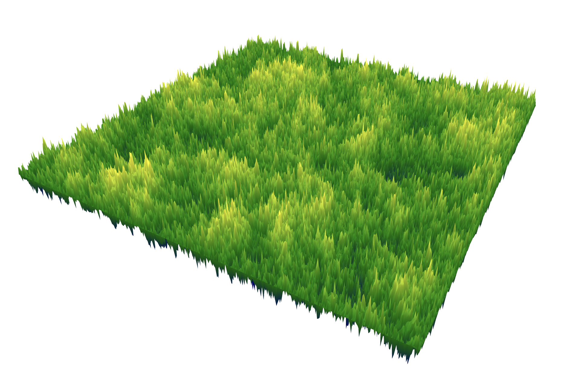
Thanks also to Jason Miller and to Jérémie Bettinelli and Benoit Laslier for letting us use some of their beautiful simulations which can be seen on the cover and in Chapter 4.

The work of the first author was supported during various stages of the writing by EPSRC (via grants EP/I03372X/1 and EP/L018896/1) and the FWF (via grant 10.55776/P33083), while the second author has been supported by the SNF grant 175505 and the UKRI Future Leader’s Fellowship MR/W008513/1. This support is gratefully acknowledged.

Nathanaël Berestycki

Ellen Powell

Vienna and Durham, February 2024

1 Definition and properties of the GFF

1.1 Discrete case

  The discrete case is included here only for the purpose of guiding intuition when we come to work in the continuum.  

Consider a finite, weighted, undirected graph 𝒢=(V,E)𝒢𝑉𝐸\mathcal{G}=(V,E) (with weights (we)e∈Esubscriptsubscript𝑤𝑒𝑒𝐸(w_{e})_{e\in E} on the edges). For instance, 𝒢𝒢\mathcal{G} could be a finite portion of the Euclidean lattice ℤdsuperscriptℤ𝑑\mathbb{Z}^{d} with weights we≡1subscript𝑤𝑒1w_{e}\equiv 1. Let ∂\partial be a distinguished set of vertices, called the boundary of the graph, and set V^=V∖∂^𝑉𝑉\hat{V}=V\setminus\partial. Let (Xt)t≥0subscriptsubscript𝑋𝑡𝑡0(X_{t})_{t\geq 0} be the random walk on 𝒢𝒢\mathcal{G} in continuous time, meaning that it jumps from x𝑥x to y𝑦y at rate wx,ysubscript𝑤𝑥𝑦w_{x,y}, and let τ𝜏\tau be the first time that X𝑋X hits ∂\partial (which we assume to be finite almost surely for every starting point).

Write Q=(qx,y)x,y∈V𝑄subscriptsubscript𝑞𝑥𝑦𝑥𝑦𝑉Q=(q_{x,y})_{x,y\in V} for the Q𝑄Q-matrix of X𝑋X. That is, its infinitesimal generator, so that for each x∈V𝑥𝑉x\in V, qx,y=wx,ysubscript𝑞𝑥𝑦subscript𝑤𝑥𝑦q_{x,y}=w_{x,y} for y≠x𝑦𝑥y\neq x and qx,x=−∑y∼xwx,y<∞subscript𝑞𝑥𝑥subscriptsimilar-to𝑦𝑥subscript𝑤𝑥𝑦q_{x,x}=-\sum_{y\sim x}w_{x,y}<\infty where y∼xsimilar-to𝑦𝑥y\sim x means that x𝑥x and y𝑦y are connected by an edge in E𝐸E. Note that the uniform measure π​(x)≡1𝜋𝑥1\pi(x)\equiv 1 is reversible for X𝑋X. We write ℙxsubscriptℙ𝑥\mathbb{P}_{x} for the law of the random walk started and x∈V𝑥𝑉x\in V and 𝔼xsubscript𝔼𝑥\mathbb{E}_{x} for the corresponding expectation.

Definition 1.1 (Green function).

The Green function G​(x,y)𝐺𝑥𝑦G(x,y) is defined for any x,y∈V𝑥𝑦𝑉x,y\in V by setting

G​(x,y)=𝔼x​(∫0∞𝟏{Xt=y;τ>t}​d⁡t).𝐺𝑥𝑦subscript𝔼𝑥superscriptsubscript0subscript1formulae-sequencesubscript𝑋𝑡𝑦𝜏𝑡d𝑡G(x,y)=\mathbb{E}_{x}\left(\int_{0}^{\infty}\mathbf{1}_{\{X_{t}=y;\tau>t\}}\operatorname{d\!}t\right).

In other words G​(x,y)𝐺𝑥𝑦G(x,y) is the expected time that X𝑋X spends at y𝑦y, when started from x𝑥x, before hitting the boundary. Note that with this definition we have G​(x,y)=G​(y,x)𝐺𝑥𝑦𝐺𝑦𝑥G(x,y)=G(y,x) for all x,y∈V^𝑥𝑦^𝑉x,y\in\hat{V}, since ℙx​(Xt=y;τ>t)=ℙy​(Xt=x;τ>t)subscriptℙ𝑥formulae-sequencesubscript𝑋𝑡𝑦𝜏𝑡subscriptℙ𝑦formulae-sequencesubscript𝑋𝑡𝑥𝜏𝑡\mathbb{P}_{x}(X_{t}=y;\,\tau>t)=\mathbb{P}_{y}(X_{t}=x;\,\tau>t) by reversibility of X𝑋X with respect to π𝜋\pi.

An equivalent expression for the Green function when working with the random walk in discrete time Y=(Yn)n≥0𝑌subscriptsubscript𝑌𝑛𝑛0Y=(Y_{n})_{n\geq 0} (which jumps from x𝑥x to y𝑦y with probability proportional to wx,ysubscript𝑤𝑥𝑦w_{x,y}) is

G​(x,y)=1qy​𝔼x​(∑n=0∞𝟏{Yn=y;τ​(Y)>n}),𝐺𝑥𝑦1subscript𝑞𝑦subscript𝔼𝑥superscriptsubscript𝑛0subscript1formulae-sequencesubscript𝑌𝑛𝑦𝜏𝑌𝑛G(x,y)=\frac{1}{q_{y}}\mathbb{E}_{x}\left(\sum_{n=0}^{\infty}\mathbf{1}_{\{Y_{n}=y;\tau(Y)>n\}}\right), (1.1)

where qy=∑y∼xwx,y=−qy,ysubscript𝑞𝑦subscriptsimilar-to𝑦𝑥subscript𝑤𝑥𝑦subscript𝑞𝑦𝑦q_{y}=\sum_{y\sim x}w_{x,y}=-q_{y,y} and τ​(Y)𝜏𝑌\tau(Y) is the first time that Y𝑌Y hits ∂D𝐷\partial D. Indeed, X𝑋X and Y𝑌Y can be coupled in such a way that for each y∈V^𝑦^𝑉y\in\hat{V} and each visit of Y𝑌Y to y𝑦y, X𝑋X stays at y𝑦y for an exponentially distributed time with mean 1/qy1subscript𝑞𝑦1/q_{y}.

The Green function is a basic ingredient in the definition of the Gaussian free field, so the following elementary properties will be important to us.

Proposition 1.2.

Let Q^^𝑄\hat{Q} denote the restriction of Q𝑄Q to V^×V^^𝑉^𝑉\hat{V}\times\hat{V}. Then

  1. 1.

    (−Q^)−1​(x,y)=G​(x,y)superscript^𝑄1𝑥𝑦𝐺𝑥𝑦(-\hat{Q})^{-1}(x,y)=G(x,y) for all x,y∈V^𝑥𝑦^𝑉x,y\in\hat{V}.

  2. 2.

    G𝐺G is a symmetric and non-negative definite function. That is, one has

    G​(x,y)=G​(y,x)𝐺𝑥𝑦𝐺𝑦𝑥G(x,y)=G(y,x)

    for all x,y∈V𝑥𝑦𝑉x,y\in V, and if (λx)x∈Vsubscriptsubscript𝜆𝑥𝑥𝑉(\lambda_{x})_{x\in V} is any vector of length |V|𝑉|V|, then

    ∑x,y∈Vλx​λy​G​(x,y)≥0.subscript𝑥𝑦𝑉subscript𝜆𝑥subscript𝜆𝑦𝐺𝑥𝑦0\sum_{x,y\in V}\lambda_{x}\lambda_{y}G(x,y)\geq 0.

    Equivalently, G𝐺G is symmetric and therefore diagonalisable (when viewed as a matrix), and all of the eigenvalues of G𝐺G are non-negative. Furthermore, restricted to V^^𝑉\hat{V}, G𝐺G is a positive definite function (that is, its eigenvalues are strictly positive).

  3. 3.

    G​(x,⋅)𝐺𝑥⋅G(x,\cdot) is discrete harmonic in V^∖{x}^𝑉𝑥\hat{V}\setminus\{x\}; more precisely G𝐺G is the unique function of x,y∈V𝑥𝑦𝑉x,y\in V such that Q^​G​(x,⋅)=−δx​(⋅)^𝑄𝐺𝑥⋅subscript𝛿𝑥⋅\hat{Q}G(x,\cdot)=-\delta_{x}(\cdot) for all x∈V^𝑥^𝑉x\in\hat{V}, and satisfies the “boundary condition” G​(x,⋅)=0𝐺𝑥⋅0G(x,\cdot)=0 on ∂\partial for all x∈V𝑥𝑉x\in V.

Here, δx​(⋅)subscript𝛿𝑥⋅\delta_{x}(\cdot) denotes the Dirac function at x𝑥x, namely δx​(⋅)=1{⋅=x}\delta_{x}(\cdot)=1_{\{\cdot=x\}}. We also use the natural notation Q​f​(x)=∑y∼xqx​y​(f​(y)−f​(x))𝑄𝑓𝑥subscriptsimilar-to𝑦𝑥subscript𝑞𝑥𝑦𝑓𝑦𝑓𝑥Qf(x)=\sum_{y\sim x}q_{xy}(f(y)-f(x)) for the action of the generator Q𝑄Q on functions. Viewed as an operator in this way, Q𝑄Q is often referred to as the discrete Laplacian in continuous time. (Note that by definition, Q​f​(x)𝑄𝑓𝑥Qf(x) measures the infinitesimal expected change in f​(Xt)𝑓subscript𝑋𝑡f(X_{t}) if the chain starts at x𝑥x).

Remark 1.3.

The proof below is written in the formalism of continuous time Markov chains, which is a little more natural. However, it can equivalently be written using discrete time Markov chains and the definition of the Green function in (1.1).

Proof.

Note that since Q^^𝑄\hat{Q} is symmetric it is diagonalisable, and that all its eigenvalues are negative (this is true of the infinitesimal generator of any Markov chain in continuous time, and here Q^^𝑄\hat{Q} is nothing else but the infinitesimal generator of the Markov chain absorbed at ∂\partial). Since the chain is absorbed at ∂\partial, 0 is not an eigenvalue and all the eigenvalues of Q^^𝑄\hat{Q} are therefore strictly negative.

Furthermore, if P^t​(x,y)=ℙx​(Xt=y,τ>t)superscript^𝑃𝑡𝑥𝑦subscriptℙ𝑥formulae-sequencesubscript𝑋𝑡𝑦𝜏𝑡\hat{P}^{t}(x,y)=\mathbb{P}_{x}(X_{t}=y,\tau>t) then P^tsubscript^𝑃𝑡\hat{P}_{t} satisfies the backward Kolmogorov equation, namely

(d/d​t)​P^t​(x,y)=Q^​P^t​(x,y),𝑑𝑑𝑡superscript^𝑃𝑡𝑥𝑦^𝑄superscript^𝑃𝑡𝑥𝑦(d/dt)\hat{P}^{t}(x,y)=\hat{Q}\hat{P}^{t}(x,y),

so that P^t​(x,y)=eQ^​t​(x,y)=1+∑j≥11j!​(Q^)j​(x,y)superscript^𝑃𝑡𝑥𝑦superscript𝑒^𝑄𝑡𝑥𝑦1subscript𝑗11𝑗superscript^𝑄𝑗𝑥𝑦\hat{P}^{t}(x,y)=e^{\hat{Q}t}(x,y)=1+\sum_{j\geq 1}\tfrac{1}{j!}(\hat{Q})^{j}(x,y). It then follows, by Fubini, that

G​(x,y)𝐺𝑥𝑦\displaystyle G(x,y) =𝔼x​(∫0∞𝟏{Xt=y;τ>t}​d⁡t)absentsubscript𝔼𝑥superscriptsubscript0subscript1formulae-sequencesubscript𝑋𝑡𝑦𝜏𝑡d𝑡\displaystyle=\mathbb{E}_{x}(\int_{0}^{\infty}\mathbf{1}_{\{X_{t}=y;\tau>t\}}\operatorname{d\!}t)
=∫0∞P^t​(x,y)​d⁡tabsentsuperscriptsubscript0superscript^𝑃𝑡𝑥𝑦d𝑡\displaystyle=\int_{0}^{\infty}\hat{P}^{t}(x,y)\operatorname{d\!}t
=∫0∞eQ^​t​(x,y)​d⁡tabsentsuperscriptsubscript0superscript𝑒^𝑄𝑡𝑥𝑦d𝑡\displaystyle=\int_{0}^{\infty}e^{\hat{Q}t}(x,y)\operatorname{d\!}t
=(−Q^)−1​(x,y).absentsuperscript^𝑄1𝑥𝑦\displaystyle=(-\hat{Q})^{-1}(x,y). (1.2)

The justification for the last equality comes from thinking about the action of the operator ∫0∞eQ^​t​d⁡tsuperscriptsubscript0superscript𝑒^𝑄𝑡d𝑡\int_{0}^{\infty}e^{\hat{Q}t}\operatorname{d\!}t on a single eigenfunction of Q^^𝑄\hat{Q} (recalling that the corresponding eigenvalue is negative). Since there is a basis of eigenfunctions of Q^^𝑄\hat{Q} by symmetry, this suffices to prove the last equality.

For the second point, we have already mentioned that G​(x,y)=G​(y,x)𝐺𝑥𝑦𝐺𝑦𝑥G(x,y)=G(y,x). Since G​(x,y)=0𝐺𝑥𝑦0G(x,y)=0 whenever y∈∂𝑦y\in\partial it suffices to show that the restriction of G𝐺G to V^^𝑉\hat{V} is positive definite. For this, we can use again that all the eigenvalues of −Q^^𝑄-\hat{Q}, and hence of (−Q^)−1superscript^𝑄1(-\hat{Q})^{-1} are positive. This gives that G𝐺G is positive definite when restricted to V^^𝑉\hat{V}, by (1.2).

Let us finally check the third point. This can be seen as a straightforward consequence of the first point, but we prefer to also include a probabilistic proof which based on the Markov property; effectively, we decompose according to the first jump of the chain.111The analogous derivation of the same fact using the discrete time chain Y𝑌Y instead of the continuous time chain X𝑋X is in fact slightly simpler – we recommend this as an exercise for the reader! Let L​(x)=∫0∞𝟏{Xt=x;τ>t}​d⁡t𝐿𝑥superscriptsubscript0subscript1formulae-sequencesubscript𝑋𝑡𝑥𝜏𝑡d𝑡L(x)=\int_{0}^{\infty}\mathbf{1}_{\{X_{t}=x;\tau>t\}}\operatorname{d\!}t. Suppose that y≠x𝑦𝑥y\neq x and t≥0𝑡0t\geq 0. If X0=ysubscript𝑋0𝑦X_{0}=y and J𝐽J is the first time that X𝑋X jumps away from y𝑦y (so J𝐽J is an exponential random variable with rate qy=−qy,ysubscript𝑞𝑦subscript𝑞𝑦𝑦q_{y}=-q_{y,y}), we can decompose 𝔼y​(L​(x))subscript𝔼𝑦𝐿𝑥\mathbb{E}_{y}(L(x)) according to whether {J>t}𝐽𝑡\{J>t\} or {J=s​ for some ​0≤s≤t}𝐽𝑠 for some 0𝑠𝑡\{J=s\text{ for some }0\leq s\leq t\}). Also applying the Markov property at time J𝐽J, we obtain that

G​(x,y)𝐺𝑥𝑦\displaystyle G(x,y) =G​(y,x)=𝔼y​(L​(x))absent𝐺𝑦𝑥subscript𝔼𝑦𝐿𝑥\displaystyle=G(y,x)=\mathbb{E}_{y}(L(x))
=𝔼y​(L​(x)​|J>​t)​ℙy​(J>t)+∫0t∑z≠yℙy​(J∈d⁡s,XJ=z)​𝔼y​(L​(x)|J=s,XJ=z)absentsubscript𝔼𝑦𝐿𝑥ket𝐽𝑡subscriptℙ𝑦𝐽𝑡superscriptsubscript0𝑡subscript𝑧𝑦subscriptℙ𝑦formulae-sequence𝐽d𝑠subscript𝑋𝐽𝑧subscript𝔼𝑦formulae-sequenceconditional𝐿𝑥𝐽𝑠subscript𝑋𝐽𝑧\displaystyle=\mathbb{E}_{y}(L(x)|J>t)\mathbb{P}_{y}(J>t)+\int_{0}^{t}\sum_{z\neq y}\mathbb{P}_{y}(J\in\operatorname{d\!}s,X_{J}=z)\mathbb{E}_{y}(L(x)|J=s,X_{J}=z)
=G​(y,x)​e−qy​t+∫0tqy​e−qy​s​d⁡s​∑z≠yqy,zqy​𝔼z​(L​(x)).absent𝐺𝑦𝑥superscript𝑒subscript𝑞𝑦𝑡superscriptsubscript0𝑡subscript𝑞𝑦superscript𝑒subscript𝑞𝑦𝑠d𝑠subscript𝑧𝑦subscript𝑞𝑦𝑧subscript𝑞𝑦subscript𝔼𝑧𝐿𝑥\displaystyle=G(y,x)e^{-q_{y}t}+\int_{0}^{t}q_{y}e^{-q_{y}s}\operatorname{d\!}s\sum_{z\neq y}\frac{q_{y,z}}{q_{y}}\mathbb{E}_{z}(L(x)).

Taking the time derivative on both sides at t=0𝑡0t=0 and again invoking symmetry, we arrive at the equality

0=−qy​G​(y,x)+∑z≠yqy,z​G​(z,x)=−qy​G​(x,y)+∑z≠yqy,z​G​(x,z).0subscript𝑞𝑦𝐺𝑦𝑥subscript𝑧𝑦subscript𝑞𝑦𝑧𝐺𝑧𝑥subscript𝑞𝑦𝐺𝑥𝑦subscript𝑧𝑦subscript𝑞𝑦𝑧𝐺𝑥𝑧0=-q_{y}G(y,x)+\sum_{z\neq y}q_{y,z}G(z,x)=-q_{y}G(x,y)+\sum_{z\neq y}q_{y,z}G(x,z).

This means (for fixed x𝑥x, viewing G​(x,y)𝐺𝑥𝑦G(x,y) as a function g​(y)𝑔𝑦g(y) of y𝑦y only) that Q​g​(y)=∑zqy,z​g​(z)=0𝑄𝑔𝑦subscript𝑧subscript𝑞𝑦𝑧𝑔𝑧0Qg(y)=\sum_{z}q_{y,z}g(z)=0. Hence G​(x,⋅)𝐺𝑥⋅G(x,\cdot) is harmonic in V^∖{x}^𝑉𝑥\hat{V}\setminus\{x\}.

When y=x𝑦𝑥y=x, a similar argument can be made, but now the event {J>t}𝐽𝑡\{J>t\} contributes to L​(x)𝐿𝑥L(x), namely:

G​(x,x)𝐺𝑥𝑥\displaystyle G(x,x) =ℙ​(J>t)​(t+G​(x,x))+∫0tqx​e−qx​s​d⁡s​∑z≠xqx,zqx​𝔼z​(L​(x))absentℙ𝐽𝑡𝑡𝐺𝑥𝑥superscriptsubscript0𝑡subscript𝑞𝑥superscript𝑒subscript𝑞𝑥𝑠d𝑠subscript𝑧𝑥subscript𝑞𝑥𝑧subscript𝑞𝑥subscript𝔼𝑧𝐿𝑥\displaystyle=\mathbb{P}(J>t)(t+G(x,x))+\int_{0}^{t}q_{x}e^{-q_{x}s}\operatorname{d\!}s\sum_{z\neq x}\frac{q_{x,z}}{q_{x}}\mathbb{E}_{z}(L(x))
=e−qx​t​(t+G​(x,x))+∫0te−qx​s​∑z≠xqx,z​G​(x,z)​d⁡s.absentsuperscript𝑒subscript𝑞𝑥𝑡𝑡𝐺𝑥𝑥superscriptsubscript0𝑡superscript𝑒subscript𝑞𝑥𝑠subscript𝑧𝑥subscript𝑞𝑥𝑧𝐺𝑥𝑧d𝑠\displaystyle=e^{-q_{x}t}(t+G(x,x))+\int_{0}^{t}e^{-q_{x}s}\sum_{z\neq x}q_{x,z}G(x,z)\operatorname{d\!}s.

Taking the derivative of both sides at t=0𝑡0t=0 gives

0=−qx​G​(x,x)+1+∑z≠xqx,z​G​(x,z),0subscript𝑞𝑥𝐺𝑥𝑥1subscript𝑧𝑥subscript𝑞𝑥𝑧𝐺𝑥𝑧0=-q_{x}G(x,x)+1+\sum_{z\neq x}q_{x,z}G(x,z),

and hence

∑zqx​z​G​(x,z)=−1.subscript𝑧subscript𝑞𝑥𝑧𝐺𝑥𝑧1\sum_{z}q_{xz}G(x,z)=-1.

The uniqueness comes from the invertibility of −Q^^𝑄-\hat{Q}. ∎

Remark 1.4.

An alternative proof of the first point (that is, of (1.2)) uses the transition matrix R^n​(x,y)=ℙx​(Yn=y,τ​(Y)>n)superscript^𝑅𝑛𝑥𝑦subscriptℙ𝑥formulae-sequencesubscript𝑌𝑛𝑦𝜏𝑌𝑛\hat{R}^{n}(x,y)=\mathbb{P}_{x}(Y_{n}=y,\tau(Y)>n) of the jump chain. Indeed, we have already noted that

G​(x,y)𝐺𝑥𝑦\displaystyle G(x,y) =1qy​𝔼x​(∑n=0∞𝟏{Yn=y,τ​(Y)>n})absent1subscript𝑞𝑦subscript𝔼𝑥superscriptsubscript𝑛0subscript1formulae-sequencesubscript𝑌𝑛𝑦𝜏𝑌𝑛\displaystyle=\frac{1}{q_{y}}\mathbb{E}_{x}(\sum_{n=0}^{\infty}\mathbf{1}_{\{Y_{n}=y,\tau(Y)>n\}})
=1qy​∑n=0∞R^n​(x,y)absent1subscript𝑞𝑦superscriptsubscript𝑛0superscript^𝑅𝑛𝑥𝑦\displaystyle=\frac{1}{q_{y}}\sum_{n=0}^{\infty}\hat{R}^{n}(x,y)
=1qy​(I−R^)−1​(x,y)absent1subscript𝑞𝑦superscript𝐼^𝑅1𝑥𝑦\displaystyle=\frac{1}{q_{y}}(I-\hat{R})^{-1}(x,y)
=(−Q^)−1​(x,y)absentsuperscript^𝑄1𝑥𝑦\displaystyle=(-\hat{Q})^{-1}(x,y)

where in jumping from the second to the third line we used the fact that ∑n=0∞R^n=(I−R^)−1superscriptsubscript𝑛0superscript^𝑅𝑛superscript𝐼^𝑅1\sum_{n=0}^{\infty}\hat{R}^{n}=(I-\hat{R})^{-1}, an identity valid for any matrix of spectral radius (that is, largest eigenvalue modulus) strictly smaller than one, which is the case here. An alternative proof that G𝐺G is non-negative definite can be obtained using same argument in the proof of Lemma 1.28 (this is stated in the continuous case but can also easily be adapted to this discrete setting).

Definition 1.5 (Discrete GFF).

The (zero boundary) discrete Gaussian free field on 𝒢=(V,E)𝒢𝑉𝐸\mathcal{G}=(V,E) is the centred Gaussian vector (h​(x))x∈Vsubscriptℎ𝑥𝑥𝑉(h(x))_{x\in V} with covariance given by the Green function G𝐺G.

Remark 1.6.

This definition is justified. Indeed, suppose that (C​(x,y))x,y∈Vsubscript𝐶𝑥𝑦𝑥𝑦𝑉(C(x,y))_{x,y\in V} is a given function. Then there exists a centred Gaussian vector X𝑋X having covariance matrix C𝐶C if and only if C𝐶C is symmetric and non-negative definite (in the sense of property 2 above).

Note that if x∈∂𝑥x\in\partial, then G​(x,y)=0𝐺𝑥𝑦0G(x,y)=0 for all y∈V𝑦𝑉y\in V and hence h​(x)=0ℎ𝑥0h(x)=0 almost surely.

In fact it is possible to provide a concrete construction of the discrete Gaussian free field, in terms of i.i.d. standard Gaussian random variables. This construction has the advantage that it is very easy to implement on a computer to produce simulations, such as the one in Figure 2. We first introduce some notations. Set N=|V^|𝑁^𝑉N=|\hat{V}| and consider the space of functions f:V^→ℝ:𝑓→^𝑉ℝf:\hat{V}\to\mathbb{R}, equipped with the inner product

(f,g)=∑x∈V^f​(x)​g​(x).𝑓𝑔subscript𝑥^𝑉𝑓𝑥𝑔𝑥(f,g)=\sum_{x\in\hat{V}}f(x)g(x). (1.3)

For this reason (and even though V^^𝑉\hat{V} is finite) we denote this space of functions by ℓ2​(V^)superscriptℓ2^𝑉\ell^{2}(\hat{V}). Any function in ℓ2​(V^)superscriptℓ2^𝑉\ell^{2}(\hat{V}) can canonically be extended to a function on V𝑉V by setting it to zero on ∂\partial. Recall that a function f∈ℓ2​(V^)𝑓superscriptℓ2^𝑉f\in\ell^{2}(\hat{V}) is an eigenfunction of −Q^^𝑄-\hat{Q} with eigenvalue λ𝜆\lambda (necessarily positive) if for all x∈V^𝑥^𝑉x\in\hat{V}, −Q^​f​(x)=λ​f​(x)^𝑄𝑓𝑥𝜆𝑓𝑥-\hat{Q}f(x)=\lambda f(x), that is,

−∑y∈V^qx,y​f​(y)=λ​f​(x).subscript𝑦^𝑉subscript𝑞𝑥𝑦𝑓𝑦𝜆𝑓𝑥-\sum_{y\in\hat{V}}q_{x,y}f(y)=\lambda f(x).

As already mentioned in the proof of Proposition 1.2, since −Q^^𝑄-\hat{Q} is symmetric, it is diagonalisable in an orthonormal basis of ℓ2​(V^)superscriptℓ2^𝑉\ell^{2}(\hat{V}). Let e1,…,eNsubscript𝑒1…subscript𝑒𝑁e_{1},\ldots,e_{N} denote the orthonormal eigenfunctions and let 0<λ1≤…≤λN0subscript𝜆1…subscript𝜆𝑁0<\lambda_{1}\leq\ldots\leq\lambda_{N} denote the corresponding eigenvalues (with multiplicities).

Theorem 1.7.

Let (em)m=1Nsuperscriptsubscriptsubscript𝑒𝑚𝑚1𝑁(e_{m})_{m=1}^{N} and (λm)m=1Nsuperscriptsubscriptsubscript𝜆𝑚𝑚1𝑁(\lambda_{m})_{m=1}^{N} be as above. Then for x,y∈V^𝑥𝑦^𝑉x,y\in\hat{V} we have the expansion

G​(x,y)=∑m=1N1λm​em​(x)​em​(y).𝐺𝑥𝑦superscriptsubscript𝑚1𝑁1subscript𝜆𝑚subscript𝑒𝑚𝑥subscript𝑒𝑚𝑦G(x,y)=\sum_{m=1}^{N}\frac{1}{\lambda_{m}}e_{m}(x)e_{m}(y). (1.4)

This also extends to ∂\partial if we extend emsubscript𝑒𝑚e_{m} by zero on ∂\partial.

Furthermore, let (Xm)m=1Nsuperscriptsubscriptsubscript𝑋𝑚𝑚1𝑁(X_{m})_{m=1}^{N} be a sequence of i.i.d.  standard Gaussians. Set

h​(x):=∑m=1NXmλm​em​(x);x∈Vformulae-sequenceassignℎ𝑥superscriptsubscript𝑚1𝑁subscript𝑋𝑚subscript𝜆𝑚subscript𝑒𝑚𝑥𝑥𝑉h(x):=\sum_{m=1}^{N}\frac{X_{m}}{\sqrt{\lambda_{m}}}e_{m}(x);\quad x\in V (1.5)

Then hℎh is a discrete GFF on 𝒢𝒢\mathcal{G}.

Proof.

Since −Q^^𝑄-\hat{Q} is invertible it suffices to check that for x∈V^𝑥^𝑉x\in\hat{V}, if we define g​(y)=gx​(y)𝑔𝑦subscript𝑔𝑥𝑦g(y)=g_{x}(y) as on the right hand side of (1.4), namely g​(y)=∑m=1N(1/λm)​em​(x)​em​(y)𝑔𝑦superscriptsubscript𝑚1𝑁1subscript𝜆𝑚subscript𝑒𝑚𝑥subscript𝑒𝑚𝑦g(y)=\sum_{m=1}^{N}(1/\lambda_{m})e_{m}(x)e_{m}(y) viewed as a function of y∈V^𝑦^𝑉y\in\hat{V}, one has

−Q^​g=δx.^𝑄𝑔subscript𝛿𝑥-\hat{Q}g=\delta_{x}. (1.6)

By linearity and since emsubscript𝑒𝑚e_{m} is an eigenfunction of −Q^^𝑄-\hat{Q}, we see that (recall that x∈V^𝑥^𝑉x\in\hat{V} is fixed)

−Q^​g^𝑄𝑔\displaystyle-\hat{Q}g =∑m=1N1λm​em​(x)​(−Q^​em)absentsuperscriptsubscript𝑚1𝑁1subscript𝜆𝑚subscript𝑒𝑚𝑥^𝑄subscript𝑒𝑚\displaystyle=\sum_{m=1}^{N}\frac{1}{\lambda_{m}}e_{m}(x)(-\hat{Q}e_{m})
=∑m=1Nem​(x)​emabsentsuperscriptsubscript𝑚1𝑁subscript𝑒𝑚𝑥subscript𝑒𝑚\displaystyle=\sum_{m=1}^{N}e_{m}(x)e_{m}

On the other hand, expanding δxsubscript𝛿𝑥\delta_{x} in the basis (em)m=1Nsuperscriptsubscriptsubscript𝑒𝑚𝑚1𝑁(e_{m})_{m=1}^{N} we also find that

δx=∑m=1N(δx,em)​em=∑m=1Nem​(x)​em,subscript𝛿𝑥superscriptsubscript𝑚1𝑁subscript𝛿𝑥subscript𝑒𝑚subscript𝑒𝑚superscriptsubscript𝑚1𝑁subscript𝑒𝑚𝑥subscript𝑒𝑚\delta_{x}=\sum_{m=1}^{N}(\delta_{x},e_{m})e_{m}=\sum_{m=1}^{N}e_{m}(x)e_{m},

which is indeed the same as the right hand side of the previous equation. This proves (1.6) and thus (1.4).

Turning to (1.5), we simply note that (h​(x))x∈V^subscriptℎ𝑥𝑥^𝑉(h(x))_{x\in\hat{V}} is clearly a centred Gaussian vector, whose covariance is given by

𝔼​[h​(x)​h​(y)]𝔼delimited-[]ℎ𝑥ℎ𝑦\displaystyle\mathbb{E}[h(x)h(y)] =𝔼​(∑m,m′=1NXm​Xm′λm​λm′​em​(x)​em′​(y))absent𝔼superscriptsubscript𝑚superscript𝑚′1𝑁subscript𝑋𝑚subscript𝑋superscript𝑚′subscript𝜆𝑚subscript𝜆superscript𝑚′subscript𝑒𝑚𝑥subscript𝑒superscript𝑚′𝑦\displaystyle=\mathbb{E}\left(\sum_{m,m^{\prime}=1}^{N}\frac{X_{m}X_{m^{\prime}}}{\sqrt{\lambda_{m}\lambda_{m^{\prime}}}}e_{m}(x)e_{m^{\prime}}(y)\right)
=∑m=1N1λm​em​(x)​em​(y)=G​(x,y)absentsuperscriptsubscript𝑚1𝑁1subscript𝜆𝑚subscript𝑒𝑚𝑥subscript𝑒𝑚𝑦𝐺𝑥𝑦\displaystyle=\sum_{m=1}^{N}\frac{1}{\lambda_{m}}e_{m}(x)e_{m}(y)=G(x,y)

by (1.4), as desired. ∎

Usually for Gaussian fields, looking at the covariance structure is the most useful way of gaining intuition. However in this case, the joint probability density function of the |V|𝑉|V| components of hℎh is perhaps more illuminating.

Refer to caption
Figure 2: A discrete Gaussian free field
Theorem 1.8 (Law of the GFF and Dirichlet energy).

The law of the discrete GFF is absolutely continuous with respect to Lebesgue measure on ℝV^superscriptℝ^𝑉\mathbb{R}^{\hat{V}}, with joint density proportional to

exp⁡(−14​∑x,y∈Vqx,y​(h​(x)−h​(y))2)14subscript𝑥𝑦𝑉subscript𝑞𝑥𝑦superscriptℎ𝑥ℎ𝑦2\exp\left(-\frac{1}{4}\sum_{x,y\in V}q_{x,y}(h(x)-h(y))^{2}\right)

at any point (h​(x))x∈Vsubscriptℎ𝑥𝑥𝑉(h(x))_{x\in V} with h​(x)=0ℎ𝑥0h(x)=0 for x∈∂𝑥x\in\partial, viewed as a fixed element of ℝV^superscriptℝ^𝑉\mathbb{R}^{\hat{V}}. (Note that the sum includes the vertices v∈∂𝑣v\in\partial.)

Remark 1.9.

The previous formula might seem a little confusing at first, since we are using (h​(x))x∈V^subscriptℎ𝑥𝑥^𝑉(h(x))_{x\in\hat{V}} both to denote the random vector consisting of the values of the discrete Gaussian free field, and for a fixed (deterministic) element in ℝV^superscriptℝ^𝑉\mathbb{R}^{\hat{V}} at which we evaluate the density of this random vector. To avoid any confusion, the formula above means the following: if we write Yvsubscript𝑌𝑣Y_{v} for the random variable Yv:=h​(v)assignsubscript𝑌𝑣ℎ𝑣Y_{v}:=h(v), then

ℙ​((Yv)v∈V∈A)=∫A1Z​exp⁡(−14​∑v,w∈Vqv,w​(xv−xw)2)​∏v∈V^d⁡xvℙsubscriptsubscript𝑌𝑣𝑣𝑉𝐴subscript𝐴1𝑍14subscript𝑣𝑤𝑉subscript𝑞𝑣𝑤superscriptsubscript𝑥𝑣subscript𝑥𝑤2subscriptproduct𝑣^𝑉dsubscript𝑥𝑣\mathbb{P}((Y_{v})_{v\in V}\in A)=\int_{A}\frac{1}{Z}\exp(-\frac{1}{4}\sum_{v,w\in V}q_{v,w}(x_{v}-x_{w})^{2})\prod_{v\in\hat{V}}\operatorname{d\!}x_{v}

where Z=∫ℝNexp⁡(−14​∑v,w∈Vqv,w​(xv−xw)2)​∏v∈V^d⁡xv𝑍subscriptsuperscriptℝ𝑁14subscript𝑣𝑤𝑉subscript𝑞𝑣𝑤superscriptsubscript𝑥𝑣subscript𝑥𝑤2subscriptproduct𝑣^𝑉dsubscript𝑥𝑣Z=\int_{\mathbb{R}^{N}}\exp(-\frac{1}{4}\sum_{v,w\in V}q_{v,w}(x_{v}-x_{w})^{2})\prod_{v\in\hat{V}}\operatorname{d\!}x_{v}, where N=|V^|𝑁^𝑉N=|\hat{V}|. This holds for any Borel set A𝐴A contained in the hyperplane {(xv)v∈V:xv=0​ for all ​v∈∂}conditional-setsubscriptsubscript𝑥𝑣𝑣𝑉subscript𝑥𝑣0 for all 𝑣\{(x_{v})_{v\in V}:x_{v}=0\text{ for all }v\in\partial\} of ℝVsuperscriptℝ𝑉\mathbb{R}^{V}.

For a given function f:V→ℝ:𝑓→𝑉ℝf:V\to\mathbb{R}, the quantity

ℰ​(f,f):=12​∑x,y∈Vqx,y​(f​(x)−f​(y))2assignℰ𝑓𝑓12subscript𝑥𝑦𝑉subscript𝑞𝑥𝑦superscript𝑓𝑥𝑓𝑦2\mathcal{E}(f,f):=\frac{1}{2}\sum_{x,y\in V}q_{x,y}(f(x)-f(y))^{2} (1.7)

is known as the Dirichlet energy of f𝑓f, and is a discrete analogue of (1/2)​∫D|∇f|212subscript𝐷superscript∇𝑓2(1/2)\int_{D}|\nabla f|^{2}.

Proof of Theorem 1.8.

The result follows from the fact that for a centred Gaussian vector (Y1,…,YN)subscript𝑌1…subscript𝑌𝑁(Y_{1},\ldots,Y_{N}) with invertible covariance matrix ΣΣ\Sigma, the joint probability density function on ℝNsuperscriptℝ𝑁\mathbb{R}^{N} is proportional to

f​(x1,…,xN)=exp⁡(−12​xT​Σ−1​x).𝑓subscript𝑥1…subscript𝑥𝑁12superscript𝑥𝑇superscriptΣ1𝑥f(x_{1},\ldots,x_{N})=\exp(-\frac{1}{2}x^{T}\Sigma^{-1}x).

For us, the vertices v∈V^𝑣^𝑉v\in\hat{V} play the roles of the indices 1≤i≤N1𝑖𝑁1\leq i\leq N above with N=|V^|𝑁^𝑉N=|\hat{V}|, and the values h​(v)ℎ𝑣h(v) for v∈V𝑣𝑉v\in V play the roles of the xisubscript𝑥𝑖x_{i} (to get a non-degenerate covariance matrix we restrict ourselves to vertices in V^^𝑉\hat{V}, in which case G𝐺G is invertible by Proposition 1.2). Note that since we are only considering hℎh with h​(v)=0ℎ𝑣0h(v)=0 for v∈∂𝑣v\in\partial, it suffices to show that

−12​h​(𝐯^)T​G−1​h​(𝐯^)=−14​∑x,y∈Vqx,y​(h​(x)−h​(y))2, for ​h​(𝐯^)=(h​(v))v∈V^.formulae-sequence12ℎsuperscript^𝐯𝑇superscript𝐺1ℎ^𝐯14subscript𝑥𝑦𝑉subscript𝑞𝑥𝑦superscriptℎ𝑥ℎ𝑦2 for ℎ^𝐯subscriptℎ𝑣𝑣^𝑉-\frac{1}{2}h(\mathbf{\hat{v}})^{T}G^{-1}h(\mathbf{\hat{v}})=-\frac{1}{4}\sum_{x,y\in V}q_{x,y}(h(x)-h(y))^{2},\;\text{ for }\;h(\mathbf{\hat{v}})=(h(v))_{v\in\hat{V}}.

Recall that (−Q^)−1​(x,y)=G​(x,y)superscript^𝑄1𝑥𝑦𝐺𝑥𝑦(-\hat{Q})^{-1}(x,y)=G(x,y) for x,y∈V^𝑥𝑦^𝑉x,y\in\hat{V}, so that G−1​(x,y)=−qx​ysuperscript𝐺1𝑥𝑦subscript𝑞𝑥𝑦G^{-1}(x,y)=-q_{xy}. Hence

h​(𝐯^)T​G−1​h​(𝐯^)=∑x,y∈V^G−1​(x,y)​h​(x)​h​(y)=∑x,y∈V^−qx,y​h​(x)​h​(y).ℎsuperscript^𝐯𝑇superscript𝐺1ℎ^𝐯subscript𝑥𝑦^𝑉superscript𝐺1𝑥𝑦ℎ𝑥ℎ𝑦subscript𝑥𝑦^𝑉subscript𝑞𝑥𝑦ℎ𝑥ℎ𝑦h(\mathbf{\hat{v}})^{T}G^{-1}h(\mathbf{\hat{v}})=\sum_{x,y\in\hat{V}}G^{-1}(x,y)h(x)h(y)=\sum_{x,y\in\hat{V}}-q_{x,y}h(x)h(y).

Moreover, as we only consider hℎh with h​(x)=0ℎ𝑥0h(x)=0 for x∈∂𝑥x\in\partial, this can be rewritten as

−∑x,y∈Vqx,y​h​(x)​h​(y)=12​∑x,y∈Vqx,y​(h​(x)−h​(y))2−12​∑x,y∈Vh​(x)2​qx,y−12​∑x,y∈Vh​(y)2​qx,y,subscript𝑥𝑦𝑉subscript𝑞𝑥𝑦ℎ𝑥ℎ𝑦12subscript𝑥𝑦𝑉subscript𝑞𝑥𝑦superscriptℎ𝑥ℎ𝑦212subscript𝑥𝑦𝑉ℎsuperscript𝑥2subscript𝑞𝑥𝑦12subscript𝑥𝑦𝑉ℎsuperscript𝑦2subscript𝑞𝑥𝑦-\sum_{x,y\in V}q_{x,y}h(x)h(y)=\frac{1}{2}\sum_{x,y\in V}q_{x,y}(h(x)-h(y))^{2}-\frac{1}{2}\sum_{x,y\in V}h(x)^{2}q_{x,y}-\frac{1}{2}\sum_{x,y\in V}h(y)^{2}q_{x,y},

where since ∑y∈Vqx,y=0subscript𝑦𝑉subscript𝑞𝑥𝑦0\sum_{y\in V}q_{x,y}=0 and qx,y=qy,xsubscript𝑞𝑥𝑦subscript𝑞𝑦𝑥q_{x,y}=q_{y,x} for all x,y𝑥𝑦x,y, the terms

∑x,y∈Vh​(x)2​qx,y​ and ​∑x,y∈Vh​(y)2​qx,ysubscript𝑥𝑦𝑉ℎsuperscript𝑥2subscript𝑞𝑥𝑦 and subscript𝑥𝑦𝑉ℎsuperscript𝑦2subscript𝑞𝑥𝑦\sum_{x,y\in V}h(x)^{2}q_{x,y}\text{ and }\sum_{x,y\in V}h(y)^{2}q_{x,y}

are both equal to 00. Note that in this final line of reasoning it is important to sum over all of V𝑉V and not just V^^𝑉\hat{V}. Thus

−12​h​(𝐯^)T​G−1​h​(𝐯^)=−12×12​∑x,y∈Vqx,y​(h​(x)−h​(y))2,12ℎsuperscript^𝐯𝑇superscript𝐺1ℎ^𝐯1212subscript𝑥𝑦𝑉subscript𝑞𝑥𝑦superscriptℎ𝑥ℎ𝑦2-\frac{1}{2}h(\mathbf{\hat{v}})^{T}G^{-1}h(\mathbf{\hat{v}})=-\frac{1}{2}\times\frac{1}{2}\sum_{x,y\in V}q_{x,y}(h(x)-h(y))^{2},

as required. ∎

Notice that the Dirichlet energy of functions is minimised by harmonic functions. This means that the Gaussian free field can be viewed as a “Gaussian perturbation of a harmonic function”: as much as possible, it “tries” to be harmonic. In fact, this is a little ironic, given that in the continuum it is not even a function (see the next section).

This heuristic is at the heart of the Markov property, which is without a doubt the most useful property of the GFF. We state it here without proof, as we will soon prove its (very similar) continuum counterpart.

Theorem 1.10.

[Markov property of the discrete GFF] Fix U⊂V𝑈𝑉U\subset V. The discrete GFF h=(h​(x))x∈Vℎsubscriptℎ𝑥𝑥𝑉h=(h(x))_{x\in V} can be decomposed as

h=h0+φ,ℎsubscriptℎ0𝜑h=h_{0}+\varphi,

where h0subscriptℎ0h_{0} is Gaussian free field on U𝑈U and φ𝜑\varphi is harmonic in U𝑈U. Moreover, h0subscriptℎ0h_{0} and φ𝜑\varphi are independent.

By a Gaussian free field in U𝑈U we mean the GFF on the graph (V,E)𝑉𝐸(V,E) but now with ∂=V∖U𝑉𝑈\partial=V\setminus U, in particular h0=0subscriptℎ00h_{0}=0 outside of U𝑈U.

In other words, this theorem says that conditionally on the values of hℎh outside of U𝑈U, the field can be written as the sum of two independent terms. One of these is a zero boundary GFF in U𝑈U, and the other is just the harmonic extension into U𝑈U of the values of hℎh outside U𝑈U. To see this, note that the information about the values of hℎh outside of U𝑈U is completely contained in φ𝜑\varphi, since h0subscriptℎ0h_{0} is zero outside of U𝑈U. Thus conditioning on the values of hℎh outside of U𝑈U is the same as conditioning on φ𝜑\varphi. Since h0subscriptℎ0h_{0} is independent of φ𝜑\varphi, the conditional law of hℎh given φ𝜑\varphi is as described.

1.2 Continuous Green function

We will follow a route that is similar to the previous discrete case. First we need to recall the definition of the Green function. We will only cover the basics here, and readers who want to know more are advised to consult, for instance, Lawler’s book [Law05] which reviews important facts in a very accessible way. The presentation here will be somewhat different.

Let d≥1𝑑1d\geq 1. Let pt​(x,y)subscript𝑝𝑡𝑥𝑦p_{t}(x,y) denote the transition probability of a Brownian motion B𝐵{B} in ℝdsuperscriptℝ𝑑\mathbb{R}^{d} with “speed” two (that is, Bt=(X2​t1,…,X2​td)subscript𝐵𝑡subscriptsuperscript𝑋12𝑡…subscriptsuperscript𝑋𝑑2𝑡{B}_{t}=(X^{1}_{2t},\ldots,X^{d}_{2t}) for t≥0𝑡0t\geq 0, where X1,…,Xdsuperscript𝑋1…superscript𝑋𝑑X^{1},\ldots,X^{d} are independent standard Brownian motions222This choice ensures that the infinitesimal generator of B𝐵{B} is the Laplace operator ΔΔ\Delta instead of Δ/2Δ2\Delta/2. in ℝℝ\mathbb{R}). Then

pt​(x,y)=(4​π​t)−d/2​exp⁡(−|x−y|2/(4​t)),subscript𝑝𝑡𝑥𝑦superscript4𝜋𝑡𝑑2superscript𝑥𝑦24𝑡p_{t}(x,y)=(4\pi t)^{-d/2}\exp(-|x-y|^{2}/(4t)), (1.8)

which by the Markov property is also the density, with respect to Lebesgue measure on ℝdsuperscriptℝ𝑑\mathbb{R}^{d}, of the law of Btsubscript𝐵𝑡B_{t} (when started from x𝑥x). For D⊂ℝd𝐷superscriptℝ𝑑D\subset\mathbb{R}^{d} an open set, we define ptD​(x,y)subscriptsuperscript𝑝𝐷𝑡𝑥𝑦p^{D}_{t}(x,y) to be the transition probability of Brownian motion with speed two, killed when leaving D𝐷D, which is defined as the density, with respect to Lebesgue measure on ℝdsuperscriptℝ𝑑\mathbb{R}^{d}, of the law of Btsubscript𝐵𝑡{B}_{t}, but restricted to the event {τD>t}subscript𝜏𝐷𝑡\{\tau_{D}>t\}, where

τD=inf{t>0:Bt∉D}.subscript𝜏𝐷infimumconditional-set𝑡0subscript𝐵𝑡𝐷\tau_{D}=\inf\{t>0:B_{t}\notin D\}.

In other words, for any Borel set A𝐴A in ℝdsuperscriptℝ𝑑\mathbb{R}^{d}, it satisfies

ℙx​(Bt∈A,τD>t)=∫ℝd1A​(y)​ptD​(x,y)​d⁡y.subscriptℙ𝑥formulae-sequencesubscript𝐵𝑡𝐴subscript𝜏𝐷𝑡subscriptsuperscriptℝ𝑑subscript1𝐴𝑦superscriptsubscript𝑝𝑡𝐷𝑥𝑦d𝑦\mathbb{P}_{x}({B}_{t}\in A,\tau_{D}>t)=\int_{\mathbb{R}^{d}}1_{A}(y)p_{t}^{D}(x,y)\operatorname{d\!}y. (1.9)

The (almost everywhere, for a fixed t≥0𝑡0t\geq 0) existence of a function satisfying (1.9) follows directly from the Radon–Nikodym derivative theorem, since it is clear that if A𝐴A has zero Lebesgue measure, then ℙx​(Bt∈A,τD>t)≤ℙx​(Bt∈A)=0subscriptℙ𝑥formulae-sequencesubscript𝐵𝑡𝐴subscript𝜏𝐷𝑡subscriptℙ𝑥subscript𝐵𝑡𝐴0\mathbb{P}_{x}({B}_{t}\in A,\tau_{D}>t)\leq\mathbb{P}_{x}({B}_{t}\in A)=0.

By conditioning on the position at time t𝑡t of Btsubscript𝐵𝑡{B}_{t}, it is not hard to check that ptD​(x,y)superscriptsubscript𝑝𝑡𝐷𝑥𝑦p_{t}^{D}(x,y) can be expressed rather simply in terms of the whole space transition probabilities in (1.8) and the so called (speed two) Brownian bridge333A reader who is unfamiliar with the notion of Brownian bridge may without danger skip to the conclusion immediately following (1.10). (bs)0≤s≤tsubscriptsubscript𝑏𝑠0𝑠𝑡({b}_{s})_{0\leq s\leq t} of duration t𝑡t from x𝑥x to y𝑦y, which describes the law of B𝐵{B}, conditionally given B0=xsubscript𝐵0𝑥{B}_{0}=x and Bt=ysubscript𝐵𝑡𝑦{B}_{t}=y. Namely, if we denote by ℙx→y;tsubscriptℙ→𝑥𝑦𝑡\mathbb{P}_{x\to y;t} this law, then we see that

ℙx​(Bt∈A;τD>t)subscriptℙ𝑥formulae-sequencesubscript𝐵𝑡𝐴subscript𝜏𝐷𝑡\displaystyle\mathbb{P}_{x}({B}_{t}\in A;\tau_{D}>t) =∫ℝdℙx→y;t​(bt∈A;τD>t)​pt​(x,y)​d⁡yabsentsubscriptsuperscriptℝ𝑑subscriptℙ→𝑥𝑦𝑡formulae-sequencesubscript𝑏𝑡𝐴subscript𝜏𝐷𝑡subscript𝑝𝑡𝑥𝑦d𝑦\displaystyle=\int_{\mathbb{R}^{d}}\mathbb{P}_{x\to y;t}({b}_{t}\in A;\tau_{D}>t)p_{t}(x,y)\operatorname{d\!}y
=∫ℝd1A​(y)​ℙx→y;t​(τD>t)​pt​(x,y)​d⁡y.absentsubscriptsuperscriptℝ𝑑subscript1𝐴𝑦subscriptℙ→𝑥𝑦𝑡subscript𝜏𝐷𝑡subscript𝑝𝑡𝑥𝑦d𝑦\displaystyle=\int_{\mathbb{R}^{d}}1_{A}(y)\mathbb{P}_{x\to y;t}(\tau_{D}>t)p_{t}(x,y)\operatorname{d\!}y.

Comparing with (1.9), we deduce that, for every fixed t≥0𝑡0t\geq 0 and almost every y𝑦y,

ptD​(x,y)=πtD​(x,y)​pt​(x,y); where ​πtD​(x,y)=ℙx→y;t​(τD>t).formulae-sequencesuperscriptsubscript𝑝𝑡𝐷𝑥𝑦superscriptsubscript𝜋𝑡𝐷𝑥𝑦subscript𝑝𝑡𝑥𝑦 where superscriptsubscript𝜋𝑡𝐷𝑥𝑦subscriptℙ→𝑥𝑦𝑡subscript𝜏𝐷𝑡p_{t}^{D}(x,y)=\pi_{t}^{D}(x,y)p_{t}(x,y);\text{ where }\pi_{t}^{D}(x,y)=\mathbb{P}_{x\to y;t}(\tau_{D}>t). (1.10)

The right hand side is easily seen to be a jointly continuous function in t>0𝑡0t>0 and x,y∈D¯𝑥𝑦¯𝐷x,y\in\bar{D}, as this is clearly satisfied by both πtD​(x,y)superscriptsubscript𝜋𝑡𝐷𝑥𝑦\pi_{t}^{D}(x,y) and pt​(x,y)subscript𝑝𝑡𝑥𝑦p_{t}(x,y) separately. This defines the transition probability function ptD​(x,y)superscriptsubscript𝑝𝑡𝐷𝑥𝑦p_{t}^{D}(x,y) of Brownian motion killed when leaving D𝐷D uniquely.

Clearly, by the Markov property of Brownian motion, the transition probabilities satisfy the Chapman–Kolmogorov equation:

pt+sD​(x,y)=∫ℝdptD​(x,z)​psD​(z,y)​d⁡z for ​s,t≥0,x,y∈D.formulae-sequencesuperscriptsubscript𝑝𝑡𝑠𝐷𝑥𝑦subscriptsuperscriptℝ𝑑superscriptsubscript𝑝𝑡𝐷𝑥𝑧superscriptsubscript𝑝𝑠𝐷𝑧𝑦d𝑧 for 𝑠formulae-sequence𝑡0𝑥𝑦𝐷p_{t+s}^{D}(x,y)=\int_{\mathbb{R}^{d}}p_{t}^{D}(x,z)p_{s}^{D}(z,y)\operatorname{d\!}z\quad\text{ for }s,t\geq 0,\,x,y\in D. (1.11)

Note also immediately for future reference that, by definition of ptD​(x,y)superscriptsubscript𝑝𝑡𝐷𝑥𝑦p_{t}^{D}(x,y) and the monotone class theorem, if ϕitalic-ϕ\phi is any non-negative Borel function and t≥0𝑡0t\geq 0, then

𝔼x​(ϕ​(Bt)​1{τD>t})=∫ℝdϕ​(y)​ptD​(x,y)​d⁡y.subscript𝔼𝑥italic-ϕsubscript𝐵𝑡subscript1subscript𝜏𝐷𝑡subscriptsuperscriptℝ𝑑italic-ϕ𝑦superscriptsubscript𝑝𝑡𝐷𝑥𝑦d𝑦\mathbb{E}_{x}(\phi({B}_{t})1_{\{\tau_{D}>t\}})=\int_{\mathbb{R}^{d}}\phi(y)p_{t}^{D}(x,y)\operatorname{d\!}y.

Consequently, by Fubini’s theorem,

𝔼x​(∫0τDϕ​(Bs)​d⁡s)subscript𝔼𝑥superscriptsubscript0subscript𝜏𝐷italic-ϕsubscript𝐵𝑠d𝑠\displaystyle\mathbb{E}_{x}(\int_{0}^{\tau_{D}}\phi({B}_{s})\operatorname{d\!}s) =𝔼x​(∫0∞ϕ​(Bs)​1{τD>s}​d⁡s)absentsubscript𝔼𝑥superscriptsubscript0italic-ϕsubscript𝐵𝑠subscript1subscript𝜏𝐷𝑠d𝑠\displaystyle=\mathbb{E}_{x}(\int_{0}^{\infty}\phi(B_{s})1_{\{\tau_{D}>s\}}\operatorname{d\!}s)
=∫0∞∫ℝdϕ​(y)​psD​(x,y)​d⁡y​d⁡sabsentsuperscriptsubscript0subscriptsuperscriptℝ𝑑italic-ϕ𝑦superscriptsubscript𝑝𝑠𝐷𝑥𝑦d𝑦d𝑠\displaystyle=\int_{0}^{\infty}\int_{\mathbb{R}^{d}}\phi(y)p_{s}^{D}(x,y)\operatorname{d\!}y\operatorname{d\!}s
=∫ℝdϕ​(y)​(∫0∞psD​(x,y)​d⁡s)​d⁡y.absentsubscriptsuperscriptℝ𝑑italic-ϕ𝑦superscriptsubscript0superscriptsubscript𝑝𝑠𝐷𝑥𝑦d𝑠d𝑦\displaystyle=\int_{\mathbb{R}^{d}}\phi(y)(\int_{0}^{\infty}p_{s}^{D}(x,y)\operatorname{d\!}s)\operatorname{d\!}y. (1.12)

The time integral in brackets in (1.12) plays a crucial role in this book, and is called the (continuous) Green function. Note the parallel with Definition 1.1; intuitively, as in the discrete case, the Green function measures the expected amount of time spent “at” a point y𝑦y (that is, near y𝑦y) before exiting D𝐷D.

Definition 1.11 (Continuous Green function).

Let D⊂ℝd𝐷superscriptℝ𝑑D\subset\mathbb{R}^{d} be an open set. The Green function G0​(x,y)=G0D​(x,y)subscript𝐺0𝑥𝑦superscriptsubscript𝐺0𝐷𝑥𝑦G_{0}(x,y)=G_{0}^{D}(x,y) is defined by

G0​(x,y)=∫0∞ptD​(x,y)​d⁡tsubscript𝐺0𝑥𝑦superscriptsubscript0superscriptsubscript𝑝𝑡𝐷𝑥𝑦d𝑡G_{0}(x,y)=\int_{0}^{\infty}p_{t}^{D}(x,y)\operatorname{d\!}t (1.13)

for x≠y𝑥𝑦x\neq y in D𝐷D.

Note in particular that, combining our definition of the Green function with (1.12), we obtain:

𝔼x​(∫0τDϕ​(Bs)​d⁡s)=∫ℝdG0D​(x,y)​ϕ​(y)​d⁡y.subscript𝔼𝑥superscriptsubscript0subscript𝜏𝐷italic-ϕsubscript𝐵𝑠d𝑠subscriptsuperscriptℝ𝑑superscriptsubscript𝐺0𝐷𝑥𝑦italic-ϕ𝑦d𝑦\mathbb{E}_{x}(\int_{0}^{\tau_{D}}\phi(B_{s})\operatorname{d\!}s)=\int_{\mathbb{R}^{d}}G_{0}^{D}(x,y)\phi(y)\operatorname{d\!}y. (1.14)

This agrees with our intuition that the Green function measures the expected amount of time spent by a Brownian motion near a point y𝑦y before leaving D𝐷D.

Remark 1.12 (Normalisation).

We call the attention of the reader to the fact that the normalisation of the Green function is a little arbitrary. We have chosen to normalise it so that G𝐺G, as we will soon see, is the inverse of (minus) the Laplacian, with no multiplicative constant in front. This choice is consistent with say [WP21]. In particular, in two dimensions, our normalisation is chosen so that for D⊂ℂ𝐷ℂD\subset\mathbb{C} simply connected, say, we will have

G0D​(x,y)∼12​π​log⁡(|x−y|−1)similar-tosubscriptsuperscript𝐺𝐷0𝑥𝑦12𝜋superscript𝑥𝑦1G^{D}_{0}(x,y)\sim\frac{1}{2\pi}\log(|x-y|^{-1})

as y→x→𝑦𝑥y\to x (see Proposition 1.18). This is however not the standard set up for Gaussian multiplicative chaos (see Chapters 2 and 3) or in papers on Liouville quantum gravity, where the Green function is often normalised so that it blows up like log⁡(|x−y|−1)superscript𝑥𝑦1\log(|x-y|^{-1}) (that is, it differs from our choice by a factor of 2​π2𝜋2\pi). This means that the Gaussian free field we are about to define will differ by a factor of 2​π2𝜋\sqrt{2\pi} from the field usually considered in the Gaussian multiplicative chaos literature, and which we will we also switch to in Chapters 2 and 3. While from the point of view of Gaussian multiplicative chaos it is more natural to define the Gaussian free field as a log-correlated field rather than a (2​π)−1−limit-fromsuperscript2𝜋1(2\pi)^{-1}-log-correlated field, we have chosen the above normalisation of the Green function for this chapter, since it is more natural from an analytic perspective. In particular, it saves us many tedious powers of 2​π2𝜋2\pi in our subsequent considerations involving Sobolev spaces.

Another commonly used normalisation of the Green function corresponds to the integral of the transition density for Brownian motion with speed 1 rather than speed 2. This Green function differs from ours by a factor of 2, and the resulting Gaussian free field by a factor of 22\sqrt{2}.

We will sometimes drop the notational dependence of G0Dsuperscriptsubscript𝐺0𝐷G_{0}^{D} on D𝐷D when it is clear from the context. The subscript 0 refers to the fact that G𝐺G has zero boundary conditions; equivalently, that G𝐺G is defined from a Brownian motion killed when leaving D𝐷D.

When d≥2𝑑2d\geq 2, it is easy to see that G0D​(x,x)subscriptsuperscript𝐺𝐷0𝑥𝑥G^{D}_{0}(x,x) is typically ill defined (=∞absent=\infty) for all x∈D𝑥𝐷x\in D. This is because πtD​(x,x)→1→superscriptsubscript𝜋𝑡𝐷𝑥𝑥1\pi_{t}^{D}(x,x)\to 1 as t→0→𝑡0t\to 0 and so (4​π​t)−d/2​πtD​(x,x)superscript4𝜋𝑡𝑑2superscriptsubscript𝜋𝑡𝐷𝑥𝑥({4}\pi t)^{-d/2}\pi_{t}^{D}(x,x) cannot be integrable. However G0D​(x,y)<∞superscriptsubscript𝐺0𝐷𝑥𝑦G_{0}^{D}(x,y)<\infty as soon as x≠y𝑥𝑦x\neq y and D𝐷D is a regular, that is, ∂D≠∅𝐷\partial D\neq\emptyset and for all b∈∂D𝑏𝐷b\in\partial D, ℙb​(τD=0)=1subscriptℙ𝑏subscript𝜏𝐷01\mathbb{P}_{b}(\tau_{D}=0)=1 (in other words, starting from a boundary point, a Brownian motion leaves D𝐷D instantaneously); see, for example Lemma 2.32 in [Law05]. Any proper simply connected open set in two dimensions is easily seen to be regular. In dimension d=1𝑑1d=1, we will see that G0D​(x,y)subscriptsuperscript𝐺𝐷0𝑥𝑦G^{D}_{0}(x,y) is actually finite even when x=y𝑥𝑦x=y. In this case ptD​(x,y)superscriptsubscript𝑝𝑡𝐷𝑥𝑦p_{t}^{D}(x,y) is zero as soon as x𝑥x or y𝑦y are in Dcsuperscript𝐷𝑐D^{c} (including on the boundary of D𝐷D), for any t>0𝑡0t>0.

Example 1.13.

Suppose D=ℍ⊂ℂ𝐷ℍℂD=\mathbb{H}\subset\mathbb{C} is the upper half plane. Then it is not hard to see that ptℍ​(x,y)=pt​(x,y)−pt​(x,y¯)superscriptsubscript𝑝𝑡ℍ𝑥𝑦subscript𝑝𝑡𝑥𝑦subscript𝑝𝑡𝑥¯𝑦p_{t}^{\mathbb{H}}(x,y)=p_{t}(x,y)-p_{t}(x,\bar{y}) by a reflection argument (in fact, by the reflection principle of ordinary one dimensional Brownian motion). Hence one can deduce that

G0ℍ​(x,y)=12​π​log⁡|x−y¯x−y|superscriptsubscript𝐺0ℍ𝑥𝑦12𝜋𝑥¯𝑦𝑥𝑦G_{0}^{\mathbb{H}}(x,y)={\frac{1}{2\pi}}\log\left|\frac{x-\bar{y}}{x-y}\right| (1.15)

for x≠y𝑥𝑦x\neq y (see Exercise 1.5 for a hint on the proof).

In the special case d=2𝑑2d=2, a fundamental property of Brownian motion (also with speed 2) is that it is conformally invariant. That is, suppose that (Bs)s≥0subscriptsubscript𝐵𝑠𝑠0(B_{s})_{s\geq 0} is a Brownian motion in the plane with speed 2, and T𝑇T is an analytic map defined on a simply connected open set D𝐷D with T′≠0superscript𝑇′0T^{\prime}\neq 0 on D𝐷D (at this stage, we do not require T𝑇T to be one to one). Then T​(Bs)𝑇subscript𝐵𝑠T(B_{s}), considered up until the exit time τDsubscript𝜏𝐷\tau_{D} from D𝐷D by B𝐵B, is a Brownian motion in the image domain D′=T​(D)superscript𝐷′𝑇𝐷D^{\prime}=T(D), up to a time change. More precisely, if we define

F​(t)=∫0τD∧t|T′​(Bs)|2​d⁡s,𝐹𝑡superscriptsubscript0subscript𝜏𝐷𝑡superscriptsuperscript𝑇′subscript𝐵𝑠2d𝑠F(t)=\int_{0}^{\tau_{D}\wedge t}|T^{\prime}(B_{s})|^{2}\operatorname{d\!}s,

then we can talk about its right continuous inverse (which is also simply its inverse here)

F−1​(s)=inf{t>0:F​(t)>s}.superscript𝐹1𝑠infimumconditional-set𝑡0𝐹𝑡𝑠F^{-1}(s)=\inf\{t>0:F(t)>s\}.

The conformal invariance of Brownian motion states that if we set

Bs′:=T​(BF−1​(s)); for ​0≤s<τ′=F​(τD)formulae-sequenceassignsubscriptsuperscript𝐵′𝑠𝑇subscript𝐵superscript𝐹1𝑠 for 0𝑠superscript𝜏′𝐹subscript𝜏𝐷B^{\prime}_{s}:=T(B_{F^{-1}(s)});\quad\text{ for }0\leq s<\tau^{\prime}=F(\tau_{D}) (1.16)

then (Bs′)0≤s≤τ′subscriptsubscriptsuperscript𝐵′𝑠0𝑠superscript𝜏′(B^{\prime}_{s})_{0\leq s\leq\tau^{\prime}} is another Brownian motion with speed 2, stopped at the time τ′superscript𝜏′\tau^{\prime} when it first leaves D′=T​(D)superscript𝐷′𝑇𝐷D^{\prime}=T(D). This fundamental property, predicted by Lévy in the 1940s, can be proved relatively easily using the Cauchy–Riemann equations satisfied by T𝑇T and an application of Itô calculus (both Itô’s formula and the Dubins–Schwarz theorem).

Although the conformal invariance of Brownian motion is only up to a time change, and the Green function G0subscript𝐺0G_{0} measures the expected time spent by Brownian motion close to a location before leaving the domain, a remarkable property of the Green function is that it is completely invariant under conformal isomorphisms, in the following sense.

We say that D⊂ℝd𝐷superscriptℝ𝑑D\subset\mathbb{R}^{d} or D⊂ℂ𝐷ℂD\subset\mathbb{C} is a domain if it is open and connected.

Proposition 1.14 (Conformal invariance of the Green function).

Let D,D′⊂ℂ𝐷superscript𝐷′ℂD,D^{\prime}\subset\mathbb{C} be regular domains. Suppose that T:D→D′:𝑇→𝐷superscript𝐷′T:D\to D^{\prime} is a conformal isomorphism (that is, analytic with non-vanishing derivative and one to one). Then

G0T​(D)​(T​(x),T​(y))=G0D​(x,y).superscriptsubscript𝐺0𝑇𝐷𝑇𝑥𝑇𝑦superscriptsubscript𝐺0𝐷𝑥𝑦G_{0}^{T(D)}(T(x),T(y))=G_{0}^{D}(x,y).

Note that together with (1.15) and the Riemann mapping theorem, this allows us to determine G0Dsuperscriptsubscript𝐺0𝐷G_{0}^{D} in any simply connected proper domain D⊂ℂ𝐷ℂD\subset\mathbb{C}.

Proof.

The proof is a simple application of the change of variable formula. Let ϕitalic-ϕ\phi be a test function and let x′=T​(x)superscript𝑥′𝑇𝑥x^{\prime}=T(x). Then, by (1.14),

∫D′G0D′​(x′,y′)​ϕ​(y′)​d⁡y′=𝔼x′​(∫0τ′ϕ​(Bs′)​d⁡s)subscriptsuperscript𝐷′superscriptsubscript𝐺0superscript𝐷′superscript𝑥′superscript𝑦′italic-ϕsuperscript𝑦′dsuperscript𝑦′subscript𝔼superscript𝑥′superscriptsubscript0superscript𝜏′italic-ϕsubscriptsuperscript𝐵′𝑠d𝑠\int_{D^{\prime}}G_{0}^{D^{\prime}}(x^{\prime},y^{\prime})\phi(y^{\prime})\operatorname{d\!}y^{\prime}=\mathbb{E}_{x^{\prime}}(\int_{0}^{\tau^{\prime}}\phi(B^{\prime}_{s})\operatorname{d\!}s)

where B′superscript𝐵′B^{\prime} is a Brownian motion and τ′superscript𝜏′\tau^{\prime} is its exit time from D′superscript𝐷′D^{\prime}. On the other hand, the change of variable formula applied to the left hand side gives us, letting y′=T​(y)superscript𝑦′𝑇𝑦y^{\prime}=T(y) (a change of variable whose Jacobian derivative evaluates to d⁡y′=|T′​(y)|2​d⁡ydsuperscript𝑦′superscriptsuperscript𝑇′𝑦2d𝑦\operatorname{d\!}y^{\prime}=|T^{\prime}(y)|^{2}\operatorname{d\!}y):

∫D′G0D′​(x′,y′)​ϕ​(y′)​d⁡y′=∫DG0D′​(T​(x),T​(y))​ϕ​(T​(y))​|T′​(y)|2​d⁡y.subscriptsuperscript𝐷′superscriptsubscript𝐺0superscript𝐷′superscript𝑥′superscript𝑦′italic-ϕsuperscript𝑦′dsuperscript𝑦′subscript𝐷superscriptsubscript𝐺0superscript𝐷′𝑇𝑥𝑇𝑦italic-ϕ𝑇𝑦superscriptsuperscript𝑇′𝑦2d𝑦\int_{D^{\prime}}G_{0}^{D^{\prime}}(x^{\prime},y^{\prime})\phi(y^{\prime})\operatorname{d\!}y^{\prime}=\int_{D}G_{0}^{D^{\prime}}(T(x),T(y))\phi(T(y))|T^{\prime}(y)|^{2}\operatorname{d\!}y. (1.17)

Now let us compute the right hand side of the initial equation in a different way, using the conformal invariance of Brownian motion discussed above. This allows us to write Bs′=T​(BF−1​(s))subscriptsuperscript𝐵′𝑠𝑇subscript𝐵superscript𝐹1𝑠B^{\prime}_{s}=T(B_{F^{-1}(s)}); moreover, in this correspondence one has τ′=F−1​(τD).superscript𝜏′superscript𝐹1subscript𝜏𝐷\tau^{\prime}=F^{-1}(\tau_{D}). We apply the change of variable formula, but now to the time parameter t=F−1​(s)𝑡superscript𝐹1𝑠t=F^{-1}(s), or (since F−1superscript𝐹1F^{-1} is the inverse of F𝐹F), s=F​(t)𝑠𝐹𝑡s=F(t). The Jacobian derivative is thus

d⁡s=F′​(t)​d⁡t=|T′​(Bt)|2​d⁡t,d𝑠superscript𝐹′𝑡d𝑡superscriptsuperscript𝑇′subscript𝐵𝑡2d𝑡\operatorname{d\!}s=F^{\prime}(t)\operatorname{d\!}t=|T^{\prime}(B_{t})|^{2}\operatorname{d\!}t,

by definition of F𝐹F and the fundamental theorem of calculus. Thus,

𝔼x′​(∫0τ′ϕ​(Bs′)​d⁡s)subscript𝔼superscript𝑥′superscriptsubscript0superscript𝜏′italic-ϕsubscriptsuperscript𝐵′𝑠d𝑠\displaystyle\mathbb{E}_{x^{\prime}}(\int_{0}^{\tau^{\prime}}\phi(B^{\prime}_{s})\operatorname{d\!}s) =𝔼x​(∫0F−1​(τ)ϕ​(T​(BF−1​(s)))​d⁡s)absentsubscript𝔼𝑥superscriptsubscript0superscript𝐹1𝜏italic-ϕ𝑇subscript𝐵superscript𝐹1𝑠d𝑠\displaystyle=\mathbb{E}_{x}(\int_{0}^{F^{-1}(\tau)}\phi(T(B_{F^{-1}(s)}))\operatorname{d\!}s)
=𝔼x​(∫0τϕ​(T​(Bt))​|T′​(Bt)|2​d⁡t)absentsubscript𝔼𝑥superscriptsubscript0𝜏italic-ϕ𝑇subscript𝐵𝑡superscriptsuperscript𝑇′subscript𝐵𝑡2d𝑡\displaystyle=\mathbb{E}_{x}(\int_{0}^{\tau}\phi(T(B_{t}))|T^{\prime}(B_{t})|^{2}\operatorname{d\!}t)
=∫DG0D​(x,y)​ϕ​(T​(y))​|T′​(y)|2​d⁡y.absentsubscript𝐷superscriptsubscript𝐺0𝐷𝑥𝑦italic-ϕ𝑇𝑦superscriptsuperscript𝑇′𝑦2d𝑦\displaystyle=\int_{D}G_{0}^{D}(x,y)\phi(T(y))|T^{\prime}(y)|^{2}\operatorname{d\!}y. (1.18)

Identifying the right hand sides of (1.17) and (1.18), since the test function ϕitalic-ϕ\phi is arbitrary, we conclude that

G0D′(T(x),T(y)))|T′(y)|2=G0D(x,y)|T′(y)|2G_{0}^{D^{\prime}}(T(x),T(y)))|T^{\prime}(y)|^{2}=G_{0}^{D}(x,y)|T^{\prime}(y)|^{2}

first as distributions, and thus by continuity as functions defined for x≠y𝑥𝑦x\neq y. The result follows by cancelling the factors of |T′​(y)|2superscriptsuperscript𝑇′𝑦2|T^{\prime}(y)|^{2} on both sides. ∎

Remark 1.15.

We have already mentioned that the conformal invariance of the Green function is at first a little surprising, since conformal invariance of Brownian motion holds only up to a time change, whereas the Green function, which measures time spent in a neighbourhood of a point, is a priori very sensitive to the time parametrisation. Having done the proof, we can now a posteriori explain this remarkable fact. When we apply the change of variables spatially, we pick up a term |T′​(y)|2superscriptsuperscript𝑇′𝑦2|T^{\prime}(y)|^{2} because we are in dimension d=2𝑑2d=2. When we apply it temporally, we pick up another term |T′​(y)|2superscriptsuperscript𝑇′𝑦2|T^{\prime}(y)|^{2} from Itô’s formula. The fact that these two factors match exactly is what gives the conformal invariance of the Green function.

From this perspective, conformal invariance of the Green function is a miraculous property, unique to the case d=2𝑑2d=2. In higher dimensions it is not simply a problem of defining conformal maps: if we consider scalings z↦r​zmaps-to𝑧𝑟𝑧z\mapsto rz (note that this leaves Brownian motion invariant up to time change in any dimension), it is only in dimension d=2𝑑2d=2 that such scalings leave the Green function invariant.

Remark 1.16.

We will make use of conformal invariance to analyse the Green function in dimension d=2𝑑2d=2, as it often suffices to prove some desired property in a concrete domain (where we have explicit formulae, such as the upper half plane), and use conformal invariance to deduce the desired property in an arbitrary simply connected domain. We believe this to be an elegant approach, appropriate for many potential readers of this book. However, it has the drawback that it does not apply in other dimensions, where instead one must usually rely on hands on estimates. The latter approach also works in dimension d=2𝑑2d=2 of course, and might be more appropriate for readers who do not have a background in complex analysis – after all, the theory which will be developed throughout the first four chapters of this book depend only very tangentially on complex analysis arguments, and can mostly be read without any such background. For more on this hands on approach to properties of the Green function, we refer potentially interested readers to Chapter 2.4 in [Law05], where none of the arguments appeal to conformal invariance.

Example 1.17.

Having identified the Green function in one simply connected domain (the upper half plane ℍℍ\mathbb{H}), the conformal invariance of the Green function can be used in conjunction with the Riemann mapping theorem to evaluate it on an arbitrary simply connected domain D𝐷D. Here is an example in which the Green function becomes very simple. Let D=𝔻𝐷𝔻D=\mathbb{D} be the unit disc. We can find a Möbius transformation

T​(z)=i−zi+z𝑇𝑧𝑖𝑧𝑖𝑧T(z)=\frac{i-z}{i+z}

which maps ℍℍ\mathbb{H} to 𝔻𝔻\mathbb{D}. (To check this, note that any Möbius map, that is, any function of the form z↦(a​z+b)/(c​z+d)maps-to𝑧𝑎𝑧𝑏𝑐𝑧𝑑z\mapsto(az+b)/(cz+d) with a​d−b​c≠0𝑎𝑑𝑏𝑐0ad-bc\neq 0, is always a homeomorphism of the extended plane ℝ2∪{∞}superscriptℝ2\mathbb{R}^{2}\cup\{\infty\} onto itself, and maps circles to circles – where by circles we also allow for infinite lines. Here it is easy to check that if z∈ℝ𝑧ℝz\in\mathbb{R} then |T​(z)|=1𝑇𝑧1|T(z)|=1, so T𝑇T maps the real line to the unit circle; since T​(i)=0𝑇𝑖0T(i)=0 the image of ℍℍ\mathbb{H} must be the unit disc.) From the explicit form of G0ℍsuperscriptsubscript𝐺0ℍG_{0}^{\mathbb{H}} obtained in (1.15), we deduce

G0𝔻​(0,z)=−12​π​log⁡|z|.superscriptsubscript𝐺0𝔻0𝑧12𝜋𝑧G_{0}^{\mathbb{D}}(0,z)=-\frac{1}{2\pi}\log|z|. (1.19)

We state below some basic and fundamental properties of the Green function in two dimensions, which will be used throughout.

Proposition 1.18.

For any regular, simply connected domain D⊂ℝ2𝐷superscriptℝ2D\subset\mathbb{R}^{2}, and any x∈D𝑥𝐷x\in D:

  1. 1.

    G0D​(x,y)→0→subscriptsuperscript𝐺𝐷0𝑥𝑦0G^{D}_{0}(x,y)\to 0 as y→y0∈∂D→𝑦subscript𝑦0𝐷y\to y_{0}\in\partial D;

  2. 2.

    G0D​(x,y)=−12​π​log⁡(|x−y|)+O​(1)subscriptsuperscript𝐺𝐷0𝑥𝑦12𝜋𝑥𝑦𝑂1G^{D}_{0}(x,y)=-\frac{1}{2\pi}\log(|x-y|)+O(1) as y→x→𝑦𝑥y\to x.

  3. 3.

    G0D​(x,⋅)subscriptsuperscript𝐺𝐷0𝑥⋅G^{D}_{0}(x,\cdot) is harmonic in D∖{x}𝐷𝑥D\setminus\{x\}; and as a distribution

    Δ​G0D​(x,⋅)=−δx​(⋅);Δsuperscriptsubscript𝐺0𝐷𝑥⋅subscript𝛿𝑥⋅\Delta G_{0}^{D}(x,\cdot)=-\delta_{x}(\cdot); (1.20)
Proof.

For the first point, observe that on the unit disc 𝔻𝔻\mathbb{D} with x=0𝑥0x=0, |G0𝔻​(0,y)|≤C​dist⁡(y,∂𝔻)subscriptsuperscript𝐺𝔻00𝑦𝐶dist𝑦𝔻|G^{\mathbb{D}}_{0}(0,y)|\leq C\operatorname{dist}(y,\partial\mathbb{D}) for all y𝑦y with |y|≥1/2𝑦12|y|\geq 1/2 (say), so converges to zero, uniformly as y𝑦y approaches ∂𝔻𝔻\partial\mathbb{D}. Now suppose D𝐷D is an arbitrary regular simply connected domain and x∈D𝑥𝐷x\in D. Fix a conformal isomorphism f𝑓f from 𝔻𝔻\mathbb{D} to D𝐷D with f​(0)=x𝑓0𝑥f(0)=x. Let yn∈Dsubscript𝑦𝑛𝐷y_{n}\in D be a sequence such that yn→y∈∂D→subscript𝑦𝑛𝑦𝐷y_{n}\to y\in\partial D. Then we claim that wn:=f−1​(yn)∈𝔻assignsubscript𝑤𝑛superscript𝑓1subscript𝑦𝑛𝔻w_{n}:=f^{-1}(y_{n})\in\mathbb{D} is a sequence approaching the boundary of 𝔻𝔻\mathbb{D}, in the sense that dist⁡(wn,∂𝔻)→0→distsubscript𝑤𝑛𝔻0\operatorname{dist}(w_{n},\partial\mathbb{D})\to 0 (note however that there is no guarantee, without additional assumptions on D𝐷D, that wnsubscript𝑤𝑛w_{n} will converge to a point on ∂𝔻𝔻\partial\mathbb{D}). Indeed, since wn∈𝔻subscript𝑤𝑛𝔻w_{n}\in\mathbb{D} is a bounded sequence, it suffices to check that no subsequence can converge to a point w∈𝔻𝑤𝔻w\in\mathbb{D}. But if that were the case, then f​(wn)𝑓subscript𝑤𝑛f(w_{n}) would converge to f​(w)𝑓𝑤f(w) along that subsequence, which contradicts the fact that ynsubscript𝑦𝑛y_{n} converges to y𝑦y. Hence, by conformal invariance of the Green function and the uniformity of the convergence to zero in 𝔻𝔻\mathbb{D}, we deduce that G0D​(x,yn)=G0𝔻​(0,wn)→0superscriptsubscript𝐺0𝐷𝑥subscript𝑦𝑛superscriptsubscript𝐺0𝔻0subscript𝑤𝑛→0G_{0}^{D}(x,y_{n})=G_{0}^{\mathbb{D}}(0,w_{n})\to 0, as required.

The second point also follows from the explicit form of the Green function on the unit disc and conformal invariance. In particular, integrals of the form ∫DG0D​(x,y)​f​(y)​d⁡ysubscript𝐷subscriptsuperscript𝐺𝐷0𝑥𝑦𝑓𝑦d𝑦\int_{D}G^{D}_{0}(x,y)f(y)\operatorname{d\!}y are well defined for any test function f∈𝒟0​(D)𝑓subscript𝒟0𝐷f\in\mathcal{D}_{0}(D), so G0D​(x,⋅)superscriptsubscript𝐺0𝐷𝑥⋅G_{0}^{D}(x,\cdot) may be viewed as a distribution.

For the final point, we can again use the explicit form of G0𝔻superscriptsubscript𝐺0𝔻G_{0}^{\mathbb{D}} on 𝔻𝔻\mathbb{D}, which shows that G0𝔻​(0,⋅)subscriptsuperscript𝐺𝔻00⋅G^{\mathbb{D}}_{0}(0,\cdot) is a harmonic function away from 0 (as the real part of a holomorphic function). Furthermore, harmonicity is preserved under conformal isomorphisms. This shows that G0D​(x,⋅)subscriptsuperscript𝐺𝐷0𝑥⋅G^{D}_{0}(x,\cdot) is harmonic away from x𝑥x. To prove (1.20) requires a little more. For instance, one can reduce (1.20) by conformal invariance to showing that Δ​log⁡|z|=2​π​δ0Δ𝑧2𝜋subscript𝛿0\Delta\log|z|=2\pi\delta_{0} in the sense of distributions. This follows from explicit computations of Δ​fε​(z)Δsubscript𝑓𝜀𝑧\Delta f_{\varepsilon}(z), where fε​(z)=log⁡(|z|∨ε)subscript𝑓𝜀𝑧𝑧𝜀f_{\varepsilon}(z)=\log(|z|\vee\varepsilon), and the fact that fε​(z)subscript𝑓𝜀𝑧f_{\varepsilon}(z) converges to log⁡|z|𝑧\log|z| in the sense of distributions, hence Δ​fε​(z)Δsubscript𝑓𝜀𝑧\Delta f_{\varepsilon}(z) converges to Δ​log⁡|z|Δ𝑧\Delta\log|z| in the sense of distributions.

However perhaps the simplest argument for (1.20) is as follows: since we already know by the second point that G0D​(x,⋅)subscriptsuperscript𝐺𝐷0𝑥⋅G^{D}_{0}(x,\cdot) is a distribution, it suffices to show that for each test function f∈𝒟0​(D)𝑓subscript𝒟0𝐷f\in\mathcal{D}_{0}(D),

∫DG0D​(x,y)​Δ​f​(y)​d⁡y=−f​(x).subscript𝐷subscriptsuperscript𝐺𝐷0𝑥𝑦Δ𝑓𝑦d𝑦𝑓𝑥\int_{D}G^{D}_{0}(x,y)\Delta f(y)\operatorname{d\!}y=-f(x). (1.21)

Using (1.14) (and using the consequence of the second point above that the integral in (1.21) is well defined) the left hand side can be rewritten as

𝔼x​(∫0τDΔ​f​(Bs)​d⁡s).subscript𝔼𝑥superscriptsubscript0subscript𝜏𝐷Δ𝑓subscript𝐵𝑠d𝑠\mathbb{E}_{x}(\int_{0}^{\tau_{D}}\Delta f(B_{s})\operatorname{d\!}s).

On the other hand, by Itô’s formula, Mtf=f​(Bt∧τD)−∫0t∧τDΔ​f​(Bs)​d⁡ssubscriptsuperscript𝑀𝑓𝑡𝑓subscript𝐵𝑡subscript𝜏𝐷superscriptsubscript0𝑡subscript𝜏𝐷Δ𝑓subscript𝐵𝑠d𝑠M^{f}_{t}=f(B_{t\wedge\tau_{D}})-\int_{0}^{t\wedge\tau_{D}}\Delta f(B_{s})\operatorname{d\!}s is a martingale with initial value M0f=f​(x)superscriptsubscript𝑀0𝑓𝑓𝑥M_{0}^{f}=f(x), hence

𝔼x​(∫0t∧τDΔ​f​(Bs)​d⁡s)=𝔼x​(f​(Xt∧τD))−f​(x).subscript𝔼𝑥superscriptsubscript0𝑡subscript𝜏𝐷Δ𝑓subscript𝐵𝑠d𝑠subscript𝔼𝑥𝑓subscript𝑋𝑡subscript𝜏𝐷𝑓𝑥\mathbb{E}_{x}(\int_{0}^{t\wedge\tau_{D}}\Delta f(B_{s})\operatorname{d\!}s)=\mathbb{E}_{x}(f(X_{t\wedge\tau_{D}}))-f(x).

The result thus follows by letting t→∞→𝑡t\to\infty: in the right hand side, the first term tends to zero since f𝑓f has compact support and τD<∞subscript𝜏𝐷\tau_{D}<\infty almost surely. In the left hand side, we apply the dominated convergence theorem, together with the fact that the expected occupation measure up to time t𝑡t is dominated by the total expected occupation measure G0D​(x,y)​d⁡ysuperscriptsubscript𝐺0𝐷𝑥𝑦d𝑦G_{0}^{D}(x,y)\operatorname{d\!}y, which integrates Δ​fΔ𝑓\Delta f by the second point as Δ​fΔ𝑓\Delta f is itself a smooth compactly supported function. This proves (1.21) and thus (1.20).

Instead of such computations, one could also argue that ptDsubscriptsuperscript𝑝𝐷𝑡p^{D}_{t} solves the heat equation

∂∂t​ptD​(x,y)=Δ​ptD​(x,y);𝑡subscriptsuperscript𝑝𝐷𝑡𝑥𝑦Δsubscriptsuperscript𝑝𝐷𝑡𝑥𝑦\frac{\partial}{\partial t}p^{D}_{t}(x,y)=\Delta p^{D}_{t}(x,y);

Integrating this identity over time gives, at least informally,

Δ​G0D​(x,⋅)=p∞D​(x,⋅)−p0D​(x,⋅)=−δx​(⋅)Δsubscriptsuperscript𝐺𝐷0𝑥⋅subscriptsuperscript𝑝𝐷𝑥⋅subscriptsuperscript𝑝𝐷0𝑥⋅subscript𝛿𝑥⋅\Delta G^{D}_{0}(x,\cdot)=p^{D}_{\infty}(x,\cdot)-p^{D}_{0}(x,\cdot)=-\delta_{x}(\cdot)

as desired, where p∞Dsubscriptsuperscript𝑝𝐷p^{D}_{\infty} denotes the limit as t→∞→𝑡t\to\infty of ptD​(x,y)subscriptsuperscript𝑝𝐷𝑡𝑥𝑦p^{D}_{t}(x,y), which is zero because Brownian eventually leaves D𝐷D in finite time. Of course, justifying this requires some careful arguments too, so the exact computations using the form of G0𝔻subscriptsuperscript𝐺𝔻0G^{\mathbb{D}}_{0} on 𝔻𝔻\mathbb{D} are more direct. ∎

Remark 1.19.

In fact, the above result also holds in other dimensions with appropriate changes. One can check that in any dimension d≥1𝑑1d\geq 1, for any regular domain D𝐷D such that the Green function ∫0∞ptD​(x,y)​d⁡tsuperscriptsubscript0superscriptsubscript𝑝𝑡𝐷𝑥𝑦d𝑡\int_{0}^{\infty}p_{t}^{D}(x,y)\,\operatorname{d\!}t in D𝐷D is finite for all x≠y𝑥𝑦x\neq y (note that D𝐷D does not need to be simply connected), and for any fixed x∈D𝑥𝐷x\in D:

  1. 1.

    G0D​(x,y)→0→subscriptsuperscript𝐺𝐷0𝑥𝑦0G^{D}_{0}(x,y)\to 0 as y→y0∈∂D→𝑦subscript𝑦0𝐷y\to y_{0}\in\partial D;

  2. 2.

    G0D​(x,⋅)subscriptsuperscript𝐺𝐷0𝑥⋅G^{D}_{0}(x,\cdot) is harmonic in D∖{x}𝐷𝑥D\setminus\{x\} with Δ​G0D​(x,⋅)=−δx​(⋅)Δsuperscriptsubscript𝐺0𝐷𝑥⋅subscript𝛿𝑥⋅\Delta G_{0}^{D}(x,\cdot)=-\delta_{x}(\cdot) as distributions;

  3. 3.
    G0D​(x,y)={G0D​(x,x)+o​(1)d=1−(2​π)−1​log⁡(|x−y|)+O​(1)d=21Ad​|x−y|2−d+O​(1)d≥3subscriptsuperscript𝐺𝐷0𝑥𝑦casessuperscriptsubscript𝐺0𝐷𝑥𝑥𝑜1𝑑1superscript2𝜋1𝑥𝑦𝑂1𝑑21subscript𝐴𝑑superscript𝑥𝑦2𝑑𝑂1𝑑3G^{D}_{0}(x,y)=\begin{cases}G_{0}^{D}(x,x)+o(1)&d=1\\ -(2\pi)^{-1}\log(|x-y|)+O(1)&d=2\\ \frac{1}{A_{d}}|x-y|^{2-d}+O(1)&d\geq 3\end{cases}

    as y→x→𝑦𝑥y\to x, where Adsubscript𝐴𝑑A_{d} is the (d−1)𝑑1(d-1) dimensional surface area of the unit ball in d𝑑d dimensions.

Remark 1.20.

One can in fact say more than what is contained in Proposition 1.18 or Remark 1.19. Firstly, in Theorem 1.23, the on diagonal behaviour of the Green function will be estimated more sharply. Secondly, the properties contained in Proposition 1.18 are in fact sufficient to characterise the Green function, and thus may be used to identify it explicitly. See Exercise 1.7 where such a characterisation will be proved, in fact under even weaker assumptions: if ϕ:D∖{z0}→ℝ:italic-ϕ→𝐷subscript𝑧0ℝ\phi:D\setminus\{z_{0}\}\to\mathbb{R} is harmonic, converges to 0 near the boundary, and blows up logarithmically near z0subscript𝑧0z_{0}, in the sense that ϕ​(z)=(1+o​(1))/(2​π)​log⁡(|z−z0|−1)italic-ϕ𝑧1𝑜12𝜋superscript𝑧subscript𝑧01\phi(z)=(1+o(1))/(2\pi)\log(|z-z_{0}|^{-1}), then ϕitalic-ϕ\phi coincides with the Green function. See also [WP21, Lemma 3.7] for more on this, and below for two examples (in dimensions d=2𝑑2d=2 and d=1𝑑1d=1).

Example 1.21.

Using this characterisation we obtain another, more conceptual, proof of (1.19). Indeed, it is clear that z∈𝔻∖{0}↦−log⁡|z|𝑧𝔻0maps-to𝑧z\in\mathbb{D}\setminus\{0\}\mapsto-\log|z| is a harmonic function, as the real part of the holomorphic function log⁡(z)𝑧\log(z) (defined locally, say, which is sufficient for harmonicity). The logarithmic blow up near z=0𝑧0z=0 is of course obvious in this case.

As another example, this time in dimension d=1𝑑1d=1, one can show:

Example 1.22.

If d=1𝑑1d=1 and D=(0,1)𝐷01D=(0,1), then

G0D​(s,t)=s​(1−t)superscriptsubscript𝐺0𝐷𝑠𝑡𝑠1𝑡G_{0}^{D}(s,t)=s(1-t) (1.22)

for 0<s≤t<10𝑠𝑡10<s\leq t<1 (a more symmetric expression, independent of the relative position of s𝑠s and t𝑡t, is (s,t)∈(0,1)2↦s∧t−s​t𝑠𝑡superscript012maps-to𝑠𝑡𝑠𝑡(s,t)\in(0,1)^{2}\mapsto s\wedge t-st). Note that this does not blow up on the diagonal.

Actually, one can be slightly more precise about the behaviour of the Green function near the diagonal; that is, one can find a sharper estimate for the error term O​(1)𝑂1O(1) in Proposition 1.18:

Theorem 1.23.
G0D​(x,y)=−12​π​log⁡(|x−y|)+12​π​log⁡R​(x;D)+o​(1)subscriptsuperscript𝐺𝐷0𝑥𝑦12𝜋𝑥𝑦12𝜋𝑅𝑥𝐷𝑜1G^{D}_{0}(x,y)=-\frac{1}{2\pi}\log(|x-y|)+\frac{1}{2\pi}\log R(x;D)+o(1) (1.23)

as y→x→𝑦𝑥y\to x, where R​(x;D)𝑅𝑥𝐷R(x;D) is the conformal radius of x𝑥x in D𝐷D. That is, R​(x;D)=|f′​(0)|𝑅𝑥𝐷superscript𝑓′0R(x;D)=|f^{\prime}(0)| for f𝑓f any conformal isomorphism taking 𝔻𝔻\mathbb{D} to D𝐷D and satisfying f​(0)=x𝑓0𝑥f(0)=x.

Furthermore, we may write

G0D(x,⋅)=−12​πlog|x−⋅|+ξx(⋅),G_{0}^{D}(x,\cdot)=-\frac{1}{2\pi}\log|x-\cdot|+\xi_{x}(\cdot), (1.24)

where ξx​(⋅)subscript𝜉𝑥⋅\xi_{x}(\cdot) is a harmonic function over all of D𝐷D, which equals the harmonic extension to D𝐷D of the function 1/(2π)log(|x−⋅|)1/(2\pi)\log(|x-\cdot|) on ∂D𝐷\partial D. (Combining with (1.23), we must have ξx​(x)=1/(2​π)​log⁡R​(x;D)subscript𝜉𝑥𝑥12𝜋𝑅𝑥𝐷\xi_{x}(x)=1/(2\pi)\log R(x;D)).

Proof.

Recall from (1.19) that if D=𝔻𝐷𝔻D=\mathbb{D} is the unit disc, we have

G0𝔻​(0,z)=−12​π​log⁡|z|.superscriptsubscript𝐺0𝔻0𝑧12𝜋𝑧G_{0}^{\mathbb{D}}(0,z)=-\frac{1}{2\pi}\log|z|.

This makes (1.23) obvious for D=𝔻𝐷𝔻D=\mathbb{D} and x=0𝑥0x=0, and so (1.23) follows immediately in the general case by conformal invariance, Taylor approximation, and definition of the conformal radius. To prove (1.24), we note that the difference G0D(x,⋅)+1/(2π)log|x−⋅|G_{0}^{D}(x,\cdot)+1/(2\pi)\log|x-\cdot| is bounded and harmonic in the sense of distributions in all of D𝐷D. Elliptic regularity arguments, or direct argumentation with planar Brownian motion, imply that this is a smooth function which is harmonic in the usual sense. ∎

Remark 1.24.

Note that the conformal radius is unambiguously defined: the value |f′​(0)|superscript𝑓′0|f^{\prime}(0)| does not depend on the choice of f𝑓f (f𝑓f is unique up to rotation, which does not affect the value of the modulus derivative). Although we will not use this, we note also that by the classical Köbe quarter theorem, we have

dist⁡(x,∂D)≤R​(x;D)≤4​dist⁡(x,∂D)dist𝑥𝐷𝑅𝑥𝐷4dist𝑥𝐷\operatorname{dist}(x,\partial D)\leq R(x;D)\leq 4\operatorname{dist}(x,\partial D)

so the conformal radius is essentially a measure of the Euclidean distance to the boundary.

The conformal radius appears in Liouville quantum gravity in various formulae which will be discussed later on in the course. The reason it shows up in these formulae is usually because of (1.23).

The last property of G0Dsubscriptsuperscript𝐺𝐷0G^{D}_{0} that we will need, as in the discrete case, is that it is a non-negative definite function. We will see this in the next section.

1.3 GFF as a stochastic process

From now on, we will always assume that D⊂ℝd𝐷superscriptℝ𝑑D\subset\mathbb{R}^{d} is a regular domain; that is, an open connected set with regular boundary.

Essentially, as in the discrete case, we would like to define the GFF as a Gaussian “random function” with mean zero and covariance given by the Green function. However (when d≥2𝑑2d\geq 2) the divergence of the Green function on the diagonal means that the GFF cannot be defined pointwise, as the variance at any point would have to be infinite. So instead, we define it as a random distribution, or generalised function in the sense of Schwartz444This conflicts with the usage of distribution to mean the law of a random variable but is standard and should not cause confusion.. More precisely, we will take the point of view that it assigns values to certain measures with finite Green energy. In doing so we follow the approach in the two sets of lecture notes [BN11] and [WP21]. The latter in particular contains a great deal more about the relationship between the GFF, SLE, Brownian loop soups and conformally invariant random processes in the plane, which will not be discussed in this book. The foundational paper by Dubédat [Dub09b] is also an excellent source of information regarding basic properties of the Gaussian free field. We should point out that the rest of this text is particularly focused on the case d=2𝑑2d=2 but we will include results relevant to other dimensions when there is no cost in doing so.

Recall that if I𝐼I is an index set, a stochastic process indexed by I𝐼I is just a collection of random variables (Xi)i∈Isubscriptsubscript𝑋𝑖𝑖𝐼(X_{i})_{i\in I}, defined on some given probability space. The law of the process is a measure on ℝIsuperscriptℝ𝐼\mathbb{R}^{I}, endowed with the product topology. It is uniquely characterised by its finite dimensional marginals, that is, the law of (Xi1,…,Xin)subscript𝑋subscript𝑖1…subscript𝑋subscript𝑖𝑛(X_{i_{1}},\dots,X_{i_{n}}) for arbitrary i1,…,insubscript𝑖1…subscript𝑖𝑛i_{1},\dots,i_{n} in I𝐼I, via Kolmogorov’s extension theorem.

Given n≥1𝑛1n\geq 1, a random vector X=(Xi)1≤i≤n𝑋subscriptsubscript𝑋𝑖1𝑖𝑛X=(X_{i})_{1\leq i\leq n} is called Gaussian if any linear combination of its entries is real Gaussian; that is, if ⟨λ,X⟩𝜆𝑋\langle\lambda,X\rangle is a real Gaussian random variable for any λ=(λ1,…,λn)∈ℝn𝜆subscript𝜆1…subscript𝜆𝑛superscriptℝ𝑛\lambda=(\lambda_{1},\ldots,\lambda_{n})\in\mathbb{R}^{n}, n∈ℕ𝑛ℕn\in\mathbb{N}. The law of X𝑋X is uniquely specified by its mean vector μ=𝔼​(X)∈ℝn𝜇𝔼𝑋superscriptℝ𝑛\mu=\mathbb{E}(X)\in\mathbb{R}^{n}, that is, μi=𝔼​(Xi)subscript𝜇𝑖𝔼subscript𝑋𝑖\mu_{i}=\mathbb{E}(X_{i}) for each 1≤i≤n1𝑖𝑛1\leq i\leq n, and its covariance matrix Σ∈ℳ​(ℝn)Σℳsuperscriptℝ𝑛\Sigma\in\mathcal{M}(\mathbb{R}^{n}) given by Σi,j=Cov⁡(Xi,Xj)subscriptΣ𝑖𝑗Covsubscript𝑋𝑖subscript𝑋𝑗\Sigma_{i,j}=\operatorname{Cov}(X_{i},X_{j}), 1≤i,j≤nformulae-sequence1𝑖𝑗𝑛1\leq i,j\leq n. Conversely, given a vector μ∈ℝn𝜇superscriptℝ𝑛\mu\in\mathbb{R}^{n} and a symmetric, non-negative555Here non-negative is in the sense of matrices, that is, ∑i,jλi​λj​Σi,j≥0subscript𝑖𝑗subscript𝜆𝑖subscript𝜆𝑗subscriptΣ𝑖𝑗0\sum_{i,j}\lambda_{i}\lambda_{j}\Sigma_{i,j}\geq 0 for each λ∈ℝn𝜆superscriptℝ𝑛\lambda\in\mathbb{R}^{n}, or equivalently, the eigenvalues of ΣΣ\Sigma are all non-negative. matrix Σ∈ℳ​(ℝn)Σℳsuperscriptℝ𝑛\Sigma\in\mathcal{M}(\mathbb{R}^{n}), there exists a (unique) law on ℝnsuperscriptℝ𝑛\mathbb{R}^{n} which is that of a Gaussian vector with mean μ𝜇\mu and covariance matrix ΣΣ\Sigma.

Fix a set I𝐼I and suppose we are given a function C:I×I→ℝ:𝐶→𝐼𝐼ℝC:I\times I\to\mathbb{R}, symmetric and non-negative in the sense that

∑i,j=1nλi​λj​C​(ti,tj)≥0∀n≥1,t1,…,tn∈I​ and ​λ1,…,λn∈ℝ.formulae-sequencesuperscriptsubscript𝑖𝑗1𝑛subscript𝜆𝑖subscript𝜆𝑗𝐶subscript𝑡𝑖subscript𝑡𝑗0formulae-sequencefor-all𝑛1subscript𝑡1…formulae-sequencesubscript𝑡𝑛𝐼 and subscript𝜆1…subscript𝜆𝑛ℝ\sum_{i,j=1}^{n}\lambda_{i}\lambda_{j}C(t_{i},t_{j})\geq 0\quad\forall n\geq 1,t_{1},\ldots,t_{n}\in I\text{ and }\lambda_{1},\ldots,\lambda_{n}\in\mathbb{R}. (1.25)

Then associated to this function C𝐶C, for each t1,…,tn∈Isubscript𝑡1…subscript𝑡𝑛𝐼t_{1},\dots,t_{n}\in I we can define a centred Gaussian vector (Xt1,…,Xtn)subscript𝑋subscript𝑡1…subscript𝑋subscript𝑡𝑛(X_{t_{1}},\ldots,X_{t_{n}}) with covariance matrix Σi,j=C​(ti,tj)subscriptΣ𝑖𝑗𝐶subscript𝑡𝑖subscript𝑡𝑗\Sigma_{i,j}=C(t_{i},t_{j}), 1≤i,j≤nformulae-sequence1𝑖𝑗𝑛1\leq i,j\leq n. The resulting laws are automatically consistent, in the sense of Kolmogorov as the parameters t1,…,tn∈Isubscript𝑡1…subscript𝑡𝑛𝐼t_{1},\ldots,t_{n}\in I and n≥1𝑛1n\geq 1 are varied. Therefore, by Kolmogorov’s extension theorem, the function C𝐶C defines a unique law on ℝIsuperscriptℝ𝐼\mathbb{R}^{I}. This is the law of a stochastic process (Xt)t∈Isubscriptsubscript𝑋𝑡𝑡𝐼(X_{t})_{t\in I} indexed by I𝐼I such that the restriction of (Xt)t∈Isubscriptsubscript𝑋𝑡𝑡𝐼(X_{t})_{t\in I} to any n𝑛n tuple of indices t1,…,tn∈Isubscript𝑡1…subscript𝑡𝑛𝐼t_{1},\ldots,t_{n}\in I gives us a centred Gaussian vector (Xt1,…,Xtn)subscript𝑋subscript𝑡1…subscript𝑋subscript𝑡𝑛(X_{t_{1}},\ldots,X_{t_{n}}) with the above covariance matrix. The process (Xt)t∈Isubscriptsubscript𝑋𝑡𝑡𝐼(X_{t})_{t\in I} is called the (centred) Gaussian stochastic process on I𝐼I with covariance function C𝐶C. Given a real valued function (μ​(t),t∈I)𝜇𝑡𝑡𝐼(\mu(t),t\in I) we can also define a Gaussian stochastic process Y𝑌Y on I𝐼I with mean function μ𝜇\mu and covariance function C𝐶C, simply by shifting X𝑋X by μ​(t)𝜇𝑡\mu(t) at each t∈I𝑡𝐼t\in I, that is, setting (Yt)t∈I:=(Xt+μ​(t))t∈Iassignsubscriptsubscript𝑌𝑡𝑡𝐼subscriptsubscript𝑋𝑡𝜇𝑡𝑡𝐼(Y_{t})_{t\in I}:=(X_{t}+\mu(t))_{t\in I}.

Now, let D⊂ℝd𝐷superscriptℝ𝑑D\subset\mathbb{R}^{d} be an open set with regular boundary, and recall from Section 1.2 that for such D𝐷D the Green function G0Dsuperscriptsubscript𝐺0𝐷G_{0}^{D} is finite away from the diagonal: G0D​(x,y)<∞superscriptsubscript𝐺0𝐷𝑥𝑦G_{0}^{D}(x,y)<\infty for x≠y𝑥𝑦x\neq y. We will define the Gaussian free field in D𝐷D (with zero boundary conditions) as a centred Gaussian stochastic process indexed by the set 𝔐0subscript𝔐0\mathfrak{M}_{0} (defined below) of signed Borel measures with finite logarithmic energy.

Definition 1.25 (Index set for the GFF).

Let 𝔐0+superscriptsubscript𝔐0\mathfrak{M}_{0}^{+} denote the set of (non-negative) Radon measures supported in D𝐷D, such that ∫ρ​(d⁡x)​ρ​(d⁡y)​G0D​(x,y)<∞𝜌d𝑥𝜌d𝑦superscriptsubscript𝐺0𝐷𝑥𝑦\int\rho(\operatorname{d\!}x)\rho(\operatorname{d\!}y)G_{0}^{D}(x,y)<\infty. Denote by 𝔐0subscript𝔐0\mathfrak{M}_{0} the set of signed measures of the form ρ=ρ+−ρ−𝜌superscript𝜌superscript𝜌\rho=\rho^{+}-\rho^{-} with ρ±∈𝔐0+superscript𝜌plus-or-minussuperscriptsubscript𝔐0\rho^{\pm}\in\mathfrak{M}_{0}^{+}.

Note that when d=2𝑑2d=2, due to the logarithmic divergence of the Green function on the diagonal, 𝔐0+superscriptsubscript𝔐0\mathfrak{M}_{0}^{+} includes the case where ρ​(d⁡x)=f​(x)​d⁡x𝜌d𝑥𝑓𝑥d𝑥\rho(\operatorname{d\!}x)=f(x)\operatorname{d\!}x and f𝑓f is continuous, but does not include Dirac point masses.

For test functions ρ1,ρ2∈𝔐0subscript𝜌1subscript𝜌2subscript𝔐0\rho_{1},\rho_{2}\in\mathfrak{M}_{0}, we set

Γ0​(ρ1,ρ2):=∫D2G0D​(x,y)​ρ1​(d⁡x)​ρ2​(d⁡y)assignsubscriptΓ0subscript𝜌1subscript𝜌2subscriptsuperscript𝐷2superscriptsubscript𝐺0𝐷𝑥𝑦subscript𝜌1d𝑥subscript𝜌2d𝑦\Gamma_{0}(\rho_{1},\rho_{2}):=\int_{D^{2}}G_{0}^{D}(x,y)\rho_{1}(\operatorname{d\!}x)\rho_{2}(\operatorname{d\!}y) (1.26)

and also define Γ0​(ρ)=Γ0​(ρ,ρ)subscriptΓ0𝜌subscriptΓ0𝜌𝜌\Gamma_{0}(\rho)=\Gamma_{0}(\rho,\rho). We will see below why these quantities are in fact well defined, but note for now that this is not immediately obvious.

Essentially, our definition will be that the Gaussian free field on D𝐷D with zero boundary conditions is the centred Gaussian stochastic process (Γρ)ρ∈𝔐0subscriptsubscriptΓ𝜌𝜌subscript𝔐0(\Gamma_{\rho})_{\rho\in\mathfrak{M}_{0}} indexed by 𝔐0subscript𝔐0\mathfrak{M}_{0} such that for ρ1,ρ2∈𝔐0subscript𝜌1subscript𝜌2subscript𝔐0\rho_{1},\rho_{2}\in\mathfrak{M}_{0} we have

Cov⁡(Γρ1,Γρ2)=Γ0​(ρ1,ρ2)=∫D2G0D​(x,y)​ρ1​(d⁡x)​ρ2​(d⁡y).CovsubscriptΓsubscript𝜌1subscriptΓsubscript𝜌2subscriptΓ0subscript𝜌1subscript𝜌2subscriptsuperscript𝐷2superscriptsubscript𝐺0𝐷𝑥𝑦subscript𝜌1d𝑥subscript𝜌2d𝑦\operatorname{Cov}(\Gamma_{\rho_{1}},\Gamma_{\rho_{2}})=\Gamma_{0}(\rho_{1},\rho_{2})=\int_{D^{2}}G_{0}^{D}(x,y)\rho_{1}(\operatorname{d\!}x)\rho_{2}(\operatorname{d\!}y).

However in order to do so a few things need to be checked. Namely:

  • •

    Γ0​(ρ1,ρ2)subscriptΓ0subscript𝜌1subscript𝜌2\Gamma_{0}(\rho_{1},\rho_{2}) is well defined whenever ρ1,ρ2∈𝔐0subscript𝜌1subscript𝜌2subscript𝔐0\rho_{1},\rho_{2}\in\mathfrak{M}_{0}. In fact this is not obvious,666The necessity of such an argument (in the absence of any form of Cauchy–Schwarz inequality at this stage) seems to not have been noticed before; correspondingly Lemma 1.26, although not difficult, is new. even if we assume ρ1,ρ2∈𝔐0+subscript𝜌1subscript𝜌2superscriptsubscript𝔐0\rho_{1},\rho_{2}\in\mathfrak{M}_{0}^{+}.

  • •

    The function Γ0​(⋅,⋅)subscriptΓ0⋅⋅\Gamma_{0}(\cdot,\cdot) is symmetric and non-negative on 𝔐0×𝔐0subscript𝔐0subscript𝔐0\mathfrak{M}_{0}\times\mathfrak{M}_{0}, in the sense of (1.25) with I=𝔐0𝐼subscript𝔐0I=\mathfrak{M}_{0}, so is a valid covariance function.

As we will see, these properties will follow rather easily from the following lemma.

Lemma 1.26.

If ρ1,ρ2∈𝔐0+subscript𝜌1subscript𝜌2superscriptsubscript𝔐0\rho_{1},\rho_{2}\in\mathfrak{M}_{0}^{+} then Γ0​(ρ1,ρ2)<∞subscriptΓ0subscript𝜌1subscript𝜌2\Gamma_{0}(\rho_{1},\rho_{2})<\infty. Furthermore ρ1+ρ2∈𝔐0+subscript𝜌1subscript𝜌2superscriptsubscript𝔐0\rho_{1}+\rho_{2}\in\mathfrak{M}_{0}^{+}.

Proof.

By the Markov property, we have

ptD​(x,y)=∫Dpt/2D​(x,z)​pt/2D​(z,y)​d⁡z,superscriptsubscript𝑝𝑡𝐷𝑥𝑦subscript𝐷subscriptsuperscript𝑝𝐷𝑡2𝑥𝑧subscriptsuperscript𝑝𝐷𝑡2𝑧𝑦d𝑧p_{t}^{D}(x,y)=\int_{D}p^{D}_{t/2}(x,z)p^{D}_{t/2}(z,y)\operatorname{d\!}z,

and hence by symmetry (that is, ptD​(x,y)=ptD​(y,x)superscriptsubscript𝑝𝑡𝐷𝑥𝑦subscriptsuperscript𝑝𝐷𝑡𝑦𝑥p_{t}^{D}(x,y)=p^{D}_{t}(y,x), which follows from the same symmetry in the full plane, and the fact that a Brownian bridge from x𝑥x to y𝑦y has as much chance to stay in D𝐷D as one from y𝑦y to x𝑥x, as one is the time reversal of the other), we can deduce that

G0D​(x,y)=2​∫Dd⁡z​∫0∞puD​(x,z)​puD​(y,z)​d⁡u.superscriptsubscript𝐺0𝐷𝑥𝑦2subscript𝐷d𝑧superscriptsubscript0subscriptsuperscript𝑝𝐷𝑢𝑥𝑧subscriptsuperscript𝑝𝐷𝑢𝑦𝑧d𝑢G_{0}^{D}(x,y)=2\int_{D}\operatorname{d\!}z\int_{0}^{\infty}p^{D}_{u}(x,z)p^{D}_{u}(y,z)\operatorname{d\!}u.

Consequently, if ρ1,ρ2∈𝔐0+subscript𝜌1subscript𝜌2superscriptsubscript𝔐0\rho_{1},\rho_{2}\in\mathfrak{M}_{0}^{+} are arbitrary,

Γ0​(ρ1,ρ2)subscriptΓ0subscript𝜌1subscript𝜌2\displaystyle\Gamma_{0}(\rho_{1},\rho_{2}) =∬G0D​(x,y)​ρ1​(d⁡x)​ρ2​(d⁡y)absentdouble-integralsubscriptsuperscript𝐺𝐷0𝑥𝑦subscript𝜌1d𝑥subscript𝜌2d𝑦\displaystyle=\iint G^{D}_{0}(x,y)\rho_{1}(\operatorname{d\!}x)\rho_{2}(\operatorname{d\!}y)
=∫D2​d⁡z​∫0∞∬ρ1​(d⁡x)​ρ2​(d⁡y)​puD​(x,z)​puD​(y,z)​d⁡uabsentsubscript𝐷2d𝑧superscriptsubscript0double-integralsubscript𝜌1d𝑥subscript𝜌2d𝑦subscriptsuperscript𝑝𝐷𝑢𝑥𝑧subscriptsuperscript𝑝𝐷𝑢𝑦𝑧d𝑢\displaystyle=\int_{D}2\operatorname{d\!}z\int_{0}^{\infty}\iint\rho_{1}(\operatorname{d\!}x)\rho_{2}(\operatorname{d\!}y)p^{D}_{u}(x,z)p^{D}_{u}(y,z)\operatorname{d\!}u
=∫D2​d⁡z​∫0∞(∫ρ1​(d⁡x)​puD​(x,z))×(∫ρ2​(d⁡x)​puD​(x,z))​d⁡u.absentsubscript𝐷2d𝑧superscriptsubscript0subscript𝜌1d𝑥subscriptsuperscript𝑝𝐷𝑢𝑥𝑧subscript𝜌2d𝑥subscriptsuperscript𝑝𝐷𝑢𝑥𝑧d𝑢\displaystyle=\int_{D}2\operatorname{d\!}z\int_{0}^{\infty}\left(\int\rho_{1}(\operatorname{d\!}x)p^{D}_{u}(x,z)\right)\times\left(\int\rho_{2}(\operatorname{d\!}x)p^{D}_{u}(x,z)\right)\operatorname{d\!}u. (1.27)

In particular, if ρ1=ρ2∈𝔐0+subscript𝜌1subscript𝜌2superscriptsubscript𝔐0\rho_{1}=\rho_{2}\in\mathfrak{M}_{0}^{+} then

Γ0​(ρ1,ρ1)=∫D2​d⁡z​∫0∞(∫ρ1​(d⁡x)​puD​(x,z))2​d⁡u<∞.subscriptΓ0subscript𝜌1subscript𝜌1subscript𝐷2d𝑧superscriptsubscript0superscriptsubscript𝜌1d𝑥subscriptsuperscript𝑝𝐷𝑢𝑥𝑧2d𝑢\Gamma_{0}(\rho_{1},\rho_{1})=\int_{D}2\operatorname{d\!}z\int_{0}^{\infty}\left(\int\rho_{1}(\operatorname{d\!}x)p^{D}_{u}(x,z)\right)^{2}\operatorname{d\!}u<\infty. (1.28)

Hence using the inequality 2​a​b≤a2+b22𝑎𝑏superscript𝑎2superscript𝑏22ab\leq a^{2}+b^{2}, valid for any real numbers a𝑎a and b𝑏b, we deduce that Γ0​(ρ1,ρ2)<∞subscriptΓ0subscript𝜌1subscript𝜌2\Gamma_{0}(\rho_{1},\rho_{2})<\infty whenever ρ1,ρ2∈𝔐0+subscript𝜌1subscript𝜌2superscriptsubscript𝔐0\rho_{1},\rho_{2}\in\mathfrak{M}_{0}^{+}. This proves the first point.

For the second point, observe that a priori Γ0​(ρ1+ρ2)=Γ0​(ρ1)+2​Γ0​(ρ1,ρ2)+Γ0​(ρ2)subscriptΓ0subscript𝜌1subscript𝜌2subscriptΓ0subscript𝜌12subscriptΓ0subscript𝜌1subscript𝜌2subscriptΓ0subscript𝜌2\Gamma_{0}(\rho_{1}+\rho_{2})=\Gamma_{0}(\rho_{1})+2\Gamma_{0}(\rho_{1},\rho_{2})+\Gamma_{0}(\rho_{2}). This is an equality between terms which are non-negative but might be infinite. Nevertheless, from what we have just seen, if ρ1,ρ2∈𝔐0+subscript𝜌1subscript𝜌2superscriptsubscript𝔐0\rho_{1},\rho_{2}\in\mathfrak{M}_{0}^{+}, all three terms on the right hand side are finite. Thus the left hand side is finite too, which concludes the proof of Lemma 1.26. ∎

Lemma 1.26 allows us to extend the notion of energy Γ0​(ρ1,ρ2)subscriptΓ0subscript𝜌1subscript𝜌2\Gamma_{0}(\rho_{1},\rho_{2}) onto 𝔐0×𝔐0subscript𝔐0subscript𝔐0\mathfrak{M}_{0}\times\mathfrak{M}_{0} and not just 𝔐0+×𝔐0+superscriptsubscript𝔐0superscriptsubscript𝔐0\mathfrak{M}_{0}^{+}\times\mathfrak{M}_{0}^{+}, justifying the definition in (1.26). Indeed writing ρi=ρi+−ρi−subscript𝜌𝑖superscriptsubscript𝜌𝑖superscriptsubscript𝜌𝑖\rho_{i}=\rho_{i}^{+}-\rho_{i}^{-} for i=1,2𝑖12i=1,2, we have

Γ0​(ρ1,ρ2)=Γ0​(ρ1+,ρ2+)+Γ0​(ρ1−,ρ2−)−Γ0​(ρ1+,ρ2−)−Γ0​(ρ1−,ρ2+);subscriptΓ0subscript𝜌1subscript𝜌2subscriptΓ0superscriptsubscript𝜌1superscriptsubscript𝜌2subscriptΓ0superscriptsubscript𝜌1superscriptsubscript𝜌2subscriptΓ0superscriptsubscript𝜌1superscriptsubscript𝜌2subscriptΓ0superscriptsubscript𝜌1superscriptsubscript𝜌2\Gamma_{0}(\rho_{1},\rho_{2})=\Gamma_{0}(\rho_{1}^{+},\rho_{2}^{+})+\Gamma_{0}(\rho_{1}^{-},\rho_{2}^{-})-\Gamma_{0}(\rho_{1}^{+},\rho_{2}^{-})-\Gamma_{0}(\rho_{1}^{-},\rho_{2}^{+});

where the finiteness of all four terms on the right hand side is guaranteed by Lemma 1.26. Note also that 𝔐0subscript𝔐0\mathfrak{M}_{0} is a vector space (again by Lemma 1.26), with Γ0subscriptΓ0\Gamma_{0} a bilinear form on 𝔐0subscript𝔐0\mathfrak{M}_{0}.

Remark 1.27.

In fact, we will soon see as a consequence of Lemma 1.43 that 𝔐0subscript𝔐0\mathfrak{M}_{0} is the intersection of the Sobolev space H0−1​(D)subscriptsuperscript𝐻10𝐷H^{-1}_{0}(D) with the set of signed measures on D𝐷D.

Lemma 1.28.

The bilinear form Γ0subscriptΓ0\Gamma_{0} is symmetric and non-negative (in the sense of covariance functions) on 𝔐0×𝔐0subscript𝔐0subscript𝔐0\mathfrak{M}_{0}\times\mathfrak{M}_{0}. That is, for every n≥1𝑛1n\geq 1 and every ρ1,…,ρn∈𝔐0subscript𝜌1…subscript𝜌𝑛subscript𝔐0\rho_{1},\ldots,\rho_{n}\in\mathfrak{M}_{0}, for every λ1,…,λn∈ℝsubscript𝜆1…subscript𝜆𝑛ℝ\lambda_{1},\ldots,\lambda_{n}\in\mathbb{R},

∑i,j=1nλi​λj​Γ0​(ρi,ρj)≥0.superscriptsubscript𝑖𝑗1𝑛subscript𝜆𝑖subscript𝜆𝑗subscriptΓ0subscript𝜌𝑖subscript𝜌𝑗0\sum_{i,j=1}^{n}\lambda_{i}\lambda_{j}\Gamma_{0}(\rho_{i},\rho_{j})\geq 0.

In particular, Γ0subscriptΓ0\Gamma_{0} is a valid covariance function for a Gaussian stochastic process on 𝔐0subscript𝔐0\mathfrak{M}_{0}.

Proof.

Since Γ0subscriptΓ0\Gamma_{0} is a bilinear form, we have:

∑i,j=1nλi​λj​Γ0​(ρi,ρj)=Γ0​(ρ)superscriptsubscript𝑖𝑗1𝑛subscript𝜆𝑖subscript𝜆𝑗subscriptΓ0subscript𝜌𝑖subscript𝜌𝑗subscriptΓ0𝜌\sum_{i,j=1}^{n}\lambda_{i}\lambda_{j}\Gamma_{0}(\rho_{i},\rho_{j})=\Gamma_{0}(\rho)

where

ρ=∑i=1nλi​ρi∈𝔐0.𝜌superscriptsubscript𝑖1𝑛subscript𝜆𝑖subscript𝜌𝑖subscript𝔐0\rho=\sum_{i=1}^{n}\lambda_{i}\rho_{i}\in\mathfrak{M}_{0}.

The desired non-negativity therefore follows directly from (1.28). ∎

As a consequence of Lemma 1.28. we can now finally give the definition of a Gaussian free field (with zero boundary conditions) as a stochastic process.

Theorem 1.29 (Zero boundary or Dirichlet GFF).

There exists a unique stochastic process (𝐡ρ)ρ∈𝔐0subscriptsubscript𝐡𝜌𝜌subscript𝔐0(\mathbf{h}_{\rho})_{\rho\in\mathfrak{M}_{0}}, indexed by 𝔐0subscript𝔐0\mathfrak{M}_{0}, such that for every choice of ρ1,…,ρnsubscript𝜌1…subscript𝜌𝑛\rho_{1},\ldots,\rho_{n}, (𝐡ρ1,…,𝐡ρn)subscript𝐡subscript𝜌1…subscript𝐡subscript𝜌𝑛(\mathbf{h}_{\rho_{1}},\ldots,\mathbf{h}_{\rho_{n}}) is a centred Gaussian vector with covariance structure Cov⁡(𝐡ρi,𝐡ρj)=Γ0​(ρi,ρj)Covsubscript𝐡subscript𝜌𝑖subscript𝐡subscript𝜌𝑗subscriptΓ0subscript𝜌𝑖subscript𝜌𝑗\operatorname{Cov}(\mathbf{h}_{\rho_{i}},\mathbf{h}_{\rho_{j}})=\Gamma_{0}(\rho_{i},\rho_{j}).

Let us emphasise that for a stochastic process, the index set I𝐼I does not a priori need to be a vector space, although this is the case when I=𝔐0𝐼subscript𝔐0I=\mathfrak{M}_{0}. Similarly, the covariance function of a Gaussian stochastic process indexed by I𝐼I does not need to be a bilinear non-negative form on I𝐼I, although again this is true for Γ0subscriptΓ0\Gamma_{0} on 𝔐0subscript𝔐0\mathfrak{M}_{0}, and this helped us to prove its validity as a covariance function.

Definition 1.30.

The process (𝐡ρ)ρ∈𝔐0subscriptsubscript𝐡𝜌𝜌subscript𝔐0(\mathbf{h}_{\rho})_{\rho\in\mathfrak{M}_{0}} is called the Gaussian free field in D𝐷D (with Dirichlet or zero boundary conditions). We write GFF as shorthand for Gaussian free field.

Note that in such a setting, it might not be possible to “simultaneously observe” more than a countable number of random variables, because our σ𝜎\sigma-algebra for the stochastic process (𝐡ρ)ρ∈𝔐0subscriptsubscript𝐡𝜌𝜌subscript𝔐0(\mathbf{h}_{\rho})_{\rho\in\mathfrak{M}_{0}} is the product σ𝜎\sigma-algebra, which is generated by the random variables of the form (𝐡ρ1,…,𝐡ρn)subscript𝐡subscript𝜌1…subscript𝐡subscript𝜌𝑛(\mathbf{h}_{\rho_{1}},\ldots,\mathbf{h}_{\rho_{n}}), n≥1𝑛1n\geq 1, ρ1,…,ρn∈𝔐0subscript𝜌1…subscript𝜌𝑛subscript𝔐0\rho_{1},\ldots,\rho_{n}\in\mathfrak{M}_{0}. A good analogy is with the construction of one dimensional Brownian motion (Bt,t≥0)subscript𝐵𝑡𝑡0(B_{t},t\geq 0): so long as it is constructed as a Gaussian stochastic process indexed by time, numerical quantities such as sups∈[t1,t2]Bssubscriptsupremum𝑠subscript𝑡1subscript𝑡2subscript𝐵𝑠\sup_{s\in[t_{1},t_{2}]}B_{s} are not measurable with respect to the product σ𝜎\sigma algebra and so are not random variables. In the case of Brownian motion, it is not until a continuous modification is constructed that such quantities can be seen as (measurable) random variable. Likewise, in the case of the GFF, we will have to rely on the existence of suitable modifications with nice continuity properties. More precisely, this modification will be a random distribution living in a certain Sobolev space of negative index, see Section 1.4, whose law as a stochastic process indexed by 𝔐0subscript𝔐0\mathfrak{M}_{0} has the same finite dimensional marginals as the GFF (𝐡ρ)ρ∈𝔐0subscriptsubscript𝐡𝜌𝜌subscript𝔐0(\mathbf{h}_{\rho})_{\rho\in\mathfrak{M}_{0}}. In other words, this random distribution defines a version of the GFF.

Remark 1.31.

(Terminology). We will use the terminology “Dirichlet GFF”, “zero boundary GFF” and “GFF with zero/Dirichlet boundary conditions” interchangeably throughout. With a slight abuse of vocabulary, some authors use the term “Dirichlet boundary condition” to indicate that the field has some specified (deterministic) boundary conditions, which however may not be identically zero. It will be made clear in the sequel if we wish to talk about anything other than the zero boundary condition case.

Remark 1.32.

In Liouville quantum gravity and in Gaussian multiplicative chaos, it is more convenient (as mentioned previously) to work directly with a field which is logarithmically correlated (as opposed to (2​π)−1−limit-fromsuperscript2𝜋1(2\pi)^{-1}-logarithmically correlated), that is, with

h=2​π​𝐡.ℎ2𝜋𝐡h=\sqrt{2\pi}\mathbf{h}. (1.29)

We will use the notations hℎh and 𝐡𝐡\mathbf{h} throughout to make the distinction between these two different conventions.

The following property of “almost sure” linearity is a consequence of the fact that the covariance function Γ0subscriptΓ0\Gamma_{0} is a bilinear form on 𝔐0subscript𝔐0\mathfrak{M}_{0}; its proof is left as an exercise.

Proposition 1.33.

(Linearity). If λ,λ′∈ℝ𝜆superscript𝜆′ℝ\lambda,\lambda^{\prime}\in\mathbb{R} and ρ,ρ′∈𝔐0𝜌superscript𝜌′subscript𝔐0\rho,\rho^{\prime}\in\mathfrak{M}_{0} then 𝐡λ​ρ+λ′​ρ′=λ​𝐡ρ+λ′​𝐡ρ′subscript𝐡𝜆𝜌superscript𝜆′superscript𝜌′𝜆subscript𝐡𝜌superscript𝜆′subscript𝐡superscript𝜌′\mathbf{h}_{\lambda\rho+\lambda^{\prime}\rho^{\prime}}=\lambda\mathbf{h}_{\rho}+\lambda^{\prime}\mathbf{h}_{\rho^{\prime}} almost surely.

In the rest of this text, we will abuse notation slightly and write (𝐡,ρ)𝐡𝜌(\mathbf{h},\rho) for 𝐡ρsubscript𝐡𝜌\mathbf{h}_{\rho} when ρ∈𝔐0𝜌subscript𝔐0\rho\in\mathfrak{M}_{0}. We will think of (𝐡,ρ)𝐡𝜌(\mathbf{h},\rho) as “𝐡𝐡\mathbf{h} integrated against ρ𝜌\rho”, as if 𝐡𝐡\mathbf{h} were an actual distribution, and ρ𝜌\rho was a test function. In Section 1.4, we will see that a version of 𝐡𝐡\mathbf{h} can be defined as a random variable taking values in the space of distributions.

At this stage, simply note that if 𝐡𝐡\mathbf{h} is a GFF, it cannot be evaluated pointwise (because ρ=δx𝜌subscript𝛿𝑥\rho=\delta_{x} does not lie in 𝔐0subscript𝔐0\mathfrak{M}_{0}). However it may be tested against smooth, compactly supported test functions ρ∈𝒟0​(D)𝜌subscript𝒟0𝐷\rho\in\mathcal{D}_{0}(D). In fact, hℎh may be tested against relatively more singular measures: for instance, the “integral” (in the above sense) of 𝐡𝐡\mathbf{h} along a one dimensional segment or a circular arc is always well defined, since the Lebesgue measure on such a one dimensional smooth curve is an element of 𝔐0subscript𝔐0\mathfrak{M}_{0}. Indeed, one can deduce this from the fact that the divergence of the Green function is only logarithmic, and that in one dimension, ∫01log⁡(r−1)​𝑑r<∞superscriptsubscript01superscript𝑟1differential-d𝑟\int_{0}^{1}\log(r^{-1})dr<\infty.

By Proposition 1.33, an alternative definition of the GFF is simply as the unique stochastic process (𝐡,ρ)𝐡𝜌(\mathbf{h},\rho) which:

  • •

    is almost surely linear in ρ𝜌\rho (in the sense that for every λ1,λ2∈ℝsubscript𝜆1subscript𝜆2ℝ\lambda_{1},\lambda_{2}\in\mathbb{R} and ρ1,ρ2∈𝔐0subscript𝜌1subscript𝜌2subscript𝔐0\rho_{1},\rho_{2}\in\mathfrak{M}_{0}, (𝐡,λ1​ρ1+λ2​ρ2)=λ1​(𝐡,ρ1)+λ2​(𝐡,ρ2)𝐡subscript𝜆1subscript𝜌1subscript𝜆2subscript𝜌2subscript𝜆1𝐡subscript𝜌1subscript𝜆2𝐡subscript𝜌2(\mathbf{h},\lambda_{1}\rho_{1}+\lambda_{2}\rho_{2})=\lambda_{1}(\mathbf{h},\rho_{1})+\lambda_{2}(\mathbf{h},\rho_{2}) almost surely); and

  • •

    is such that (𝐡,ρ)𝐡𝜌(\mathbf{h},\rho) is a centred Gaussian random variable with variance Γ0​(ρ)subscriptΓ0𝜌\Gamma_{0}(\rho) for every ρ∈𝔐0𝜌subscript𝔐0\rho\in\mathfrak{M}_{0}.

Example. Suppose that d=1𝑑1d=1 and D=(0,1)𝐷01D=(0,1). Then by (1.22) we know that G0D​(x,y)=x​(1−y)superscriptsubscript𝐺0𝐷𝑥𝑦𝑥1𝑦G_{0}^{D}(x,y)=x(1-y) for 0<x≤y<10𝑥𝑦10<x\leq y<1, and this turns out to be the covariance of a (speed one) Brownian bridge (bs,0≤s≤1)subscript𝑏𝑠0𝑠1(b_{s},0\leq s\leq 1) (see Chapter 1.3 of [RY99]). So, a zero boundary Gaussian free field in one dimension is simply a (speed one) Brownian bridge, at least in the sense of stochastic processes indexed by, say, test functions.

Other boundary conditions than zero will also be relevant in practice. For this, we make the following definition (in the case d=2𝑑2d=2 for simplicity). Suppose that f𝑓f is a (possibly random) continuous function on the conformal boundary of a simply connected domain D⊂ℂ𝐷ℂD\subset\mathbb{C} (equivalent to the Martin boundary of the domain for Brownian motion). Then the GFF with boundary data given by f𝑓f is the random variable 𝐡=𝐡0+φ𝐡subscript𝐡0𝜑\mathbf{h}=\mathbf{h}_{0}+\varphi, where 𝐡0subscript𝐡0\mathbf{h}_{0} is an independent Dirichlet GFF, and φ𝜑\varphi is the harmonic extension of f𝑓f to D𝐷D.

The reason for this definition will become clear in light of the Markov property discussed in Section 1.10. Alternatively, it can be justified by the fact that if one defines a discrete GFF with prescribed boundary condition f𝑓f by modifying Theorem 1.8 in the natural way (that is, taking the same definition but setting h​(y)=f​(y)ℎ𝑦𝑓𝑦h(y)=f(y) for y𝑦y on the boundary), then for an appropriate sequence of approximating graphs, the discrete GFF with boundary condition f𝑓f converges to 𝐡0+φsubscript𝐡0𝜑\mathbf{h}_{0}+\varphi as defined above. See Section 1.14 for the proof of such a statement in the case f≡0𝑓0f\equiv 0.

If we do not specify the boundary conditions, we always mean a Gaussian free field with zero (or Dirichlet) boundary conditions.

1.4 Random variables and convergence in the space of distributions

As we will soon see, the Gaussian free field can be understood as a random distribution. However, since the space of distributions is not metrisable, we first need to address a few foundational issues related to measurability and convergence.

Let 𝒟0​(D)subscript𝒟0𝐷\mathcal{D}_{0}(D) denote the set of compactly supported, C∞superscript𝐶C^{\infty} functions in D𝐷D, also known as test functions. The set 𝒟0​(D)subscript𝒟0𝐷\mathcal{D}_{0}(D) is equipped with a topology in which convergence is characterised as follows. A sequence (fn)n≥0subscriptsubscript𝑓𝑛𝑛0(f_{n})_{n\geq 0} converges to 00 in 𝒟0​(D)subscript𝒟0𝐷\mathcal{D}_{0}(D) if and only if there is a compact set K⊂D𝐾𝐷K\subset D such that supp​fn⊂Ksuppsubscript𝑓𝑛𝐾\text{supp}f_{n}\subset K for all n𝑛n and fnsubscript𝑓𝑛f_{n} and all its derivatives converge to 00 uniformly on K𝐾K. A continuous linear map u:𝒟0​(D)→ℝ:𝑢→subscript𝒟0𝐷ℝu:\mathcal{D}_{0}(D)\to\mathbb{R} is called a distribution on D𝐷D. Thus, the set of distributions on D𝐷D is the dual space of 𝒟0​(D)subscript𝒟0𝐷\mathcal{D}_{0}(D). It is denoted by 𝒟0′​(D)superscriptsubscript𝒟0′𝐷\mathcal{D}_{0}^{\prime}(D) and is equipped with the weak-∗* topology. In particular, un→u→subscript𝑢𝑛𝑢u_{n}\to u in 𝒟0′​(D)superscriptsubscript𝒟0′𝐷\mathcal{D}_{0}^{\prime}(D) if and only if un​(ρ)→u​(ρ)→subscript𝑢𝑛𝜌𝑢𝜌u_{n}(\rho)\to u(\rho) for all ρ∈𝒟0​(D)𝜌subscript𝒟0𝐷\rho\in\mathcal{D}_{0}(D).

Let (Ω,ℱ,ℙ)Ωℱℙ(\Omega,\mathcal{F},\mathbb{P}) be a probability space. A random variable X𝑋X in the space of distributions is, as always, a function X:Ω→𝒟0′​(D):𝑋→Ωsubscriptsuperscript𝒟′0𝐷X:\Omega\to\mathcal{D}^{\prime}_{0}(D) which is measurable with respect to the Borel σ𝜎\sigma-field on 𝒟0′​(D)subscriptsuperscript𝒟′0𝐷\mathcal{D}^{\prime}_{0}(D) induced by the weak-∗* topology.

Let (Xn)n≥1subscriptsubscript𝑋𝑛𝑛1(X_{n})_{n\geq 1} be a sequence of random variables in 𝒟0′​(D)subscriptsuperscript𝒟′0𝐷\mathcal{D}^{\prime}_{0}(D). We will often ask ourselves whether this sequence converges in 𝒟0′​(D)subscriptsuperscript𝒟′0𝐷\mathcal{D}^{\prime}_{0}(D). However, since the topology of convergence on 𝒟0′​(D)subscriptsuperscript𝒟′0𝐷\mathcal{D}^{\prime}_{0}(D) is not metrisable, it is not clear a priori if the event (or rather the subset of ΩΩ\Omega)

E={ω∈Ω:Xn​(ω)​ is weak-∗convergent}𝐸conditional-set𝜔Ωsubscript𝑋𝑛𝜔 is weak-convergentE=\{\omega\in\Omega:X_{n}(\omega)\text{ is weak-}*\text{convergent}\}

is measurable. We show here that it is.

Lemma 1.34.

Let D𝐷D be a domain of ℝdsuperscriptℝ𝑑\mathbb{R}^{d}. Let ConvConv\operatorname{Conv} denote the set of sequences in 𝒟0′​(D)subscriptsuperscript𝒟′0𝐷\mathcal{D}^{\prime}_{0}(D) which are weak−⁣∗-* convergent. Then ConvConv\operatorname{Conv} is a Borel set in 𝒟0′​(D)ℕsubscriptsuperscript𝒟′0superscript𝐷ℕ\mathcal{D}^{\prime}_{0}(D)^{\mathbb{N}} equipped with the product Borel σ𝜎\sigma-algebra.

See Appendix D for the proof.

1.5 Integration by parts and Dirichlet energy

In order to do view the Gaussian free field as a random variable in the space of distributions, our first step is to relate the covariance of the GFF to the Dirichlet energy of a function (as in the discrete case). The following Gauss–Green formula, which is really just an integration by parts formula, will allow us to do so.

Lemma 1.35 (Gauss–Green formula).

Suppose that D𝐷D is a C1superscript𝐶1C^{1} smooth domain. If f,g𝑓𝑔f,g are smooth functions on D¯¯𝐷\bar{D}, then

∫D∇f⋅∇g=−∫Df​Δ​g+∫∂Df​∂g∂n,subscript𝐷⋅∇𝑓∇𝑔subscript𝐷𝑓Δ𝑔subscript𝐷𝑓𝑔𝑛\int_{D}\nabla f\cdot\nabla g=-\int_{D}f\Delta g+\int_{\partial D}f\frac{\partial g}{\partial n}, (1.30)

where ∂g∂n𝑔𝑛\tfrac{\partial g}{\partial n} denotes the (exterior) normal derivative.

Remark 1.36.

For general D𝐷D, the formula holds whenever g∈𝒟0​(D)𝑔subscript𝒟0𝐷g\in\mathcal{D}_{0}(D) and f𝑓f is continuously differentiable on D𝐷D (with the boundary term on the right equal to zero). When f∈𝒟0′​(D)𝑓superscriptsubscript𝒟0′𝐷f\in\mathcal{D}_{0}^{\prime}(D) is a distribution, the distributional derivative ∇f∇𝑓\nabla f is defined to be the distribution such that (1.30) holds (again with zero boundary term) for all g∈𝒟0​(D)𝑔subscript𝒟0𝐷g\in\mathcal{D}_{0}(D).

With Lemma 1.35 in hand, we can now rewrite the variance Γ0​(ρ,ρ)subscriptΓ0𝜌𝜌\Gamma_{0}(\rho,\rho) of (𝐡,ρ)𝐡𝜌(\mathbf{h},\rho) in terms of the Dirichlet energy of an appropriate function f𝑓f. This Dirichlet energy is of course the continuous analogue of the discrete Dirichlet energy which we encountered in Theorem 1.8 for instance.

Lemma 1.37.

Suppose that D𝐷D is a regular domain, f∈𝒟0​(D)𝑓subscript𝒟0𝐷f\in\mathcal{D}_{0}(D) and that ρ𝜌\rho is a smooth function such that −Δ​f=ρΔ𝑓𝜌-\Delta f=\rho. Then ρ∈𝔐0𝜌subscript𝔐0\rho\in\mathfrak{M}_{0} and

Γ0​(ρ,ρ)=∫D|∇f|2.subscriptΓ0𝜌𝜌subscript𝐷superscript∇𝑓2\Gamma_{0}(\rho,\rho)=\int_{D}|\nabla f|^{2}. (1.31)
Proof.

By the Gauss–Green formula (Lemma 1.35), noting that there are no boundary terms arising in each application, we have that

Γ0​(ρ)=−∫xρ​(x)​∫yG0D​(x,y)​Δy​f​(y)​d⁡y​d⁡x=−∫xρ​(x)​∫yΔy​G0D​(x,y)​f​(y)​d⁡y​d⁡x.subscriptΓ0𝜌subscript𝑥𝜌𝑥subscript𝑦subscriptsuperscript𝐺𝐷0𝑥𝑦subscriptΔ𝑦𝑓𝑦d𝑦d𝑥subscript𝑥𝜌𝑥subscript𝑦subscriptΔ𝑦subscriptsuperscript𝐺𝐷0𝑥𝑦𝑓𝑦d𝑦d𝑥\Gamma_{0}(\rho)=-\int_{x}\rho(x)\int_{y}G^{D}_{0}(x,y)\Delta_{y}f(y)\operatorname{d\!}y\operatorname{d\!}x=-\int_{x}\rho(x)\int_{y}\Delta_{y}G^{D}_{0}(x,y)f(y)\operatorname{d\!}y\operatorname{d\!}x.

Then using that Δ​G0D​(x,⋅)=−δx​(⋅)Δsubscriptsuperscript𝐺𝐷0𝑥⋅subscript𝛿𝑥⋅\Delta G^{D}_{0}(x,\cdot)=-\delta_{x}(\cdot) (in the distributional sense, see Proposition 1.18), we conclude that this is equal to

∫xρ​(x)​f​(x)​d⁡x=−∫D(Δ​f​(x))​f​(x)​d⁡x=∫D|∇f​(x)|2​d⁡xsubscript𝑥𝜌𝑥𝑓𝑥d𝑥subscript𝐷Δ𝑓𝑥𝑓𝑥d𝑥subscript𝐷superscript∇𝑓𝑥2d𝑥\int_{x}\rho(x)f(x)\operatorname{d\!}x=-\int_{D}(\Delta f(x))f(x)\operatorname{d\!}x=\int_{D}|\nabla f(x)|^{2}\operatorname{d\!}x

as required. ∎

Note that this gives another proof that Γ0​(ρ,ρ)≥0subscriptΓ0𝜌𝜌0\Gamma_{0}(\rho,\rho)\geq 0, and therefore that the GFF is well defined as a Gaussian stochastic process (at least when indexed by smooth functions ρ𝜌\rho). Indeed, when ρ𝜌\rho is smooth one can always find a smooth function f𝑓f such that −Δ​f=ρΔ𝑓𝜌-\Delta f=\rho: simply define

f​(x)=∫G0D​(x,y)​ρ​(y)​d⁡y.𝑓𝑥superscriptsubscript𝐺0𝐷𝑥𝑦𝜌𝑦d𝑦f(x)=\int G_{0}^{D}(x,y)\rho(y)\operatorname{d\!}y. (1.32)

The following lemma will also be useful.

Lemma 1.38.

Suppose that ρ∈𝔐0𝜌subscript𝔐0\rho\in\mathfrak{M}_{0} and g∈𝒟0​(D)𝑔subscript𝒟0𝐷g\in\mathcal{D}_{0}(D). Then

|∫Dg​(x)​ρ​(d⁡x)|2≤Γ0​(ρ)​∫D|∇g​(x)|2​d⁡x.superscriptsubscript𝐷𝑔𝑥𝜌d𝑥2subscriptΓ0𝜌subscript𝐷superscript∇𝑔𝑥2d𝑥\left|\int_{D}g(x)\rho(\operatorname{d\!}x)\right|^{2}\leq\Gamma_{0}(\rho)\int_{D}|\nabla g(x)|^{2}\operatorname{d\!}x.
Proof.

It is a simple exercise to check, using dominated convergence, that if ρε∈𝒟0​(D)subscript𝜌𝜀subscript𝒟0𝐷\rho_{\varepsilon}\in\mathcal{D}_{0}(D) is defined by ρε​(x)=∫Dε−d​φ​(ε−1​(x−z))​𝟏{d​(z,∂D)>2​ε}​ρ​(d⁡z)subscript𝜌𝜀𝑥subscript𝐷superscript𝜀𝑑𝜑superscript𝜀1𝑥𝑧subscript1𝑑𝑧𝐷2𝜀𝜌d𝑧\rho_{\varepsilon}(x)=\int_{D}\varepsilon^{-d}\varphi(\varepsilon^{-1}(x-z))\mathbf{1}_{\{d(z,\partial D)>2\varepsilon\}}\rho(\operatorname{d\!}z) for some smooth positive function φ𝜑\varphi supported in the unit ball of ℝdsuperscriptℝ𝑑\mathbb{R}^{d} with ∫φ​(y)​d⁡y=1𝜑𝑦d𝑦1\int\varphi(y)\operatorname{d\!}y=1, then Γ0​(ρε)→Γ0​(ρ)→subscriptΓ0subscript𝜌𝜀subscriptΓ0𝜌\Gamma_{0}(\rho_{\varepsilon})\to\Gamma_{0}(\rho) and also ∫Dg​(x)​ρε​(d⁡x)→∫Dg​(x)​ρ​(d⁡x)→subscript𝐷𝑔𝑥subscript𝜌𝜀d𝑥subscript𝐷𝑔𝑥𝜌d𝑥\int_{D}g(x)\rho_{\varepsilon}(\operatorname{d\!}x)\to\int_{D}g(x)\rho(\operatorname{d\!}x) as ε→0→𝜀0\varepsilon\to 0. Hence, it suffices to prove the inequality for ρ​(d⁡x)=ρ​(x)​d⁡x𝜌d𝑥𝜌𝑥d𝑥\rho(\operatorname{d\!}x)=\rho(x)\operatorname{d\!}x with ρ∈𝒟0​(D)𝜌subscript𝒟0𝐷\rho\in\mathcal{D}_{0}(D). In this case, we have that

∫Dg​(x)​ρ​(x)​d⁡xsubscript𝐷𝑔𝑥𝜌𝑥d𝑥\displaystyle\int_{D}g(x)\rho(x)\operatorname{d\!}x =∫D∫DG0D​(x,y)​(−Δ​g​(y))​d⁡y​ρ​(x)​d⁡xabsentsubscript𝐷subscript𝐷superscriptsubscript𝐺0𝐷𝑥𝑦Δ𝑔𝑦d𝑦𝜌𝑥d𝑥\displaystyle=\int_{D}\int_{D}G_{0}^{D}(x,y)(-\Delta g(y))\operatorname{d\!}y\rho(x)\operatorname{d\!}x
=∫D(−Δ​g​(y))​f​(y)​d⁡yabsentsubscript𝐷Δ𝑔𝑦𝑓𝑦d𝑦\displaystyle=\int_{D}(-\Delta g(y))f(y)\operatorname{d\!}y

where f𝑓f is defined by (1.32) and satisfies Δ​f=−ρΔ𝑓𝜌\Delta f=-\rho. Applying Gauss–Green, we see that this is equal to ∫D∇g​(y)​∇f​(y)​d⁡ysubscript𝐷∇𝑔𝑦∇𝑓𝑦d𝑦\int_{D}\nabla g(y)\nabla f(y)\operatorname{d\!}y, whose modulus is bounded above by the square root of ∫D|∇g​(y)|2​d⁡y​∫D|∇f​(y)|2​d⁡ysubscript𝐷superscript∇𝑔𝑦2d𝑦subscript𝐷superscript∇𝑓𝑦2d𝑦\int_{D}|\nabla g(y)|^{2}\operatorname{d\!}y\int_{D}|\nabla f(y)|^{2}\operatorname{d\!}y using Cauchy–Schwarz. Since ∫D|∇f​(y)|2​d⁡y=Γ0​(ρ)subscript𝐷superscript∇𝑓𝑦2d𝑦subscriptΓ0𝜌\int_{D}|\nabla f(y)|^{2}\operatorname{d\!}y=\Gamma_{0}(\rho) by Lemma 1.37, this concludes the proof. ∎

1.6 Reminders about function spaces

As we have already mentioned, one drawback of defining the GFF as a stochastic process is that we cannot realise (h,ρ)ℎ𝜌(h,\rho) for all ρ∈𝔐0𝜌subscript𝔐0\rho\in\mathfrak{M}_{0} simultaneously. For example, it will not always be possible to define (h,ρ)ℎ𝜌(h,\rho) when ρ∈𝔐0𝜌subscript𝔐0\rho\in\mathfrak{M}_{0} is random.

With this in mind, it is often useful to work with versions of the GFF that almost surely live in some “function” space. For example, it turns out to be possible to define a version of the GFF that is a random variable taking values in the space of distributions, or generalized functions. In fact, versions of the GFF taking values in much nicer Sobolev spaces (with negative index) can also be defined.

For completeness we include some brief reminders on function spaces here. We continue to assume that D𝐷D is a regular domain, unless stated otherwise.

Definition 1.39 (Dirichlet inner product).

We define the Dirichlet inner product

(f,g)∇:=∫D∇f​(x)⋅∇g​(x)​d⁡xassignsubscript𝑓𝑔∇subscript𝐷⋅∇𝑓𝑥∇𝑔𝑥d𝑥(f,g)_{\nabla}:=\int_{D}\nabla f(x)\cdot\nabla g(x)\operatorname{d\!}x (1.33)

for f,g∈𝒟0​(D)𝑓𝑔subscript𝒟0𝐷f,g\in\mathcal{D}_{0}(D). It is straightforward to see that (⋅,⋅)∇subscript⋅⋅∇(\cdot,\cdot)_{\nabla} is a valid inner product.

Definition 1.40 (The space H01superscriptsubscript𝐻01H_{0}^{1}).

We define the space H01​(D)superscriptsubscript𝐻01𝐷H_{0}^{1}(D) to be the completion of 𝒟0​(D)subscript𝒟0𝐷\mathcal{D}_{0}(D) with respect to the Dirichlet inner product.

By definition H01​(D)superscriptsubscript𝐻01𝐷H_{0}^{1}(D) is a separable Hilbert space with inner product (⋅,⋅)∇subscript⋅⋅∇(\cdot,\cdot)_{\nabla}.

Remark 1.41.

Observe that since any element of H01​(D)superscriptsubscript𝐻01𝐷H_{0}^{1}(D) corresponds, by definition, to (the limit of) a Cauchy sequence of functions fn∈𝒟0​(D)subscript𝑓𝑛subscript𝒟0𝐷f_{n}\in\mathcal{D}_{0}(D) with respect to the Dirichlet inner product, it can be identified with a distribution f∈𝒟0′​(D)𝑓superscriptsubscript𝒟0′𝐷f\in\mathcal{D}_{0}^{\prime}(D) via f​(ρ):=limn→∞fn​(ρ):=∫Dfn​(x)​ρ​(d⁡x)assign𝑓𝜌subscript→𝑛subscript𝑓𝑛𝜌assignsubscript𝐷subscript𝑓𝑛𝑥𝜌d𝑥f(\rho):=\lim_{n\to\infty}f_{n}(\rho):=\int_{D}f_{n}(x)\rho(\operatorname{d\!}x) for each ρ∈𝒟0​(D)𝜌subscript𝒟0𝐷\rho\in\mathcal{D}_{0}(D). In fact, due to Lemma 1.38, this limit exists whenever ρ∈𝔐0𝜌subscript𝔐0\rho\in\mathfrak{M}_{0}. In this case we also have |f​(ρ)|≤(f,f)∇​Γ0​(ρ)𝑓𝜌subscript𝑓𝑓∇subscriptΓ0𝜌|f(\rho)|\leq(f,f)_{\nabla}\Gamma_{0}(\rho).

Remark 1.42.

For general D𝐷D, the standard definition of the Sobolev space H01​(D)superscriptsubscript𝐻01𝐷H_{0}^{1}(D) (see for example [AF03]) is the completion of 𝒟0​(D)subscript𝒟0𝐷\mathcal{D}_{0}(D) with respect to the inner product (f,g):=(f,g)L2​(D)+(f,g)∇assign𝑓𝑔subscript𝑓𝑔superscript𝐿2𝐷subscript𝑓𝑔∇(f,g):=(f,g)_{L^{2}(D)}+(f,g)_{\nabla}. When D𝐷D is bounded, this coincides with Definition 1.40; indeed, by the Poincaré inequality, the norms ‖u‖:=(u,u)assignnorm𝑢𝑢𝑢\|u\|:=(u,u) and ‖u‖∇=(u,u)∇subscriptnorm𝑢∇subscript𝑢𝑢∇\|u\|_{\nabla}=(u,u)_{\nabla} are equivalent in this case.

Eigenbasis of H01​(D)superscriptsubscript𝐻01𝐷H_{0}^{1}(D).

When D𝐷D is bounded, it is easy to find a suitable orthonormal eigenbasis for H01​(D)superscriptsubscript𝐻01𝐷H_{0}^{1}(D). Indeed in this case, H01​(D)superscriptsubscript𝐻01𝐷H_{0}^{1}(D) is compactly embedded in L2​(D)superscript𝐿2𝐷L^{2}(D) by Rellich’s embedding theorem, which implies that the resolvent of minus the Laplacian with Dirichlet boundary conditions is a compact operator. Note that this does not require any assumption of smoothness on the boundary of D𝐷D. Consequently, there exists an orthonormal basis (fn)n≥1subscriptsubscript𝑓𝑛𝑛1(f_{n})_{n\geq 1} of eigenfunctions of −ΔΔ-\Delta on D𝐷D, with zero (Dirichlet) boundary conditions, having eigenvalues (λn)n≥1subscriptsubscript𝜆𝑛𝑛1(\lambda_{n})_{n\geq 1}. That is, fn,λnsubscript𝑓𝑛subscript𝜆𝑛f_{n},\lambda_{n} satisfy

{−Δ​fn=λn​fn in Dfn=0 on ∂DcasesΔsubscript𝑓𝑛subscript𝜆𝑛subscript𝑓𝑛 in Dsubscript𝑓𝑛0 on ∂D\begin{cases}-\Delta f_{n}=\lambda_{n}f_{n}&\text{ in $D$}\\ f_{n}=0&\text{ on $\partial D$}\end{cases}

for each n𝑛n. The (λn)n≥1subscriptsubscript𝜆𝑛𝑛1(\lambda_{n})_{n\geq 1} are positive, ordered in non-decreasing order and λn→∞→subscript𝜆𝑛\lambda_{n}\to\infty as n→∞→𝑛n\to\infty. Moreover the Gauss–Green formula (1.30) implies that for λn≠λmsubscript𝜆𝑛subscript𝜆𝑚\lambda_{n}\neq\lambda_{m},

(fn,fm)∇=λm​∫Dfn​fm=λn​∫Dfn​fm.subscriptsubscript𝑓𝑛subscript𝑓𝑚∇subscript𝜆𝑚subscript𝐷subscript𝑓𝑛subscript𝑓𝑚subscript𝜆𝑛subscript𝐷subscript𝑓𝑛subscript𝑓𝑚(f_{n},f_{m})_{\nabla}=\lambda_{m}\int_{D}f_{n}f_{m}=\lambda_{n}\int_{D}f_{n}f_{m}.

Hence (fn,fm)∇=0subscriptsubscript𝑓𝑛subscript𝑓𝑚∇0(f_{n},f_{m})_{\nabla}=0, and the eigenfunctions corresponding to different eigenvalues are orthogonal with respect to (⋅,⋅)∇subscript⋅⋅∇(\cdot,\cdot)_{\nabla}.

Often, the eigenfunctions of −ΔΔ-\Delta are normalised to have unit L2superscript𝐿2L^{2} norm, since they also form an orthogonal basis of L2​(D)superscript𝐿2𝐷L^{2}(D) for the standard L2superscript𝐿2L^{2} inner product (again by the Gauss–Green formula). If (ej)jsubscriptsubscript𝑒𝑗𝑗(e_{j})_{j} are normalised in this way, then the above considerations imply that setting

fj=ejλjsubscript𝑓𝑗subscript𝑒𝑗subscript𝜆𝑗f_{j}=\frac{e_{j}}{\sqrt{\lambda_{j}}} (1.34)

for each j𝑗j, we get an orthonormal basis (fj)jsubscriptsubscript𝑓𝑗𝑗(f_{j})_{j} of H01​(D)superscriptsubscript𝐻01𝐷H_{0}^{1}(D).

In particular, f∈L2​(D)𝑓superscript𝐿2𝐷f\in L^{2}(D) is an element of H01​(D)superscriptsubscript𝐻01𝐷H_{0}^{1}(D) if and only if

(f,f)∇=∑j≥0(f,fj)∇2=∑j≥0λj​(f,ej)L2​(D)2<∞.subscript𝑓𝑓∇subscript𝑗0superscriptsubscript𝑓subscript𝑓𝑗∇2subscript𝑗0subscript𝜆𝑗superscriptsubscript𝑓subscript𝑒𝑗superscript𝐿2𝐷2(f,f)_{\nabla}=\sum_{j\geq 0}(f,f_{j})_{\nabla}^{2}=\sum_{j\geq 0}\lambda_{j}(f,e_{j})_{L^{2}(D)}^{2}<\infty. (1.35)
Sobolev spaces of general index H0s​(D),s∈ℝsuperscriptsubscript𝐻0𝑠𝐷𝑠ℝH_{0}^{s}(D),s\in\mathbb{R}.

The above leads us to define H0ssuperscriptsubscript𝐻0𝑠H_{0}^{s} for general s∈ℝ𝑠ℝs\in\mathbb{R}, and bounded D𝐷D, to be the Hilbert space completion of 𝒟0​(D)subscript𝒟0𝐷\mathcal{D}_{0}(D) with respect to the inner product

(f,g)s=∑j≥0λjs​(f,ej)L2​(D)​(g,ej)L2​(D).subscript𝑓𝑔𝑠subscript𝑗0superscriptsubscript𝜆𝑗𝑠subscript𝑓subscript𝑒𝑗superscript𝐿2𝐷subscript𝑔subscript𝑒𝑗superscript𝐿2𝐷(f,g)_{s}=\sum_{j\geq 0}\lambda_{j}^{s}(f,e_{j})_{L^{2}(D)}(g,e_{j})_{L^{2}(D)}. (1.36)

Note that the above series does converge for f,g∈𝒟0​(D)𝑓𝑔subscript𝒟0𝐷f,g\in\mathcal{D}_{0}(D): this can be seen by applying Cauchy–Schwarz, using that 𝒟0​(D)⊂L2​(D)subscript𝒟0𝐷superscript𝐿2𝐷\mathcal{D}_{0}(D)\subset L^{2}(D), and that all derivatives of functions in 𝒟0​(D)subscript𝒟0𝐷\mathcal{D}_{0}(D) are again elements 𝒟0​(D)subscript𝒟0𝐷\mathcal{D}_{0}(D), with (Δ​f,en)=−λn​(f,en)Δ𝑓subscript𝑒𝑛subscript𝜆𝑛𝑓subscript𝑒𝑛(\Delta f,e_{n})=-\lambda_{n}(f,e_{n}) for f∈𝒟0​(D)𝑓subscript𝒟0𝐷f\in\mathcal{D}_{0}(D) and n≥0𝑛0n\geq 0. We have also seen in (1.35) that it agrees with the previous definition of H01​(D)superscriptsubscript𝐻01𝐷H_{0}^{1}(D) when s=1𝑠1s=1.

Let us make a few more straightforward observations.

  • •

    When s=0𝑠0s=0 the above space is equivalent, by definition, to L2​(D)superscript𝐿2𝐷L^{2}(D).

  • •

    In general, when s≥0𝑠0s\geq 0, it is simple to check that L2​(D)⊃H0s​(D)subscriptsuperscript𝐻𝑠0𝐷superscript𝐿2𝐷L^{2}(D)\supset H^{s}_{0}(D), and that f∈L2​(D)𝑓superscript𝐿2𝐷f\in L^{2}(D) is an element of H0s​(D)subscriptsuperscript𝐻𝑠0𝐷H^{s}_{0}(D) if and only if ∑j≥0λjs​(f,ej)L2​(D)2<∞subscript𝑗0superscriptsubscript𝜆𝑗𝑠superscriptsubscript𝑓subscript𝑒𝑗superscript𝐿2𝐷2\sum_{j\geq 0}\lambda_{j}^{s}(f,e_{j})_{L^{2}(D)}^{2}<\infty.

  • •

    If s≤0𝑠0s\leq 0, then an element of H0s​(D)superscriptsubscript𝐻0𝑠𝐷H_{0}^{s}(D) is by definition the limit of a sequence {fn}n∈𝒟0​(D)subscriptsubscript𝑓𝑛𝑛subscript𝒟0𝐷\{f_{n}\}_{n}\in\mathcal{D}_{0}(D) for which ∑j≥0λjs​(fn,ej)L2​(D)2subscript𝑗0superscriptsubscript𝜆𝑗𝑠subscriptsuperscriptsubscript𝑓𝑛subscript𝑒𝑗2superscript𝐿2𝐷\sum_{j\geq 0}\lambda_{j}^{s}(f_{n},e_{j})^{2}_{L^{2}(D)} has a limit as n→∞→𝑛n\to\infty. In particular, for any ϕ∈H0−s​(D)italic-ϕsuperscriptsubscript𝐻0𝑠𝐷\phi\in H_{0}^{-s}(D), limn→∞(fn,ϕ)L2=:f(ϕ)\lim_{n\to\infty}(f_{n},\phi)_{L^{2}}=:f(\phi) exists by Cauchy–Schwarz, and we can identify our element of H0s​(D)superscriptsubscript𝐻0𝑠𝐷H_{0}^{s}(D) with the distribution f∈𝒟0​(D)′𝑓subscript𝒟0superscript𝐷′f\in\mathcal{D}_{0}(D)^{\prime}, ϕ↦f​(ϕ)maps-toitalic-ϕ𝑓italic-ϕ\phi\mapsto f(\phi). Moreover, this distribution f𝑓f extends to a continuous linear functional on H−s​(D)superscript𝐻𝑠𝐷H^{-s}(D).

    In summary: for s≤0𝑠0s\leq 0, H0s​(D)superscriptsubscript𝐻0𝑠𝐷H_{0}^{s}(D) can be identified with a subspace of 𝒟0′​(D)superscriptsubscript𝒟0′𝐷\mathcal{D}_{0}^{\prime}(D), and is the dual space777The space H0s​(D)superscriptsubscript𝐻0𝑠𝐷H_{0}^{s}(D) for s<0𝑠0s<0 is usually referred to in the literature as simply Hs​(D)superscript𝐻𝑠𝐷H^{s}(D), but we use the notation H0ssuperscriptsubscript𝐻0𝑠H_{0}^{s} to emphasise that it is the dual of H0−s​(D)superscriptsubscript𝐻0𝑠𝐷H_{0}^{-s}(D) rather than H−s​(D)superscript𝐻𝑠𝐷H^{-s}(D). When −s∈ℤ≥0𝑠subscriptℤabsent0-s\in\mathbb{Z}_{\geq 0}, the latter is the space of L2superscript𝐿2L^{2} functions with |s|𝑠|s| derivatives in L2​(D)superscript𝐿2𝐷L^{2}(D) and is a strict superspace of H0−s​(D)superscriptsubscript𝐻0𝑠𝐷H_{0}^{-s}(D). of H0−s​(D)superscriptsubscript𝐻0𝑠𝐷H_{0}^{-s}(D).

  • •

    It is also clear from the above that convergence in any negative index Sobolev space implies convergence in the space of distributions 𝒟0′​(D)superscriptsubscript𝒟0′𝐷\mathcal{D}_{0}^{\prime}(D).

It will be useful in what follows to rephrase the expression for Var⁡(𝐡,ρ)Var𝐡𝜌\operatorname{Var}(\mathbf{h},\rho) (when 𝐡𝐡\mathbf{h} is a GFF) in terms of Sobolev norms. Recall that by (1.31), if −Δ​f=ρΔ𝑓𝜌-\Delta f=\rho for f,ρ∈𝒟0​(D)𝑓𝜌subscript𝒟0𝐷f,\rho\in\mathcal{D}_{0}(D), then

Γ0​(ρ)=(f,f)∇=∑j≥0λj​(f,ej)L2​(D)2.subscriptΓ0𝜌subscript𝑓𝑓∇subscript𝑗0subscript𝜆𝑗subscriptsuperscript𝑓subscript𝑒𝑗2superscript𝐿2𝐷\Gamma_{0}(\rho)=(f,f)_{\nabla}=\sum_{j\geq 0}\lambda_{j}(f,e_{j})^{2}_{L^{2}(D)}. (1.37)

On the other hand, by Gauss–Green we have that (ρ,ej)L2​(D)=−λj​(f,ej)L2​(D)subscript𝜌subscript𝑒𝑗superscript𝐿2𝐷subscript𝜆𝑗subscript𝑓subscript𝑒𝑗superscript𝐿2𝐷(\rho,e_{j})_{L^{2}(D)}=-\lambda_{j}(f,e_{j})_{L^{2}(D)} for every j𝑗j, so that (ρ,ρ)−1=∑j≥0λj−1​(λj​(f,ej)L2​(D))2=(f,f)∇subscript𝜌𝜌1subscript𝑗0superscriptsubscript𝜆𝑗1superscriptsubscript𝜆𝑗subscript𝑓subscript𝑒𝑗superscript𝐿2𝐷2subscript𝑓𝑓∇(\rho,\rho)_{-1}=\sum_{j\geq 0}\lambda_{j}^{-1}(\lambda_{j}(f,e_{j})_{L^{2}(D)})^{2}=(f,f)_{\nabla}. In other words:

Lemma 1.43.

Suppose that D⊂ℝn𝐷superscriptℝ𝑛D\subset\mathbb{R}^{n} is bounded and ρ∈𝒟0​(D)𝜌subscript𝒟0𝐷\rho\in\mathcal{D}_{0}(D). Then

Var⁡(𝐡,ρ)=Γ0​(ρ)=(ρ,ρ)−1Var𝐡𝜌subscriptΓ0𝜌subscript𝜌𝜌1\operatorname{Var}(\mathbf{h},\rho)=\Gamma_{0}(\rho)=(\rho,\rho)_{-1} (1.38)

1.7 GFF as a random distribution

At this stage we do not yet know that the GFF may be viewed as a random distribution (that is, as a random variable in 𝒟0′​(D)superscriptsubscript𝒟0′𝐷\mathcal{D}_{0}^{\prime}(D)). The goal of this section will be to prove that such a representation exists. Guided by (1.31) (and by Theorem 1.7) we will find an expression for the GFF as a random series, which we will show converges in the distribution space 𝒟0′​(D)superscriptsubscript𝒟0′𝐷\mathcal{D}_{0}^{\prime}(D). In fact, we will show that it converges in a Sobolev space of appropriate index.

The property (1.38) suggests that 𝐡𝐡\mathbf{h} is formally the canonical Gaussian random variable “in” the dual space to H0−1​(D)superscriptsubscript𝐻01𝐷H_{0}^{-1}(D), that is, in H01​(D)superscriptsubscript𝐻01𝐷H_{0}^{1}(D) (the quotation marks are added since in fact 𝐡𝐡\mathbf{h} does not live in H01​(D)superscriptsubscript𝐻01𝐷H_{0}^{1}(D)). It should thus have the expansion

𝐡=∑n=1∞Xn​gn=limN→∞∑n=1NXn​gn,𝐡superscriptsubscript𝑛1subscript𝑋𝑛subscript𝑔𝑛subscript→𝑁superscriptsubscript𝑛1𝑁subscript𝑋𝑛subscript𝑔𝑛\mathbf{h}=\sum_{n=1}^{\infty}X_{n}g_{n}=\lim_{N\to\infty}\sum_{n=1}^{N}X_{n}g_{n}, (1.39)

where Xnsubscript𝑋𝑛X_{n} are i.i.d. standard Gaussian random variables and (gn)n≥1subscriptsubscript𝑔𝑛𝑛1(g_{n})_{n\geq 1} is an arbitrary orthonormal basis of H01​(D)superscriptsubscript𝐻01𝐷H_{0}^{1}(D). (See for example [Jan97] for more about the general theory of Gaussian Hilbert spaces, and associated series such as the one above).

It is not clear at this point in what sense (if any) this series converges. We will see in Theorem 1.45 below that when D𝐷D is bounded, it converges in an appropriate Sobolev space and hence in the space of distributions. Note however that the series does not converge almost surely in H01​(D)superscriptsubscript𝐻01𝐷H_{0}^{1}(D), since the H01superscriptsubscript𝐻01H_{0}^{1} norms of the partial sums tend to infinity almost surely as N→∞→𝑁N\to\infty (by the law of large numbers).

We start with the following observation, where now D𝐷D can be any open set with regular boundary. Set 𝐡N:=∑n=1NXn​gnassignsubscript𝐡𝑁superscriptsubscript𝑛1𝑁subscript𝑋𝑛subscript𝑔𝑛\mathbf{h}_{N}:=\sum_{n=1}^{N}X_{n}g_{n}, and let f∈𝒟0​(D)𝑓subscript𝒟0𝐷f\in\mathcal{D}_{0}(D) or more generally let f∈H01​(D)𝑓superscriptsubscript𝐻01𝐷f\in H_{0}^{1}(D). Then

(𝐡N,f)∇=∑n=1NXn​(gn,f)∇subscriptsubscript𝐡𝑁𝑓∇superscriptsubscript𝑛1𝑁subscript𝑋𝑛subscriptsubscript𝑔𝑛𝑓∇(\mathbf{h}_{N},f)_{\nabla}=\sum_{n=1}^{N}X_{n}(g_{n},f)_{\nabla} (1.40)

does converge almost surely and in L2​(ℙ)superscript𝐿2ℙL^{2}(\mathbb{P}), by the martingale convergence theorem. Its limit is a Gaussian random variable with variance ∑n≥1(gn,f)∇2=‖f‖∇2subscript𝑛1superscriptsubscriptsubscript𝑔𝑛𝑓∇2superscriptsubscriptnorm𝑓∇2\sum_{n\geq 1}(g_{n},f)_{\nabla}^{2}=\|f\|_{\nabla}^{2} by Parseval’s identity. This defines a random variable which we call (𝐡,f)∇subscript𝐡𝑓∇(\mathbf{h},f)_{\nabla}, which has the law of a mean zero Gaussian random variable with variance ‖f‖∇2superscriptsubscriptnorm𝑓∇2\|f\|_{\nabla}^{2}. Hence while the series (1.39) does not converge in H01superscriptsubscript𝐻01H_{0}^{1}, when we take the inner product with a given f∈H01𝑓superscriptsubscript𝐻01f\in H_{0}^{1} then this does converge almost surely.

By a density argument, we can extend this to the following theorem. We use the notation (f,φ)𝑓𝜑(f,\varphi) for the action of a distribution f𝑓f on a smooth function φ𝜑\varphi.

Theorem 1.44 (GFF as a random Fourier series).

Let D𝐷D be a regular domain and let 𝐡N=∑n=1NXn​gnsubscript𝐡𝑁superscriptsubscript𝑛1𝑁subscript𝑋𝑛subscript𝑔𝑛\mathbf{h}_{N}=\sum_{n=1}^{N}X_{n}g_{n} be the truncated series in (1.39). Then for any ρ∈𝔐0𝜌subscript𝔐0\rho\in\mathfrak{M}_{0},

limN→∞(𝐡N,ρ)=:(𝐡,ρ)\lim_{N\to\infty}(\mathbf{h}_{N},\rho)=:(\mathbf{h},\rho)

exists in L2​(ℙ)superscript𝐿2ℙL^{2}(\mathbb{P}) (and hence in probability as well). The limit (𝐡,ρ)𝐡𝜌(\mathbf{h},\rho) is a Gaussian random variable with variance Γ0​(ρ,ρ)subscriptΓ0𝜌𝜌\Gamma_{0}(\rho,\rho).

Observe that since 𝐡Nsubscript𝐡𝑁\mathbf{h}_{N} is an element of H01​(D)superscriptsubscript𝐻01𝐷H_{0}^{1}(D), (𝐡N,ρ)subscript𝐡𝑁𝜌(\mathbf{h}_{N},\rho) is well defined for every N𝑁N by Remark 1.41.

Proof.

We will first show that for any ν∈𝔐0𝜈subscript𝔐0\nu\in\mathfrak{M}_{0}, we have the upper bound

Var⁡(𝐡N,ν)≤Γ0​(ν)Varsubscript𝐡𝑁𝜈subscriptΓ0𝜈\operatorname{Var}(\mathbf{h}_{N},\nu)\leq\Gamma_{0}(\nu) (1.41)

for all N≥1𝑁1N\geq 1. To see this, recall from (the argument of) Lemma 1.38 that for any ν∈𝔐0𝜈subscript𝔐0\nu\in\mathfrak{M}_{0}, there exists a sequence νk∈𝒟0​(D)subscript𝜈𝑘subscript𝒟0𝐷\nu_{k}\in\mathcal{D}_{0}(D) with Γ​(νk)→Γ​(ν)→Γsubscript𝜈𝑘Γ𝜈\Gamma(\nu_{k})\to\Gamma(\nu) as k→∞→𝑘k\to\infty. Furthermore, for this sequence it holds by Remark 1.41 that for each fixed N𝑁N, Var⁡(𝐡N,νk)=∑n=1N(gn,νk)2→∑n=1N(gn,ν)2=Var⁡(𝐡N,ν)Varsubscript𝐡𝑁subscript𝜈𝑘superscriptsubscript𝑛1𝑁superscriptsubscript𝑔𝑛subscript𝜈𝑘2→superscriptsubscript𝑛1𝑁superscriptsubscript𝑔𝑛𝜈2Varsubscript𝐡𝑁𝜈\operatorname{Var}(\mathbf{h}_{N},\nu_{k})=\sum_{n=1}^{N}(g_{n},\nu_{k})^{2}\to\sum_{n=1}^{N}(g_{n},\nu)^{2}=\operatorname{Var}(\mathbf{h}_{N},\nu) as k→∞→𝑘k\to\infty. Finally, if we define fksubscript𝑓𝑘f_{k} such that −Δ​fk=νkΔsubscript𝑓𝑘subscript𝜈𝑘-\Delta f_{k}=\nu_{k} for each k𝑘k, then the discussion just above implies that Var(𝐡N,νk)=Var(𝐡N,fk)∇≤Var(𝐡,fk)∇=(f,f)∇=Γ0(νk)\operatorname{Var}(\mathbf{h}_{N},\nu_{k})=\operatorname{Var}(\mathbf{h}_{N},f_{k})_{\nabla}\leq\operatorname{Var}(\mathbf{h},f_{k})_{\nabla}=(f,f)_{\nabla}=\Gamma_{0}(\nu_{k}) for each k𝑘k. Combining these observations gives the upper bound for any ν∈𝔐0𝜈subscript𝔐0\nu\in\mathfrak{M}_{0} and N≥1𝑁1N\geq 1

Var⁡(𝐡N,ν)=limk→∞Var⁡(𝐡N,νk)≤limk→∞Γ0​(νk)=Γ0​(ν),Varsubscript𝐡𝑁𝜈subscript→𝑘Varsubscript𝐡𝑁subscript𝜈𝑘subscript→𝑘subscriptΓ0subscript𝜈𝑘subscriptΓ0𝜈\operatorname{Var}(\mathbf{h}_{N},\nu)=\lim_{k\to\infty}\operatorname{Var}(\mathbf{h}_{N},\nu_{k})\leq\lim_{k\to\infty}\Gamma_{0}(\nu_{k})=\Gamma_{0}(\nu),

as desired.

We will now use this to prove the result. Take ρ∈𝔐0𝜌subscript𝔐0\rho\in\mathfrak{M}_{0} and choose a sequence ρε∈𝒟0​(D)subscript𝜌𝜀subscript𝒟0𝐷\rho_{\varepsilon}\in\mathcal{D}_{0}(D) approximating ρ𝜌\rho in the sense that Γ0​(ρε)→Γ0​(ρ)→subscriptΓ0subscript𝜌𝜀subscriptΓ0𝜌\Gamma_{0}(\rho_{\varepsilon})\to\Gamma_{0}(\rho) (again using Lemma 1.38). Set νε=ρ−ρεsubscript𝜈𝜀𝜌subscript𝜌𝜀\nu_{\varepsilon}=\rho-\rho_{\varepsilon} for each ε𝜀\varepsilon. Then Γ0​(νε)→0→subscriptΓ0subscript𝜈𝜀0\Gamma_{0}(\nu_{\varepsilon})\to 0, so that applying (1.41) to ν=νε𝜈subscript𝜈𝜀\nu=\nu_{\varepsilon} we deduce that (𝐡N,νε)subscript𝐡𝑁subscript𝜈𝜀(\mathbf{h}_{N},\nu_{\varepsilon}) converges to 0 in L2​(ℙ)superscript𝐿2ℙL^{2}(\mathbb{P}) and in probability as ε→0→𝜀0\varepsilon\to 0, uniformly in N𝑁N. The result then follows since for smooth ρεsubscript𝜌𝜀\rho_{\varepsilon}, we already know (as a consequence of the martingale convergence argument before the statement of the theorem) that (𝐡N,ρε)subscript𝐡𝑁subscript𝜌𝜀(\mathbf{h}_{N},\rho_{\varepsilon}) converges to a limit in L2superscript𝐿2L^{2}, and that this limit has the same law as (𝐡,ρε)𝐡subscript𝜌𝜀(\mathbf{h},\rho_{\varepsilon}). ∎

We finally address convergence of the series (1.39):

Theorem 1.45 (GFF as a random variable in a Sobolev space).

Suppose D𝐷D is a regular, bounded domain. If (Xn)n≥1subscriptsubscript𝑋𝑛𝑛1(X_{n})_{n\geq 1} are i.i.d. standard Gaussian random variables and (gn)n≥1subscriptsubscript𝑔𝑛𝑛1(g_{n})_{n\geq 1} is any orthonormal basis of H01​(D)superscriptsubscript𝐻01𝐷H_{0}^{1}(D), then the series ∑n≥1Xn​gnsubscript𝑛1subscript𝑋𝑛subscript𝑔𝑛\sum_{n\geq 1}X_{n}g_{n} converges almost surely in H0s​(D)superscriptsubscript𝐻0𝑠𝐷H_{0}^{s}(D), where

s=1−d2−ε,𝑠1𝑑2𝜀s=1-\tfrac{d}{2}-\varepsilon,

for any ε>0𝜀0\varepsilon>0. In particular, for d=2𝑑2d=2, the series converges in H0−ε​(D)superscriptsubscript𝐻0𝜀𝐷H_{0}^{-\varepsilon}(D) for any ε>0𝜀0\varepsilon>0.

Observe that by Theorem 1.44, the law of the limit is uniquely defined, and coincides with the Gaussian free field 𝐡𝐡\mathbf{h} when its index set is restricted to H0−s​(D)superscriptsubscript𝐻0𝑠𝐷H_{0}^{-s}(D).

Proof.

Let us take (em)m≥1subscriptsubscript𝑒𝑚𝑚1(e_{m})_{m\geq 1} to be an orthonormal basis of L2​(D)superscript𝐿2𝐷L^{2}(D) which are eigenfunctions for −ΔΔ-\Delta, as in Section 1.6. This is possible since D𝐷D is bounded. As usual we write λmsubscript𝜆𝑚\lambda_{m} for the eigenvalue corresponding to emsubscript𝑒𝑚e_{m}; so that (λm−s/2​em)m≥1subscriptsuperscriptsubscript𝜆𝑚𝑠2subscript𝑒𝑚𝑚1(\lambda_{m}^{-s/2}e_{m})_{m\geq 1} is an orthonormal basis of H0s​(D)subscriptsuperscript𝐻𝑠0𝐷H^{s}_{0}(D) and (λm−1/2​em)m≥1subscriptsuperscriptsubscript𝜆𝑚12subscript𝑒𝑚𝑚1(\lambda_{m}^{-1/2}e_{m})_{m\geq 1} is an orthonormal basis of H01​(D)superscriptsubscript𝐻01𝐷H_{0}^{1}(D). In some cases λmsubscript𝜆𝑚\lambda_{m} can be computed explicitly: for example, when D𝐷D is a rectangle or the unit disc. In general, we will make use of the following fundamental estimate due to Weyl (see for example [Cha84, VI.4, page 155] for a proof):

Lemma 1.46.

We have

λm∼c​m2/dsimilar-tosubscript𝜆𝑚𝑐superscript𝑚2𝑑\lambda_{m}\sim cm^{2/d}

as m→∞→𝑚m\to\infty, in the sense that the ratio of the two sides tends to 1 as m→∞→𝑚m\to\infty, where c=(2​π)2/(ad​Leb⁡(D))2/d𝑐superscript2𝜋2superscriptsubscript𝑎𝑑Leb𝐷2𝑑c={(2\pi)^{2}/(a_{d}\operatorname{Leb}(D))^{2/d}}, where adsubscript𝑎𝑑a_{d} is the volume of the unit ball in ℝdsuperscriptℝ𝑑\mathbb{R}^{d}.

The upshot is that if (gn)n≥1subscriptsubscript𝑔𝑛𝑛1(g_{n})_{n\geq 1} is any orthonormal basis of H01​(D)superscriptsubscript𝐻01𝐷H_{0}^{1}(D), we can control the expectation

𝔼​(‖∑n=1NXn​gn‖H0s2)=𝔼​(∑n=1N∑m=1NXn​Xm​(gn,gm)H0s)=∑n=1N‖gn‖H0s2𝔼subscriptsuperscriptnormsuperscriptsubscript𝑛1𝑁subscript𝑋𝑛subscript𝑔𝑛2superscriptsubscript𝐻0𝑠𝔼superscriptsubscript𝑛1𝑁superscriptsubscript𝑚1𝑁subscript𝑋𝑛subscript𝑋𝑚subscriptsubscript𝑔𝑛subscript𝑔𝑚superscriptsubscript𝐻0𝑠superscriptsubscript𝑛1𝑁superscriptsubscriptnormsubscript𝑔𝑛superscriptsubscript𝐻0𝑠2\mathbb{E}(\|\sum_{n=1}^{N}X_{n}g_{n}\|^{2}_{H_{0}^{s}})=\mathbb{E}(\sum_{n=1}^{N}\sum_{m=1}^{N}X_{n}X_{m}(g_{n},g_{m})_{H_{0}^{s}})=\sum_{n=1}^{N}\|g_{n}\|_{H_{0}^{s}}^{2} (1.42)

as N→∞→𝑁N\to\infty. Indeed, by applying Parseval’s identity, we have that

∑n≥1‖gn‖H0s2subscript𝑛1subscriptsuperscriptnormsubscript𝑔𝑛2superscriptsubscript𝐻0𝑠\displaystyle\sum_{n\geq 1}\|g_{n}\|^{2}_{H_{0}^{s}} =\displaystyle= ∑n≥1∑m(gn,λm−s/2​em)H0s2subscript𝑛1subscript𝑚subscriptsuperscriptsubscript𝑔𝑛superscriptsubscript𝜆𝑚𝑠2subscript𝑒𝑚2superscriptsubscript𝐻0𝑠\displaystyle\sum_{n\geq 1}\sum_{m}(g_{n},{\lambda_{m}}^{-s/2}e_{m})^{2}_{H_{0}^{s}}
=\displaystyle= ∑mλm−1+s​∑n≥1(gn,λm−1/2​em)H012subscript𝑚superscriptsubscript𝜆𝑚1𝑠subscript𝑛1subscriptsuperscriptsubscript𝑔𝑛superscriptsubscript𝜆𝑚12subscript𝑒𝑚2superscriptsubscript𝐻01\displaystyle\sum_{m}{\lambda_{m}}^{-1+s}\sum_{n\geq 1}(g_{n},{\lambda_{m}}^{-1/2}e_{m})^{2}_{H_{0}^{1}}
=\displaystyle= ∑mλm−1+s<∞subscript𝑚superscriptsubscript𝜆𝑚1𝑠\displaystyle\sum_{m}{\lambda_{m}}^{-1+s}<\infty

where we have used positivity and Fubini to interchange the order of summation. The finiteness of the last sum follows by Lemma 1.46, since (2/d)​(−1+s)=−1−ε​(2/d)<−12𝑑1𝑠1𝜀2𝑑1(2/d)(-1+s)=-1-\varepsilon(2/d)<-1.

In particular, the sequence ‖∑n=1NXn​gn‖H0s2subscriptsuperscriptnormsuperscriptsubscript𝑛1𝑁subscript𝑋𝑛subscript𝑔𝑛2superscriptsubscript𝐻0𝑠\|\sum_{n=1}^{N}X_{n}g_{n}\|^{2}_{H_{0}^{s}} is a positive submartingale with uniformly bounded expectation. Therefore,

supN‖∑n=1NXn​gn‖H0s2<∞​ almost surely,subscriptsupremum𝑁subscriptsuperscriptnormsuperscriptsubscript𝑛1𝑁subscript𝑋𝑛subscript𝑔𝑛2superscriptsubscript𝐻0𝑠 almost surely,\sup_{N}\|\sum_{n=1}^{N}X_{n}g_{n}\|^{2}_{H_{0}^{s}}<\infty\text{ almost surely,}

which implies that the sequence ∑n=1NXn​gnsuperscriptsubscript𝑛1𝑁subscript𝑋𝑛subscript𝑔𝑛\sum_{n=1}^{N}X_{n}g_{n} converges almost surely in H0s​(D)superscriptsubscript𝐻0𝑠𝐷H_{0}^{s}(D).

∎

Remark 1.47.

The above theorem implies that the series ∑n=1NXn​gnsuperscriptsubscript𝑛1𝑁subscript𝑋𝑛subscript𝑔𝑛\sum_{n=1}^{N}X_{n}g_{n} converges almost surely in the space of distributions 𝒟0′​(D)superscriptsubscript𝒟0′𝐷\mathcal{D}_{0}^{\prime}(D) whenever D𝐷D is bounded. Recall that the measurability of the event

E={ω∈Ω:∑n=1NXn​(ω)​gn​ converges in the space ​𝒟0′​(D)}𝐸conditional-set𝜔Ωsuperscriptsubscript𝑛1𝑁subscript𝑋𝑛𝜔subscript𝑔𝑛 converges in the space subscriptsuperscript𝒟′0𝐷E=\{\omega\in\Omega:\sum_{n=1}^{N}X_{n}(\omega)g_{n}\text{ converges in the space }\mathcal{D}^{\prime}_{0}(D)\}

is provided by Lemma 1.34. However, even if we do not appeal to this lemma, the statement “ the series ∑n=1NXn​gnsuperscriptsubscript𝑛1𝑁subscript𝑋𝑛subscript𝑔𝑛\sum_{n=1}^{N}X_{n}g_{n} converges almost surely in the space of distributions 𝒟0′​(D)superscriptsubscript𝒟0′𝐷\mathcal{D}_{0}^{\prime}(D) whenever D𝐷D is bounded” would still be meaningful. Indeed, in Theorem 1.45 we have checked that this series converges almost surely in the space H0s​(D)subscriptsuperscript𝐻𝑠0𝐷H^{s}_{0}(D) for some s<0𝑠0s<0 (an event which is clearly measurable since H0s​(D)subscriptsuperscript𝐻𝑠0𝐷H^{s}_{0}(D) is a metric and indeed Hilbert space). On that (measurable) event of probability one, say Essubscript𝐸𝑠E_{s}, it is clear that convergence in the space of distribution holds. Thus E⊇Essubscript𝐸𝑠𝐸E\supseteq E_{s} where Essubscript𝐸𝑠E_{s} has probability one. Another way to state this is that, given Theorem 1.45 (and independently of Lemma 1.34), the event E𝐸E is measurable on the completed σ𝜎\sigma-field ℱ∗superscriptℱ\mathcal{F}^{*} of the probability space (the completed σ𝜎\sigma-field ℱ∗superscriptℱ\mathcal{F}^{*} is the σ𝜎\sigma-field generated by ℱℱ\mathcal{F} and the null sets).

Furthermore, by Theorem 1.44, this means that the GFF as a stochastic process, when its index set is restricted to smooth test functions, has a version that is almost surely a random element of 𝒟0′​(D)superscriptsubscript𝒟0′𝐷\mathcal{D}_{0}^{\prime}(D). Moreover in two dimensions, the boundedness assumption can be removed using conformal invariance, see Theorem 1.57.

Let us reiterate one of the important conclusions from Theorems 1.45 and 1.44.

Corollary 1.48.

Suppose that D⊂ℝd𝐷superscriptℝ𝑑D\subset\mathbb{R}^{d} is a bounded domain, and s=1−d2−ε𝑠1𝑑2𝜀s=1-\tfrac{d}{2}-\varepsilon for some ε>0𝜀0\varepsilon>0. Then there exists a version of the Dirichlet GFF as a stochastic process (𝐡,ρ)ρ∈H0−ssubscript𝐡𝜌𝜌superscriptsubscript𝐻0𝑠(\mathbf{h},\rho)_{\rho\in H_{0}^{-s}} (with restricted index set) that is almost surely an element of H0s​(D)subscriptsuperscript𝐻𝑠0𝐷H^{s}_{0}(D).

1.8 Itō’s isometry for the GFF

  This section will not be used in the rest of the text and the reader may wish to skip it on a first reading.  

In this section we describe an observation which emerged from joint discussions with James Norris. It is closely linked to Lemma 1.43, which implies that for a zero boundary GFF 𝐡𝐡\mathbf{h} in a bounded domain D𝐷D, and for any f∈H0−1​(D)𝑓superscriptsubscript𝐻01𝐷f\in H_{0}^{-1}(D), the quantity (𝐡,f)𝐡𝑓(\mathbf{h},f) makes sense almost surely. That is, as the almost sure (and L2​(ℙ)superscript𝐿2ℙL^{2}(\mathbb{P})) limit of (𝐡,fn)𝐡subscript𝑓𝑛(\mathbf{h},f_{n}) for any sequence fnsubscript𝑓𝑛f_{n} converging to f𝑓f in H0−1​(D)superscriptsubscript𝐻01𝐷H_{0}^{-1}(D).

In other words, even though hℎh is only almost surely defined as a continuous linear functional on Hd/2−1+ε​(D)superscript𝐻𝑑21𝜀𝐷H^{d/2-1+\varepsilon}(D) for ε>0𝜀0\varepsilon>0 (Theorem 1.45), we can actually test it against fixed functions that are much less regular. Namely, we can test it against any fixed function H0−1​(D)superscriptsubscript𝐻01𝐷H_{0}^{-1}(D). Note that this agrees with (in fact slightly extends) our previous definition of hℎh as a stochastic process, since we have seen that 𝔐0subscript𝔐0\mathfrak{M}_{0} is precisely the set of signed measures that are elements of H0−1superscriptsubscript𝐻01H_{0}^{-1}, a consequence of Lemma 1.43.

In this section we will essentially formulate the above discussion in terms of an isometry. To motivate this, it is useful to recall the following well known analogy within Itō’s theory of stochastic integration. Let B𝐵B be a standard Brownian motion. Even though d​B𝑑𝐵dB does not have the regularity of a function in L2superscript𝐿2L^{2} (in fact, it is essentially an element of H−1/2−εsuperscript𝐻12𝜀H^{-1/2-\varepsilon} for any ε>0𝜀0\varepsilon>0), it makes perfect sense to integrate it against a test function in L2superscript𝐿2L^{2}. This is thanks to the fact that the map

f↦∫fs​d⁡Bsmaps-to𝑓subscript𝑓𝑠dsubscript𝐵𝑠f\mapsto\int f_{s}\operatorname{d\!}B_{s}

defines an isometry of suitable Hilbert spaces. Thus much flexibility has been gained: a priori we don’t even have the right to integrate against functions in H1/2superscript𝐻12H^{1/2}, and yet, taking advantage of some almost sure properties of Brownian motion – namely, quadratic variation – it is possible to integrate against functions in L2superscript𝐿2L^{2} (and actually much more).

A similar gain can be seen in the context of the GFF: a priori, as an element of H01−d/2−εsuperscriptsubscript𝐻01𝑑2𝜀H_{0}^{1-d/2-\varepsilon} (ε>0𝜀0\varepsilon>0), it would seem that integrating against an arbitrary test function f∈L2𝑓superscript𝐿2f\in L^{2} is not even allowed when d≥2𝑑2d\geq 2. Yet, as discussed above, we can almost surely integrate against much rougher objects, namely distributions in H0−1superscriptsubscript𝐻01H_{0}^{-1}:

Theorem 1.49 (Itō isometry).

The map X𝑋X sending f∈𝒟0​(D)𝑓subscript𝒟0𝐷f\in\mathcal{D}_{0}(D) to the random variable Xf=(𝐡,f)subscript𝑋𝑓𝐡𝑓X_{f}=(\mathbf{h},f) can be viewed as a linear map between 𝒟0​(D)subscript𝒟0𝐷\mathcal{D}_{0}(D) and the set of random variables L2​(Ω,ℱ,ℙ)superscript𝐿2ΩℱℙL^{2}(\Omega,\mathcal{F},\mathbb{P}) viewed as a function space. If we endow 𝒟0​(D)subscript𝒟0𝐷\mathcal{D}_{0}(D) with the H0−1​(D)superscriptsubscript𝐻01𝐷H_{0}^{-1}(D) norm and L2​(Ω,ℱ,ℙ)superscript𝐿2ΩℱℙL^{2}(\Omega,\mathcal{F},\mathbb{P}) with its L2superscript𝐿2L^{2} norm then X𝑋X is an isometry:

‖f‖H0−1​(D)=‖Xf‖2=𝔼​((𝐡,f)2)1/2.subscriptnorm𝑓superscriptsubscript𝐻01𝐷subscriptnormsubscript𝑋𝑓2𝔼superscriptsuperscript𝐡𝑓212\|f\|_{H_{0}^{-1}(D)}=\|X_{f}\|_{2}=\mathbb{E}((\mathbf{h},f)^{2})^{1/2}.

In particular, since 𝒟0​(D)subscript𝒟0𝐷\mathcal{D}_{0}(D) is dense in H0−1​(D)superscriptsubscript𝐻01𝐷H_{0}^{-1}(D), Xfsubscript𝑋𝑓X_{f} extends uniquely as an isometry from H0−1​(D)superscriptsubscript𝐻01𝐷H_{0}^{-1}(D) into L2​(Ω,ℱ,ℙ)superscript𝐿2ΩℱℙL^{2}(\Omega,\mathcal{F},\mathbb{P}). Hence if f∈H0−1​(D)𝑓superscriptsubscript𝐻01𝐷f\in H_{0}^{-1}(D), then we can set (𝐡,f)𝐡𝑓(\mathbf{h},f) to be the unique limit in L2​(ℙ)superscript𝐿2ℙL^{2}(\mathbb{P}) of (𝐡,fn)𝐡subscript𝑓𝑛(\mathbf{h},f_{n}) where fnsubscript𝑓𝑛f_{n} is any sequence of test functions that converge in H0−1​(D)superscriptsubscript𝐻01𝐷H_{0}^{-1}(D) to f𝑓f.

Proof.

This is a direct consequence of Lemma 1.43. ∎

Remark 1.50.

Note that although (𝐡,f)𝐡𝑓(\mathbf{h},f) makes sense as an almost sure limit for any fixed f∈H0−1​(D)𝑓superscriptsubscript𝐻01𝐷f\in H_{0}^{-1}(D), or indeed for any countable collection of such f𝑓f, this does not mean that 𝐡𝐡\mathbf{h} is an element of H01subscriptsuperscript𝐻10H^{1}_{0} or that we can test 𝐡𝐡\mathbf{h} against every element of H0−1superscriptsubscript𝐻01H_{0}^{-1} simultaneously. For example, writing

𝐡=limN→∞𝐡N:=limN→∞∑n=1NXnλn​en𝐡subscript→𝑁subscript𝐡𝑁assignsubscript→𝑁superscriptsubscript𝑛1𝑁subscript𝑋𝑛subscript𝜆𝑛subscript𝑒𝑛\mathbf{h}=\lim_{N\to\infty}\mathbf{h}_{N}:=\lim_{N\to\infty}\sum_{n=1}^{N}\frac{X_{n}}{\sqrt{\lambda_{n}}}e_{n}

with (Xn)n∼𝒩​(0,1)similar-tosubscriptsubscript𝑋𝑛𝑛𝒩01(X_{n})_{n}\sim\mathcal{N}(0,1) i.i.d. and (en)nsubscriptsubscript𝑒𝑛𝑛(e_{n})_{n} an orthonormal basis of Laplacian eigenfunctions for L2​(D)superscript𝐿2𝐷L^{2}(D), we have 𝐡N→𝐡→subscript𝐡𝑁𝐡\mathbf{h}_{N}\to\mathbf{h} almost surely in H0−1​(D)subscriptsuperscript𝐻10𝐷H^{-1}_{0}(D) but Var⁡(𝐡,𝐡N)=∑n=1Nλn−1→∞Var𝐡subscript𝐡𝑁superscriptsubscript𝑛1𝑁superscriptsubscript𝜆𝑛1→\operatorname{Var}(\mathbf{h},\mathbf{h}_{N})=\sum_{n=1}^{N}\lambda_{n}^{-1}\to\infty (at least when d≥2𝑑2d\geq 2). So there do exist random elements of H0−1​(D)superscriptsubscript𝐻01𝐷H_{0}^{-1}(D) that cannot be tested against 𝐡𝐡\mathbf{h}.

1.9 Cameron–Martin space of the Dirichlet GFF

  This section will not be used until Chapter 7 and the reader may wish to skip it on a first reading.  

In this section, we will address the following question:

  • •

    for 𝐡𝐡\mathbf{h} a Dirichlet (zero) boundary condition GFF in D𝐷D and F𝐹F a (deterministic) function on D𝐷D, when are 𝐡+F𝐡𝐹\mathbf{h}+F and 𝐡𝐡\mathbf{h} mutually absolutely continuous?888as stochastic processes indexed by 𝔐0subscript𝔐0\mathfrak{M}_{0}.

The answer is that this holds whenever F∈H01​(D)𝐹superscriptsubscript𝐻01𝐷F\in H_{0}^{1}(D). This question can be phrased for general Gaussian processes, and the space of `​`​F​"``𝐹"``F" for which absolute continuity holds is known as the Cameron–Martin space of the process. Thus, the lemma below says that H01​(D)superscriptsubscript𝐻01𝐷H_{0}^{1}(D) is the Cameron–Martin space of the (Dirichlet boundary condition) GFF.

Proposition 1.51.

Let 𝐡𝐡\mathbf{h} be a GFF in a bounded domain D𝐷D with Dirichlet (zero) boundary conditions. Then 𝐡𝐡\mathbf{h} and 𝐡+F𝐡𝐹\mathbf{h}+F are mutually absolutely continuous, as stochastic processes indexed by 𝔐0subscript𝔐0\mathfrak{M}_{0}, if and only if F∈H01​(D)𝐹superscriptsubscript𝐻01𝐷F\in H_{0}^{1}(D). When this holds, the Radon–Nikodym derivative of (𝐡+F)𝐡𝐹(\mathbf{h}+F) with respect to 𝐡𝐡\mathbf{h} is given by

exp⁡((𝐡,F)∇)exp⁡((F,F)∇/2).subscript𝐡𝐹∇subscript𝐹𝐹∇2\frac{\exp((\mathbf{h},F)_{\nabla})}{\exp((F,F)_{\nabla}/2)}.
Proof.

Let (ei)isubscriptsubscript𝑒𝑖𝑖(e_{i})_{i} be an orthonormal basis of L2​(D)superscript𝐿2𝐷L^{2}(D) consisting of eigenfunctions of the Laplacian, with associated eigenvalues (λi)isubscriptsubscript𝜆𝑖𝑖(\lambda_{i})_{i}. We write gi:=(λi)​eiassignsubscript𝑔𝑖subscript𝜆𝑖subscript𝑒𝑖g_{i}:=(\sqrt{\lambda_{i}})e_{i}, so that the (gi)isubscriptsubscript𝑔𝑖𝑖(g_{i})_{i} form an orthonormal basis of H0−1⊃𝔐0subscript𝔐0superscriptsubscript𝐻01H_{0}^{-1}\supset\mathfrak{M}_{0}. Recall that

F∈H01​(D)⇔∑(F,gi)2<∞.⇔𝐹superscriptsubscript𝐻01𝐷superscript𝐹subscript𝑔𝑖2F\in H_{0}^{1}(D)\Leftrightarrow\sum(F,g_{i})^{2}<\infty.

For n∈ℕ𝑛ℕn\in\mathbb{N}, we consider the finite vector ((𝐡,gi))1≤i≤nsubscript𝐡subscript𝑔𝑖1𝑖𝑛((\mathbf{h},g_{i}))_{1\leq i\leq n}, which by definition of the GFF is just a vector of independent 𝒩​(0,1)𝒩01\mathcal{N}(0,1) random variables.

This is convenient to work with because of the following elementary fact: if (Xi)1≤i≤nsubscriptsubscript𝑋𝑖1𝑖𝑛(X_{i})_{1\leq i\leq n} are i.i.d. standard normals and (ai)1≤i≤nsubscriptsubscript𝑎𝑖1𝑖𝑛(a_{i})_{1\leq i\leq n} are real numbers, then (X1,X2,…,Xn)subscript𝑋1subscript𝑋2…subscript𝑋𝑛(X_{1},X_{2},...,X_{n}) and (X1+a1,X2+a2,…​Xn+an)subscript𝑋1subscript𝑎1subscript𝑋2subscript𝑎2…subscript𝑋𝑛subscript𝑎𝑛(X_{1}+a_{1},X_{2}+a_{2},...X_{n}+a_{n}) are mutually absolutely continuous. Moreover, the RN derivative of the latter with respect to the former is given by e∑ai​Xi/e∑ai2/2superscript𝑒subscript𝑎𝑖subscript𝑋𝑖superscript𝑒superscriptsubscript𝑎𝑖22e^{\sum a_{i}X_{i}}/e^{\sum a_{i}^{2}/2}.

In our context, this means that the law of ((𝐡,gi))1≤i≤nsubscript𝐡subscript𝑔𝑖1𝑖𝑛((\mathbf{h},g_{i}))_{1\leq i\leq n} is mutually absolutely continuous with that of ((𝐡+F,gi))1≤i≤nsubscript𝐡𝐹subscript𝑔𝑖1𝑖𝑛((\mathbf{h}+F,g_{i}))_{1\leq i\leq n}, if and only if |(F,gi)|<∞𝐹subscript𝑔𝑖|(F,g_{i})|<\infty for 1≤i≤n1𝑖𝑛1\leq i\leq n. Furthermore when this does hold, the Radon–Nikodym derivative of ((𝐡+F,gi))1≤i≤nsubscript𝐡𝐹subscript𝑔𝑖1𝑖𝑛((\mathbf{h}+F,g_{i}))_{1\leq i\leq n} with respect to ((𝐡,gi))1≤i≤nsubscript𝐡subscript𝑔𝑖1𝑖𝑛((\mathbf{h},g_{i}))_{1\leq i\leq n} is equal to

exp⁡(∑i=1n(𝐡,gi)​(F,gi))𝔼​(exp⁡(∑i=1n(𝐡,gi)​(F,gi)))=exp⁡(∑i=1n(𝐡,gi)​(F,gi))exp⁡(∑i=1n(F,gi)2/2).superscriptsubscript𝑖1𝑛𝐡subscript𝑔𝑖𝐹subscript𝑔𝑖𝔼superscriptsubscript𝑖1𝑛𝐡subscript𝑔𝑖𝐹subscript𝑔𝑖superscriptsubscript𝑖1𝑛𝐡subscript𝑔𝑖𝐹subscript𝑔𝑖superscriptsubscript𝑖1𝑛superscript𝐹subscript𝑔𝑖22\frac{\exp(\sum_{i=1}^{n}(\mathbf{h},g_{i})(F,g_{i}))}{\mathbb{E}(\exp(\sum_{i=1}^{n}(\mathbf{h},g_{i})(F,g_{i})))}=\frac{\exp(\sum_{i=1}^{n}(\mathbf{h},g_{i})(F,g_{i}))}{\exp(\sum_{i=1}^{n}(F,g_{i})^{2}/2)}. (1.43)

Now, for 𝐡𝐡\mathbf{h} and 𝐡+F𝐡𝐹\mathbf{h}+F to be mutually absolutely continuous, the family of random variables on the right hand side of (1.43) must be uniformly integrable (in n𝑛n). Indeed, they should be the conditional expectations, with respect to a family of sub σ𝜎\sigma-algebras, of the Radon–Nikodym derivative of (𝐡+F)𝐡𝐹(\mathbf{h}+F) with respect to 𝐡𝐡\mathbf{h}. This family is not uniformly integrable if F∉H01​(D)𝐹superscriptsubscript𝐻01𝐷F\notin H_{0}^{1}(D), that is, ∑i≥1(F,gi)2=∞subscript𝑖1superscript𝐹subscript𝑔𝑖2\sum_{i\geq 1}(F,g_{i})^{2}=\infty. Hence we obtain the necessity of the condition F∈H01​(D)𝐹superscriptsubscript𝐻01𝐷F\in H_{0}^{1}(D) in the proposition.

For the sufficiency, we observe that when F∈H01​(D)𝐹superscriptsubscript𝐻01𝐷F\in H_{0}^{1}(D), the random variables on the right hand side of (1.43) converge in L1​(ℙ)superscript𝐿1ℙL^{1}(\mathbb{P}) to

exp⁡(∑i≥1(𝐡,gi)​(F,gi))exp⁡(∑i≥1(F,gi)2/2)=exp⁡((𝐡,F)∇)exp⁡((F,F)∇/2)subscript𝑖1𝐡subscript𝑔𝑖𝐹subscript𝑔𝑖subscript𝑖1superscript𝐹subscript𝑔𝑖22subscript𝐡𝐹∇subscript𝐹𝐹∇2\frac{\exp(\sum_{i\geq 1}(\mathbf{h},g_{i})(F,g_{i}))}{\exp(\sum_{i\geq 1}(F,g_{i})^{2}/2)}=\frac{\exp((\mathbf{h},F)_{\nabla})}{\exp((F,F)_{\nabla}/2)}

as n→∞→𝑛n\to\infty. We also know by Theorem 1.44 that whenever ρ∈𝔐0𝜌subscript𝔐0\rho\in\mathfrak{M}_{0}, ∑i=1nλi−1​(ρ,gi)​(𝐡,gi)superscriptsubscript𝑖1𝑛superscriptsubscript𝜆𝑖1𝜌subscript𝑔𝑖𝐡subscript𝑔𝑖\sum_{i=1}^{n}\lambda_{i}^{-1}(\rho,g_{i})(\mathbf{h},g_{i}) converges to (𝐡,ρ)𝐡𝜌(\mathbf{h},\rho) almost surely. This implies that for any ρ1,…,ρm∈𝔐0subscript𝜌1…subscript𝜌𝑚subscript𝔐0\rho_{1},...,\rho_{m}\in\mathfrak{M}_{0} and any ψ:ℝm→ℝ:𝜓→superscriptℝ𝑚ℝ\psi:\mathbb{R}^{m}\to\mathbb{R} continuous and bounded:

𝔼​(ψ​((𝐡+F,ρ1),…,(𝐡+F,ρm)))=𝔼​(exp⁡((𝐡,F)∇)exp⁡((F,F)∇/2)​ψ​((𝐡,ρ1),…,(𝐡,ρm))).𝔼𝜓𝐡𝐹subscript𝜌1…𝐡𝐹subscript𝜌𝑚𝔼subscript𝐡𝐹∇subscript𝐹𝐹∇2𝜓𝐡subscript𝜌1…𝐡subscript𝜌𝑚\mathbb{E}\left(\psi((\mathbf{h}+F,\rho_{1}),...,(\mathbf{h}+F,\rho_{m}))\right)=\mathbb{E}\left(\frac{\exp((\mathbf{h},F)_{\nabla})}{\exp((F,F)_{\nabla}/2)}\psi((\mathbf{h},\rho_{1}),...,(\mathbf{h},\rho_{m}))\right).

But this is exactly the statement that 𝐡+F𝐡𝐹\mathbf{h}+F is absolutely continuous with respect to 𝐡𝐡\mathbf{h}, as a stochastic process indexed by 𝔐0subscript𝔐0\mathfrak{M}_{0}, with the desired Radon–Nikodym derivative. Since the inverse of the Radon–Nikodym derivative is also in L1superscript𝐿1L^{1}, we obtain the mutual absolute continuity. ∎

1.10 Markov property

We are now ready to state one of the main properties of the GFF, which is the (domain) Markov property. As in the discrete case, informally speaking, it states that conditionally on the values of 𝐡𝐡\mathbf{h} outside of a given subset U𝑈U, the free field inside U𝑈U is obtained by harmonically extending 𝐡|D∖Uevaluated-at𝐡𝐷𝑈\mathbf{h}|_{D\setminus U} into U𝑈U and then adding an independent GFF with Dirichlet boundary conditions in U𝑈U. Note that in this case, however, it is not at all clear that such a harmonic extension is well defined.

Theorem 1.52 (Markov property).

Fix U⊂D𝑈𝐷U\subset D a regular subdomain. Let 𝐡𝐡\mathbf{h} be a GFF (with zero boundary conditions on D𝐷D). Then we may write

𝐡=𝐡0+φ,𝐡subscript𝐡0𝜑\mathbf{h}=\mathbf{h}_{0}+\varphi,

where:

  1. 1.

    𝐡0subscript𝐡0\mathbf{h}_{0} is a zero boundary condition GFF in U𝑈U, and is zero outside of U𝑈U;

  2. 2.

    φ𝜑\varphi is harmonic in U𝑈U; and

  3. 3.

    𝐡0subscript𝐡0\mathbf{h}_{0} and φ𝜑\varphi are independent.

This makes sense whether we view 𝐡𝐡\mathbf{h} as a random distribution or a stochastic process indexed by 𝔐0subscript𝔐0\mathfrak{M}_{0}. Note that since 𝐡0=0subscript𝐡00\mathbf{h}_{0}=0 on Ucsuperscript𝑈𝑐U^{c}, φ𝜑\varphi coincides with 𝐡𝐡\mathbf{h} on Ucsuperscript𝑈𝑐U^{c}. See Figure 3 for an illustration.

Refer to caption
Refer to caption
Figure 3: The Markovian decomposition of the GFF: here D𝐷D is a square, and U⊂D𝑈𝐷U\subset D a slightly smaller square. The first graph shows 𝐡0subscript𝐡0\mathbf{h}_{0}, and the second shows φ𝜑\varphi. Their sum 𝐡𝐡\mathbf{h} is a GFF in D𝐷D, shown in Figure 2.
Corollary 1.53.

By Remark 1.47, when D⊂ℝ2𝐷superscriptℝ2D\subset\mathbb{R}^{2} is an arbitrary domain (that is, potentially unbounded) this Markov property implies that the random distribution 𝐡𝐡\mathbf{h} almost surely defines a random element of the local Sobolev space Hloc−1​(D)subscriptsuperscript𝐻1loc𝐷H^{-1}_{\mathrm{loc}}(D).999Hloc−1​(D)subscriptsuperscript𝐻1loc𝐷H^{-1}_{\mathrm{loc}}(D) is the space of distributions whose restriction to any U⋐Ddouble-subset-of𝑈𝐷U\Subset D (that is, such that U¯¯𝑈\bar{U} is a compact subset of D𝐷D) is an element of H0−1​(U)subscriptsuperscript𝐻10𝑈H^{-1}_{0}(U). In general dimension d≥3𝑑3d\geq 3 it follows from the above Markov property that there is a version of the stochastic process 𝐡𝐡\mathbf{h} that is almost surely a random distribution (in fact, a random element of Hloc1−d/2−ε​(D)subscriptsuperscript𝐻1𝑑2𝜀loc𝐷H^{1-d/2-\varepsilon}_{\mathrm{loc}}(D) for any ε>0𝜀0\varepsilon>0).

Proof.

The key point is the following Hilbertian decomposition:

Lemma 1.54.

Let U𝑈U be as in Theorem 1.52. We have

H01​(D)=H01​(U)⊕Harm⁡(U),superscriptsubscript𝐻01𝐷direct-sumsuperscriptsubscript𝐻01𝑈Harm𝑈H_{0}^{1}(D)=H_{0}^{1}(U)\oplus\operatorname{Harm}(U),

where Harm⁡(U)Harm𝑈\operatorname{Harm}(U) consists of harmonic functions in U𝑈U (that is, elements of H01​(D)superscriptsubscript𝐻01𝐷H_{0}^{1}(D) whose restriction to U𝑈U coincide with a harmonic function in U𝑈U).

Proof.

We first prove orthogonality. Let f∈H01​(U)⊂H01​(D)𝑓superscriptsubscript𝐻01𝑈superscriptsubscript𝐻01𝐷f\in H_{0}^{1}(U)\subset H_{0}^{1}(D). Then there exists fn∈𝒟0​(U)⊂𝒟0​(D)subscript𝑓𝑛subscript𝒟0𝑈subscript𝒟0𝐷f_{n}\in\mathcal{D}_{0}(U)\subset\mathcal{D}_{0}(D) such that fn→f→subscript𝑓𝑛𝑓f_{n}\to f in the H01​(D)superscriptsubscript𝐻01𝐷H_{0}^{1}(D) sense. Now let g∈H01​(D)𝑔superscriptsubscript𝐻01𝐷g\in H_{0}^{1}(D) such that g𝑔g coincides in U𝑈U with a harmonic function. Note that

(fn,g)∇=∫D(∇fn)⋅(∇g)=∫Un(∇fn)⋅(∇g)subscriptsubscript𝑓𝑛𝑔∇subscript𝐷⋅∇subscript𝑓𝑛∇𝑔subscriptsubscript𝑈𝑛⋅∇subscript𝑓𝑛∇𝑔(f_{n},g)_{\nabla}=\int_{D}(\nabla f_{n})\cdot(\nabla g)=\int_{U_{n}}(\nabla f_{n})\cdot(\nabla g)

where Un⊂Usubscript𝑈𝑛𝑈U_{n}\subset U is chosen to be compactly contained in U𝑈U, have smooth boundary, and contain the (closure of the) support of fnsubscript𝑓𝑛f_{n} (in particular ∇fn=0∇subscript𝑓𝑛0\nabla f_{n}=0 outside of Unsubscript𝑈𝑛U_{n}). Since Unsubscript𝑈𝑛U_{n} is smooth, we can apply the Gauss–Green 1.35 formula in Unsubscript𝑈𝑛U_{n} with boundary term; because g𝑔g is non-zero on ∂Unsubscript𝑈𝑛\partial U_{n}, this boundary term does need to be considered. However, the boundary term vanishes because ∂g/∂n𝑔𝑛\partial g/\partial n is a smooth function on ∂Unsubscript𝑈𝑛\partial U_{n} and fn=0subscript𝑓𝑛0f_{n}=0 on ∂Unsubscript𝑈𝑛\partial U_{n}.

Therefore (fn,g)∇=−∫Unfn​Δ​gsubscriptsubscript𝑓𝑛𝑔∇subscriptsubscript𝑈𝑛subscript𝑓𝑛Δ𝑔(f_{n},g)_{\nabla}=-\int_{U_{n}}f_{n}\Delta g, which is clearly 0 because in Unsubscript𝑈𝑛U_{n}, Δ​g=0Δ𝑔0\Delta g=0 and fnsubscript𝑓𝑛f_{n} is a smooth function. This shows that fnsubscript𝑓𝑛f_{n} and g𝑔g are orthogonal in H01​(D)superscriptsubscript𝐻01𝐷H_{0}^{1}(D). Then by taking a limit (since fnsubscript𝑓𝑛f_{n} approximates f𝑓f in the H01​(D)superscriptsubscript𝐻01𝐷H_{0}^{1}(D) sense), f𝑓f and g𝑔g must also be orthogonal.

Now let us show that the sum of the two spaces spans H01​(D)superscriptsubscript𝐻01𝐷H_{0}^{1}(D). Let us suppose to begin with that U𝑈U is C1superscript𝐶1C^{1} smooth. For f∈H01​(D)𝑓superscriptsubscript𝐻01𝐷f\in H_{0}^{1}(D), let f0subscript𝑓0f_{0} denote the orthogonal projection of f𝑓f onto H01​(U)superscriptsubscript𝐻01𝑈H_{0}^{1}(U). Set φ=f−f0𝜑𝑓subscript𝑓0\varphi=f-f_{0}: our aim is to show that φ𝜑\varphi is harmonic in U𝑈U. Note that φ𝜑\varphi is (by definition) orthogonal to H01​(U)superscriptsubscript𝐻01𝑈H_{0}^{1}(U). Hence for any test function ψ∈𝒟0​(U)𝜓subscript𝒟0𝑈\psi\in\mathcal{D}_{0}(U), we have that (φ,ψ)∇=0subscript𝜑𝜓∇0(\varphi,\psi)_{\nabla}=0. By the Gauss–Green formula (and since U𝑈U is C1superscript𝐶1C^{1} smooth), we deduce that

∫D(Δ​φ)​ψ=∫U(Δ​φ)​ψ=0subscript𝐷Δ𝜑𝜓subscript𝑈Δ𝜑𝜓0\int_{D}(\Delta\varphi)\psi=\int_{U}(\Delta\varphi)\psi=0

and hence Δ​φ=0Δ𝜑0\Delta\varphi=0 as a distribution in U𝑈U. Elliptic regularity arguments (going beyond the scope of these notes) show that a distribution which is harmonic in the sense of distributions must in fact be a smooth function, harmonic in the usual sense. Therefore φ∈Harm⁡(U)𝜑Harm𝑈\varphi\in\operatorname{Harm}(U) and we are done.

If U𝑈U does not have C1superscript𝐶1C^{1} boundary, let (Un)n∈ℕsubscriptsubscript𝑈𝑛𝑛ℕ(U_{n})_{n\in\mathbb{N}} be a sequence of increasing open subsets of U𝑈U with C1superscript𝐶1C^{1} boundaries, such that ∪Un=Usubscript𝑈𝑛𝑈\cup U_{n}=U. For f∈H01​(D)𝑓superscriptsubscript𝐻01𝐷f\in H_{0}^{1}(D), by the previous paragraph, we can write f=f0n+φn𝑓superscriptsubscript𝑓0𝑛superscript𝜑𝑛f=f_{0}^{n}+\varphi^{n} for each n∈ℕ𝑛ℕn\in\mathbb{N}, where f0nsuperscriptsubscript𝑓0𝑛f_{0}^{n} is the projection of f𝑓f onto H01​(Un)superscriptsubscript𝐻01subscript𝑈𝑛H_{0}^{1}(U_{n}) and φn∈Harm⁡(Un)superscript𝜑𝑛Harmsubscript𝑈𝑛\varphi^{n}\in\operatorname{Harm}(U_{n}). Then we just need to show that: (a) f0n→f0→superscriptsubscript𝑓0𝑛subscript𝑓0f_{0}^{n}\to f_{0} as n→∞→𝑛n\to\infty for some f0∈H01​(U)subscript𝑓0superscriptsubscript𝐻01𝑈f_{0}\in H_{0}^{1}(U); and (b) that f−f0𝑓subscript𝑓0f-f_{0} is harmonic in U𝑈U. For (a), we observe that H01​(U)=∪nH01​(Un)¯superscriptsubscript𝐻01𝑈¯subscript𝑛superscriptsubscript𝐻01subscript𝑈𝑛H_{0}^{1}(U)=\overline{\cup_{n}H_{0}^{1}(U_{n})} (by definition of H01​(U)superscriptsubscript𝐻01𝑈H_{0}^{1}(U) as the closure of 𝒟0​(U)subscript𝒟0𝑈\mathcal{D}_{0}(U) with respect to the Dirichlet inner product) and so the projections f0nsuperscriptsubscript𝑓0𝑛f_{0}^{n} of f𝑓f onto H01​(Un)superscriptsubscript𝐻01subscript𝑈𝑛H_{0}^{1}(U_{n}) converge, with respect to ∥⋅∥∇\|\cdot\|_{\nabla}, to f0∈H01​(U)subscript𝑓0superscriptsubscript𝐻01𝑈f_{0}\in H_{0}^{1}(U). For (b), notice that by definition of f0subscript𝑓0f_{0}, f−f0𝑓subscript𝑓0f-f_{0} is the limit of φnsubscript𝜑𝑛\varphi_{n} as n→∞→𝑛n\to\infty, with respect to ∥⋅∥∇\|\cdot\|_{\nabla}. In particular, it is clear that when restricted to any Unsubscript𝑈𝑛U_{n}, f−f0=limnφn𝑓subscript𝑓0subscript𝑛subscript𝜑𝑛f-f_{0}=\lim_{n}\varphi_{n} is harmonic in the distributional sense, and thus harmonic by elliptic regularity. Since this holds for any n𝑛n, it follows that f−f0𝑓subscript𝑓0f-f_{0} is harmonic in U𝑈U. ∎

Having this decomposition in hand, we may deduce the Markov property in a rather straightforward way. Indeed, let (fn0)nsubscriptsubscriptsuperscript𝑓0𝑛𝑛(f^{0}_{n})_{n} be an orthonormal basis of H01​(U)superscriptsubscript𝐻01𝑈H_{0}^{1}(U), and let (ϕn)nsubscriptsubscriptitalic-ϕ𝑛𝑛(\phi_{n})_{n} be an orthonormal basis of Harm⁡(U)Harm𝑈\operatorname{Harm}(U). For ((Xn,Yn))nsubscriptsubscript𝑋𝑛subscript𝑌𝑛𝑛((X_{n},Y_{n}))_{n} an i.i.d. sequence of independent standard Gaussian random variables, set 𝐡0=∑nXn​fn0subscript𝐡0subscript𝑛subscript𝑋𝑛superscriptsubscript𝑓𝑛0\mathbf{h}_{0}=\sum_{n}X_{n}f_{n}^{0} and φ=∑nYn​ϕn𝜑subscript𝑛subscript𝑌𝑛subscriptitalic-ϕ𝑛\varphi=\sum_{n}Y_{n}\phi_{n}. Then the first series converges in 𝒟0′​(D)superscriptsubscript𝒟0′𝐷\mathcal{D}_{0}^{\prime}(D) since it is a series of a GFF in U𝑈U. The sum of the two series gives 𝐡𝐡\mathbf{h} by construction, and so the second series also converges in the space of distributions. In the space of distributions, the limit of harmonic distributions must be harmonic as a distribution, and hence (by the same elliptic regularity arguments as above) a true harmonic function. This proves the theorem. ∎

Remark 1.55.

It is worth pointing out an important message from the proof above: any orthogonal decomposition of H01​(D)superscriptsubscript𝐻01𝐷H_{0}^{1}(D) gives rise to a decomposition of the GFF into independent summands.

Example. When d=1𝑑1d=1. this is the statement that if (bs)s∈[0,1]subscriptsubscript𝑏𝑠𝑠01(b_{s})_{s\in[0,1]} is a Brownian bridge from 00 to 00 and [a,b]⊂[0,1]𝑎𝑏01[a,b]\subset[0,1], then conditionally on (bs)s∈[0,a]∪[b,1]subscriptsubscript𝑏𝑠𝑠0𝑎𝑏1(b_{s})_{s\in[0,a]\cup[b,1]}, the law of (bs)s∈[a,b]subscriptsubscript𝑏𝑠𝑠𝑎𝑏(b_{s})_{s\in[a,b]} is given by a the linear interpolation of basubscript𝑏𝑎b_{a} and bbsubscript𝑏𝑏b_{b}, plus an independent Brownian bridge from 00 to 00 on [a,b]𝑎𝑏[a,b].

Remark 1.56.

In the case when D𝐷D is an unbounded domain of ℝdsuperscriptℝ𝑑\mathbb{R}^{d} with d≠2𝑑2d\neq 2, applying the Markov property in bounded subdomains shows that the GFF, viewed as a stochastic process with restricted index set 𝒟0​(D)subscript𝒟0𝐷\mathcal{D}_{0}(D), has a version that almost surely defines a distribution on D𝐷D.

1.11 Conformal invariance

In the remainder of this chapter, we restrict ourselves to dimension d=2𝑑2d=2.

In this case the GFF possesses the important additional property of conformal invariance, which follows almost immediately from the construction in the previous section. Indeed, a straightforward change of variable formula shows that the Dirichlet inner product is conformally invariant: if φ:D→D′:𝜑→𝐷superscript𝐷′\varphi:D\to D^{\prime} is a conformal isomorphism, then

∫D′∇(f∘φ−1)⋅∇(g∘φ−1)=∫D∇f⋅∇g.subscriptsuperscript𝐷′⋅∇𝑓superscript𝜑1∇𝑔superscript𝜑1subscript𝐷⋅∇𝑓∇𝑔\int_{D^{\prime}}\nabla(f\circ\varphi^{-1})\cdot\nabla(g\circ\varphi^{-1})=\int_{D}\nabla f\cdot\nabla g.

Consequently, if (fn)nsubscriptsubscript𝑓𝑛𝑛(f_{n})_{n} is an orthonormal basis of H01​(D)superscriptsubscript𝐻01𝐷H_{0}^{1}(D), then (fn∘φ−1)nsubscriptsubscript𝑓𝑛superscript𝜑1𝑛(f_{n}\circ\varphi^{-1})_{n} defines an orthonormal basis of H01​(D′)superscriptsubscript𝐻01superscript𝐷′H_{0}^{1}(D^{\prime}). (Watch out however, that eigenfunctions of −ΔΔ-\Delta are not conformally invariant in any sense). So by Theorem 1.45:

Theorem 1.57 (Conformal invariance of the GFF).

If 𝐡𝐡\mathbf{h} is a random distribution on 𝒟0′​(D)superscriptsubscript𝒟0′𝐷\mathcal{D}_{0}^{\prime}(D) with the law of the Gaussian free field on D𝐷D, then the distribution 𝐡∘φ−1𝐡superscript𝜑1\mathbf{h}\circ\varphi^{-1}, defined by setting (𝐡∘φ−1,f)=(𝐡,|φ′|2​(f∘φ))𝐡superscript𝜑1𝑓𝐡superscriptsuperscript𝜑′2𝑓𝜑(\mathbf{h}\circ\varphi^{-1},f)=(\mathbf{h},|\varphi^{\prime}|^{2}(f\circ\varphi)) for f∈𝒟0′​(D′)𝑓superscriptsubscript𝒟0′superscript𝐷′f\in\mathcal{D}_{0}^{\prime}(D^{\prime}), has the law of a GFF on D′superscript𝐷′D^{\prime}.

Recently, a kind of converse was shown in [BPR21, BPR20]: if a field 𝐡𝐡\mathbf{h} with zero boundary conditions satisfies conformal invariance and the domain Markov property, as well as a moment condition (𝔼​((𝐡,ϕ)1+ε)<∞𝔼superscript𝐡italic-ϕ1𝜀\mathbb{E}((\mathbf{h},\phi)^{1+\varepsilon})<\infty for some ε>0𝜀0\varepsilon>0 and all ϕ∈𝒟0​(D)italic-ϕsubscript𝒟0𝐷\phi\in\mathcal{D}_{0}(D)), then 𝐡𝐡\mathbf{h} must be a multiple of the Gaussian free field. In fact, one can reduce the conformal invariance assumption to scale invariance, and obtain the result in all dimensions, [AP22]. See [BPR21, BPR20, AP22] for details.

1.12 Circle averages

An important tool for studying the GFF is the process which describes its average values on small circles centred around a point z∈D𝑧𝐷z\in D. This is known as the circle average process around z𝑧z.

More precisely, fix z∈D𝑧𝐷z\in D and let 0<ε<dist⁡(z,∂D)0𝜀dist𝑧𝐷0<\varepsilon<\operatorname{dist}(z,\partial D). Let ρz,εsubscript𝜌𝑧𝜀\rho_{z,\varepsilon} denote the uniform distribution on the circle of radius ε𝜀\varepsilon around z𝑧z. Note that ρz,ε∈𝔐0subscript𝜌𝑧𝜀subscript𝔐0\rho_{z,\varepsilon}\in\mathfrak{M}_{0}. This follows from the fact that G0D​(x,y)≤−(2​π)−1​log⁡|x−y|+O​(1)superscriptsubscript𝐺0𝐷𝑥𝑦superscript2𝜋1𝑥𝑦𝑂1G_{0}^{D}(x,y)\leq-(2\pi)^{-1}\log|x-y|+O(1), and the fact, when we fix one of the variables x𝑥x on the circle, the integral over the circle of −log⁡|x−y|𝑥𝑦-\log|x-y| with respect to y𝑦y is finite (just like the integral of −log⁡r𝑟-\log r with respect to r𝑟r is finite in one dimension). More generally, this argument shows that the Lebesgue measure on any smooth curve is an element of 𝔐0subscript𝔐0\mathfrak{M}_{0}.

We set 𝐡ε​(z)=(𝐡,ρz,ε).subscript𝐡𝜀𝑧𝐡subscript𝜌𝑧𝜀\mathbf{h}_{\varepsilon}(z)=(\mathbf{h},\rho_{z,\varepsilon}). The following theorem, is a consequence of the Kolmogorov–Čentsov continuity theorem (a multidimensional generalisation of the more classical Kolmogorov continuity criterion), and will not be proved here. The interested reader is directed to Proposition 3.1 of [DS11] for a proof.

Proposition 1.58 (Circle average is jointly Hölder).

There exists a modification of 𝐡𝐡\mathbf{h} such that (𝐡ε​(z),z∈D,0<ε<dist⁡(z,∂D))formulae-sequencesubscript𝐡𝜀𝑧𝑧𝐷0𝜀dist𝑧𝐷(\mathbf{h}_{\varepsilon}(z),z\in D,0<\varepsilon<\operatorname{dist}(z,\partial D)) is almost surely jointly Hölder continuous of order η<1/2𝜂12\eta<1/2 on all compact subsets of {z∈D​ s.t. ​0<ε<dist⁡(z,∂D)}𝑧𝐷 s.t. 0𝜀dist𝑧𝐷\{z\in D\text{ s.t. }0<\varepsilon<\operatorname{dist}(z,\partial D)\}.

In fact it can be shown that this version of the GFF is the same as the version which turns hℎh into a random distribution in Theorem 1.44. The reason circle averages are so useful is because of the following result.

Theorem 1.59 (Circle average is a Brownian motion).

Let 𝐡𝐡\mathbf{h} be a GFF on D𝐷D. Fix z∈D𝑧𝐷z\in D and let 0<ε0<dist⁡(z,∂D)0subscript𝜀0dist𝑧𝐷0<\varepsilon_{0}<\operatorname{dist}(z,\partial D). For t≥t0=log⁡(1/ε0)𝑡subscript𝑡01subscript𝜀0t\geq t_{0}=\log(1/\varepsilon_{0}), set

Bt=2​π​𝐡e−t​(z).subscript𝐵𝑡2𝜋subscript𝐡superscript𝑒𝑡𝑧B_{t}=\sqrt{2\pi}\mathbf{h}_{e^{-t}}(z).

Then (Bt,t≥t0)subscript𝐵𝑡𝑡subscript𝑡0(B_{t},t\geq t_{0}) has the law of a Brownian motion started from Bt0subscript𝐵subscript𝑡0B_{t_{0}}: in other words, (Bt+t0−Bt0,t≥0)subscript𝐵𝑡subscript𝑡0subscript𝐵subscript𝑡0𝑡0(B_{t+t_{0}}-B_{t_{0}},t\geq 0) is a standard Brownian motion.

Proof.

In order to avoid factors of 2​π2𝜋\sqrt{2\pi} everywhere, we use h=2​π​𝐡ℎ2𝜋𝐡h=\sqrt{2\pi}\mathbf{h} as defined in (1.29), and call hε​(z)=(h,ρz,ε)subscriptℎ𝜀𝑧ℎsubscript𝜌𝑧𝜀h_{\varepsilon}(z)=(h,\rho_{z,\varepsilon}). The theorem statement is then equivalent to saying that (Bt=he−t,t≥t0)formulae-sequencesubscript𝐵𝑡subscriptℎsuperscript𝑒𝑡𝑡subscript𝑡0(B_{t}=h_{e^{-t}},t\geq t_{0}) is a Brownian motion starting from Bt0subscript𝐵subscript𝑡0B_{t_{0}}. Various proofs can be given. For instance, the covariance function can be computed explicitly (this is a good exercise)! Alternatively, we can use the Markov property of the GFF to see that Btsubscript𝐵𝑡B_{t} must have stationary and independent increments. Indeed, suppose ε1>ε2subscript𝜀1subscript𝜀2\varepsilon_{1}>\varepsilon_{2}, and we condition on hℎh outside of B​(z,ε1)𝐵𝑧subscript𝜀1B(z,\varepsilon_{1}). That is, we write h=h0+φℎsuperscriptℎ0𝜑h=h^{0}+\varphi, where φ𝜑\varphi is harmonic in U=B​(z,ε1)𝑈𝐵𝑧subscript𝜀1U=B(z,\varepsilon_{1}) and h0superscriptℎ0h^{0} is a GFF in U𝑈U that is independent of (hε​(z))ε≥ε1subscriptsubscriptℎ𝜀𝑧𝜀subscript𝜀1(h_{\varepsilon}(z))_{\varepsilon\geq\varepsilon_{1}} (scaled in the same manner as (1.29)). Then hε2​(z)subscriptℎsubscript𝜀2𝑧h_{\varepsilon_{2}}(z) is the sum of two terms: hε20​(z)subscriptsuperscriptℎ0subscript𝜀2𝑧h^{0}_{\varepsilon_{2}}(z); and the circle average of φ𝜑\varphi on ∂B​(z,ε2)𝐵𝑧subscript𝜀2\partial B(z,\varepsilon_{2}). By harmonicity of φ𝜑\varphi the latter is nothing else than hε1​(z)subscriptℎsubscript𝜀1𝑧h_{\varepsilon_{1}}(z). This gives that the increment can be expressed as

hε2​(z)−hε1​(z)=hε20​(z)subscriptℎsubscript𝜀2𝑧subscriptℎsubscript𝜀1𝑧subscriptsuperscriptℎ0subscript𝜀2𝑧h_{\varepsilon_{2}}(z)-h_{\varepsilon_{1}}(z)=h^{0}_{\varepsilon_{2}}(z)

and hence, since h0superscriptℎ0h^{0} is independent of (hε​(z))ε≥ε1subscriptsubscriptℎ𝜀𝑧𝜀subscript𝜀1(h_{\varepsilon}(z))_{\varepsilon\geq\varepsilon_{1}}, the increments are independent. Moreover, by applying the change of scale w↦(w−z)/ε1maps-to𝑤𝑤𝑧subscript𝜀1w\mapsto(w-z)/\varepsilon_{1}, so that the outer circle is mapped to the unit circle, we see that the distribution of hε2​(z)−hε1​(z)subscriptℎsubscript𝜀2𝑧subscriptℎsubscript𝜀1𝑧h_{\varepsilon_{2}}(z)-h_{\varepsilon_{1}}(z) depends only on r=ε2/ε1𝑟subscript𝜀2subscript𝜀1r=\varepsilon_{2}/\varepsilon_{1}. This means that they are also stationary.

To show from here that he−t​(z)subscriptℎsuperscript𝑒𝑡𝑧h_{e^{-t}}(z) is a Brownian motion, it suffices to compute its variance. That is (by the Markov property), to check that if hℎh is a GFF in the unit disc 𝔻𝔻\mathbb{D} and r<1𝑟1r<1, then hr​(0)subscriptℎ𝑟0h_{r}(0) has variance −log⁡r𝑟-\log r.

For this, let ρ𝜌\rho denote the uniform distribution on the circle ∂(r​𝔻)𝑟𝔻\partial(r\mathbb{D}) at distance r𝑟r from the origin, so that

Var⁡(hr​(0))=2​π​∫𝔻2G0𝔻​(x,y)​ρ​(d⁡x)​ρ​(d⁡y).Varsubscriptℎ𝑟02𝜋subscriptsuperscript𝔻2superscriptsubscript𝐺0𝔻𝑥𝑦𝜌d𝑥𝜌d𝑦\operatorname{Var}(h_{r}(0))=2\pi\int_{\mathbb{D}^{2}}G_{0}^{\mathbb{D}}(x,y)\rho(\operatorname{d\!}x)\rho(\operatorname{d\!}y). (1.44)

The point is that by harmonicity of G0𝔻​(x,⋅)superscriptsubscript𝐺0𝔻𝑥⋅G_{0}^{\mathbb{D}}(x,\cdot) in 𝔻∖{x}𝔻𝑥\mathbb{D}\setminus\{x\} and the mean value property, the above integral is simply

Var⁡(hr​(0))=2​π​∫𝔻G0𝔻​(x,0)​ρ​(d⁡x),Varsubscriptℎ𝑟02𝜋subscript𝔻superscriptsubscript𝐺0𝔻𝑥0𝜌d𝑥\operatorname{Var}(h_{r}(0))=2\pi\int_{\mathbb{D}}G_{0}^{\mathbb{D}}(x,0)\rho(\operatorname{d\!}x), (1.45)

which completes the proof since G0𝔻​(x,0)=−(2​π)−1​log⁡|x|=−(2​π)−1​log⁡rsuperscriptsubscript𝐺0𝔻𝑥0superscript2𝜋1𝑥superscript2𝜋1𝑟G_{0}^{\mathbb{D}}(x,0)=-(2\pi)^{-1}\log|x|=-(2\pi)^{-1}\log r on ∂(r​𝔻)𝑟𝔻\partial(r\mathbb{D}).

To check (1.45) rigorously, first consider for a fixed η>0𝜂0\eta>0, the double integral

Iη=2​π​∫𝔻2G0𝔻​((1+η)​x,y)​ρ​(d⁡x)​ρ​(d⁡y).subscript𝐼𝜂2𝜋subscriptsuperscript𝔻2superscriptsubscript𝐺0𝔻1𝜂𝑥𝑦𝜌d𝑥𝜌d𝑦I_{\eta}=2\pi\int_{\mathbb{D}^{2}}G_{0}^{\mathbb{D}}\big{(}(1+\eta)x,y\big{)}\rho(\operatorname{d\!}x)\rho(\operatorname{d\!}y).

Then Iηsubscript𝐼𝜂I_{\eta} converges clearly to the right hand side of (1.44) as η→0→𝜂0\eta\to 0, and it is now rigorous to exploit the mean value property for the harmonic function G0𝔻​((1+η)​x,⋅)superscriptsubscript𝐺0𝔻1𝜂𝑥⋅G_{0}^{\mathbb{D}}((1+\eta)x,\cdot) in the entire ball B​(0,r)𝐵0𝑟B(0,r) to deduce that

Iη=2​π​∫𝔻G0𝔻​((1+η)​x,0)​ρ​(d⁡x).subscript𝐼𝜂2𝜋subscript𝔻superscriptsubscript𝐺0𝔻1𝜂𝑥0𝜌d𝑥I_{\eta}=2\pi\int_{\mathbb{D}}G_{0}^{\mathbb{D}}\big{(}(1+\eta)x,0\big{)}\rho(\operatorname{d\!}x).

Letting η→0→𝜂0\eta\to 0 proves (1.45).

∎

So, as we “zoom in” towards a point, the average values of the field oscillate like those of a Brownian motion. This gives us a very precise sense in which the field cannot be defined pointwise.

1.13 Thick points

An important notion in the study of Liouville quantum gravity is that of thick points of the Gaussian free field. Indeed, although these points are atypical from the point of view of Euclidean geometry, we will see that they are typical from the point of view of the associated quantum geometry. In order to be consistent with its applications in Gaussian multiplicative chaos and Liouville quantum gravity, we will once again here mostly work with the normalisation h=2​π​𝐡ℎ2𝜋𝐡h=\sqrt{2\pi}\mathbf{h} from (1.29).

Definition 1.60.

Let 𝐡𝐡\mathbf{h} be a GFF in D⊂ℂ𝐷ℂD\subset\mathbb{C} open and simply connected, let h=2​π​𝐡ℎ2𝜋𝐡h=\sqrt{2\pi}\mathbf{h}, and let α>0𝛼0\alpha>0. We say a point z∈D𝑧𝐷z\in D is α𝛼\alpha-thick if

lim infε→0hε​(z)log⁡(1/ε)=α.subscriptlimit-infimum→𝜀0subscriptℎ𝜀𝑧1𝜀𝛼\liminf_{\varepsilon\to 0}\frac{h_{\varepsilon}(z)}{\log(1/\varepsilon)}=\alpha.

In fact, the lim inflimit-infimum\liminf in the definition could be replaced with a lim suplimit-supremum\limsup or lim\lim. It is also clear by symmetry that the set of (−α)𝛼(-\alpha)-thick points with α>0𝛼0\alpha>0 has the same law as the set of α𝛼\alpha-thick points; hence we restrict to the case α>0𝛼0\alpha>0 for simplicity.

Note that a given point z∈D𝑧𝐷z\in D is almost surely not thick: the typical value of hε​(z)subscriptℎ𝜀𝑧h_{\varepsilon}(z) is of order log⁡1/ε1𝜀\sqrt{\log 1/\varepsilon} since hε​(z)subscriptℎ𝜀𝑧h_{\varepsilon}(z) is a Brownian motion at scale log⁡1/ε1𝜀\log 1/\varepsilon. At this stage, the most relevant result is the following fact due to Hu, Miller and Peres [HMP10] (though it was independently and earlier proved by Kahane in the context of his work on Gaussian multiplicative chaos).

Theorem 1.61.

Let 𝒯αsubscript𝒯𝛼\mathcal{T}_{\alpha} denote the set of α𝛼\alpha-thick points. Then almost surely, the Hausdorff dimension dH⁡(𝒯α)subscriptd𝐻subscript𝒯𝛼\operatorname{d\!}_{H}(\mathcal{T}_{\alpha}) of 𝒯αsubscript𝒯𝛼\mathcal{T}_{\alpha} satisfies

dH⁡(𝒯α)=(2−α22)+subscriptd𝐻subscript𝒯𝛼subscript2superscript𝛼22\operatorname{d\!}_{H}(\mathcal{T}_{\alpha})=(2-\frac{\alpha^{2}}{2})_{+}

and 𝒯αsubscript𝒯𝛼\mathcal{T}_{\alpha} is almost surely empty if α>2𝛼2\alpha>2.

Heuristics.

The value of the dimension of 𝒯αsubscript𝒯𝛼\mathcal{T}_{\alpha} is easy to understand and to guess. Indeed, for a given ε>0𝜀0\varepsilon>0,

ℙ​(hε​(z)≥α​log⁡(1/ε))ℙsubscriptℎ𝜀𝑧𝛼1𝜀\displaystyle\mathbb{P}(h_{\varepsilon}(z)\geq\alpha\log(1/\varepsilon)) =ℙ​(𝒩​(0,log⁡(1/ε)+O​(1))≥α​log⁡(1/ε))absentℙ𝒩01𝜀𝑂1𝛼1𝜀\displaystyle=\mathbb{P}(\mathcal{N}(0,\log(1/\varepsilon)+O(1))\geq\alpha\log(1/\varepsilon))
=ℙ​(𝒩​(0,1)≥α​log⁡(1/ε)+O​(1))≤εα2/2absentℙ𝒩01𝛼1𝜀𝑂1superscript𝜀superscript𝛼22\displaystyle=\mathbb{P}(\mathcal{N}(0,1)\geq\alpha\sqrt{\log(1/\varepsilon)+O(1)})\leq\varepsilon^{\alpha^{2}/2}

using scaling and the standard bound ℙ​(X>t)≤const×t−1​e−t2/2ℙ𝑋𝑡constsuperscript𝑡1superscript𝑒superscript𝑡22\mathbb{P}(X>t)\leq\text{const}\times t^{-1}e^{-t^{2}/2} for X∼𝒩​(0,1)similar-to𝑋𝒩01X\sim\mathcal{N}(0,1). Suppose without loss of generality that D=(0,1)2𝐷superscript012D=(0,1)^{2} is the unit square. Then the expected number of squares of size ε𝜀\varepsilon such that the centre z𝑧z satisfies hε​(z)≥α​log⁡1/εsubscriptℎ𝜀𝑧𝛼1𝜀h_{\varepsilon}(z)\geq\alpha\log 1/\varepsilon is bounded by ε−2+α2/2superscript𝜀2superscript𝛼22\varepsilon^{-2+\alpha^{2}/2}. This suggests that the Minkowski dimension is less or equal to 2−α2/22superscript𝛼222-\alpha^{2}/2 when α<2𝛼2\alpha<2 and that 𝒯αsubscript𝒯𝛼\mathcal{T}_{\alpha} is empty if α>2𝛼2\alpha>2. ∎

Rigourous proof of upper bound..

We now turn the above heuristics into a rigorous proof that dH⁡(𝒯α)≤(2−α2/2)∨0subscriptd𝐻subscript𝒯𝛼2superscript𝛼220\operatorname{d\!}_{H}(\mathcal{T}_{\alpha})\leq(2-\alpha^{2}/2)\vee 0, which follows closely the argument given in [HMP10]. The lower bound given in [HMP10] is more complicated, but we will obtain an elementary proof in the next chapter, via the Liouville measure: see Exercise 2.4 of Chapter 2.

To start the proof of the upper bound, we begin by stating an improvement of Proposition 1.58, which is Proposition 2.1 in [HMP10]. This is the circle average analogue of Lévy’s modulus of continuity for Brownian motion.

Lemma 1.62.

Suppose D𝐷D is bounded with smooth boundary. Then there exists a version of the circle average process (hr​(z))r<1,z∈Dsubscriptsubscriptℎ𝑟𝑧formulae-sequence𝑟1𝑧𝐷(h_{r}(z))_{r<1,z\in D}, such that for every η<1/2,ζ>0formulae-sequence𝜂12𝜁0\eta<1/2,\zeta>0 and ε>0𝜀0\varepsilon>0, there exists M=M​(η,ζ,ε)𝑀𝑀𝜂𝜁𝜀M=M(\eta,\zeta,\varepsilon) which is finite almost surely and such that

|hr​(z)−hs​(w)|≤M​(log⁡1r)ζ​(|z−w|+|r−s|)ηrη+εsubscriptℎ𝑟𝑧subscriptℎ𝑠𝑤𝑀superscript1𝑟𝜁superscript𝑧𝑤𝑟𝑠𝜂superscript𝑟𝜂𝜀|h_{r}(z)-h_{s}(w)|\leq M\left(\log\frac{1}{r}\right)^{\zeta}\frac{(|z-w|+|r-s|)^{\eta}}{r^{\eta+\varepsilon}}

holds for every z,w∈D𝑧𝑤𝐷z,w\in D and for all r,s∈(0,1)𝑟𝑠01r,s\in(0,1) such that r/s∈[1/2,2]𝑟𝑠122r/s\in[1/2,2] and B​(z,r),B​(w,s)⊂D𝐵𝑧𝑟𝐵𝑤𝑠𝐷B(z,r),B(w,s)\subset D.

See Proposition 2.1 in [HMP10] for a proof.

Without loss of generality, we will now work in the case where D𝐷D is bounded with smooth boundary. This yields the proof in the general case by the domain Markov property, and since dH⁡(𝒯α)=limn→∞dH⁡(𝒯α∩Dn)subscriptd𝐻subscript𝒯𝛼subscript→𝑛subscriptd𝐻subscript𝒯𝛼subscript𝐷𝑛\operatorname{d\!}_{H}(\mathcal{T}_{\alpha})=\lim_{n\to\infty}\operatorname{d\!}_{H}(\mathcal{T}_{\alpha}\cap D_{n}) for a sequence of smooth, bounded domains Dnsubscript𝐷𝑛D_{n} with ∪Dn=Dsubscript𝐷𝑛𝐷\cup D_{n}=D.

In this setting, the above lemma allows us to “discretise” the set of ε𝜀\varepsilon and z𝑧z on which it suffices to check thickness. More precisely, set ε>0𝜀0\varepsilon>0, K>0𝐾0K>0 and consider the sequence of scales rn=n−Ksubscript𝑟𝑛superscript𝑛𝐾r_{n}=n^{-K}. Fix ζ<1𝜁1\zeta<1, and η<1/2𝜂12\eta<1/2 arbitrarily (say ζ=1/2,η=1/4formulae-sequence𝜁12𝜂14\zeta=1/2,\eta=1/4), and let M=M​(η,ζ,ε)𝑀𝑀𝜂𝜁𝜀M=M(\eta,\zeta,\varepsilon) be as in the lemma. Then for any z∈D𝑧𝐷z\in D, we have that if rn+1≤r≤rnsubscript𝑟𝑛1𝑟subscript𝑟𝑛r_{n+1}\leq r\leq r_{n},

|hr​(z)−hrn​(z)|subscriptℎ𝑟𝑧subscriptℎsubscript𝑟𝑛𝑧\displaystyle|h_{r}(z)-h_{r_{n}}(z)| ≤M​Kζ​(log⁡n)ζ​(rn+1−rn)ηrnη​(1+ε)absent𝑀superscript𝐾𝜁superscript𝑛𝜁superscriptsubscript𝑟𝑛1subscript𝑟𝑛𝜂superscriptsubscript𝑟𝑛𝜂1𝜀\displaystyle\leq MK^{\zeta}(\log n)^{\zeta}\frac{(r_{n+1}-r_{n})^{\eta}}{r_{n}^{\eta(1+\varepsilon)}}
≲(log⁡n)ζ​nK​η​(1+ε)−(K+1)​η≲(log⁡n)ζless-than-or-similar-toabsentsuperscript𝑛𝜁superscript𝑛𝐾𝜂1𝜀𝐾1𝜂less-than-or-similar-tosuperscript𝑛𝜁\displaystyle\lesssim(\log n)^{\zeta}n^{K\eta(1+\varepsilon)-(K+1)\eta}\lesssim(\log n)^{\zeta}

if we choose ε=K−1𝜀superscript𝐾1\varepsilon=K^{-1}. Thus any point z∈D𝑧𝐷z\in D is in 𝒯αsubscript𝒯𝛼\mathcal{T}_{\alpha} if and only if

limn→∞hrn​(z)log⁡1/rn=α.subscript→𝑛subscriptℎsubscript𝑟𝑛𝑧1subscript𝑟𝑛𝛼\lim_{n\to\infty}\frac{h_{r_{n}}(z)}{\log 1/r_{n}}=\alpha.

Now for any n≥1𝑛1n\geq 1, let {zn,j}j=D∩rn1+ε​ℤ2subscriptsubscript𝑧𝑛𝑗𝑗𝐷superscriptsubscript𝑟𝑛1𝜀superscriptℤ2\{z_{n,j}\}_{j}=D\cap r_{n}^{1+\varepsilon}\mathbb{Z}^{2} be a set of discrete points spaced by rn1+εsuperscriptsubscript𝑟𝑛1𝜀r_{n}^{1+\varepsilon} within D𝐷D. Then if z∈B​(zn,j,rn1+ε)𝑧𝐵subscript𝑧𝑛𝑗superscriptsubscript𝑟𝑛1𝜀z\in B(z_{n,j},r_{n}^{1+\varepsilon}) we have, for the same reasons,

|hrn​(z)−hrn​(zn,j)|≲(log⁡n)ζ.less-than-or-similar-tosubscriptℎsubscript𝑟𝑛𝑧subscriptℎsubscript𝑟𝑛subscript𝑧𝑛𝑗superscript𝑛𝜁|h_{r_{n}}(z)-h_{r_{n}}(z_{n,j})|\lesssim(\log n)^{\zeta}.

Thus for fixed δ>0𝛿0\delta>0, we let

ℐn={j:hrn​(zn,j)≥(α−δ)​log⁡(1/rn)}.subscriptℐ𝑛conditional-set𝑗subscriptℎsubscript𝑟𝑛subscript𝑧𝑛𝑗𝛼𝛿1subscript𝑟𝑛\mathcal{I}_{n}=\{j:h_{r_{n}}(z_{n,j})\geq(\alpha-\delta)\log(1/r_{n})\}.

Then for each N≥1𝑁1N\geq 1, and each δ>0𝛿0\delta>0,

𝒯α′=⋃n>N⋃j∈ℐnB​(zn,j,rn1+ε)subscriptsuperscript𝒯′𝛼subscript𝑛𝑁subscript𝑗subscriptℐ𝑛𝐵subscript𝑧𝑛𝑗superscriptsubscript𝑟𝑛1𝜀\mathcal{T}^{\prime}_{\alpha}=\bigcup_{n>N}\bigcup_{j\in\mathcal{I}_{n}}B(z_{n,j},r_{n}^{1+\varepsilon})

is a cover of 𝒯αsubscript𝒯𝛼\mathcal{T}_{\alpha}. Consequently, if ℋqsubscriptℋ𝑞\mathcal{H}_{q} denotes q𝑞q dimensional Hausdorff measure for q>0𝑞0q>0,

𝔼​(ℋq​(𝒯α))≤𝔼​(∑n>N∑j∈ℐndiam​B​(zn,j,rn1+ε)q)≲∑n>Nrn−2−2​ε​rnq​(1+ε)​maxj⁡ℙ​(j∈ℐn).𝔼subscriptℋ𝑞subscript𝒯𝛼𝔼subscript𝑛𝑁subscript𝑗subscriptℐ𝑛diam𝐵superscriptsubscript𝑧𝑛𝑗superscriptsubscript𝑟𝑛1𝜀𝑞less-than-or-similar-tosubscript𝑛𝑁superscriptsubscript𝑟𝑛22𝜀superscriptsubscript𝑟𝑛𝑞1𝜀subscript𝑗ℙ𝑗subscriptℐ𝑛\mathbb{E}(\mathcal{H}_{q}(\mathcal{T}_{\alpha}))\leq\mathbb{E}\left(\sum_{n>N}\sum_{j\in\mathcal{I}_{n}}\text{diam}B(z_{n,j},r_{n}^{1+\varepsilon})^{q}\right)\lesssim\sum_{n>N}r_{n}^{-2-2\varepsilon}r_{n}^{q(1+\varepsilon)}\max_{j}\mathbb{P}(j\in\mathcal{I}_{n}).

For a fixed n𝑛n and a fixed j𝑗j, as argued in the heuristics,

ℙ​(j∈ℐn)≲exp⁡(−(α−δ)22​log⁡(1/rn))=rn(α−δ)2/2less-than-or-similar-toℙ𝑗subscriptℐ𝑛superscript𝛼𝛿221subscript𝑟𝑛superscriptsubscript𝑟𝑛superscript𝛼𝛿22\mathbb{P}(j\in\mathcal{I}_{n})\lesssim\exp(-\tfrac{(\alpha-\delta)^{2}}{2}\log(1/r_{n}))=r_{n}^{(\alpha-\delta)^{2}/2}

where the implied constants are uniform over D𝐷D. We deduce

𝔼​(ℋq​(𝒯α))≤∑n>Nrn−2−2​ε+(α−δ)2/2+q​(1+ε).𝔼subscriptℋ𝑞subscript𝒯𝛼subscript𝑛𝑁superscriptsubscript𝑟𝑛22𝜀superscript𝛼𝛿22𝑞1𝜀\mathbb{E}(\mathcal{H}_{q}(\mathcal{T}_{\alpha}))\leq\sum_{n>N}r_{n}^{-2-2\varepsilon+(\alpha-\delta)^{2}/2+q(1+\varepsilon)}.

As rn=n−Ksubscript𝑟𝑛superscript𝑛𝐾r_{n}=n^{-K} and K𝐾K can be chosen arbitrarily large, the right hand side tends to zero as N→∞→𝑁N\to\infty as soon as the exponent of rnsubscript𝑟𝑛r_{n} in the above sum is positive, or, in other words, if q𝑞q is such that

−2−2​ε+(α−δ)2/2+q​(1+ε)>0.22𝜀superscript𝛼𝛿22𝑞1𝜀0-2-2\varepsilon+(\alpha-\delta)^{2}/2+q(1+\varepsilon)>0.

Thus we deduce that ℋq​(𝒯α)=0subscriptℋ𝑞subscript𝒯𝛼0\mathcal{H}_{q}(\mathcal{T}_{\alpha})=0 almost surely (and hence dH⁡(𝒯α)≤qsubscriptd𝐻subscript𝒯𝛼𝑞\operatorname{d\!}_{H}(\mathcal{T}_{\alpha})\leq q whenever q​(1+ε)>2+2​ε−(α−δ)2/2𝑞1𝜀22𝜀superscript𝛼𝛿22q(1+\varepsilon)>2+2\varepsilon-(\alpha-\delta)^{2}/2. So

dH⁡(𝒯α)≤2+2​ε−(α−δ)2/21+ε,subscriptd𝐻subscript𝒯𝛼22𝜀superscript𝛼𝛿221𝜀\operatorname{d\!}_{H}(\mathcal{T}_{\alpha})\leq\frac{2+2\varepsilon-(\alpha-\delta)^{2}/2}{1+\varepsilon},

almost surely. Since ε>0,δ>0formulae-sequence𝜀0𝛿0\varepsilon>0,\delta>0 are arbitrary, we deduce

dH⁡(𝒯α)≤2−α2/2,subscriptd𝐻subscript𝒯𝛼2superscript𝛼22\operatorname{d\!}_{H}(\mathcal{T}_{\alpha})\leq 2-\alpha^{2}/2,

almost surely, as desired. ∎

The value α=2𝛼2\alpha=2 corresponds informally to the maximum of the free field, and the study of the set 𝒯2subscript𝒯2\mathcal{T}_{2} is, informally at least, related to the study of extremes in a branching Brownian motion (see [ABBS13, ABK13]).

1.14 Scaling limit of the discrete GFF

In this short section we briefly explain why the discrete GFF on appropriate sequences of planar graphs converges in the scaling limit to the continuum GFF. Before we give general arguments, let us point out a situation in which this is relatively straightforward to see.

Let D=(0,1)2𝐷superscript012D=(0,1)^{2} be the unit square, and VN=D∩(ℤ2/N)subscript𝑉𝑁𝐷superscriptℤ2𝑁V_{N}=D\cap(\mathbb{Z}^{2}/N) be the portion of the square lattice (scaled to have mesh size 1/N1𝑁1/N) that intersects D𝐷D, and let ENsubscript𝐸𝑁E_{N} be the edges of the whole square lattice scaled by 1/N1𝑁1/N. Let ∂Nsubscript𝑁\partial_{N} denote the set of vertices v∈VN𝑣subscript𝑉𝑁v\in V_{N} with at least one neighbour outside of VNsubscript𝑉𝑁V_{N}, which is the natural boundary of this graph. Let hNsubscriptℎ𝑁h_{N} be the discrete Gaussian free field associated with VN,∂Nsubscript𝑉𝑁subscript𝑁V_{N},\partial_{N} (and with qx,y=1subscript𝑞𝑥𝑦1q_{x,y}=1 for every pair of neighbouring vertices x,y𝑥𝑦x,y in VNsubscript𝑉𝑁V_{N}). In order to discuss convergence to the continuum GFF, it is useful to extend the definition of hNsubscriptℎ𝑁h_{N} to all of ℝ2superscriptℝ2\mathbb{R}^{2}: namely, we extend hNsubscriptℎ𝑁h_{N} to be constant on each face of the dual graph of (VN,EN)subscript𝑉𝑁subscript𝐸𝑁(V_{N},E_{N}); that is, for x∈VN𝑥subscript𝑉𝑁x\in V_{N}, and y∈(−1/(2​N),+1/(2​N)]2𝑦superscript12𝑁12𝑁2y\in(-1/(2N),+1/(2N)]^{2}, we set hN​(y)=hN​(x).subscriptℎ𝑁𝑦subscriptℎ𝑁𝑥h_{N}(y)=h_{N}(x).

We then claim that for a fixed k≥1𝑘1k\geq 1 and fixed test functions ϕ1,…,ϕk∈𝒟0​(D)subscriptitalic-ϕ1…subscriptitalic-ϕ𝑘subscript𝒟0𝐷\phi_{1},\ldots,\phi_{k}\in\mathcal{D}_{0}(D), the law of the vector (hN,ϕi)i=1ksuperscriptsubscriptsubscriptℎ𝑁subscriptitalic-ϕ𝑖𝑖1𝑘(h_{N},\phi_{i})_{i=1}^{k} converges (without scaling) as N→∞→𝑁N\to\infty to the law of (h,ϕi)i=1ksuperscriptsubscriptℎsubscriptitalic-ϕ𝑖𝑖1𝑘(h,\phi_{i})_{i=1}^{k}, where hℎh is a continuum GFF. In fact, we will check the following stronger convergence.

Proposition 1.63.

Consider the above discrete GFF hNsubscriptℎ𝑁h_{N} in the unit square. We then have the convergence in distribution:

hN→h→subscriptℎ𝑁ℎh_{N}\to h (1.46)

as random variables on H0s​(D)superscriptsubscript𝐻0𝑠𝐷H_{0}^{s}(D) for any s<0𝑠0s<0, where hℎh is a continuum GFF with zero boundary conditions on D=(0,1)2𝐷superscript012D=(0,1)^{2}.

Note that the choice of normalisation is consistent from discrete to continuum, in that the discrete random walk associated to the graph GN=(VN,EN)subscript𝐺𝑁subscript𝑉𝑁subscript𝐸𝑁G_{N}=(V_{N},E_{N}) converges, after speeding up time by a factor N2superscript𝑁2N^{2}, to a speed two Brownian motion.

Proof.

For k,m≥1𝑘𝑚1k,m\geq 1 let

fk,m​(x,y)=2​sin⁡(π​k​x)​sin⁡(π​m​y).subscript𝑓𝑘𝑚𝑥𝑦2𝜋𝑘𝑥𝜋𝑚𝑦f_{k,m}(x,y)=2\sin({\pi kx})\sin(\pi my).

It is elementary that fk,msubscript𝑓𝑘𝑚f_{k,m} is an eigenfunction of −ΔΔ-\Delta in D=(0,1)2𝐷superscript012D=(0,1)^{2} (with Dirichlet boundary conditions), corresponding to the eigenvalue λk,m=π2​(k2+m2)subscript𝜆𝑘𝑚superscript𝜋2superscript𝑘2superscript𝑚2\lambda_{k,m}=\pi^{2}(k^{2}+m^{2}), and has unit L2​(D)superscript𝐿2𝐷L^{2}(D) norm; an elementary fact from Fourier analysis is that (fk,m)k,m≥1subscriptsubscript𝑓𝑘𝑚𝑘𝑚1(f_{k,m})_{k,m\geq 1} form an orthonormal basis of L2​(D)superscript𝐿2𝐷L^{2}(D).

Furthermore, on the unit square a minor miracle happens: namely, if 1≤k≤N1𝑘𝑁1\leq k\leq N and 1≤m≤N1𝑚𝑁1\leq m\leq N then fk,msubscript𝑓𝑘𝑚f_{k,m} is also a discrete eigenfunction of the negative discrete Laplacian −QNsubscript𝑄𝑁-Q_{N}, with associated eigenvalue

λk,mN=2−2​cos⁡(π​kN)+2−2​cos⁡(π​mN).subscriptsuperscript𝜆𝑁𝑘𝑚22𝜋𝑘𝑁22𝜋𝑚𝑁\lambda^{N}_{k,m}=2-2\cos\left(\frac{\pi k}{N}\right)+2-2\cos\left(\frac{\pi m}{N}\right).

In particular, letting N→∞→𝑁N\to\infty but keeping k,m≥1𝑘𝑚1k,m\geq 1 fixed, we see that

λk,mN∼1N2​λk,m.similar-tosubscriptsuperscript𝜆𝑁𝑘𝑚1superscript𝑁2subscript𝜆𝑘𝑚\lambda^{N}_{k,m}\sim\frac{1}{N^{2}}\lambda_{k,m}.

We denote by fk,mNsubscriptsuperscript𝑓𝑁𝑘𝑚f^{N}_{k,m} the eigenfunction fk,msubscript𝑓𝑘𝑚f_{k,m}, normalised to have unit (discrete) L2superscript𝐿2L^{2} norm, that is,

fk,mN​(⋅)=1cm,kN​fk,m​(⋅); with ​ck,mN=(∑z∈VNfk,m​(z)2)1/2.formulae-sequencesuperscriptsubscript𝑓𝑘𝑚𝑁⋅1subscriptsuperscript𝑐𝑁𝑚𝑘subscript𝑓𝑘𝑚⋅ with subscriptsuperscript𝑐𝑁𝑘𝑚superscriptsubscript𝑧subscript𝑉𝑁subscript𝑓𝑘𝑚superscript𝑧212f_{k,m}^{N}(\cdot)=\frac{1}{c^{N}_{m,k}}f_{k,m}(\cdot);\text{ with }c^{N}_{k,m}=\left(\sum_{z\in V_{N}}f_{k,m}(z)^{2}\right)^{1/2}.

Clearly, as N→∞→𝑁N\to\infty with k,m≥1𝑘𝑚1k,m\geq 1 fixed,

(ck,mN)2∼4​N2​∬Dsin2⁡(π​k​x)​sin2⁡(π​m​y)​d⁡x​d⁡y=N2.similar-tosuperscriptsubscriptsuperscript𝑐𝑁𝑘𝑚24superscript𝑁2subscriptdouble-integral𝐷superscript2𝜋𝑘𝑥superscript2𝜋𝑚𝑦d𝑥d𝑦superscript𝑁2(c^{N}_{k,m})^{2}\sim 4N^{2}\iint_{D}\sin^{2}(\pi kx)\sin^{2}(\pi my)\operatorname{d\!}x\operatorname{d\!}y=N^{2}.

In fact, using simple trigonometric identities we can check that for all N≥1𝑁1N\geq 1 and all 1≤k,m≤Nformulae-sequence1𝑘𝑚𝑁1\leq k,m\leq N we have ck,mN=Nsuperscriptsubscript𝑐𝑘𝑚𝑁𝑁c_{k,m}^{N}=N exactly.

The functions fk,msubscript𝑓𝑘𝑚f_{k,m} are linearly independent and thus (λk,mN)1≤k≤N,1≤m≤Nsubscriptsuperscriptsubscript𝜆𝑘𝑚𝑁formulae-sequence1𝑘𝑁1𝑚𝑁(\lambda_{k,m}^{N})_{1\leq k\leq N,1\leq m\leq N} give us all possible eigenvalues of −QNsubscript𝑄𝑁-Q_{N} (counted with multiplicity in case of repetition).

We deduce, using Theorem 1.7, that the discrete GFF can be written as

hN​(⋅)=∑k,m=1N1λk,mN​Xk,m​fk,mN​(⋅)=∑k,m=1N1ck,mN​λk,mN​Xk,m​fk,m​(⋅),subscriptℎ𝑁⋅superscriptsubscript𝑘𝑚1𝑁1superscriptsubscript𝜆𝑘𝑚𝑁subscript𝑋𝑘𝑚subscriptsuperscript𝑓𝑁𝑘𝑚⋅superscriptsubscript𝑘𝑚1𝑁1superscriptsubscript𝑐𝑘𝑚𝑁superscriptsubscript𝜆𝑘𝑚𝑁subscript𝑋𝑘𝑚subscript𝑓𝑘𝑚⋅h_{N}(\cdot)=\sum_{k,m=1}^{N}\frac{1}{\sqrt{\lambda_{k,m}^{N}}}X_{k,m}f^{N}_{k,m}(\cdot)=\sum_{k,m=1}^{N}\frac{1}{c_{k,m}^{N}\sqrt{\lambda_{k,m}^{N}}}X_{k,m}f_{k,m}(\cdot),

where (Xk,m)1≤k,m≤Nsubscriptsubscript𝑋𝑘𝑚formulae-sequence1𝑘𝑚𝑁(X_{k,m})_{1\leq k,m\leq N} are independent standard Gaussian random variables. By Theorem 1.45, to deduce (1.46), it remains to check that

  • •

    when k,m≥1𝑘𝑚1k,m\geq 1 are fixed and N→∞→𝑁N\to\infty, ck,mN​λk,mN→π​λk,m→subscriptsuperscript𝑐𝑁𝑘𝑚superscriptsubscript𝜆𝑘𝑚𝑁𝜋subscript𝜆𝑘𝑚c^{N}_{k,m}\sqrt{\lambda_{k,m}^{N}}\to\pi\sqrt{\lambda_{k,m}}; and

  • •

    the expected H0ssuperscriptsubscript𝐻0𝑠H_{0}^{s} square norm of the remainder series is controlled uniformly in N𝑁N.

The first point is elementary given the above asymptotics. For the second point, we need to show that for all ε>0𝜀0\varepsilon>0 we can find A≥1𝐴1A\geq 1 large but fixed (that is, independent of N𝑁N) such that,

𝔼​(‖∑k=1N∑m=AN1ck,mN​λk,mN​Xk,m​fk,m​(⋅)‖H0s2)≤ε𝔼superscriptsubscriptnormsuperscriptsubscript𝑘1𝑁superscriptsubscript𝑚𝐴𝑁1superscriptsubscript𝑐𝑘𝑚𝑁superscriptsubscript𝜆𝑘𝑚𝑁subscript𝑋𝑘𝑚subscript𝑓𝑘𝑚⋅superscriptsubscript𝐻0𝑠2𝜀\mathbb{E}\left(\|\sum_{k=1}^{N}\sum_{m=A}^{N}\frac{1}{c_{k,m}^{N}\sqrt{\lambda_{k,m}^{N}}}X_{k,m}f_{k,m}(\cdot)\|_{H_{0}^{s}}^{2}\right)\leq\varepsilon (1.47)

for all N≥1𝑁1N\geq 1. Note that the left hand side above is equal to

∑k=1N∑m=AN1(ck,mN)2​λk,mN​λk,mssuperscriptsubscript𝑘1𝑁superscriptsubscript𝑚𝐴𝑁1superscriptsuperscriptsubscript𝑐𝑘𝑚𝑁2superscriptsubscript𝜆𝑘𝑚𝑁superscriptsubscript𝜆𝑘𝑚𝑠\sum_{k=1}^{N}\sum_{m=A}^{N}\frac{1}{(c_{k,m}^{N})^{2}\lambda_{k,m}^{N}}\lambda_{k,m}^{s}

by definition of the H0ssuperscriptsubscript𝐻0𝑠H_{0}^{s} norm. To conclude, we simply observe that 1−cos⁡(x)≥a​x2/21𝑥𝑎superscript𝑥221-\cos(x)\geq ax^{2}/2 for all x∈[0,1]𝑥01x\in[0,1] and some a>0𝑎0a>0. Hence

λk,mN≥aN2​λk,m,superscriptsubscript𝜆𝑘𝑚𝑁𝑎superscript𝑁2subscript𝜆𝑘𝑚\lambda_{k,m}^{N}\geq\frac{a}{N^{2}}\lambda_{k,m},

and since ck,mN=Nsubscriptsuperscript𝑐𝑁𝑘𝑚𝑁c^{N}_{k,m}=N, we see that

1ck,mN​λk,mN​λk,ms≤C​λk,m−1+s1superscriptsubscript𝑐𝑘𝑚𝑁superscriptsubscript𝜆𝑘𝑚𝑁superscriptsubscript𝜆𝑘𝑚𝑠𝐶superscriptsubscript𝜆𝑘𝑚1𝑠\frac{1}{c_{k,m}^{N}\lambda_{k,m}^{N}}\lambda_{k,m}^{s}\leq C\lambda_{k,m}^{-1+s}

for some constant C>0𝐶0C>0. We conclude that (1.47) holds as in the proof of Theorem 1.45, that is, using Weyl’s law. This proves (1.46). ∎

If we take a general bounded domain D⊂ℝ2𝐷superscriptℝ2D\subset\mathbb{R}^{2}, the argument above can no longer be applied because there is no exact relation between the discrete and continuous eigenfunctions. A different argument is therefore needed.

We fix a bounded domain D⊂ℝ2𝐷superscriptℝ2D\subset\mathbb{R}^{2}. Let (Gδ)δ>0subscriptsubscript𝐺𝛿𝛿0(G_{\delta})_{\delta>0} denote a sequence of undirected graphs (with weights on the edges) embedded in D𝐷D. Denote their vertex sets by v​(Gδ)𝑣subscript𝐺𝛿v(G_{\delta}) and prespecified boundaries by ∂δ⊂v​(Gδ)subscript𝛿𝑣subscript𝐺𝛿\partial_{\delta}\subset v(G_{\delta}). Let ℙxδsubscriptsuperscriptℙ𝛿𝑥\mathbb{P}^{\delta}_{x} denote the law of continuous time random walk on Gδsubscript𝐺𝛿G_{\delta} starting from some vertex x𝑥x of Gδsubscript𝐺𝛿G_{\delta}, killed when it reaches the boundary ∂δsubscript𝛿\partial_{\delta}, and let 𝔼xδsubscriptsuperscript𝔼𝛿𝑥\mathbb{E}^{\delta}_{x} denote the associated expectation. Our main assumption is that the random walk under ℙxδsubscriptsuperscriptℙ𝛿𝑥\mathbb{P}^{\delta}_{x} converges to (speed two) Brownian motion as δ→0→𝛿0\delta\to 0, uniformly on compact time intervals and uniformly in space, in the sense that for any smooth test function ϕ∈𝒟0​(D)italic-ϕsubscript𝒟0𝐷\phi\in\mathcal{D}_{0}(D) we have

|𝔼xδ​[ϕ​(Xs​δ−2)]−𝔼x​[ϕ​(Bs)​1{τ>s}]|→0,→subscriptsuperscript𝔼𝛿𝑥delimited-[]italic-ϕsubscript𝑋𝑠superscript𝛿2subscript𝔼𝑥delimited-[]italic-ϕsubscript𝐵𝑠subscript1𝜏𝑠0\left|\mathbb{E}^{\delta}_{x}[\phi(X_{s\delta^{-2}})]-\mathbb{E}_{x}[\phi(B_{s})1_{\{\tau>s\}}]\right|\to 0, (1.48)

as δ→0→𝛿0\delta\to 0, uniformly over s∈[0,T]𝑠0𝑇s\in[0,T] for every T>0𝑇0T>0 and x∈V​(Gδ)𝑥𝑉subscript𝐺𝛿x\in V(G_{\delta}). We also suppose that if τδsubscript𝜏𝛿\tau_{\delta} is the time that the random walk under ℙxδsuperscriptsubscriptℙ𝑥𝛿\mathbb{P}_{x}^{\delta} first hits the boundary ∂δsubscript𝛿\partial_{\delta}, then δ2​τδsuperscript𝛿2subscript𝜏𝛿\delta^{2}\tau_{\delta} is uniformly integrable: that is, for every ε>0𝜀0\varepsilon>0 we can choose K<∞𝐾K<\infty such that

𝔼xδ​(δ2​τδ​1{τδ≥K​δ−2})≤ε,subscriptsuperscript𝔼𝛿𝑥superscript𝛿2subscript𝜏𝛿subscript1subscript𝜏𝛿𝐾superscript𝛿2𝜀\mathbb{E}^{\delta}_{x}({\delta^{2}}{\tau_{\delta}}1_{\{\tau_{\delta}\geq K\delta^{-2}\}})\leq\varepsilon, (1.49)

uniformly in the vertices x𝑥x of Gδsubscript𝐺𝛿G_{\delta}. Finally, we assume that the vertices of Gδsubscript𝐺𝛿G_{\delta} have density asymptotically uniform, in the following sense: for any open set A𝐴A such that A⊂D𝐴𝐷A\subset D,

#​v​(Gδ)∩Aδ−2→Leb​(A)→#𝑣subscript𝐺𝛿𝐴superscript𝛿2Leb𝐴\frac{\#v(G_{\delta})\cap A}{\delta^{-2}}\to\text{Leb}(A) (1.50)

as δ→0→𝛿0\delta\to 0.

Theorem 1.64.

Let hδsubscriptℎ𝛿h_{\delta} denote the discrete GFF associated to the graph Gδsubscript𝐺𝛿G_{\delta} and ∂δsubscript𝛿\partial_{\delta}, as above, and suppose that (1.48), (1.49) and (1.50) hold. For a test function ϕ∈𝒟0​(D)italic-ϕsubscript𝒟0𝐷\phi\in\mathcal{D}_{0}(D), let hδ​(ϕ)=δ2​∑x∈v​(Gδ)hδ​(x)​ϕ​(x)subscriptℎ𝛿italic-ϕsuperscript𝛿2subscript𝑥𝑣subscript𝐺𝛿subscriptℎ𝛿𝑥italic-ϕ𝑥h_{\delta}(\phi)=\delta^{2}\sum_{x\in v(G_{\delta})}h_{\delta}(x)\phi(x). Then for every k≥1𝑘1k\geq 1, and for every set of test functions ϕ1,…,ϕk∈𝒟0​(D)subscriptitalic-ϕ1…subscriptitalic-ϕ𝑘subscript𝒟0𝐷\phi_{1},\ldots,\phi_{k}\in\mathcal{D}_{0}(D), we have

(hδ​(ϕi))i=1k→(h,ϕi)i=1k→superscriptsubscriptsubscriptℎ𝛿subscriptitalic-ϕ𝑖𝑖1𝑘superscriptsubscriptℎsubscriptitalic-ϕ𝑖𝑖1𝑘(h_{\delta}(\phi_{i}))_{i=1}^{k}\to(h,\phi_{i})_{i=1}^{k}

in distribution as δ→0→𝛿0\delta\to 0, where hℎh is a continuum GFF with zero boundary conditions in D𝐷D.

Proof.

Since the variables hδ​(ϕi)subscriptℎ𝛿subscriptitalic-ϕ𝑖h_{\delta}(\phi_{i}) are Gaussian and linear in ϕisubscriptitalic-ϕ𝑖\phi_{i}, it once again suffices to prove the statement for k=1𝑘1k=1, in which case we write ϕitalic-ϕ\phi instead of ϕ1subscriptitalic-ϕ1\phi_{1}. Having fixed ϕitalic-ϕ\phi, we observe that hδ​(ϕ)subscriptℎ𝛿italic-ϕh_{\delta}(\phi) is a centred Gaussian random variable with variance

σδ2=δ4​∑x,y∈v​(Gδ)Gδ​(x,y)​ϕ​(x)​ϕ​(y).superscriptsubscript𝜎𝛿2superscript𝛿4subscript𝑥𝑦𝑣subscript𝐺𝛿subscript𝐺𝛿𝑥𝑦italic-ϕ𝑥italic-ϕ𝑦\sigma_{\delta}^{2}=\delta^{4}\sum_{x,y\in v(G_{\delta})}G_{\delta}(x,y)\phi(x)\phi(y). (1.51)

In order to show that hδ​(ϕ)subscriptℎ𝛿italic-ϕh_{\delta}(\phi) converges to (h,ϕ)ℎitalic-ϕ(h,\phi) it suffices to check that

σδ2→σ2=∬D2G0D​(x,y)​ϕ​(x)​ϕ​(y)​d⁡x​d⁡y→superscriptsubscript𝜎𝛿2superscript𝜎2subscriptdouble-integralsuperscript𝐷2superscriptsubscript𝐺0𝐷𝑥𝑦italic-ϕ𝑥italic-ϕ𝑦d𝑥d𝑦\sigma_{\delta}^{2}\to\sigma^{2}=\iint_{D^{2}}G_{0}^{D}(x,y)\phi(x)\phi(y)\operatorname{d\!}x\operatorname{d\!}y

as δ→0→𝛿0\delta\to 0. Our goal is therefore to show that the Green function for the random walk (in continuous time) on Gδsubscript𝐺𝛿G_{\delta} converges to the continuous Green function, in the integrated sense above. Under the sole assumption that random walk converges to Brownian motion, showing pointwise convergence of the Green functions is not completely straightforward; in fact if one wants any kind of uniformity in the arguments x𝑥x and y𝑦y this will typically be false close to the diagonal. Showing the integrated convergence of the Green function, which is what we require here, is fortunately much simpler.

Indeed, fix x∈v​(Gδ)𝑥𝑣subscript𝐺𝛿x\in v(G_{\delta}). Observe that by definition of the Green function as an occupation measure,

δ2​∑y∈v​(Gδ)Gδ​(x,y)​ϕ​(y)=δ2​𝔼xδ​(∫0τδϕ​(Xs)​d⁡s)superscript𝛿2subscript𝑦𝑣subscript𝐺𝛿subscript𝐺𝛿𝑥𝑦italic-ϕ𝑦superscript𝛿2subscriptsuperscript𝔼𝛿𝑥superscriptsubscript0subscript𝜏𝛿italic-ϕsubscript𝑋𝑠d𝑠\delta^{2}\sum_{y\in v(G_{\delta})}G_{\delta}(x,y)\phi(y)=\delta^{2}\mathbb{E}^{\delta}_{x}(\int_{0}^{\tau_{\delta}}\phi(X_{s})\operatorname{d\!}s)

where X𝑋X is the continuous time random walk associated to Gδsubscript𝐺𝛿G_{\delta}, as explained before the statement of the theorem. We first change variables s=u​δ−2𝑠𝑢superscript𝛿2s=u\delta^{-2} to get

δ2​∑y∈v​(Gδ)Gδ​(x,y)​ϕ​(y)=∫0∞𝔼xδ​(ϕ​(Xu​δ−2)​1{τδ>u​δ−2})​d⁡u.superscript𝛿2subscript𝑦𝑣subscript𝐺𝛿subscript𝐺𝛿𝑥𝑦italic-ϕ𝑦superscriptsubscript0subscriptsuperscript𝔼𝛿𝑥italic-ϕsubscript𝑋𝑢superscript𝛿2subscript1subscript𝜏𝛿𝑢superscript𝛿2d𝑢\delta^{2}\sum_{y\in v(G_{\delta})}G_{\delta}(x,y)\phi(y)=\int_{0}^{\infty}\mathbb{E}^{\delta}_{x}(\phi(X_{u\delta^{-2}})1_{\{\tau_{\delta}>u\delta^{-2}\}})\operatorname{d\!}u.

Fix ε>0𝜀0\varepsilon>0. Choose K>0𝐾0K>0 sufficiently large that ∫K∞ℙxδ​(τδ>u​δ−2)​d⁡u≤εsuperscriptsubscript𝐾subscriptsuperscriptℙ𝛿𝑥subscript𝜏𝛿𝑢superscript𝛿2d𝑢𝜀\int_{K}^{\infty}\mathbb{P}^{\delta}_{x}(\tau_{\delta}>u\delta^{-2})\operatorname{d\!}u\leq\varepsilon for all x∈D𝑥𝐷x\in D, which is possible since we assumed in (1.49) that δ2​τδsuperscript𝛿2subscript𝜏𝛿\delta^{2}\tau_{\delta} is uniformly integrable (uniformly in space). We may also assume without loss of generality that ∫K∞ℙ​(τ>u)​d⁡u≤εsuperscriptsubscript𝐾ℙ𝜏𝑢d𝑢𝜀\int_{K}^{\infty}\mathbb{P}(\tau>u)\operatorname{d\!}u\leq\varepsilon (where τ𝜏\tau is the first hitting time of ∂D𝐷\partial D by B𝐵B), because supx∈D𝔼x​(τ)<∞subscriptsupremum𝑥𝐷subscript𝔼𝑥𝜏\sup_{x\in D}\mathbb{E}_{x}(\tau)<\infty as D𝐷D is bounded. We then observe, letting M=‖ϕ‖∞𝑀subscriptnormitalic-ϕM=\|\phi\|_{\infty}, that

supx∈v​(Gδ)|∫0∞𝔼xδ​(ϕ​(Xu​δ−2)​1{τδ>u​δ−2})​d⁡u−∫0∞𝔼x​(ϕ​(Bu)​1{τ>u})​d⁡u|subscriptsupremum𝑥𝑣subscript𝐺𝛿superscriptsubscript0subscriptsuperscript𝔼𝛿𝑥italic-ϕsubscript𝑋𝑢superscript𝛿2subscript1subscript𝜏𝛿𝑢superscript𝛿2d𝑢superscriptsubscript0subscript𝔼𝑥italic-ϕsubscript𝐵𝑢subscript1𝜏𝑢d𝑢\displaystyle\sup_{x\in v(G_{\delta})}\left|\int_{0}^{\infty}\mathbb{E}^{\delta}_{x}(\phi(X_{u\delta^{-2}})1_{\{\tau_{\delta}>u\delta^{-2}\}})\operatorname{d\!}u-\int_{0}^{\infty}\mathbb{E}_{x}(\phi(B_{u})1_{\{\tau>u\}})\operatorname{d\!}u\right|
≤\displaystyle\leq ∫0Ksupx∈v​(Gδ)|𝔼xδ​(ϕ​(Xu​δ−2)​1{τδ>u​δ−2})−𝔼x​(ϕ​(Bu)​1{τ>u})|​d⁡u+2​M​εsuperscriptsubscript0𝐾subscriptsupremum𝑥𝑣subscript𝐺𝛿subscriptsuperscript𝔼𝛿𝑥italic-ϕsubscript𝑋𝑢superscript𝛿2subscript1subscript𝜏𝛿𝑢superscript𝛿2subscript𝔼𝑥italic-ϕsubscript𝐵𝑢subscript1𝜏𝑢d𝑢2𝑀𝜀\displaystyle\int_{0}^{K}\sup_{x\in v(G_{\delta})}\left|\mathbb{E}^{\delta}_{x}(\phi(X_{u\delta^{-2}})1_{\{\tau_{\delta}>u\delta^{-2}\}})-\mathbb{E}_{x}(\phi(B_{u})1_{\{\tau>u\}})\right|\operatorname{d\!}u+2M\varepsilon

Since the position of the random walk on Gδsubscript𝐺𝛿G_{\delta} killed at ∂δsubscript𝛿\partial_{\delta} converges uniformly on compact time intervals and uniformly in space to Brownian motion killed when leaving D𝐷D by (1.48), we deduce that

lim supδ→0supx∈v​(Gδ)|∫0∞𝔼xδ​(ϕ​(Xu​δ−2)​1{τδ>u​δ−2})​d⁡u−∫0∞𝔼x​(ϕ​(Bu)​1{τ>u})​d⁡u|≤2​M​ε.subscriptlimit-supremum→𝛿0subscriptsupremum𝑥𝑣subscript𝐺𝛿superscriptsubscript0subscriptsuperscript𝔼𝛿𝑥italic-ϕsubscript𝑋𝑢superscript𝛿2subscript1subscript𝜏𝛿𝑢superscript𝛿2d𝑢superscriptsubscript0subscript𝔼𝑥italic-ϕsubscript𝐵𝑢subscript1𝜏𝑢d𝑢2𝑀𝜀\limsup_{\delta\to 0}\sup_{x\in v(G_{\delta})}\left|\int_{0}^{\infty}\mathbb{E}^{\delta}_{x}(\phi(X_{u\delta^{-2}})1_{\{\tau_{\delta}>u\delta^{-2}\}})\operatorname{d\!}u-\int_{0}^{\infty}\mathbb{E}_{x}(\phi(B_{u})1_{\{\tau>u\}})\operatorname{d\!}u\right|\leq 2M\varepsilon.

Since ε>0𝜀0\varepsilon>0 is arbitrary, we deduce (using (1.14)),

∫0∞𝔼xδ​(ϕ​(Xu​δ−2)​1{τδ>u​δ−2})​d⁡u→∫0∞𝔼x​(ϕ​(Bu)​1{τ>u})​d⁡u=∫DG0D​(x,y)​ϕ​(y)​d⁡y,→superscriptsubscript0subscriptsuperscript𝔼𝛿𝑥italic-ϕsubscript𝑋𝑢superscript𝛿2subscript1subscript𝜏𝛿𝑢superscript𝛿2d𝑢superscriptsubscript0subscript𝔼𝑥italic-ϕsubscript𝐵𝑢subscript1𝜏𝑢d𝑢subscript𝐷superscriptsubscript𝐺0𝐷𝑥𝑦italic-ϕ𝑦d𝑦\int_{0}^{\infty}\mathbb{E}^{\delta}_{x}(\phi(X_{u\delta^{-2}})1_{\{\tau_{\delta}>u\delta^{-2}\}})\operatorname{d\!}u\to\int_{0}^{\infty}\mathbb{E}_{x}(\phi(B_{u})1_{\{\tau>u\}})\operatorname{d\!}u=\int_{D}G_{0}^{D}(x,y)\phi(y)\operatorname{d\!}y, (1.52)

as δ→0→𝛿0\delta\to 0, uniformly in x∈v​(Gδ)𝑥𝑣subscript𝐺𝛿x\in v(G_{\delta}).

It remains to sum over x∈v​(Gδ)𝑥𝑣subscript𝐺𝛿x\in v(G_{\delta}). Since the above convergence is uniform, and the right hand side of (1.52) is a continuous function of x∈D¯𝑥¯𝐷x\in\bar{D}, we deduce, using (1.50), that

δ2​∑x∈v​(Gδ)ϕ​(x)​∫0∞𝔼xδ​(ϕ​(Xu​δ−2)​1{τδ>u​δ−2})​d⁡u→∬DG0D​(x,y)​ϕ​(x)​ϕ​(y)​d⁡y​d⁡x,→superscript𝛿2subscript𝑥𝑣subscript𝐺𝛿italic-ϕ𝑥superscriptsubscript0subscriptsuperscript𝔼𝛿𝑥italic-ϕsubscript𝑋𝑢superscript𝛿2subscript1subscript𝜏𝛿𝑢superscript𝛿2d𝑢subscriptdouble-integral𝐷superscriptsubscript𝐺0𝐷𝑥𝑦italic-ϕ𝑥italic-ϕ𝑦d𝑦d𝑥\delta^{2}\sum_{x\in v(G_{\delta})}\phi(x)\int_{0}^{\infty}\mathbb{E}^{\delta}_{x}(\phi(X_{u\delta^{-2}})1_{\{\tau_{\delta}>u\delta^{-2}\}})\operatorname{d\!}u\to\iint_{D}G_{0}^{D}(x,y)\phi(x)\phi(y)\operatorname{d\!}y\operatorname{d\!}x,

as desired in (1.51). This completes the proof of the theorem. ∎

Remark 1.65.

Let us conclude with some remarks on this theorem.

  1. 1.

    When the area of each face f𝑓f surrounding a given x∈v​(Gδ)𝑥𝑣subscript𝐺𝛿x\in v(G_{\delta}) is constant as a function of x𝑥x (and of order δ2superscript𝛿2\delta^{2}) then the quantity hδ​(ϕ)=δ2​∑x∈v​(Gδ)h​(x)​ϕ​(x)subscriptℎ𝛿italic-ϕsuperscript𝛿2subscript𝑥𝑣subscript𝐺𝛿ℎ𝑥italic-ϕ𝑥h_{\delta}(\phi)=\delta^{2}\sum_{x\in v(G_{\delta})}h(x)\phi(x) may be viewed up to a multiple factor (coming from the area of each cell) as the integral of hδsubscriptℎ𝛿h_{\delta} against the test function ϕitalic-ϕ\phi, provided that we extend hδsubscriptℎ𝛿h_{\delta} to all of ℝ2superscriptℝ2\mathbb{R}^{2} by setting it equal to h​(x)ℎ𝑥h(x) in the face f𝑓f. In that case Theorem 1.64 says that hδsubscriptℎ𝛿h_{\delta}, thus extended and viewed as a stochastic process indexed by 𝒟0​(D)subscript𝒟0𝐷\mathcal{D}_{0}(D), converges in the sense of finite dimensional distributions to a (multiple of) the continuum Gaussian free field. This applies in particular to any periodic lattice such as the square, triangular or hexagonal lattices.

  2. 2.

    In situations where a stronger convergence is desired (such as convergence in the Sobolev space H0s​(D)subscriptsuperscript𝐻𝑠0𝐷H^{s}_{0}(D) for some given s<0𝑠0s<0, as in Proposition 1.63), the Rellich–Kondrachov embedding theorem is a useful criterion which can be used to establish relative compactness (and hence tightness) in such a Sobolev space. In particular, assuming that the boundary of D𝐷D is at least C1superscript𝐶1C^{1}, if hδsubscriptℎ𝛿h_{\delta} is a family of random variables in H0s​(D)subscriptsuperscript𝐻𝑠0𝐷H^{s}_{0}(D) such that 𝔼​(‖hδ‖H0s′2)≤C𝔼superscriptsubscriptnormsubscriptℎ𝛿subscriptsuperscript𝐻superscript𝑠′02𝐶\mathbb{E}(\|h_{\delta}\|_{H^{s^{\prime}}_{0}}^{2})\leq C for some s′>ssuperscript𝑠′𝑠s^{\prime}>s and C<∞𝐶C<\infty independent of δ𝛿\delta, then (hδ)δ>0subscriptsubscriptℎ𝛿𝛿0(h_{\delta})_{\delta>0} is tight in H0s​(D)subscriptsuperscript𝐻𝑠0𝐷H^{s}_{0}(D).

    This criterion is particularly simple to use in combination with Lemma 1.43 in order to show convergence in H−1−εsuperscript𝐻1𝜀H^{-1-\varepsilon} for any ε>0𝜀0\varepsilon>0. Indeed, once we extend hδsubscriptℎ𝛿h_{\delta} from the vertices v​(Gδ)𝑣subscript𝐺𝛿v(G_{\delta}) to a function defined on all D𝐷D (for instance we extend hδsubscriptℎ𝛿h_{\delta} to be constant on each face, and suppose as above that each face has equal area) then by Lemma 1.43,

    ‖hδ‖H−12=∬DGD​(x,y)​hδ​(x)​hδ​(y)​d⁡x​d⁡y.superscriptsubscriptnormsubscriptℎ𝛿superscript𝐻12subscriptdouble-integral𝐷subscript𝐺𝐷𝑥𝑦subscriptℎ𝛿𝑥subscriptℎ𝛿𝑦d𝑥d𝑦\|h_{\delta}\|_{H^{-1}}^{2}=\iint_{D}G_{D}(x,y)h_{\delta}(x)h_{\delta}(y)\operatorname{d\!}x\operatorname{d\!}y.

    Taking the expectation, and using similar estimates on the discrete Green function as the ones obtained in the proof of Theorem 1.64, it is not hard to see that

    𝔼​(‖hδ‖H−12)→const.​∬GD​(x,y)2​d⁡x​d⁡y<∞,→𝔼superscriptsubscriptnormsubscriptℎ𝛿superscript𝐻12const.double-integralsubscript𝐺𝐷superscript𝑥𝑦2d𝑥d𝑦\mathbb{E}(\|h_{\delta}\|_{H^{-1}}^{2})\to\text{const.}\iint G_{D}(x,y)^{2}\operatorname{d\!}x\operatorname{d\!}y<\infty,

    with the above constant related to the area per face. Thus by the Rellich–Kondrachov criterion, (hδ)δ>0subscriptsubscriptℎ𝛿𝛿0(h_{\delta})_{\delta>0} is tight in the Sobolev space H−1−εsuperscript𝐻1𝜀H^{-1-\varepsilon}, for any ε>0𝜀0\varepsilon>0. By Theorem 1.64, the unique limit point is an appropriate multiple of the Gaussian free field. Hence convergence takes place in distribution in the space H−1−εsuperscript𝐻1𝜀H^{-1-\varepsilon}, for any ε>0𝜀0\varepsilon>0.

1.15 Exercises

Discrete GFF
  1. 1.1

    Describe the GFF on a binary tree of depth n𝑛n, where ∂\partial is the root of the tree.

  2. 1.2

    Using an orthonormal basis of eigenfunctions for −Q^^𝑄-\hat{Q}, show that the partition function Z𝑍Z in Theorem 1.8 is given by

    Z=det(−Q^)−1/2𝑍superscript^𝑄12Z=\det(-\hat{Q})^{-1/2}
  3. 1.3

    In this exercise we will show that the minimiser of the discrete Dirichlet energy is discrete harmonic. Fix U⊂V𝑈𝑉U\subset V and fix a function g:V∖U→ℝ:𝑔→𝑉𝑈ℝg:V\setminus U\to\mathbb{R}. Consider

    inf{ℰ​(f,f), over ​f:V→ℝ;f|V∖U=g},infimumconditional-setℰ𝑓𝑓 over 𝑓formulae-sequence→𝑉ℝevaluated-at𝑓𝑉𝑈𝑔\inf\{\mathcal{E}(f,f),\text{ over }f:V\to\mathbb{R};f|_{V\setminus U}=g\},

    where ℰ​(f,f)ℰ𝑓𝑓\mathcal{E}(f,f) is defined in (1.7).

    (a) Show that the inf is attained at a function f0subscript𝑓0f_{0}.

    (b) Show that f0subscript𝑓0f_{0} is harmonic in U𝑈U: that is, Q​f0​(x)=0𝑄subscript𝑓0𝑥0Qf_{0}(x)=0 for all x∈U𝑥𝑈x\in U. To see this, it may be helpful to note that, for every function φ𝜑\varphi supported in U𝑈U, and for every ε>0𝜀0\varepsilon>0, ℰ​(f0+ε​φ,f0+ε​φ)≥ℰ​(f0,f0)ℰsubscript𝑓0𝜀𝜑subscript𝑓0𝜀𝜑ℰsubscript𝑓0subscript𝑓0\mathcal{E}(f_{0}+\varepsilon\varphi,f_{0}+\varepsilon\varphi)\geq\mathcal{E}(f_{0},f_{0}), and to use the following integration by parts formula: if u,v:V→ℝ:𝑢𝑣→𝑉ℝu,v:V\to\mathbb{R} with v𝑣v supported on U𝑈U,

    ℰ​(u,v)=−(Q​u,v).ℰ𝑢𝑣𝑄𝑢𝑣\mathcal{E}(u,v)=-(Qu,v).

    where the inner product on the right hand side is defined in (1.3).

  4. 1.4

    Prove the spatial Markov property of the discrete GFF (Theorem 1.10). One way to do this is to consider the harmonic extension φ𝜑\varphi to U𝑈U of the boundary data (i.e. h|Ucevaluated-atℎsuperscript𝑈𝑐h|_{U^{c}}) and check that h−φℎ𝜑h-\varphi and φ𝜑\varphi are jointly Gaussian vectors indexed by U𝑈U, so the desired property follows by computing suitable covariances.

Continuum GFF
  1. 1.5

    Show that on the upper half plane,

    G0ℍ​(x,y)=12​π​log⁡|x−y¯x−y|.superscriptsubscript𝐺0ℍ𝑥𝑦12𝜋𝑥¯𝑦𝑥𝑦G_{0}^{\mathbb{H}}(x,y)=\frac{1}{2\pi}\log\left|\frac{x-\bar{y}}{x-y}\right|.

    Hint: use that ptℍ​(x,y)=pt​(x,y)−pt​(x,y¯)superscriptsubscript𝑝𝑡ℍ𝑥𝑦subscript𝑝𝑡𝑥𝑦subscript𝑝𝑡𝑥¯𝑦p_{t}^{\mathbb{H}}(x,y)=p_{t}(x,y)-p_{t}(x,\bar{y}) by symmetry, and use the formula e−a/t−e−b/t=t−1​∫abe−x/t​d⁡xsuperscript𝑒𝑎𝑡superscript𝑒𝑏𝑡superscript𝑡1superscriptsubscript𝑎𝑏superscript𝑒𝑥𝑡d𝑥e^{-a/t}-e^{-b/t}=t^{-1}\int_{a}^{b}e^{-x/t}\operatorname{d\!}x.

    Deduce the value of G0𝔻​(0,⋅)subscriptsuperscript𝐺𝔻00⋅G^{\mathbb{D}}_{0}(0,\cdot) on the unit disc.

  2. 1.6

    Let pt​(x,y)subscript𝑝𝑡𝑥𝑦p_{t}(x,y) be the transition function of Brownian motion on the whole plane (with diffusivity 2). Show that ∫01pt​(x,y)​d⁡t=−(2​π)−1​log⁡|x−y|+O​(1)superscriptsubscript01subscript𝑝𝑡𝑥𝑦d𝑡superscript2𝜋1𝑥𝑦𝑂1\int_{0}^{1}p_{t}(x,y)\operatorname{d\!}t=-(2\pi)^{-1}\log|x-y|+O(1) as x→y→𝑥𝑦x\to y. Then use this to argue that if D𝐷D is connected and bounded (for simplicity), then G0D​(x,y)=−(2​π)−1​log⁡|x−y|+O​(1)superscriptsubscript𝐺0𝐷𝑥𝑦superscript2𝜋1𝑥𝑦𝑂1G_{0}^{D}(x,y)=-(2\pi)^{-1}\log|x-y|+O(1) as x→y→𝑥𝑦x\to y, recovering the third property of Proposition 1.18.

  3. 1.7

    Let D𝐷D be a bounded domain and z0∈Dsubscript𝑧0𝐷z_{0}\in D. Suppose that ϕ​(z)italic-ϕ𝑧\phi(z) is harmonic in D∖{z0}𝐷subscript𝑧0D\setminus\{z_{0}\} and that

    ϕ(z)=−(2π)−1(1+o(1))log|z−z0| as z→z0;ϕ(z)→0 as z→w∈∂D.\phi(z)=-(2\pi)^{-1}(1+o(1))\log|z-z_{0}|\text{ as }z\to z_{0}\quad;\quad\phi(z)\to 0\text{ as }z\to w\in\partial D.

    Show that ϕ​(z)=G0D​(z0,z)italic-ϕ𝑧superscriptsubscript𝐺0𝐷subscript𝑧0𝑧\phi(z)=G_{0}^{D}(z_{0},z) for all z∈D∖{z0}𝑧𝐷subscript𝑧0z\in D\setminus\{z_{0}\}. (Hint: use the optional stopping theorem.)

  4. 1.8

    Let 𝐡𝐡\mathbf{h} be a GFF in a domain D𝐷D. Consider 𝐡~ε​(z)subscript~𝐡𝜀𝑧\tilde{\mathbf{h}}_{\varepsilon}(z), the average value of 𝐡𝐡\mathbf{h} on a square of side length ε𝜀\varepsilon centered at z𝑧z. Let h~ε​(z)=2​π​𝐡~ε​(z)subscript~ℎ𝜀𝑧2𝜋subscript~𝐡𝜀𝑧\tilde{h}_{\varepsilon}(z)=\sqrt{2\pi}\tilde{\mathbf{h}}_{\varepsilon}(z). Is this a Brownian motion as a function of t=log⁡1/ε𝑡1𝜀t=\log 1/\varepsilon? If not, how can you modify it so that it becomes a Brownian motion? More generally, what about the average of the field on a scaled contour ε​λ𝜀𝜆\varepsilon\lambda, where λ𝜆\lambda is a piecewise smooth loop (the so-called potato average…)?

  5. 1.9

    Radial decomposition. Suppose D=𝔻𝐷𝔻D=\mathbb{D} is the unit disc and 𝐡𝐡\mathbf{h} is a GFF in D𝐷D. Show that 𝐡𝐡\mathbf{h} can be written as the sum

    𝐡=𝐡rad+𝐡circ𝐡subscript𝐡radsubscript𝐡circ\mathbf{h}=\mathbf{h}_{\text{rad}}+\mathbf{h}_{\text{circ}}

    where 𝐡radsubscript𝐡rad\mathbf{h}_{\text{rad}} is a radially symmetric function, 𝐡circsubscript𝐡circ\mathbf{h}_{\text{circ}} is a distribution with zero average on each disc, and the two parts are independent. Specify the law of each of these two parts.

  6. 1.10

    Let D𝐷D be a proper simply connected domain and let z∈D𝑧𝐷z\in D.

    (a) Show that

    log⁡R​(z;D)=𝔼z​(log⁡|BT−z|)𝑅𝑧𝐷subscript𝔼𝑧subscript𝐵𝑇𝑧\log R(z;D)=\mathbb{E}_{z}(\log|B_{T}-z|)

    where T=inf{t>0:Bt∉D}𝑇infimumconditional-set𝑡0subscript𝐵𝑡𝐷T=\inf\{t>0:B_{t}\notin D\}. (Hint: let g𝑔g be a map sending D𝐷D to 𝔻𝔻\mathbb{D} and z0subscript𝑧0z_{0} to 00. Let ϕ​(z)=g​(z)z−z0italic-ϕ𝑧𝑔𝑧𝑧subscript𝑧0\phi(z)=\frac{g(z)}{z-z_{0}} for z≠z0𝑧subscript𝑧0z\neq z_{0} and ϕ​(z0)=g′​(z0)italic-ϕsubscript𝑧0superscript𝑔′subscript𝑧0\phi(z_{0})=g^{\prime}(z_{0}); and consider log⁡|ϕ|italic-ϕ\log|\phi|.)

    (b) Deduce the following useful formula: let D⊂ℂ𝐷ℂD\subset\mathbb{C} be as above, let U⊂D𝑈𝐷U\subset D be a subdomain and for z∈U𝑧𝑈z\in U let ρzsubscript𝜌𝑧\rho_{z} be the harmonic measure on ∂U𝑈\partial U as seen from z𝑧z. Then show that ρ∈𝔐0𝜌subscript𝔐0\rho\in\mathfrak{M}_{0} and that

    Var⁡(𝐡,ρ)=12​π​log⁡R​(z;D)R​(z,U).Var𝐡𝜌12𝜋𝑅𝑧𝐷𝑅𝑧𝑈\operatorname{Var}(\mathbf{h},\rho)=\frac{1}{2\pi}\log\frac{R(z;D)}{R(z,U)}.
  7. 1.11

    Show that the constraints in Remark 1.19 uniquely identify GDsuperscript𝐺𝐷G^{D} when d≥3𝑑3d\geq 3. For x∈D𝑥𝐷x\in D, defining Hx​(y)=(1/Ad)​|x−y|2−dsubscript𝐻𝑥𝑦1subscript𝐴𝑑superscript𝑥𝑦2𝑑H_{x}(y)=(1/A_{d})|x-y|^{2-d}, let hxsubscriptℎ𝑥h_{x} be the unique harmonic extension of Hx|∂Devaluated-atsubscript𝐻𝑥𝐷H_{x}|_{\partial D} into D𝐷D. Show that the function H​(x,y)=Hx​(y)−hx​(y)𝐻𝑥𝑦subscript𝐻𝑥𝑦subscriptℎ𝑥𝑦H(x,y)=H_{x}(y)-h_{x}(y), defined for x≠y∈D𝑥𝑦𝐷x\neq y\in D, satisfies the constraints of Remark 1.19. Deduce that GD=Hsuperscript𝐺𝐷𝐻G^{D}=H. Show this directly by proving that the transition probability ptD​(x,y)subscriptsuperscript𝑝𝐷𝑡𝑥𝑦p^{D}_{t}(x,y) solves the heat equation in D𝐷D.

2 Liouville measure

In this chapter we fix γ>0𝛾0\gamma>0 (the coupling constant) and introduce the Liouville measure. Informally speaking, this measure ℳℳ\mathcal{M} (depending on γ𝛾\gamma) takes the form

ℳ​(d⁡z)=eγ​h​(z)​d⁡z,ℳd𝑧superscript𝑒𝛾ℎ𝑧d𝑧\mathcal{M}(\operatorname{d\!}z)=e^{\gamma h(z)}\operatorname{d\!}z, (2.1)

where h=2​π​𝐡ℎ2𝜋𝐡h=\sqrt{2\pi}\mathbf{h} is a GFF in two dimensions (normalised according to (1.29)). The scaling factor 2​π2𝜋\sqrt{2\pi} is introduced so that (formally) 𝔼​[h​(x)​h​(y)]=−log⁡|x−y|+O​(1)𝔼delimited-[]ℎ𝑥ℎ𝑦𝑥𝑦𝑂1\mathbb{E}[h(x)h(y)]=-\log|x-y|+O(1), that is, hℎh is logarithmically correlated. The construction will be generalised in Chapter 3 which is devoted to Gaussian multiplicative chaos, which are measures of the form (2.1) but for generic log-correlated fields Gaussian fields hℎh. While the Gaussian free field in two dimensions is of course an example of such a field, so that Liouville measure really is just a particular case of the theory of Gaussian multiplicative chaos, some arguments specific to the GFF can be used to simplify the presentation and introduce relevant ideas in a clean way, without the need to introduce too much machinery. This is the reason why we have chosen to do the construction of Liouville measure (that is, in the case of the GFF) in this separate chapter.

Heuristics.

The informal definition (2.1) should be interpreted as follows. Some abstract Riemann surface has been parametrised, after Riemann uniformisation, by a domain of our choice – perhaps the disc, assuming that it has a boundary, or perhaps the unit sphere in three dimensions if it doesn’t. In this parametrisation, the conformal structure is preserved: that is, curves crossing at an angle θ𝜃\theta at some point in the domain would also correspond to curves crossing at an angle θ𝜃\theta in the original surface. However, in this parametrisation, the metric and the volume do not correspond to the ambient volume and metric of Euclidean space. Namely, a small element of volume d⁡zd𝑧\operatorname{d\!}z in the domain really corresponds to a small element of volume eγ​h​(z)​d⁡zsuperscript𝑒𝛾ℎ𝑧d𝑧e^{\gamma h(z)}\operatorname{d\!}z in the original surface. Hence points where hℎh is very big (for example, thick points) correspond in reality to relatively big portions of the surface; while points where hℎh is very low are points which correspond to small portions of the surface. The first points will tend to be typical from the point of view of sampling from the volume measure, while the second points will be where geodesics tend to travel.

Rigorous approach.

Let D⊂ℝ2𝐷superscriptℝ2D\subset\mathbb{R}^{2} be an open set and let hℎh be a Dirichlet (or zero boundary) GFF on D𝐷D. When we try to give a precise meaning (2.1), we immediately run into a serious problem: the exponential of a distribution (such as hℎh) is not a priori defined. This corresponds to the fact that while hℎh is regular enough to be a distribution, so small rough oscillations cancel each other when we average hℎh over macroscopic regions of space, these oscillations become highly magnified when we take the exponential and they can no longer cancel each other out. In fact, giving a meaning to (2.1) will require non-trivial work, and will be done via an approximation procedure, using

ℳε​(d⁡z):=eγ​hε​(z)​εγ2/2​d⁡z,assignsubscriptℳ𝜀d𝑧superscript𝑒𝛾subscriptℎ𝜀𝑧superscript𝜀superscript𝛾22d𝑧\mathcal{M}_{\varepsilon}(\operatorname{d\!}z):=e^{\gamma h_{\varepsilon}(z)}\varepsilon^{\gamma^{2}/2}\operatorname{d\!}z, (2.2)

for ε>0𝜀0\varepsilon>0, where hε​(z)subscriptℎ𝜀𝑧h_{\varepsilon}(z) is a jointly continuous version of the circle average. (More general regularisations will be considered in Chapter 3). It is straightforward to see that ℳεsubscriptℳ𝜀\mathcal{M}_{\varepsilon} is a (random) Radon measure on D𝐷D for every ε𝜀\varepsilon. Our goal will be to prove the following theorem.

Theorem 2.1.

Suppose 0≤γ<20𝛾20\leq\gamma<2. If D𝐷D is bounded, then the random measure ℳεsubscriptℳ𝜀\mathcal{M}_{\varepsilon} converges weakly almost surely to a random measure ℳℳ\mathcal{M}, the (bulk) Liouville measure, along the subsequence ε=2−k𝜀superscript2𝑘\varepsilon=2^{-k}. ℳℳ\mathcal{M} almost surely has no atoms, and for any A⊂D𝐴𝐷A\subset D open, we have ℳ​(A)>0ℳ𝐴0\mathcal{M}(A)>0 almost surely. In fact, 𝔼​(ℳ​(A))=∫AR​(z,D)γ2/2​d⁡z∈(0,∞)𝔼ℳ𝐴subscript𝐴𝑅superscript𝑧𝐷superscript𝛾22d𝑧0\mathbb{E}(\mathcal{M}(A))=\int_{A}R(z,D)^{\gamma^{2}/2}\operatorname{d\!}z\in(0,\infty).

We remind the reader that the notation R​(z,D)𝑅𝑧𝐷R(z,D) above stands for the conformal radius of D𝐷D seen from z𝑧z. That is, R​(z,D)=|f′​(0)|𝑅𝑧𝐷superscript𝑓′0R(z,D)=|f^{\prime}(0)| where f𝑓f is (any) conformal isomorphism taking 𝔻𝔻\mathbb{D} to D𝐷D and 0 to z𝑧z. If D𝐷D is unbounded then weak convergence can be replaced by vague convergence with exactly the same proof.

In this form, the result is due to Duplantier and Sheffield [DS11]. It could also have been deduced from earlier work of Kahane [Kah85] who used a different approximation procedure, together with results of Robert and Vargas [RV10b] showing universality of the limit with respect to the approximating procedure. (In fact, these two results would have given convergence in distribution of ℳεsubscriptℳ𝜀\mathcal{M}_{\varepsilon} rather than in probability; and hence would not show that the limiting measure ℳℳ\mathcal{M} depends solely on the free field hℎh. However, a strengthening of the arguments of Robert and Vargas due to Shamov [Sha16] has recently yielded convergence in probability.) Earlier, Høegh–Krohn [HK71] had introduced a similar model in the context of quantum field theory, and analysed it in the relatively easy L2superscript𝐿2L^{2} phase when 0≤γ<20𝛾20\leq\gamma<\sqrt{2}. Here we will follow the elementary approach developed in [Ber17], which works in the more general context of Gaussian multiplicative chaos (see Chapter 3), but with the simplifications that are allowed by taking the underlying field to be the GFF.

2.1 Preliminaries

Before we start the proof of Theorem 2.1 we first observe that this is the right normalisation.

Lemma 2.2.

We have that Var⁡(hε​(x))=log⁡(1/ε)+log⁡R​(x,D).Varsubscriptℎ𝜀𝑥1𝜀𝑅𝑥𝐷\operatorname{Var}(h_{\varepsilon}(x))=\log(1/\varepsilon)+\log R(x,D). As a consequence,

𝔼​(ℳε​(A))=∫AR​(z,D)γ2/2​d⁡z∈(0,∞).𝔼subscriptℳ𝜀𝐴subscript𝐴𝑅superscript𝑧𝐷superscript𝛾22d𝑧0\mathbb{E}(\mathcal{M}_{\varepsilon}(A))=\int_{A}R(z,D)^{\gamma^{2}/2}\operatorname{d\!}z\in(0,\infty).
Proof.

The proof is very similar to the argument in Theorem 1.59 and is a good exercise. Fix x∈D𝑥𝐷x\in D. By definition,

Var⁡(hε​(x))Varsubscriptℎ𝜀𝑥\displaystyle\operatorname{Var}(h_{\varepsilon}(x)) =2​π​Γ​(ρx,ε)=2​π​∫ρx,ε​(d⁡z)​ρx,ε​(d⁡w)​G0D​(z,w).absent2𝜋Γsubscript𝜌𝑥𝜀2𝜋subscript𝜌𝑥𝜀d𝑧subscript𝜌𝑥𝜀d𝑤superscriptsubscript𝐺0𝐷𝑧𝑤\displaystyle=2\pi\Gamma(\rho_{x,\varepsilon})=2\pi\int\rho_{x,\varepsilon}(\operatorname{d\!}z)\rho_{x,\varepsilon}(\operatorname{d\!}w)G_{0}^{D}(z,w).

For a fixed z𝑧z, G0D​(z,⋅)superscriptsubscript𝐺0𝐷𝑧⋅G_{0}^{D}(z,\cdot) is harmonic on D∖{z}𝐷𝑧D\setminus\{z\} and so ∫ρx,ε​(d⁡w)​G0D​(w,z)=G0D​(x,z)subscript𝜌𝑥𝜀d𝑤superscriptsubscript𝐺0𝐷𝑤𝑧superscriptsubscript𝐺0𝐷𝑥𝑧\int\rho_{x,\varepsilon}(\operatorname{d\!}w)G_{0}^{D}(w,z)=G_{0}^{D}(x,z) by the mean value property and an approximation argument similar to (1.45). Therefore,

Var⁡(hε​(x))Varsubscriptℎ𝜀𝑥\displaystyle\operatorname{Var}(h_{\varepsilon}(x)) =2​π​Γ​(ρx,ε)=2​π​∫ρx,ε​(d⁡z)​G0D​(z,x).absent2𝜋Γsubscript𝜌𝑥𝜀2𝜋subscript𝜌𝑥𝜀d𝑧superscriptsubscript𝐺0𝐷𝑧𝑥\displaystyle=2\pi\Gamma(\rho_{x,\varepsilon})=2\pi\int\rho_{x,\varepsilon}(\operatorname{d\!}z)G_{0}^{D}(z,x).

Now, observe that 2πG0D(x,⋅)=−log|x−⋅|+ξ(⋅)2\pi G_{0}^{D}(x,\cdot)=-\log|x-\cdot|+\xi(\cdot) where ξ​(⋅)𝜉⋅\xi(\cdot) is harmonic and ξ​(x)=log⁡R​(x;D)𝜉𝑥𝑅𝑥𝐷\xi(x)=\log R(x;D). Indeed let ξ​(⋅)𝜉⋅\xi(\cdot) be the harmonic extension of −log|x−⋅|-\log|x-\cdot| on ∂D𝐷\partial D. Then 2πG0D(x,⋅)+log|x−⋅|−ξ(⋅)2\pi G_{0}^{D}(x,\cdot)+\log|x-\cdot|-\xi(\cdot) has zero boundary values on ∂D𝐷\partial D, and is bounded and harmonic in D∖{x}𝐷𝑥D\setminus\{x\}. Hence it must be zero in all of D𝐷D by uniqueness of solutions to the Dirichlet problem among bounded functions (for example, by the optional stopping theorem). Note that ξ​(x)=log⁡R​(x;D)𝜉𝑥𝑅𝑥𝐷\xi(x)=\log R(x;D) by (1.23). Therefore, by harmonicity of ξ𝜉\xi and the mean value property,

Var⁡(hε​(x))=2​π​∫G0D​(x,z)​ρx,ε​(d⁡z)=log⁡(1/ε)+ξ​(x)Varsubscriptℎ𝜀𝑥2𝜋superscriptsubscript𝐺0𝐷𝑥𝑧subscript𝜌𝑥𝜀d𝑧1𝜀𝜉𝑥\operatorname{Var}(h_{\varepsilon}(x))=2\pi\int G_{0}^{D}(x,z)\rho_{x,\varepsilon}(\operatorname{d\!}z)=\log(1/\varepsilon)+\xi(x)

as desired. ∎

We now make a couple of remarks:

  1. 1.

    Not only is the expectation constant, but we have that for each fixed z𝑧z, eγ​hε​(z)​εγ2/2superscript𝑒𝛾subscriptℎ𝜀𝑧superscript𝜀superscript𝛾22e^{\gamma h_{\varepsilon}(z)}\varepsilon^{\gamma^{2}/2} forms a martingale as a function of ε𝜀\varepsilon. This is nothing but the exponential martingale of a Brownian motion.

  2. 2.

    However, the integral ℳε​(A)subscriptℳ𝜀𝐴\mathcal{M}_{\varepsilon}(A) is not a martingale. This is because the underlying filtration in which eγ​hε​(z)​εγ2/2superscript𝑒𝛾subscriptℎ𝜀𝑧superscript𝜀superscript𝛾22e^{\gamma h_{\varepsilon}(z)}\varepsilon^{\gamma^{2}/2} is a martingale depends on z𝑧z. If we try to condition on (hε​(z),z∈D)subscriptℎ𝜀𝑧𝑧𝐷(h_{\varepsilon}(z),z\in D), then this gives too much information, and we lose the martingale property.

2.2 Convergence and uniform integrability in the L2superscript𝐿2L^{2} phase

The bulk of the proof consists in showing that for any fixed bounded Borel subset S𝑆S of D𝐷D (including possibly D𝐷D itself), we have that ℳε​(S)subscriptℳ𝜀𝑆\mathcal{M}_{\varepsilon}(S) converges almost surely along the subsequence ε=2−k𝜀superscript2𝑘\varepsilon=2^{-k} to a non-degenerate limit. We will then explain in Section 2.3, using fairly general arguments, why this implies the almost sure weak convergence of the sequence of measures ℳεsubscriptℳ𝜀\mathcal{M}_{\varepsilon} along the same subsequence.

Let us now fix S𝑆S and set Iε=ℳε​(S)subscript𝐼𝜀subscriptℳ𝜀𝑆I_{\varepsilon}=\mathcal{M}_{\varepsilon}(S). We first suppose that γ∈[0,2)𝛾02\gamma\in[0,\sqrt{2}). In this case, the so called L2superscript𝐿2L^{2} phase, it is relatively easy to check the convergence (which actually holds in L2superscript𝐿2L^{2}), but difficulties arise when γ∈[2,2)𝛾22\gamma\in[\sqrt{2},2). (As luck would have it this coincides precisely with the phase which is interesting from the point of view of statistical physics on random planar maps).

Proposition 2.3.

If γ∈[0,2)𝛾02\gamma\in[0,\sqrt{2}) and ε>0𝜀0\varepsilon>0, δ=ε/2𝛿𝜀2\delta=\varepsilon/2, then we have the estimate 𝔼​((Iε−Iδ)2)≤C​ε2−γ2𝔼superscriptsubscript𝐼𝜀subscript𝐼𝛿2𝐶superscript𝜀2superscript𝛾2\mathbb{E}((I_{\varepsilon}-I_{\delta})^{2})\leq C\varepsilon^{2-\gamma^{2}}. In particular, Iεsubscript𝐼𝜀I_{\varepsilon} is a Cauchy sequence in L2​(ℙ)superscript𝐿2ℙL^{2}(\mathbb{P}) and so converges to a limit in probability as ε→0→𝜀0\varepsilon\to 0. Along the sequence ε=2−k𝜀superscript2𝑘\varepsilon=2^{-k}, this convergence occurs almost surely, and the limit is almost surely strictly positive.

Proof.

For ease of notations, let h¯ε​(z)=γ​hε​(z)−(γ2/2)​Var⁡(hε​(z))subscript¯ℎ𝜀𝑧𝛾subscriptℎ𝜀𝑧superscript𝛾22Varsubscriptℎ𝜀𝑧\bar{h}_{\varepsilon}(z)=\gamma h_{\varepsilon}(z)-(\gamma^{2}/2)\operatorname{Var}(h_{\varepsilon}(z)), and let

σ​(d⁡z)=R​(z,D)γ2/2​d⁡z.𝜎d𝑧𝑅superscript𝑧𝐷superscript𝛾22d𝑧\sigma(\operatorname{d\!}z)=R(z,D)^{\gamma^{2}/2}{\operatorname{d\!}z}.

The idea is to say that if we consider the Brownian motions hε​(x)subscriptℎ𝜀𝑥h_{\varepsilon}(x) and hε​(y)subscriptℎ𝜀𝑦h_{\varepsilon}(y) (viewed as functions of ε=e−t𝜀superscript𝑒𝑡\varepsilon=e^{-t}), then they are (approximately) identical until ε≤|x−y|𝜀𝑥𝑦\varepsilon\leq|x-y|, after which time they evolve (exactly) independently.

Observe that by Fubini’s theorem,

𝔼​((Iε−Iδ)2)𝔼superscriptsubscript𝐼𝜀subscript𝐼𝛿2\displaystyle\mathbb{E}((I_{\varepsilon}-I_{\delta})^{2}) =∫S2𝔼​((eh¯ε​(x)−eh¯δ​(x))​(eh¯ε​(y)−eh¯δ​(y)))​σ​(d⁡x)​σ​(d⁡y)absentsubscriptsuperscript𝑆2𝔼superscript𝑒subscript¯ℎ𝜀𝑥superscript𝑒subscript¯ℎ𝛿𝑥superscript𝑒subscript¯ℎ𝜀𝑦superscript𝑒subscript¯ℎ𝛿𝑦𝜎d𝑥𝜎d𝑦\displaystyle=\int_{S^{2}}\mathbb{E}\left((e^{\bar{h}_{\varepsilon}(x)}-e^{\bar{h}_{\delta}(x)})(e^{\bar{h}_{\varepsilon}(y)}-e^{\bar{h}_{\delta}(y)})\right)\sigma(\operatorname{d\!}x)\sigma(\operatorname{d\!}y)
=∫S2𝔼​(eh¯ε​(x)+h¯ε​(y)​(1−eh¯δ​(x)−h¯ε​(x))​(1−eh¯δ​(y)−h¯ε​(y)))​σ​(d⁡x)​σ​(d⁡y).absentsubscriptsuperscript𝑆2𝔼superscript𝑒subscript¯ℎ𝜀𝑥subscript¯ℎ𝜀𝑦1superscript𝑒subscript¯ℎ𝛿𝑥subscript¯ℎ𝜀𝑥1superscript𝑒subscript¯ℎ𝛿𝑦subscript¯ℎ𝜀𝑦𝜎d𝑥𝜎d𝑦\displaystyle=\int_{S^{2}}\mathbb{E}\left(e^{\bar{h}_{\varepsilon}(x)+\bar{h}_{\varepsilon}(y)}(1-e^{\bar{h}_{\delta}(x)-\bar{h}_{\varepsilon}(x)})(1-e^{\bar{h}_{\delta}(y)-\bar{h}_{\varepsilon}(y)})\right)\sigma(\operatorname{d\!}x)\sigma(\operatorname{d\!}y).

By the Markov property, h¯ε​(x)+h¯ε​(y)subscript¯ℎ𝜀𝑥subscript¯ℎ𝜀𝑦\bar{h}_{\varepsilon}(x)+\bar{h}_{\varepsilon}(y), h¯ε​(x)−h¯δ​(x)subscript¯ℎ𝜀𝑥subscript¯ℎ𝛿𝑥\bar{h}_{\varepsilon}(x)-\bar{h}_{\delta}(x) and hε​(y)−hδ​(y)subscriptℎ𝜀𝑦subscriptℎ𝛿𝑦h_{\varepsilon}(y)-h_{\delta}(y) are independent as soon as |x−y|≥2​ε𝑥𝑦2𝜀|x-y|\geq 2\varepsilon. Indeed, we can apply the Markov property in U=B​(x,ε)𝑈𝐵𝑥𝜀U=B(x,\varepsilon), which allows us to write h=h~+φℎ~ℎ𝜑h=\tilde{h}+\varphi where φ𝜑\varphi is harmonic in U𝑈U and h~~ℎ\tilde{h} is an independent GFF in U𝑈U. Since h~~ℎ\tilde{h} is zero outside of U𝑈U, the increment h¯δ​(y)−h¯ε​(y)subscript¯ℎ𝛿𝑦subscript¯ℎ𝜀𝑦\bar{h}_{\delta}(y)-\bar{h}_{\varepsilon}(y) and the term h¯ε​(y)+h¯ε​(x)subscript¯ℎ𝜀𝑦subscript¯ℎ𝜀𝑥\bar{h}_{\varepsilon}(y)+\bar{h}_{\varepsilon}(x) depend only on φ𝜑\varphi, and are therefore independent of the increment h¯δ​(x)−h¯ε​(x)subscript¯ℎ𝛿𝑥subscript¯ℎ𝜀𝑥\bar{h}_{\delta}(x)-\bar{h}_{\varepsilon}(x) (which, as noted in Theorem 1.59, depends only on h~~ℎ\tilde{h}.) Applying the same argument with U=B​(y,ε)𝑈𝐵𝑦𝜀U=B(y,\varepsilon) gives that h¯δ​(y)−h¯ε​(y)subscript¯ℎ𝛿𝑦subscript¯ℎ𝜀𝑦\bar{h}_{\delta}(y)-\bar{h}_{\varepsilon}(y) is independent of the pair {h¯δ​(x)−h¯ε​(x),h¯ε​(y)+h¯ε​(x)}subscript¯ℎ𝛿𝑥subscript¯ℎ𝜀𝑥subscript¯ℎ𝜀𝑦subscript¯ℎ𝜀𝑥\{\bar{h}_{\delta}(x)-\bar{h}_{\varepsilon}(x),\bar{h}_{\varepsilon}(y)+\bar{h}_{\varepsilon}(x)\}.

Hence if |x−y|≥2​ε𝑥𝑦2𝜀|x-y|\geq 2\varepsilon, we can factorise the expectation in the above integral as

=𝔼​(eh¯ε​(x)+h¯ε​(y))​𝔼​(1−eh¯δ​(x)−h¯ε​(x))​𝔼​(1−eh¯δ​(y)−h¯ε​(y))absent𝔼superscript𝑒subscript¯ℎ𝜀𝑥subscript¯ℎ𝜀𝑦𝔼1superscript𝑒subscript¯ℎ𝛿𝑥subscript¯ℎ𝜀𝑥𝔼1superscript𝑒subscript¯ℎ𝛿𝑦subscript¯ℎ𝜀𝑦\displaystyle=\mathbb{E}(e^{\bar{h}_{\varepsilon}(x)+\bar{h}_{\varepsilon}(y)})\mathbb{E}(1-e^{\bar{h}_{\delta}(x)-\bar{h}_{\varepsilon}(x)})\mathbb{E}(1-e^{\bar{h}_{\delta}(y)-\bar{h}_{\varepsilon}(y)})

where both second and third terms are equal to zero, because of the pointwise martingale property. Therefore the expectation is just 0 as soon as |x−y|>2​ε𝑥𝑦2𝜀|x-y|>2\varepsilon.

Also note that by the martingale property for a fixed x𝑥x,

𝔼​((eh¯ε​(x)−eh¯δ​(x))2)𝔼superscriptsuperscript𝑒subscript¯ℎ𝜀𝑥superscript𝑒subscript¯ℎ𝛿𝑥2\displaystyle\mathbb{E}((e^{\bar{h}_{\varepsilon}(x)}-e^{\bar{h}_{\delta}(x)})^{2}) =𝔼​(e2​h¯δ​(x)−e2​h¯ε​(x))absent𝔼superscript𝑒2subscript¯ℎ𝛿𝑥superscript𝑒2subscript¯ℎ𝜀𝑥\displaystyle=\mathbb{E}(e^{2\bar{h}_{\delta}(x)}-e^{2\bar{h}_{\varepsilon}(x)})
≤𝔼​(e2​h¯δ​(x))≤C​𝔼​(e2​h¯ε​(x))absent𝔼superscript𝑒2subscript¯ℎ𝛿𝑥𝐶𝔼superscript𝑒2subscript¯ℎ𝜀𝑥\displaystyle\leq\mathbb{E}(e^{2\bar{h}_{\delta}(x)})\leq C\mathbb{E}(e^{2\bar{h}_{\varepsilon}(x)})

for some C>0𝐶0C>0. Hence using Cauchy–Schwarz in the case where |x−y|≤2​ε𝑥𝑦2𝜀|x-y|\leq 2\varepsilon,

𝔼​((Iε−Iδ)2)𝔼superscriptsubscript𝐼𝜀subscript𝐼𝛿2\displaystyle\mathbb{E}((I_{\varepsilon}-I_{\delta})^{2}) ≤∫|x−y|≤2​ε𝔼​((eh¯ε​(x)−eh¯δ​(x))2)​𝔼​((eh¯ε​(y)−eh¯δ​(y))2)​σ​(d⁡x)​σ​(d⁡y)absentsubscript𝑥𝑦2𝜀𝔼superscriptsuperscript𝑒subscript¯ℎ𝜀𝑥superscript𝑒subscript¯ℎ𝛿𝑥2𝔼superscriptsuperscript𝑒subscript¯ℎ𝜀𝑦superscript𝑒subscript¯ℎ𝛿𝑦2𝜎d𝑥𝜎d𝑦\displaystyle\leq\int_{|x-y|\leq 2\varepsilon}\sqrt{\mathbb{E}((e^{\bar{h}_{\varepsilon}(x)}-e^{\bar{h}_{\delta}(x)})^{2})\mathbb{E}((e^{\bar{h}_{\varepsilon}(y)}-e^{\bar{h}_{\delta}(y)})^{2})}\sigma(\operatorname{d\!}x)\sigma(\operatorname{d\!}y)
≤C​∫|x−y|≤2​ε𝔼​(e2​h¯ε​(x))​𝔼​(e2​h¯ε​(y))​σ​(d⁡x)​σ​(d⁡y)absent𝐶subscript𝑥𝑦2𝜀𝔼superscript𝑒2subscript¯ℎ𝜀𝑥𝔼superscript𝑒2subscript¯ℎ𝜀𝑦𝜎d𝑥𝜎d𝑦\displaystyle\leq C\int_{|x-y|\leq 2\varepsilon}\sqrt{\mathbb{E}(e^{2\bar{h}_{\varepsilon}(x)})\mathbb{E}(e^{2\bar{h}_{\varepsilon}(y)})}\sigma(\operatorname{d\!}x)\sigma(\operatorname{d\!}y) (2.3)
≤C​∫|x−y|≤2​εεγ2​e12​(2​γ)2​log⁡(1/ε)​σ​(d⁡x)​σ​(d⁡y)absent𝐶subscript𝑥𝑦2𝜀superscript𝜀superscript𝛾2superscript𝑒12superscript2𝛾21𝜀𝜎d𝑥𝜎d𝑦\displaystyle\leq C\int_{|x-y|\leq 2\varepsilon}\varepsilon^{\gamma^{2}}e^{\frac{1}{2}(2\gamma)^{2}\log(1/\varepsilon)}\sigma(\operatorname{d\!}x)\sigma(\operatorname{d\!}y)
≤C​ε2+γ2−2​γ2=C​ε2−γ2.absent𝐶superscript𝜀2superscript𝛾22superscript𝛾2𝐶superscript𝜀2superscript𝛾2\displaystyle\leq C\varepsilon^{2+\gamma^{2}-2\gamma^{2}}=C\varepsilon^{2-\gamma^{2}}.

Thus Iεsubscript𝐼𝜀I_{\varepsilon} is a Cauchy sequence in L2​(ℙ)superscript𝐿2ℙL^{2}(\mathbb{P}). To check almost sure convergence along the subsequence ε=2−k𝜀superscript2𝑘\varepsilon=2^{-k}, we just note that since γ𝛾\gamma is assumed to be smaller than 22\sqrt{2}, the exponent 2−γ22superscript𝛾22-\gamma^{2} is positive, and hence the sum ∑k≥12−k​(2−γ2)<∞subscript𝑘1superscript2𝑘2superscript𝛾2\sum_{k\geq 1}2^{-k(2-\gamma^{2})}<\infty. The almost sure convergence thus follows from the Borel–Cantelli lemma.

It remains to check that ℙ​(limε→0Iε>0)=1ℙsubscript→𝜀0subscript𝐼𝜀01\mathbb{P}(\lim_{\varepsilon\to 0}I_{\varepsilon}>0)=1. We will appeal to Kolmogorov’s 0−1010-1 law. We already know that ℙ​(limε→0Iε>0)>0ℙsubscript→𝜀0subscript𝐼𝜀00\mathbb{P}(\lim_{\varepsilon\to 0}I_{\varepsilon}>0)>0, since 𝔼​(limε→0Iε)=limε→0𝔼​(Iε)>0𝔼subscript→𝜀0subscript𝐼𝜀subscript→𝜀0𝔼subscript𝐼𝜀0\mathbb{E}(\lim_{\varepsilon\to 0}I_{\varepsilon})=\lim_{\varepsilon\to 0}\mathbb{E}(I_{\varepsilon})>0. Moreover, notice that if (fi)i≥1subscriptsubscript𝑓𝑖𝑖1(f_{i})_{i\geq 1} is an orthonormal basis of H01​(D)subscriptsuperscript𝐻10𝐷H^{1}_{0}(D), then {hε​(x):x∈D,ε>0}conditional-setsubscriptℎ𝜀𝑥formulae-sequence𝑥𝐷𝜀0\{h_{\varepsilon}(x):x\in D,\varepsilon>0\} and therefore limε→0Iεsubscript→𝜀0subscript𝐼𝜀\lim_{\varepsilon\to 0}I_{\varepsilon}, is a function of the sequence of coefficients (h,fi)∇subscriptℎsubscript𝑓𝑖∇(h,f_{i})_{\nabla}. Now, we have seen that these coefficients are independent standard Gaussians, and it is clear that the event {limε→0Iε>0}subscript→𝜀0subscript𝐼𝜀0\{\lim_{\varepsilon\to 0}I_{\varepsilon}>0\} is in the tail σ𝜎\sigma-algebra generated by the sequence (since this event is invariant under resampling any finite number of terms). Thus it has probability zero or one, and since the probability is positive, it must be one. This concludes the proof of the proposition. ∎

The moral of this proof is the following: while Iεsubscript𝐼𝜀I_{\varepsilon} is not a martingale in ε𝜀\varepsilon (because there is no filtration common to all points x𝑥x such that eh¯ε​(x)superscript𝑒subscript¯ℎ𝜀𝑥e^{\bar{h}_{\varepsilon}(x)} forms a martingale), we can use the pointwise martingales to estimate the second moment of the increment Iε−Iδsubscript𝐼𝜀subscript𝐼𝛿I_{\varepsilon}-I_{\delta}. Only for points x,y𝑥𝑦x,y which are very close (of order ε𝜀\varepsilon) do we get a non-trivial contribution.

We defer the proof of the general case γ∈[0,2)𝛾02\gamma\in[0,2) until slightly later (see Section 2.5); and for now show how convergence of masses ℳε​(S)subscriptℳ𝜀𝑆\mathcal{M}_{\varepsilon}(S) towards some limit implies the almost sure weak convergence of the sequence of measures ℳεsubscriptℳ𝜀\mathcal{M}_{\varepsilon}.

2.3 Weak convergence to Liouville measure

We now finish the proof of Theorem 2.1 (assuming convergence of masses of fixed bounded Borel subsets S⊆D𝑆𝐷S\subseteq D toward some limit that is strictly positive with probability one) by showing that the sequence of measures ℳεsubscriptℳ𝜀\mathcal{M}_{\varepsilon} converges in probability for the weak topology towards a measure ℳℳ\mathcal{M}. This measure will be defined by the limits of quantities of the form ℳε​(S),subscriptℳ𝜀𝑆\mathcal{M}_{\varepsilon}(S), where S𝑆S is a cube such that S¯⊂D¯𝑆𝐷\bar{S}\subset D. These arguments are borrowed from [Ber17].

Note that since ℳε​(D)subscriptℳ𝜀𝐷\mathcal{M}_{\varepsilon}(D) converges almost surely, we have that the measures ℳεsubscriptℳ𝜀\mathcal{M}_{\varepsilon} are almost surely tight in the space of Borel measures on D¯¯𝐷\bar{D} with the topology of weak convergence (along the subsequence ε=2−k𝜀superscript2𝑘\varepsilon=2^{-k}, which we will not repeat). Let ℳ~~ℳ\tilde{\mathcal{M}} be any weak limit.

Let 𝒜𝒜\mathcal{A} denote the π𝜋\pi-system of subsets of ℝ2superscriptℝ2\mathbb{R}^{2} of the form A=[x1,y1)×[x2,y2)𝐴subscript𝑥1subscript𝑦1subscript𝑥2subscript𝑦2A=[x_{1},y_{1})\times[x_{2},y_{2}) where xi,yi∈ℚ,i=1,2formulae-sequencesubscript𝑥𝑖subscript𝑦𝑖ℚ𝑖12x_{i},y_{i}\in\mathbb{Q},i=1,2 and such that A¯⊂D¯𝐴𝐷\bar{A}\subset D, and note that the σ𝜎\sigma-algebra generated by 𝒜𝒜\mathcal{A} is the Borel σ𝜎\sigma-field on D𝐷D. Observe that ℳε​(A)subscriptℳ𝜀𝐴\mathcal{M}_{\varepsilon}(A) converges almost surely to a limit (which we call ℳ​(A)ℳ𝐴\mathcal{M}(A)) for any A∈𝒜𝐴𝒜A\in\mathcal{A}, by the part of the theorem which is already proved (or assumed in the case γ≥2𝛾2\gamma\geq\sqrt{2}). Observe that this convergence holds almost surely simultaneously for all A∈𝒜𝐴𝒜A\in\mathcal{A}, since 𝒜𝒜\mathcal{A} is countable.

Let A=[x1,y1)×[x2,y2)∈𝒜𝐴subscript𝑥1subscript𝑦1subscript𝑥2subscript𝑦2𝒜A=[x_{1},y_{1})\times[x_{2},y_{2})\in\mathcal{A}. We first claim that

ℳ​(A)=supxi′,yi′{ℳ​([x1′,y1′]×[x2′,y2′])}ℳ𝐴subscriptsupremumsubscriptsuperscript𝑥′𝑖subscriptsuperscript𝑦′𝑖ℳsubscriptsuperscript𝑥′1subscriptsuperscript𝑦′1subscriptsuperscript𝑥′2subscriptsuperscript𝑦′2\mathcal{M}(A)=\sup_{x^{\prime}_{i},y^{\prime}_{i}}\{\mathcal{M}([x^{\prime}_{1},y^{\prime}_{1}]\times[x^{\prime}_{2},y^{\prime}_{2}])\} (2.4)

where the sup is over all xi′,yi′∈ℚsubscriptsuperscript𝑥′𝑖subscriptsuperscript𝑦′𝑖ℚx^{\prime}_{i},y^{\prime}_{i}\in\mathbb{Q} with xi′>xisubscriptsuperscript𝑥′𝑖subscript𝑥𝑖x^{\prime}_{i}>x_{i} and yi′<yi,1≤i≤2formulae-sequencesubscriptsuperscript𝑦′𝑖subscript𝑦𝑖1𝑖2y^{\prime}_{i}<y_{i},1\leq i\leq 2. Clearly the left hand side is almost surely greater or equal to the right hand side, but both sides have the same expectation by monotone convergence (for 𝔼𝔼\mathbb{E}). Likewise, it is easy to check that

ℳ​(A)=infxi′,yi′{ℳ​((x1′,y1′)×(x2′,y2′))}ℳ𝐴subscriptinfimumsubscriptsuperscript𝑥′𝑖subscriptsuperscript𝑦′𝑖ℳsubscriptsuperscript𝑥′1subscriptsuperscript𝑦′1subscriptsuperscript𝑥′2subscriptsuperscript𝑦′2\mathcal{M}(A)=\inf_{x^{\prime}_{i},y^{\prime}_{i}}\{\mathcal{M}((x^{\prime}_{1},y^{\prime}_{1})\times(x^{\prime}_{2},y^{\prime}_{2}))\} (2.5)

where now the infimum is over all xi′,yi′∈ℚsubscriptsuperscript𝑥′𝑖subscriptsuperscript𝑦′𝑖ℚx^{\prime}_{i},y^{\prime}_{i}\in\mathbb{Q} with xi′<xisubscriptsuperscript𝑥′𝑖subscript𝑥𝑖x^{\prime}_{i}<x_{i} and yi′>yi,1≤i≤2formulae-sequencesubscriptsuperscript𝑦′𝑖subscript𝑦𝑖1𝑖2y^{\prime}_{i}>y_{i},1\leq i\leq 2.

We aim to check that ℳ~​(A)=ℳ​(A)~ℳ𝐴ℳ𝐴\tilde{\mathcal{M}}(A)=\mathcal{M}(A), which uniquely identifies the weak limit ℳ~~ℳ\tilde{\mathcal{M}} and hence proves the desired weak convergence.

Note that by the portmanteau lemma, for any A=[x1,y1)×[x2,y2)𝐴subscript𝑥1subscript𝑦1subscript𝑥2subscript𝑦2A=[x_{1},y_{1})\times[x_{2},y_{2}), and for any xi′,yi′∈ℚsubscriptsuperscript𝑥′𝑖subscriptsuperscript𝑦′𝑖ℚx^{\prime}_{i},y^{\prime}_{i}\in\mathbb{Q} with xi′<xisubscriptsuperscript𝑥′𝑖subscript𝑥𝑖x^{\prime}_{i}<x_{i} and yi′>yi,1≤i≤2formulae-sequencesubscriptsuperscript𝑦′𝑖subscript𝑦𝑖1𝑖2y^{\prime}_{i}>y_{i},1\leq i\leq 2, we have:

ℳ~​(A)~ℳ𝐴\displaystyle\tilde{\mathcal{M}}(A) ≤ℳ~​((x1′,y1′)×(x2′,y2′))absent~ℳsubscriptsuperscript𝑥′1subscriptsuperscript𝑦′1subscriptsuperscript𝑥′2subscriptsuperscript𝑦′2\displaystyle\leq\tilde{\mathcal{M}}((x^{\prime}_{1},y^{\prime}_{1})\times(x^{\prime}_{2},y^{\prime}_{2}))
≤lim infε→0ℳε​((x1′,y1′)×(x2′,y2′))absentsubscriptlimit-infimum→𝜀0subscriptℳ𝜀subscriptsuperscript𝑥′1subscriptsuperscript𝑦′1subscriptsuperscript𝑥′2subscriptsuperscript𝑦′2\displaystyle\leq\liminf_{\varepsilon\to 0}\mathcal{M}_{\varepsilon}((x^{\prime}_{1},y^{\prime}_{1})\times(x^{\prime}_{2},y^{\prime}_{2}))
=ℳ​((x1′,y1′)×(x2′,y2′)).absentℳsubscriptsuperscript𝑥′1subscriptsuperscript𝑦′1subscriptsuperscript𝑥′2subscriptsuperscript𝑦′2\displaystyle=\mathcal{M}((x^{\prime}_{1},y^{\prime}_{1})\times(x^{\prime}_{2},y^{\prime}_{2})).

(The portmanteau lemma is classically stated for probability measures, but there is no problem in using it here since we already know convergence of the total mass, and thus can equivalently work with the normalised measures ℳε/ℳε​(D)subscriptℳ𝜀subscriptℳ𝜀𝐷\mathcal{M}_{\varepsilon}/\mathcal{M}_{\varepsilon}(D)).

Since the xi′,yi′subscriptsuperscript𝑥′𝑖subscriptsuperscript𝑦′𝑖x^{\prime}_{i},y^{\prime}_{i} are arbitrary, taking the infimum over the admissible values and using (2.5) we get

ℳ~​(A)≤ℳ​(A).~ℳ𝐴ℳ𝐴\tilde{\mathcal{M}}(A)\leq\mathcal{M}(A).

The converse inequality follows in the same manner, using (2.4). We deduce that ℳ~​(A)=ℳ​(A)~ℳ𝐴ℳ𝐴\tilde{\mathcal{M}}(A)=\mathcal{M}(A), almost surely, as desired. As already explained, this uniquely identifies the limit ℳ~~ℳ\tilde{\mathcal{M}}. Hence ℳεsubscriptℳ𝜀\mathcal{M}_{\varepsilon} converges almost surely, weakly, to ℳℳ\mathcal{M} on D𝐷D. ∎

2.4 The GFF viewed from a Liouville typical point

Let hℎh be a Gaussian free field on a domain D𝐷D, with associated Liouville measure ℳℳ\mathcal{M} for some γ<2𝛾2\gamma<2. An interesting question is the following: if z𝑧z is a random point sampled according to the Liouville measure, normalised to be a probability distribution (this is possible when D𝐷D is bounded), then what does hℎh look like near the point z𝑧z? This gives rise to the concept of rooted measure in the terminology of [DS11] or to the Peyrière measure in the terminology of Gaussian multiplicative chaos.

We expect some atypical behaviour: after all, for any given fixed z∈D𝑧𝐷z\in D, eγ​hε​(z)​εγ2/2superscript𝑒𝛾subscriptℎ𝜀𝑧superscript𝜀superscript𝛾22e^{\gamma h_{\varepsilon}(z)}\varepsilon^{\gamma^{2}/2} converges almost surely to 0, so the only reason ℳℳ\mathcal{M} could be non-trivial is if there are enough points on which hℎh is atypically big. Of course this leads us to suspect that ℳℳ\mathcal{M} is in some sense carried by certain thick points of the GFF. It remains to identify the level of thickness. As mentioned before, a simple back of the envelope calculation (made slightly more rigorous in the next result) suggests that these points should be γ𝛾\gamma-thick. As we will see, this is in fact a simple consequence of Girsanov’s lemma: essentially, when we bias hℎh by eγ​h​(z)superscript𝑒𝛾ℎ𝑧e^{\gamma h(z)}, we shift the mean value of the field by γG0D(⋅,z)=γlog1/|⋅−z|+O(1)\gamma G_{0}^{D}(\cdot,z)=\gamma\log 1/|\cdot-z|+O(1), thereby resulting in a γ𝛾\gamma-thick point.

Theorem 2.4.

Suppose D𝐷D is bounded. Let z𝑧z be a point sampled according to the Liouville measure ℳℳ\mathcal{M}, normalised to be a probability measure. Then, almost surely,

limε→0hε​(z)log⁡(1/ε)=γ.subscript→𝜀0subscriptℎ𝜀𝑧1𝜀𝛾\lim_{\varepsilon\to 0}\frac{h_{\varepsilon}(z)}{\log(1/\varepsilon)}=\gamma.

In other words, z𝑧z is almost surely a γ𝛾\gamma-thick point (z∈𝒯γ𝑧subscript𝒯𝛾z\in\mathcal{T}_{\gamma}).

When D𝐷D is not bounded we can simply say that ℳ​(𝒯γc)=0,ℳsuperscriptsubscript𝒯𝛾𝑐0\mathcal{M}(\mathcal{T}_{\gamma}^{c})=0, almost surely. In particular, ℳℳ\mathcal{M} is singular with respect to Lebesgue measure, almost surely.

Proof.

The proof is elegant and simple, but the first time one sees it, it is somewhat perturbing. We require the following important but elementary lemma, which can be seen as a (completely elementary) version of Girsanov’s theorem.

Lemma 2.5 (Tilting lemma / Girsanov / Cameron–Martin).

Let X=(X1,…,Xn)𝑋subscript𝑋1…subscript𝑋𝑛X=(X_{1},\ldots,X_{n}) be a Gaussian vector under the law ℙℙ\mathbb{P}, with mean μ𝜇\mu and covariance matrix V𝑉V. Let α∈ℝn𝛼superscriptℝ𝑛\alpha\in\mathbb{R}^{n} and define a new probability measure by

d⁡ℚd⁡ℙ=e⟨α,X⟩Z,dℚdℙsuperscript𝑒𝛼𝑋𝑍\frac{\operatorname{d\!}\mathbb{Q}}{\operatorname{d\!}\mathbb{P}}=\frac{e^{\langle\alpha,X\rangle}}{Z},

where Z=𝔼​(e⟨α,X⟩)𝑍𝔼superscript𝑒𝛼𝑋Z=\mathbb{E}(e^{\langle\alpha,X\rangle}) is a normalising constant. Then under ℚℚ\mathbb{Q}, X𝑋X is still a Gaussian vector, with covariance matrix V𝑉V and mean μ+V​α𝜇𝑉𝛼\mu+V\alpha.

It is worth rephrasing this lemma in plain words. Suppose we weigh the law of a Gaussian vector by some linear functional. Then the process remains Gaussian, with unchanged covariances, however the mean is shifted, and the new mean of the variable Xisubscript𝑋𝑖X_{i} say, is

μi′=μi+Cov⁡(Xi,⟨α,X⟩).subscriptsuperscript𝜇′𝑖subscript𝜇𝑖Covsubscript𝑋𝑖𝛼𝑋\mu^{\prime}_{i}=\mu_{i}+\operatorname{Cov}(X_{i},\langle\alpha,X\rangle).

In other words, the mean is shifted by an amount which is simply the covariance of the quantity we are considering and what we are weighting by.

Proof.

Assume for simplicity (and in fact without loss of generality) that μ=0𝜇0\mu=0. It is simple to check it with Laplace transforms: indeed if λ∈ℝn𝜆superscriptℝ𝑛\lambda\in\mathbb{R}^{n}, then

ℚ​(e⟨λ,X⟩)ℚsuperscript𝑒𝜆𝑋\displaystyle\mathbb{Q}(e^{{\langle\lambda,X\rangle}}) =1Z​𝔼​(e⟨λ+α,X⟩)absent1𝑍𝔼superscript𝑒𝜆𝛼𝑋\displaystyle=\frac{1}{Z}\mathbb{E}(e^{{\langle\lambda+\alpha,X\rangle}})
=1e12​⟨α,V​α⟩​e12​⟨α+λ,V​(α+λ)⟩absent1superscript𝑒12𝛼𝑉𝛼superscript𝑒12𝛼𝜆𝑉𝛼𝜆\displaystyle=\frac{1}{e^{\frac{1}{2}\langle\alpha,V\alpha\rangle}}e^{\frac{1}{2}\langle\alpha+\lambda,V(\alpha+\lambda)\rangle}
=e12​⟨λ,V​λ⟩+⟨λ,V​α⟩absentsuperscript𝑒12𝜆𝑉𝜆𝜆𝑉𝛼\displaystyle=e^{\frac{1}{2}\langle\lambda,V\lambda\rangle+\langle\lambda,V\alpha\rangle}

The first term in the exponent ⟨λ,V​λ⟩𝜆𝑉𝜆\langle\lambda,V\lambda\rangle is the Gaussian term with variance V𝑉V, while the second term ⟨λ,V​α⟩𝜆𝑉𝛼\langle\lambda,V\alpha\rangle shows that the mean is now V​α𝑉𝛼V\alpha, as desired. ∎

Let ℙ=ℙ​(d⁡h)ℙℙdℎ\mathbb{P}=\mathbb{P}(\operatorname{d\!}h) be the law of the GFF, and let Qεsubscript𝑄𝜀Q_{\varepsilon} denote the joint law on (z,h)𝑧ℎ(z,h) defined by:

Qε​(d⁡z,d⁡h)=1Z​eγ​hε​(z)​εγ2/2​d⁡z​ℙ​(d⁡h).subscript𝑄𝜀d𝑧dℎ1𝑍superscript𝑒𝛾subscriptℎ𝜀𝑧superscript𝜀superscript𝛾22d𝑧ℙdℎQ_{\varepsilon}(\operatorname{d\!}z,\operatorname{d\!}h)=\frac{1}{Z}e^{\gamma h_{\varepsilon}(z)}\varepsilon^{\gamma^{2}/2}\operatorname{d\!}z\mathbb{P}(\operatorname{d\!}h).

Here Z𝑍Z is a normalising (non-random) constant depending solely on ε𝜀\varepsilon. Note that the marginal law of hℎh is weighted by ℳε​(D)subscriptℳ𝜀𝐷\mathcal{M}_{\varepsilon}(D) under Qεsubscript𝑄𝜀Q_{\varepsilon}, and given hℎh, the point z𝑧z is sampled proportionally to ℳεsubscriptℳ𝜀\mathcal{M}_{\varepsilon}.

Also define Q(dz,dh)=(𝔼(ℳh(D))−1ℳh(dz)ℙ(dh)Q(\operatorname{d\!}z,\operatorname{d\!}h)=(\mathbb{E}(\mathcal{M}_{h}(D))^{-1}\mathcal{M}_{h}(\operatorname{d\!}z)\mathbb{P}(\operatorname{d\!}h) where by ℳhsubscriptℳℎ\mathcal{M}_{h} we mean the Liouville measure which is almost surely defined by hℎh. Note that Qεsubscript𝑄𝜀Q_{\varepsilon} converges to Q𝑄Q weakly with respect to the product topology induced by the Euclidean metric for z𝑧z and the Sobolev H−1superscript𝐻1H^{-1} norm for hℎh, say, or, if we prefer the point of view that hℎh is a stochastic process indexed by 𝔐0subscript𝔐0\mathfrak{M}_{0}, then the meaning of this convergence is with respect to the infinite product D×ℝ0𝔐𝐷subscriptsuperscriptℝ𝔐0D\times\mathbb{R}^{\mathfrak{M}}_{0}: that is, for any fixed m≥1𝑚1m\geq 1 and ρ1,…,ρm∈𝔐0subscript𝜌1…subscript𝜌𝑚subscript𝔐0\rho_{1},\ldots,\rho_{m}\in\mathfrak{M}_{0}, and any continuous bounded function f𝑓f on D𝐷D,

𝔼​((h,ρ1)​…​(h,ρm)​∫f​(z)​εγ2/2​eγ​hε​(z)​d⁡z)→𝔼​((h,ρ1)​…​(h,ρm)​∫f​(z)​ℳh​(d⁡z)).→𝔼ℎsubscript𝜌1…ℎsubscript𝜌𝑚𝑓𝑧superscript𝜀superscript𝛾22superscript𝑒𝛾subscriptℎ𝜀𝑧d𝑧𝔼ℎsubscript𝜌1…ℎsubscript𝜌𝑚𝑓𝑧subscriptℳℎd𝑧\mathbb{E}\left((h,\rho_{1})\ldots(h,\rho_{m})\int f(z)\varepsilon^{\gamma^{2}/2}e^{\gamma h_{\varepsilon}(z)}\operatorname{d\!}z\right)\to\mathbb{E}\left((h,\rho_{1})\ldots(h,\rho_{m})\int f(z)\mathcal{M}_{h}(\operatorname{d\!}z)\right).

This can be verified exactly with the same argument which shows the weak convergence of the approximate Liouville measures. For simplicity we will keep the point of view of a stochastic process for the rest of the proof.

Recall that under the law Qεsubscript𝑄𝜀Q_{\varepsilon}, the marginal law of hℎh is simply that of a GFF biased by its total mass, so that in particular, Z=𝔼​(ℳε​(D))𝑍𝔼subscriptℳ𝜀𝐷Z=\mathbb{E}(\mathcal{M}_{\varepsilon}(D)) is (up to some small effects from the boundary, which we freely ignore from now on) equal to ∫DR​(z,D)γ2/2​d⁡zsubscript𝐷𝑅superscript𝑧𝐷superscript𝛾22d𝑧\int_{D}R(z,D)^{\gamma^{2}/2}\operatorname{d\!}z, and does not depend on ε𝜀\varepsilon. Furthermore, the marginal law of z𝑧z is

Qε​(d⁡z)=1Z​d⁡z​𝔼​(eγ​hε​(z)​εγ2/2)=d⁡zZ​R​(z,D)γ2/2.subscript𝑄𝜀d𝑧1𝑍d𝑧𝔼superscript𝑒𝛾subscriptℎ𝜀𝑧superscript𝜀superscript𝛾22d𝑧𝑍𝑅superscript𝑧𝐷superscript𝛾22Q_{\varepsilon}(\operatorname{d\!}z)=\frac{1}{Z}\operatorname{d\!}z\mathbb{E}(e^{\gamma h_{\varepsilon}(z)}\varepsilon^{\gamma^{2}/2})=\frac{\operatorname{d\!}z}{Z}R(z,D)^{\gamma^{2}/2}.

Here again, the law does not depend on ε𝜀\varepsilon and is nice, that is, absolutely continuous, with respect to Lebesgue measure. Finally, it is clear that under Qεsubscript𝑄𝜀Q_{\varepsilon}, given hℎh, the conditional law of z𝑧z is just given by a sample from ℳεsubscriptℳ𝜀\mathcal{M}_{\varepsilon}.

We will simply reverse the procedure, and focus instead on the conditional distribution of hℎh given z𝑧z. We start by explaining the argument without worrying about its formal justification, and add the justifications where needed afterwards.

Note that by definition,

Qε​(d⁡h|z)=1Z​(z)​eγ​hε​(z)​εγ2/2​ℙ​(d⁡h),subscript𝑄𝜀conditionaldℎ𝑧1𝑍𝑧superscript𝑒𝛾subscriptℎ𝜀𝑧superscript𝜀superscript𝛾22ℙdℎQ_{\varepsilon}(\operatorname{d\!}h|z)=\frac{1}{Z(z)}e^{\gamma h_{\varepsilon}(z)}\varepsilon^{\gamma^{2}/2}\mathbb{P}(\operatorname{d\!}h),

where Z​(z):=R​(z,D)γ2/2assign𝑍𝑧𝑅superscript𝑧𝐷superscript𝛾22Z(z):=R(z,D)^{\gamma^{2}/2}. In other words, the law of the Gaussian field hℎh has been reweighted by an exponential linear functional. By Girsanov’s lemma, we deduce that under Qε​(d⁡h|z)subscript𝑄𝜀conditionaldℎ𝑧Q_{\varepsilon}(\operatorname{d\!}h|z), hℎh is a field with the same covariances as under ℙℙ\mathbb{P}, and non-zero mean at point w𝑤w given by

Cov⁡(h​(w),γ​hε​(z))=γ​log⁡(1/|w−z|)+O​(1).Covℎ𝑤𝛾subscriptℎ𝜀𝑧𝛾1𝑤𝑧𝑂1\operatorname{Cov}(h(w),\gamma h_{\varepsilon}(z))=\gamma\log(1/|w-z|)+O(1).

(More rigorously, we apply Girsanov’s lemma to the Gaussian stochastic process (h,ρ)ρ∈𝔐0subscriptℎ𝜌𝜌subscript𝔐0(h,\rho)_{\rho\in\mathfrak{M}_{0}} and find that under Qεsubscript𝑄𝜀Q_{\varepsilon}, its covariance structure remains unchanged, while its mean has been shifted by Cov⁡((h,ρ);γ​hε​(z))Covℎ𝜌𝛾subscriptℎ𝜀𝑧\operatorname{Cov}((h,\rho);\gamma h_{\varepsilon}(z)).)

In the limit as ε→0→𝜀0\varepsilon\to 0, this amounts to adding the function γ​G0D​(⋅,z)𝛾superscriptsubscript𝐺0𝐷⋅𝑧\gamma G_{0}^{D}(\cdot,z) to the field h​(⋅)ℎ⋅h(\cdot). We now argue that this must coincide with the law of Q​(d⁡h|z)𝑄conditionaldℎ𝑧Q(\operatorname{d\!}h|z). To see this, we use the previous paragraph to write for any ε>0𝜀0\varepsilon>0, and for any m≥1𝑚1m\geq 1, ρ1,…,ρm∈𝔐0subscript𝜌1…subscript𝜌𝑚subscript𝔐0\rho_{1},\ldots,\rho_{m}\in\mathfrak{M}_{0}, ψ∈Cb​(D)𝜓subscript𝐶𝑏𝐷\psi\in C_{b}(D):

𝔼Qε​((h,ρ1)​…​(h,ρm)​ψ​(z))=∫Dd⁡z​ψ​(z)​R​(z,D)γ22​𝔼h​(∏i=1m((h,ρi)+Cov⁡((h,ρi),γ​hε​(z)))).subscript𝔼superscript𝑄𝜀ℎsubscript𝜌1…ℎsubscript𝜌𝑚𝜓𝑧subscript𝐷d𝑧𝜓𝑧𝑅superscript𝑧𝐷superscript𝛾22subscript𝔼ℎsuperscriptsubscriptproduct𝑖1𝑚ℎsubscript𝜌𝑖Covℎsubscript𝜌𝑖𝛾subscriptℎ𝜀𝑧\mathbb{E}_{Q^{\varepsilon}}((h,\rho_{1})\ldots(h,\rho_{m})\psi(z))\!=\!\int_{D}\!\operatorname{d\!}z\,\psi(z)R(z,D)^{\frac{\gamma^{2}}{2}}\mathbb{E}_{h}(\prod_{i=1}^{m}((h,\rho_{i})+\operatorname{Cov}((h,\rho_{i}),\gamma h_{\varepsilon}(z))))\!.

Invoking the weak convergence of Qεsubscript𝑄𝜀Q_{\varepsilon} to Q𝑄Q, we see that the left hand side of the above equality converges to 𝔼Q​((h,ρ1)​…​(h,ρm)​ψ​(z))subscript𝔼𝑄ℎsubscript𝜌1…ℎsubscript𝜌𝑚𝜓𝑧\mathbb{E}_{Q}((h,\rho_{1})\ldots(h,\rho_{m})\psi(z)) as ε→0→𝜀0\varepsilon\to 0. At the same time, an application of the dominated convergence theorem shows that the right hand side converges as ε→0→𝜀0\varepsilon\to 0 to

∫Dd⁡z​ψ​(z)​R​(z,D)γ22​𝔼h​((h+γ​G0D​(z,⋅),ρ1)​…​(h+γ​G0D​(z,⋅),ρm)).subscript𝐷d𝑧𝜓𝑧𝑅superscript𝑧𝐷superscript𝛾22subscript𝔼ℎℎ𝛾superscriptsubscript𝐺0𝐷𝑧⋅subscript𝜌1…ℎ𝛾superscriptsubscript𝐺0𝐷𝑧⋅subscript𝜌𝑚\int_{D}\operatorname{d\!}z\psi(z)R(z,D)^{\frac{\gamma^{2}}{2}}\mathbb{E}_{h}((h+\gamma G_{0}^{D}(z,\cdot),\rho_{1})\ldots(h+\gamma G_{0}^{D}(z,\cdot),\rho_{m})). (2.6)

Hence the law of Q​(d⁡h|z)𝑄conditionaldℎ𝑧Q(\operatorname{d\!}h|z) is as claimed.

To summarise, under Q𝑄Q and given z𝑧z, a logarithmic singularity of strength γ𝛾\gamma has been introduced at the point z𝑧z. Hence we find that under Q​(d⁡h|z)𝑄conditionaldℎ𝑧Q(\operatorname{d\!}h|z), almost surely,

limδ→0hδ​(z)log⁡(1/δ)=γ,subscript→𝛿0subscriptℎ𝛿𝑧1𝛿𝛾\lim_{\delta\to 0}\frac{h_{\delta}(z)}{\log(1/\delta)}=\gamma,

so z∈𝒯γ𝑧subscript𝒯𝛾z\in\mathcal{T}_{\gamma}, almost surely as desired. In other words, Q​(ℳh​(𝒯γc)=0)=1.𝑄subscriptℳℎsuperscriptsubscript𝒯𝛾𝑐01Q(\mathcal{M}_{h}(\mathcal{T}_{\gamma}^{c})=0)=1.

We conclude the proof of the theorem by observing that the marginal laws Q​(d⁡h)𝑄dℎQ(\operatorname{d\!}h) and ℙ​(d⁡h)ℙdℎ\mathbb{P}(\operatorname{d\!}h) are mutually absolutely continuous with respect to one another, so any property which holds almost surely under Q𝑄Q holds also almost surely under ℙℙ\mathbb{P}. (This absolute continuity follows simply from the fact that ℳ​(S)∈(0,∞),ℙ−ℳ𝑆0limit-fromℙ\mathcal{M}(S)\in(0,\infty),\mathbb{P}-almost surely) ∎

2.5 The full L1superscript𝐿1L^{1} phase

To address the difficulties that arise when γ≥2𝛾2\gamma\geq\sqrt{2}, we proceed as follows. Roughly, we claim that the second moment of Iεsubscript𝐼𝜀I_{\varepsilon} blows up because of rare points which are too thick and which do not contribute to the integral in an almost sure sense, but nevertheless inflate the value of the second moment. So we will remove these points by hand. To see which points to remove, we appeal the considerations of the previous section: this suggests that we should be safe to get rid of points that are strictly more than γ𝛾\gamma-thick.

Let α>0𝛼0\alpha>0 be fixed (it will be chosen >γabsent𝛾>\gamma and very close to γ𝛾\gamma soon). We define a good event Gεα​(x)={hε​(x)≤α​log⁡(1/ε)},subscriptsuperscript𝐺𝛼𝜀𝑥subscriptℎ𝜀𝑥𝛼1𝜀G^{\alpha}_{\varepsilon}(x)=\{h_{\varepsilon}(x)\leq\alpha\log(1/\varepsilon)\}, for which the point x𝑥x is not too thick at scale ε𝜀\varepsilon.

Lemma 2.6 (Liouville points are no more than γ𝛾\gamma-thick).

For α>γ𝛼𝛾\alpha>\gamma we have

𝔼​(eh¯ε​(x)​1Gεα​(x))≥1−p​(ε)𝔼superscript𝑒subscript¯ℎ𝜀𝑥subscript1subscriptsuperscript𝐺𝛼𝜀𝑥1𝑝𝜀\mathbb{E}(e^{\bar{h}_{\varepsilon}(x)}1_{G^{\alpha}_{\varepsilon}(x)})\geq 1-p(\varepsilon)

where the function p𝑝p may depend on α𝛼\alpha and for a fixed α>γ𝛼𝛾\alpha>\gamma, p​(ε)→0→𝑝𝜀0p(\varepsilon)\to 0 as ε→0→𝜀0\varepsilon\to 0, polynomially fast. The same estimate holds if h¯ε​(x)subscript¯ℎ𝜀𝑥\bar{h}_{\varepsilon}(x) is replaced with h¯ε/2​(x)subscript¯ℎ𝜀2𝑥\bar{h}_{\varepsilon/2}(x).

Proof.

Note that

𝔼​(eh¯ε​(x)​𝟏{Gεα​(x)})=ℙ~​(Gεα​(x)), where ​d⁡ℙ~d⁡ℙ=eh¯ε​(x).formulae-sequence𝔼superscript𝑒subscript¯ℎ𝜀𝑥subscript1subscriptsuperscript𝐺𝛼𝜀𝑥~ℙsubscriptsuperscript𝐺𝛼𝜀𝑥 where d~ℙdℙsuperscript𝑒subscript¯ℎ𝜀𝑥\mathbb{E}(e^{\bar{h}_{\varepsilon}(x)}\mathbf{1}_{\{G^{\alpha}_{\varepsilon}(x)\}})=\tilde{\mathbb{P}}(G^{\alpha}_{\varepsilon}(x)),\text{ where }\frac{\operatorname{d\!}\tilde{\mathbb{P}}}{\operatorname{d\!}\mathbb{P}}=e^{\bar{h}_{\varepsilon}(x)}.

By Girsanov’s lemma, under ℙ~~ℙ\tilde{\mathbb{P}}, the process Xs=he−s​(x)subscript𝑋𝑠subscriptℎsuperscript𝑒𝑠𝑥X_{s}=h_{e^{-s}}(x) has the same covariance structure as under ℙℙ\mathbb{P} and its mean is now γ​Cov⁡(Xs,Xt)=γ​s+O​(1)𝛾Covsubscript𝑋𝑠subscript𝑋𝑡𝛾𝑠𝑂1\gamma\operatorname{Cov}(X_{s},X_{t})=\gamma s+O(1) for s≤t𝑠𝑡s\leq t. Hence it is a Brownian motion with drift γ𝛾\gamma, and the lemma follows from the fact that such a process does not exceed α​t𝛼𝑡\alpha t at time t𝑡t with high probability when t𝑡t is large (and the error probability is exponential in t𝑡t, or polynomial in ε𝜀\varepsilon, as desired).

Changing ε𝜀\varepsilon into ε/2𝜀2\varepsilon/2 means that the drift of Xssubscript𝑋𝑠X_{s} is γ​s+O​(1)𝛾𝑠𝑂1\gamma s+O(1) over a slightly larger interval of time, namely until time t+log⁡2𝑡2t+\log 2. In particular the same argument as above shows that the same estimate holds for h¯ε/2​(x)subscript¯ℎ𝜀2𝑥\bar{h}_{\varepsilon/2}(x) as well. ∎

We therefore see that points which are more than γ𝛾\gamma-thick do not contribute significantly to Iεsubscript𝐼𝜀I_{\varepsilon} in expectation and can be safely removed. To this end, we fix α>γ𝛼𝛾\alpha>\gamma and introduce:

Jε=∫Seh¯ε​(x)​𝟏Gε​(x)​σ​(d⁡x);J^ε/2​(x)=∫Seh¯ε/2​(x)​𝟏Gε​(x)​σ​(d⁡x)formulae-sequencesubscript𝐽𝜀subscript𝑆superscript𝑒subscript¯ℎ𝜀𝑥subscript1subscript𝐺𝜀𝑥𝜎d𝑥subscript^𝐽𝜀2𝑥subscript𝑆superscript𝑒subscript¯ℎ𝜀2𝑥subscript1subscript𝐺𝜀𝑥𝜎d𝑥J_{\varepsilon}=\int_{S}e^{\bar{h}_{\varepsilon}(x)}\mathbf{1}_{G_{\varepsilon}(x)}\sigma(\operatorname{d\!}x);\quad\hat{J}_{\varepsilon/2}(x)=\int_{S}e^{\bar{h}_{\varepsilon/2}(x)}\mathbf{1}_{G_{\varepsilon}(x)}\sigma(\operatorname{d\!}x) (2.7)

with Gε​(x)=Gεα​(x)subscript𝐺𝜀𝑥subscriptsuperscript𝐺𝛼𝜀𝑥G_{\varepsilon}(x)=G^{\alpha}_{\varepsilon}(x), and where we recall that σ​(d⁡x)=R​(x,D)γ2/2​d⁡x𝜎d𝑥𝑅superscript𝑥𝐷superscript𝛾22d𝑥\sigma(\operatorname{d\!}x)=R(x,D)^{\gamma^{2}/2}\operatorname{d\!}x. Note that a consequence of Lemma 2.6 is that

𝔼​(|Iε−Jε|)≤p​(ε)​|σ​(S)|→0​ and ​𝔼​(|Iε/2−J^ε/2|)≤p​(ε)​|σ​(S)|→0𝔼subscript𝐼𝜀subscript𝐽𝜀𝑝𝜀𝜎𝑆→0 and 𝔼subscript𝐼𝜀2subscript^𝐽𝜀2𝑝𝜀𝜎𝑆→0\mathbb{E}(|I_{\varepsilon}-J_{\varepsilon}|)\leq p(\varepsilon)|\sigma(S)|\to 0\text{ and }\mathbb{E}(|I_{\varepsilon/2}-\hat{J}_{\varepsilon/2}|)\leq p(\varepsilon)|\sigma(S)|\to 0 (2.8)

as ε→0→𝜀0\varepsilon\to 0.

Lemma 2.7.

We have the estimate 𝔼​((Jε−J^ε/2)2)≤εr𝔼superscriptsubscript𝐽𝜀subscript^𝐽𝜀22superscript𝜀𝑟\mathbb{E}((J_{\varepsilon}-\hat{J}_{\varepsilon/2})^{2})\leq\varepsilon^{r} for some r>0𝑟0r>0. In particular, Jεsubscript𝐽𝜀J_{\varepsilon} is a Cauchy sequence in L2superscript𝐿2L^{2}. Along ε=2−k𝜀superscript2𝑘\varepsilon=2^{-k}, this convergence occurs almost surely.

Proof.

The proof of this lemma is virtually identical to that in the L2superscript𝐿2L^{2} phase (see Proposition 2.3). The key observation there was that if |x−y|≥2​ε𝑥𝑦2𝜀|x-y|\geq 2\varepsilon, then the increments hε​(x)−hε/2​(x)subscriptℎ𝜀𝑥subscriptℎ𝜀2𝑥h_{\varepsilon}(x)-h_{\varepsilon/2}(x) and hε​(y)−hε/2​(y)subscriptℎ𝜀𝑦subscriptℎ𝜀2𝑦h_{\varepsilon}(y)-h_{\varepsilon/2}(y) are independent of each other, and in fact also of ℱℱ\mathcal{F}: the σ𝜎\sigma-algebra generated by hℎh restricted to the complement of B​(x,ε)∪B​(y,ε)𝐵𝑥𝜀𝐵𝑦𝜀B(x,\varepsilon)\cup B(y,\varepsilon). Since the events Gε​(x)subscript𝐺𝜀𝑥G_{\varepsilon}(x) and Gε​(y)subscript𝐺𝜀𝑦G_{\varepsilon}(y) are both measurable with respect to ℱℱ\mathcal{F}, we may therefore deduce from that proof (see (2.3)) that

𝔼​((Jε−J^ε/2)2)≤C​∫|x−y|≤2​ε𝔼​(e2​h¯ε​(x)​𝟏Gε​(x))​𝔼​(e2​h¯ε​(y)​𝟏Gε​(y))​σ​(d⁡x)​σ​(d⁡y).𝔼superscriptsubscript𝐽𝜀subscript^𝐽𝜀22𝐶subscript𝑥𝑦2𝜀𝔼superscript𝑒2subscript¯ℎ𝜀𝑥subscript1subscript𝐺𝜀𝑥𝔼superscript𝑒2subscript¯ℎ𝜀𝑦subscript1subscript𝐺𝜀𝑦𝜎d𝑥𝜎d𝑦\mathbb{E}((J_{\varepsilon}-\hat{J}_{\varepsilon/2})^{2})\leq C\int_{|x-y|\leq 2\varepsilon}\sqrt{\mathbb{E}(e^{2\bar{h}_{\varepsilon}(x)}\mathbf{1}_{G_{\varepsilon}(x)})\mathbb{E}(e^{2\bar{h}_{\varepsilon}(y)}\mathbf{1}_{G_{\varepsilon}(y)})}\sigma(\operatorname{d\!}x)\sigma(\operatorname{d\!}y).

Now,

𝔼​(e2​h¯ε​(x)​𝟏Gε​(x))𝔼superscript𝑒2subscript¯ℎ𝜀𝑥subscript1subscript𝐺𝜀𝑥\displaystyle\mathbb{E}(e^{2\bar{h}_{\varepsilon}(x)}\mathbf{1}_{G_{\varepsilon}(x)}) ≤𝔼​(e2​h¯ε​(x)​𝟏{hε(x)≤αlog(1/ε))\displaystyle\leq\mathbb{E}(e^{2\bar{h}_{\varepsilon}(x)}\mathbf{1}_{\{h_{\varepsilon}(x)\leq\alpha\log(1/\varepsilon)})
≤O​(1)​ε−γ2​ℚ​(hε​(x)≤α​log⁡1/ε)absent𝑂1superscript𝜀superscript𝛾2ℚsubscriptℎ𝜀𝑥𝛼1𝜀\displaystyle\leq O(1)\varepsilon^{-\gamma^{2}}\mathbb{Q}(h_{\varepsilon}(x)\leq\alpha\log 1/\varepsilon)

where by Girsanov’s lemma, under the law ℚℚ\mathbb{Q}, hε​(x)subscriptℎ𝜀𝑥h_{\varepsilon}(x) is a normal random variable with mean 2​γ​log⁡(1/ε)+O​(1)2𝛾1𝜀𝑂12\gamma\log(1/\varepsilon)+O(1) and variance log⁡1/ε+O​(1)1𝜀𝑂1\log 1/\varepsilon+O(1). This means that

ℚ​(hε​(x)≤α​log⁡1/ε)≤O​(1)​exp⁡(−12​(2​γ−α)2​log⁡1/ε)ℚsubscriptℎ𝜀𝑥𝛼1𝜀𝑂112superscript2𝛾𝛼21𝜀\mathbb{Q}(h_{\varepsilon}(x)\leq\alpha\log 1/\varepsilon)\leq O(1)\exp(-\frac{1}{2}(2\gamma-\alpha)^{2}\log 1/\varepsilon)

and hence

𝔼​((Jε−J^ε/2)2)≤O​(1)​ε2−γ2​ε12​(2​γ−α)2.𝔼superscriptsubscript𝐽𝜀subscript^𝐽𝜀22𝑂1superscript𝜀2superscript𝛾2superscript𝜀12superscript2𝛾𝛼2\mathbb{E}((J_{\varepsilon}-\hat{J}_{\varepsilon/2})^{2})\leq O(1)\varepsilon^{2-\gamma^{2}}\varepsilon^{\frac{1}{2}(2\gamma-\alpha)^{2}}.

Again, choosing α>γ𝛼𝛾\alpha>\gamma sufficiently close to γ𝛾\gamma ensures that the bound on the right hand side is at most O​(1)​εr𝑂1superscript𝜀𝑟O(1)\varepsilon^{r} for some r>0𝑟0r>0, as desired. This finishes the proof of the lemma. It also concludes the proof of Theorem 2.1 in the general case γ<2𝛾2\gamma<2, by (2.8), and recalling that p​(ε)𝑝𝜀p(\varepsilon) decays polynomially in ε𝜀\varepsilon for fixed α𝛼\alpha, so we can apply Borel–Cantelli to get almost sure convergence along the sequence ε=2−k𝜀superscript2𝑘\varepsilon=2^{-k}. ∎

As a consequence of Lemma 2.7 and (2.8), Iεsubscript𝐼𝜀I_{\varepsilon} is a Cauchy sequence in L1superscript𝐿1L^{1} and so converges to a limit in probability. The almost sure convergence along the sequence ε=2−k𝜀superscript2𝑘\varepsilon=2^{-k} follows from the fact that p​(ε)𝑝𝜀p(\varepsilon) converges to zero polynomially fast by Lemma 2.6 and the Borel–Cantelli lemma. We note that the almost sure convergence over the entire range of ε𝜀\varepsilon (not just the dyadic values ε=2−k𝜀superscript2𝑘\varepsilon=2^{-k}) was proved by Sheffield and Wang [SW16].

2.6 The phase transition for the Liouville measure

The fact that the Liouville measure ℳ=ℳγℳsubscriptℳ𝛾\mathcal{M}=\mathcal{M}_{\gamma} is supported on the γ𝛾\gamma-thick points, 𝒯γsubscript𝒯𝛾\mathcal{T}_{\gamma}, is very helpful to get a clearer picture what changes when γ=2𝛾2\gamma=2. Indeed recall that dim(𝒯γ)=(2−γ2/2)+dimensionsubscript𝒯𝛾subscript2superscript𝛾22\dim(\mathcal{T}_{\gamma})=(2-\gamma^{2}/2)_{+}, and 𝒯γsubscript𝒯𝛾\mathcal{T}_{\gamma} is empty if γ>2𝛾2\gamma>2. The point is that ℳ=ℳγℳsubscriptℳ𝛾\mathcal{M}=\mathcal{M}_{\gamma} does not degenerate when γ<2𝛾2\gamma<2 because there are thick points to support it. Once γ>2𝛾2\gamma>2 there are no longer any thick points, and this makes it in some sense “clear” that any approximations to ℳγsubscriptℳ𝛾\mathcal{M}_{\gamma} must degenerate to the zero measure. When γ=2𝛾2\gamma=2 however, 𝒯γsubscript𝒯𝛾\mathcal{T}_{\gamma} is not empty, and there is therefore a hope to construct a meaningful critical Liouville measure ℳℳ\mathcal{M}. Such a construction has indeed been carried out in two separate papers by Duplantier, Rhodes, Sheffield, and Vargas [DRSV14b, DRSV14a]. However the normalisation must be done more carefully – see these two papers for details, as well as the more recent preprints [JS17, HRV18, Pow18].

2.7 Change of coordinate formula and conformal covariance

Of course, it is natural to wonder in what way the conformal invariance of the GFF manifests itself at the level of the Liouville measure. As it turns out these measures are not simply conformally invariant. This is easy to believe intuitively, since the total mass of the Liouville measure has to do with total surface area (measured in quantum terms) enclosed in a domain, and so this must grow as the domain grows.

However, the measures are conformally covariant: that is, to relate their laws under conformal mappings one must include a correction term accounting for the inflation of the domain under the conformal map. This term is naturally proportional to the derivative of the conformal map.

To formulate the result, it is convenient to use the following notation. Suppose that hℎh is a given distribution – perhaps a realisation of a GFF, but also perhaps one of its close relatives (for example, the GFF plus some smooth deterministic function) – and suppose that its circle average process is well defined. Then we define ℳhsubscriptℳℎ\mathcal{M}_{h} to be the measure, if it exists, given by ℳh​(d⁡z)=limε→0eγ​hε​(z)​εγ2/2​d​z.subscriptℳℎd𝑧subscript→𝜀0superscript𝑒𝛾subscriptℎ𝜀𝑧superscript𝜀superscript𝛾22𝑑𝑧\mathcal{M}_{h}(\operatorname{d\!}z)=\lim_{\varepsilon\to 0}e^{\gamma h_{\varepsilon}(z)}\varepsilon^{\gamma^{2}/2}dz. Of course, if hℎh is just a GFF, then ℳhsubscriptℳℎ\mathcal{M}_{h} is nothing else but the measure we have constructed in the previous part. If hℎh can be written as h=h0+φℎsubscriptℎ0𝜑h=h_{0}+\varphi where φ𝜑\varphi is deterministic, h0subscriptℎ0h_{0} is a GFF and eγ​φ∈L1​(ℳh0)superscripte𝛾𝜑superscript𝐿1subscriptℳsubscriptℎ0\mathrm{e}^{\gamma\varphi}\in L^{1}(\mathcal{M}_{h_{0}}), then ℳh​(d​z)=eγ​φ​(z)⋅ℳh0​(d​z)subscriptℳℎ𝑑𝑧⋅superscript𝑒𝛾𝜑𝑧subscriptℳsubscriptℎ0𝑑𝑧\mathcal{M}_{h}(dz)=e^{\gamma\varphi(z)}\cdot\mathcal{M}_{h_{0}}(dz) is absolutely continuous with respect to the Liouville measure ℳh0subscriptℳsubscriptℎ0\mathcal{M}_{h_{0}}.

Theorem 2.8 (Conformal covariance of Liouville measure).

Let f:D→D′:𝑓→𝐷superscript𝐷′f:D\to D^{\prime} be a conformal isomorphism, and let hℎh be a GFF in D𝐷D. Then h′=h∘f−1superscriptℎ′ℎsuperscript𝑓1h^{\prime}=h\circ f^{-1} (where we define this image in the sense of distributions) is a GFF in D′superscript𝐷′D^{\prime}, and

ℳh∘f−1subscriptℳℎsuperscript𝑓1\displaystyle\mathcal{M}_{h}\circ f^{-1} =ℳh∘f−1+Q​log⁡|(f−1)′|absentsubscriptℳℎsuperscript𝑓1𝑄superscriptsuperscript𝑓1′\displaystyle=\mathcal{M}_{h\circ f^{-1}+Q\log|(f^{-1})^{\prime}|}
=eγ​Q​log⁡|(f−1)′|​ℳh′,absentsuperscript𝑒𝛾𝑄superscriptsuperscript𝑓1′subscriptℳsuperscriptℎ′\displaystyle=e^{\gamma Q\log|(f^{-1})^{\prime}|}\mathcal{M}_{h^{\prime}},

where

Q=γ2+2γ.𝑄𝛾22𝛾Q=\frac{\gamma}{2}+\frac{2}{\gamma}.

In other words, pushing forward the Liouville measure ℳhsubscriptℳℎ\mathcal{M}_{h} by the map f𝑓f, we get a measure which is absolutely continuous (with density |(f−1)′​(z)|γ​Qsuperscriptsuperscriptsuperscript𝑓1′𝑧𝛾𝑄|(f^{-1})^{\prime}(z)|^{\gamma Q} at z∈D′𝑧superscript𝐷′z\in D^{\prime}) with respect to the Liouville measure on D′superscript𝐷′D^{\prime}. The quantity Q𝑄Q plays a very important role in the theory developed in the subsequent chapters. In physics it is known under the name of background charge.

Informal proof. The idea behind this formula may be understood quite easily. Indeed, note that γ​Q=γ2/2+2𝛾𝑄superscript𝛾222\gamma Q=\gamma^{2}/2+2. When we use the map f𝑓f, a small circle of radius ε𝜀\varepsilon is mapped approximately into a small circle of radius ε′=|f′​(z)|​εsuperscript𝜀′superscript𝑓′𝑧𝜀\varepsilon^{\prime}=|f^{\prime}(z)|\varepsilon around f​(z)𝑓𝑧f(z). So eγ​hε​(z)​εγ2/2​d⁡zsuperscript𝑒𝛾subscriptℎ𝜀𝑧superscript𝜀superscript𝛾22d𝑧e^{\gamma h_{\varepsilon}(z)}\varepsilon^{\gamma^{2}/2}\operatorname{d\!}z approximately corresponds to

eγ​h|f′​(z)|​ε′​(z′)​εγ2/2​d⁡z′|f′​(z)|2superscript𝑒𝛾subscriptsuperscriptℎ′superscript𝑓′𝑧𝜀superscript𝑧′superscript𝜀superscript𝛾22dsuperscript𝑧′superscriptsuperscript𝑓′𝑧2e^{\gamma h^{\prime}_{|f^{\prime}(z)|\varepsilon}(z^{\prime})}\varepsilon^{\gamma^{2}/2}\frac{\operatorname{d\!}z^{\prime}}{|f^{\prime}(z)|^{2}}

by the usual change of variable formula. This can be rewritten as

eγ​hε′′​(z′)​(ε′)γ2/2​d⁡z′|f′​(z)|2+γ2/2superscript𝑒𝛾subscriptsuperscriptℎ′superscript𝜀′superscript𝑧′superscriptsuperscript𝜀′superscript𝛾22dsuperscript𝑧′superscriptsuperscript𝑓′𝑧2superscript𝛾22e^{\gamma h^{\prime}_{\varepsilon^{\prime}}(z^{\prime})}(\varepsilon^{\prime})^{\gamma^{2}/2}\frac{\operatorname{d\!}z^{\prime}}{|f^{\prime}(z)|^{2+\gamma^{2}/2}}

Letting ε→0→𝜀0\varepsilon\to 0 we get, at least heuristically speaking, the desired result.∎

Proof of Theorem 2.8..

Of course, the above heuristic is far from a proof, and the main reason is that hε​(z)subscriptℎ𝜀𝑧h_{\varepsilon}(z) is not a very well behaved approximation of hℎh under conformal maps. It is better to instead work with a different approximation of the GFF, using an orthonormal basis of H01​(D)superscriptsubscript𝐻01𝐷H_{0}^{1}(D) as in Section 1.7, which has the advantage of being conformally invariant.

In view of this, we make the following definition: suppose h=∑nXn​fnℎsubscript𝑛subscript𝑋𝑛subscript𝑓𝑛h=\sum_{n}X_{n}f_{n}, where Xnsubscript𝑋𝑛X_{n} are i.i.d. standard normal random variables, and fnsubscript𝑓𝑛f_{n} is an orthonormal basis of H01​(D)superscriptsubscript𝐻01𝐷H_{0}^{1}(D). Set hN​(z)=∑i=1NXi​fisuperscriptℎ𝑁𝑧superscriptsubscript𝑖1𝑁subscript𝑋𝑖subscript𝑓𝑖h^{N}(z)=\sum_{i=1}^{N}X_{i}f_{i} to be the truncated series, and define

ℳN​(S)=∫Sexp⁡(γ​hN​(z)−γ22​Var⁡(hN​(z)))​σ​(d⁡z)superscriptℳ𝑁𝑆subscript𝑆𝛾superscriptℎ𝑁𝑧superscript𝛾22Varsuperscriptℎ𝑁𝑧𝜎d𝑧\mathcal{M}^{N}(S)=\int_{S}\exp\left(\gamma h^{N}(z)-\frac{\gamma^{2}}{2}\operatorname{Var}(h^{N}(z))\right)\sigma(\operatorname{d\!}z)

where we recall that σ​(d⁡z)=R​(z,D)γ2/2​d⁡z𝜎d𝑧𝑅superscript𝑧𝐷superscript𝛾22d𝑧\sigma(\operatorname{d\!}z)=R(z,D)^{\gamma^{2}/2}\operatorname{d\!}z. Note that ℳN​(S)superscriptℳ𝑁𝑆\mathcal{M}^{N}(S) has the same expected value as ℳ​(S)ℳ𝑆\mathcal{M}(S). Furthermore, ℳN​(S)superscriptℳ𝑁𝑆\mathcal{M}^{N}(S) is a non-negative martingale with respect to the filtration (ℱN)Nsubscriptsubscriptℱ𝑁𝑁(\mathcal{F}_{N})_{N} generated by (XN)Nsubscriptsubscript𝑋𝑁𝑁(X_{N})_{N}, so has an almost sure limit which we will call ℳ∗​(S)superscriptℳ𝑆\mathcal{M}^{*}(S).

Lemma 2.9.

Almost surely, ℳ∗​(S)=ℳ​(S)superscriptℳ𝑆ℳ𝑆\mathcal{M}^{*}(S)=\mathcal{M}(S).

Proof.

When we take the circle averages of the series we obtain

hε=hεN+hε′subscriptℎ𝜀subscriptsuperscriptℎ𝑁𝜀subscriptsuperscriptℎ′𝜀h_{\varepsilon}=h^{N}_{\varepsilon}+h^{\prime}_{\varepsilon}

where hε′subscriptsuperscriptℎ′𝜀h^{\prime}_{\varepsilon} is independent from hNsuperscriptℎ𝑁h^{N}, and hεNsubscriptsuperscriptℎ𝑁𝜀h^{N}_{\varepsilon} denotes the circle average of the function hNsuperscriptℎ𝑁h^{N}. Hence

εγ2/2​eγ​hε​(z)=eγ​hεN​(z)​εγ2/2​eγ​hε′​(z).superscript𝜀superscript𝛾22superscript𝑒𝛾subscriptℎ𝜀𝑧superscript𝑒𝛾subscriptsuperscriptℎ𝑁𝜀𝑧superscript𝜀superscript𝛾22superscript𝑒𝛾subscriptsuperscriptℎ′𝜀𝑧\varepsilon^{\gamma^{2}/2}e^{\gamma h_{\varepsilon}(z)}=e^{\gamma h^{N}_{\varepsilon}(z)}\varepsilon^{\gamma^{2}/2}e^{\gamma h^{\prime}_{\varepsilon}(z)}.

Consequently, integrating over S𝑆S and taking the conditional expectation given ℱNsubscriptℱ𝑁\mathcal{F}_{N}, we obtain that

ℳεN​(S):=𝔼​(ℳε​(S)|ℱN)=∫Sexp⁡(γ​hεN​(z)−γ22​Var⁡(hεN​(z)))​σ​(d⁡z).assignsubscriptsuperscriptℳ𝑁𝜀𝑆𝔼conditionalsubscriptℳ𝜀𝑆subscriptℱ𝑁subscript𝑆𝛾superscriptsubscriptℎ𝜀𝑁𝑧superscript𝛾22Varsuperscriptsubscriptℎ𝜀𝑁𝑧𝜎d𝑧\mathcal{M}^{N}_{\varepsilon}(S):=\mathbb{E}(\mathcal{M}_{\varepsilon}(S)|\mathcal{F}_{N})=\int_{S}\exp\left(\gamma h_{\varepsilon}^{N}(z)-\frac{\gamma^{2}}{2}\operatorname{Var}(h_{\varepsilon}^{N}(z))\right)\sigma(\operatorname{d\!}z).

When ε→0→𝜀0\varepsilon\to 0, the right hand side converges to ℳN​(S)superscriptℳ𝑁𝑆\mathcal{M}^{N}(S), since hNsuperscriptℎ𝑁h^{N} is a nice smooth function. Consequently,

ℳN​(S)=limε→0𝔼​(ℳε​(S)|ℱN).superscriptℳ𝑁𝑆subscript→𝜀0𝔼conditionalsubscriptℳ𝜀𝑆subscriptℱ𝑁\mathcal{M}^{N}(S)=\lim_{\varepsilon\to 0}\mathbb{E}(\mathcal{M}_{\varepsilon}(S)|\mathcal{F}_{N}).

Since ℳε​(S)→ℳ​(S)→subscriptℳ𝜀𝑆ℳ𝑆\mathcal{M}_{\varepsilon}(S)\to\mathcal{M}(S) in L1superscript𝐿1L^{1}, we have ℳN​(S)=limε→0𝔼​(ℳε​(S)|ℱN)=𝔼​(ℳ​(S)|ℱN)superscriptℳ𝑁𝑆subscript→𝜀0𝔼conditionalsubscriptℳ𝜀𝑆subscriptℱ𝑁𝔼conditionalℳ𝑆subscriptℱ𝑁\mathcal{M}^{N}(S)=\lim_{\varepsilon\to 0}\mathbb{E}(\mathcal{M}_{\varepsilon}(S)|\mathcal{F}_{N})=\mathbb{E}(\mathcal{M}(S)|\mathcal{F}_{N}) and so by martingale convergence, ℳN​(S)→ℳ​(S)→superscriptℳ𝑁𝑆ℳ𝑆\mathcal{M}^{N}(S)\to\mathcal{M}(S) as N→∞→𝑁N\to\infty. Hence ℳ​(S)=ℳ∗​(S)ℳ𝑆superscriptℳ𝑆\mathcal{M}(S)=\mathcal{M}^{*}(S), as desired. ∎

To finish the proof of conformal covariance (Theorem 2.8) we now simply recall that if fnsubscript𝑓𝑛f_{n} is an orthonormal basis of H01​(D)superscriptsubscript𝐻01𝐷H_{0}^{1}(D) then fn∘f−1subscript𝑓𝑛superscript𝑓1f_{n}\circ f^{-1} gives an orthonormal basis of H01​(D′)superscriptsubscript𝐻01superscript𝐷′H_{0}^{1}(D^{\prime}). Hence if h′=h∘f−1superscriptℎ′ℎsuperscript𝑓1h^{\prime}=h\circ f^{-1}, then its truncated series hN′subscriptsuperscriptℎ′𝑁h^{\prime}_{N} can also simply be written as hN′=hN∘f−1subscriptsuperscriptℎ′𝑁superscriptℎ𝑁superscript𝑓1h^{\prime}_{N}=h^{N}\circ f^{-1}. Thus, consider the measure ℳNsuperscriptℳ𝑁\mathcal{M}^{N} and apply the map f𝑓f. We obtain a measure ℳ~N′subscriptsuperscript~ℳ′𝑁\tilde{\mathcal{M}}^{\prime}_{N} in D′superscript𝐷′D^{\prime} such that

ℳ~N′​(D′)subscriptsuperscript~ℳ′𝑁superscript𝐷′\displaystyle\tilde{\mathcal{M}}^{\prime}_{N}(D^{\prime}) =∫D′exp⁡{γ​hN​(f−1​(z′))−γ22​Var⁡(hN​(f−1​(z′)))}​R​(f−1​(z′),D)γ2/2​d⁡z′|f′​(f−1​(z′))|2absentsubscriptsuperscript𝐷′𝛾superscriptℎ𝑁superscript𝑓1superscript𝑧′superscript𝛾22Varsuperscriptℎ𝑁superscript𝑓1superscript𝑧′𝑅superscriptsuperscript𝑓1superscript𝑧′𝐷superscript𝛾22dsuperscript𝑧′superscriptsuperscript𝑓′superscript𝑓1superscript𝑧′2\displaystyle=\int_{D^{\prime}}\exp\{\gamma h^{N}(f^{-1}(z^{\prime}))-\frac{\gamma^{2}}{2}\operatorname{Var}(h^{N}(f^{-1}(z^{\prime})))\}R(f^{-1}(z^{\prime}),D)^{\gamma^{2}/2}\frac{\operatorname{d\!}z^{\prime}}{|f^{\prime}(f^{-1}(z^{\prime}))|^{2}}
=∫D′d⁡ℳN′​(z′)​e(2+γ2/2)​log⁡|(f−1)′​(z′)|,absentsubscriptsuperscript𝐷′dsubscriptsuperscriptℳ′𝑁superscript𝑧′superscript𝑒2superscript𝛾22superscriptsuperscript𝑓1′superscript𝑧′\displaystyle=\int_{D^{\prime}}\operatorname{d\!}\mathcal{M}^{\prime}_{N}(z^{\prime})e^{(2+\gamma^{2}/2)\log|(f^{-1})^{\prime}(z^{\prime})|},

where d⁡ℳN′dsubscriptsuperscriptℳ′𝑁\operatorname{d\!}\mathcal{M}^{\prime}_{N} is the approximating measure to ℳh′subscriptℳsuperscriptℎ′\mathcal{M}_{h^{\prime}} in D′superscript𝐷′D^{\prime}. (The second identity is justified by properties of the conformal radius). Letting N→∞→𝑁N\to\infty, and recalling that d​ℳN′𝑑subscriptsuperscriptℳ′𝑁d\mathcal{M}^{\prime}_{N} converges to d​ℳh′𝑑subscriptℳsuperscriptℎ′d\mathcal{M}_{h^{\prime}} by the previous lemma, we obtain the desired statement of conformal covariance. This finishes the proof of Theorem 2.8. ∎

2.8 Random surfaces

The notion of random surface is a way of identifying Gaussian free field type distributions that give rise to different “parametrisations” of the same Liouville measure. Essentially, we want to consider the surfaces encoded by ℳhsubscriptℳℎ\mathcal{M}_{h} and by ℳh∘f−1subscriptℳℎsuperscript𝑓1\mathcal{M}_{h}\circ f^{-1} to be “the same” for any given conformal isomorphism f:D→D′:𝑓→𝐷superscript𝐷′f:D\to D^{\prime}. By the conformal covariance formula (Theorem 2.8) if hℎh is a GFF, we have

ℳh∘f−1=ℳh′​ almost surely, where ​h′=h∘f−1+Q​log⁡|(f−1)′|.subscriptℳℎsuperscript𝑓1subscriptℳsuperscriptℎ′ almost surely, where superscriptℎ′ℎsuperscript𝑓1𝑄superscriptsuperscript𝑓1′\mathcal{M}_{h}\circ f^{-1}=\mathcal{M}_{h^{\prime}}\text{ almost surely, where }h^{\prime}=h\circ f^{-1}+Q\log|(f^{-1})^{\prime}|. (2.9)

Thus we should think of hℎh and h′superscriptℎ′h^{\prime} as encoding the same quantum surface.

In fact, (when hℎh is a GFF) this equality holds almost surely for all D′superscript𝐷′D^{\prime} and all conformal isomorphisms f:D→D′:𝑓→𝐷superscript𝐷′f:D\to D^{\prime} simultaneously. This result was proved by Sheffield and Wang in [SW16].

This motivates the following definition, due to Duplantier and Sheffield [DS11]. Define an equivalence relation on pairs (D,h)𝐷ℎ(D,h), consisting of a simply connected domain D𝐷D and an element hℎh of 𝒟′​(D)superscript𝒟′𝐷\mathcal{D}^{\prime}(D), by declaring that

D1∼D2similar-tosubscript𝐷1subscript𝐷2D_{1}\sim D_{2}

if there exists f:D1→D2:𝑓→subscript𝐷1subscript𝐷2f:D_{1}\to D_{2} a conformal isomorphism such that

h2=h1∘f−1+Q​log⁡|(f−1)′|.subscriptℎ2subscriptℎ1superscript𝑓1𝑄superscriptsuperscript𝑓1′h_{2}=h_{1}\circ f^{-1}+Q\log|(f^{-1})^{\prime}|.

It is easy to see that this is an equivalence relation.

Definition 2.10.

A (random) surface is a pair (D,h)𝐷ℎ(D,h) consisting of a domain and a (random) distribution h∈𝒟′​(D)ℎsuperscript𝒟′𝐷h\in\mathcal{D}^{\prime}(D), where the pair is considered modulo the above equivalence relation.

Observe that this definition of (random) surface depends on the parameter γ≥0𝛾0\gamma\geq 0 of the Liouville measure (since Q𝑄Q depends on γ𝛾\gamma).

Interesting random surfaces arise, among other things, when we sample a point according to the Liouville measure (either in the bulk, or on the boundary for a free field with a non-trivial boundary behaviour, see later), and we ‘zoom in’ near this point. Roughly speaking, these are the quantum cones and quantum wedges introduced by Sheffield in [She16a]. A particular kind of wedge will be studied in a fair amount of detail later on in these notes (see Theorem 7.11).

2.9 Exercises

  1. 2.1

    Explain why Lemma 2.7 and Lemma 2.6 imply uniform integrability of ℳε​(S)subscriptℳ𝜀𝑆\mathcal{M}_{\varepsilon}(S).

  2. 2.2

    Let ℳℳ\mathcal{M} be the Liouville measure with parameter 0≤γ<20𝛾20\leq\gamma<2. Use uniform integrability and the Markov property of the GFF to show that ℳ​(S)>0ℳ𝑆0\mathcal{M}(S)>0 almost surely.

  3. 2.3

    (a) How would you normalise eγ​hε​(z)superscript𝑒𝛾subscriptℎ𝜀𝑧e^{\gamma h_{\varepsilon}(z)} if you were just aiming to define the Liouville measure on some line segment contained in D𝐷D, or more generally a smooth simple curve in D𝐷D? Show that with this normalisation you get a non-degenerate limit.

    (b) What is the conformal covariance property in this case?

  4. 2.4

    Recall the events Gε​(z)={hε​(z)≤α​log⁡1/ε}subscript𝐺𝜀𝑧subscriptℎ𝜀𝑧𝛼1𝜀G_{\varepsilon}(z)=\{h_{\varepsilon}(z)\leq\alpha\log 1/\varepsilon\} from the proof of uniform integrability of the Liouville measure in the general case. Show that for any 0≤d<2−γ2/2<20𝑑2superscript𝛾2220\leq d<2-\gamma^{2}/2<2,

    𝔼​(∫S21|x−y|d​eh¯ε​(x)​𝟏Gε​(x)​σ​(d⁡x)​eh¯ε​(y)​𝟏Gε​(y)​σ​(d⁡y))≤C<∞𝔼subscriptsuperscript𝑆21superscript𝑥𝑦𝑑superscript𝑒subscript¯ℎ𝜀𝑥subscript1subscript𝐺𝜀𝑥𝜎d𝑥superscript𝑒subscript¯ℎ𝜀𝑦subscript1subscript𝐺𝜀𝑦𝜎d𝑦𝐶\mathbb{E}\left(\int_{S^{2}}\frac{1}{|x-y|^{d}}e^{\bar{h}_{\varepsilon}(x)}\mathbf{1}_{G_{\varepsilon}(x)}\sigma(\operatorname{d\!}x)\ e^{\bar{h}_{\varepsilon}(y)}\mathbf{1}_{G_{\varepsilon}(y)}\sigma(\operatorname{d\!}y)\right)\leq C<\infty

    where C𝐶C does not depend on ε𝜀\varepsilon. Deduce that

    dim(𝒯γ)≥2−γ2/2dimensionsubscript𝒯𝛾2superscript𝛾22\dim(\mathcal{T}_{\gamma})\geq 2-\gamma^{2}/2

    almost surely. Conclude with a proof of Theorem 1.61.

3 Gaussian multiplicative chaos

3.1 Motivation, background

In the previous chapter we constructed the Liouville measure, which is an example of Gaussian multiplicative chaos. Gaussian multiplicative chaos is the theory, developed initially by Kahane in the 1980s, whose goal is the definition and study of random measures of the form

ℳ​(d⁡z)=exp⁡(γ​h​(z)−γ22​𝔼​(h​(z)2))​σ​(d⁡z),ℳd𝑧𝛾ℎ𝑧superscript𝛾22𝔼ℎsuperscript𝑧2𝜎d𝑧\mathcal{M}(\operatorname{d\!}z)=\exp(\gamma h(z)-\frac{\gamma^{2}}{2}\mathbb{E}(h(z)^{2}))\sigma(\operatorname{d\!}z),

where γ𝛾\gamma is a parameter (the coupling constant), hℎh is a centred, logarithmically correlated Gaussian field, and σ𝜎\sigma is a reference measure. In this chapter we will give a modern presentation of the general theory. There are two main reasons why we devote an entire chapter to this theory. The first one, continuing on the theme of previous chapters, is because the tools we will develop in the process are very useful for the study of Liouville measure: for instance, they will enable us to describe the multifractal spectrum of Liouville measure, leading us to the KPZ relation101010here KPZ stands for Khnizhnik–Polyakov–Zamolodchikov, and should not be confused with the Kardar–Parisi–Zhang equation., which was one of the initial motivations of the seminal work of Duplantier and Sheffield [DS11]. The second, and possibly more important reason, is that Gaussian multiplicative chaos has arisen in many natural models coming from motivations beyond Liouville quantum gravity. For instance, Kahane’s original motivation, following the pioneering ideas of Mandelbrot and in particular Kolmogorov, was the description of turbulence and especially the phenomenon of intermittency (see [Fri95] for a classical book on the legacy of Kolmogorov in turbulence, and we refer, for instance, to [Che15] and [CGRV19] for a recent survey and article outlining the connection to Gaussian multiplicative chaos). In this case it is of course more natural to assume that the field lives in three (rather than two) dimensions. We have however already observed that the Gaussian free field is not logarithmically correlated except in dimension two: indeed the correlations are given by the Green function, which is a multiple of |y−x|2−dsuperscript𝑦𝑥2𝑑|y-x|^{2-d} in dimensions d≥3𝑑3d\geq 3. This is one of the reasons why developing a general theory (going beyond the two dimensional case of the Gaussian free field) is of great interest. Let us mention briefly a few further topics, where a connection to Gaussian multiplicative chaos has been observed.

  • •

    In random matrix theory, Gaussian multiplicative chaos describes (or is conjectured to describe) the limiting behaviour of (powers of) the characteristic polynomial of a large random matrix drawn from many of the classical random matrix ensembles. See, for example, [Web15] followed by [NSW20] for the case of CUE, and [BWW18] for a general class of random Hermitian matrices including GUE. Other relevant works include (but are not limited to) [FK21, Kiv22, LOS18].

  • •

    In number theory, Gaussian multiplicative chaos describes the (real part) of the Riemann zeta function on the critical line, when it is recentred at a random point. See [SW20], and references therein for a long line of works leading to this result.

  • •

    In mathematical finance, Gaussian multiplicative chaos is used as a model for the stochastic volatility of a financial asset, following some highly influential works of Bacry, Muzy and Delour ([MDB00]), Mandelbrot et al. [MFC97], and also Cont [Con01]).

  • •

    In the study of planar Brownian motion a closely related theory has been developed by Jego [Jeg20], [Jeg23], and Aïdékon, Hu and Shi [AHS20]; both of these works generalise the older paper of Bass, Burdzy and Koshnevisan [BBK94] to the full L1superscript𝐿1L^{1} regime. In the case of the random walk, see [Jeg23] as well as [AB22] (although this requires wiring the boundary); and also [ABJL23] in the context of the loop soup with explicit connections to Liouville measure.

The reader is also invited to consult the survey [RV14], which contains many useful discussions, facts and references.

3.2 Setup for Gaussian multiplicative chaos

  The beginning of this chapter could be skipped by a reader interested only in the GMC measures associated to the Gaussian free field (that is, the Liouville measures). In this case the reader may wish to skip to Section 3.8, although tools such as Kahane’s inequality (Theorem 3.18) will be needed.  

We first describe the setup in which we will be working. We consider a more general setup than before and in particular for the rest of this chapter we do not assume we are working exclusively in two dimensions. Let D⊂ℝd𝐷superscriptℝ𝑑D\subset\mathbb{R}^{d} be a bounded domain. Consider a non-negative definite kernel K​(x,y)𝐾𝑥𝑦K(x,y) of the form

K​(x,y)=log⁡(|x−y|−1)+g​(x,y)𝐾𝑥𝑦superscript𝑥𝑦1𝑔𝑥𝑦K(x,y)=\log(|x-y|^{-1})+g(x,y) (3.1)

where g𝑔g is continuous over D¯×D¯¯𝐷¯𝐷\bar{D}\times\bar{D}. Set

𝔐+={ρ​ a nonnegative measure in D such that:​∬|K​(x,y)|ρ​(d⁡x)​ρ​(d⁡y)<∞},subscript𝔐conditional-set𝜌 a nonnegative measure in D such that:double-integralconditional𝐾𝑥𝑦𝜌d𝑥𝜌d𝑦\mathfrak{M}_{+}=\{\rho\text{ a nonnegative measure in $D$ such that:}\iint|K(x,y)|\rho(\operatorname{d\!}x)\rho(\operatorname{d\!}y)<\infty\},

and set 𝔐𝔐\mathfrak{M} to be the set of signed measures of the form ρ=ρ+−ρ−𝜌subscript𝜌subscript𝜌\rho=\rho_{+}-\rho_{-}, where ρ±∈𝔐+subscript𝜌plus-or-minussubscript𝔐\rho_{\pm}\in\mathfrak{M}_{+}. Note that 𝔐𝔐\mathfrak{M} contains all smooth compactly supported functions in D𝐷D. Let hℎh be the centred Gaussian generalised function with covariance K𝐾K. That is, we view hℎh as a stochastic process indexed by 𝔐𝔐\mathfrak{M}, characterised by the two properties that: (h,ρ)ℎ𝜌(h,\rho) is linear in ρ∈𝔐𝜌𝔐\rho\in\mathfrak{M} in the sense that (h,α​ρ1+β​ρ2)=α​(h,ρ1)+β​(h,ρ2)ℎ𝛼subscript𝜌1𝛽subscript𝜌2𝛼ℎsubscript𝜌1𝛽ℎsubscript𝜌2(h,\alpha\rho_{1}+\beta\rho_{2})=\alpha(h,\rho_{1})+\beta(h,\rho_{2}) almost surely for α,β∈ℝ𝛼𝛽ℝ\alpha,\beta\in\mathbb{R}, ρ1,ρ2∈𝔐subscript𝜌1subscript𝜌2𝔐\rho_{1},\rho_{2}\in\mathfrak{M}; and for any ρ∈𝔐𝜌𝔐\rho\in\mathfrak{M},

(h,ρ)​ is a centered Gaussian random variable with variance ​∬K​(x,y)​ρ​(d⁡x)​ρ​(d⁡y).ℎ𝜌 is a centered Gaussian random variable with variance double-integral𝐾𝑥𝑦𝜌d𝑥𝜌d𝑦(h,\rho)\text{ is a centered Gaussian random variable with variance }\iint K(x,y)\rho(\operatorname{d\!}x)\rho(\operatorname{d\!}y).

We will write ∫h​(x)​ρ​(d⁡x)ℎ𝑥𝜌d𝑥\int h(x)\rho(\operatorname{d\!}x) for the random variable (h,ρ)ℎ𝜌(h,\rho) with an abuse of notation. Note that this setup covers the case of a Gaussian free field in two dimensions with Dirichlet boundary conditions (more precisely, given a domain D𝐷D, the restriction of the GFF with Dirichlet boundary conditions in D𝐷D to any subdomain D′superscript𝐷′D^{\prime} such that D¯′⊂Dsuperscript¯𝐷′𝐷\bar{D}^{\prime}\subset D satisfies the requirement (3.1)). In fact, it also covers the case of the Gaussian free field with free or Neumann boundary conditions, see Chapter 7, by changing γ𝛾\gamma into 2​γ2𝛾2\gamma if necessary. We extend the definition of hℎh outside of D𝐷D by setting h|Dc=0evaluated-atℎsuperscript𝐷𝑐0h|_{D^{c}}=0, so for any measure ρ𝜌\rho such that ρ|D∈𝔐evaluated-at𝜌𝐷𝔐\rho|_{D}\in\mathfrak{M}, by definition (h,ρ)=(h,ρ|D)ℎ𝜌ℎevaluated-at𝜌𝐷(h,\rho)=(h,\rho|_{D}).

Let σ𝜎\sigma be a Radon measure111111in fact, on ℝdsuperscriptℝ𝑑\mathbb{R}^{d} every locally finite Borel measure is Radon, so it would suffice to assume that σ𝜎\sigma is a locally finite Borel measure. on D¯¯𝐷\bar{D} of dimension at least 𝔡𝔡{\mathfrak{d}} (where 0≤𝔡≤d0𝔡𝑑0\leq\mathfrak{d}\leq d), in the sense that,

∬D¯×D¯1|x−y|𝔡−ε​σ​(d⁡x)​σ​(d⁡y)<∞subscriptdouble-integral¯𝐷¯𝐷1superscript𝑥𝑦𝔡𝜀𝜎d𝑥𝜎d𝑦\iint_{\ \bar{D}\times\bar{D}}\frac{1}{|x-y|^{{\mathfrak{d}-\varepsilon}}}\sigma(\operatorname{d\!}x)\sigma(\operatorname{d\!}y)<\infty (3.2)

for all ε>0𝜀0\varepsilon>0 (so for example, if σ𝜎\sigma is Lebesgue measure, then d=𝔡𝑑𝔡d={\mathfrak{d}}). Note that 𝔡≥0𝔡0{\mathfrak{d}}\geq 0 and may be equal to 0, but the statement of the theorem below will be empty in that case. In particular, we will only care about the case 𝔡>0𝔡0{\mathfrak{d}}>0, which prevents σ𝜎\sigma from having any atoms. Throughout this chapter, when 𝔡>0𝔡0\mathfrak{d}>0 we will fix a number 0<𝐝<𝔡0𝐝𝔡0<\mathbf{d}<\mathfrak{d}, such that

∬D¯×D¯1|x−y|𝐝​σ​(d⁡x)​σ​(d⁡y)<∞.subscriptdouble-integral¯𝐷¯𝐷1superscript𝑥𝑦𝐝𝜎d𝑥𝜎d𝑦\iint_{\ \bar{D}\times\bar{D}}\frac{1}{|x-y|^{{\mathbf{d}}}}\sigma(\operatorname{d\!}x)\sigma(\operatorname{d\!}y)<\infty. (3.3)
Remark 3.1.

Many results of this chapter (for example, Theorem 3.2, Theorem 3.29) are stated under an assumption of a strict inequality involving 𝐝𝐝\mathbf{d}; since 𝐝𝐝\mathbf{d} can be chosen arbitrarily close to 𝔡𝔡\mathfrak{d} the same results could be stated by replacing 𝐝𝐝\mathbf{d} by 𝔡𝔡\mathfrak{d}.

Let θ𝜃\theta be a fixed non-negative Radon measure on ℝdsuperscriptℝ𝑑\mathbb{R}^{d} supported in the unit ball B​(0,1)𝐵01B(0,1), such that θ​(ℝd)=1𝜃superscriptℝ𝑑1\theta(\mathbb{R}^{d})=1 and

∫|log⁡(1/|x−y|)|​θ​(d⁡y)≤C<∞1𝑥𝑦𝜃d𝑦𝐶\int|\log(1/|x-y|)|\theta(\operatorname{d\!}y)\leq C<\infty (3.4)

where C𝐶C does not depend on x∈B​(0,5)𝑥𝐵05x\in B(0,5). It is easy to check that the condition (3.4) is satisfied whenever θ𝜃\theta has an Lpsuperscript𝐿𝑝L^{p} Lebesgue density supported in B​(0,1)𝐵01B(0,1) for some p>1𝑝1{p}>1, but also in many other cases, for example, when θ𝜃\theta is the uniform distribution on the unit circle.

For ε>0𝜀0\varepsilon>0, set θε​(⋅)subscript𝜃𝜀⋅\theta_{\varepsilon}(\cdot) to be the image of the measure θ𝜃\theta under the mapping x↦ε​xmaps-to𝑥𝜀𝑥x\mapsto\varepsilon x, that is θε​(A)=θ​(A/ε)subscript𝜃𝜀𝐴𝜃𝐴𝜀\theta_{\varepsilon}(A)=\theta(A/\varepsilon) for all Borel sets A𝐴A. We view this as an approximation of the identity based on θ𝜃\theta (and will sometimes write θε​(x)​d⁡xsubscript𝜃𝜀𝑥d𝑥\theta_{\varepsilon}(x)\operatorname{d\!}x for the measure θε​(d​x)subscript𝜃𝜀𝑑𝑥\theta_{\varepsilon}(dx) with an abuse of notation). We also write θx,ε​(⋅)subscript𝜃𝑥𝜀⋅\theta_{x,\varepsilon}(\cdot) for the measure θεsubscript𝜃𝜀\theta_{\varepsilon} translated by x𝑥x. For x∈D𝑥𝐷x\in D, note that by (3.4), the translated measure θx,ε∈𝔐subscript𝜃𝑥𝜀𝔐\theta_{x,\varepsilon}\in\mathfrak{M}, so we can define an ε𝜀\varepsilon-regularisation of the field hℎh by setting for ε𝜀\varepsilon small,

hε​(x)=h∗θε​(x)=∫h​(y)​θε​(x−y)​d⁡y=∫h​(y)​θx,ε​(d⁡y),x∈D.formulae-sequencesubscriptℎ𝜀𝑥∗ℎsubscript𝜃𝜀𝑥ℎ𝑦subscript𝜃𝜀𝑥𝑦d𝑦ℎ𝑦subscript𝜃𝑥𝜀d𝑦𝑥𝐷h_{\varepsilon}(x)=h\ast\theta_{\varepsilon}(x)=\int h(y)\theta_{\varepsilon}(x-y)\operatorname{d\!}y=\int h(y)\theta_{x,\varepsilon}(\operatorname{d\!}y)\;,\;x\in D. (3.5)

One can check that Var⁡(hε​(x)−hε​(x′))→0→Varsubscriptℎ𝜀𝑥subscriptℎ𝜀superscript𝑥′0\operatorname{Var}(h_{\varepsilon}(x)-h_{\varepsilon}(x^{\prime}))\to 0 as |x−x′|→0→𝑥superscript𝑥′0|x-x^{\prime}|\to 0 for a fixed ε𝜀\varepsilon, so there exists a version of the stochastic process hℎh such that hε​(x)subscriptℎ𝜀𝑥h_{\varepsilon}(x) is almost surely a Borel measurable function of x∈S𝑥𝑆x\in S (see for example Proposition 2.1.12 in [GN16]). Hence for any Borel set S⊂D𝑆𝐷S\subset D and γ≥0𝛾0\gamma\geq 0 we may define

ℳε​(S)=Iε=∫Seγ​hε​(z)−γ22​𝔼​(hε​(z)2)​σ​(d⁡z).subscriptℳ𝜀𝑆subscript𝐼𝜀subscript𝑆superscript𝑒𝛾subscriptℎ𝜀𝑧superscript𝛾22𝔼subscriptℎ𝜀superscript𝑧2𝜎d𝑧\mathcal{M}_{\varepsilon}(S)=I_{\varepsilon}=\int_{S}e^{\gamma h_{\varepsilon}(z)-\frac{\gamma^{2}}{2}\mathbb{E}(h_{\varepsilon}(z)^{2})}\sigma(\operatorname{d\!}z). (3.6)

In the previous chapter where hℎh was the 2d Gaussian free field, our choice for σ𝜎\sigma was σ​(d⁡z)=R​(z,D)γ2/2​d⁡z𝜎d𝑧𝑅superscript𝑧𝐷superscript𝛾22d𝑧\sigma(\operatorname{d\!}z)=R(z,D)^{\gamma^{2}/2}\operatorname{d\!}z, and our choice for the measure θ𝜃\theta was the uniform distribution on the unit circle (so hε​(z)subscriptℎ𝜀𝑧h_{\varepsilon}(z) was the usual circle average process of hℎh).

3.3 Construction of Gaussian multiplicative chaos

With these definitions we can state the result that guarantees the existence of Gaussian multiplicative chaos. For simplicity we assume D𝐷D bounded, and let S⊂D𝑆𝐷S\subset D be a Borel subset (which may be equal to D𝐷D itself).

Theorem 3.2.

Let 0≤γ<2​𝐝0𝛾2𝐝0\leq\gamma<\sqrt{2\mathbf{d}} (equivalently, 0≤γ<2​𝔡0𝛾2𝔡0\leq\gamma<\sqrt{2\mathfrak{d}}). Then ℳε​(S)subscriptℳ𝜀𝑆\mathcal{M}_{\varepsilon}(S) converges in probability and in L1​(ℙ)superscript𝐿1ℙL^{1}(\mathbb{P}) to a limit ℳ​(S)ℳ𝑆\mathcal{M}(S). The random variable ℳ​(S)ℳ𝑆\mathcal{M}(S) does not depend on the choice of the regularising kernel θ𝜃\theta subject to the above assumptions. Furthermore, the collection (ℳ​(S))S⊂Dsubscriptℳ𝑆𝑆𝐷(\mathcal{M}(S))_{S\subset D} defines a Borel measure ℳℳ\mathcal{M} on D𝐷D, and ℳεsubscriptℳ𝜀\mathcal{M}_{\varepsilon} converges in probability towards ℳℳ\mathcal{M} for the topology of weak convergence of measures on D𝐷D.

  In later chapters, we will sometimes also use the notation ℳhsubscriptℳℎ\mathcal{M}_{h} or ℳhγsuperscriptsubscriptℳℎ𝛾\mathcal{M}_{h}^{\gamma} to indicate the dependence of ℳℳ\mathcal{M} on the underlying field hℎh or the field hℎh and the parameter γ𝛾\gamma.  

Let us assume without loss of generality that 𝐝>0𝐝0\mathbf{d}>0, so that σ𝜎\sigma has no atoms.

As before, the main idea will be to pick α>γ𝛼𝛾\alpha>\gamma and consider the normalised measure eγ​hε​(x)​d⁡xsuperscript𝑒𝛾subscriptℎ𝜀𝑥d𝑥e^{\gamma h_{\varepsilon}(x)}\operatorname{d\!}x, but restricted to good points; that is, points that are not too thick. We will check that the L1superscript𝐿1L^{1} contribution of bad points is negligible (essentially by the above Cameron–Martin–Girsanov observation), while the remaining part is shown to remain bounded and in fact convergent in L2​(ℙ)superscript𝐿2ℙL^{2}(\mathbb{P}). The key will be to take a good and slightly more subtle definition of the notion of good points, that makes the relevant L2superscript𝐿2L^{2} computation very simple.

In [Ber17], uniqueness of the limit was obtained by comparing to a different approximation of the field, arising from the Karhuhen–Loeve expansion of hℎh. This gives another approximation of the measure which turns out to be a martingale, and hence also has a limit. [Ber17] then showed that the two measures must agree, thereby deducing uniqueness. Here we present a slightly simpler argument based on a remark made Hubert Lacoin (private communication).

3.3.1 Uniform integrability

The goal of this section will be to prove:

Proposition 3.3.

Iεsubscript𝐼𝜀I_{\varepsilon} is uniformly integrable.

Proof.

Let α>0𝛼0\alpha>0 be fixed (it will be chosen >γabsent𝛾>\gamma and very close to γ𝛾\gamma soon). For s∈S𝑠𝑆s\in S, and n∈ℤ𝑛ℤn\in\mathbb{Z}, set

En​(x)={he−n​(x)≤α​n}.subscript𝐸𝑛𝑥subscriptℎsuperscript𝑒𝑛𝑥𝛼𝑛E_{n}(x)=\{h_{e^{-n}}(x)\leq\alpha n\}.

We define a good event

Gεα​(x)=⋂n=n0n​(ε)En​(x),subscriptsuperscript𝐺𝛼𝜀𝑥superscriptsubscript𝑛subscript𝑛0𝑛𝜀subscript𝐸𝑛𝑥G^{\alpha}_{\varepsilon}(x)=\bigcap_{n=n_{0}}^{n(\varepsilon)}E_{n}(x), (3.7)

where e−n0=ε0≤1superscript𝑒subscript𝑛0subscript𝜀01e^{-n_{0}}=\varepsilon_{0}\leq 1 for instance, and n​(ε)=⌈log⁡(1/ε)⌉𝑛𝜀1𝜀n(\varepsilon)=\lceil\log(1/\varepsilon)\rceil. This is the good event that the point x𝑥x is never too thick up to scale ε𝜀\varepsilon. Further let h¯ε​(x)=γ​hε​(x)−(γ2/2)​𝔼​(hε​(x)2)subscript¯ℎ𝜀𝑥𝛾subscriptℎ𝜀𝑥superscript𝛾22𝔼subscriptℎ𝜀superscript𝑥2\bar{h}_{\varepsilon}(x)=\gamma h_{\varepsilon}(x)-(\gamma^{2}/2)\mathbb{E}(h_{\varepsilon}(x)^{2}) to ease notations.

Lemma 3.4 (Ordinary points are not thick).

For any α>0𝛼0\alpha>0, we have that uniformly over x∈S𝑥𝑆x\in S, ℙ​(Gεα​(x))≥1−p​(ε0)ℙsubscriptsuperscript𝐺𝛼𝜀𝑥1𝑝subscript𝜀0\mathbb{P}(G^{\alpha}_{\varepsilon}(x))\geq 1-p(\varepsilon_{0}) where the function p𝑝p may depend on α𝛼\alpha and for a fixed α>γ𝛼𝛾\alpha>\gamma, p​(ε0)→0→𝑝subscript𝜀00p(\varepsilon_{0})\to 0 as ε0→0→subscript𝜀00\varepsilon_{0}\to 0.

Proof.

Set Xt=hε​(x)subscript𝑋𝑡subscriptℎ𝜀𝑥X_{t}=h_{\varepsilon}(x) for ε=e−t𝜀superscript𝑒𝑡\varepsilon=e^{-t}. Then a direct computation from (3.1) (see below in Lemma 3.6, and more precisely (3.10)), implies that

|Cov⁡(Xs,Xt)−s∧t|≤O​(1),Covsubscript𝑋𝑠subscript𝑋𝑡𝑠𝑡𝑂1|\operatorname{Cov}(X_{s},X_{t})-s\wedge t|\leq O(1), (3.8)

where the implicit constant is uniform. In particular Var⁡(Xt)=t+O​(1)Varsubscript𝑋𝑡𝑡𝑂1\operatorname{Var}(X_{t})=t+O(1).

Note that for each k≥1𝑘1k\geq 1, ℙ​(Xk≥α​k/2)≤e−α2​k2/(8​Var⁡(Xk))ℙsubscript𝑋𝑘𝛼𝑘2superscript𝑒superscript𝛼2superscript𝑘28Varsubscript𝑋𝑘\mathbb{P}(X_{k}\geq\alpha k/2)\leq e^{-\alpha^{2}k^{2}/(8\operatorname{Var}(X_{k}))} which decays exponentially in k𝑘k by the above, and so is smaller than C​e−λ​k𝐶superscript𝑒𝜆𝑘Ce^{-\lambda k} for some λ>0𝜆0\lambda>0. Hence

ℙ(∃k≥k0:|Xk|≥αk)≤∑k≥k0Ce−λ​k\mathbb{P}(\exists k\geq k_{0}:|X_{k}|\geq\alpha k)\leq\sum_{k\geq k_{0}}Ce^{-\lambda k}

We call p​(ε0)𝑝subscript𝜀0p(\varepsilon_{0}) to be the right hand side of the above for k0=⌈−log⁡(ε0)⌉subscript𝑘0subscript𝜀0k_{0}=\lceil-\log(\varepsilon_{0})\rceil which can be made arbitrarily small by picking ε0subscript𝜀0\varepsilon_{0} small enough. This proves the lemma. ∎

Lemma 3.5 (Liouville points are no more than γ𝛾\gamma-thick).

For α>γ𝛼𝛾\alpha>\gamma we have

𝔼​(eh¯ε​(x)​1Gεα​(x))≥1−p​(ε0).𝔼superscript𝑒subscript¯ℎ𝜀𝑥subscript1subscriptsuperscript𝐺𝛼𝜀𝑥1𝑝subscript𝜀0\mathbb{E}(e^{\bar{h}_{\varepsilon}(x)}1_{G^{\alpha}_{\varepsilon}(x)})\geq 1-p(\varepsilon_{0}).
Proof.

Note that

𝔼​(eh¯ε​(x)​𝟏{Gεα​(x)})=ℙ~​(Gεα​(x)), where ​d⁡ℙ~d⁡ℙ=eh¯ε​(x).formulae-sequence𝔼superscript𝑒subscript¯ℎ𝜀𝑥subscript1subscriptsuperscript𝐺𝛼𝜀𝑥~ℙsubscriptsuperscript𝐺𝛼𝜀𝑥 where d~ℙdℙsuperscript𝑒subscript¯ℎ𝜀𝑥\mathbb{E}(e^{\bar{h}_{\varepsilon}(x)}\mathbf{1}_{\{G^{\alpha}_{\varepsilon}(x)\}})=\tilde{\mathbb{P}}(G^{\alpha}_{\varepsilon}(x)),\text{ where }\frac{\operatorname{d\!}\tilde{\mathbb{P}}}{\operatorname{d\!}\mathbb{P}}=e^{\bar{h}_{\varepsilon}(x)}.

By the Cameron–Martin–Girsanov lemma, under ℙ~~ℙ\tilde{\mathbb{P}}, the process (Xs)−log⁡ε0≤s≤tsubscriptsubscript𝑋𝑠subscript𝜀0𝑠𝑡(X_{s})_{-\log\varepsilon_{0}\leq s\leq t} has the same covariance structure as under ℙℙ\mathbb{P} and its mean is now γ​Cov⁡(Xs,Xt)=γ​s+O​(1)𝛾Covsubscript𝑋𝑠subscript𝑋𝑡𝛾𝑠𝑂1\gamma\operatorname{Cov}(X_{s},X_{t})=\gamma s+O(1) for s≤t𝑠𝑡s\leq t. Hence

ℙ~​(Gεα​(x))≥ℙ​(Gεα−γ​(x))≥1−p​(ε0)~ℙsubscriptsuperscript𝐺𝛼𝜀𝑥ℙsubscriptsuperscript𝐺𝛼𝛾𝜀𝑥1𝑝subscript𝜀0\tilde{\mathbb{P}}(G^{\alpha}_{\varepsilon}(x))\geq\mathbb{P}(G^{\alpha-\gamma}_{\varepsilon}(x))\geq 1-p(\varepsilon_{0})

by Lemma 3.4 since α>γ𝛼𝛾\alpha>\gamma. ∎

We therefore see that points which are more than γ𝛾\gamma-thick do not contribute significantly to Iεsubscript𝐼𝜀I_{\varepsilon} in expectation and can therefore be safely removed. We therefore fix α>γ𝛼𝛾\alpha>\gamma and introduce:

Jε=∫Seh¯ε​(z)​𝟏{Gε​(z)}​σ​(d⁡z)subscript𝐽𝜀subscript𝑆superscript𝑒subscript¯ℎ𝜀𝑧subscript1subscript𝐺𝜀𝑧𝜎d𝑧J_{\varepsilon}=\int_{S}e^{\bar{h}_{\varepsilon}(z)}\mathbf{1}_{\{G_{\varepsilon}(z)\}}\sigma(\operatorname{d\!}z) (3.9)

with Gε​(x)=Gεα​(x)subscript𝐺𝜀𝑥subscriptsuperscript𝐺𝛼𝜀𝑥G_{\varepsilon}(x)=G^{\alpha}_{\varepsilon}(x). We will show that Jεsubscript𝐽𝜀J_{\varepsilon} is uniformly integrable from which the result follows.

Before we embark on the main argument of the proof, we record here for ease of reference an elementary estimate on the covariance structure of hε​(x)subscriptℎ𝜀𝑥h_{\varepsilon}(x). Roughly speaking, the role of the first estimate (3.10) is to bound from above (up to an unimportant constant of the form eO​(1)superscript𝑒𝑂1e^{O(1)}) the contribution to 𝔼​(Jε2)𝔼superscriptsubscript𝐽𝜀2\mathbb{E}(J_{\varepsilon}^{2}) coming from points x,y𝑥𝑦x,y that are close to each other. That will suffice to prove uniform integrability. The role of the finer estimate (3.11) is to get a more precise estimate to the contribution to 𝔼​(Jε2)𝔼superscriptsubscript𝐽𝜀2\mathbb{E}(J_{\varepsilon}^{2}) coming from points x,y𝑥𝑦x,y which are macroscopically far away, which we will be able to assume thanks to (3.10). This time the error in the covariance up to an additive term o​(1)𝑜1o(1) will translate into an error up to a factor eo​(1)=1+o​(1)superscript𝑒𝑜11𝑜1e^{o(1)}=1+o(1) in the estimation of this contribution. In turn this will imply convergence.

Lemma 3.6.

We have the following estimate:

Cov⁡(hε​(x),hr​(y))=log⁡1/(|x−y|∨r∨ε)+O​(1).Covsubscriptℎ𝜀𝑥subscriptℎ𝑟𝑦1𝑥𝑦𝑟𝜀𝑂1\operatorname{Cov}(h_{\varepsilon}(x),h_{r}(y))=\log 1/(|x-y|\vee r\vee\varepsilon)+O(1). (3.10)

Moreover, if η>0𝜂0\eta>0 and |x−y|≥η𝑥𝑦𝜂|x-y|\geq\eta, then

Cov⁡(hε​(x),hδ​(y))=log⁡(1/|x−y|)+g​(x,y)+o​(1)Covsubscriptℎ𝜀𝑥subscriptℎ𝛿𝑦1𝑥𝑦𝑔𝑥𝑦𝑜1\operatorname{Cov}(h_{\varepsilon}(x),h_{\delta}(y))=\log(1/|x-y|)+g(x,y)+o(1) (3.11)

where o​(1)𝑜1o(1) tends to 0 as δ,ε→0→𝛿𝜀0\delta,\varepsilon\to 0, uniformly in |x−y|≥η𝑥𝑦𝜂|x-y|\geq\eta.

Proof.

We start with the proof of (3.10). Assume without loss of generality that ε≤r𝜀𝑟\varepsilon\leq r. Note that

Cov⁡(hε​(x),hr​(y))Covsubscriptℎ𝜀𝑥subscriptℎ𝑟𝑦\displaystyle\operatorname{Cov}(h_{\varepsilon}(x),h_{r}(y)) =∬K​(z,w)​θx,ε​(d⁡w)​θy,r​(d⁡z)absentdouble-integral𝐾𝑧𝑤subscript𝜃𝑥𝜀d𝑤subscript𝜃𝑦𝑟d𝑧\displaystyle=\iint K(z,w)\theta_{x,\varepsilon}(\operatorname{d\!}w)\theta_{y,r}(\operatorname{d\!}z)
=∬−log⁡(|w−z|)​θx,ε​(d⁡w)​θy,r​(d⁡z)+O​(1)absentdouble-integral𝑤𝑧subscript𝜃𝑥𝜀d𝑤subscript𝜃𝑦𝑟d𝑧𝑂1\displaystyle=\iint-\log(|w-z|)\theta_{x,\varepsilon}(\operatorname{d\!}w)\theta_{y,r}(\operatorname{d\!}z)+O(1) (3.12)

We consider the following cases: (a) r≤|x−y|/3𝑟𝑥𝑦3r\leq|x-y|/3, and (b) r≥|x−y|/3𝑟𝑥𝑦3r\geq|x-y|/3.

In case (a), |x−y|≤ε+|w−z|+r≤2​r+|w−z|≤(2/3)​|x−y|+|w−z|𝑥𝑦𝜀𝑤𝑧𝑟2𝑟𝑤𝑧23𝑥𝑦𝑤𝑧|x-y|\leq\varepsilon+|w-z|+r\leq 2r+|w-z|\leq(2/3)|x-y|+|w-z| by the triangle inequality, so |w−z|≥(1/3)​|x−y|𝑤𝑧13𝑥𝑦|w-z|\geq(1/3)|x-y| and we get

Cov⁡(hε​(x),hr​(y))≤−log⁡|x−y|+O​(1)Covsubscriptℎ𝜀𝑥subscriptℎ𝑟𝑦𝑥𝑦𝑂1\operatorname{Cov}(h_{\varepsilon}(x),h_{r}(y))\leq-\log|x-y|+O(1)

as desired in this case.

The second case (b) is when r≥|x−y|/3𝑟𝑥𝑦3r\geq|x-y|/3. Then by translation and scaling so that B​(y,r)𝐵𝑦𝑟B(y,r) becomes B​(0,1)𝐵01B(0,1), the right hand side of (3.12) is equal to

log⁡(1/r)+∬−log⁡|w−z|​θx−yr,εr​(d⁡w)​θ​(d⁡z)1𝑟double-integral𝑤𝑧subscript𝜃𝑥𝑦𝑟𝜀𝑟d𝑤𝜃d𝑧\log(1/r)+\iint-\log|w-z|\theta_{\frac{x-y}{r},\frac{\varepsilon}{r}}(\operatorname{d\!}w)\theta(\operatorname{d\!}z)

Conditioning on w𝑤w (which is necessarily in B¯​(0,4)¯𝐵04\bar{B}(0,4) under the assumptions of case (b)), we see that by the assumption (3.4) on θ𝜃\theta, the second term is bounded by O​(1)𝑂1O(1), uniformly, so that

Cov⁡(hε​(x),hr​(y))≤−log⁡r+O​(1)Covsubscriptℎ𝜀𝑥subscriptℎ𝑟𝑦𝑟𝑂1\operatorname{Cov}(h_{\varepsilon}(x),h_{r}(y))\leq-\log r+O(1)

as desired in this case. This proves (3.10).

The proof of (3.11) is similar but simpler. Indeed, we get (as in (3.12)),

Cov⁡(hε​(x),hδ​(y))=∬−log⁡|w−z|​θx,ε​(d⁡w)​θy,δ​(d⁡z)+g​(x,y)+o​(1)Covsubscriptℎ𝜀𝑥subscriptℎ𝛿𝑦double-integral𝑤𝑧subscript𝜃𝑥𝜀d𝑤subscript𝜃𝑦𝛿d𝑧𝑔𝑥𝑦𝑜1\operatorname{Cov}(h_{\varepsilon}(x),h_{\delta}(y))=\iint-\log|w-z|\theta_{x,\varepsilon}(\operatorname{d\!}w)\theta_{y,\delta}(\operatorname{d\!}z)+g(x,y)+o(1) (3.13)

where the o​(1)𝑜1o(1) term tends to 0 as ε,δ→0→𝜀𝛿0\varepsilon,\delta\to 0, coming from the continuity of g𝑔g, and hence is uniform in x,y𝑥𝑦x,y (not even assuming |x−y|≥η𝑥𝑦𝜂|x-y|\geq\eta). Now note that

|log⁡|w−z|−log⁡|x−y||≤4​max⁡(ε,δ)|x−y|𝑤𝑧𝑥𝑦4𝜀𝛿𝑥𝑦\big{|}\log|w-z|-\log|x-y|\big{|}\leq\frac{4\max(\varepsilon,\delta)}{|x-y|}

as soon as max⁡(ε,δ)≤η/4≤|x−y|/4𝜀𝛿𝜂4𝑥𝑦4\max(\varepsilon,\delta)\leq\eta/4\leq|x-y|/4. Therefore the right hand side of (3.13) is −log⁡|x−y|+g​(x,y)+O​(max⁡(ε,δ))+o​(1)𝑥𝑦𝑔𝑥𝑦𝑂𝜀𝛿𝑜1-\log|x-y|+g(x,y)+O(\max(\varepsilon,\delta))+o(1) when |x−y|≥η𝑥𝑦𝜂|x-y|\geq\eta, which proves the claim (3.11). ∎

Lemma 3.7.

For α>γ𝛼𝛾\alpha>\gamma sufficiently close to γ𝛾\gamma, Jεsubscript𝐽𝜀J_{\varepsilon} is bounded in L2​(ℙ)superscript𝐿2ℙL^{2}(\mathbb{P}) and hence uniformly integrable.

Proof.

By Fubini’s theorem,

𝔼​(Jε2)𝔼superscriptsubscript𝐽𝜀2\displaystyle\mathbb{E}(J_{\varepsilon}^{2}) =∫S×S𝔼​(eh¯ε​(x)+h¯ε​(y)​𝟏{Gε​(x)∩Gε​(y)})​σ​(d⁡x)​σ​(d⁡y)absentsubscript𝑆𝑆𝔼superscript𝑒subscript¯ℎ𝜀𝑥subscript¯ℎ𝜀𝑦subscript1subscript𝐺𝜀𝑥subscript𝐺𝜀𝑦𝜎d𝑥𝜎d𝑦\displaystyle=\int_{S\times S}\mathbb{E}(e^{\bar{h}_{\varepsilon}(x)+\bar{h}_{\varepsilon}(y)}\mathbf{1}_{\{G_{\varepsilon}(x)\cap G_{\varepsilon}(y)\}})\sigma(\operatorname{d\!}x)\sigma(\operatorname{d\!}y)
=∫S×Seγ2​Cov⁡(hε​(x),hε​(y))​ℙ~​(Gε​(x)∩Gε​(y))​σ​(d⁡x)​σ​(d⁡y)absentsubscript𝑆𝑆superscript𝑒superscript𝛾2Covsubscriptℎ𝜀𝑥subscriptℎ𝜀𝑦~ℙsubscript𝐺𝜀𝑥subscript𝐺𝜀𝑦𝜎d𝑥𝜎d𝑦\displaystyle=\int_{S\times S}e^{\gamma^{2}\operatorname{Cov}(h_{\varepsilon}(x),h_{\varepsilon}(y))}\tilde{\mathbb{P}}(G_{\varepsilon}(x)\cap G_{\varepsilon}(y))\sigma(\operatorname{d\!}x)\sigma(\operatorname{d\!}y)

where ℙ~~ℙ\tilde{\mathbb{P}} is a new probability measure obtained by the Radon–Nikodym derivative

d⁡ℙ~d⁡ℙ=eh¯ε​(x)+h¯ε​(y)𝔼​(eh¯ε​(x)+h¯ε​(y)).d~ℙdℙsuperscript𝑒subscript¯ℎ𝜀𝑥subscript¯ℎ𝜀𝑦𝔼superscript𝑒subscript¯ℎ𝜀𝑥subscript¯ℎ𝜀𝑦\frac{\operatorname{d\!}\tilde{\mathbb{P}}}{\operatorname{d\!}\mathbb{P}}=\frac{e^{\bar{h}_{\varepsilon}(x)+\bar{h}_{\varepsilon}(y)}}{\mathbb{E}(e^{\bar{h}_{\varepsilon}(x)+\bar{h}_{\varepsilon}(y)})}.

Note that since σ𝜎\sigma has no atoms, we may assume that x≠y𝑥𝑦x\neq y. By Lemma 3.6 (more precisely by (3.10))

Cov⁡(hε​(x),hε​(y))=−log⁡(|x−y|∨ε)+g​(x,y)+O​(1).Covsubscriptℎ𝜀𝑥subscriptℎ𝜀𝑦𝑥𝑦𝜀𝑔𝑥𝑦𝑂1\operatorname{Cov}(h_{\varepsilon}(x),h_{\varepsilon}(y))=-\log(|x-y|\vee\varepsilon)+g(x,y)+O(1). (3.14)

Also, if ε≤e−1​ε0𝜀superscript𝑒1subscript𝜀0\varepsilon\leq e^{-1}\varepsilon_{0} and |x−y|≤e−1​ε0𝑥𝑦superscript𝑒1subscript𝜀0|x-y|\leq e^{-1}\varepsilon_{0} (else we bound the probability below by one), we have

ℙ~​(Gε​(x)∩Gε​(y))≤ℙ~​(hr​(x)≤α​log⁡1/r)~ℙsubscript𝐺𝜀𝑥subscript𝐺𝜀𝑦~ℙsubscriptℎ𝑟𝑥𝛼1𝑟\tilde{\mathbb{P}}(G_{\varepsilon}(x)\cap G_{\varepsilon}(y))\leq\tilde{\mathbb{P}}(h_{r}(x)\leq\alpha\log 1/r)

where

r=e−n,where ​n=⌈log⁡(1ε∨|x−y|)⌉.formulae-sequence𝑟superscript𝑒𝑛where 𝑛1𝜀𝑥𝑦r=e^{-n},\text{where }n=\lceil\log(\frac{1}{\varepsilon\vee|x-y|})\rceil. (3.15)

Furthermore, by Cameron–Martin–Girsanov, under ℙ~~ℙ\tilde{\mathbb{P}} we have that hr​(x)subscriptℎ𝑟𝑥h_{r}(x) has the same variance as before (therefore log⁡1/r+O​(1)1𝑟𝑂1\log 1/r+O(1)) and a mean given by

Covℙ⁡(hr​(x),γ​hε​(x)+γ​hε​(y))=2​γ​log⁡1/r+O​(1),subscriptCovℙsubscriptℎ𝑟𝑥𝛾subscriptℎ𝜀𝑥𝛾subscriptℎ𝜀𝑦2𝛾1𝑟𝑂1\operatorname{Cov}_{\mathbb{P}}(h_{r}(x),\gamma h_{\varepsilon}(x)+\gamma h_{\varepsilon}(y))=2\gamma\log 1/r+O(1), (3.16)

again by Lemma 3.6 (more precisely, by (3.10)). Consequently,

ℙ~​(hr​(x)≤α​log⁡1/r)~ℙsubscriptℎ𝑟𝑥𝛼1𝑟\displaystyle\tilde{\mathbb{P}}(h_{r}(x)\leq\alpha\log 1/r) =ℙ​(𝒩​(2​γ​log⁡(1/r),log⁡1/r)≤α​log⁡(1/r)+O​(1))absentℙ𝒩2𝛾1𝑟1𝑟𝛼1𝑟𝑂1\displaystyle=\mathbb{P}(\mathcal{N}(2\gamma\log(1/r),\log 1/r)\leq\alpha\log(1/r)+O(1))
≤exp⁡(−12​(2​γ−α)2​(log⁡(1/r)+O​(1)))=O​(1)​r(2​γ−α)2/2.absent12superscript2𝛾𝛼21𝑟𝑂1𝑂1superscript𝑟superscript2𝛾𝛼22\displaystyle\leq\exp(-\frac{1}{2}(2\gamma-\alpha)^{2}(\log(1/r)+O(1)))=O(1)r^{(2\gamma-\alpha)^{2}/2}. (3.17)

We deduce

𝔼​(Jε2)𝔼superscriptsubscript𝐽𝜀2\displaystyle\mathbb{E}(J_{\varepsilon}^{2}) ≤O​(1)​∫S×S|(x−y)∨ε|(2​γ−α)2/2−γ2​σ​(d⁡x)​σ​(d⁡y).absent𝑂1subscript𝑆𝑆superscript𝑥𝑦𝜀superscript2𝛾𝛼22superscript𝛾2𝜎d𝑥𝜎d𝑦\displaystyle\leq O(1)\int_{S\times S}|(x-y)\vee\varepsilon|^{(2\gamma-\alpha)^{2}/2-\gamma^{2}}\sigma(\operatorname{d\!}x)\sigma(\operatorname{d\!}y). (3.18)

(We will get a better approximation in the next section). Clearly by (3.2) this is bounded if

(2​γ−α)2/2−γ2>−𝐝superscript2𝛾𝛼22superscript𝛾2𝐝(2\gamma-\alpha)^{2}/2-\gamma^{2}>-\mathbf{d}

and since α𝛼\alpha can be chosen arbitrarily close to γ𝛾\gamma this is possible if

𝐝−γ2/2>0​ or ​γ<2​𝐝.𝐝superscript𝛾220 or 𝛾2𝐝\mathbf{d}-\gamma^{2}/2>0\text{ or }\gamma<\sqrt{2\mathbf{d}}. (3.19)

This proves the lemma. ∎

To finish the proof of Proposition 3.3, observe that Iε=Jε+Jε′subscript𝐼𝜀subscript𝐽𝜀subscriptsuperscript𝐽′𝜀I_{\varepsilon}=J_{\varepsilon}+J^{\prime}_{\varepsilon}. We have 𝔼​(Jε′)≤p​(ε0)𝔼subscriptsuperscript𝐽′𝜀𝑝subscript𝜀0\mathbb{E}(J^{\prime}_{\varepsilon})\leq p(\varepsilon_{0}) by Lemma 3.5, and for a fixed ε0subscript𝜀0\varepsilon_{0}, Jεsubscript𝐽𝜀J_{\varepsilon} is bounded in L2superscript𝐿2L^{2} (uniformly in ε𝜀\varepsilon). Hence Iεsubscript𝐼𝜀I_{\varepsilon} is uniformly integrable. ∎

3.3.2 Convergence

As before, since 𝔼​(Jε′)𝔼subscriptsuperscript𝐽′𝜀\mathbb{E}(J^{\prime}_{\varepsilon}) can be made arbitrarily small by choosing ε0subscript𝜀0\varepsilon_{0} sufficiently small, it suffices to show that Jεsubscript𝐽𝜀J_{\varepsilon} converges in probability and in L1superscript𝐿1L^{1}. In fact we will show that it converges in L2superscript𝐿2L^{2}, from which convergence will follow. To do this we will show that (Jε)εsubscriptsubscript𝐽𝜀𝜀(J_{\varepsilon})_{\varepsilon} forms a Cauchy sequence in L2superscript𝐿2L^{2}, and we start by writing

𝔼​((Jε−Jδ)2)=𝔼​(Jε2)+𝔼​(Jδ2)−2​𝔼​(Jε​Jδ).𝔼superscriptsubscript𝐽𝜀subscript𝐽𝛿2𝔼superscriptsubscript𝐽𝜀2𝔼superscriptsubscript𝐽𝛿22𝔼subscript𝐽𝜀subscript𝐽𝛿\mathbb{E}((J_{\varepsilon}-J_{\delta})^{2})=\mathbb{E}(J_{\varepsilon}^{2})+\mathbb{E}(J_{\delta}^{2})-2\mathbb{E}(J_{\varepsilon}J_{\delta}). (3.20)

Our basic approach is thus to estimate better than before 𝔼​(Jε2)𝔼superscriptsubscript𝐽𝜀2\mathbb{E}(J_{\varepsilon}^{2}) from above and 𝔼​(Jε​Jδ)𝔼subscript𝐽𝜀subscript𝐽𝛿\mathbb{E}(J_{\varepsilon}J_{\delta}) from below. Essentially, the idea is that for x,y𝑥𝑦x,y which are at a small but macroscopic distance, we can identify the limiting distribution of (hr​(x),hr​(y))r≤ε0subscriptsubscriptℎ𝑟𝑥subscriptℎ𝑟𝑦𝑟subscript𝜀0(h_{r}(x),h_{r}(y))_{r\leq\varepsilon_{0}} under the distribution ℙℙ\mathbb{P} biased by eh¯ε​(x)+h¯δ​(y)superscript𝑒subscript¯ℎ𝜀𝑥subscript¯ℎ𝛿𝑦e^{\bar{h}_{\varepsilon}(x)+\bar{h}_{\delta}(y)}. On the other hand when x,y𝑥𝑦x,y are closer than that we know from the previous section that the contribution is essentially negligible.

Lemma 3.8.

We have

lim supε→0𝔼​(Jε2)≤∫S×Seγ2​g​(x,y)​1|x−y|γ2​gα​(x,y)​σ​(d⁡x)​σ​(d⁡y)subscriptlimit-supremum→𝜀0𝔼superscriptsubscript𝐽𝜀2subscript𝑆𝑆superscript𝑒superscript𝛾2𝑔𝑥𝑦1superscript𝑥𝑦superscript𝛾2subscript𝑔𝛼𝑥𝑦𝜎d𝑥𝜎d𝑦\limsup_{\varepsilon\to 0}\mathbb{E}(J_{\varepsilon}^{2})\leq\int_{S\times S}e^{\gamma^{2}g(x,y)}\frac{1}{|x-y|^{\gamma^{2}}}g_{\alpha}(x,y)\sigma(\operatorname{d\!}x)\sigma(\operatorname{d\!}y)

where gα​(x,y)subscript𝑔𝛼𝑥𝑦g_{\alpha}(x,y) is a non-negative function depending on α,ε0𝛼subscript𝜀0\alpha,\varepsilon_{0} and γ𝛾\gamma such that the above integral is finite.

Proof.

Recall that from (3.14) we already know

𝔼​(Jε2)=∫S2eγ2​Cov⁡(hε​(x),hε​(y))​ℙ~​(Gε​(x)∩Gε​(y))​σ​(d⁡x)​σ​(d⁡y).𝔼superscriptsubscript𝐽𝜀2subscriptsuperscript𝑆2superscript𝑒superscript𝛾2Covsubscriptℎ𝜀𝑥subscriptℎ𝜀𝑦~ℙsubscript𝐺𝜀𝑥subscript𝐺𝜀𝑦𝜎d𝑥𝜎d𝑦\mathbb{E}(J_{\varepsilon}^{2})=\int_{S^{2}}e^{\gamma^{2}\operatorname{Cov}(h_{\varepsilon}(x),h_{\varepsilon}(y))}\tilde{\mathbb{P}}(G_{\varepsilon}(x)\cap G_{\varepsilon}(y))\sigma(\operatorname{d\!}x)\sigma(\operatorname{d\!}y).

We simply have to estimate better ℙ~​(Gε​(x)∩Gε​(y))~ℙsubscript𝐺𝜀𝑥subscript𝐺𝜀𝑦\tilde{\mathbb{P}}(G_{\varepsilon}(x)\cap G_{\varepsilon}(y)). We fix η>0𝜂0\eta>0 arbitrarily small (in particular, η𝜂\eta may and will be smaller than e−1​ε0superscript𝑒1subscript𝜀0e^{-1}\varepsilon_{0}). If |x−y|≤η𝑥𝑦𝜂|x-y|\leq\eta we use the same bound as in (3.18). The contribution coming from the part |x−y|≤η𝑥𝑦𝜂|x-y|\leq\eta can thus be bounded, uniformly in ε𝜀\varepsilon, by f​(η)𝑓𝜂f(\eta) (where f​(η)→0→𝑓𝜂0f(\eta)\to 0 as η→0→𝜂0\eta\to 0 and the precise order of magnitude of f​(η)𝑓𝜂f(\eta) is determined by (3.2), and is at most polynomial in η𝜂\eta). We thus focus on the contribution coming from |x−y|≥η𝑥𝑦𝜂|x-y|\geq\eta.

Then observe that for any fixed ε1≤ε0subscript𝜀1subscript𝜀0\varepsilon_{1}\leq\varepsilon_{0}, as ε→0→𝜀0\varepsilon\to 0, and uniformly over x∈S𝑥𝑆x\in S and r≥ε1𝑟subscript𝜀1r\geq\varepsilon_{1},

Cov⁡(hr​(x),hε​(x))→∫DK​(x,z)​θr​(x−z)​d⁡z→Covsubscriptℎ𝑟𝑥subscriptℎ𝜀𝑥subscript𝐷𝐾𝑥𝑧subscript𝜃𝑟𝑥𝑧d𝑧\operatorname{Cov}(h_{r}(x),h_{\varepsilon}(x))\to\int_{D}K(x,z)\theta_{r}(x-z)\operatorname{d\!}z (3.21)

and likewise, uniformly over x,y∈S𝑥𝑦𝑆x,y\in S such that |x−y|≥η𝑥𝑦𝜂|x-y|\geq\eta, and over r≥ε1𝑟subscript𝜀1r\geq\varepsilon_{1}, as ε→0→𝜀0\varepsilon\to 0:

Cov⁡(hr​(x),hε​(y))→∫DK​(z,y)​θr​(x−z)​d⁡z→Covsubscriptℎ𝑟𝑥subscriptℎ𝜀𝑦subscript𝐷𝐾𝑧𝑦subscript𝜃𝑟𝑥𝑧d𝑧\operatorname{Cov}(h_{r}(x),h_{\varepsilon}(y))\to\int_{D}K(z,y)\theta_{r}(x-z)\operatorname{d\!}z (3.22)

(Note that both right hand sides of (3.21) and (3.22) are finite by (3.10).) Consequently, by Cameron–Martin–Girsanov, the joint law of the processes (hr​(x),hr​(y))r≤ε0subscriptsubscriptℎ𝑟𝑥subscriptℎ𝑟𝑦𝑟subscript𝜀0(h_{r}(x),h_{r}(y))_{r\leq\varepsilon_{0}} under ℙ~~ℙ\tilde{\mathbb{P}} converges to a joint distribution (h~r​(x),h~r​(y))r≤ε0subscriptsubscript~ℎ𝑟𝑥subscript~ℎ𝑟𝑦𝑟subscript𝜀0(\tilde{h}_{r}(x),\tilde{h}_{r}(y))_{r\leq\varepsilon_{0}} whose covariance is unchanged and whose mean is given by the sum of (3.21) and (3.22) times γ𝛾\gamma. This convergence is for the weak convergence on compacts of r∈(0,ε0]𝑟0subscript𝜀0r\in(0,\varepsilon_{0}], and is uniformly in |x−y|≥η𝑥𝑦𝜂|x-y|\geq\eta.

Define the event E~n​(z)subscript~𝐸𝑛𝑧\tilde{E}_{n}(z) (for z∈{x,y}𝑧𝑥𝑦z\in\{x,y\}) in a way analogous to the event En​(z)subscript𝐸𝑛𝑧E_{n}(z):

E~n​(z)={h~e−n​(z)≤α​n};n∈ℤ,formulae-sequencesubscript~𝐸𝑛𝑧subscript~ℎsuperscript𝑒𝑛𝑧𝛼𝑛𝑛ℤ\tilde{E}_{n}(z)=\{\tilde{h}_{e^{-n}}(z)\leq\alpha n\};\quad n\in\mathbb{Z},

and consider the corresponding good event for the field h~~ℎ\tilde{h},

G~​(z)=⋂n=n0∞E~n​(z).~𝐺𝑧superscriptsubscript𝑛subscript𝑛0subscript~𝐸𝑛𝑧\tilde{G}(z)=\bigcap_{n=n_{0}}^{\infty}\tilde{E}_{n}(z).

We claim that, uniformly in |x−y|≥η𝑥𝑦𝜂|x-y|\geq\eta,

ℙ~​(Gε​(x)∩Gε​(y))→gα​(x,y):=ℙ​(G~​(x)∩G~​(y))(ε→0).formulae-sequence→~ℙsubscript𝐺𝜀𝑥subscript𝐺𝜀𝑦subscript𝑔𝛼𝑥𝑦assignℙ~𝐺𝑥~𝐺𝑦→𝜀0\tilde{\mathbb{P}}(G_{\varepsilon}(x)\cap G_{\varepsilon}(y))\to g_{\alpha}(x,y):=\mathbb{P}(\tilde{G}(x)\cap\tilde{G}(y))\ \ (\varepsilon\to 0). (3.23)

This will follow from the fact that the joint law of the processes (hr​(x),hr​(y))r≤ε0subscriptsubscriptℎ𝑟𝑥subscriptℎ𝑟𝑦𝑟subscript𝜀0(h_{r}(x),h_{r}(y))_{r\leq\varepsilon_{0}} under ℙ~~ℙ\tilde{\mathbb{P}} converges on compact sets of (0,ε0]0subscript𝜀0(0,\varepsilon_{0}] to the joint distribution of (h~r​(x),h~r​(y))r≤ε0subscriptsubscript~ℎ𝑟𝑥subscript~ℎ𝑟𝑦𝑟subscript𝜀0(\tilde{h}_{r}(x),\tilde{h}_{r}(y))_{r\leq\varepsilon_{0}}, but requires an argument since the good events G~​(x),G~​(y)~𝐺𝑥~𝐺𝑦\tilde{G}(x),\tilde{G}(y) do not depend only on the behaviour of (hr(x),hr(y)(h_{r}(x),h_{r}(y) in some fixed compact of (0,ε0]0subscript𝜀0(0,\varepsilon_{0}].

Let us start with the upper bound for (3.23). For any n1>n0subscript𝑛1subscript𝑛0n_{1}>n_{0},

ℙ~​(Gε​(x)∩Gε​(y))~ℙsubscript𝐺𝜀𝑥subscript𝐺𝜀𝑦\displaystyle\tilde{\mathbb{P}}(G_{\varepsilon}(x)\cap G_{\varepsilon}(y)) =ℙ~​(⋂n=n0n​(ε)En​(x)∩En​(y))≤ℙ~​(⋂n=n0n1En​(x)∩En​(y))absent~ℙsuperscriptsubscript𝑛subscript𝑛0𝑛𝜀subscript𝐸𝑛𝑥subscript𝐸𝑛𝑦~ℙsuperscriptsubscript𝑛subscript𝑛0subscript𝑛1subscript𝐸𝑛𝑥subscript𝐸𝑛𝑦\displaystyle=\tilde{\mathbb{P}}(\bigcap_{n=n_{0}}^{n(\varepsilon)}E_{n}(x)\cap E_{n}(y))\leq\tilde{\mathbb{P}}(\bigcap_{n=n_{0}}^{n_{1}}E_{n}(x)\cap E_{n}(y))

so using the convergence on compact sets,

lim supε→0ℙ~​(Gε​(x)∩Gε​(y))subscriptlimit-supremum→𝜀0~ℙsubscript𝐺𝜀𝑥subscript𝐺𝜀𝑦\displaystyle\limsup_{\varepsilon\to 0}\tilde{\mathbb{P}}(G_{\varepsilon}(x)\cap G_{\varepsilon}(y)) ≤ℙ​(⋂n=n0n1E~n​(x)∩E~n​(y))absentℙsuperscriptsubscript𝑛subscript𝑛0subscript𝑛1subscript~𝐸𝑛𝑥subscript~𝐸𝑛𝑦\displaystyle\leq\mathbb{P}(\bigcap_{n=n_{0}}^{n_{1}}\tilde{E}_{n}(x)\cap\tilde{E}_{n}(y))

and since n1>n0subscript𝑛1subscript𝑛0n_{1}>n_{0} is arbitrary we get

lim supn→∞ℙ~​(Gε​(x)∩Gε​(y))≤ℙ​(G~​(x)∩G~​(y)).subscriptlimit-supremum→𝑛~ℙsubscript𝐺𝜀𝑥subscript𝐺𝜀𝑦ℙ~𝐺𝑥~𝐺𝑦\limsup_{n\to\infty}\tilde{\mathbb{P}}(G_{\varepsilon}(x)\cap G_{\varepsilon}(y))\leq\mathbb{P}(\tilde{G}(x)\cap\tilde{G}(y)).

Let us now turn to the lower bound. The key is to observe that the constraint he−n​(z)≤α​nsubscriptℎsuperscript𝑒𝑛𝑧𝛼𝑛h_{e^{-n}}(z)\leq\alpha n defining En​(z)subscript𝐸𝑛𝑧E_{n}(z) is essentially guaranteed for large n𝑛n under ℙ~~ℙ\tilde{\mathbb{P}}, whether z𝑧z is x𝑥x or y𝑦y. This is because |x−y|≥η𝑥𝑦𝜂|x-y|\geq\eta so x𝑥x and y𝑦y are well separated. Applying the same argument as in Lemma 3.5, no matter how small a>0𝑎0a>0 is, we can find n1=n1​(η,α,γ,a)subscript𝑛1subscript𝑛1𝜂𝛼𝛾𝑎n_{1}=n_{1}(\eta,\alpha,\gamma,a) such that under ℙ~~ℙ\tilde{\mathbb{P}},

ℙ~​(⋃n=n1n​(ε){he−n​(z)≥α​n})≤a.~ℙsuperscriptsubscript𝑛subscript𝑛1𝑛𝜀subscriptℎsuperscript𝑒𝑛𝑧𝛼𝑛𝑎\tilde{\mathbb{P}}(\bigcup_{n=n_{1}}^{n(\varepsilon)}\{h_{e^{-n}}(z)\geq\alpha n\})\leq a. (3.24)

Indeed, Lemma 3.5 analyses the effect of biasing by eh¯ε​(x)superscript𝑒subscript¯ℎ𝜀𝑥e^{\bar{h}_{\varepsilon}(x)}. To analyse the effect of further biasing by eh¯ε​(y)superscript𝑒subscript¯ℎ𝜀𝑦e^{\bar{h}_{\varepsilon}(y)} observe that since x𝑥x and y𝑦y are separated by a distance at least η𝜂\eta, the resulting additional shift in the mean of h~r​(x)subscript~ℎ𝑟𝑥\tilde{h}_{r}(x) is at most O​(1)𝑂1O(1).

Therefore, using (3.24),

ℙ~​(Gε​(x)∩Gε​(y))≥ℙ~​(⋂n=n0n1En​(x)∩En​(y))−2​a.~ℙsubscript𝐺𝜀𝑥subscript𝐺𝜀𝑦~ℙsuperscriptsubscript𝑛subscript𝑛0subscript𝑛1subscript𝐸𝑛𝑥subscript𝐸𝑛𝑦2𝑎\tilde{\mathbb{P}}(G_{\varepsilon}(x)\cap G_{\varepsilon}(y))\geq\tilde{\mathbb{P}}(\bigcap_{n=n_{0}}^{n_{1}}E_{n}(x)\cap E_{n}(y))-2a.

We can take a limit as ε→0→𝜀0\varepsilon\to 0 using convergence on compacts to deduce

lim infε→0ℙ~​(Gε​(x)∩Gε​(y))subscriptlimit-infimum→𝜀0~ℙsubscript𝐺𝜀𝑥subscript𝐺𝜀𝑦\displaystyle\liminf_{\varepsilon\to 0}\tilde{\mathbb{P}}(G_{\varepsilon}(x)\cap G_{\varepsilon}(y)) ≥ℙ​(⋂n=n0n1E~n​(x)∩E~n​(y))−2​aabsentℙsuperscriptsubscript𝑛subscript𝑛0subscript𝑛1subscript~𝐸𝑛𝑥subscript~𝐸𝑛𝑦2𝑎\displaystyle\geq\mathbb{P}(\bigcap_{n=n_{0}}^{n_{1}}\tilde{E}_{n}(x)\cap\tilde{E}_{n}(y))-2a
≥ℙ​(⋂n=n0∞E~n​(x)∩E~n​(y))−2​a.absentℙsuperscriptsubscript𝑛subscript𝑛0subscript~𝐸𝑛𝑥subscript~𝐸𝑛𝑦2𝑎\displaystyle\geq\mathbb{P}(\bigcap_{n=n_{0}}^{\infty}\tilde{E}_{n}(x)\cap\tilde{E}_{n}(y))-2a.

This completes the proof of (3.23) because a>0𝑎0a>0 was arbitrary.

Consequently, as ε→0→𝜀0\varepsilon\to 0, after applying Lemma 3.6 (and more specifically (3.11)), we deduce (using (3.18) to justify the use of dominated convergence):

∫S2;|x−y|≥ηeγ2​Cov⁡(hε​(x),hε​(y))​ℙ~​(Gε​(x),Gε​(y))​σ​(d⁡x)​σ​(d⁡y)→∫S2;|x−y|≥ηeγ2​g​(x,y)|x−y|γ2​gα​(x,y)​σ​(d⁡x)​σ​(d⁡y).→subscriptsuperscript𝑆2𝑥𝑦𝜂superscript𝑒superscript𝛾2Covsubscriptℎ𝜀𝑥subscriptℎ𝜀𝑦~ℙsubscript𝐺𝜀𝑥subscript𝐺𝜀𝑦𝜎d𝑥𝜎d𝑦subscriptsuperscript𝑆2𝑥𝑦𝜂superscript𝑒superscript𝛾2𝑔𝑥𝑦superscript𝑥𝑦superscript𝛾2subscript𝑔𝛼𝑥𝑦𝜎d𝑥𝜎d𝑦\int_{S^{2};|x-y|\geq\eta}\!\!\!\!\!\!\!\!\!\!\!\!\!\!\!\!{e^{\gamma^{2}\operatorname{Cov}(h_{\varepsilon}(x),h_{\varepsilon}(y))}}\tilde{\mathbb{P}}(G_{\varepsilon}(x),G_{\varepsilon}(y))\sigma(\operatorname{d\!}x)\sigma(\operatorname{d\!}y)\to\int_{S^{2};|x-y|\geq\eta}\frac{e^{\gamma^{2}g(x,y)}}{|x-y|^{\gamma^{2}}}g_{\alpha}(x,y)\sigma(\operatorname{d\!}x)\sigma(\operatorname{d\!}y). (3.25)

Since we already know that the piece of the integral coming from |x−y|≤η𝑥𝑦𝜂|x-y|\leq\eta contributes at most f​(η)→0→𝑓𝜂0f(\eta)\to 0 when η→0→𝜂0\eta\to 0, it remains to check that the integral on the right hand side of (3.25) remains finite as η→0→𝜂0\eta\to 0. But we have already seen in (3.17) that for |x−y|≤ε0/3𝑥𝑦subscript𝜀03|x-y|\leq\varepsilon_{0}/3, ℙ~​(Gε​(x)∩Gε​(y))≤O​(1)​|x−y|(2​γ−α)2/2−γ2~ℙsubscript𝐺𝜀𝑥subscript𝐺𝜀𝑦𝑂1superscript𝑥𝑦superscript2𝛾𝛼22superscript𝛾2\tilde{\mathbb{P}}(G_{\varepsilon}(x)\cap G_{\varepsilon}(y))\leq O(1)|x-y|^{(2\gamma-\alpha)^{2}/2-\gamma^{2}}; hence this inequality must also hold for gα​(x,y)subscript𝑔𝛼𝑥𝑦g_{\alpha}(x,y). Hence the result follows as in (3.19). ∎

Lemma 3.9.

We have

lim infε,δ→0𝔼​(Jε​Jδ)≥∫S×Seγ2​g​(x,y)​1|x−y|γ2​gα​(x,y)​σ​(d⁡x)​σ​(d⁡y).subscriptlimit-infimum→𝜀𝛿0𝔼subscript𝐽𝜀subscript𝐽𝛿subscript𝑆𝑆superscript𝑒superscript𝛾2𝑔𝑥𝑦1superscript𝑥𝑦superscript𝛾2subscript𝑔𝛼𝑥𝑦𝜎d𝑥𝜎d𝑦\liminf_{\varepsilon,\delta\to 0}\mathbb{E}(J_{\varepsilon}J_{\delta})\geq\int_{S\times S}e^{\gamma^{2}g(x,y)}\frac{1}{|x-y|^{\gamma^{2}}}g_{\alpha}(x,y)\sigma(\operatorname{d\!}x)\sigma(\operatorname{d\!}y).
Proof.

In fact, the proof is almost exactly the same as in Lemma 3.8, except that ℙ~~ℙ\tilde{\mathbb{P}} is now weighted by eh¯ε​(x)+h¯δ​(y)superscript𝑒subscript¯ℎ𝜀𝑥subscript¯ℎ𝛿𝑦e^{\bar{h}_{\varepsilon}(x)+\bar{h}_{\delta}(y)} instead of eh¯ε​(x)+h¯ε​(y)superscript𝑒subscript¯ℎ𝜀𝑥subscript¯ℎ𝜀𝑦e^{\bar{h}_{\varepsilon}(x)+\bar{h}_{\varepsilon}(y)}. But this changes nothing to the argument leading up to (3.23) and hence (3.25) still holds. Since we get a lower bound by restricting ourselves to |x−y|≥η𝑥𝑦𝜂|x-y|\geq\eta, we deduce immediately that

lim infε,δ→0𝔼​(Jε​Jδ)≥∫S2;|x−y|≥ηeγ2​g​(x,y)​1|x−y|γ2​gα​(x,y)​σ​(d⁡x)​σ​(d⁡y).subscriptlimit-infimum→𝜀𝛿0𝔼subscript𝐽𝜀subscript𝐽𝛿subscriptsuperscript𝑆2𝑥𝑦𝜂superscript𝑒superscript𝛾2𝑔𝑥𝑦1superscript𝑥𝑦superscript𝛾2subscript𝑔𝛼𝑥𝑦𝜎d𝑥𝜎d𝑦\liminf_{\varepsilon,\delta\to 0}\mathbb{E}(J_{\varepsilon}J_{\delta})\geq\int_{S^{2};|x-y|\geq\eta}e^{\gamma^{2}g(x,y)}\frac{1}{|x-y|^{\gamma^{2}}}g_{\alpha}(x,y)\sigma(\operatorname{d\!}x)\sigma(\operatorname{d\!}y).

Since η𝜂\eta is arbitrary, the result follows. ∎

Proof of convergence in Theorem 3.2.

Using (3.20) together with Lemmas 3.8 and 3.9, we see that Jεsubscript𝐽𝜀J_{\varepsilon} is a Cauchy sequence in L2superscript𝐿2L^{2} for any ε0>0subscript𝜀00\varepsilon_{0}>0. Combining with Lemma 3.5, it therefore follows that Iεsubscript𝐼𝜀I_{\varepsilon} is a Cauchy sequence in L1superscript𝐿1L^{1} and hence converges in L1superscript𝐿1L^{1} (and also in probability) to a limit I=ℳ​(S)𝐼ℳ𝑆I=\mathcal{M}(S). The proof of weak convergence follows by the argument in Section 2.3. ∎

Remark 3.10.

Note that limε→0𝔼​(Jε2)subscript→𝜀0𝔼superscriptsubscript𝐽𝜀2\lim_{\varepsilon\to 0}\mathbb{E}(J_{\varepsilon}^{2}) depends on the regularisation θ𝜃\theta, even though, as we will see next, limε→0Iεsubscript→𝜀0subscript𝐼𝜀\lim_{\varepsilon\to 0}I_{\varepsilon} does not.

Proof of uniqueness in Theorem 3.2.

To prove uniqueness, we take θ~~𝜃\tilde{\theta} another Radon measure on ℝdsuperscriptℝ𝑑\mathbb{R}^{d} satisfying (3.4). Let h~δ​(x)=h∗θ~δ​(x)subscript~ℎ𝛿𝑥ℎsubscript~𝜃𝛿𝑥\tilde{h}_{\delta}(x)=h*\tilde{\theta}_{\delta}(x), and let J~δsubscript~𝐽𝛿\tilde{J}_{\delta} be defined as Jδsubscript𝐽𝛿J_{\delta} but with θ~~𝜃\tilde{\theta} instead of θ𝜃\theta: that is,

J~δ=∫Seγ​h~δ​(z)−(γ2/2)​𝔼​(h~δ​(z)2)​𝟏{G~δ​(z)}​σ​(d⁡z)subscript~𝐽𝛿subscript𝑆superscript𝑒𝛾subscript~ℎ𝛿𝑧superscript𝛾22𝔼subscript~ℎ𝛿superscript𝑧2subscript1subscript~𝐺𝛿𝑧𝜎d𝑧\tilde{J}_{\delta}=\int_{S}e^{\gamma\tilde{h}_{\delta}(z)-(\gamma^{2}/2)\mathbb{E}(\tilde{h}_{\delta}(z)^{2})}\mathbf{1}_{\{\tilde{G}_{\delta}(z)\}}\sigma(\operatorname{d\!}z)

where the good event G~δ​(z)subscript~𝐺𝛿𝑧\tilde{G}_{\delta}(z) is as in (3.7), with θ~~𝜃\tilde{\theta} in place of θ𝜃\theta. Then the argument of Lemma 3.9 can be used to show that the same conclusion holds for Jδsubscript𝐽𝛿J_{\delta} replace by J~δsubscript~𝐽𝛿\tilde{J}_{\delta}: that is,

lim infε,δ→0𝔼​(Jε​J~δ)≥∫S×Seγ2​g​(x,y)​1|x−y|γ2​gα​(x,y)​σ​(d⁡x)​σ​(d⁡y).subscriptlimit-infimum→𝜀𝛿0𝔼subscript𝐽𝜀subscript~𝐽𝛿subscript𝑆𝑆superscript𝑒superscript𝛾2𝑔𝑥𝑦1superscript𝑥𝑦superscript𝛾2subscript𝑔𝛼𝑥𝑦𝜎d𝑥𝜎d𝑦\liminf_{\varepsilon,\delta\to 0}\mathbb{E}(J_{\varepsilon}\tilde{J}_{\delta})\geq\int_{S\times S}e^{\gamma^{2}g(x,y)}\frac{1}{|x-y|^{\gamma^{2}}}g_{\alpha}(x,y)\sigma(\operatorname{d\!}x)\sigma(\operatorname{d\!}y).

Hence we deduce limε→0,δ→0𝔼​((Jε−J~δ)2)=0subscriptformulae-sequence→𝜀0→𝛿0𝔼superscriptsubscript𝐽𝜀subscript~𝐽𝛿20\lim_{\varepsilon\to 0,\delta\to 0}\mathbb{E}((J_{\varepsilon}-\tilde{J}_{\delta})^{2})=0 and this implies that the limits associated with θ𝜃\theta and θ~~𝜃\tilde{\theta} are almost surely the same.

Remark 3.11.

The proof of Theorem 3.2 given above extends without difficulty to a variety of settings going somewhat beyond the stated assumptions. In such cases, the input that is crucially required for the argument to extend without major modifications is Lemma 3.6 which controls the correlations of the regularised Gaussian field. An example would be the setting of a Gaussian, logarithmicall correlated field on a Riemannian manifold.

3.4 Shamov’s approach to Gaussian multiplicative chaos

An alternative and powerful viewpoint on Gaussian multiplicative chaos was also developed in Shamov [Sha16]. It is closely related to the generalisation of “rooted measures” for the GFF: see Section 2.4. In what follows hℎh will be a centred Gaussian field with logarithmically diverging covariance kernel K𝐾K as in (3.2) (although the original paper [Sha16] works in a more general setting).

Before stating the result, let us make an observation about changes of measure for the field hℎh. If ρ∈𝔐𝜌𝔐\rho\in\mathfrak{M} we write

T​ρ​(x)=∫DK​(x,y)​ρ​(d⁡y).𝑇𝜌𝑥subscript𝐷𝐾𝑥𝑦𝜌d𝑦T\rho(x)=\int_{D}K(x,y)\,\rho(\operatorname{d\!}y). (3.26)

Then by Girsanov’s Lemma, Lemma 2.5, it follows that the field h+T​ρℎ𝑇𝜌h+T\rho is absolutely continuous with respect to hℎh, with associated Radon–Nikodym derivative

exp⁡((h,ρ))exp⁡(12​(ρ,T​ρ)).ℎ𝜌12𝜌𝑇𝜌\frac{\exp((h,\rho))}{\exp(\frac{1}{2}(\rho,T\rho))}. (3.27)

Note the connection with Section 1.9 in the case of the zero boundary GFF: when ρ∈𝔐0𝜌subscript𝔐0\rho\in\mathfrak{M}_{0} (𝔐0subscript𝔐0\mathfrak{M}_{0} corresponding to the zero boundary condition Green function) then (h,ρ)=(h,F)∇ℎ𝜌subscriptℎ𝐹∇(h,\rho)=(h,F)_{\nabla}, where F𝐹F is defined by −Δ​F=2​π​ρΔ𝐹2𝜋𝜌-\Delta F=2\pi\rho and is an element of H01​(D)superscriptsubscript𝐻01𝐷H_{0}^{1}(D). By (1.32) this is exactly the statement that F=T​ρ𝐹𝑇𝜌F=T\rho, and the above expression is equal to exp⁡((h,F)∇)/exp⁡(12​(F,F)∇)subscriptℎ𝐹∇12subscript𝐹𝐹∇\exp((h,F)_{\nabla})/\exp(\frac{1}{2}(F,F)_{\nabla}) as in Proposition 1.51. See [Aru20] for more on Shamov’s approach when the field is the planar GFF.

Definition 3.12 (Shamov’s definition of GMC).

Let hℎh be as above and σ𝜎\sigma as in (3.2). Let γ∈(0,2)𝛾02\gamma\in(0,2). A measure ℳγsuperscriptℳ𝛾\mathcal{M}^{\gamma} is a γ𝛾\gamma-multiplicative chaos measure for hℎh, with background measure σ𝜎\sigma if:

  • •

    ℳγsuperscriptℳ𝛾\mathcal{M}^{\gamma} is measurable with respect to hℎh as a stochastic process indexed by 𝔐𝔐\mathfrak{M} (note that this allows us to write ℳγ​(d⁡x)=ℳγ​(h,d⁡x)superscriptℳ𝛾d𝑥superscriptℳ𝛾ℎd𝑥\mathcal{M}^{\gamma}(\operatorname{d\!}x)=\mathcal{M}^{\gamma}(h,\operatorname{d\!}x));

  • •

    𝔼​(ℳγ​(S))=σ​(S)𝔼superscriptℳ𝛾𝑆𝜎𝑆\mathbb{E}(\mathcal{M}^{\gamma}(S))=\sigma(S) for all Borel sets S⊂D𝑆𝐷S\subset D;

  • •

    For every fixed, deterministic Borel measurable function ξ𝜉\xi such that ξ​(x)=T​ρ​(x)𝜉𝑥𝑇𝜌𝑥\xi(x)=T\rho(x) σ𝜎\sigma-almost everywhere with ρ∈𝔐𝜌𝔐\rho\in\mathfrak{M},

    ℳγ​(h+ξ,d⁡x)=exp⁡(γ​ξ​(x))​ℳγ​(h,d⁡x)​ almost surely.superscriptℳ𝛾ℎ𝜉d𝑥𝛾𝜉𝑥superscriptℳ𝛾ℎd𝑥 almost surely.\mathcal{M}^{\gamma}(h+\xi,\operatorname{d\!}x)=\exp(\gamma\xi(x))\mathcal{M}^{\gamma}(h,\operatorname{d\!}x)\text{ almost surely.} (3.28)

We use the notation ℳγsuperscriptℳ𝛾\mathcal{M}^{\gamma} above to distinguish it from ℳℳ\mathcal{M} in the previous sections. However, we will see just below that ℳγsuperscriptℳ𝛾\mathcal{M}^{\gamma} exists, and in fact must be equal to ℳℳ\mathcal{M}.

Note that although ξ𝜉\xi is only defined almost everywhere with respect to σ𝜎\sigma (for example when the field is a GFF with Dirichlet boundary conditions in D𝐷D, then ξ𝜉\xi will only be an element of H01​(D)superscriptsubscript𝐻01𝐷H_{0}^{1}(D)), the measure exp⁡(γ​ξ​(x))​ℳγ​(h,d⁡x)𝛾𝜉𝑥superscriptℳ𝛾ℎd𝑥\exp(\gamma\xi(x))\mathcal{M}^{\gamma}(h,\operatorname{d\!}x) still makes sense unambiguously. Indeed, the assumption that 𝔼​(ℳγ)=σ𝔼superscriptℳ𝛾𝜎\mathbb{E}(\mathcal{M}^{\gamma})=\sigma implies that if ξ~~𝜉\tilde{\xi} is such that ξ​(x)=ξ~​(x)𝜉𝑥~𝜉𝑥\xi(x)={\tilde{\xi}(x)} for σ𝜎\sigma-almost every x𝑥x, then by Fubini’s theorem

𝔼​(∫S1{ξ​(x)≠ξ~​(x)}​exp⁡(γ​ξ​(x))​ℳγ​(d⁡x))=0.𝔼subscript𝑆subscript1𝜉𝑥~𝜉𝑥𝛾𝜉𝑥superscriptℳ𝛾d𝑥0\mathbb{E}(\int_{S}1_{\{\xi(x)\neq\tilde{\xi}(x)\}}\exp({\gamma\xi(x)})\mathcal{M}^{\gamma}(\operatorname{d\!}x))=0.

It follows that ∫A1{ξ​(x)≠ξ~​(x)}​exp⁡(γ​ξ​(x))​ℳγ​(d⁡x)=0subscript𝐴subscript1𝜉𝑥~𝜉𝑥𝛾𝜉𝑥superscriptℳ𝛾d𝑥0\int_{A}1_{\{\xi(x)\neq\tilde{\xi}(x)\}}\exp({\gamma\xi(x)})\mathcal{M}^{\gamma}(\operatorname{d\!}x)=0 almost surely simultaneously for all Borel sets A⊂S𝐴𝑆A\subset S. This implies that on an event of probability one,

∫Aexp⁡(γ​ξ~​(x))​ℳγ​(d⁡x)=∫Aexp⁡(γ​ξ​(x))​ℳγ​(h,d⁡x)subscript𝐴𝛾~𝜉𝑥superscriptℳ𝛾d𝑥subscript𝐴𝛾𝜉𝑥superscriptℳ𝛾ℎd𝑥\int_{A}\exp({\gamma\tilde{\xi}(x)})\mathcal{M}^{\gamma}(\operatorname{d\!}x)=\int_{A}\exp(\gamma\xi(x))\mathcal{M}^{\gamma}(h,\operatorname{d\!}x)

for all A⊂S𝐴𝑆A\subset S. Hence the measures ℳγ​(h+ξ,d⁡x)superscriptℳ𝛾ℎ𝜉d𝑥\mathcal{M}^{\gamma}(h+\xi,\operatorname{d\!}x) and ℳγ​(h+ξ~)superscriptℳ𝛾ℎ~𝜉\mathcal{M}^{\gamma}(h+\tilde{\xi}) agree with probability one, and so are unambiguously defined.

Theorem 3.13 (Shamov, [Sha16]).

Assume the setup of Definition 3.12. Then a multiplicative chaos measure for hℎh with parameter γ𝛾\gamma and background measure σ𝜎\sigma exists. Moreover, it is unique.

We note that the uniqueness part of Theorem 3.13 may be particularly useful if one wants to identify some limit as being a GMC measure, since the conditions are in many contexts relatively easy to check. Actually, these conditions can be slightly weakened so as to restrict ξ𝜉\xi to an appropriately dense subspace; for instance, in the case where hℎh is the GFF with Dirichlet boundary conditions, it suffices to know (3.28) for smooth functions with compact support, see Remark 3.15.

Remark 3.14.

As we will see in the proof below, the condition (3.28) ensures that the effect of weighting the law of the field by ℳγ​(D)superscriptℳ𝛾𝐷\mathcal{M}^{\gamma}(D) is to add the singularity γ​K​(x,⋅)𝛾𝐾𝑥⋅\gamma K(x,\cdot) to the field at a point x𝑥x chosen from ℳγsuperscriptℳ𝛾\mathcal{M}^{\gamma}, a property which we will shall see amounts to Girsanov’s transform for the field reweighted by the mass of ℳγ​(D)superscriptℳ𝛾𝐷\mathcal{M}^{\gamma}(D). So essentially, Shamov’s approach characterises the GMC measure as a certain Radon–Nikodym derivative for the field.

Given Theorem 3.2 the existence part of this theorem is clear. Indeed we can check that the GMC measure constructed in Theorem 3.2 does satisfy the stated conditions, since the limit holds in probability and in L1superscript𝐿1L^{1}. (In particular, given the uniqueness of Theorem 3.13, it follows that the measures of Theorem 3.13 and Theorem 3.2 are the same). It remains to prove the uniqueness.

Proof of uniqueness.

Suppose that a measure ℳγsuperscriptℳ𝛾\mathcal{M}^{\gamma} satisfying the constraints of Definition 3.12 exists. We will consider the probability measure (often called the rooted measure)

Q​(d⁡h,d⁡x)=ℙ​(d⁡h)​ℳγ​(h,d⁡x)𝔼​(ℳγ​(D))𝑄dℎd𝑥ℙdℎsuperscriptℳ𝛾ℎd𝑥𝔼superscriptℳ𝛾𝐷Q(\operatorname{d\!}h,\operatorname{d\!}x)=\frac{\mathbb{P}(\operatorname{d\!}h)\mathcal{M}^{\gamma}(h,\operatorname{d\!}x)}{\mathbb{E}(\mathcal{M}^{\gamma}(D))} (3.29)

and show that under Q𝑄Q, the marginal law of x𝑥x has density proportional to σ​(d⁡x)𝜎d𝑥\sigma(\operatorname{d\!}x), and that given x𝑥x, the conditional law of the field (viewed as a stochastic process indexed by 𝔐𝔐\mathfrak{M}) is that of hℎh plus the deterministic function γ​K​(x,⋅)𝛾𝐾𝑥⋅\gamma K(x,\cdot). Observe that this completely characterises the the law Q𝑄Q and thus, by disintegration, the conditional law of x𝑥x given hℎh under Q𝑄Q. On the other hand, the definition of Q𝑄Q means that this conditional law is exactly ℳγ​(h,d​x)superscriptℳ𝛾ℎ𝑑𝑥\mathcal{M}^{\gamma}(h,dx) and so we have identified ℳγsuperscriptℳ𝛾\mathcal{M}^{\gamma} uniquely (note that this doesn’t identify only the law of ℳγsuperscriptℳ𝛾\mathcal{M}^{\gamma} but really the joint law of hℎh and ℳγsuperscriptℳ𝛾\mathcal{M}^{\gamma}).

To show the claim concerning Q𝑄Q, it is enough to prove that the Q𝑄Q marginal law of x𝑥x is equal to σ​(d⁡x)/σ​(D)𝜎d𝑥𝜎𝐷\sigma(\operatorname{d\!}x)/\sigma(D), and that for any ρ1,⋯,ρm∈𝔐subscript𝜌1⋯subscript𝜌𝑚𝔐\rho_{1},\cdots,\rho_{m}\in\mathfrak{M} and a1,…,am∈ℝsubscript𝑎1…subscript𝑎𝑚ℝa_{1},\ldots,a_{m}\in\mathbb{R} the Q𝑄Q conditional law of (a1​(h,ρ1)+…+am​(h,ρm))subscript𝑎1ℎsubscript𝜌1…subscript𝑎𝑚ℎsubscript𝜌𝑚(a_{1}(h,\rho_{1})+\ldots+a_{m}(h,\rho_{m})) given x𝑥x is a normal random variable with the correct mean and covariance. In other words (using linearity of hℎh on the space 𝔐𝔐\mathfrak{M}) it suffices to show that for any g∈L1​(σ)𝑔superscript𝐿1𝜎g\in L^{1}(\sigma) on D𝐷D, and ρ∈𝔐𝜌𝔐\rho\in\mathfrak{M}

𝔼Q​(e(h,ρ)​g​(x))=𝔼​(∫De(h+γ​K​(x,⋅),ρ)​g​(x)​σ​(d⁡x)σ​(D)).subscript𝔼𝑄superscripteℎ𝜌𝑔𝑥𝔼subscript𝐷superscripteℎ𝛾𝐾𝑥⋅𝜌𝑔𝑥𝜎d𝑥𝜎𝐷\mathbb{E}_{Q}(\mathrm{e}^{(h,\rho)}g(x))=\mathbb{E}(\int_{D}\mathrm{e}^{(h+\gamma K(x,\cdot),\rho)}g(x)\frac{\sigma(\operatorname{d\!}x)}{\sigma(D)}). (3.30)

Note that by Fubini’s theorem, the right hand side of the above is equal to

σ​(D)−1​∫De12​Var⁡((h,ρ))+γ​∫K​(x,y)​ρ​(d⁡y)​g​(x)​σ​(d⁡x)=σ​(D)−1​∫De12​(T​ρ,ρ)+γ​T​ρ​(x)​g​(x)​σ​(d⁡x)𝜎superscript𝐷1subscript𝐷superscripte12Varℎ𝜌𝛾𝐾𝑥𝑦𝜌d𝑦𝑔𝑥𝜎d𝑥𝜎superscript𝐷1subscript𝐷superscripte12𝑇𝜌𝜌𝛾𝑇𝜌𝑥𝑔𝑥𝜎d𝑥\sigma(D)^{-1}\int_{D}\mathrm{e}^{\frac{1}{2}\operatorname{Var}((h,\rho))+\gamma\int K(x,y)\rho(\operatorname{d\!}y)}g(x)\sigma(\operatorname{d\!}x)=\sigma(D)^{-1}\int_{D}\mathrm{e}^{\frac{1}{2}(T\rho,\rho)+\gamma T\rho(x)}g(x)\sigma(\operatorname{d\!}x)

(recalling the notation T​ρ𝑇𝜌T\rho in (3.26) when ρ∈𝔐𝜌𝔐\rho\in\mathfrak{M}). Furthermore, the left hand side of (3.30) (using the assumption that 𝔼​(ℳγ​(D))=σ​(D)𝔼superscriptℳ𝛾𝐷𝜎𝐷\mathbb{E}(\mathcal{M}^{\gamma}(D))=\sigma(D) and the definition of Q𝑄Q) is equal to

σ​(D)−1​𝔼​(∫De(h,ρ)​g​(x)​ℳγ​(h,d⁡x)).𝜎superscript𝐷1𝔼subscript𝐷superscripteℎ𝜌𝑔𝑥superscriptℳ𝛾ℎd𝑥\sigma(D)^{-1}\mathbb{E}(\int_{D}\mathrm{e}^{(h,\rho)}g(x)\mathcal{M}^{\gamma}(h,\operatorname{d\!}x)).

However, using the observation (3.27) and (3.28), we have

𝔼​(∫De(h,ρ)​g​(x)​ℳγ​(h,d⁡x))𝔼subscript𝐷superscripteℎ𝜌𝑔𝑥superscriptℳ𝛾ℎd𝑥\displaystyle\mathbb{E}(\int_{D}\mathrm{e}^{(h,\rho)}g(x)\mathcal{M}^{\gamma}(h,\operatorname{d\!}x)) =𝔼​(∫De12​(T​ρ,ρ)​g​(x)​ℳγ​(h+T​ρ,d⁡x))absent𝔼subscript𝐷superscripte12𝑇𝜌𝜌𝑔𝑥superscriptℳ𝛾ℎ𝑇𝜌d𝑥\displaystyle=\mathbb{E}(\int_{D}\mathrm{e}^{\tfrac{1}{2}(T\rho,\rho)}g(x)\mathcal{M}^{\gamma}(h+T\rho,\operatorname{d\!}x))
=𝔼​(∫De12​(T​ρ,ρ)​eγ​T​ρ​(x)​g​(x)​ℳγ​(h,d⁡x))absent𝔼subscript𝐷superscripte12𝑇𝜌𝜌superscripte𝛾𝑇𝜌𝑥𝑔𝑥superscriptℳ𝛾ℎd𝑥\displaystyle=\mathbb{E}(\int_{D}\mathrm{e}^{\tfrac{1}{2}(T\rho,\rho)}\mathrm{e}^{\gamma T\rho(x)}g(x)\mathcal{M}^{\gamma}(h,\operatorname{d\!}x))
=∫De12​(T​ρ,ρ)+γ​T​ρ​(x)​g​(x)​σ​(d⁡x),absentsubscript𝐷superscripte12𝑇𝜌𝜌𝛾𝑇𝜌𝑥𝑔𝑥𝜎d𝑥\displaystyle=\int_{D}\mathrm{e}^{\frac{1}{2}(T\rho,\rho)+\gamma T\rho(x)}g(x)\sigma(\operatorname{d\!}x), (3.31)

where in the last line we again used the assumption that 𝔼​(ℳγ​(h,d⁡x))=σ​(d⁡x)𝔼superscriptℳ𝛾ℎd𝑥𝜎d𝑥\mathbb{E}(\mathcal{M}^{\gamma}(h,\operatorname{d\!}x))=\sigma(\operatorname{d\!}x). Dividing by σ​(D)𝜎𝐷\sigma(D) this is the same as the right hand side of (3.30), so we get the desired result. ∎

Remark 3.15.

Note that in the case where the field is a GFF in some domain D𝐷D, the assumption (3.28) can be weakened and only assumed to hold for smooth functions ξ∈𝒟0​(D)𝜉subscript𝒟0𝐷\xi\in\mathcal{D}_{0}(D) with compact support. Indeed, by Lemma 1.43, we know that any ρ∈𝔐0𝜌subscript𝔐0\rho\in\mathfrak{M}_{0} can be approximated by such functions, with respect to H0−1superscriptsubscript𝐻01H_{0}^{-1} norm f↦(f,T​f)maps-to𝑓𝑓𝑇𝑓f\mapsto(f,Tf). This implies that if ρ∈𝔐𝜌𝔐\rho\in\mathfrak{M} we can find a sequence ρn∈𝒟0​(D)subscript𝜌𝑛subscript𝒟0𝐷\rho_{n}\in\mathcal{D}_{0}(D) such that (h,ρn)ℎsubscript𝜌𝑛(h,\rho_{n}) converges in probability for ℙℙ\mathbb{P} to (h,ρ)ℎ𝜌(h,\rho). Since Q𝑄Q is absolutely continuous with respect to ℙℙ\mathbb{P}, this also holds under Q𝑄Q. From the proof of Theorem 3.13, we see that we have characterised the law of (h,ρ)ρ∈𝒟0​(D)subscriptℎ𝜌𝜌subscript𝒟0𝐷(h,\rho)_{\rho\in\mathcal{D}_{0}(D)} under Q𝑄Q. Using the above density argument we have therefore also characterised the law of (h,ρ)ρ∈𝔐subscriptℎ𝜌𝜌𝔐(h,\rho)_{\rho\in\mathfrak{M}} under Q𝑄Q, which proves the claim. The same argument should work for more general fields but would require first proving an analogue of Lemma 1.43.

3.5 Rooted measures and Girsanov lemma for GMC

We now return to the notation ℳℳ\mathcal{M} where we suppress the dependence on γ𝛾\gamma.

Let hℎh be as in Section 3.2 and let σ𝜎\sigma be as in (3.2). Closely related to the previous theorem (and in particular the rooted measure appearing in its proof) is a description of the law of hℎh after reweighting by ℳ​(D)/σ​(D)ℳ𝐷𝜎𝐷\mathcal{M}(D)/\sigma(D). In the case of the two dimensional Gaussian free field with Dirichlet boundary conditions, this has already been described in (2.6), which is a consequence of Lemma 2.5. The result in this case is that the law of the field, when biased by the total mass ℳ​(D)ℳ𝐷\mathcal{M}(D), can simply be described by first sampling a point z𝑧z with an appropriate (deterministic) law (corresponding to the appropriate multiple of σ​(d⁡z)=R​(z,D)γ2/2𝜎d𝑧𝑅superscript𝑧𝐷superscript𝛾22\sigma(\operatorname{d\!}z)=R(z,D)^{\gamma^{2}/2}), and then adding to hℎh a function of the form γ​GD​(z,⋅)𝛾subscript𝐺𝐷𝑧⋅\gamma G_{D}(z,\cdot). Since GDsubscript𝐺𝐷G_{D} is nothing but the covariance of the field, it is easy to guess that such a description generalises to the broader Gaussian multiplicative chaos framework. This is indeed what the next theorem shows.

Theorem 3.16 (Girsanov’s lemma for GMC).

Let hℎh be as in Section 3.2 and σ𝜎\sigma as in (3.2), ℳℳ\mathcal{M} the γ𝛾\gamma-multiplicative chaos measure for hℎh with reference measure σ𝜎\sigma. Then for any ρ∈𝔐𝜌𝔐\rho\in\mathfrak{M}, and any non-negative Borel function g𝑔g on D𝐷D,

𝔼​[e(h,ρ)​∫Dg​(x)​ℳ​(d⁡x)]=∫Dσ​(d⁡x)​g​(x)​𝔼​[e(h+γ​K​(x,⋅),ρ)].𝔼delimited-[]superscript𝑒ℎ𝜌subscript𝐷𝑔𝑥ℳd𝑥subscript𝐷𝜎d𝑥𝑔𝑥𝔼delimited-[]superscript𝑒ℎ𝛾𝐾𝑥⋅𝜌\mathbb{E}[e^{(h,\rho)}\int_{D}g(x)\mathcal{M}(\operatorname{d\!}x)]=\int_{D}\sigma(\operatorname{d\!}x)g(x)\mathbb{E}[e^{(h+\gamma K(x,\cdot),\rho)}].
Proof.

We note that this could be proved using the same argument explained in (2.6). However, it is simpler to observe directly that ℳℳ\mathcal{M} is, as already observed, a Gaussian multiplicative chaos for hℎh in the sense of Shamov (Definition 3.12). Therefore, it satisfies (3.30), as shown in Theorem 3.13, which implies the result. ∎

Since ρ∈𝔐𝜌𝔐\rho\in\mathfrak{M} is arbitrary and the law of (h,ρ)ℎ𝜌(h,\rho) for arbitrary ρ𝜌\rho characterises the law of a Gaussian additive process ((h,ρ))ρ∈𝔐subscriptℎ𝜌𝜌𝔐((h,\rho))_{\rho\in\mathfrak{M}} uniquely, we deduce (taking g=1𝑔1g=1):

Corollary 3.17.

Let d⁡ℚ=(ℳ​(D)/σ​(D))​d⁡ℙdℚℳ𝐷𝜎𝐷dℙ\operatorname{d\!}\mathbb{Q}=(\mathcal{M}(D)/\sigma(D))\operatorname{d\!}\mathbb{P}. Under ℚℚ\mathbb{Q}, the law of hℎh is the same as the law (under ℙℙ\mathbb{P}) of h+γ​K​(X,⋅)ℎ𝛾𝐾𝑋⋅h+\gamma K(X,\cdot) where X𝑋X is a random variable in D𝐷D, independent from hℎh, with law σ​(d⁡x)/σ​(D)𝜎d𝑥𝜎𝐷\sigma(\operatorname{d\!}x)/\sigma(D).

As will be illustrated below, Girsanov’s theorem (either Theorem 3.16 or Corollary 3.17) is the basis of many calculations for GMC.

3.6 Kahane’s convexity inequality

We now present a fundamental tool in the study of Gaussian multiplicative chaos, which is Kahane’s convexity inequality. Essentially, this is an inequality that will allow us to “compare” the GMC measures associated with two slightly different fields. Such comparison arguments are very useful in order to do scaling arguments and so compute moments and multifractal spectra, which is our next goal. This inequality was actually crucial to Kahane’s construction of Gaussian multiplicative chaos [Kah85], although modern approaches such as the one presented just above (coming from [Ber17]) do not rely on this.

More precisely, the content of Kahane’s inequality is to say that given a convex function f𝑓f, and two centred Gaussian fields X=(Xs)s∈T𝑋subscriptsubscript𝑋𝑠𝑠𝑇X=(X_{s})_{s\in T} and Y=(Ys)s∈T𝑌subscriptsubscript𝑌𝑠𝑠𝑇Y=(Y_{s})_{s\in T} with covariances ΣXsubscriptΣ𝑋\Sigma_{X} and ΣYsubscriptΣ𝑌\Sigma_{Y} such that ΣX​(s,t)≤ΣY​(s,t)subscriptΣ𝑋𝑠𝑡subscriptΣ𝑌𝑠𝑡\Sigma_{X}(s,t)\leq\Sigma_{Y}(s,t) pointwise, we have

𝔼(f(ℳX(D))≤𝔼(f(ℳY(D)))\mathbb{E}(f(\mathcal{M}_{X}(D))\leq\mathbb{E}(f(\mathcal{M}_{Y}(D)))

for ℳXsubscriptℳ𝑋\mathcal{M}_{X}, ℳYsubscriptℳ𝑌\mathcal{M}_{Y} the GMC measures associated with X𝑋X and Y𝑌Y. The precise statement of the inequality comes in different flavours depending on what one is willing to assume about f𝑓f and the fields. A statement first appeared in [Kah86], which had an elegant proof but relied on the extra assumption that f𝑓f is increasing. As we will see this assumption is crucially violated for us (for example, in the proof of Theorem 3.26 we will use f​(x)=−xq𝑓𝑥superscript𝑥𝑞f(x)=-x^{q} with q<1𝑞1q<1, so f𝑓f is convex but decreasing). The assumption of increasing f𝑓f is removed in [Kah85], whose proof we will follow roughly here.

Theorem 3.18 (Kahane’s convexity inequality).

Suppose that D⊂ℝd𝐷superscriptℝ𝑑D\subset\mathbb{R}^{d} is bounded and that (X​(x))x∈D,(Y​(x))x∈Dsubscript𝑋𝑥𝑥𝐷subscript𝑌𝑥𝑥𝐷(X(x))_{x\in D},(Y(x))_{x\in D} are almost surely continuous centred Gaussian fields with

KX(x,y):=𝔼(X(x)X(y))≤𝔼(Y(x)Y(y))=:KY(x,y) for all x,y∈D.K_{X}(x,y):=\mathbb{E}(X(x)X(y))\leq\mathbb{E}(Y(x)Y(y))=:K_{Y}(x,y)\text{ for all }x,y\in D.

Assume that f:(0,∞)→ℝ:𝑓→0ℝf:(0,\infty)\to\mathbb{R} is convex with at most polynomial growth at 00 and ∞\infty, and σ𝜎\sigma is a Radon measure as in (3.2). Then

𝔼​(f​(∫DeX​(x)−12​𝔼​(X​(x)2)​σ​(d⁡x)))≤𝔼​(f​(∫DeY​(x)−12​𝔼​(Y​(x)2)​σ​(d⁡x))).𝔼𝑓subscript𝐷superscripte𝑋𝑥12𝔼𝑋superscript𝑥2𝜎d𝑥𝔼𝑓subscript𝐷superscripte𝑌𝑥12𝔼𝑌superscript𝑥2𝜎d𝑥\mathbb{E}\left(f\left(\int_{D}\mathrm{e}^{X(x)-\frac{1}{2}\mathbb{E}(X(x)^{2})}\sigma(\operatorname{d\!}x)\right)\right)\leq\mathbb{E}\left(f\left(\int_{D}\mathrm{e}^{Y(x)-\frac{1}{2}\mathbb{E}(Y(x)^{2})}\sigma(\operatorname{d\!}x)\right)\right).
Proof.

The proof is closely related to a Gaussian Integration by Parts formula (see for example [Zei15]). Define, for t∈[0,1]𝑡01t\in[0,1]:

Zt=1−t​X+t​Y.subscript𝑍𝑡1𝑡𝑋𝑡𝑌Z_{t}=\sqrt{1-t}X+\sqrt{t}Y.

Thus Z0=Xsubscript𝑍0𝑋Z_{0}=X and Z1=Ysubscript𝑍1𝑌Z_{1}=Y. Since the fields X𝑋X and Y𝑌Y are assumed to be continuous, the maxima and minima of X𝑋X and Y𝑌Y on D𝐷D have sub-Gaussian tails by Borell’s inequality (see for example [Zei15, Theorem 2]). This means that if f𝑓f is as in the statement of theorem, we have that

h​(t):=𝔼​(f​(∫DQt​(x)​σ​(d⁡x))):=𝔼​(f​(∫DeZt​(x)−12​𝔼​((Zt​(x))2)​σ​(d⁡x)))assignℎ𝑡𝔼𝑓subscript𝐷subscript𝑄𝑡𝑥𝜎d𝑥assign𝔼𝑓subscript𝐷superscriptesubscript𝑍𝑡𝑥12𝔼superscriptsubscript𝑍𝑡𝑥2𝜎d𝑥h(t):=\mathbb{E}\left(f(\int_{D}Q_{t}(x)\,\sigma(\operatorname{d\!}x))\right):=\mathbb{E}\left(f\left(\int_{D}\mathrm{e}^{Z_{t}(x)-\frac{1}{2}\mathbb{E}((Z_{t}(x))^{2})}\,\sigma(\operatorname{d\!}x)\right)\right)

is well defined for all t∈[0,1]𝑡01t\in[0,1].

Suppose first that f𝑓f is smooth. This means we can actually differentiate the above expression and obtain that

d⁡hd⁡t=12​𝔼​(f′​(∫DQt​(x)​σ​(d⁡x))​∫Dσ​(d⁡y)​(−X​(y)1−t+Y​(y)t+KX​(y,y)−KY​(y,y))​Qt​(y)).dℎd𝑡12𝔼superscript𝑓′subscript𝐷subscript𝑄𝑡𝑥𝜎d𝑥subscript𝐷𝜎d𝑦𝑋𝑦1𝑡𝑌𝑦𝑡subscript𝐾𝑋𝑦𝑦subscript𝐾𝑌𝑦𝑦subscript𝑄𝑡𝑦\frac{\operatorname{d\!}h}{\operatorname{d\!}t}\!=\!\frac{1}{2}\mathbb{E}\left(f^{\prime}\left(\int_{D}Q_{t}(x)\,\sigma(\operatorname{d\!}x)\right)\int_{D}\!\sigma(\operatorname{d\!}y)\left(\frac{-X(y)}{\sqrt{1-t}}+\frac{Y(y)}{\sqrt{t}}+K_{X}(y,y)-K_{Y}(y,y)\right)Q_{t}(y)\right)\!.

Here we have “differentiated under the integral sign” twice (once for the derivative of the integral ∫DQt​(x)​σ​(d⁡x)subscript𝐷subscript𝑄𝑡𝑥𝜎d𝑥\int_{D}Q_{t}(x)\sigma(\operatorname{d\!}x) and once for the expectation) which is permitted since ∫DQt​(x)​σ​(d⁡x)subscript𝐷subscript𝑄𝑡𝑥𝜎d𝑥\int_{D}Q_{t}(x)\sigma(\operatorname{d\!}x) has sub-Gaussian tails and f𝑓f has at most polynomial growth at 00 and ∞\infty (since f′superscript𝑓′f^{\prime} is increasing this means that f′superscript𝑓′f^{\prime} also has at most polynomial growth at 00 and ∞\infty).

Consequently, by Fubini’s theorem, it suffices to show that for any fixed y𝑦y :

𝔼​((−X​(y)1−t+Y​(y)t+KX​(y,y)−KY​(y,y))​Qt​(y)​f′​(∫DQt​(x)​σ​(d⁡x)))≥0.𝔼𝑋𝑦1𝑡𝑌𝑦𝑡subscript𝐾𝑋𝑦𝑦subscript𝐾𝑌𝑦𝑦subscript𝑄𝑡𝑦superscript𝑓′subscript𝐷subscript𝑄𝑡𝑥𝜎d𝑥0\mathbb{E}\left(\left(\frac{-X(y)}{\sqrt{1-t}}+\frac{Y(y)}{\sqrt{t}}+K_{X}(y,y)-K_{Y}(y,y)\right)\,Q_{t}(y)\,f^{\prime}\left(\int_{D}Q_{t}(x)\,\sigma(\operatorname{d\!}x)\right)\right)\geq 0. (3.32)

Indeed, this then implies that hℎh is increasing and so h​(0)=𝔼​(f​(∫DeX​(x)−(1/2)​𝔼​(X​(x)2)​σ​(d⁡x)))ℎ0𝔼𝑓subscript𝐷superscripte𝑋𝑥12𝔼𝑋superscript𝑥2𝜎d𝑥h(0)=\mathbb{E}(f(\int_{D}\mathrm{e}^{X(x)-(1/2)\mathbb{E}(X(x)^{2})}\sigma(\operatorname{d\!}x))) is less than or equal to h​(1)=𝔼​(f​(∫DeY​(x)−(1/2)​𝔼​(Y​(x)2)​σ​(d⁡x)))ℎ1𝔼𝑓subscript𝐷superscripte𝑌𝑥12𝔼𝑌superscript𝑥2𝜎d𝑥h(1)=\mathbb{E}(f(\int_{D}\mathrm{e}^{Y(x)-(1/2)\mathbb{E}(Y(x)^{2})}\sigma(\operatorname{d\!}x))), as desired.

To show (3.32), we fix y𝑦y and write

Ut​(y):=−X​(y)1−t+Y​(y)t,assignsubscript𝑈𝑡𝑦𝑋𝑦1𝑡𝑌𝑦𝑡U_{t}(y):=\frac{-X(y)}{\sqrt{1-t}}+\frac{Y(y)}{\sqrt{t}},

so that Ut​(y)subscript𝑈𝑡𝑦U_{t}(y) is the time derivative of the interpolation Zt​(y)subscript𝑍𝑡𝑦Z_{t}(y). Note that 𝔼​(Ut​(y)​Zt​(x))=KY​(x,y)−KX​(x,y)≥0𝔼subscript𝑈𝑡𝑦subscript𝑍𝑡𝑥subscript𝐾𝑌𝑥𝑦subscript𝐾𝑋𝑥𝑦0\mathbb{E}(U_{t}(y)Z_{t}(x))=K_{Y}(x,y)-K_{X}(x,y)\geq 0 for all x𝑥x. This means that we can decompose

Zt​(x)=At​(x)​Ut​(y)+Vt​(x)subscript𝑍𝑡𝑥subscript𝐴𝑡𝑥subscript𝑈𝑡𝑦subscript𝑉𝑡𝑥Z_{t}(x)=A_{t}(x)U_{t}(y)+V_{t}(x)

for each x∈D𝑥𝐷x\in D, where At​(x)=(KY​(x,y)−KX​(x,y))/𝔼​(Ut​(y)2)≥0subscript𝐴𝑡𝑥subscript𝐾𝑌𝑥𝑦subscript𝐾𝑋𝑥𝑦𝔼subscript𝑈𝑡superscript𝑦20A_{t}(x)=(K_{Y}(x,y)-K_{X}(x,y))/\mathbb{E}(U_{t}(y)^{2})\geq 0 and Vt​(x)subscript𝑉𝑡𝑥V_{t}(x) is centred, Gaussian and independent of Ut​(y)subscript𝑈𝑡𝑦U_{t}(y). This corresponds to writing the conditional law of Zt​(x)subscript𝑍𝑡𝑥Z_{t}(x) given Ut​(y)subscript𝑈𝑡𝑦U_{t}(y). Let us rewrite the expectation in (3.32) in terms of Ut​(y)subscript𝑈𝑡𝑦U_{t}(y) and Vt​(y)subscript𝑉𝑡𝑦V_{t}(y). To start with, we decompose

Qt​(x)=eAt​(x)​Ut​(y)−12​At​(x)2​𝔼​(Ut​(y)2)​eVt​(x)−12​𝔼​(Vt​(x)2)subscript𝑄𝑡𝑥superscriptesubscript𝐴𝑡𝑥subscript𝑈𝑡𝑦12subscript𝐴𝑡superscript𝑥2𝔼subscript𝑈𝑡superscript𝑦2superscriptesubscript𝑉𝑡𝑥12𝔼subscript𝑉𝑡superscript𝑥2Q_{t}(x)=\mathrm{e}^{A_{t}(x)U_{t}(y)-\frac{1}{2}A_{t}(x)^{2}\mathbb{E}(U_{t}(y)^{2})}\mathrm{e}^{V_{t}(x)-\frac{1}{2}\mathbb{E}(V_{t}(x)^{2})} (3.33)

for each x∈D𝑥𝐷x\in D. Thus applying (3.33) with x=y𝑥𝑦x=y, the expectation in (3.32) can be rewritten as

𝔼​((Ut​(y)−At​(y)​𝔼​(Ut​(y)2))​eAt​(y)​Ut​(y)−12​At​(y)2​𝔼​(Ut​(y)2)​eVt​(y)−12​𝔼​(Vt​(y)2)​f′​(∫DQt​(x)​σ​(d⁡x))).𝔼subscript𝑈𝑡𝑦subscript𝐴𝑡𝑦𝔼subscript𝑈𝑡superscript𝑦2superscriptesubscript𝐴𝑡𝑦subscript𝑈𝑡𝑦12subscript𝐴𝑡superscript𝑦2𝔼subscript𝑈𝑡superscript𝑦2superscriptesubscript𝑉𝑡𝑦12𝔼subscript𝑉𝑡superscript𝑦2superscript𝑓′subscript𝐷subscript𝑄𝑡𝑥𝜎d𝑥\mathbb{E}\left(\left(U_{t}(y)-A_{t}(y)\mathbb{E}(U_{t}(y)^{2})\right)\mathrm{e}^{A_{t}(y)U_{t}(y)-\frac{1}{2}A_{t}(y)^{2}\mathbb{E}(U_{t}(y)^{2})}\mathrm{e}^{V_{t}(y)-\frac{1}{2}\mathbb{E}(V_{t}(y)^{2})}f^{\prime}\left(\int_{D}\,Q_{t}(x)\sigma(\operatorname{d\!}x)\right)\right).

Now, in order to write this an expectation involving the single Gaussian random variable Ut​(y)subscript𝑈𝑡𝑦U_{t}(y), we consider the conditional expectation (now expanding Qt​(x)subscript𝑄𝑡𝑥Q_{t}(x) as in (3.33) for clarity):

𝔼​(eVt​(y)−12​𝔼​(Vt​(y)2)​f′​(∫DeAt​(x)​Ut​(y)−12​At​(x)2​𝔼​(Ut​(y)2)​eVt​(x)−12​𝔼​(Vt​(x)2)​σ​(d⁡x))|Ut​(y)).𝔼conditionalsuperscriptesubscript𝑉𝑡𝑦12𝔼subscript𝑉𝑡superscript𝑦2superscript𝑓′subscript𝐷superscriptesubscript𝐴𝑡𝑥subscript𝑈𝑡𝑦12subscript𝐴𝑡superscript𝑥2𝔼subscript𝑈𝑡superscript𝑦2superscriptesubscript𝑉𝑡𝑥12𝔼subscript𝑉𝑡superscript𝑥2𝜎d𝑥subscript𝑈𝑡𝑦\mathbb{E}\left(\mathrm{e}^{V_{t}(y)-\frac{1}{2}\mathbb{E}(V_{t}(y)^{2})}f^{\prime}\left(\left.\int_{D}\,\mathrm{e}^{A_{t}(x)U_{t}(y)-\frac{1}{2}A_{t}(x)^{2}\mathbb{E}(U_{t}(y)^{2})}\mathrm{e}^{V_{t}(x)-\frac{1}{2}\mathbb{E}(V_{t}(x)^{2})}\sigma(\operatorname{d\!}x)\right)\,\right|\,U_{t}(y)\right).

Since Ut​(y)subscript𝑈𝑡𝑦U_{t}(y) is independent of Vt​(x)subscript𝑉𝑡𝑥V_{t}(x) for each x∈D𝑥𝐷x\in D (and thus, by Gaussianity, of (Vt​(x),x∈D)subscript𝑉𝑡𝑥𝑥𝐷(V_{t}(x),x\in D)), and since At​(x)≥0subscript𝐴𝑡𝑥0A_{t}(x)\geq 0 and f′superscript𝑓′f^{\prime} is increasing, we see that the above conditional expectation is an almost surely increasing function of Ut​(y)subscript𝑈𝑡𝑦U_{t}(y). Hence (3.32) can be written as

𝔼​(g​(Ut​(y))​(Ut​(y)−At​(y)​𝔼​(Ut​(y)2))​eAt​(y)​Ut​(y)−12​At​(y)2​𝔼​(Ut​(y)2)),𝔼𝑔subscript𝑈𝑡𝑦subscript𝑈𝑡𝑦subscript𝐴𝑡𝑦𝔼subscript𝑈𝑡superscript𝑦2superscriptesubscript𝐴𝑡𝑦subscript𝑈𝑡𝑦12subscript𝐴𝑡superscript𝑦2𝔼subscript𝑈𝑡superscript𝑦2\mathbb{E}\left(g(U_{t}(y))\left(U_{t}(y)-A_{t}(y)\mathbb{E}(U_{t}(y)^{2})\right)\mathrm{e}^{A_{t}(y)U_{t}(y)-\frac{1}{2}A_{t}(y)^{2}\mathbb{E}(U_{t}(y)^{2})}\right),

where g𝑔g is an increasing function. Approximating g𝑔g by a positive linear combination of step functions and writing a=At​(y)𝑎subscript𝐴𝑡𝑦a=A_{t}(y), σ2=𝔼​(Ut​(y)2)superscript𝜎2𝔼subscript𝑈𝑡superscript𝑦2\sigma^{2}=\mathbb{E}(U_{t}(y)^{2}) it therefore suffices to prove that

∫x∞e−z2/2​σ2​(z−a​σ2)​ea​z−a2​σ22​d⁡z≥0superscriptsubscript𝑥superscript𝑒superscript𝑧22superscript𝜎2𝑧𝑎superscript𝜎2superscripte𝑎𝑧superscript𝑎2superscript𝜎22d𝑧0\int_{x}^{\infty}e^{-z^{2}/2\sigma^{2}}(z-a\sigma^{2})\mathrm{e}^{az-\frac{a^{2}\sigma^{2}}{2}}\,\operatorname{d\!}z\geq 0

for any x∈ℝ𝑥ℝx\in\mathbb{R}.

If x≥a​σ2𝑥𝑎superscript𝜎2x\geq a\sigma^{2} then the above clearly holds by positivity of the integrand. On the other hand, if x≤a​σ2𝑥𝑎superscript𝜎2x\leq a\sigma^{2} then the integral is greater than

∫−∞∞e−z2/2​σ2​(z−a​σ2)​ea​z−a2​σ22​d⁡z=dd⁡a​∫−∞∞e−z2/2​σ2​ea​z−a2​σ22=dd⁡a​(1)=0.superscriptsubscriptsuperscript𝑒superscript𝑧22superscript𝜎2𝑧𝑎superscript𝜎2superscripte𝑎𝑧superscript𝑎2superscript𝜎22d𝑧dd𝑎superscriptsubscriptsuperscript𝑒superscript𝑧22superscript𝜎2superscripte𝑎𝑧superscript𝑎2superscript𝜎22dd𝑎10\int_{-\infty}^{\infty}e^{-z^{2}/2\sigma^{2}}(z-a\sigma^{2})\mathrm{e}^{az-\frac{a^{2}\sigma^{2}}{2}}\,\operatorname{d\!}z=\frac{\operatorname{d\!}}{\operatorname{d\!}a}\int_{-\infty}^{\infty}e^{-z^{2}/2\sigma^{2}}\mathrm{e}^{az-\frac{a^{2}\sigma^{2}}{2}}=\frac{\operatorname{d\!}}{\operatorname{d\!}a}(1)=0.

This concludes the proof when f𝑓f is smooth.

In the general case of a convex function f𝑓f, we approximate f𝑓f by smooth convex functions fn→f→subscript𝑓𝑛𝑓f_{n}\to f pointwise with (uniform) polynomial growth at zero and infinity, and then apply dominated convergence, using again the fact that supxX​(x)subscriptsupremum𝑥𝑋𝑥\sup_{x}X(x) has Gaussian tails; such approximations are easily obtained by approximating the weak derivative of f𝑓f (a measure) by smooth functions via convolution. ∎

3.7 Scale invariant fields

When we apply Kahane’s convexity inequality we will want to compare our Gaussian field with an auxiliary Gaussian field enjoying an exact scaling relation. In this section we explain a modification, due to Rhodes and Vargas ([RV10a]) of a construction due to Bacry and Muzy ([BM03]), that will give us the desired scale invariant field. (In the case of the two dimensional GFF the Markov property gives a close analogue but would lead to extra technicalities.) The main result of this section is Theorem 3.22, which does not seem to appear in the literature in this form.

3.7.1 One dimensional cone construction

Refer to caption
Figure 4: The truncated cones in the construction of the scale invariant auxiliary field. The covariance of the field at (x,x′)𝑥superscript𝑥′(x,x^{\prime}) is obtained by integrating d⁡y​d⁡t/t2d𝑦d𝑡superscript𝑡2\operatorname{d\!}y\operatorname{d\!}t/t^{2} in the shaded area.

We first explain the construction we will use in one dimension where things are easier. Fix 0<ε<R0𝜀𝑅0<\varepsilon<R and for x∈ℝ𝑥ℝx\in\mathbb{R}, consider the truncated cone Cε,R​(x)subscript𝐶𝜀𝑅𝑥C_{\varepsilon,R}(x) in ℝ2superscriptℝ2\mathbb{R}^{2} given by

C​(x)=CR​(x)={z=(y,t)∈ℝ×[0,∞):|y−x|≤(t∧R)/2}.𝐶𝑥subscript𝐶𝑅𝑥conditional-set𝑧𝑦𝑡ℝ0𝑦𝑥𝑡𝑅2C(x)=C_{R}(x)=\{z=(y,t)\in\mathbb{R}\times[0,\infty):|y-x|\leq(t\wedge R)/2\}. (3.34)

where |y−x|𝑦𝑥|y-x| denotes Euclidean norm in ℝℝ\mathbb{R}. Define a kernel

cε,R​(x,x′)=∫y∈ℝ∫t∈[ε,∞)𝟏{(y,t)∈C​(x)∩C​(x′)}​d⁡y​d⁡tt2.subscript𝑐𝜀𝑅𝑥superscript𝑥′subscript𝑦ℝsubscript𝑡𝜀subscript1𝑦𝑡𝐶𝑥𝐶superscript𝑥′d𝑦d𝑡superscript𝑡2c_{\varepsilon,R}(x,x^{\prime})=\int_{y\in\mathbb{R}}\int_{t\in[\varepsilon,\infty)}\mathbf{1}_{\{(y,t)\in C(x)\cap C(x^{\prime})\}}\frac{\operatorname{d\!}y\operatorname{d\!}t}{t^{2}}.

Note that since the domain of integration has been truncated at t=ε𝑡𝜀t=\varepsilon, the integral is finite. We claim that cε,Rsubscript𝑐𝜀𝑅c_{\varepsilon,R} is non-negative definite and so can be used to defined a Gaussian field Xε,Rsubscript𝑋𝜀𝑅X_{\varepsilon,R} on ℝℝ\mathbb{R} whose covariance is given by cε,Rsubscript𝑐𝜀𝑅c_{\varepsilon,R}. Indeed, for any n≥1𝑛1n\geq 1, for any x1,…,xn∈ℝdsubscript𝑥1…subscript𝑥𝑛superscriptℝ𝑑x_{1},\ldots,x_{n}\in\mathbb{R}^{d} and λ1,…,λn∈ℝsubscript𝜆1…subscript𝜆𝑛ℝ\lambda_{1},\ldots,\lambda_{n}\in\mathbb{R},

∑i,j=1nλi​λj​cε,R​(xi,xj)superscriptsubscript𝑖𝑗1𝑛subscript𝜆𝑖subscript𝜆𝑗subscript𝑐𝜀𝑅subscript𝑥𝑖subscript𝑥𝑗\displaystyle\sum_{i,j=1}^{n}\lambda_{i}\lambda_{j}c_{\varepsilon,R}(x_{i},x_{j}) =∑i,j=1nλi​λj​∫ℝ∫ε∞𝟏{(y,t)∈C​(xi)}​𝟏{(y,t)∈C​(xj)}​d⁡y​d⁡tt2absentsuperscriptsubscript𝑖𝑗1𝑛subscript𝜆𝑖subscript𝜆𝑗subscriptℝsuperscriptsubscript𝜀subscript1𝑦𝑡𝐶subscript𝑥𝑖subscript1𝑦𝑡𝐶subscript𝑥𝑗d𝑦d𝑡superscript𝑡2\displaystyle=\sum_{i,j=1}^{n}\lambda_{i}\lambda_{j}\int_{\mathbb{R}}\int_{\varepsilon}^{\infty}\mathbf{1}_{\{(y,t)\in C(x_{i})\}}\mathbf{1}_{\{(y,t)\in C(x_{j})\}}\frac{\operatorname{d\!}y\operatorname{d\!}t}{t^{2}}
=∫ℝd∫ε∞(∑i=1nλi​𝟏{(y,t)∈C​(xi)})2​d⁡y​d⁡tt2≥0.absentsubscriptsuperscriptℝ𝑑superscriptsubscript𝜀superscriptsuperscriptsubscript𝑖1𝑛subscript𝜆𝑖subscript1𝑦𝑡𝐶subscript𝑥𝑖2d𝑦d𝑡superscript𝑡20\displaystyle=\int_{\mathbb{R}^{d}}\int_{\varepsilon}^{\infty}\left(\sum_{i=1}^{n}\lambda_{i}\mathbf{1}_{\{(y,t)\in C(x_{i})\}}\right)^{2}\frac{\operatorname{d\!}y\operatorname{d\!}t}{t^{2}}\geq 0. (3.35)

As the covariance kernel cε,Rsubscript𝑐𝜀𝑅c_{\varepsilon,R} is a nice continuous function of x,x′𝑥superscript𝑥′x,x^{\prime} we can check (again using for example Proposition 2.1.12 in [GN16]) that there exists a centred Gaussian field Xε,Rsubscript𝑋𝜀𝑅X_{\varepsilon,R} whose covariance is given by cε,Rsubscript𝑐𝜀𝑅c_{\varepsilon,R} and which is almost surely Borel measurable as a function on ℝℝ\mathbb{R}.

Remark 3.19.

This computation showing that cε,Rsubscript𝑐𝜀𝑅c_{\varepsilon,R} is non-negative definite works because the covariance is defined to be of the form c​(x,x′)=∫Sfx​(z)​fx′​(z)​ν​(d⁡z)𝑐𝑥superscript𝑥′subscript𝑆subscript𝑓𝑥𝑧subscript𝑓superscript𝑥′𝑧𝜈d𝑧c(x,x^{\prime})=\int_{S}f_{x}(z)f_{x^{\prime}}(z)\nu(\operatorname{d\!}z), for some fixed function fxsubscript𝑓𝑥f_{x} of z𝑧z associated to each x∈ℝ𝑥ℝx\in\mathbb{R}, where the integral can be on some arbitrary space S𝑆S with measure ν𝜈\nu. Here the space S𝑆S is ℝ×(0,∞)ℝ0\mathbb{R}\times(0,\infty), ν​(d​z)=𝟏{t≥ε}​d​y​d​t/t2𝜈𝑑𝑧subscript1𝑡𝜀𝑑𝑦𝑑𝑡superscript𝑡2\nu(dz)=\mathbf{1}_{\{t\geq\varepsilon\}}dydt/t^{2}, and fx​(z)=𝟏z∈Cε,R​(x)subscript𝑓𝑥𝑧subscript1𝑧subscript𝐶𝜀𝑅𝑥f_{x}(z)=\mathbf{1}_{z\in C_{\varepsilon,R}(x)}. We will use other choices when considering the higher dimensional case.

The key property of Xε,Rsubscript𝑋𝜀𝑅X_{\varepsilon,R} (and the reason for introducing it) is that its covariance can be computed exactly. This not only shows that the field is logarithmically correlated, but enjoys an exact scaling relation, as follows.

Lemma 3.20.

Define the function

gε,R​(x)={log+⁡(R/|x|) if ​|x|≥εlog⁡(R/ε)+1−(|x|/ε) if ​|x|≤ε,subscript𝑔𝜀𝑅𝑥casessubscript𝑅𝑥 if 𝑥𝜀𝑅𝜀1𝑥𝜀 if 𝑥𝜀g_{\varepsilon,R}(x)=\begin{cases}\log_{+}(R/|x|)&\text{ if }|x|\geq\varepsilon\\ \log(R/\varepsilon)+1-(|x|/\varepsilon)&\text{ if }|x|\leq\varepsilon,\end{cases} (3.36)

where log+⁡(x)=log⁡(x)∨0subscript𝑥𝑥0\log_{+}(x)=\log(x)\vee 0. Then for all x,y∈ℝ𝑥𝑦ℝx,y\in\mathbb{R},

cε,R​(x,x′)=gε,R​(x−x′).subscript𝑐𝜀𝑅𝑥superscript𝑥′subscript𝑔𝜀𝑅𝑥superscript𝑥′c_{\varepsilon,R}(x,x^{\prime})=g_{\varepsilon,R}(x-x^{\prime}). (3.37)

In particular, cε,R​(x,x′)=log⁡(R/(|x−x′|∨ε))+O​(1)subscript𝑐𝜀𝑅𝑥superscript𝑥′𝑅𝑥superscript𝑥′𝜀𝑂1c_{\varepsilon,R}(x,x^{\prime})=\log(R/(|x-x^{\prime}|\vee\varepsilon))+O(1), where the O​(1)𝑂1O(1) term does not depend on x,x′𝑥superscript𝑥′x,x^{\prime}, ε𝜀\varepsilon or R𝑅R (and is in fact bounded between 00 and 1).

Proof.

By translation invariance and symmetry we can assume that x′=0superscript𝑥′0x^{\prime}=0 and x>0𝑥0x>0. If x≥R𝑥𝑅x\geq R there is nothing to prove, so assume first that ε≤x≤R𝜀𝑥𝑅\varepsilon\leq x\leq R. Then the two cones first intersect at height x≥ε𝑥𝜀x\geq\varepsilon. Moreover the width of the intersection of these cones at height t≥x𝑡𝑥t\geq x is (t−x)∧(R−x)𝑡𝑥𝑅𝑥(t-x)\wedge(R-x), so

cε,R​(0,x)subscript𝑐𝜀𝑅0𝑥\displaystyle c_{\varepsilon,R}(0,x) =∫xR(t−x)​d⁡tt2+∫R∞(R−x)​d⁡tt2absentsuperscriptsubscript𝑥𝑅𝑡𝑥d𝑡superscript𝑡2superscriptsubscript𝑅𝑅𝑥d𝑡superscript𝑡2\displaystyle=\int_{x}^{R}(t-x)\frac{\operatorname{d\!}t}{t^{2}}+\int_{R}^{\infty}(R-x)\frac{\operatorname{d\!}t}{t^{2}}
=log⁡(R/x)−x​(1x+1R)+(R−x)Rabsent𝑅𝑥𝑥1𝑥1𝑅𝑅𝑥𝑅\displaystyle=\log(R/x)-x(\frac{1}{x}+\frac{1}{R})+\frac{(R-x)}{R}
=log⁡(R/x)absent𝑅𝑥\displaystyle=\log(R/x)

as desired. When x≤ε𝑥𝜀x\leq\varepsilon, the computation is almost the same, but the lower bound of integration for the first integral is ε𝜀\varepsilon instead of x𝑥x, which gives the desired result. ∎

We now explain why this implies a scaling property. We fix the value R𝑅R of truncation and write Xεsubscript𝑋𝜀X_{\varepsilon} for Xε,Rsubscript𝑋𝜀𝑅X_{\varepsilon,R} (often we will choose R=1𝑅1R=1 and write Yεsubscript𝑌𝜀Y_{\varepsilon} for Xε,1subscript𝑋𝜀1X_{\varepsilon,1}).

Corollary 3.21.

For λ<1𝜆1\lambda<1,

(Xλ​ε​(λ​x))x∈B​(0,R/2)=d(Ωλ+Xε​(x))x∈B​(0,R/2),subscript𝑑subscriptsubscript𝑋𝜆𝜀𝜆𝑥𝑥𝐵0𝑅2subscriptsubscriptΩ𝜆subscript𝑋𝜀𝑥𝑥𝐵0𝑅2(X_{\lambda\varepsilon}(\lambda x))_{x\in B(0,R/2)}=_{d}(\Omega_{\lambda}+X_{\varepsilon}(x))_{x\in B(0,R/2)},

where ΩλsubscriptΩ𝜆\Omega_{\lambda} is an independent centred Gaussian random variable with variance log⁡(1/λ)1𝜆\log(1/\lambda).

Proof.

One directly checks that for all x,x′∈ℝ𝑥superscript𝑥′ℝx,x^{\prime}\in\mathbb{R} such that |x−x′|≤R𝑥superscript𝑥′𝑅|x-x^{\prime}|\leq R (and so also |x−x′|≤R/λ𝑥superscript𝑥′𝑅𝜆|x-x^{\prime}|\leq R/\lambda automatically),

cλ​ε,R​(λ​x,λ​y)=cε,R​(x,y)+log⁡(1/λ)subscript𝑐𝜆𝜀𝑅𝜆𝑥𝜆𝑦subscript𝑐𝜀𝑅𝑥𝑦1𝜆c_{\lambda\varepsilon,R}(\lambda x,\lambda y)=c_{\varepsilon,R}(x,y)+\log(1/\lambda)

and hence the result follows. ∎

3.7.2 Higher dimensional construction

The one dimensional Bacry–Muzy construction presented above is beautiful and simple but does not trivially generalise to more than one dimension. This is because if one considers truncated cones in ℝd+1superscriptℝ𝑑1\mathbb{R}^{d+1} (instead of ℝ2superscriptℝ2\mathbb{R}^{2}) and integrates with respect to the scale invariant measure d⁡y​d⁡t/td+1d𝑦d𝑡superscript𝑡𝑑1\operatorname{d\!}y\operatorname{d\!}t/t^{d+1}, the volume of the intersection of two truncated cones based at x𝑥x and x′superscript𝑥′x^{\prime} does not lead to nice formulae which yield scale invariance in the sense of Corollary 3.21 (see [Cha06] for an article where this model is nevertheless studied).

To overcome this problem we follow (in a slightly simplified setting) a very nice construction proposed by Rhodes and Vargas [RV10a] in which the exact one dimensional computation of Bacry and Muzy can be exploited to give a field in any number of dimensions satisfying both logarithmic correlations and exact scaling relations. The basic idea is to define the cones on ℝdsuperscriptℝ𝑑\mathbb{R}^{d} based at x𝑥x and x′∈ℝdsuperscript𝑥′superscriptℝ𝑑x^{\prime}\in\mathbb{R}^{d} by first applying a random rotation in order to preserve isotropy, and then applying the one dimensional construction to the first coordinates of x𝑥x and x′superscript𝑥′x^{\prime}.

To be more precise, let d≥1𝑑1d\geq 1 and consider ℛℛ\mathcal{R} the orthogonal group of ℝdsuperscriptℝ𝑑\mathbb{R}^{d}: that is, d𝑑d dimensional matrices M𝑀M such that M​Mt=I𝑀superscript𝑀𝑡𝐼MM^{t}=I. Let ΣΣ\Sigma denote Haar measure on ℛℛ\mathcal{R} normalised to be a probability distribution. If ρ∈ℛ,x∈ℝdformulae-sequence𝜌ℛ𝑥superscriptℝ𝑑\rho\in\mathcal{R},x\in\mathbb{R}^{d}, let ρ​x𝜌𝑥\rho x denote the vector of ℝdsuperscriptℝ𝑑\mathbb{R}^{d} obtained by applying the isometry ρ𝜌\rho to x𝑥x, and let (ρ​x)1subscript𝜌𝑥1(\rho x)_{1} denote its first coordinate. Define the cone like set 𝐂R​(x)subscript𝐂𝑅𝑥\mathbf{C}_{R}(x) as follows:

𝐂R​(x):={(ρ,t,y)∈ℛ×ℝ×(0,∞):(t,y)∈CR​((ρ​x)1)}.assignsubscript𝐂𝑅𝑥conditional-set𝜌𝑡𝑦ℛℝ0𝑡𝑦subscript𝐶𝑅subscript𝜌𝑥1\mathbf{C}_{R}(x):=\{(\rho,t,y)\in\mathcal{R}\times\mathbb{R}\times(0,\infty):(t,y)\in C_{R}((\rho x)_{1})\}.

where if z∈ℝ𝑧ℝz\in\mathbb{R}, CR​(z)subscript𝐶𝑅𝑧C_{R}(z) is the truncated cone of (3.34). Thus for any given ρ𝜌\rho, we first apply ρ𝜌\rho to x𝑥x and consider the truncated cone (in two dimensions) based on the first coordinate of ρ​x𝜌𝑥\rho x. As in the previous section we define a field through its covariance kernel

𝐜ε,R​(x,x′)=∫ℛ×ℝ×(0,∞)𝟏{(ρ,t,y)∈𝐂R​(x)∩𝐂R​(x′)}​𝟏{t≥ε}​d⁡Σ​(ρ)⊗d⁡y​d⁡tt2.subscript𝐜𝜀𝑅𝑥superscript𝑥′subscriptℛℝ0tensor-productsubscript1𝜌𝑡𝑦subscript𝐂𝑅𝑥subscript𝐂𝑅superscript𝑥′subscript1𝑡𝜀dΣ𝜌d𝑦d𝑡superscript𝑡2\mathbf{c}_{\varepsilon,R}(x,x^{\prime})=\int_{\mathcal{R}\times\mathbb{R}\times(0,\infty)}\mathbf{1}_{\{(\rho,t,y)\in\mathbf{C}_{R}(x)\cap\mathbf{C}_{R}(x^{\prime})\}}\mathbf{1}_{\{t\geq\varepsilon\}}\operatorname{d\!}\Sigma(\rho)\otimes\frac{\operatorname{d\!}y\operatorname{d\!}t}{t^{2}}.

We note that this is non-negative definite for the same reasons as (3.7.1) (see especially Remark 3.19). Hence, as before we can consider an almost surely Borel measurable function x∈ℝd↦Xε,R​(x)∈ℝ𝑥superscriptℝ𝑑maps-tosubscript𝑋𝜀𝑅𝑥ℝx\in\mathbb{R}^{d}\mapsto X_{\varepsilon,R}(x)\in\mathbb{R} which is a centred Gaussian field with 𝐜ε,Rsubscript𝐜𝜀𝑅\mathbf{c}_{\varepsilon,R} as its covariance kernel.

Theorem 3.22.

Fix any R>0𝑅0R>0. The field Xε,Rsubscript𝑋𝜀𝑅X_{\varepsilon,R}, viewed as a function of ε>0𝜀0\varepsilon>0 and x∈B​(0,R/2)𝑥𝐵0𝑅2x\in B(0,R/2), is scale invariant in the following sense: for any λ<1𝜆1\lambda<1,

(Xλ​ε,R​(λ​x))x∈B​(0,R/2)=d(Ωλ+Xε,R​(x))x∈B​(0,R/2),subscript𝑑subscriptsubscript𝑋𝜆𝜀𝑅𝜆𝑥𝑥𝐵0𝑅2subscriptsubscriptΩ𝜆subscript𝑋𝜀𝑅𝑥𝑥𝐵0𝑅2(X_{\lambda\varepsilon,R}(\lambda x))_{x\in B(0,R/2)}=_{d}(\Omega_{\lambda}+X_{\varepsilon,R}(x))_{x\in B(0,R/2)}, (3.38)

where ΩλsubscriptΩ𝜆\Omega_{\lambda} is an independent centred Gaussian random variable with variance log⁡(1/λ)1𝜆\log(1/\lambda). Furthermore, its covariance function 𝐜ε,Rsubscript𝐜𝜀𝑅\mathbf{c}_{\varepsilon,R} satisfies

𝐜ε,R​(x,x′)=log⁡(1‖x−x′‖∨ε)+O​(1),subscript𝐜𝜀𝑅𝑥superscript𝑥′1norm𝑥superscript𝑥′𝜀𝑂1\mathbf{c}_{\varepsilon,R}(x,x^{\prime})=\log(\frac{1}{\|x-x^{\prime}\|\vee\varepsilon})+O(1), (3.39)

uniformly over x,x′∈B​(0,R/2)𝑥superscript𝑥′𝐵0𝑅2x,x^{\prime}\in B(0,R/2), where the implicit constant O​(1)𝑂1O(1) above depends only on the dimension d≥1𝑑1d\geq 1.

Proof.

We start by noticing that we have the following exact expression for the covariance. Recall the function gε,R​(t)subscript𝑔𝜀𝑅𝑡g_{\varepsilon,R}(t) for t∈ℝ𝑡ℝt\in\mathbb{R} from Lemma 3.20:

gε,R​(t)={log+⁡(R/|t|) if ​|t|≥εlog⁡(R/ε)+1−(|t|/ε) if ​|t|≤ε.subscript𝑔𝜀𝑅𝑡casessubscript𝑅𝑡 if 𝑡𝜀𝑅𝜀1𝑡𝜀 if 𝑡𝜀g_{\varepsilon,R}(t)=\begin{cases}\log_{+}(R/|t|)&\text{ if }|t|\geq\varepsilon\\ \log(R/\varepsilon)+1-(|t|/\varepsilon)&\text{ if }|t|\leq\varepsilon.\end{cases}

Using Fubini’s theorem, and since gε,Rsubscript𝑔𝜀𝑅g_{\varepsilon,R} gives the covariance in the one dimensional case (Lemma 3.20), we have:

𝐜ε,R​(x,x′)=∫ρ∈ℛgε,R​((ρ​x)1−(ρ​x′)1)​d⁡Σ​(ρ).subscript𝐜𝜀𝑅𝑥superscript𝑥′subscript𝜌ℛsubscript𝑔𝜀𝑅subscript𝜌𝑥1subscript𝜌superscript𝑥′1dΣ𝜌\mathbf{c}_{\varepsilon,R}(x,x^{\prime})=\int_{\rho\in\mathcal{R}}g_{\varepsilon,R}((\rho x)_{1}-(\rho x^{\prime})_{1})\operatorname{d\!}\Sigma(\rho). (3.40)

The scale invariance in (3.38) then follows easily. Indeed, if x,x′∈ℝd𝑥superscript𝑥′superscriptℝ𝑑x,x^{\prime}\in\mathbb{R}^{d} are such that |x−x′|≤R𝑥superscript𝑥′𝑅|x-x^{\prime}|\leq R (and so also |x−x′|≤R/λ𝑥superscript𝑥′𝑅𝜆|x-x^{\prime}|\leq R/\lambda automatically), then note that

gλ​ε,R​(λ​x−λ​y)=gε,R​(x−y)+log⁡(1/λ)subscript𝑔𝜆𝜀𝑅𝜆𝑥𝜆𝑦subscript𝑔𝜀𝑅𝑥𝑦1𝜆g_{\lambda\varepsilon,R}(\lambda x-\lambda y)=g_{\varepsilon,R}(x-y)+\log(1/\lambda)

which, as already noticed in Corollary 3.21, immediately implies (3.38).

Let us now turn to the proof of (3.39). Since gε,R​(t)=log+⁡(R/(|t|∨ε))+O​(1)subscript𝑔𝜀𝑅𝑡subscript𝑅𝑡𝜀𝑂1g_{\varepsilon,R}(t)=\log_{+}(R/(|t|\vee\varepsilon))+O(1), we have

𝐜ε,R​(x,x′)=∫ℛlog⁡(R|ρ​(x−x′)1|∨ε)​d⁡Σ​(ρ)+O​(1).subscript𝐜𝜀𝑅𝑥superscript𝑥′subscriptℛ𝑅𝜌subscript𝑥superscript𝑥′1𝜀dΣ𝜌𝑂1\mathbf{c}_{\varepsilon,R}(x,x^{\prime})=\int_{\mathcal{R}}\log(\frac{R}{|\rho(x-x^{\prime})_{1}|\vee\varepsilon})\operatorname{d\!}\Sigma(\rho)+O(1). (3.41)

Since |ρ​(x−x′)1|≤|ρ​(x−x′)|=‖x−x′‖𝜌subscript𝑥superscript𝑥′1𝜌𝑥superscript𝑥′norm𝑥superscript𝑥′|\rho(x-x^{\prime})_{1}|\leq|\rho(x-x^{\prime})|=\|x-x^{\prime}\| for any ρ∈ℛ𝜌ℛ\rho\in\mathcal{R}, we immediately get the lower bound

𝐜ε,R​(x,x′)≥log⁡(R‖x−x′‖∨ε)+O​(1).subscript𝐜𝜀𝑅𝑥superscript𝑥′𝑅norm𝑥superscript𝑥′𝜀𝑂1\mathbf{c}_{\varepsilon,R}(x,x^{\prime})\geq\log(\frac{R}{\|x-x^{\prime}\|\vee\varepsilon})+O(1). (3.42)

To get a bound in the other direction, we observe that for a fixed vector u∈B​(0,R/2)𝑢𝐵0𝑅2u\in B(0,R/2), the distribution of ρ​u𝜌𝑢\rho u under the Haar measure d⁡Σ​(ρ)dΣ𝜌\operatorname{d\!}\Sigma(\rho) is uniform on the sphere of radius ‖u‖norm𝑢\|u\|. Its first coordinate (ρ​u)1subscript𝜌𝑢1(\rho u)_{1} therefore has an absolutely continuous distribution with respect to (1/‖u‖)1norm𝑢(1/\|u\|) times (one dimensional) Lebesgue measure. As a consequence, if

ℛk​(u)={ρ∈ℛ:|(ρ​u)1|∈[2−(k+1)​‖u‖,2−k​‖u‖]}subscriptℛ𝑘𝑢conditional-set𝜌ℛsubscript𝜌𝑢1superscript2𝑘1norm𝑢superscript2𝑘norm𝑢\mathcal{R}_{k}(u)=\{\rho\in\mathcal{R}:|(\rho u)_{1}|\in[2^{-(k+1)}\|u\|,2^{-k}\|u\|]\}

then

Σ​(ℛk​(u))≤O​(2−k),Σsubscriptℛ𝑘𝑢𝑂superscript2𝑘\Sigma(\mathcal{R}_{k}(u))\leq O(2^{-k}), (3.43)

where the implicit constant depends only on the dimension d≥1𝑑1d\geq 1. We note that the right hand side does not depend on u𝑢u since the quantity on the left hand side is clearly scale (and rotation) invariant. Therefore, from (3.41) with x−x′=u𝑥superscript𝑥′𝑢x-x^{\prime}=u, and since ε≥2−k−1​ε𝜀superscript2𝑘1𝜀\varepsilon\geq 2^{-k-1}\varepsilon,

𝐜ε,R​(x,x′)subscript𝐜𝜀𝑅𝑥superscript𝑥′\displaystyle\mathbf{c}_{\varepsilon,R}(x,x^{\prime}) =O​(1)+∑k≥0∫ℛk​(u)log⁡(R|(ρ​u)1|∨ε)​d⁡Σ​(ρ)absent𝑂1subscript𝑘0subscriptsubscriptℛ𝑘𝑢𝑅subscript𝜌𝑢1𝜀dΣ𝜌\displaystyle=O(1)+\sum_{k\geq 0}\int_{\mathcal{R}_{k}(u)}\log(\frac{R}{|(\rho u)_{1}|\vee\varepsilon})\operatorname{d\!}\Sigma(\rho)
≤O​(1)+∑k≥0∫ℛk​(u)log⁡(R‖2−k−1​u‖∨ε)​d⁡Σ​(ρ)absent𝑂1subscript𝑘0subscriptsubscriptℛ𝑘𝑢𝑅normsuperscript2𝑘1𝑢𝜀dΣ𝜌\displaystyle\leq O(1)+\sum_{k\geq 0}\int_{\mathcal{R}_{k}(u)}\log(\frac{R}{\|2^{-k-1}u\|\vee\varepsilon})\operatorname{d\!}\Sigma(\rho)
≤O​(1)+∑k≥0∫ℛk​(u)log⁡(R‖u‖∨ε)​d⁡Σ​(ρ)+O​(k)​Σ​(ℛk​(u))absent𝑂1subscript𝑘0subscriptsubscriptℛ𝑘𝑢𝑅norm𝑢𝜀dΣ𝜌𝑂𝑘Σsubscriptℛ𝑘𝑢\displaystyle\leq O(1)+\sum_{k\geq 0}\int_{\mathcal{R}_{k}(u)}\log(\frac{R}{\|u\|\vee\varepsilon})\operatorname{d\!}\Sigma(\rho)+O(k)\Sigma(\mathcal{R}_{k}(u))
≤O​(1)+log⁡(R‖u‖∨ε)+∑k≥0O​(k​2−k)absent𝑂1𝑅norm𝑢𝜀subscript𝑘0𝑂𝑘superscript2𝑘\displaystyle\leq O(1)+\log(\frac{R}{\|u\|\vee\varepsilon})+\sum_{k\geq 0}O(k2^{-k})

where we have used (3.43) in the last line. This proves (3.39). ∎

Remark 3.23.

The covariance kernel takes a particularly nice form in a fixed neighbourhood of a given point when ε→0→𝜀0\varepsilon\to 0. Indeed, note that if x∈B​(0,R)𝑥𝐵0𝑅x\in B(0,R) and |(ρ​x)1|≥εsubscript𝜌𝑥1𝜀|(\rho x)_{1}|\geq\varepsilon, then writing x=‖x‖​ex𝑥norm𝑥subscript𝑒𝑥x=\|x\|e_{x} where exsubscript𝑒𝑥e_{x} is the unit vector in the direction of x𝑥x, we have (letting e1subscript𝑒1e_{1} denote the unit vector in the first coordinate),

gε,R​((ρ​x)1)=log⁡(R/⟨ρ​x,e1⟩)=log⁡(R/‖x‖)+log⁡(R/⟨ρ​ex,e1⟩).subscript𝑔𝜀𝑅subscript𝜌𝑥1𝑅𝜌𝑥subscript𝑒1𝑅norm𝑥𝑅𝜌subscript𝑒𝑥subscript𝑒1g_{\varepsilon,R}((\rho x)_{1})=\log(R/\langle\rho x,e_{1}\rangle)=\log(R/\|x\|)+\log(R/\langle\rho e_{x},e_{1}\rangle).

When we integrate against d⁡ΣdΣ\operatorname{d\!}\Sigma, we can take advantage of rotational symmetry to note that

C=∫ρ∈ℛlog⁡(R/⟨ρ​ex,e1⟩)​d⁡Σ​(ρ)𝐶subscript𝜌ℛ𝑅𝜌subscript𝑒𝑥subscript𝑒1dΣ𝜌C=\int_{\rho\in\mathcal{R}}\log(R/\langle\rho e_{x},e_{1}\rangle)\operatorname{d\!}\Sigma(\rho)

does not in fact depend on x𝑥x.

Therefore for any x∈B​(0,R)𝑥𝐵0𝑅x\in B(0,R),

limε→0𝐜ε,R​(x,0)=log⁡(R/‖x‖)+C.subscript→𝜀0subscript𝐜𝜀𝑅𝑥0𝑅norm𝑥𝐶\lim_{\varepsilon\to 0}\mathbf{c}_{\varepsilon,R}(x,0)=\log(R/\|x\|)+C.

It follows from this observation that in B​(0,R)𝐵0𝑅B(0,R) that the function x↦log⁡(R/‖x‖)+Cmaps-to𝑥𝑅norm𝑥𝐶x\mapsto\log(R/\|x\|)+C is positive definite in B​(0,R)𝐵0𝑅B(0,R). We can get rid of the constant C𝐶C by changing the value of R𝑅R, and so we deduce that

x↦K​(x):=log⁡(R/‖x‖)​ is positive definite in a small neighbourhood of 0,maps-to𝑥𝐾𝑥assign𝑅norm𝑥 is positive definite in a small neighbourhood of 0x\mapsto K(x):=\log(R/\|x\|)\text{ is positive definite in a small neighbourhood of 0},

a fact which appears to have been first proved for all dimensions in [RV10a]. Note that the size of this neighbourhood does depend on the dimension d𝑑d.

Remark 3.24.

It was shown in [JSW19] that if the continuous term g𝑔g from the decomposition (3.1) of K𝐾K is an element of Hlocd+ε​(D×D)superscriptsubscript𝐻loc𝑑𝜀𝐷𝐷H_{\mathrm{loc}}^{d+\varepsilon}(D\times D) for some ε>0𝜀0\varepsilon>0, then K𝐾K is locally positive definite on D𝐷D. This provides an alternative justification that K​(x)=log⁡(R/‖x‖)𝐾𝑥𝑅norm𝑥K(x)=\log(R/\|x\|) is locally positive definite on ℝdsuperscriptℝ𝑑\mathbb{R}^{d}.

Remark 3.25.

By contrast, note that x↦K~​(x)=log+⁡(R/‖x‖)maps-to𝑥~𝐾𝑥subscript𝑅norm𝑥x\mapsto\tilde{K}(x)=\log_{+}(R/\|x\|) is positive definite in the whole space if and only if d≤3𝑑3d\leq 3: see Section 5.2 of [RV10b] for a nice proof based on Fourier transform.

When d=1𝑑1d=1 or d=2𝑑2d=2 one can also show that K~​(x)~𝐾𝑥\tilde{K}(x) is not only positive definite but of σ𝜎\sigma-positive type in the sense of Kahane: that is, it is a sum K~​(x)=∑n=1∞Kn​(x)~𝐾𝑥superscriptsubscript𝑛1subscript𝐾𝑛𝑥\tilde{K}(x)=\sum_{n=1}^{\infty}K_{n}(x) where the summands Knsubscript𝐾𝑛K_{n} are not only positive definite functions, but also pointwise non-negative (Kn​(x)≥0subscript𝐾𝑛𝑥0K_{n}(x)\geq 0). When d=3𝑑3d=3 it is an open question to determine whether K~​(x)~𝐾𝑥\tilde{K}(x) is σ𝜎\sigma-positive.

3.8 Multifractal spectrum

We now explain how Kahane’s convexity inequality can be used to obtain various estimates on the moments of the mass of small balls, and in turn to the multifractal spectrum of Gaussian multiplicative chaos. We take h,θℎ𝜃h,\theta as in Section 3.2, and we assume that d=𝐝𝑑𝐝d=\mathbf{d} and the reference measure σ𝜎\sigma is Lebesgue measure for simplicity.

Theorem 3.26 (Scaling relation for Gaussian multiplicative chaos).

Let γ∈(0,2​d).𝛾02𝑑\gamma\in(0,\sqrt{2d}). Let B​(r)𝐵𝑟B(r) be a ball of radius r𝑟r in the domain D𝐷D. Then uniformly over all such balls, and for any q∈ℝ𝑞ℝq\in\mathbb{R} (including q<0𝑞0q<0) such that ℳε​(B​(0,1))qsubscriptℳ𝜀superscript𝐵01𝑞\mathcal{M}_{\varepsilon}(B(0,1))^{q} is uniformly integrable in ε𝜀\varepsilon,

𝔼​(ℳ​(B​(r))q)≍r(d+γ2/2)​q−γ2​q2/2,asymptotically-equals𝔼ℳsuperscript𝐵𝑟𝑞superscript𝑟𝑑superscript𝛾22𝑞superscript𝛾2superscript𝑞22\mathbb{E}(\mathcal{M}(B(r))^{q})\asymp r^{(d+\gamma^{2}/2)q-\gamma^{2}q^{2}/2}, (3.44)

where ar∼brsimilar-tosubscript𝑎𝑟subscript𝑏𝑟a_{r}\sim b_{r} if C−1​ar≤br≤C​arsuperscript𝐶1subscript𝑎𝑟subscript𝑏𝑟𝐶subscript𝑎𝑟C^{-1}a_{r}\leq b_{r}\leq Ca_{r} for some constant C𝐶C depending only on supD¯|g|subscriptsupremum¯𝐷𝑔\sup_{\bar{D}}|g|, q𝑞q, and γ𝛾\gamma. The function

ξ​(q)=q​(d+γ2/2)−γ2​q2/2𝜉𝑞𝑞𝑑superscript𝛾22superscript𝛾2superscript𝑞22\xi(q)=q(d+\gamma^{2}/2)-\gamma^{2}q^{2}/2 (3.45)

is called the multifractal spectrum of Gaussian multiplicative chaos.

Remark 3.27.

In the next section, we will see that the assumption on q𝑞q is equivalent to

q<2​dγ2.𝑞2𝑑superscript𝛾2q<\frac{2d}{\gamma^{2}}.

At this stage we already know it at least for 0≤q<10𝑞10\leq q<1.

Remark 3.28.

What is a multifractal spectrum? The above theorem characterises the multifractal spectrum of Gaussian multiplicative chaos. To explain the terminology, it is useful to consider the opposite case of a monofractal object. For instance, Brownian motion is a monofractal because its behaviour is (to first order at least) described by a single fractal exponent, α=1/2α12\alpha=1/2. One way to say this is to observe that for all qqq

𝔼​(|Bt|q)≍tq/2.asymptotically-equals𝔼superscriptsubscript𝐵𝑡𝑞superscript𝑡𝑞2\mathbb{E}(|B_{t}|^{q})\asymp t^{q/2}.

(A variety of exponents however can be obtained by considering logarithmic corrections, see for example [MP10]). The monofractality of Brownian motion is thus expressed through the fact that its moments have a power law behaviour where the exponent is linear in the order of the moment q𝑞q. By contrast, note that the function ξ𝜉\xi in Theorem 3.26 is non-linear, which is indicative of multifractal behaviour. That is, several fractal exponents (in fact, a whole spectrum of exponents) are needed to characterise the first order behaviour of Gaussian multiplicative chaos. Roughly speaking, the multifractal formalism developed among others in [Fal14] is what allows the data of a non-linear function such as the right hand side of (3.44) to be translated into a knowledge about the various fractal exponents and their relative importance.

Proof of Theorem 3.26.

Set R=1𝑅1R=1 and let Yε=Xε,1subscript𝑌𝜀subscript𝑋𝜀1Y_{\varepsilon}=X_{\varepsilon,1} denote the scale invariant field constructed in Theorem 3.22. As hinted previously, the idea will be to compare hεsubscriptℎ𝜀h_{\varepsilon} to the scale invariant field Yεsubscript𝑌𝜀Y_{\varepsilon}. Note that by the estimate (3.39) in Theorem 3.22 on the one hand, and (3.10) on the other hand, there exist constants a,b>0𝑎𝑏0a,b>0 such that

𝐜ε​(x,y)−a≤𝔼​(hε​(x)​hε​(y))≤𝐜ε​(x,y)+bsubscript𝐜𝜀𝑥𝑦𝑎𝔼subscriptℎ𝜀𝑥subscriptℎ𝜀𝑦subscript𝐜𝜀𝑥𝑦𝑏\mathbf{c}_{\varepsilon}(x,y)-a\leq\mathbb{E}(h_{\varepsilon}(x)h_{\varepsilon}(y))\leq\mathbf{c}_{\varepsilon}(x,y)+b (3.46)

where 𝐜ε=𝐜ε,1subscript𝐜𝜀subscript𝐜𝜀1\mathbf{c}_{\varepsilon}=\mathbf{c}_{\varepsilon,1} is the covariance function for Y𝑌Y. As a result it will be possible to estimate the moments of ℳ​(B​(r))ℳ𝐵𝑟\mathcal{M}(B(r)) up to constants by computing those of ℳ~​(B​(0,r))~ℳ𝐵0𝑟\tilde{\mathcal{M}}(B(0,r)), where ℳ~~ℳ\tilde{\mathcal{M}} is the chaos measure associated to Y𝑌Y. More precisely, from (3.46) and Kahane’s convexity inequality (applied to the fields hεsubscriptℎ𝜀h_{\varepsilon} and Yε+𝒩​(0,a)subscript𝑌𝜀𝒩0𝑎Y_{\varepsilon}+\mathcal{N}(0,a) in one direction and to the fields Yεsubscript𝑌𝜀Y_{\varepsilon} and hε+𝒩​(0,b)subscriptℎ𝜀𝒩0𝑏h_{\varepsilon}+\mathcal{N}(0,b) in the other direction, with the function f𝑓f taken to be the concave or convex function x↦xqmaps-to𝑥superscript𝑥𝑞x\mapsto x^{q}), we get:

𝔼​((ℳε​(S))q)≍𝔼​((ℳ~ε​(S))q)asymptotically-equals𝔼superscriptsubscriptℳ𝜀𝑆𝑞𝔼superscriptsubscript~ℳ𝜀𝑆𝑞\mathbb{E}((\mathcal{M}_{\varepsilon}(S))^{q})\asymp\mathbb{E}((\tilde{\mathcal{M}}_{\varepsilon}(S))^{q}) (3.47)

for S⊂D𝑆𝐷S\subset D, where the implicit constants depend only on a,b𝑎𝑏a,b and q∈ℝ𝑞ℝq\in\mathbb{R}, and not on S𝑆S or ε𝜀\varepsilon, and where

ℳ~ε​(z)=exp⁡(γ​Yε​(z)−(γ2/2)​𝔼​(Yε​(z)2))​d⁡z.subscript~ℳ𝜀𝑧𝛾subscript𝑌𝜀𝑧superscript𝛾22𝔼subscript𝑌𝜀superscript𝑧2d𝑧\tilde{\mathcal{M}}_{\varepsilon}(z)=\exp(\gamma Y_{\varepsilon}(z)-(\gamma^{2}/2)\mathbb{E}(Y_{\varepsilon}(z)^{2}))\operatorname{d\!}z.

It therefore suffices (also making use of the translation invariance of Y𝑌Y) to study the moments of ℳ~ε​(B​(0,r))subscript~ℳ𝜀𝐵0𝑟\tilde{\mathcal{M}}_{\varepsilon}(B(0,r)).

We now turn to the proof of (3.44). Note that 𝔼​(Yε​(x)2)=log⁡(1/ε)+O​(1)𝔼subscript𝑌𝜀superscript𝑥21𝜀𝑂1\mathbb{E}(Y_{\varepsilon}(x)^{2})=\log(1/\varepsilon)+O(1). Fix ε>0𝜀0\varepsilon>0, and λ=r<1𝜆𝑟1\lambda=r<1. Then

ℳ~r​ε​(B​(0,r))subscript~ℳ𝑟𝜀𝐵0𝑟\displaystyle\tilde{\mathcal{M}}_{r\varepsilon}(B(0,r)) ≍∫B​(0,r)eγ​Yr​ε​(z)​(r​ε)γ2/2​d⁡zasymptotically-equalsabsentsubscript𝐵0𝑟superscript𝑒𝛾subscript𝑌𝑟𝜀𝑧superscript𝑟𝜀superscript𝛾22d𝑧\displaystyle\asymp\int_{B(0,r)}e^{\gamma Y_{r\varepsilon}(z)}(r\varepsilon)^{\gamma^{2}/2}\operatorname{d\!}z
≍C​rd+γ2/2​∫B​(0,1)eγ​Yr​ε​(r​w)​εγ2/2​d⁡wasymptotically-equalsabsent𝐶superscript𝑟𝑑superscript𝛾22subscript𝐵01superscript𝑒𝛾subscript𝑌𝑟𝜀𝑟𝑤superscript𝜀superscript𝛾22d𝑤\displaystyle\asymp Cr^{d+\gamma^{2}/2}\int_{B(0,1)}e^{\gamma Y_{r\varepsilon}(rw)}\varepsilon^{\gamma^{2}/2}\operatorname{d\!}w

by the change of variables z=r​w𝑧𝑟𝑤z=rw. Hence by Theorem 3.22,

ℳ~r​ε​(B​(0,r))≍rd+γ2/2​eγ​Ωr​ℳ~ε′​(B​(0,1))asymptotically-equalssubscript~ℳ𝑟𝜀𝐵0𝑟superscript𝑟𝑑superscript𝛾22superscript𝑒𝛾subscriptΩ𝑟subscriptsuperscript~ℳ′𝜀𝐵01\tilde{\mathcal{M}}_{r\varepsilon}(B(0,r))\asymp r^{d+\gamma^{2}/2}e^{\gamma\Omega_{r}}\tilde{\mathcal{M}}^{\prime}_{\varepsilon}(B(0,1)) (3.48)

where ℳ~′superscript~ℳ′\tilde{\mathcal{M}}^{\prime} is a copy of ℳ~~ℳ\tilde{\mathcal{M}} and ΩrsubscriptΩ𝑟\Omega_{r} is an independent 𝒩​(0,log⁡(1/r))𝒩01𝑟\mathcal{N}(0,\log(1/r)) random variable. Raising to the power q𝑞q, taking expectations and using eq. 3.47, we get:

𝔼​(ℳr​ε​(B​(r)q))𝔼subscriptℳ𝑟𝜀𝐵superscript𝑟𝑞\displaystyle\mathbb{E}(\mathcal{M}_{r\varepsilon}(B(r)^{q})) ≍𝔼​(ℳ~r​ε​(B​(0,r)q))asymptotically-equalsabsent𝔼subscript~ℳ𝑟𝜀𝐵superscript0𝑟𝑞\displaystyle\asymp\mathbb{E}(\tilde{\mathcal{M}}_{r\varepsilon}(B(0,r)^{q}))
=rq​(d+γ2/2)​𝔼​(eγ​q​Ωr)​𝔼​(ℳ~ε​(B​(0,1))q)absentsuperscript𝑟𝑞𝑑superscript𝛾22𝔼superscript𝑒𝛾𝑞subscriptΩ𝑟𝔼subscript~ℳ𝜀superscript𝐵01𝑞\displaystyle=r^{q(d+\gamma^{2}/2)}\mathbb{E}(e^{\gamma q\Omega_{r}})\mathbb{E}(\tilde{\mathcal{M}}_{\varepsilon}(B(0,1))^{q})
≍rξ​(q)​𝔼​(ℳε​(B​(0,1)q))asymptotically-equalsabsentsuperscript𝑟𝜉𝑞𝔼subscriptℳ𝜀𝐵superscript01𝑞\displaystyle\asymp r^{\xi(q)}\mathbb{E}(\mathcal{M}_{\varepsilon}(B(0,1)^{q})) (3.49)

where

ξ​(q)=q​(d+γ2/2)−γ2​q2/2𝜉𝑞𝑞𝑑superscript𝛾22superscript𝛾2superscript𝑞22\xi(q)=q(d+\gamma^{2}/2)-\gamma^{2}q^{2}/2

is the multifractal spectrum from the theorem statement. Suppose now that q𝑞q is such that ℳε​(B​(0,1))qsubscriptℳ𝜀superscript𝐵01𝑞\mathcal{M}_{\varepsilon}(B(0,1))^{q} is uniformly integrable. Then

𝔼​(ℳ​(B​(r))q)≍rξ​(q),asymptotically-equals𝔼ℳsuperscript𝐵𝑟𝑞superscript𝑟𝜉𝑞\mathbb{E}(\mathcal{M}(B(r))^{q})\asymp r^{\xi(q)},

as desired. ∎

3.9 Positive moments of Gaussian multiplicative chaos (Lebesgue case)

We continue our study of GMC initiated above in ℝdsuperscriptℝ𝑑\mathbb{R}^{d} with the reference measure σ𝜎\sigma taken to be the Lebesgue measure, for a logarithmically correlated field hℎh satisfying the general assumptions of Section 3.2. Let ℳℳ\mathcal{M} be the associated GMC measure. The goal of this section will be to prove the following theorem on its moments. (See Section 3.10 for similar results where σ𝜎\sigma is allowed to be more general than Lebesgue measure).

Theorem 3.29.

Let S⊂D𝑆𝐷S\subset D be bounded and open, and suppose that σ​(d⁡x)=d⁡x𝜎d𝑥d𝑥\sigma(\operatorname{d\!}x)=\operatorname{d\!}x is the Lebesgue measure on ℝdsuperscriptℝ𝑑\mathbb{R}^{d}. Let γ∈(0,2)𝛾02\gamma\in(0,2) and q>0𝑞0q>0. Then 𝔼​(ℳ​(S)q)<∞𝔼ℳsuperscript𝑆𝑞\mathbb{E}(\mathcal{M}(S)^{q})<\infty if

q<2​dγ2.𝑞2𝑑superscript𝛾2q<\frac{2d}{\gamma^{2}}. (3.50)

In fact, the theorem shows that (ℳε​(S))qsuperscriptsubscriptℳ𝜀𝑆𝑞(\mathcal{M}_{\varepsilon}(S))^{q} is uniformly integrable in ε𝜀\varepsilon, so that Theorem 3.26 applies to this range of values of q𝑞q.

Before starting the proof of this theorem, we note that from Theorem 3.29,

ℙ​(ℳ​(S)>t)≤t−2​d/γ2+o​(1);t→∞.formulae-sequenceℙℳ𝑆𝑡superscript𝑡2𝑑superscript𝛾2𝑜1→𝑡\mathbb{P}(\mathcal{M}(S)>t)\leq t^{-2d/\gamma^{2}+o(1)};\ \ t\to\infty. (3.51)

In fact, much more precise information is known about the tail at ∞\infty: a lower bound matching this upper bound can be obtained so that it becomes an equality. In fact, the o​(1)𝑜1o(1) term in the exponent can also be removed and a constant identified: in the case of the two dimensional GFF this was done by Rhodes and Vargas [RV19], and the universality of this behaviour (including the calculation of the constant itself) was shown subsequently in a paper by Mo-Dick Wong [Won20].

Proof.

Note that we already know uniform integrability of ℳε​(S)subscriptℳ𝜀𝑆\mathcal{M}_{\varepsilon}(S) (Theorem 3.2) so we can assume q>1𝑞1q>1. For simplicity (and without loss of generality) we assume that S𝑆S is the unit cube in ℝdsuperscriptℝ𝑑\mathbb{R}^{d}. Let 𝒮msubscript𝒮𝑚\mathcal{S}_{m} denote the m𝑚mth level dyadic covering of the domain ℝdsuperscriptℝ𝑑\mathbb{R}^{d} by cubes Si,i∈𝒮msubscript𝑆𝑖𝑖subscript𝒮𝑚S_{i},i\in\mathcal{S}_{m} of sidelength 2−msuperscript2𝑚2^{-m}. Given q<2​d/γ2𝑞2𝑑superscript𝛾2q<2d/\gamma^{2}, we define n=n​(q)≥2𝑛𝑛𝑞2n=n(q)\geq 2 such that n−1<q≤n𝑛1𝑞𝑛n-1<q\leq n. We will show by induction on n𝑛n that

Mε:=𝔼​(ℳε​(S)q)assignsubscript𝑀𝜀𝔼subscriptℳ𝜀superscript𝑆𝑞M_{\varepsilon}:=\mathbb{E}(\mathcal{M}_{\varepsilon}(S)^{q})

is uniformly bounded.

Let us consider the case n=2𝑛2n=2 first. We first subdivide the cubes of 𝒮msubscript𝒮𝑚\mathcal{S}_{m} into 2​d2𝑑2d disjoint groups so that no two cubes within any given group touch (including at the boundary); thus any two cubes within a given group are at distance at least 2−msuperscript2𝑚2^{-m} from one another. The reader should convince themselves that this is actually possible (it is a generalisation of the usual checkerboard pattern for ℤ2superscriptℤ2\mathbb{Z}^{2}). Let 𝒮m′subscriptsuperscript𝒮′𝑚\mathcal{S}^{\prime}_{m} denote one of these 2​d2𝑑2d groups of cubes of sidelength 2−msuperscript2𝑚2^{-m}.

We will now take advantage of some convexity properties, using the fact that q/2≤1𝑞21q/2\leq 1 (recall that n=2𝑛2n=2 and n−1<q≤n𝑛1𝑞𝑛n-1<q\leq n by definition). We write, for given m𝑚m,

(∑i∈𝒮m′ℳε​(S∩Si))qsuperscriptsubscript𝑖subscriptsuperscript𝒮′𝑚subscriptℳ𝜀𝑆subscript𝑆𝑖𝑞\displaystyle\Big{(}\sum_{i\in\mathcal{S}^{\prime}_{m}}\mathcal{M}_{\varepsilon}(S\cap S_{i})\Big{)}^{q} =(∑i,j∈𝒮m′ℳε​(Si)​ℳε​(Sj))q/2absentsuperscriptsubscript𝑖𝑗subscriptsuperscript𝒮′𝑚subscriptℳ𝜀subscript𝑆𝑖subscriptℳ𝜀subscript𝑆𝑗𝑞2\displaystyle=\left(\sum_{i,j\in\mathcal{S}^{\prime}_{m}}\mathcal{M}_{\varepsilon}(S_{i})\mathcal{M}_{\varepsilon}(S_{j})\right)^{q/2}
≤∑i,j∈𝒮m′ℳε​(Si)q/2​ℳε​(Sj)q/2,absentsubscript𝑖𝑗subscriptsuperscript𝒮′𝑚subscriptℳ𝜀superscriptsubscript𝑆𝑖𝑞2subscriptℳ𝜀superscriptsubscript𝑆𝑗𝑞2\displaystyle\leq\sum_{i,j\in\mathcal{S}^{\prime}_{m}}\mathcal{M}_{\varepsilon}(S_{i})^{q/2}\mathcal{M}_{\varepsilon}(S_{j})^{q/2}, (3.52)

where we have used the elementary fact that (x+y)α≤xα+yαsuperscript𝑥𝑦𝛼superscript𝑥𝛼superscript𝑦𝛼(x+y)^{\alpha}\leq x^{\alpha}+y^{\alpha} if x,y>0𝑥𝑦0x,y>0 and α∈(0,1)𝛼01\alpha\in(0,1). (This is easily proven by writing (x+y)α−xα=∫xx+yα​tα−1​d⁡t≤∫0yα​tα−1​d⁡t=yαsuperscript𝑥𝑦𝛼superscript𝑥𝛼superscriptsubscript𝑥𝑥𝑦𝛼superscript𝑡𝛼1d𝑡superscriptsubscript0𝑦𝛼superscript𝑡𝛼1d𝑡superscript𝑦𝛼(x+y)^{\alpha}-x^{\alpha}=\int_{x}^{x+y}\alpha t^{\alpha-1}\operatorname{d\!}t\leq\int_{0}^{y}\alpha t^{\alpha-1}\,\operatorname{d\!}t=y^{\alpha}, since the integrand α​tα−1𝛼superscript𝑡𝛼1\alpha t^{\alpha-1} is decreasing in t𝑡t).

We consider the on-diagonal and off-diagonal terms in (3.52) separately. We start with the on-diagonal terms (the estimate in this case works for general q>0𝑞0q>0 so is not restricted to the case n=2𝑛2n=2):

Lemma 3.30.

Assume the set up of Theorem 3.29. Then there exist a constant cqsubscript𝑐𝑞c_{q} such that for all sufficiently large m𝑚m, and for all ε>0𝜀0\varepsilon>0,

𝔼​((∑i∈𝒮m′ℳε​(Si)q))≤cq​2d​m−ξ​(q)​m​𝔼​(ℳε​2m​(S)q).𝔼subscript𝑖subscriptsuperscript𝒮′𝑚subscriptℳ𝜀superscriptsubscript𝑆𝑖𝑞subscript𝑐𝑞superscript2𝑑𝑚𝜉𝑞𝑚𝔼subscriptℳ𝜀superscript2𝑚superscript𝑆𝑞\mathbb{E}(\Big{(}\sum_{i\in\mathcal{S}^{\prime}_{m}}\mathcal{M}_{\varepsilon}(S_{i})^{q}\Big{)})\leq c_{q}2^{dm-\xi(q)m}\mathbb{E}(\mathcal{M}_{\varepsilon 2^{m}}(S)^{q}). (3.53)
Proof.

By (3.49), applied with r=2−m𝑟superscript2𝑚r=2^{-m}, we have for each i∈𝒮m′𝑖subscriptsuperscript𝒮′𝑚i\in\mathcal{S}^{\prime}_{m},

𝔼​(ℳε​(Si)q)≤cq​2−ξ​(q)​m​𝔼​((ℳε​2m​(S))q).𝔼subscriptℳ𝜀superscriptsubscript𝑆𝑖𝑞subscript𝑐𝑞superscript2𝜉𝑞𝑚𝔼superscriptsubscriptℳ𝜀superscript2𝑚𝑆𝑞\mathbb{E}(\mathcal{M}_{\varepsilon}(S_{i})^{q})\leq c_{q}2^{-\xi(q)m}\mathbb{E}((\mathcal{M}_{\varepsilon 2^{m}}(S))^{q}).

Since there are at most 2d​msuperscript2𝑑𝑚2^{dm} terms in this sum, we deduce the lemma. ∎

For the off-diagonal terms, we simply observe that in the case where the two indices are distinct:

Lemma 3.31.

Assume the set up of Theorem 3.29. Then for any fixed m𝑚m and q<2𝑞2q<2, there exists a constant Cm,qsubscript𝐶𝑚𝑞C_{m,q} independent of ε𝜀\varepsilon such that

𝔼​(∑i≠j∈𝒮m′ℳε​(Si)q/2​ℳε​(Sj)q/2)≤Cm,q.𝔼subscript𝑖𝑗subscriptsuperscript𝒮′𝑚subscriptℳ𝜀superscriptsubscript𝑆𝑖𝑞2subscriptℳ𝜀superscriptsubscript𝑆𝑗𝑞2subscript𝐶𝑚𝑞\mathbb{E}\big{(}\sum_{i\neq j\in\mathcal{S}^{\prime}_{m}}\mathcal{M}_{\varepsilon}(S_{i})^{q/2}\mathcal{M}_{\varepsilon}(S_{j})^{q/2}\big{)}\leq C_{m,q}.
Proof.

Note that by Jensen’s inequality (since q/2≤1𝑞21q/2\leq 1),

𝔼​(ℳε​(Si)q/2​ℳε​(Sj)q/2)≤𝔼​(ℳε​(Si)​ℳε​(Sj))q/2𝔼subscriptℳ𝜀superscriptsubscript𝑆𝑖𝑞2subscriptℳ𝜀superscriptsubscript𝑆𝑗𝑞2𝔼superscriptsubscriptℳ𝜀subscript𝑆𝑖subscriptℳ𝜀subscript𝑆𝑗𝑞2\mathbb{E}\big{(}\mathcal{M}_{\varepsilon}(S_{i})^{q/2}\mathcal{M}_{\varepsilon}(S_{j})^{q/2}\big{)}\leq\mathbb{E}\big{(}\mathcal{M}_{\varepsilon}(S_{i})\mathcal{M}_{\varepsilon}(S_{j})\big{)}^{q/2}

for all i≠j∈𝒮m′𝑖𝑗subscriptsuperscript𝒮′𝑚i\neq j\in\mathcal{S}^{\prime}_{m}. The expectation can easily be computed, and we have for some constant cmsubscript𝑐𝑚c_{m},

limε→0𝔼​(ℳε​(Si)​ℳε​(Sj))≤∫x∈Si,y∈Sjeγ2​K​(x,y)​d⁡x​d⁡y≤cm<∞subscript→𝜀0𝔼subscriptℳ𝜀subscript𝑆𝑖subscriptℳ𝜀subscript𝑆𝑗subscriptformulae-sequence𝑥subscript𝑆𝑖𝑦subscript𝑆𝑗superscript𝑒superscript𝛾2𝐾𝑥𝑦d𝑥d𝑦subscript𝑐𝑚\lim_{\varepsilon\to 0}\mathbb{E}\big{(}\mathcal{M}_{\varepsilon}(S_{i})\mathcal{M}_{\varepsilon}(S_{j})\big{)}\leq\int_{x\in S_{i},y\in S_{j}}e^{\gamma^{2}K(x,y)}\operatorname{d\!}x\operatorname{d\!}y\leq c_{m}<\infty

since the squares Sisubscript𝑆𝑖S_{i} and Sjsubscript𝑆𝑗S_{j} are at distance at least 2−msuperscript2𝑚2^{-m} from one another. Taking the q𝑞qth power and summing over all terms i≠j∈𝒮m′𝑖𝑗subscriptsuperscript𝒮′𝑚i\neq j\in\mathcal{S}^{\prime}_{m} gives the lemma. ∎

We put these two lemmas together as follows. First, note that for q<2​d/γ2𝑞2𝑑superscript𝛾2q<2d/\gamma^{2}, 2​d−ξ​(q)<02𝑑𝜉𝑞02d-\xi(q)<0. We can therefore choose m𝑚m large enough that cq​2d​m−ξ​(q)​m<1/(2​d)qsubscript𝑐𝑞superscript2𝑑𝑚𝜉𝑞𝑚1superscript2𝑑𝑞c_{q}2^{dm-\xi(q)m}<1/(2d)^{q}, where cqsubscript𝑐𝑞c_{q} is as in Lemma 3.30. From (3.52) we obtain

𝔼​((∑i∈𝒮m′ℳ​(Si))q)≤1(2​d)q​𝔼​(ℳ2m​ε​(S)q)+Cm,q,𝔼superscriptsubscript𝑖subscriptsuperscript𝒮′𝑚ℳsubscript𝑆𝑖𝑞1superscript2𝑑𝑞𝔼subscriptℳsuperscript2𝑚𝜀superscript𝑆𝑞subscript𝐶𝑚𝑞\mathbb{E}\big{(}\big{(}\sum_{i\in\mathcal{S}^{\prime}_{m}}\mathcal{M}(S_{i})\big{)}^{q}\big{)}\leq\frac{1}{(2d)^{q}}\mathbb{E}(\mathcal{M}_{2^{m}\varepsilon}(S)^{q})+C_{m,q},

where Cm,qsubscript𝐶𝑚𝑞C_{m,q} comes from Lemma 3.31. Adding the contributions from all 2​d2𝑑2d groups (and using the fact that (x1+…+x2​d)q≤(2​d)q−1​(x1q+…+x2​dq)superscriptsubscript𝑥1…subscript𝑥2𝑑𝑞superscript2𝑑𝑞1superscriptsubscript𝑥1𝑞…superscriptsubscript𝑥2𝑑𝑞(x_{1}+\ldots+x_{2d})^{q}\leq(2d)^{q-1}(x_{1}^{q}+\ldots+x_{2d}^{q}) by convexity),

𝔼​((∑i∈𝒮mℳ​(Si))q)≤12​d​𝔼​(ℳ2m​ε​(S)q)+(2​d)q−1​Cm,q.𝔼superscriptsubscript𝑖subscript𝒮𝑚ℳsubscript𝑆𝑖𝑞12𝑑𝔼subscriptℳsuperscript2𝑚𝜀superscript𝑆𝑞superscript2𝑑𝑞1subscript𝐶𝑚𝑞\mathbb{E}\big{(}\big{(}\sum_{i\in\mathcal{S}_{m}}\mathcal{M}(S_{i})\big{)}^{q}\big{)}\leq\frac{1}{2d}\mathbb{E}(\mathcal{M}_{2^{m}\varepsilon}(S)^{q})+(2d)^{q-1}C_{m,q}.

Therefore, recalling that Mε=𝔼​(ℳε​(S)q)subscript𝑀𝜀𝔼subscriptℳ𝜀superscript𝑆𝑞M_{\varepsilon}=\mathbb{E}(\mathcal{M}_{\varepsilon}(S)^{q}), we have

Mε≤12​d​M2m​ε+(2​d)q−1​Cm,q.subscript𝑀𝜀12𝑑subscript𝑀superscript2𝑚𝜀superscript2𝑑𝑞1subscript𝐶𝑚𝑞M_{\varepsilon}\leq\frac{1}{2d}M_{2^{m}\varepsilon}+(2d)^{q-1}C_{m,q}.

Taking the sup over ε>ε0𝜀subscript𝜀0\varepsilon>\varepsilon_{0}, and since 2m​ε≥εsuperscript2𝑚𝜀𝜀2^{m}\varepsilon\geq\varepsilon, we get

supε>ε0Mε≤12​d​supε>ε0Mε+(2​d)q−1​Cm,qsubscriptsupremum𝜀subscript𝜀0subscript𝑀𝜀12𝑑subscriptsupremum𝜀subscript𝜀0subscript𝑀𝜀superscript2𝑑𝑞1subscript𝐶𝑚𝑞\sup_{\varepsilon>\varepsilon_{0}}M_{\varepsilon}\leq\frac{1}{2d}\sup_{\varepsilon>\varepsilon_{0}}M_{\varepsilon}+(2d)^{q-1}C_{m,q}

and hence

supε>ε0Mε≤(2​d)q2​d−1​Cm,q.subscriptsupremum𝜀subscript𝜀0subscript𝑀𝜀superscript2𝑑𝑞2𝑑1subscript𝐶𝑚𝑞\sup_{\varepsilon>\varepsilon_{0}}M_{\varepsilon}\leq\frac{(2d)^{q}}{2d-1}C_{m,q}.

We conclude proof for q∈(1,2]𝑞12q\in(1,2] that is, n=2𝑛2n=2, by letting ε0→0→subscript𝜀00\varepsilon_{0}\to 0 and Fatou’s lemma.

We now consider the general case, which is in fact very similar to when n=2𝑛2n=2. We use the fact that q/n≤1𝑞𝑛1q/n\leq 1 and thus, arguing as in (3.52),

(∑i∈𝒮m′ℳε​(S∩Si))qsuperscriptsubscript𝑖subscriptsuperscript𝒮′𝑚subscriptℳ𝜀𝑆subscript𝑆𝑖𝑞\displaystyle(\sum_{i\in\mathcal{S}^{\prime}_{m}}\mathcal{M}_{\varepsilon}(S\cap S_{i}))^{q} ≤∑i1,…,in∈𝒮m′ℳε​(Si1)q/n​…​ℳε​(Sin)q/nabsentsubscriptsubscript𝑖1…subscript𝑖𝑛subscriptsuperscript𝒮′𝑚subscriptℳ𝜀superscriptsubscript𝑆subscript𝑖1𝑞𝑛…subscriptℳ𝜀superscriptsubscript𝑆subscript𝑖𝑛𝑞𝑛\displaystyle\leq\sum_{i_{1},\ldots,i_{n}\in\mathcal{S}^{\prime}_{m}}\mathcal{M}_{\varepsilon}(S_{i_{1}})^{q/n}\ldots\mathcal{M}_{\varepsilon}(S_{i_{n}})^{q/n} (3.54)

As before, we consider the on-diagonal (when all indices are equal) and off-diagonal terms separately. The on-diagonal terms were already estimated in Lemma 3.30, and we have the same upper bound (3.53) for all sufficiently large m𝑚m and all ε>0𝜀0\varepsilon>0. For the off-diagonal terms, we obtain the following estimate.

Lemma 3.32.

Assume the set up of Theorem 3.29. Then for any fixed m𝑚m and q<2​d/γ2𝑞2𝑑superscript𝛾2q<2d/\gamma^{2}, there exists a constant Cm,qsubscript𝐶𝑚𝑞C_{m,q} independent of ε𝜀\varepsilon such that

𝔼​(∑i1,…,in∈𝒮m′:i1≠i2ℳε​(Si1)q/n​…​ℳε​(Sin)q/n)≤Cm,q.𝔼subscript:subscript𝑖1…subscript𝑖𝑛subscriptsuperscript𝒮′𝑚subscript𝑖1subscript𝑖2subscriptℳ𝜀superscriptsubscript𝑆subscript𝑖1𝑞𝑛…subscriptℳ𝜀superscriptsubscript𝑆subscript𝑖𝑛𝑞𝑛subscript𝐶𝑚𝑞\mathbb{E}\big{(}\sum_{i_{1},\ldots,i_{n}\in\mathcal{S}^{\prime}_{m}:i_{1}\neq i_{2}}\mathcal{M}_{\varepsilon}(S_{i_{1}})^{q/n}\ldots\mathcal{M}_{\varepsilon}(S_{i_{n}})^{q/n}\big{)}\leq C_{m,q}.
Proof.

Note that by Jensen’s inequality (since q/n≤1𝑞𝑛1q/n\leq 1), if i1≠i2∈𝒮m′subscript𝑖1subscript𝑖2subscriptsuperscript𝒮′𝑚i_{1}\neq i_{2}\in\mathcal{S}^{\prime}_{m},

𝔼​(ℳε​(Si1)q/n​…​ℳε​(Sin)q/n)≤𝔼​(ℳε​(Si1)​…​ℳε​(Sin))q/n𝔼subscriptℳ𝜀superscriptsubscript𝑆subscript𝑖1𝑞𝑛…subscriptℳ𝜀superscriptsubscript𝑆subscript𝑖𝑛𝑞𝑛𝔼superscriptsubscriptℳ𝜀subscript𝑆subscript𝑖1…subscriptℳ𝜀subscript𝑆subscript𝑖𝑛𝑞𝑛\mathbb{E}\big{(}\mathcal{M}_{\varepsilon}(S_{i_{1}})^{q/n}\ldots\mathcal{M}_{\varepsilon}(S_{i_{n}})^{q/n}\big{)}\leq\mathbb{E}\big{(}\mathcal{M}_{\varepsilon}(S_{i_{1}})\ldots\mathcal{M}_{\varepsilon}(S_{i_{n}})\big{)}^{q/n}

As before, this expectation can be computed exactly. To begin with, we rewrite the index set {i1,…,in}subscript𝑖1…subscript𝑖𝑛\{i_{1},\ldots,i_{n}\} in a way that takes into account which indices are equal and which are distinct. Thus let {i1,…,in}={j1,…,jp}subscript𝑖1…subscript𝑖𝑛subscript𝑗1…subscript𝑗𝑝\{i_{1},\ldots,i_{n}\}=\{j_{1},\ldots,j_{p}\} where the jksubscript𝑗𝑘j_{k} are pairwise distinct and 2≤p≤n2𝑝𝑛2\leq p\leq n (since at least two indices are distinct). Call mksubscript𝑚𝑘m_{k} the multiplicity of jksubscript𝑗𝑘j_{k} in {i1,…,in}subscript𝑖1…subscript𝑖𝑛\{i_{1},\ldots,i_{n}\}, that is, the number of times jksubscript𝑗𝑘j_{k} is present in that set, so that m1+…+mp=nsubscript𝑚1…subscript𝑚𝑝𝑛m_{1}+\ldots+m_{p}=n (with mk≥1subscript𝑚𝑘1m_{k}\geq 1 by assumption). Then

𝔼​(ℳε​(Si1)​…​ℳε​(Sin))=∫x1∈Si1…​∫xn∈Sine(γ2/2)​∑1≤k≠ℓ≤nKε​(xk,xℓ)​d⁡x1​…​d⁡xn.𝔼subscriptℳ𝜀subscript𝑆subscript𝑖1…subscriptℳ𝜀subscript𝑆subscript𝑖𝑛subscriptsubscript𝑥1subscript𝑆subscript𝑖1…subscriptsubscript𝑥𝑛subscript𝑆subscript𝑖𝑛superscript𝑒superscript𝛾22subscript1𝑘ℓ𝑛subscript𝐾𝜀subscript𝑥𝑘subscript𝑥ℓdsubscript𝑥1…dsubscript𝑥𝑛\mathbb{E}\big{(}\mathcal{M}_{\varepsilon}(S_{i_{1}})\ldots\mathcal{M}_{\varepsilon}(S_{i_{n}})\big{)}=\int_{x_{1}\in S_{i_{1}}}\ldots\int_{x_{n}\in S_{i_{n}}}e^{(\gamma^{2}/2)\sum_{1\leq k\neq\ell\leq n}K_{\varepsilon}(x_{k},x_{\ell})}\operatorname{d\!}x_{1}\ldots\operatorname{d\!}x_{n}.

When xk∈Sik,xℓ∈Siℓformulae-sequencesubscript𝑥𝑘subscript𝑆subscript𝑖𝑘subscript𝑥ℓsubscript𝑆subscript𝑖ℓx_{k}\in S_{i_{k}},x_{\ell}\in S_{i_{\ell}} and Sik≠Siℓsubscript𝑆subscript𝑖𝑘subscript𝑆subscript𝑖ℓS_{i_{k}}\neq S_{i_{\ell}}, the term K​(xk,xℓ)=−log⁡|xk−xℓ|+O​(1)𝐾subscript𝑥𝑘subscript𝑥ℓsubscript𝑥𝑘subscript𝑥ℓ𝑂1K(x_{k},x_{\ell})=-\log|x_{k}-x_{\ell}|+O(1) is bounded above by a constant cmsubscript𝑐𝑚c_{m} since the cubes are separated by a minimum distance of 2−msuperscript2𝑚2^{-m}. Hence

𝔼​(ℳε​(Si1)​…​ℳε​(Sin))𝔼subscriptℳ𝜀subscript𝑆subscript𝑖1…subscriptℳ𝜀subscript𝑆subscript𝑖𝑛\displaystyle\mathbb{E}\big{(}\mathcal{M}_{\varepsilon}(S_{i_{1}})\ldots\mathcal{M}_{\varepsilon}(S_{i_{n}})\big{)} ≤cm′​∏k=1p∫Sjk…​∫Sjke(γ2/2)​∑1≤k≠ℓ≤mkKε​(xk,xℓ)​d⁡x1​…​d⁡xmkabsentsubscriptsuperscript𝑐′𝑚superscriptsubscriptproduct𝑘1𝑝subscriptsubscript𝑆subscript𝑗𝑘…subscriptsubscript𝑆subscript𝑗𝑘superscript𝑒superscript𝛾22subscript1𝑘ℓsubscript𝑚𝑘subscript𝐾𝜀subscript𝑥𝑘subscript𝑥ℓdsubscript𝑥1…dsubscript𝑥subscript𝑚𝑘\displaystyle\leq c^{\prime}_{m}\prod_{k=1}^{p}\int_{S_{j_{k}}}\ldots\int_{S_{j_{k}}}e^{(\gamma^{2}/2)\sum_{1\leq k\neq\ell\leq m_{k}}K_{\varepsilon}(x_{k},x_{\ell})}\operatorname{d\!}x_{1}\ldots\operatorname{d\!}x_{m_{k}}
=cm′​∏k=1p𝔼​((ℳε​(Sjk))mk)absentsubscriptsuperscript𝑐′𝑚superscriptsubscriptproduct𝑘1𝑝𝔼superscriptsubscriptℳ𝜀subscript𝑆subscript𝑗𝑘subscript𝑚𝑘\displaystyle=c^{\prime}_{m}\prod_{k=1}^{p}\mathbb{E}(\big{(}\mathcal{M}_{\varepsilon}(S_{j_{k}})\big{)}^{m_{k}})

Now, since mk≤n−1subscript𝑚𝑘𝑛1m_{k}\leq n-1 (as there are at least two distinct indices in the set {i1,…,in}subscript𝑖1…subscript𝑖𝑛\{i_{1},\ldots,i_{n}\}), and since Sjk⊂Ssubscript𝑆subscript𝑗𝑘𝑆S_{j_{k}}\subset S, we have that

𝔼​((ℳε​(Sjk))mk)≤𝔼​(ℳε​(S)n−1)𝔼superscriptsubscriptℳ𝜀subscript𝑆subscript𝑗𝑘subscript𝑚𝑘𝔼subscriptℳ𝜀superscript𝑆𝑛1\mathbb{E}(\big{(}\mathcal{M}_{\varepsilon}(S_{j_{k}})\big{)}^{m_{k}})\leq\mathbb{E}(\mathcal{M}_{\varepsilon}(S)^{n-1})

which, by the induction hypothesis, is uniformly bounded in ε𝜀\varepsilon, by a constant depending only on m𝑚m and q𝑞q. This concludes the proof of the lemma. ∎

Putting together (3.53) and Lemma 3.32, we conclude the proof that Mεsubscript𝑀𝜀M_{\varepsilon} is uniformly bounded for arbitrary q<2​d/γ2𝑞2𝑑superscript𝛾2q<2d/\gamma^{2}, as in the case q<2∧(2​d/γ2)𝑞22𝑑superscript𝛾2q<2\wedge(2d/\gamma^{2}). This finishes the proof of Theorem 3.29. ∎

We complement Theorem 3.29 with two results. The first one shows that the condition q<2​d/γ2𝑞2𝑑superscript𝛾2q<2d/\gamma^{2} is sharp for the finiteness of the moment of order q>0𝑞0q>0. The second will show a partial result in the general framework of Gaussian multiplicative chaos with respect to a d𝑑d dimensional reference measure σ𝜎\sigma (that is, satisfying (3.2)). We start with the first result.

Proposition 3.33.

Assume the set up of Theorem 3.29 (in particular, that σ​(d⁡x)=d⁡x𝜎d𝑥d𝑥\sigma(\operatorname{d\!}x)=\operatorname{d\!}x is the Lebesgue measure on ℝdsuperscriptℝ𝑑\mathbb{R}^{d}). Let q>2​d/γ2𝑞2𝑑superscript𝛾2q>2d/\gamma^{2}. Then

𝔼​(ℳ​(S)q)=∞.𝔼ℳsuperscript𝑆𝑞\mathbb{E}(\mathcal{M}(S)^{q})=\infty.
Proof.

The proof argues by contradiction, and has the same flavour as Theorem 3.29 but is much simpler (essentially, we can ignore the off-diagonal term). Suppose that for some q>2​d/γ2𝑞2𝑑superscript𝛾2q>2d/\gamma^{2}, 𝔼​(ℳ​(S)q)<∞𝔼ℳsuperscript𝑆𝑞\mathbb{E}(\mathcal{M}(S)^{q})<\infty. By Kahane’s inequality, there is no loss of generality in assuming that the Gaussian field hℎh is in fact an exactly scale invariant field X𝑋X satisfying Theorem 3.22. Then for any cube Sisubscript𝑆𝑖S_{i} of sidelength 2−msuperscript2𝑚2^{-m}, by (3.49) (or more precisely (3.48)),

𝔼​((ℳ​(Si))q)≍2−m​ξ​(q)​𝔼​((ℳ​(S))q).asymptotically-equals𝔼superscriptℳsubscript𝑆𝑖𝑞superscript2𝑚𝜉𝑞𝔼superscriptℳ𝑆𝑞\mathbb{E}((\mathcal{M}(S_{i}))^{q})\asymp 2^{-m\xi(q)}\mathbb{E}((\mathcal{M}(S))^{q}).

On the other hand, keeping the same notations as in the proof of Theorem 3.29, and since (x+y)q≥xq+yqsuperscript𝑥𝑦𝑞superscript𝑥𝑞superscript𝑦𝑞(x+y)^{q}\geq x^{q}+y^{q} for q>1𝑞1q>1 and x,y>0𝑥𝑦0x,y>0,

ℳ​(S)q≥∑i∈𝒮mℳ​(Si)q.ℳsuperscript𝑆𝑞subscript𝑖subscript𝒮𝑚ℳsuperscriptsubscript𝑆𝑖𝑞\mathcal{M}(S)^{q}\geq\sum_{i\in\mathcal{S}_{m}}\mathcal{M}(S_{i})^{q}.

Hence, taking expectations,

𝔼​(ℳ​(S)q)≳2d​m−ξ​(q)​m​𝔼​((ℳ​(S))q)greater-than-or-equivalent-to𝔼ℳsuperscript𝑆𝑞superscript2𝑑𝑚𝜉𝑞𝑚𝔼superscriptℳ𝑆𝑞\mathbb{E}(\mathcal{M}(S)^{q})\gtrsim 2^{dm-\xi(q)m}\mathbb{E}((\mathcal{M}(S))^{q})

However, when q>2​d/γ2𝑞2𝑑superscript𝛾2q>2d/\gamma^{2}, we have that d−ξ​(q)>0𝑑𝜉𝑞0d-\xi(q)>0. Since m𝑚m is arbitrary and the implicit constant does not depend on m𝑚m, we get the desired contradiction. ∎

3.10 Positive moments for general reference measures

We now introduce the second result complementing Theorem 3.29, which is an extension of Theorem 3.29 to the general setup of Gaussian multiplicative chaos relative to a 𝐝𝐝\mathbf{d} dimensional reference measure σ𝜎\sigma (satisfying (3.2)). In order to not make the exposition too cumbersome, we limit the proof to the case where q<(2​𝐝/γ2)∧2𝑞2𝐝superscript𝛾22q<(2\mathbf{d}/\gamma^{2})\wedge 2 (hence, at least in the L1superscript𝐿1L^{1} regime where γ∈[𝐝,2​𝐝)𝛾𝐝2𝐝\gamma\in[\sqrt{\mathbf{d}},\sqrt{2\mathbf{d}}), there is no loss of generality at all).

Before doing so it may be useful to explain where the previous proof breaks down if σ𝜎\sigma is not Lebesgue measure. The main issue lies in the scaling argument of Lemma 3.30; when we consider a cube of Sisubscript𝑆𝑖S_{i} of 𝒮m′subscriptsuperscript𝒮′𝑚\mathcal{S}^{\prime}_{m} (sidelength 2−msuperscript2𝑚2^{-m}), blowing this up by a factor 2msuperscript2𝑚2^{m} will of course still produce a cube of unit sidelength, but the Gaussian multiplicative chaos is now with respect to a reference measure which is no longer σ𝜎\sigma, but instead reflects the local behaviour of σ𝜎\sigma near the cube Sisubscript𝑆𝑖S_{i}. For very inhomogeneous fractals this behaviour could be wildly different, and so the inequality in that Lemma has no reason to hold true.

Instead we will need a different approach that accounts for the possible inhomogeneities of the fractal supporting the reference measure σ𝜎\sigma. The proof below comes from work (written roughly in parallel with these notes) in [BSS23] and is reproduced here with permission of this paper’s coauthors. It is based on Girsanov’s lemma (Theorem 3.16).

Proposition 3.34.

Let S⊂D𝑆𝐷S\subset D be bounded and open, and suppose that the reference measure σ𝜎\sigma satisfies the dimensionality condition (3.2). Then if 0<q<2∧(2​𝐝/γ2)0𝑞22𝐝superscript𝛾20<q<2\wedge(2\mathbf{d}/\gamma^{2}),

𝔼​(ℳ​(S)q)<∞𝔼ℳsuperscript𝑆𝑞\mathbb{E}(\mathcal{M}(S)^{q})<\infty (3.55)

and moreover, ℳε​(S)subscriptℳ𝜀𝑆\mathcal{M}_{\varepsilon}(S) converges to ℳ​(S)ℳ𝑆\mathcal{M}(S) in Lqsuperscript𝐿𝑞L^{q}.

Proof.

Again, we can assume without loss of generality that q>1𝑞1q>1. Set δ=q−1∈(0,1)𝛿𝑞101\delta=q-1\in(0,1). Write

𝔼​(ℳ​(S)q)=𝔼​(ℳ​(S)​ℳ​(S)δ)=𝔼​(ℳ​(S))​𝔼∗​(ℳ​(S)δ)=σ​(S)​𝔼∗​(ℳ​(S)δ)𝔼ℳsuperscript𝑆𝑞𝔼ℳ𝑆ℳsuperscript𝑆𝛿𝔼ℳ𝑆superscript𝔼ℳsuperscript𝑆𝛿𝜎𝑆superscript𝔼ℳsuperscript𝑆𝛿\mathbb{E}(\mathcal{M}({S})^{q})=\mathbb{E}(\mathcal{M}(S)\mathcal{M}(S)^{\delta})={\mathbb{E}(\mathcal{M}(S))}\mathbb{E}^{*}(\mathcal{M}(S)^{\delta})={\sigma(S)\mathbb{E}^{*}(\mathcal{M}(S)^{\delta})}

where ℙ∗superscriptℙ\mathbb{P}^{*} denotes the law of the field biased by ℳ​(S)ℳ𝑆\mathcal{M}(S). Using Girsanov’s lemma for Gaussian multiplicative chaos, Theorem 3.16, we can rewrite this as

𝔼∗​(ℳ​(S)δ)=∫Sσ​(d⁡x)​𝔼​((∫Seγ2​K​(x,y)​ℳ​(d⁡y))δ).superscript𝔼ℳsuperscript𝑆𝛿subscript𝑆𝜎d𝑥𝔼superscriptsubscript𝑆superscript𝑒superscript𝛾2𝐾𝑥𝑦ℳd𝑦𝛿\mathbb{E}^{*}(\mathcal{M}(S)^{\delta})=\int_{S}\sigma(\operatorname{d\!}x)\mathbb{E}\left(\Big{(}\int_{S}e^{\gamma^{2}K(x,y)}\mathcal{M}(\operatorname{d\!}y)\Big{)}^{\delta}\right).

Next, for each n≥0𝑛0n\geq 0, let An​(x)subscript𝐴𝑛𝑥A_{n}(x) denote the annulus at distance between 2−nsuperscript2𝑛2^{-n} and 2−n−1superscript2𝑛12^{-n-1} from x𝑥x; that is, An​(x)={y:|y−x|∈[2−n−1,2−n)}subscript𝐴𝑛𝑥conditional-set𝑦𝑦𝑥superscript2𝑛1superscript2𝑛A_{n}(x)=\{y:|y-x|\in[2^{-n-1},2^{-n})\}. Then using the fact that K​(x,y)=−log⁡|x−y|+O​(1)𝐾𝑥𝑦𝑥𝑦𝑂1K(x,y)=-\log|x-y|+O(1) and the inequality (a1+…+an)δ≤a1δ+…+anδsuperscriptsubscript𝑎1…subscript𝑎𝑛𝛿superscriptsubscript𝑎1𝛿…superscriptsubscript𝑎𝑛𝛿(a_{1}+\ldots+a_{n})^{\delta}\leq a_{1}^{\delta}+\ldots+a_{n}^{\delta} for δ<1𝛿1\delta<1 and ai>0subscript𝑎𝑖0a_{i}>0, we see that

𝔼∗​(ℳ​(S)δ)superscript𝔼ℳsuperscript𝑆𝛿\displaystyle\mathbb{E}^{*}(\mathcal{M}(S)^{\delta}) ≤C​∑n=0∞∫Sσ​(d⁡x)​𝔼​((∫An​(x)e−γ2​log⁡|x−y|​ℳ​(d⁡y))δ)absent𝐶superscriptsubscript𝑛0subscript𝑆𝜎d𝑥𝔼superscriptsubscriptsubscript𝐴𝑛𝑥superscript𝑒superscript𝛾2𝑥𝑦ℳd𝑦𝛿\displaystyle\leq C\sum_{n=0}^{\infty}\int_{S}\sigma(\operatorname{d\!}x)\mathbb{E}\left(\Big{(}\int_{A_{n}(x)}e^{-\gamma^{2}\log|x-y|}\mathcal{M}(\operatorname{d\!}y)\Big{)}^{\delta}\right)
≤C​∑n=0∞2n​γ2​δ​∫Sσ​(d⁡x)​𝔼​(ℳ​(An​(x))δ).absent𝐶superscriptsubscript𝑛0superscript2𝑛superscript𝛾2𝛿subscript𝑆𝜎d𝑥𝔼ℳsuperscriptsubscript𝐴𝑛𝑥𝛿\displaystyle\leq C\sum_{n=0}^{\infty}2^{n\gamma^{2}\delta}\int_{S}\sigma(\operatorname{d\!}x)\mathbb{E}(\mathcal{M}(A_{n}(x))^{\delta}).

Now fix x𝑥x, and consider a field X𝑋X which is exactly scale invariant around x𝑥x as in Section 3.7.2. Hence for any λ<1𝜆1\lambda<1,

(X​(x+λ​z))z∈S=(X~​(z)+Ω−log⁡λ)z∈S,subscript𝑋𝑥𝜆𝑧𝑧𝑆subscript~𝑋𝑧subscriptΩ𝜆𝑧𝑆(X(x+\lambda z))_{z\in S}=(\tilde{X}(z)+\Omega_{-\log\lambda})_{z\in S},

where X~~𝑋\tilde{X} has the same law as X𝑋X and ΩrsubscriptΩ𝑟\Omega_{r} is a Gaussian with variance r𝑟r independent of X~~𝑋\tilde{X}. Write Xεsubscript𝑋𝜀X_{\varepsilon} for the field truncated at level ε𝜀\varepsilon, as in Section 3.7.2.

Set λ=2−n≤1𝜆superscript2𝑛1\lambda=2^{-n}\leq 1. Denote by σλ,x​(d​z)subscript𝜎𝜆𝑥𝑑𝑧\sigma_{\lambda,x}(dz) the image measure of σ𝜎\sigma under the map y=x+λ​z↦z𝑦𝑥𝜆𝑧maps-to𝑧y=x+\lambda z\mapsto z (so that the total mass σλ,x​(A1​(0))=σ​(An​(x))subscript𝜎𝜆𝑥subscript𝐴10𝜎subscript𝐴𝑛𝑥\sigma_{\lambda,x}(A_{1}(0))=\sigma(A_{n}(x))). By applying Theorem 3.22 and changing variables y↦zmaps-to𝑦𝑧y\mapsto z, we obtain:

𝔼​((∫An​(x)eγ​Xλ​ε​(y)​(λ​ε)γ22​σ​(d⁡y))δ)𝔼superscriptsubscriptsubscript𝐴𝑛𝑥superscript𝑒𝛾subscript𝑋𝜆𝜀𝑦superscript𝜆𝜀superscript𝛾22𝜎d𝑦𝛿\displaystyle\mathbb{E}\left(\left(\int_{A_{n}(x)}e^{\gamma X_{\lambda\varepsilon}(y)}(\lambda\varepsilon)^{\tfrac{\gamma^{2}}{2}}\sigma(\operatorname{d\!}y)\right)^{\delta}\right) ≤λγ2​δ2​𝔼​((∫A1​(0)eγ​Xε​(x+λ​z)​εγ22​σλ,x​(d⁡z))δ)absentsuperscript𝜆superscript𝛾2𝛿2𝔼superscriptsubscriptsubscript𝐴10superscript𝑒𝛾subscript𝑋𝜀𝑥𝜆𝑧superscript𝜀superscript𝛾22subscript𝜎𝜆𝑥d𝑧𝛿\displaystyle\leq\lambda^{\tfrac{\gamma^{2}\delta}{2}}\mathbb{E}\left(\left(\int_{{A_{1}(0)}}e^{\gamma X_{{\varepsilon}}({x+}\lambda z)}\varepsilon^{\tfrac{\gamma^{2}}{2}}\sigma_{\lambda,x}(\operatorname{d\!}z)\right)^{\delta}\right)
=λγ2​δ2​𝔼​(eδ​γ​Ω−log⁡λ​(∫A1​(0)eγ​X~ε​(z)​εγ22​σλ,x​(d⁡z))δ)absentsuperscript𝜆superscript𝛾2𝛿2𝔼superscript𝑒𝛿𝛾subscriptΩ𝜆superscriptsubscriptsubscript𝐴10superscript𝑒𝛾subscript~𝑋𝜀𝑧superscript𝜀superscript𝛾22subscript𝜎𝜆𝑥d𝑧𝛿\displaystyle=\lambda^{\tfrac{\gamma^{2}\delta}{2}}\mathbb{E}\left(e^{\delta\gamma\Omega_{-\log\lambda}}\left(\int_{A_{1}(0)}e^{\gamma\tilde{X}_{\varepsilon}(z)}\varepsilon^{\tfrac{\gamma^{2}}{2}}\sigma_{\lambda,x}(\operatorname{d\!}z)\right)^{\delta}\right)
=λγ2​δ2​e−δ2​γ2​log⁡(λ)2​𝔼​((∫A1​(0)eγ​X~ε​(z)​εγ22​σλ,x​(d⁡z))δ)absentsuperscript𝜆superscript𝛾2𝛿2superscript𝑒superscript𝛿2superscript𝛾2𝜆2𝔼superscriptsubscriptsubscript𝐴10superscript𝑒𝛾subscript~𝑋𝜀𝑧superscript𝜀superscript𝛾22subscript𝜎𝜆𝑥d𝑧𝛿\displaystyle=\lambda^{\tfrac{\gamma^{2}\delta}{2}}e^{-\tfrac{\delta^{2}\gamma^{2}\log(\lambda)}{2}}\mathbb{E}\left(\left(\int_{A_{1}(0)}e^{\gamma{\tilde{X}_{\varepsilon}(z)}}\varepsilon^{\tfrac{\gamma^{2}}{2}}\sigma_{\lambda,x}(\operatorname{d\!}z)\right)^{\delta}\right)
≤λγ2​δ2−δ2​γ22​𝔼​((∫A1​(0)eγ​X~ε​(z)​εγ22​σλ,x​(d⁡z)))δ,absentsuperscript𝜆superscript𝛾2𝛿2superscript𝛿2superscript𝛾22𝔼superscriptsubscriptsubscript𝐴10superscript𝑒𝛾subscript~𝑋𝜀𝑧superscript𝜀superscript𝛾22subscript𝜎𝜆𝑥d𝑧𝛿\displaystyle\leq\lambda^{\tfrac{\gamma^{2}\delta}{2}-\tfrac{\delta^{2}\gamma^{2}}{2}}\mathbb{E}\left(\left(\int_{A_{1}(0)}e^{\gamma\tilde{X}_{\varepsilon}(z)}\varepsilon^{\tfrac{\gamma^{2}}{2}}\sigma_{\lambda,x}(\operatorname{d\!}z)\right)\right)^{\delta},

where the last inequality is by Jensen’s inequality since δ<1𝛿1\delta<1.

By Kahane’s inequality (Theorem 3.18) and comparing to the trivial field, there exists an absolute constant C>0𝐶0C>0 such that

𝔼​(ℳε​2−n​(An​(x))δ)𝔼subscriptℳ𝜀superscript2𝑛superscriptsubscript𝐴𝑛𝑥𝛿\displaystyle\mathbb{E}(\mathcal{M}_{\varepsilon 2^{-n}}(A_{n}(x))^{\delta}) ≤C​λγ2​δ/2−δ2​γ2/2​σ​(An​(x))δ.absent𝐶superscript𝜆superscript𝛾2𝛿2superscript𝛿2superscript𝛾22𝜎superscriptsubscript𝐴𝑛𝑥𝛿\displaystyle\leq C\lambda^{\gamma^{2}\delta/2-\delta^{2}\gamma^{2}/2}\sigma(A_{n}(x))^{\delta}.

Letting ε→0→𝜀0\varepsilon\to 0, we get that for any n≥0𝑛0{n\geq 0},

𝔼​(ℳ​(An​(x))δ)≤C​2−n​(γ2​δ/2−δ2​γ2/2)​σ​(An​(x))δ.𝔼ℳsuperscriptsubscript𝐴𝑛𝑥𝛿𝐶superscript2𝑛superscript𝛾2𝛿2superscript𝛿2superscript𝛾22𝜎superscriptsubscript𝐴𝑛𝑥𝛿\mathbb{E}(\mathcal{M}(A_{n}(x))^{\delta})\leq C2^{-n(\gamma^{2}\delta/2-\delta^{2}\gamma^{2}/2)}\sigma(A_{n}(x))^{\delta}.

We deduce that

𝔼∗​(ℳ​(S)δ)≤C​∑n2n​(γ2​δ/2+δ2​γ2/2)​∫σ​(d⁡x)​σ​(An​(x))δ.superscript𝔼ℳsuperscript𝑆𝛿𝐶subscript𝑛superscript2𝑛superscript𝛾2𝛿2superscript𝛿2superscript𝛾22𝜎d𝑥𝜎superscriptsubscript𝐴𝑛𝑥𝛿\mathbb{E}^{*}(\mathcal{M}(S)^{\delta})\leq C\sum_{n}2^{n(\gamma^{2}\delta/2+\delta^{2}\gamma^{2}/2)}\int\sigma(\operatorname{d\!}x)\sigma(A_{n}(x))^{\delta}.

To estimate the last integral, let y¯¯𝑦\bar{y} and x¯¯𝑥\bar{x} be two independent points distributed according to σ(⋅∩S)/σ(S)\sigma(\cdot\cap S)/\sigma(S). Then note that

σ​(An​(x))𝜎subscript𝐴𝑛𝑥\displaystyle\sigma(A_{n}(x)) ≤σ​(S)​ℙ​(|y¯−x|≤2−n)absent𝜎𝑆ℙ¯𝑦𝑥superscript2𝑛\displaystyle\leq\sigma(S)\mathbb{P}(|\bar{y}-x|\leq 2^{-n})

so that by Jensen’s inequality again (as δ<1𝛿1\delta<1),

∫Sσ​(d⁡x)​σ​(An​(x))δsubscript𝑆𝜎d𝑥𝜎superscriptsubscript𝐴𝑛𝑥𝛿\displaystyle\int_{S}\sigma(\operatorname{d\!}x)\sigma(A_{n}(x))^{\delta} ≤∫Sσ​(d⁡x)​σ​(S)δ​ℙ​(|y¯−x¯|≤2−n|x¯=x)δabsentsubscript𝑆𝜎d𝑥𝜎superscript𝑆𝛿ℙsuperscript¯𝑦¯𝑥conditionalsuperscript2𝑛¯𝑥𝑥𝛿\displaystyle\leq\int_{S}\sigma(\operatorname{d\!}x)\sigma(S)^{\delta}\mathbb{P}\Big{(}|\bar{y}-\bar{x}|\leq 2^{-n}\Big{|}\bar{x}=x\Big{)}^{\delta}
≤σ​(S)δ+1​𝔼​(ℙ​(|x¯−y¯|​<2−n|​x¯)δ)absent𝜎superscript𝑆𝛿1𝔼ℙsuperscript¯𝑥¯𝑦brasuperscript2𝑛¯𝑥𝛿\displaystyle\leq\sigma(S)^{\delta+1}\mathbb{E}(\mathbb{P}\Big{(}|\bar{x}-\bar{y}|<2^{-n}\Big{|}\bar{x}\Big{)}^{\delta})
≤σ​(S)δ+1​ℙ​(|x¯−y¯|≤2−n)δabsent𝜎superscript𝑆𝛿1ℙsuperscript¯𝑥¯𝑦superscript2𝑛𝛿\displaystyle\leq\sigma(S)^{\delta+1}\mathbb{P}(|\bar{x}-\bar{y}|\leq 2^{-n})^{\delta}
≤σ​(S)δ+1​𝔼​(|x¯−y¯|−𝐝)δ​2−n​𝐝​δ.absent𝜎superscript𝑆𝛿1𝔼superscriptsuperscript¯𝑥¯𝑦𝐝𝛿superscript2𝑛𝐝𝛿\displaystyle\leq\sigma(S)^{\delta+1}\mathbb{E}(|\bar{x}-\bar{y}|^{-{\mathbf{d}}})^{\delta}2^{-n{\mathbf{d}}\delta}.

by Markov’s inequality. Now δ<2​𝐝/γ2−1𝛿2𝐝superscript𝛾21\delta<2\mathbf{d}/\gamma^{2}-1 implies that γ2​δ/2+δ2​γ2/2−𝐝​δ=δ​(γ2/2−𝐝+γ2​δ/2)<0superscript𝛾2𝛿2superscript𝛿2superscript𝛾22𝐝𝛿𝛿superscript𝛾22𝐝superscript𝛾2𝛿20\gamma^{2}\delta/2+\delta^{2}\gamma^{2}/2-\mathbf{d}\delta=\delta(\gamma^{2}/2-\mathbf{d}+\gamma^{2}\delta/2)<0. Putting everything together, we can find c=c​(𝐝,γ,δ)𝑐𝑐𝐝𝛾𝛿c=c(\mathbf{d},\gamma,\delta) such that

𝔼​(ℳ​(S)q)=σ​(S)​𝔼∗​(ℳ​(S)δ)≤c​(δ)​𝔼​(|x¯−y¯|−𝐝)δ<∞𝔼ℳsuperscript𝑆𝑞𝜎𝑆superscript𝔼ℳsuperscript𝑆𝛿𝑐𝛿𝔼superscriptsuperscript¯𝑥¯𝑦𝐝𝛿\mathbb{E}(\mathcal{M}(S)^{q})=\sigma(S)\mathbb{E}^{*}(\mathcal{M}(S)^{\delta})\leq c(\delta)\mathbb{E}(|\bar{x}-\bar{y}|^{-\mathbf{d}})^{\delta}<\infty

by (3.3). This concludes the proof. ∎

3.11 Negative moments of Gaussian multiplicative chaos

We now turn our attention to negative moments of the chaos measures. We will first show in Proposition 3.37 that in the general set up, ℳ​(S)ℳ𝑆\mathcal{M}(S) admits moments of order q∈[q0,0]𝑞subscript𝑞00q\in[q_{0},0] for some q0<0subscript𝑞00q_{0}<0. This proof is based on a similar argument appearing in [GHSS18]. We will then explain how to bootstrap this to get existence of all negative moments (see Theorem 3.39). Note that, in particular, this implies strict positivity of the measures with probability one.

We work in the general setting: σ𝜎\sigma is a Radon measure with dimension at least 𝐝𝐝\mathbf{d} (0<𝐝≤d0𝐝𝑑0<\mathbf{d}\leq d) and 0≤γ<2​𝐝0𝛾2𝐝0\leq\gamma<\sqrt{2\mathbf{d}}. The first ingredient we will need concerns the β𝛽\beta-dimensional energy of the measure ℳℳ\mathcal{M}.

Lemma 3.35.

Assume that σ​(D)>0𝜎𝐷0\sigma(D)>0. Suppose that 0≤β<𝐝∨2​𝐝​γ0𝛽𝐝2𝐝𝛾0\leq\beta<\mathbf{d}\vee\sqrt{2\mathbf{d}}\gamma, and x𝑥x is a point chosen from the measure σ​(d⁡x)𝜎d𝑥\sigma(\operatorname{d\!}x) in D𝐷D (normalised to be a probability measure), independently of the field. Then

∫D|x−y|−β​ℳ​(d⁡y)<∞subscript𝐷superscript𝑥𝑦𝛽ℳd𝑦\int_{D}|x-y|^{-\beta}\mathcal{M}(\operatorname{d\!}y)<\infty

almost surely and in fact, has finite r𝑟rth moment for r>0𝑟0r>0 small enough.

Proof.

If 2​𝐝​γ≤𝐝2𝐝𝛾𝐝\sqrt{2\mathbf{d}}\gamma\leq\mathbf{d} then β<𝐝𝛽𝐝\beta<\mathbf{d}, in which case this energy will have finite expectation directly by assumption (3.2). So let us assume that 2​𝐝​γ>𝐝2𝐝𝛾𝐝\sqrt{2\mathbf{d}}\gamma>\mathbf{d}, and thus β<2​𝐝​γ𝛽2𝐝𝛾\beta<\sqrt{2\mathbf{d}}\gamma. This means that for r>0𝑟0r>0 small enough we will have 1>1−r>1/2∨β2/(2​𝐝​γ2)11𝑟12superscript𝛽22𝐝superscript𝛾21>1-r>1/2\vee\beta^{2}/(2\mathbf{d}\gamma^{2}). For such an r𝑟r, we bound

𝔼​((∫D|x−y|−β​ℳ​(d⁡y))r)𝔼superscriptsubscript𝐷superscript𝑥𝑦𝛽ℳd𝑦𝑟\displaystyle\mathbb{E}\left((\int_{D}|x-y|^{-\beta}\mathcal{M}(\operatorname{d\!}y))^{r}\right) ≤C​𝔼​(∫D(∫Deβ​K​(x,y)​ℳ​(d⁡y))r​σ​(d⁡x)σ​(D))absent𝐶𝔼subscript𝐷superscriptsubscript𝐷superscripte𝛽𝐾𝑥𝑦ℳd𝑦𝑟𝜎d𝑥𝜎𝐷\displaystyle\leq C\mathbb{E}\left(\int_{D}\left(\int_{D}\mathrm{e}^{\beta K(x,y)}\mathcal{M}(\operatorname{d\!}y)\right)^{r}\frac{\sigma(\operatorname{d\!}x)}{\sigma(D)}\right)
≤C​𝔼​(ℳ​(D)r​ℳγ−1​β​(D))absent𝐶𝔼ℳsuperscript𝐷𝑟subscriptℳsuperscript𝛾1𝛽𝐷\displaystyle\leq C\mathbb{E}(\mathcal{M}(D)^{r}\mathcal{M}_{\gamma^{-1}\beta}(D))

for some finite C𝐶C, where the last inequality follows from Girsanov’s lemma (Theorem 3.17) and ℳγ−1​βsubscriptℳsuperscript𝛾1𝛽\mathcal{M}_{\gamma^{-1}\beta} is the chaos measure of the field with parameter γ−1​βsuperscript𝛾1𝛽\gamma^{-1}\beta rather than γ𝛾\gamma (note that by our assumptions on the parameters, we have γ−1​β<2​𝐝superscript𝛾1𝛽2𝐝\gamma^{-1}\beta<\sqrt{2\mathbf{d}}, so this chaos is indeed well defined and non-trivial).

Now by Hölder’s inequality with p=r−1𝑝superscript𝑟1p=r^{-1} and q=(1−r)−1𝑞superscript1𝑟1q=(1-r)^{-1}, the above is less than or equal to

𝔼​(ℳ​(D))r​𝔼​(ℳγ−1​β​(D)11−r)1−r.𝔼superscriptℳ𝐷𝑟𝔼superscriptsubscriptℳsuperscript𝛾1𝛽superscript𝐷11𝑟1𝑟\mathbb{E}(\mathcal{M}(D))^{r}\mathbb{E}(\mathcal{M}_{\gamma^{-1}\beta}(D)^{\frac{1}{1-r}})^{1-r}.

By Proposition 3.34, this is finite as long as (1−r)−1≤2∧2​𝐝/(γ−1​β)2superscript1𝑟122𝐝superscriptsuperscript𝛾1𝛽2(1-r)^{-1}\leq 2\wedge 2\mathbf{d}/(\gamma^{-1}\beta)^{2}, which is exactly our assumption on r𝑟r. ∎

Corollary 3.36.

Take the same set up as in Lemma 3.35. Then there exists M𝑀M large enough, depending only on γ𝛾\gamma and 𝐝𝐝\mathbf{d}, such that

ℙ​(Es):=ℙ​(∫B​(x,s−M)eγ2​K​(x,y)​ℳ​(d⁡y)≤1s)≥12assignℙsubscript𝐸𝑠ℙsubscript𝐵𝑥superscript𝑠𝑀superscriptesuperscript𝛾2𝐾𝑥𝑦ℳd𝑦1𝑠12\mathbb{P}(E_{s}):=\mathbb{P}\left(\int_{B(x,s^{-M})}\mathrm{e}^{\gamma^{2}K(x,y)}\mathcal{M}(\operatorname{d\!}y)\leq\frac{1}{s}\right)\geq\frac{1}{2}

for all s𝑠s sufficiently large.

Proof.

By the assumptions in Section 3.2 on K𝐾K, we know that eγ2​K​(x,y)≤c​|x−y|−γ2superscriptesuperscript𝛾2𝐾𝑥𝑦𝑐superscript𝑥𝑦superscript𝛾2\mathrm{e}^{\gamma^{2}K(x,y)}\leq c|x-y|^{-\gamma^{2}} for some c<∞𝑐c<\infty. Writing |x−y|−γ2=|x−y|−(γ2+2/M)​|x−y|2/Msuperscript𝑥𝑦superscript𝛾2superscript𝑥𝑦superscript𝛾22𝑀superscript𝑥𝑦2𝑀|x-y|^{-\gamma^{2}}=|x-y|^{-(\gamma^{2}+2/M)}|x-y|^{2/M}, we therefore have that

eγ2​K​(x,y)≤c​s−2​|x−y|−(γ2+2/M)​ for all ​y∈B​(x,s−M).superscriptesuperscript𝛾2𝐾𝑥𝑦𝑐superscript𝑠2superscript𝑥𝑦superscript𝛾22𝑀 for all 𝑦𝐵𝑥superscript𝑠𝑀\mathrm{e}^{\gamma^{2}K(x,y)}\leq cs^{-2}|x-y|^{-(\gamma^{2}+2/M)}\text{ for all }y\in B(x,s^{-M}).

Hence

ℙ​(∫B​(x,s−M)eγ2​K​(x,y)​ℳ​(d⁡y)≤1s)≥ℙ​(∫D|x−y|−(γ2+2/M)​ℳ​(d⁡y)≤sc).ℙsubscript𝐵𝑥superscript𝑠𝑀superscriptesuperscript𝛾2𝐾𝑥𝑦ℳd𝑦1𝑠ℙsubscript𝐷superscript𝑥𝑦superscript𝛾22𝑀ℳd𝑦𝑠𝑐\mathbb{P}\left(\int_{B(x,s^{-M})}\mathrm{e}^{\gamma^{2}K(x,y)}\mathcal{M}(\operatorname{d\!}y)\leq\frac{1}{s}\right)\geq\mathbb{P}\left(\int_{D}|x-y|^{-(\gamma^{2}+2/M)}\mathcal{M}(\operatorname{d\!}y)\leq\frac{s}{c}\right).

If M𝑀M is such that β:=γ2+2/M<𝐝∨2​𝐝​γassign𝛽superscript𝛾22𝑀𝐝2𝐝𝛾\beta:=\gamma^{2}+2/M<\mathbf{d}\vee\sqrt{2\mathbf{d}}\gamma (it is always possible to choose M𝑀M in this manner, consider separately the cases γ≤𝐝𝛾𝐝\gamma\leq\sqrt{\mathbf{d}} and 𝐝<γ<2​𝐝𝐝𝛾2𝐝\mathbf{d}<\gamma<\sqrt{2\mathbf{d}}), then by Lemma 3.35, the right hand side converges monotonically to 111 as s→∞→𝑠s\to\infty. ∎

From here the key observation is the following. If we write ℙ∗superscriptℙ\mathbb{P}^{*} for the field biased by ℳ​(D)/σ​(D)ℳ𝐷𝜎𝐷\mathcal{M}(D)/\sigma(D) as before, then for s>0𝑠0s>0,

𝔼∗​(exp⁡(−s​ℳ​(D)))=σ​(D)−1​𝔼​(ℳ​(D)​exp⁡(−s​ℳ​(D)))≤e−1σ​(D)​ssuperscript𝔼𝑠ℳ𝐷𝜎superscript𝐷1𝔼ℳ𝐷𝑠ℳ𝐷superscript𝑒1𝜎𝐷𝑠\mathbb{E}^{*}(\exp(-s\mathcal{M}(D)))=\sigma(D)^{-1}\mathbb{E}(\mathcal{M}(D)\exp(-s\mathcal{M}(D)))\leq\frac{e^{-1}}{\sigma(D)s}

simply because x​e−s​x≤e−1/s𝑥superscripte𝑠𝑥superscript𝑒1𝑠x\mathrm{e}^{-sx}\leq e^{-1}/s for all positive x,s𝑥𝑠x,s. This says that under ℙ∗superscriptℙ\mathbb{P}^{*}, ℳ​(D)ℳ𝐷\mathcal{M}(D) is unlikely to be too small. Of course we would actually like such a statement under ℙℙ\mathbb{P}. The trouble is that the field has an extra log singularity under ℙ∗superscriptℙ\mathbb{P}^{*}, and so it could be this that saves ℳ​(D)ℳ𝐷\mathcal{M}(D) from being very small. The work now is essentially to rule this out using Corollary 3.36.

To do this, we first claim that if Essubscript𝐸𝑠E_{s} is the event in Corollary 3.36, then

𝔼​(exp⁡(−c​s1+M​γ2​ℳ​(D))​𝟏Es)≤Cs​σ​(D)𝔼𝑐superscript𝑠1𝑀superscript𝛾2ℳ𝐷subscript1subscript𝐸𝑠𝐶𝑠𝜎𝐷\mathbb{E}(\exp(-cs^{1+M\gamma^{2}}\mathcal{M}(D))\mathbf{1}_{E_{s}})\leq\frac{C}{s\sigma(D)} (3.56)

for some c,C,s0<∞𝑐𝐶subscript𝑠0c,C,s_{0}<\infty and all s≥s0𝑠subscript𝑠0s\geq s_{0}, where these constants depend on 𝐝,γ𝐝𝛾\mathbf{d},\gamma and also K𝐾K. Indeed, by Girsanov’s lemma again (Theorem 3.17),

𝔼∗​(exp⁡(−s​ℳ​(D)))=𝔼​(exp⁡(−s​∫Deγ2​K​(x,y)​ℳ​(d⁡y)))superscript𝔼𝑠ℳ𝐷𝔼𝑠subscript𝐷superscript𝑒superscript𝛾2𝐾𝑥𝑦ℳd𝑦\mathbb{E}^{*}(\exp(-s\mathcal{M}(D)))=\mathbb{E}(\exp(-s\int_{D}e^{\gamma^{2}K(x,y)}\mathcal{M}(\operatorname{d\!}y)))

where under ℙℙ\mathbb{P}, x𝑥x is a point chosen according to σ𝜎\sigma, independently of the field. Moreover, on the event Essubscript𝐸𝑠E_{s},

s​∫Deγ2​K​(x,y)​ℳ​(d⁡y)≤1+c​s1+M​γ2​ℳ​(D)𝑠subscript𝐷superscriptesuperscript𝛾2𝐾𝑥𝑦ℳd𝑦1𝑐superscript𝑠1𝑀superscript𝛾2ℳ𝐷s\int_{D}\mathrm{e}^{\gamma^{2}K(x,y)}\mathcal{M}(\operatorname{d\!}y)\leq 1+{c}s^{1+M\gamma^{2}}\mathcal{M}(D)

for some c<∞𝑐c<\infty. This implies that

exp⁡(−c​s1+M​γ2​ℳ​(D))​𝟏Es≤e−1​exp⁡(−s​∫Deγ2​K​(x,y)​ℳ​(d⁡y)).𝑐superscript𝑠1𝑀superscript𝛾2ℳ𝐷subscript1subscript𝐸𝑠superscript𝑒1𝑠subscript𝐷superscript𝑒superscript𝛾2𝐾𝑥𝑦ℳd𝑦\exp(-{c}s^{1+M\gamma^{2}}\mathcal{M}(D))\mathbf{1}_{E_{s}}\leq e^{-1}\exp(-s\int_{D}e^{\gamma^{2}K(x,y)}\mathcal{M}(\operatorname{d\!}y)).

Taking expectations, we get

𝔼​(exp⁡(−c​s1+M​γ2​ℳ​(D))​𝟏Es)𝔼𝑐superscript𝑠1𝑀superscript𝛾2ℳ𝐷subscript1subscript𝐸𝑠\displaystyle\mathbb{E}(\exp(-{c}s^{1+M\gamma^{2}}\mathcal{M}(D))\mathbf{1}_{E_{s}}) ≲𝔼​[exp⁡(−s​∫Deγ2​K​(x,y)​ℳ​(d⁡y))]less-than-or-similar-toabsent𝔼delimited-[]𝑠subscript𝐷superscript𝑒superscript𝛾2𝐾𝑥𝑦ℳd𝑦\displaystyle\lesssim\mathbb{E}[\exp(-s\int_{D}e^{\gamma^{2}K(x,y)}\mathcal{M}(\operatorname{d\!}y))]
=𝔼∗​[(exp⁡(−s​ℳ​(D)))]absentsuperscript𝔼delimited-[]𝑠ℳ𝐷\displaystyle=\mathbb{E}^{*}[(\exp(-s\mathcal{M}(D)))]
=1s​σ​(D)​𝔼​[s​ℳ​(D)​exp⁡(−s​ℳ​(D))]absent1𝑠𝜎𝐷𝔼delimited-[]𝑠ℳ𝐷𝑠ℳ𝐷\displaystyle=\frac{1}{s\sigma(D)}\mathbb{E}[{s\mathcal{M}(D)}\exp(-s\mathcal{M}(D))]

and so (3.56) holds.

Note that if it weren’t for the indicator function in (3.56), this would imply that ℳ​(D)ℳ𝐷\mathcal{M}(D) has some finite negative moments (using the identity y−p=Γ​(p)−1​∫0∞tp−1​exp⁡(−t​y)​d⁡tsuperscript𝑦𝑝Γsuperscript𝑝1superscriptsubscript0superscript𝑡𝑝1𝑡𝑦d𝑡y^{-p}=\Gamma(p)^{-1}\int_{0}^{\infty}t^{p-1}\exp(-ty)\,\operatorname{d\!}t for p>0𝑝0p>0, this will be detailed below). On the other hand, we have shown in Corollary 3.36 that the event in the indicator function is rather likely. Putting these ideas together more precisely, we obtain the following.

Proposition 3.37.

Assume that σ​(D)>0𝜎𝐷0\sigma(D)>0 and 0≤γ<2​𝐝0𝛾2𝐝0\leq\gamma<\sqrt{2\mathbf{d}}. For some q0<0subscript𝑞00q_{0}<0, depending only on γ𝛾\gamma and 𝐝𝐝\mathbf{d}, it holds that 𝔼​(ℳ​(D)q0)<∞𝔼ℳsuperscript𝐷subscript𝑞0\mathbb{E}(\mathcal{M}(D)^{q_{0}})<\infty.

Proof.

Let us first observe that, without loss of generality, we may assume that K​(x,y)≥0𝐾𝑥𝑦0K(x,y)\geq 0 for all x,y∈D𝑥𝑦𝐷x,y\in D. Indeed, we can always find some D′⊂Dsuperscript𝐷′𝐷D^{\prime}\subset D with σ​(D′)>0𝜎superscript𝐷′0\sigma(D^{\prime})>0 and K​(x,y)≥0𝐾𝑥𝑦0K(x,y)\geq 0 for all x,y∈D′𝑥𝑦superscript𝐷′x,y\in D^{\prime} (since K𝐾K diverges logarithmically near the diagonal), and then it clearly suffices to show that 𝔼​(ℳ​(D′)q0)<∞𝔼ℳsuperscriptsuperscript𝐷′subscript𝑞0\mathbb{E}(\mathcal{M}(D^{\prime})^{q_{0}})<\infty. Note that σ𝜎\sigma also has dimension at least 𝐝𝐝\mathbf{d} when restricted to D′superscript𝐷′D^{\prime}.

The advantage of assuming this setup, is that we can make use of the following tool (see for example, [Pit82]):

Theorem 3.38 (FKG inequality).

Let (Z​(x))x∈Usubscript𝑍𝑥𝑥𝑈(Z(x))_{x\in U} be an almost surely continuous centred Gaussian field on U⊂ℝd𝑈superscriptℝ𝑑U\subset\mathbb{R}^{d} with 𝔼​(Z​(x)​Z​(y))≥0𝔼𝑍𝑥𝑍𝑦0\mathbb{E}(Z(x)Z(y))\geq 0 for all x,y∈U𝑥𝑦𝑈x,y\in U. Then, if f, g are two bounded, increasing measurable functions,

𝔼​(f​((Z​(x))x∈U)​g​((Z​(x))x∈U))≥𝔼​(f​((Z​(x))x∈U))​𝔼​(g​((Z​(x))x∈U)).𝔼𝑓subscript𝑍𝑥𝑥𝑈𝑔subscript𝑍𝑥𝑥𝑈𝔼𝑓subscript𝑍𝑥𝑥𝑈𝔼𝑔subscript𝑍𝑥𝑥𝑈\mathbb{E}\big{(}f((Z(x))_{x\in U})g((Z(x))_{x\in U})\big{)}\geq\mathbb{E}\big{(}f((Z(x))_{x\in U})\big{)}\mathbb{E}\big{(}g((Z(x))_{x\in U})\big{)}.

To apply this, we need to work with continuous fields, so let us consider the regularised field hεsubscriptℎ𝜀h_{\varepsilon} of (3.5) and regularised measure ℳεsubscriptℳ𝜀\mathcal{M}_{\varepsilon} of (3.6), and denote by Esεsuperscriptsubscript𝐸𝑠𝜀E_{s}^{\varepsilon} the event Essubscript𝐸𝑠E_{s} of Corollary 3.36 with ℳℳ\mathcal{M} replaced by ℳεsubscriptℳ𝜀\mathcal{M}_{\varepsilon} (and we still define Esεsuperscriptsubscript𝐸𝑠𝜀E_{s}^{\varepsilon} in terms of a point that is sampled independently of the field and with probability proportional to σ​(d⁡x)𝜎d𝑥\sigma(\operatorname{d\!}x)). Since hεsubscriptℎ𝜀h_{\varepsilon} is almost surely continuous and the functions 𝟏Esεsubscript1superscriptsubscript𝐸𝑠𝜀\mathbf{1}_{E_{s}^{\varepsilon}} and exp⁡(−c​s1+M​γ2​ℳε​(D))𝑐superscript𝑠1𝑀superscript𝛾2subscriptℳ𝜀𝐷\exp(-cs^{1+M\gamma^{2}}\mathcal{M}_{\varepsilon}(D)) are both bounded, decreasing functions of the field hεsubscriptℎ𝜀h_{\varepsilon}, we can apply Theorem 3.38 to see that

𝔼​(exp⁡(−c​s1+M​γ2​ℳε​(D))​𝟏Esε)≥𝔼​(exp⁡(−c​s1+M​γ2​ℳε​(D)))​ℙ​(Esε)𝔼𝑐superscript𝑠1𝑀superscript𝛾2subscriptℳ𝜀𝐷subscript1subscriptsuperscript𝐸𝜀𝑠𝔼𝑐superscript𝑠1𝑀superscript𝛾2subscriptℳ𝜀𝐷ℙsubscriptsuperscript𝐸𝜀𝑠\mathbb{E}(\exp(-cs^{1+M\gamma^{2}}\mathcal{M}_{\varepsilon}(D))\mathbf{1}_{E^{\varepsilon}_{s}})\geq\mathbb{E}(\exp(-cs^{1+M\gamma^{2}}\mathcal{M}_{\varepsilon}(D)))\mathbb{P}(E^{\varepsilon}_{s})

for all ε𝜀\varepsilon. (Recall that 𝔼𝔼\mathbb{E} is over the field as well as the independent random point x𝑥x, so we actually apply the FKG inequality conditionally given x𝑥x, then note that the first term in the right hand does not depend on x𝑥x). By dominated convergence, we therefore obtain that

𝔼​(exp⁡(−c​s1+M​γ2​ℳ​(D))​𝟏Es)≥𝔼​(exp⁡(−c​s1+M​γ2​ℳ​(D)))​ℙ​(Es).𝔼𝑐superscript𝑠1𝑀superscript𝛾2ℳ𝐷subscript1subscript𝐸𝑠𝔼𝑐superscript𝑠1𝑀superscript𝛾2ℳ𝐷ℙsubscript𝐸𝑠\mathbb{E}(\exp(-{c}s^{1+M\gamma^{2}}\mathcal{M}(D))\mathbf{1}_{E_{s}})\geq\mathbb{E}(\exp(-{c}s^{1+M\gamma^{2}}\mathcal{M}(D)))\mathbb{P}(E_{s}).

Hence by Corollary 3.36 and (3.56), for M𝑀M large enough (depending only on γ,𝐝𝛾𝐝\gamma,\mathbf{d}) and s0subscript𝑠0s_{0} large enough (depending on γ,𝐝𝛾𝐝\gamma,\mathbf{d} and K𝐾K):

𝔼​(exp⁡(−c​s1+M​γ2​ℳ​(D)))≤2​Cs​σ​(D)∀s≥s0,formulae-sequence𝔼𝑐superscript𝑠1𝑀superscript𝛾2ℳ𝐷2𝐶𝑠𝜎𝐷for-all𝑠subscript𝑠0\mathbb{E}(\exp(-{c}s^{1+M\gamma^{2}}\mathcal{M}(D)))\leq\frac{2C}{s\sigma(D)}\quad\quad\forall s\geq s_{0},

or to put it another way, for some t0subscript𝑡0t_{0} sufficiently large,

𝔼​(exp⁡(−t​ℳ​(D)))≤2​C(t/c)1/(1+M​γ2)​σ​(D)∀t≥t0.formulae-sequence𝔼𝑡ℳ𝐷2𝐶superscript𝑡𝑐11𝑀superscript𝛾2𝜎𝐷for-all𝑡subscript𝑡0\mathbb{E}(\exp(-t\mathcal{M}(D)))\leq\frac{2C}{{(t/c)}^{1/(1+M\gamma^{2})}\sigma(D)}\quad\quad\forall t\geq t_{0}. (3.57)

Finally, since y−p=Γ​(p)−1​∫0∞tp−1​exp⁡(−t​y)​d⁡tsuperscript𝑦𝑝Γsuperscript𝑝1superscriptsubscript0superscript𝑡𝑝1𝑡𝑦d𝑡y^{-p}=\Gamma(p)^{-1}\int_{0}^{\infty}t^{p-1}\exp(-ty)\,\operatorname{d\!}t for p>0𝑝0p>0, this implies that

𝔼​(ℳ​(D)−p)𝔼ℳsuperscript𝐷𝑝\displaystyle\mathbb{E}(\mathcal{M}(D)^{-p}) =∫0∞tp−1​𝔼​(e−t​ℳ​(D))​d⁡tabsentsuperscriptsubscript0superscript𝑡𝑝1𝔼superscript𝑒𝑡ℳ𝐷d𝑡\displaystyle=\int_{0}^{\infty}t^{p-1}\mathbb{E}(e^{-t\mathcal{M}(D)})\operatorname{d\!}t
≲1+∫t0∞tp−1−1/(1+M​γ2)​d⁡t.less-than-or-similar-toabsent1superscriptsubscriptsubscript𝑡0superscript𝑡𝑝111𝑀superscript𝛾2d𝑡\displaystyle\lesssim 1+\int_{t_{0}}^{\infty}t^{p-1-1/(1+M\gamma^{2})}\operatorname{d\!}t.

The integral in the right hand side is finite as soon as p<1/(1+M​γ2)𝑝11𝑀superscript𝛾2p<1/(1+M\gamma^{2}), and so for such values of p𝑝p we get 𝔼​(ℳ​(D)−p)<∞𝔼ℳsuperscript𝐷𝑝\mathbb{E}(\mathcal{M}(D)^{-p})<\infty. Note that this only depends on M,γ𝑀𝛾M,\gamma, so since M𝑀M is a function of γ𝛾\gamma and 𝐝𝐝\mathbf{d}, the obtained q0subscript𝑞0q_{0} also depends only on γ𝛾\gamma and 𝐝𝐝\mathbf{d}. This completes the proof of Proposition 3.37. ∎

Now we explain how to extend this to all negative moments, using an iteration procedure. This idea first appeared in the setting of multiplicative cascade measures (a toy model for multiplicative chaos) in [Mol96].

Theorem 3.39.

Suppose that σ​(D)>0𝜎𝐷0\sigma(D)>0 and 0≤γ<2​𝐝0𝛾2𝐝0\leq\gamma<\sqrt{2\mathbf{d}}. Then

𝔼​(ℳ​(D)q)<∞𝔼ℳsuperscript𝐷𝑞\mathbb{E}(\mathcal{M}(D)^{q})<\infty

for all q<0𝑞0q<0.

We emphasise that we need only our standing assumptions on the measure σ𝜎\sigma and the field hℎh from Section 3.2 here (as long as σ​(D)>0𝜎𝐷0\sigma(D)>0), and that there are no restrictions on d𝑑d or 𝐝>0𝐝0\mathbf{d}>0.

Proof.

To begin with, note that since σ𝜎\sigma does not have any atoms, we can find two distinct points x1,x2subscript𝑥1subscript𝑥2x_{1},x_{2} in the support of σ𝜎\sigma. Therefore we can find open sets D1subscript𝐷1D_{1} and D2subscript𝐷2D_{2} such that x1∈D1,x2∈D2formulae-sequencesubscript𝑥1subscript𝐷1subscript𝑥2subscript𝐷2x_{1}\in D_{1},x_{2}\in D_{2}, D¯1∩D¯2=∅subscript¯𝐷1subscript¯𝐷2\bar{D}_{1}\cap\bar{D}_{2}=\emptyset and σ​(D1)​σ​(D2)>0𝜎subscript𝐷1𝜎subscript𝐷20\sigma(D_{1})\sigma(D_{2})>0. Furthermore, by the assumption on K𝐾K (more precisely, the continuity of g𝑔g), we may assume that K​(x,y)≤C𝐾𝑥𝑦𝐶K(x,y)\leq C whenever x∈D1𝑥subscript𝐷1x\in D_{1}, y∈D2𝑦subscript𝐷2y\in D_{2}.

The key point is that by Proposition 3.37, there exists q0<0subscript𝑞00q_{0}<0 such that 𝔼​(ℳ​(Di)q)<∞𝔼ℳsuperscriptsubscript𝐷𝑖𝑞\mathbb{E}(\mathcal{M}(D_{i})^{q})<\infty for all q∈[q0,0]𝑞subscript𝑞00q\in[q_{0},0] and i=1,2𝑖12i=1,2. Indeed we have seen that q0subscript𝑞0q_{0} depends only on 𝐝,γ𝐝𝛾\mathbf{d},\gamma, as long as the base measure has strictly positive mass.

The idea to make use of this is to note the trivial bound ℳ​(D)≥ℳ​(D1)+ℳ​(D2)ℳ𝐷ℳsubscript𝐷1ℳsubscript𝐷2\mathcal{M}(D)\geq\mathcal{M}(D_{1})+\mathcal{M}(D_{2}), and then apply the AM-GM inequality to see that ℳ​(D)≥ℳ​(D1)​ℳ​(D2)ℳ𝐷ℳsubscript𝐷1ℳsubscript𝐷2\mathcal{M}(D)\geq\sqrt{\mathcal{M}(D_{1})\mathcal{M}(D_{2})}. This gives that

𝔼​(ℳ​(D)q)≤𝔼​(ℳ​(D1)q/2​ℳ​(D2)q/2)𝔼ℳsuperscript𝐷𝑞𝔼ℳsuperscriptsubscript𝐷1𝑞2ℳsuperscriptsubscript𝐷2𝑞2\mathbb{E}(\mathcal{M}(D)^{q})\leq\mathbb{E}(\mathcal{M}(D_{1})^{q/2}\mathcal{M}(D_{2})^{q/2})

for q<0𝑞0q<0. If ℳ​(D1)ℳsubscript𝐷1\mathcal{M}(D_{1}) and ℳ​(D2)ℳsubscript𝐷2\mathcal{M}(D_{2}) were independent, we could factorise the right hand side and choose q=2​q0𝑞2subscript𝑞0q=2q_{0}, therefore showing that negative moments exist with orders in the larger interval [2​q0,0]2subscript𝑞00[2q_{0},0]. We could then iterate to get all negative moments.

The problem of course is that they are not actually independent. To get around this we will use the assumption that K​(x,y)≤C𝐾𝑥𝑦𝐶K(x,y)\leq C for x∈D1,y∈D2formulae-sequence𝑥subscript𝐷1𝑦subscript𝐷2x\in D_{1},y\in D_{2}, together with Kahane’s inequality (Theorem 3.18).

More precisely, let us denote our field restricted to D1∪D2subscript𝐷1subscript𝐷2D_{1}\cup D_{2} by X𝑋X. Let us also define a Gaussian field Y𝑌Y on D1∪D2subscript𝐷1subscript𝐷2D_{1}\cup D_{2} by setting it equal to Y1+Y2+Zsubscript𝑌1subscript𝑌2𝑍Y_{1}+Y_{2}+Z where: Y1,Y2subscript𝑌1subscript𝑌2Y_{1},Y_{2} are independent; Y1subscript𝑌1Y_{1} has the law of X|D1evaluated-at𝑋subscript𝐷1X|_{D_{1}} on D1subscript𝐷1D_{1} and is 00 on D2subscript𝐷2D_{2}; Y2subscript𝑌2Y_{2} has the law of X|D2evaluated-at𝑋subscript𝐷2X|_{D_{2}} on D2subscript𝐷2D_{2} and is 00 on D1subscript𝐷1D_{1}; and Z𝑍Z is an independent normal random variable with variance C𝐶C. Then the covariance kernel of Y𝑌Y dominates (pointwise) the covariance kernel of X𝑋X. Since polynomials of negative order are convex, we can apply Kahane’s inequality (Theorem 3.18) (and a limiting argument so that we can compare the respective GMC measures) to obtain that

𝔼​((ℳ​(D1)+ℳ​(D2))q)𝔼superscriptℳsubscript𝐷1ℳsubscript𝐷2𝑞\displaystyle\mathbb{E}((\mathcal{M}(D_{1})+\mathcal{M}(D_{2}))^{q}) ≤𝔼​((ℳY​(D1)+ℳY​(D2))q)absent𝔼superscriptsubscriptℳ𝑌subscript𝐷1subscriptℳ𝑌subscript𝐷2𝑞\displaystyle\leq\mathbb{E}((\mathcal{M}_{Y}(D_{1})+\mathcal{M}_{Y}(D_{2}))^{q})
≤𝔼​(ℳY​(D1)q/2​ℳY​(D2)q/2)absent𝔼subscriptℳ𝑌superscriptsubscript𝐷1𝑞2subscriptℳ𝑌superscriptsubscript𝐷2𝑞2\displaystyle\leq\mathbb{E}(\mathcal{M}_{Y}(D_{1})^{q/2}\mathcal{M}_{Y}(D_{2})^{q/2})
=𝔼​(eq2​(γ​Z−γ22​C))​𝔼​(ℳY​(D1)q/2)​𝔼​(ℳY​(D2)q/2),absent𝔼superscripte𝑞2𝛾𝑍superscript𝛾22𝐶𝔼subscriptℳ𝑌superscriptsubscript𝐷1𝑞2𝔼subscriptℳ𝑌superscriptsubscript𝐷2𝑞2\displaystyle=\mathbb{E}(\mathrm{e}^{\frac{q}{2}(\gamma Z-\frac{\gamma^{2}}{2}C)})\mathbb{E}(\mathcal{M}_{Y}(D_{1})^{q/2})\mathbb{E}(\mathcal{M}_{Y}(D_{2})^{q/2}),

where we have applied AM-GM in the second line. By construction, if q∈[2​q0,0]𝑞2subscript𝑞00q\in[2q_{0},0], the right hand side is finite. So we obtain that 𝔼​(ℳ​(D)q)<∞𝔼ℳsuperscript𝐷𝑞\mathbb{E}(\mathcal{M}(D)^{q})<\infty for all q∈[2​q0,0]𝑞2subscript𝑞00q\in[2q_{0},0]. Repeating the argument one obtains the existence of any negative moment.∎

Since ℳ​(D)ℳ𝐷\mathcal{M}(D) has finite negative moments of all orders (as shown by the previous theorem), we deduce that the tail at zero of ℳ​(D)ℳ𝐷\mathcal{M}(D) decays faster than any polynomial. It is natural to wonder whether the decay can be characterised precisely. A lognormal upper bound for this decay (meaning, ℙ​(ℳ​(D)≤δ)≤exp⁡(−c​(log⁡1/δ)2)ℙℳ𝐷𝛿𝑐superscript1𝛿2\mathbb{P}(\mathcal{M}(D)\leq\delta)\leq\exp(-c(\log 1/\delta)^{2}) for some c>0𝑐0c>0) was first established in [DS11], see also [Aru20]. In some one dimensional cases of Gaussian multiplicative chaos, the exact law of the total mass is in fact known (this was obtained by Remy [Rem20], proving a well known conjecture of Fyodorov and Bouchaud [FB08]). In exercise (3.7), we propose a lognormal lower bound valid in great generality.

3.12 KPZ theorem

In this section, we consider the Gaussian free field with zero boundary conditions in a domain D⊂ℝ2𝐷superscriptℝ2D\subset\mathbb{R}^{2}. The KPZ formula relates the “quantum” and “Euclidean” sizes of a given set A𝐴A, which is either deterministic, or random but independent of the field. This often has a particularly natural interpretation in the context of discrete random planar maps and critical exponents; see Section 3.12.3. Concrete examples are given in Chapter 4.

We will first formulate the KPZ theorem using the framework of Rhodes and Vargas [RV11]. This article appeared simultaneously with (and independently from) the paper by Duplantier and Sheffield [DS11]. The results of these two papers are similar in spirit, but the version we present here is a bit easier to state, and in fact stronger. The formulation (and sketch of proof) corresponding to [DS11] will be given in Section 3.12.2. We will also include a version, due to Aru [Aru15]. Although this last statement is weaker, its proof is completely straightforward given our earlier work.

We first introduce the notion of scaling exponent of a set A𝐴A (in the sense of [RV11]), starting with the Euclidean version. Let A⊂D𝐴𝐷A\subset D be a fixed Borel set and write dH⁡(A)subscriptd𝐻𝐴\operatorname{d\!}_{H}(A) for the (Euclidean) Hausdorff dimension of A𝐴A. Since 0≤dH⁡(A)≤20subscriptd𝐻𝐴20\leq\operatorname{d\!}_{H}(A)\leq 2, we may write

dH⁡(A)=2​(1−x),subscriptd𝐻𝐴21𝑥\operatorname{d\!}_{H}(A)=2(1-x), (3.58)

for x∈[0,1]𝑥01x\in[0,1]. The number x𝑥x is called the (Euclidean) scaling exponent of A𝐴A.

We now define the quantum analogue of the scaling exponent. Let

Cδ​(A):=inf{∑iℳ​(B​(xi,ri))δ:{B​(xi,ri)}i​ is a cover of ​A},assignsubscript𝐶𝛿𝐴infimumconditional-setsubscript𝑖ℳsuperscript𝐵subscript𝑥𝑖subscript𝑟𝑖𝛿subscript𝐵subscript𝑥𝑖subscript𝑟𝑖𝑖 is a cover of 𝐴C_{\delta}(A):=\inf\{\sum_{i}\mathcal{M}(B(x_{i},r_{i}))^{\delta}:\{B(x_{i},r_{i})\}_{i}\text{ is a cover of }A\},

so that Cδ​(A)subscript𝐶𝛿𝐴C_{\delta}(A) can be viewed as a (multiple) of the quantum Hausdorff content of A𝐴A. We now define

dH,γ⁡(A)=inf{δ>0:Cδ​(A)=0}∈[0,1]subscriptd𝐻𝛾𝐴infimumconditional-set𝛿0subscript𝐶𝛿𝐴001\operatorname{d\!}_{H,\gamma}(A)=\inf\{\delta>0:C_{\delta}(A)=0\}\in[0,1]

and call dH,γ​(A)subscript𝑑𝐻𝛾𝐴d_{H,\gamma}(A) its “quantum Hausdorff dimension”. Finally, we define the quantum scaling exponent ΔΔ\Delta by

Δ=1−dH,γ⁡(A).Δ1subscriptd𝐻𝛾𝐴\Delta=1-\operatorname{d\!}_{H,\gamma}(A).

The terms “quantum Hausdorff dimension" and content should perhaps be qualified, for the following reasons.

  1. 1.

    Although it does not feature in these notes, a random metric associated with eγ​hsuperscript𝑒𝛾ℎe^{\gamma h} (hℎh a GFF in D𝐷D) has recently been constructed in a series of works culminating with [DDDF20, GM21c, GM21a]. The Hausdorff dimension dγsubscript𝑑𝛾d_{\gamma} of D𝐷D equipped with this random metric is currently unknown, except for the special case {γ=8/3𝛾83\gamma=\sqrt{8/3}, dγ=4subscript𝑑𝛾4d_{\gamma}=4}. The general bound dγ>2subscript𝑑𝛾2d_{\gamma}>2 is also known, as well as more precise estimates: see [DG20, GP19].

  2. 2.

    Under this random metric, the actual value of the Hausdorff dimension of A⊂D𝐴𝐷A\subset D is then given by

    dγ​(1−Δ).subscript𝑑𝛾1Δ{d_{\gamma}}(1-\Delta).

    Again it always holds that Δ∈[0,1]Δ01\Delta\in[0,1], and note the analogy with (3.58).

  3. 3.

    Recently, a metric version of the KPZ formula has been obtained by Gwynne and Pfeffer [GP22]; more details concerning the relation between scaling exponent and Hausdorff dimension can be found there.

Remark 3.40.

There is no consensus (even in the physics literature) about the value of dγsubscript𝑑𝛾d_{\gamma}. Until recently it seemed that the prediction

dγ=1+γ24+(1+γ24)2+γ2subscript𝑑𝛾1superscript𝛾24superscript1superscript𝛾242superscript𝛾2d_{\gamma}=1+\frac{\gamma^{2}}{4}+\sqrt{(1+\frac{\gamma^{2}}{4})^{2}+\gamma^{2}}

by Watabiki [Wat93] had a reasonable chance of being correct, but it has now been proved false – at least for small γ𝛾\gamma [DG19]. Simulations are notoriously difficult because of large fluctuations. As mentioned earlier, the only value that is known rigorously is when γ=8/3𝛾83\gamma=\sqrt{8/3}. In this case the metric space is described by the Brownian map [Mie13, LG13, MS21] and the Hausdorff dimension is equal to 4.

We are now ready to state the KPZ theorem in this setup.

Theorem 3.41 (Almost sure Hausdorff KPZ formula).

Suppose that A𝐴A is deterministic and that γ∈(0,2)𝛾02\gamma\in(0,2). Then, almost surely it holds that

x=γ24​Δ2+(1−γ24)​Δ.𝑥superscript𝛾24superscriptΔ21superscript𝛾24Δx=\frac{\gamma^{2}}{4}\Delta^{2}+(1-\frac{\gamma^{2}}{4})\Delta.

We will not prove this result and refer to [RV11] for details. (We will, however, soon see the proof of a closely related result due to Aru [Aru15]). We make a few observations.

  1. 1.

    x=0,1𝑥01x=0,1 if and only if Δ=0,1Δ01\Delta=0,1.

  2. 2.

    This is a quadratic relation with positive discriminant so can be inverted.

  3. 3.

    In the particular but important case of uniform random planar map scaling limits (see Chapter 4), γ=8/3𝛾83\gamma=\sqrt{8/3} and so the relation is

    x=23​Δ2+13​Δ.𝑥23superscriptΔ213Δx=\frac{2}{3}\Delta^{2}+\frac{1}{3}\Delta. (3.59)

As we have already mentioned, various forms of the KPZ relation have now been proved; the above statement comes from the work of Rhodes and Vargas [RV11]. Other versions can be found in the works of Aru [Aru15], Duplantier and Sheffield [DS11] which will both be discussed later in this chapter. See also works of Gwynne and Pfeffer [GP22] for a KPZ relation in the sense of metric (Hausdorff) dimensions; Gwynne, Holden and Miller [GHM20] for an effective KPZ formula which can be used rigorously for determining a number of SLE exponents, and Berestycki, Garban, Rhodes and Vargas [BGRV16] for a KPZ relation formulated using the Liouville heat kernel.

3.12.1 Proof in the case of expected Minkowski dimension

We now state Aru’s version of the KPZ formula [Aru15] which, as already mentioned, has a straightforward proof given our earlier work. This statement uses an alternative notion of fractal dimension: Minkowski dimension rather than Hausdorff.

We will only state the case d=2𝑑2d=2 of this result, even though the arguments generalise easily to arbitrary dimensions. We again use the notation 𝒮nsubscript𝒮𝑛\mathcal{S}_{n} for the n𝑛nth level dyadic covering of D𝐷D by squares Si,i∈𝒮nsubscript𝑆𝑖𝑖subscript𝒮𝑛S_{i},i\in\mathcal{S}_{n} of sidelength 2−nsuperscript2𝑛2^{-n}. For δ>0𝛿0\delta>0, the (Euclidean) (δ,2−n)𝛿superscript2𝑛(\delta,2^{-n})-Minkowski content of A𝐴A is defined by

Mδ(A;2−n)=∑i∈𝒮n𝟏{Si∩A≠∅}Leb(Si)δ,M_{\delta}(A;2^{-n})=\sum_{i\in\mathcal{S}_{n}}\mathbf{1}_{\{S_{i}\cap A\neq\emptyset\}}\operatorname{Leb}(S_{i})^{\delta},

and the (Euclidean) Minkowski dimension (fraction) of A𝐴A is then

dM⁡(A)=inf{δ:lim supn→∞Mδ​(A,2−n)<∞}.subscriptd𝑀𝐴infimumconditional-set𝛿subscriptlimit-supremum→𝑛subscript𝑀𝛿𝐴superscript2𝑛\operatorname{d\!}_{M}(A)=\inf\{\delta:\limsup_{n\to\infty}M_{\delta}(A,2^{-n})<\infty\}.

Note that since we used Leb⁡(Si)Lebsubscript𝑆𝑖\operatorname{Leb}(S_{i}) in the definition of the Minkowski content rather than the more standard sidelength 2−nsuperscript2𝑛2^{-n} of Sisubscript𝑆𝑖S_{i}, the above quantity dMsubscriptd𝑀\operatorname{d\!}_{M} is in [0,1]01[0,1] and is related to the more standard notion of Minkowski dimension DMsubscript𝐷𝑀D_{M} through the identity dM=DM/2subscriptd𝑀subscript𝐷𝑀2\operatorname{d\!}_{M}=D_{M}/2. Finally, we define the Minkowski scaling exponent

xM=1−dM.subscript𝑥𝑀1subscriptd𝑀x_{M}=1-\operatorname{d\!}_{M}.

On the quantum side, we define

Mδγ​(A,2−n)=∑i∈𝒮n𝟏{Si∩A≠∅}​ℳ​(Si)δ,subscriptsuperscript𝑀𝛾𝛿𝐴superscript2𝑛subscript𝑖subscript𝒮𝑛subscript1subscript𝑆𝑖𝐴ℳsuperscriptsubscript𝑆𝑖𝛿M^{\gamma}_{\delta}(A,2^{-n})=\sum_{i\in\mathcal{S}_{n}}\mathbf{1}_{\{S_{i}\cap A\neq\emptyset\}}\ \mathcal{M}(S_{i})^{\delta},

and the quantum expected Minkowski dimension by

qM=inf{δ:lim supn→∞𝔼​(Mδγ​(A,2−n))<∞}.subscript𝑞𝑀infimumconditional-set𝛿subscriptlimit-supremum→𝑛𝔼subscriptsuperscript𝑀𝛾𝛿𝐴superscript2𝑛q_{M}=\inf\{\delta:\limsup_{n\to\infty}\mathbb{E}(M^{\gamma}_{\delta}(A,2^{-n}))<\infty\}.

The quantum Minkowski scaling exponent is then set to be

ΔM=1−qM.subscriptΔ𝑀1subscript𝑞𝑀\Delta_{M}=1-q_{M}.

The KPZ relation for the Minkowski scaling exponents is then xM=(γ2/4)​ΔM2+(1−γ2/4)​ΔMsubscript𝑥𝑀superscript𝛾24superscriptsubscriptΔ𝑀21superscript𝛾24subscriptΔ𝑀x_{M}=(\gamma^{2}/4)\Delta_{M}^{2}+(1-\gamma^{2}/4)\Delta_{M} (formally this is the same as the relation in Theorem 3.43). Equivalently, this can be rephrased as follows.

Proposition 3.42 (Expected Minkowski KPZ, [Aru15]).

Suppose A¯¯𝐴\bar{A} lies at a positive distance from ∂D𝐷\partial D and that A𝐴A is bounded. Then

dM=(1+γ2/4)​qM−γ2​qM2/4.subscriptd𝑀1superscript𝛾24subscript𝑞𝑀superscript𝛾2superscriptsubscript𝑞𝑀24\operatorname{d\!}_{M}=(1+\gamma^{2}/4)q_{M}-\gamma^{2}q_{M}^{2}/4. (3.60)
Proof.

First recall Theorem 3.26 from earlier in this chapter, which implies that if 0≤q≤10𝑞10\leq q\leq 1, then

𝔼​(ℳ​(B​(r))q)≍r(d+γ2/2)​q−γ2​q2/2asymptotically-equals𝔼ℳsuperscript𝐵𝑟𝑞superscript𝑟𝑑superscript𝛾22𝑞superscript𝛾2superscript𝑞22\mathbb{E}(\mathcal{M}(B(r))^{q})\asymp r^{(d+\gamma^{2}/2)q-\gamma^{2}q^{2}/2}

for balls B​(r)𝐵𝑟B(r) of Euclidean radius r𝑟r lying strictly within the domain D𝐷D.

Fix d∈(0,1)d01\mathrm{d}\in(0,1) and let q𝑞q be such that d=(1+γ2/4)​q−q2​γ2/4d1superscript𝛾24𝑞superscript𝑞2superscript𝛾24\mathrm{d}=(1+\gamma^{2}/4)q-q^{2}\gamma^{2}/4 and note that q∈(0,1)𝑞01q\in(0,1). Therefore,

𝔼(∑i∈𝒮n𝟏{Si∩A≠∅}ℳ(Si)q)≍∑i∈𝒮n𝟏{Si∩A≠∅}Leb(Si)d\mathbb{E}(\sum_{i\in\mathcal{S}_{n}}\mathbf{1}_{\{S_{i}\cap A\neq\emptyset\}}\mathcal{M}(S_{i})^{q})\asymp\sum_{i\in\mathcal{S}_{n}}\mathbf{1}_{\{S_{i}\cap A\neq\emptyset\}}\operatorname{Leb}(S_{i})^{\mathrm{d}}

and consequently the limsup of the left hand side is infinite if and only if the limsup of the right hand side is infinite. In other words, dMsubscriptd𝑀\operatorname{d\!}_{M} and qMsubscript𝑞𝑀q_{M} satisfy (3.60). ∎

3.12.2 Duplantier–Sheffield’s KPZ theorem

We end this chapter with a short description of Duplantier and Sheffield’s definitions of scaling exponents, as well as a sketch of proof of the resulting KPZ formula [DS11]. (The statement is a bit weaker than Theorem 3.41, since the notions of scaling exponents are slightly harder to use, and the formula holds only in expectation as opposed to almost surely).

In this section, the (Euclidean) scaling exponent of A⊂D𝐴𝐷A\subset D is the limit, if it exists, defined by

x′=limε→0log⁡ℙ​(B​(z,ε)∩A≠∅)log⁡(ε2),superscript𝑥′subscript→𝜀0ℙ𝐵𝑧𝜀𝐴superscript𝜀2x^{\prime}=\lim_{\varepsilon\to 0}\frac{\log\mathbb{P}(B(z,\varepsilon)\cap A\neq\emptyset)}{\log(\varepsilon^{2})},

where ℙℙ\mathbb{P} is the joint law of A𝐴A (if it is random) and a point z𝑧z chosen proportionally to Lebesgue measure in D𝐷D. We will assume that D𝐷D is bounded.

We need to make a few comments about this definition.

  1. 1.

    First, this is equivalent to saying that the volume of Aεsubscript𝐴𝜀A_{\varepsilon}, the Euclidean ε𝜀\varepsilon-neighbourhood of A𝐴A, decays like ε2​x′superscript𝜀2superscript𝑥′\varepsilon^{2x^{\prime}}. In other words, A𝐴A can be covered with ε−(2−2​x′)superscript𝜀22superscript𝑥′\varepsilon^{-(2-2x^{\prime})} balls of radius ε𝜀\varepsilon, and hence typically the Hausdorff dimension of A𝐴A is simply

    dH⁡(A)=2−2​x′=2​(1−x′),subscriptd𝐻𝐴22superscript𝑥′21superscript𝑥′\operatorname{d\!}_{H}(A)=2-2x^{\prime}=2(1-x^{\prime}),

    consistent with our earlier definition of Euclidean scaling exponent. In particular, note that x′∈[0,1]superscript𝑥′01x^{\prime}\in[0,1] always; x′=0superscript𝑥′0x^{\prime}=0 means that A𝐴A is practically the full space, x′=1superscript𝑥′1x^{\prime}=1 means it is practically empty.

  2. 2.

    In the definition we divide by log⁡(ε2)superscript𝜀2\log(\varepsilon^{2}), because ε2superscript𝜀2\varepsilon^{2} is the volume (with respect to the Euclidean geometry on ℝ2superscriptℝ2\mathbb{R}^{2}) of a ball of radius ε𝜀\varepsilon. In the quantum world, we would need to replace this by the Liouville area of a ball of radius ε𝜀\varepsilon – see below.

The quantum analogue of this is the following. For z∈D𝑧𝐷z\in D, we denote by Bδ​(z)superscript𝐵𝛿𝑧B^{\delta}(z) the quantum ball of mass δ𝛿\delta: that is, the Euclidean ball centred at z𝑧z whose radius is chosen so that its Liouville area is precisely δ𝛿\delta. (In [DS11], this is called the isothermal ball of mass δ𝛿\delta at z𝑧z). The quantum scaling exponent of A⊂D𝐴𝐷A\subset D is then the limit, if it exists, defined by

Δ′=limδ→0log⁡ℙ​(Bδ​(z)∩A≠∅)log⁡(δ),superscriptΔ′subscript→𝛿0ℙsuperscript𝐵𝛿𝑧𝐴𝛿\Delta^{\prime}=\lim_{\delta\to 0}\frac{\log\mathbb{P}(B^{\delta}(z)\cap A\neq\emptyset)}{\log(\delta)},

where z𝑧z is sampled from the Liouville measure ℳℳ\mathcal{M} normalised to be a probability distribution.

Theorem 3.43 (Expected Hausdorff KPZ formula).

Suppose A𝐴A is independent of the GFF, γ∈(0,2)𝛾02\gamma\in(0,2), and D𝐷D is bounded. Then if A𝐴A has Euclidean scaling exponent x′superscript𝑥′x^{\prime}, it has quantum scaling exponent Δ′superscriptΔ′\Delta^{\prime}, where x′superscript𝑥′x^{\prime} and Δ′superscriptΔ′\Delta^{\prime} are related by the formula

x′=γ24​(Δ′)2+(1−γ24)​Δ′.superscript𝑥′superscript𝛾24superscriptsuperscriptΔ′21superscript𝛾24superscriptΔ′x^{\prime}=\frac{\gamma^{2}}{4}(\Delta^{\prime})^{2}+(1-\frac{\gamma^{2}}{4})\Delta^{\prime}. (3.61)

We will now sketch the argument used by Duplantier and Sheffield to prove Theorem 3.43, since it is interesting in its own right and gives a somewhat different perspective (in particular, it shows that the KPZ formula can be seen as a large deviation probability for Brownian motion).

Informal description of the idea of the proof. We wish to evaluate the probability ℙ​(Bδ​(z)∩A≠∅)ℙsuperscript𝐵𝛿𝑧𝐴\mathbb{P}(B^{\delta}(z)\cap A\neq\emptyset), where z𝑧z is a point sampled from the Liouville measure, and Bδsuperscript𝐵𝛿B^{\delta} is the Euclidean ball of Liouville mass δ𝛿\delta around z𝑧z. Of course the event that this ball intersects A𝐴A is rather unlikely, since the ball is small. But it can happen for two reasons. The first one is simply that z𝑧z lands very close (in the Euclidean sense) to A𝐴A – this has a cost governed by the Euclidean scaling exponent of A𝐴A, by definition, since we may think of z𝑧z as being sampled from the Lebesgue measure and then sampling the Gaussian free field given z𝑧z, as in the description of the rooted measure Section 2.4. However, it is more economical for z𝑧z to land relatively further away from A𝐴A, and instead require that the ball of quantum mass δ𝛿\delta have a bigger than usual radius. As the quantum mass of the ball of radius r𝑟r around z𝑧z is essentially governed by the size of the circle average hr​(z)subscriptℎ𝑟𝑧h_{r}(z), which behaves like a Brownian motion plus some drift, we find ourselves computing a large deviation probability for a Brownian motion. The KPZ formula is hence nothing else but the large deviation function for Brownian motion.

Sketch of proof of Theorem 3.43.

Now we turn the informal idea above into more concrete mathematics, except for two approximations that we will not justify. Suppose z𝑧z is sampled according to the Liouville measure ℳℳ\mathcal{M}. Then we know from Theorem 3.16 (see also (2.6)) that the joint law of the point z𝑧z and the free field is absolutely continuous with respect to a point z𝑧z sampled from Lebesgue measure, together with the field h0(⋅)+γlog|⋅−z|+O(1)h^{0}(\cdot)+\gamma\log|\cdot-z|+O(1), where h0superscriptℎ0h^{0} is a GFF that is independent of z𝑧z. (See Section 2.4). Hence the mass of the ball of radius ε𝜀\varepsilon about z𝑧z is approximately given by

ℳ​(B​(z,ε))ℳ𝐵𝑧𝜀\displaystyle\mathcal{M}(B(z,\varepsilon)) ≈εγ2/2​eγ​hε​(z)×ε2absentsuperscript𝜀superscript𝛾22superscript𝑒𝛾subscriptℎ𝜀𝑧superscript𝜀2\displaystyle\approx\varepsilon^{\gamma^{2}/2}e^{\gamma h_{\varepsilon}(z)}\times\varepsilon^{2}
≍eγ​(hε0​(z)+γ​log⁡1/ε)​ε2+γ2/2asymptotically-equalsabsentsuperscript𝑒𝛾subscriptsuperscriptℎ0𝜀𝑧𝛾1𝜀superscript𝜀2superscript𝛾22\displaystyle\asymp e^{\gamma(h^{0}_{\varepsilon}(z)+\gamma\log 1/\varepsilon)}\varepsilon^{2+\gamma^{2}/2}
=ε2−γ2/2​eγ​hε0​(z).absentsuperscript𝜀2superscript𝛾22superscript𝑒𝛾subscriptsuperscriptℎ0𝜀𝑧\displaystyle=\varepsilon^{2-\gamma^{2}/2}e^{\gamma h^{0}_{\varepsilon}(z)}. (3.62)

It takes some time to justify rigorously the approximation in (3.12.2), but the idea is that the field hεsubscriptℎ𝜀h_{\varepsilon} fluctuates on a spatial scale of size roughly ε𝜀\varepsilon. Hence we are not making a big error by pretending that hεsubscriptℎ𝜀h_{\varepsilon} is constant on B​(z,ε)𝐵𝑧𝜀B(z,\varepsilon), equal to hε​(z)subscriptℎ𝜀𝑧h_{\varepsilon}(z). In a way, making this precise is the most technical part of the paper [DS11]. We will not go through the arguments which do so, and instead we will see how, assuming it, one is naturally led to the KPZ relation.

Working on an exponential scale (which is more natural for circle averages) and writing Bt=he−t0​(z)subscript𝐵𝑡subscriptsuperscriptℎ0superscript𝑒𝑡𝑧B_{t}=h^{0}_{e^{-t}}(z), we find that

log⁡ℳ​(B​(z,e−t))≈γ​Bt−(2−γ2/2)​t.ℳ𝐵𝑧superscripte𝑡𝛾subscript𝐵𝑡2superscript𝛾22𝑡\log\mathcal{M}(B(z,\mathrm{e}^{-t}))\approx\gamma B_{t}-(2-\gamma^{2}/2)t.

We are interested in the maximum radius ε𝜀\varepsilon such that ℳ​(B​(z,ε))ℳ𝐵𝑧𝜀\mathcal{M}(B(z,\varepsilon)) will be approximately δ𝛿\delta: this will give us the Euclidean radius of the quantum ball of mass δ𝛿\delta around z𝑧z. So let

Tδsubscript𝑇𝛿\displaystyle T_{\delta} =inf{t≥0:γ​Bt−(2−γ2/2)​t≤log⁡δ}absentinfimumconditional-set𝑡0𝛾subscript𝐵𝑡2superscript𝛾22𝑡𝛿\displaystyle=\inf\{t\geq 0:\gamma B_{t}-(2-\gamma^{2}/2)t\leq\log\delta\}
=inf{t≥0:Bt+(2γ−γ2)​t≥log⁡(1/δ)γ}.absentinfimumconditional-set𝑡0subscript𝐵𝑡2𝛾𝛾2𝑡1𝛿𝛾\displaystyle=\inf\{t\geq 0:B_{t}+(\frac{2}{\gamma}-\frac{\gamma}{2})t\geq\frac{\log(1/\delta)}{\gamma}\}.

where the second equality is in distribution. Note that since γ<2𝛾2\gamma<2 the drift is positive, and hence Tδ<∞subscript𝑇𝛿T_{\delta}<\infty almost surely.

Now, recall that if ε>0𝜀0\varepsilon>0 is fixed, the probability that z𝑧z will fall within (Euclidean) distance ε𝜀\varepsilon of A𝐴A is approximately ε2​x′superscript𝜀2superscript𝑥′\varepsilon^{2x^{\prime}}. Hence, applying this with ε=e−Tδ𝜀superscript𝑒subscript𝑇𝛿\varepsilon=e^{-T_{\delta}} the probability that Bδ​(z)superscript𝐵𝛿𝑧B^{\delta}(z) intersects A𝐴A is, approximately, given by

ℙ​(Bδ​(z)∩A≠∅)≈𝔼​(exp⁡(−2​x′​Tδ)).ℙsuperscript𝐵𝛿𝑧𝐴𝔼2superscript𝑥′subscript𝑇𝛿\mathbb{P}(B^{\delta}(z)\cap A\neq\emptyset)\approx\mathbb{E}(\exp(-2x^{\prime}T_{\delta})).

This is the second approximation that we will not seek to justify fully. Consequently, we deduce that

Δ′=limδ→0log⁡𝔼​(exp⁡(−2​x′​Tδ))log⁡δ.superscriptΔ′subscript→𝛿0𝔼2superscript𝑥′subscript𝑇𝛿𝛿\Delta^{\prime}=\lim_{\delta\to 0}\frac{\log\mathbb{E}(\exp(-2x^{\prime}T_{\delta}))}{\log\delta}.

For β>0𝛽0\beta>0, consider the martingale

Mt=exp⁡(β​Bt−β2​t/2),subscript𝑀𝑡𝛽subscript𝐵𝑡superscript𝛽2𝑡2M_{t}=\exp(\beta B_{t}-\beta^{2}t/2),

and apply the optional stopping theorem at the time Tδsubscript𝑇𝛿T_{\delta} (note that this is justified). Then we get, letting a=2/γ−γ/2𝑎2𝛾𝛾2a=2/\gamma-\gamma/2, that

1=exp⁡(β​log⁡(1/δ)γ)​𝔼​(exp⁡(−(a​β+β2/2)​Tδ)).1𝛽1𝛿𝛾𝔼𝑎𝛽superscript𝛽22subscript𝑇𝛿1=\exp(\beta\frac{\log(1/\delta)}{\gamma})\mathbb{E}(\exp(-(a\beta+\beta^{2}/2)T_{\delta})).

Finally set 2​x′=a​β+β2/22superscript𝑥′𝑎𝛽superscript𝛽222x^{\prime}=a\beta+\beta^{2}/2, so that 𝔼​(exp⁡(−2​x′​TA))=δβ/γ𝔼2superscript𝑥′subscript𝑇𝐴superscript𝛿𝛽𝛾\mathbb{E}(\exp(-2x^{\prime}T_{A}))=\delta^{\beta/\gamma}. In other words, Δ′=β/γsuperscriptΔ′𝛽𝛾\Delta^{\prime}=\beta/\gamma, where β𝛽\beta is such that 2​x′=a​β+β2/22superscript𝑥′𝑎𝛽superscript𝛽222x^{\prime}=a\beta+\beta^{2}/2. Equivalently, β=γ​Δ′𝛽𝛾superscriptΔ′\beta=\gamma\Delta^{\prime}, and

2​x′=(2γ−γ2)​γ​Δ′+γ22​(Δ′)2.2superscript𝑥′2𝛾𝛾2𝛾superscriptΔ′superscript𝛾22superscriptsuperscriptΔ′22x^{\prime}=(\frac{2}{\gamma}-\frac{\gamma}{2})\gamma\Delta^{\prime}+\frac{\gamma^{2}}{2}(\Delta^{\prime})^{2}.

This is exactly the KPZ relation. ∎

3.12.3 Applications of KPZ to critical exponents

  This section explains in a non-rigorous manner how the KPZ relation can be used to compute critical exponents in some models of statistical mechanics in two dimensions. This section can be skipped on a first reading, and is only relevant later in connection with the end of Chapter 4. This section also assumes basic familiarity with the notion of random planar maps and the conjectures related to their conformal embeddings, see Section 4.2.  

At the discrete level, the KPZ formula can be interpreted as follows. Consider a random planar map M𝑀M of size N𝑁N (where ‘size’ refers indistinctly to the number of faces, vertices or edges). Suppose that a certain subset A𝐴A within M𝑀M has a size |A|≈N1−Δ𝐴superscript𝑁1Δ|A|\approx N^{1-\Delta}, so that A𝐴A is “fractal-like". We have in mind a set A𝐴A which is defined conditionally independently given the map, and of course depends on N𝑁N (but we do not indicate this in the notation). For instance, A𝐴A could be the set of double points of a random walk on the map run until its cover time, or the set of pivotal edges for percolation on the map with respect to some macroscopic event. We may also consider the Euclidean analogue A′superscript𝐴′A^{\prime} of A𝐴A within a Euclidean box of area N𝑁N (and thus of side length n=N𝑛𝑁n=\sqrt{N}). Namely, A′superscript𝐴′A^{\prime} is the set that one obtains when the map M𝑀M is exactly this subset of the square lattice. In this case we again expect A′superscript𝐴′A^{\prime} to be fractal-like, and so |A′|≈N1−x=n2−2​xsuperscript𝐴′superscript𝑁1𝑥superscript𝑛22𝑥|A^{\prime}|\approx N^{1-x}=n^{2-2x} for some x∈[0,1]𝑥01x\in[0,1]. If A′superscript𝐴′A^{\prime} has a scaling limit then this x𝑥x is nothing but its Euclidean scaling exponent (indeed, the discrete size of A′superscript𝐴′A^{\prime} is essentially the number of balls of a fixed radius required to cover a scaled version of it). Likewise, if A𝐴A has a scaling limit then ΔΔ\Delta is nothing but its quantum scaling exponent.

Hence the KPZ relation suggests that x,Δ𝑥Δx,\Delta should be related by

x=γ24​Δ2+(1−γ24)​Δ𝑥superscript𝛾24superscriptΔ21superscript𝛾24Δx=\frac{\gamma^{2}}{4}\Delta^{2}+(1-\frac{\gamma^{2}}{4})\Delta

in the limit as N→∞→𝑁N\to\infty. Here γ𝛾\gamma refers to the universality class of the map; this assumes that A𝐴A is (when embedded suitably in the plane) independent of the field hℎh which represents the embedding of the map in the limit.

In particular, observe that the approximate (Euclidean) Hausdorff dimension of A′superscript𝐴′A^{\prime} is then 2−2​x22𝑥2-2x, consistent with our definitions. See Chapter 4 for concrete examples, where this is used, for instance, to guess the loop-erased random walk exponent.

3.13 Exercises

  1. 3.1

    By considering the set of thick points or otherwise, argue that the KPZ relation does not need to hold if the set A𝐴A is allowed to depend on the free field; for instance show that we can have Δ′=0superscriptΔ′0\Delta^{\prime}=0, while x′>0superscript𝑥′0x^{\prime}>0. This type of example was first considered by [Aru15] who also considered the case of flow lines associated to the GFF.

  2. 3.2

    Suppose K​(x,y)≥0𝐾𝑥𝑦0K(x,y)\geq 0 for all x,y∈D𝑥𝑦𝐷x,y\in D. Let A⊂D𝐴𝐷A\subset D, and let q∈[0,1]𝑞01q\in[0,1]. Show that 𝔼​(ℳ​(A)q)𝔼ℳsuperscript𝐴𝑞\mathbb{E}(\mathcal{M}(A)^{q}) is a non-increasing function of γ∈[0,2​𝐝)𝛾02𝐝\gamma\in{[0,\sqrt{2\mathbf{d}})}. (Hint: use Kahane’s inequality).

  3. 3.3

    Let A⊂D𝐴𝐷A\subset D. For γ<𝐝𝛾𝐝\gamma<{\sqrt{\mathbf{d}}}, show that ℳ​(A)ℳ𝐴\mathcal{M}(A) admits a continuous modification in γ𝛾\gamma. (Hint: use the Kolmogorov continuity criterion.)

  4. 3.4

    (a) Use the scaling invariance properties developed in the proof of the multifractal spectrum to show that ℳℳ\mathcal{M} almost surely has no atoms.

    (b) Give an alternative proof, using the energy estimate in Exercise 2.4 of Chapter 2.

  5. 3.5

    This exercise gives a flavour of Kahane’s original pioneering argument for the construction of GMC in [Kah85]. Suppose that K𝐾K is a covariance kernel of the form (3.2), that can be written in the form

    K​(x,y)=∑n=1∞Kn​(x,y)𝐾𝑥𝑦superscriptsubscript𝑛1subscript𝐾𝑛𝑥𝑦K(x,y)=\sum_{n=1}^{\infty}K_{n}(x,y)

    for all x≠y𝑥𝑦x\neq y in D⊂ℝd𝐷superscriptℝ𝑑D\subset\mathbb{R}^{d}, where for each n𝑛n, Kn:D×D→ℝ:subscript𝐾𝑛→𝐷𝐷ℝK_{n}:D\times D\to\mathbb{R} is positive definite and satisfies Kn​(x,y)≥0subscript𝐾𝑛𝑥𝑦0K_{n}(x,y)\geq 0 for all x,y∈D𝑥𝑦𝐷x,y\in D. Such a covariance kernel was called σ𝜎\sigma-positive by Kahane. Show that there exists a sequence of centred Gaussian fields (hn)n≥1subscriptsuperscriptℎ𝑛𝑛1(h^{n})_{n\geq 1} such that the fields (hn−hn−1)n≥1subscriptsuperscriptℎ𝑛superscriptℎ𝑛1𝑛1(h^{n}-h^{n-1})_{n\geq 1} are independent centred Gaussian fields with covariances Knsubscript𝐾𝑛K_{n} for each n𝑛n. Let σ𝜎\sigma be a reference Radon measure satisfying (3.2) for some 𝐝>0𝐝0\mathbf{d}>0. For 0≤γ<2​𝐝0𝛾2𝐝0\leq\gamma<\sqrt{2\mathbf{d}}, we use this decomposition to construct a natural sequence of ‘chaos approximations’ ℳnsubscriptℳ𝑛\mathcal{M}_{n} by setting

    ℳn​(A)=∫Aexp⁡{γ​hn​(x)−γ22​𝔼​(hn​(x)2)}​σ​(d⁡x),subscriptℳ𝑛𝐴subscript𝐴𝛾subscriptℎ𝑛𝑥superscript𝛾22𝔼subscriptℎ𝑛superscript𝑥2𝜎d𝑥\mathcal{M}_{n}(A)=\int_{A}\exp\{\gamma h_{n}(x)-\tfrac{\gamma^{2}}{2}\mathbb{E}(h_{n}(x)^{2})\}\sigma(\operatorname{d\!}x),

    for any Borel set A𝐴A. Prove that ℳn​(A)subscriptℳ𝑛𝐴\mathcal{M}_{n}(A) has an almost sure limit ℳ​(A)ℳ𝐴\mathcal{M}(A) as n→∞→𝑛n\to\infty which defines a random measure.

    Suppose we are given two σ𝜎\sigma-positive decompositions for K𝐾K, say

    K​(x,y)=∑n=1∞Kn​(x,y)=∑n=1∞Kn′​(x,y),𝐾𝑥𝑦superscriptsubscript𝑛1subscript𝐾𝑛𝑥𝑦superscriptsubscript𝑛1subscriptsuperscript𝐾′𝑛𝑥𝑦K(x,y)=\sum_{n=1}^{\infty}K_{n}(x,y)=\sum_{n=1}^{\infty}K^{\prime}_{n}(x,y),

    and let ℳℳ\mathcal{M} and ℳ′superscriptℳ′\mathcal{M}^{\prime} be the associated chaos measures constructed above. Using Kahane’s inequality (and without using Theorem 3.2), show that for any Borel set A𝐴A, 𝔼​(ℳ​(A)q)≤𝔼​(ℳ′​(A)q)𝔼ℳsuperscript𝐴𝑞𝔼superscriptℳ′superscript𝐴𝑞\mathbb{E}(\mathcal{M}(A)^{q})\leq\mathbb{E}(\mathcal{M}^{\prime}(A)^{q}) for q∈(0,1)𝑞01q\in(0,1) (note that this argument does not require knowing that either ℳℳ\mathcal{M} or ℳ′superscriptℳ′\mathcal{M}^{\prime} is non-zero). Deduce that the laws of ℳℳ\mathcal{M} and ℳ′superscriptℳ′\mathcal{M}^{\prime} (as random measures) are identical. This is Kahane’s theorem on uniqueness of GMC; Kahane’s inequality [Kah86] was discovered for the purpose of this proof.

  6. 3.6

    We now take the same setup as above, and assume the result of Theorem 3.2. Show that in the case γ<2​𝐝𝛾2𝐝\gamma<\sqrt{2\mathbf{d}}, the limit ℳℳ\mathcal{M} constructed above agrees with the GMC measure of Theorem 3.2.

  7. 3.7

    If K𝐾K is as in (3.2), define the linear operator T𝑇T on L2​(D)superscript𝐿2𝐷L^{2}(D) by setting

    T​f​(x)=∫DK​(x,y)​f​(y)​d⁡y𝑇𝑓𝑥subscript𝐷𝐾𝑥𝑦𝑓𝑦d𝑦Tf(x)=\int_{D}K(x,y)f(y)\,\operatorname{d\!}y

    for each f∈L2​(D)𝑓superscript𝐿2𝐷f\in L^{2}(D). When D𝐷D is bounded, one can show using standard operator theory that there exists an orthonormal basis {fk}k≥0subscriptsubscript𝑓𝑘𝑘0\{f_{k}\}_{k\geq 0} of L2​(D)superscript𝐿2𝐷L^{2}(D), made up of eigenfunctions for T𝑇T. The ordering can be chosen so that the associated eigenvalues {λk−1}k≥0subscriptsuperscriptsubscript𝜆𝑘1𝑘0\{\lambda_{k}^{-1}\}_{k\geq 0} satisfy 0≤λ1≤λ2≤λ3,…formulae-sequence0subscript𝜆1subscript𝜆2subscript𝜆3…0\leq\lambda_{1}\leq\lambda_{2}\leq\lambda_{3},\ldots.

    • (a)

      Show that for each x𝑥x in D𝐷D,

      ∑k=0nλk−1​fk​(x)​fk​(⋅)→K​(x,⋅)​ in ​L2​(D)→superscriptsubscript𝑘0𝑛superscriptsubscript𝜆𝑘1subscript𝑓𝑘𝑥subscript𝑓𝑘⋅𝐾𝑥⋅ in superscript𝐿2𝐷\sum_{k=0}^{n}\lambda_{k}^{-1}f_{k}(x)f_{k}(\cdot)\to K(x,\cdot)\text{ in }L^{2}(D)

      as n→∞→𝑛n\to\infty. Let hℎh be the centred Gaussian field with covariance K𝐾K. By considering the joint law of {λk1/2​(h,fk)}k≥1subscriptsuperscriptsubscript𝜆𝑘12ℎsubscript𝑓𝑘𝑘1\{\lambda_{k}^{1/2}(h,f_{k})\}_{k\geq 1}, show that for any smooth compactly supported test function f𝑓f on D𝐷D, if hn:=∑k=0n(h,fk)​fkassignsuperscriptℎ𝑛superscriptsubscript𝑘0𝑛ℎsubscript𝑓𝑘subscript𝑓𝑘h^{n}:=\sum_{k=0}^{n}(h,f_{k})f_{k}, then (hn,f)superscriptℎ𝑛𝑓(h^{n},f) converges almost surely and in L2​(ℙ)superscript𝐿2ℙL^{2}(\mathbb{P}) to (h,f)ℎ𝑓(h,f) as n→∞→𝑛n\to\infty.

      Remark. This decomposition of hℎh is known as the Karhuhen–Loeve expansion.

    • (b)

      Show further that for γ≥0𝛾0\gamma\geq 0, the sequence of measures defined by

      ℳn(S):=∫Sexp(γhn(z)−γ2/2Var(hn(z))dzS⊂D,n≥0\mathcal{M}^{n}(S):=\int_{S}\exp(\gamma h^{n}(z)-\gamma^{2}/2\operatorname{Var}(h^{n}(z))\,\operatorname{d\!}z\quad\quad S\subset D,n\geq 0

      has an almost sure limit with respect to the topology of weak convergence of measures. When γ<2​𝐝𝛾2𝐝\gamma<\sqrt{2\mathbf{d}}, show that ℳn​(S)superscriptℳ𝑛𝑆\mathcal{M}^{n}(S) is a uniformly integrable family for any fixed S𝑆S. Use this to show that limnℳn​(S)subscript𝑛superscriptℳ𝑛𝑆\lim_{n}\mathcal{M}^{n}(S) agrees almost surely with ℳγ​(S)subscriptℳ𝛾𝑆\mathcal{M}_{\gamma}(S), where ℳγsubscriptℳ𝛾\mathcal{M}_{\gamma} is the GMC measure for hℎh constructed in Theorem 3.2.

    • (c)

      Suppose that f1subscript𝑓1f_{1} is non-negative and bounded. Use (3.57) to show that for δ>0𝛿0\delta>0, ℙ​(ℳγ​(D)≤δ)≥c​ℙ​(Z≤δ)ℙsubscriptℳ𝛾𝐷𝛿𝑐ℙ𝑍𝛿\mathbb{P}(\mathcal{M}_{\gamma}(D)\leq\delta)\geq c\mathbb{P}(Z\leq\delta) where Z𝑍Z is an appropriately chosen lognormal random variable and c>0𝑐0c>0 does not depend on δ𝛿\delta.

4 Statistical physics on random planar maps

4.1 Fortuin–Kasteleyn weighted random planar maps

In this chapter we change our focus from the continuous to the discrete, and describe the model of random planar maps weighted by self dual Fortuin–Kasteleyn percolation. As we will see, these maps can be thought of as canonical discretisations of Liouville quantum gravity (but there are in fact many other models of planar maps which are believed to be related to Liouville quantum gravity).

We proceed as follows. We first recall the notion of planar map and decorated planar map before defining a probability measure on such maps (maps decorated by self dual FK loops). In Section 4.2, we discuss aspects of the conjectured connection between this model of planar maps and Liouville quantum gravity. In Section 4.3 we focus on the case where the decoration is a spanning tree. Here we describe in detail a powerful bijection due (independently) to Mullin, Bernardi and Sheffield, between tree decorated maps and pairs of independent, positive random walk excursions (equivalently, two dimensional random walk excursions in the positive quadrant). This bijection is a convenient way to approach the question of scaling limits. We use it in Section 4.4 to compute the (quantum) scaling exponent of the loop-erased random walk (LERW). Using the KPZ relation of Section 3.12, we find that it agrees with various known properties of LERW on the square lattice, including the Hausdorff dimension of its scaling limit SLE2. In Section 4.5, we discuss Sheffield’s bijection, which is a generalisation of the aforementioned bijection to decorations which are no longer spanning trees but densely packed loop configurations. Again, this bijection is from decorated maps to pairs of excursions in a suitable sense. In this case, however, the excursions are far from independent; this has an interpretation in terms of a discrete mating of trees which will be described in the continuum in Chapter 9. This description is used in Section 4.6 to show the existence of an infinite volume local limit. A scaling limit result is discussed which, roughly speaking, shows that the limiting trees are correlated infinite CRTs.

Planar map, dual map.

Recall that a planar map is a proper embedding of a (multi) graph with a finite number of edges in the plane ℂ∪{∞}ℂ\mathbb{C}\cup\{\infty\} (viewed as the Riemann sphere), which is viewed up to orientation preserving homeomorphisms from the sphere to itself. Let 𝒎nsubscript𝒎𝑛\boldsymbol{m}_{n} be a map with n𝑛n edges and 𝒕nsubscript𝒕𝑛\boldsymbol{t}_{n} be a subgraph spanning all of its vertices. We call the pair (𝒎n,𝒕n)subscript𝒎𝑛subscript𝒕𝑛(\boldsymbol{m}_{n},\boldsymbol{t}_{n}) a (subgraph) decorated map. Let 𝒎n†superscriptsubscript𝒎𝑛†\boldsymbol{m}_{n}^{\dagger} denote the dual map of 𝒎nsubscript𝒎𝑛\boldsymbol{m}_{n}. Recall that the vertices of the dual map correspond to the faces of 𝒎nsubscript𝒎𝑛\boldsymbol{m}_{n} and two vertices in the dual map are adjacent if and only if their corresponding faces are adjacent to a common edge in the primal map. Every edge e𝑒e in the primal map corresponds to an edge e†superscript𝑒†e^{\dagger} in the dual map which joins the vertices corresponding to the two faces adjacent to e𝑒e. The dual subgraph 𝒕n†superscriptsubscript𝒕𝑛†\boldsymbol{t}_{n}^{\dagger} is the graph formed by the subset of edges {e†:e∉𝒕n}conditional-setsuperscript𝑒†𝑒subscript𝒕𝑛\{e^{\dagger}:e\notin\boldsymbol{t}_{n}\} and all dual vertices. We fix an edge in the map 𝒎nsubscript𝒎𝑛\boldsymbol{m}_{n}, to which we also assign an orientation, and define it to be the root edge. With an abuse of notation, we will still write 𝒎nsubscript𝒎𝑛\boldsymbol{m}_{n} for the rooted map; and we let ℳnsubscriptℳ𝑛\mathcal{M}_{n} be the set of maps with n𝑛n edges together with one distinguished edge called the root.

Canonical triangulation.

Given a subgraph decorated map (𝒎n,𝒕n)subscript𝒎𝑛subscript𝒕𝑛(\boldsymbol{m}_{n},\boldsymbol{t}_{n}) with 𝒎n∈ℳnsubscript𝒎𝑛subscriptℳ𝑛\boldsymbol{m}_{n}\in\mathcal{M}_{n} and a subgraph 𝒕nsubscript𝒕𝑛\boldsymbol{t}_{n} of 𝒎nsubscript𝒎𝑛\boldsymbol{m}_{n}, one can associate to it a set of loops where in some sense each loop forms the interface between two clusters (connected components) associated to 𝒕nsubscript𝒕𝑛\boldsymbol{t}_{n} and its planar dual. To be more precise, let us say that two vertices x𝑥x and y𝑦y of 𝒎nsubscript𝒎𝑛\boldsymbol{m}_{n} are in the same component if we can travel from x𝑥x to y𝑦y using edges in 𝒕nsubscript𝒕𝑛\boldsymbol{t}_{n}; by convention a vertex x𝑥x is always in its own component (hence that component will consist only of x𝑥x if x𝑥x is not covered by 𝒕nsubscript𝒕𝑛\boldsymbol{t}_{n}). We can use the same definition to talk about clusters on the planar map 𝒎n†superscriptsubscript𝒎𝑛†\boldsymbol{m}_{n}^{\dagger} dual to 𝒎nsubscript𝒎𝑛\boldsymbol{m}_{n} and the dual configuration of edges 𝒕n†superscriptsubscript𝒕𝑛†\boldsymbol{t}_{n}^{\dagger}; the loops then separate primal and dual clusters. To define these loops more precisely, we will need to discuss not only the dual planar map but also a couple of related maps that can be constructed from superposing the primal and dual maps.

We first consider an auxiliary map which we call the Tutte map, and which is formed by joining the dual vertices in every face of 𝒎nsubscript𝒎𝑛\boldsymbol{m}_{n} with the primal vertices incident to that face. We call these edges refinement edges (drawn in green in Figure 5). Thus the vertex set of the Tutte map consists of all primal and dual vertices, but note that its edge set does not contain any of the original edges of 𝒎nsubscript𝒎𝑛\boldsymbol{m}_{n} or its dual. It is easy to check that this Tutte map is a quadrangulation, meaning each face has exactly four (refinement) edges surrounding it. Each of the original edges of 𝒎nsubscript𝒎𝑛\boldsymbol{m}_{n} or 𝒎n†superscriptsubscript𝒎𝑛†\boldsymbol{m}_{n}^{\dagger} is a diagonal of one of these quadrangles. In other words, every edge in 𝒎nsubscript𝒎𝑛\boldsymbol{m}_{n} corresponds to a quadrangle in the Tutte map; this quadrangle can be viewed as the union of two triangles, one on either side of the edge.

In fact this construction defines a bijection between maps with n𝑛n edges and quadrangulations with n𝑛n faces, sometimes called the Tutte bijection.

a. Refer to caption   b. Refer to caption

c. Refer to caption  d. Refer to caption

Figure 5: A map 𝒎𝒎\boldsymbol{m} decorated with loops associated to a set of open edges 𝒕𝒕\boldsymbol{t}. a. The map is in blue, with solid open edges and dashed closed edges. b. Open clusters and corresponding open dual clusters are shown in blue and red. c. Every dual vertex is joined to its adjacent primal vertices by a green edge. This results in a refined map 𝒎¯¯𝒎\bar{\boldsymbol{m}} which is a triangulation. d. The primal and dual open clusters are separated by loops, which are drawn in black and are dashed. Each loop is identified with the set of triangles through which it passes: note that it crosses each triangle in the set exactly once. The oriented root edge of the map is indicated with a blue arrow in subfigures a, b and c. The loop L0subscript𝐿0L_{0} is marked with an arrow in subfigure d, and the arrow indicates the orientation of the loop, parallel to the orientation of the root edge.

Given a subgraph decorated map (𝒎n,𝒕n)subscript𝒎𝑛subscript𝒕𝑛(\boldsymbol{m}_{n},\boldsymbol{t}_{n}) define the refinement map 𝒎¯nsubscript¯𝒎𝑛\bar{\boldsymbol{m}}_{n} to be formed by the union of 𝒕n,𝒕n†subscript𝒕𝑛superscriptsubscript𝒕𝑛†\boldsymbol{t}_{n},\boldsymbol{t}_{n}^{\dagger} and the refinement edges; note that its vertex set is the same as the Tutte map, that is, every primal and dual vertex of 𝒎nsubscript𝒎𝑛\boldsymbol{m}_{n}. The addition of 𝒕nsubscript𝒕𝑛\boldsymbol{t}_{n} and 𝒕n†superscriptsubscript𝒕𝑛†\boldsymbol{t}_{n}^{\dagger} makes the refinement map a triangulation: indeed, every quadrangle from the Tutte map has been split into two (either with a diagonal from 𝒕nsubscript𝒕𝑛\boldsymbol{t}_{n} or from 𝒕n†superscriptsubscript𝒕𝑛†\boldsymbol{t}_{n}^{\dagger}). The root edge of 𝒎nsubscript𝒎𝑛\boldsymbol{m}_{n} induces a root triangle on the refinement map, which is taken to be the triangle immediately to the right of the root edge of 𝒎nsubscript𝒎𝑛\boldsymbol{m}_{n}.

Note that every triangle consists of two refinement edges and one edge from either 𝒕nsubscript𝒕𝑛\boldsymbol{t}_{n} (primal edge) or 𝒕n†subscriptsuperscript𝒕†𝑛\boldsymbol{t}^{\dagger}_{n} (dual edge). For future reference, we call such a triangle in 𝒎¯nsubscript¯𝒎𝑛\bar{\boldsymbol{m}}_{n} a primal triangle or dual triangle respectively (see Figure 8).

Loops.

Finally, given (𝒎n,𝒕n)subscript𝒎𝑛subscript𝒕𝑛(\boldsymbol{m}_{n},\boldsymbol{t}_{n}) we can define the loops induced by 𝒕nsubscript𝒕𝑛\boldsymbol{t}_{n} as follows. For each connected component C𝐶C of either 𝒕nsubscript𝒕𝑛\boldsymbol{t}_{n} or 𝒕n†superscriptsubscript𝒕𝑛†\boldsymbol{t}_{n}^{\dagger}, we draw a loop surrounding it (meaning a closed curve in the complement of C𝐶C in the sphere; the complement contains two components, and by convention we draw it in the “exterior” one that contains the point on the sphere designated to be ∞\infty; note that even in the case where the connected component C𝐶C is reduced to a single vertex there is still a loop surrounding it which separates the sphere in two components). If this loop is drawn sufficiently close to C𝐶C it identifies a unique collection of triangles that are adjacent to C𝐶C (in the sense that they share at least a vertex with it). We view the component C𝐶C itself as an open cluster for a percolation configuration either on 𝒎nsubscript𝒎𝑛\boldsymbol{m}_{n} or its dual, and will use the word “cluster” interchangeably from now on.

In what follows, one should visualise the loop of C𝐶C as being a closed curve drawn sufficiently close to C𝐶C in its complement, as above. However for precision, we will actually identify the loop with the collection of triangles through which it passes. See Figure 5 for an illustration. In this way, each loop is simply a collection of triangles “separating” a primal connected component of 𝒕nsubscript𝒕𝑛\boldsymbol{t}_{n} from a dual connected component in 𝒕n†superscriptsubscript𝒕𝑛†\boldsymbol{t}_{n}^{\dagger}, or vice versa. Note that the set of loops is “space filling” in the sense that every triangle of the refined map is contained in a loop. We denote by L0subscript𝐿0L_{0} the loop that is associated with the root triangle. It comes with a natural orientation, which is parallel to the orientation of the root edge of Mnsubscript𝑀𝑛M_{n}.

Also, given the Tutte map and the collection of closed curves described above, one can recover the spanning subgraph 𝒕nsubscript𝒕𝑛\boldsymbol{t}_{n} (hence also 𝒕n†subscriptsuperscript𝒕†𝑛\boldsymbol{t}^{\dagger}_{n}) that generates it. Let ℓ​(𝒎n,𝒕n)ℓsubscript𝒎𝑛subscript𝒕𝑛\ell(\boldsymbol{m}_{n},\boldsymbol{t}_{n}) denote the number of loops corresponding to a configuration (𝒎n,𝒕n)subscript𝒎𝑛subscript𝒕𝑛(\boldsymbol{m}_{n},\boldsymbol{t}_{n}). Note that this is equal to the number of clusters in 𝒕nsubscript𝒕𝑛\boldsymbol{t}_{n} plus the number of clusters in 𝒕n†superscriptsubscript𝒕𝑛†\boldsymbol{t}_{n}^{\dagger} minus one; indeed, each new cluster generates a new loop.

Fortuin–Kasteleyn model.

The particular distribution on planar maps that we will now consider was introduced in [She16b]. Let q≥0𝑞0q\geq 0 and let n≥1𝑛1n\geq 1: we will define a random map Mn∈ℳnsubscript𝑀𝑛subscriptℳ𝑛M_{n}\in\mathcal{M}_{n} decorated with a (random) subset Tnsubscript𝑇𝑛T_{n} of edges. As in the deterministic setting, this induces a dual collection of edges Tn†superscriptsubscript𝑇𝑛†T_{n}^{\dagger} on the dual map of M𝑀M (see Figure 5). The law of (Mn,Tn)subscript𝑀𝑛subscript𝑇𝑛(M_{n},T_{n}) is defined by declaring that for any fixed planar map 𝒎𝒎\boldsymbol{m} with n𝑛n edges, and 𝒕𝒕\boldsymbol{t} a given subset of edges of 𝒎𝒎\boldsymbol{m},

ℙ​(Mn=𝒎,Tn=𝒕)∝qℓ,ℓ=ℓ​(𝒎,𝒕).formulae-sequenceproportional-toℙformulae-sequencesubscript𝑀𝑛𝒎subscript𝑇𝑛𝒕superscript𝑞ℓℓℓ𝒎𝒕\mathbb{P}(M_{n}=\boldsymbol{m},T_{n}=\boldsymbol{t})\propto\sqrt{q}^{\ell},\quad{\ell=\ell(\boldsymbol{m},\boldsymbol{t}).} (4.1)

Recall from above that ℓℓ\ell is the (total) number of loops separating primal and dual clusters in (𝒎,𝒕)𝒎𝒕(\boldsymbol{m},\boldsymbol{t}).

Equivalently, the map Mnsubscript𝑀𝑛M_{n} is chosen with probability proportional to the “partition function” of the self dual Fortuin–Kasteleyn model on it, and given the map Mnsubscript𝑀𝑛M_{n}, the collection of edges Tnsubscript𝑇𝑛T_{n} is then sampled from this Fortuin–Kasteleyn model. This is in turn closely related to the critical q𝑞q-state Potts model, see [Bax00]. Note that Mnsubscript𝑀𝑛M_{n} is actually a rooted map (as all of our maps are) and with this definition, the root edge of the map and its orientation are chosen uniformly at random (given the unrooted version). See Figure 6 for simulations of (Mn,Tn)subscript𝑀𝑛subscript𝑇𝑛(M_{n},T_{n}) at different values of q𝑞q.

Refer to caption
Refer to caption
Refer to caption
Figure 6: A map weighted by the FK model with q=0.5𝑞0.5q=0.5, q=2𝑞2q=2 (corresponding to the FK-Ising model) and q=9𝑞9q=9 respectively, together with some of their loops. Simulation by J. Bettinelli and B. Laslier. When q>4𝑞4q>4 it is believed that the maps become tree-like, and the limiting metric space should be Aldous’ continuum random tree.
Uniform random planar maps.

Observe that when q=1𝑞1q=1, the FK model (4.1) has the property that the map Mnsubscript𝑀𝑛M_{n} is chosen uniformly at random among the set ℳnsubscriptℳ𝑛\mathcal{M}_{n} all of (rooted) maps with n𝑛n edges, because the total number of possible configurations for 𝒕nsubscript𝒕𝑛\boldsymbol{t}_{n} is 2nsuperscript2𝑛2^{n} independently of 𝒎nsubscript𝒎𝑛\boldsymbol{m}_{n}. Furthermore, given Mn=𝒎nsubscript𝑀𝑛subscript𝒎𝑛M_{n}=\boldsymbol{m}_{n}, Tnsubscript𝑇𝑛T_{n} is chosen uniformly at random from the 2nsuperscript2𝑛2^{n} possibilities: this corresponds to each edge being present (open) with probability 1/2121/2, independently of one another. In other words, Tnsubscript𝑇𝑛T_{n} corresponds to bond percolation with parameter 1/2121/2 given the map Mnsubscript𝑀𝑛M_{n}. This is in fact the critical parameter for this percolation model, as shown in the work of Angel [Ang03].

The case of a uniformly chosen planar map in ℳnsubscriptℳ𝑛\mathcal{M}_{n} is one in which remarkably detailed information is known about its structure. In particular, a landmark result due to Miermont [Mie13] and Le Gall [LG13] shows that, viewed as a metric space and rescaling edge lengths to be n−1/4superscript𝑛14n^{-1/4}, the random map converges to a multiple of a certain universal random metric space known as the Brownian map. (In fact, the results of Miermont and Le Gall apply respectively to uniform quadrangulations with n𝑛n faces and to p𝑝p-angulations for p=3𝑝3p=3 or p𝑝p even, whereas the convergence result concerning uniform planar maps in ℳnsubscriptℳ𝑛\mathcal{M}_{n} was established a bit later by Bettinelli, Jacob and Miermont [BJM14]). Critical percolation on a related half plane version of the maps has been analysed in a work of Angel and Curien [AC15], while information on the full plane percolation model was later obtained by Curien and Kortchemski [CK15]. Related works on loop models (sometimes rigorous, sometimes not) appear in [GJSZJ12, BBG12b, EK95, BBM11, BBG12a, CCM20].

One reason for the particular choice of the FK model in (4.1) is the belief that for q<4𝑞4q<4, after Riemann uniformisation, a large sample of such a map closely approximates a Liouville quantum gravity surface. We will try to summarise this conjecture in the next subsection.

4.2 Conjectured connection with Liouville quantum gravity

The distribution (4.1) gives us a natural family of distributions on planar maps (indexed by the parameter q≥0)q\geq 0). As already mentioned, in this model, the weight of a particular map 𝒎∈ℳn𝒎subscriptℳ𝑛\boldsymbol{m}\in\mathcal{M}_{n} is proportional to the partition function Z​(𝒎,q)𝑍𝒎𝑞Z(\boldsymbol{m},q) of the critical FK model on the map.

Conformal Embedding.

Suppose that q<4𝑞4q<4 in what follows. It is strongly believed that in the limit n→∞→𝑛n\to\infty, the geometry of such maps are related to Liouville quantum gravity with parameter γ𝛾\gamma, where

q=2+2​cos⁡(γ2​π2).𝑞22superscript𝛾2𝜋2q=2+2\cos\left(\frac{\gamma^{2}\pi}{2}\right). (4.2)

(Note that this equation has no real solution if q>4𝑞4q>4.)

To be more precise about this, one must relate the world of planar maps to the world of Liouville quantum gravity by specifying a “natural” embedding of the maps into the plane. There are various ways to do this, and a couple of the simplest are as follows.

Refer to caption
Figure 7: Circle packing of a uniform random planar map. Simulation by Jason Miller.
  • •

    Via the circle packing theorem. By a theorem of Koebe–Andreev–Thurston (see the book by K. Stephenson [Ste05] for a comprehensive introduction), any planar map can be represented as a circle packing. A circle packing is a collection of circles in the plane such that any two of the corresponding discs either are tangent to one another, or do not overlap. In the circle packing representation, the vertices of the map are given by the centres of the circles, and the edges correspond to tangent circles. See Figure 7. Each circle packing representation of a map gives an embedding in the plane, and when the map is a simple triangulation, this embedding is unique up to Möbius transformations.

  • •

    Via the uniformisation theorem. In this approach, a given map is viewed as a Riemann surface by declaring that each face of degree p𝑝p is a regular p𝑝p-gon of unit area, endowed with the standard metric, and specifying the charts near a vertex in the natural manner. This Riemann surface can then be embedded into the disc (say) by the uniformisation theorem (which is a generalisation of the Riemann mapping theorem from subsets of ℂℂ\mathbb{C} to arbitrary Riemann surfaces).

These embeddings are essentially unique up to Möbius transforms (in the first case, we can circle pack the refinement map 𝒎¯nsubscript¯𝒎𝑛{\bar{\boldsymbol{m}}_{n}} instead of 𝒎nsubscript𝒎𝑛{\boldsymbol{m}_{n}}). The choice of Möbius transform can be fixed by requiring, for instance, that the root edge is mapped to (0,1)01(0,1).

Once an embedding has been chosen, a natural object to study is the measure μnsubscript𝜇𝑛\mu_{n} in the plane which puts mass 1/N1𝑁1/N (N𝑁N being the number of vertices in Mnsubscript𝑀𝑛M_{n}) at the position of each embedded vertex. The conjecture alluded to above says that in the limit as n→∞→𝑛n\to\infty, if Mnsubscript𝑀𝑛M_{n} is sampled from (4.1), then this measure μnsubscript𝜇𝑛\mu_{n} should converge to γ𝛾\gamma-Liouville quantum gravity. More precisely, if γ𝛾\gamma and q𝑞q are related by (4.2), it should converge in distribution for the topology of weak convergence, to a variant of the Liouville measure μγsubscript𝜇𝛾\mu_{\gamma} (this variant will be specified, for example, in Chapter 5).

Remark 4.1.

Note that when q=1𝑞1q=1, which we have already discussed is the case of uniformly chosen random planar maps, we have cos⁡(γ2​π/2)=−1/2superscript𝛾2𝜋212\cos(\gamma^{2}\pi/2)=-1/2, that is, γ=8/3𝛾83\gamma=\sqrt{8/3}. Consequently, the limit of a (conformally embedded) uniformly chosen map should be related to Liouville quantum gravity with this parameter. This has been verified for a slightly different type of conformal embedding called the Cardy embedding in a recent breakthrough of Holden and Sun [HS23].

Loops and CLE.

The loops induced by the FK model (4.1) may be viewed as a decoration on the map. Indeed as we have already mentioned, given the map, they are the cluster boundaries of a self dual FK percolation model on it with parameter q𝑞q. It is therefore natural to wonder about their geometry in the scaling limit, after embeddings of the type discussed above. The widely shared belief is that they converge to so called conformal loop ensembles CLEκ′superscript𝜅′{}_{\kappa^{\prime}} where the parameter κ′superscript𝜅′\kappa^{\prime} is given by

κ′=16γ2; and thus ​q=2+2​cos⁡(8​πκ′).formulae-sequencesuperscript𝜅′16superscript𝛾2 and thus 𝑞228𝜋superscript𝜅′\kappa^{\prime}=\frac{16}{\gamma^{2}};\text{ and thus }q=2+2\cos\left(\frac{8\pi}{\kappa^{\prime}}\right). (4.3)

In fact, one can also study the self dual FK percolation model and its associated loops on a Euclidean lattice, and the same belief is held. That is, these loops are also conjectured to converge to CLEκ′superscript𝜅′{}_{\kappa^{\prime}} in the scaling limit, where the relationship between q𝑞q and κ′superscript𝜅′\kappa^{\prime} is the same as in (4.3). The fact that these two conjectures are the same should heuristically be considered as a consequence of conformal invariance. That is, if the scaling limit of FK loops is conformally invariant, it should be independent of the underlying metric: only their conformal type should matter.

For instance, we have already noticed that when q=1𝑞1q=1, the associated FK model is just bond percolation. In this case we already know (at least in the case of the triangular lattice) that the scaling limit of the associated loops is given by CLE with parameter κ′=6superscript𝜅′6\kappa^{\prime}=6 ([Smi01], [CN08]). This is consistent with the value γ=8/3𝛾83\gamma=\sqrt{8/3} being the Liouville quantum gravity parameter for the scaling limit of uniform planar maps, as described in Remark 4.1.

Likewise, for q=2𝑞2q=2 the associated FK model is the FK representation of the critical Ising model. It was proven in [KS16] (see also [CDCH+14] for interfaces and [BH19] for Ising loops) that the scaling limit of these loops is given by CLE16/3. The associated parameter γ𝛾\gamma is thus γ=3𝛾3\gamma=\sqrt{3}.

A small summary of these values is provided in the table below.

FK Model (4.1) q𝑞q γ𝛾\gamma κ′superscript𝜅′\kappa^{\prime}
General q∈[0,4)𝑞04q\in[0,4) 2+2​cos⁡(γ2​π/2)22superscript𝛾2𝜋22+2\cos(\gamma^{2}\pi/2) γ∈[2,2)𝛾22\gamma\in[\sqrt{2},2) 16/γ2∈(4,8]16superscript𝛾24816/\gamma^{2}\in(4,8]
Uniform map + critical bond percolation 111 8/383\sqrt{8/3} 666
Spanning tree decorated map 00 22\sqrt{2} 8
Critical Ising decorated map 222 33\sqrt{3} 16/316316/3

4.3 Mullin–Bernardi–Sheffield’s bijection in the case of spanning trees

We will now discuss the case where the map Mn∈ℳnsubscript𝑀𝑛subscriptℳ𝑛M_{n}\in\mathcal{M}_{n} is chosen with probability proportional to the number of spanning trees it admits. Here a spanning tree is a collection of unoriented edges, covering every vertex, and which contains no cycle. (By contrast, in Section 4.4 we will also encounter spanning trees for which a designated vertex called the root has been singled out; in which case one may view the edges in the spanning tree as being oriented towards the root). In other words, for any (rooted) map 𝒎n∈ℳnsubscript𝒎𝑛subscriptℳ𝑛\boldsymbol{m}_{n}\in\mathcal{M}_{n} with n𝑛n edges and 𝒕nsubscript𝒕𝑛\boldsymbol{t}_{n} a set of edges on it

ℙ​(Mn=𝒎n,Tn=𝒕n)∝𝟏{𝒕n​ is a spanning tree on ​𝒎n}.proportional-toℙformulae-sequencesubscript𝑀𝑛subscript𝒎𝑛subscript𝑇𝑛subscript𝒕𝑛subscript1subscript𝒕𝑛 is a spanning tree on subscript𝒎𝑛{\mathbb{P}(M_{n}=\boldsymbol{m}_{n},T_{n}=\boldsymbol{t}_{n})\propto\mathbf{1}_{\{\boldsymbol{t}_{n}\text{ is a spanning tree on }\boldsymbol{m}_{n}\}}.} (4.4)

This can be understood as the limit when q→0+→𝑞superscript0q\to 0^{+} of the Fortuin–Kasteleyn model discussed above in (4.1), since in this limit the model concentrates on configurations where ℓ=0ℓ0\ell=0, equivalently, 𝒕nsubscript𝒕𝑛\boldsymbol{t}_{n} is a tree. In fact it is immediate in this case that given Mn=𝒎nsubscript𝑀𝑛subscript𝒎𝑛M_{n}=\boldsymbol{m}_{n}, 𝒕nsubscript𝒕𝑛\boldsymbol{t}_{n} is a uniform spanning tree (UST) on 𝒎nsubscript𝒎𝑛\boldsymbol{m}_{n}. We will discuss a powerful bijection due to Mullin [Mul67] and Bernardi [Ber07, Ber08] which is key to the study of such planar maps. This bijection is actually a particular case of a bijection due to Sheffield, which is sometimes called the “hamburger–cheeseburger” bijection. Sheffield’s bijection can be used for arbitrary q≥0𝑞0q\geq 0, however the case q=0𝑞0q=0 of trees is considerably simpler and so we discuss it first. (We will use the language of Sheffield, in order to prepare for the more general case later.) Although the hamburger–cheeseburger bijection is the only example we will treat in detail here, we mention that there are other powerful bijections of a similar flavour that can be used to connect random planar map models to Liouville quantum gravity and SLE: see for example [BHS23, LSW24, GKMW18, KMSW19].

Refer to caption
Refer to caption
Refer to caption
Figure 8: Refined or green edges split the map and its dual into primal and dual triangles. Each primal triangle sits opposite another primal triangle, resulting in a primal quadrangle as above.

To describe the q=0𝑞0q=0 hamburger–cheeseburger bijection, we first fix a deterministic pair (𝒎n,𝒕n)subscript𝒎𝑛subscript𝒕𝑛(\boldsymbol{m}_{n},\boldsymbol{t}_{n}) as above (with an oriented root edge chosen for 𝒎nsubscript𝒎𝑛\boldsymbol{m}_{n} and 𝒕nsubscript𝒕𝑛\boldsymbol{t}_{n} a spanning tree on 𝒎nsubscript𝒎𝑛\boldsymbol{m}_{n}) – see Figure 10 – and describe how to associate with it a certain sequence of letters corresponding to “hamburgers” and “cheeseburgers”. Recall that adding refinement edges to a map splits it into triangles of exactly two types: primal triangles (meaning two refined edges and one primal edge) or dual triangles (meaning two refined edges and one dual edge). For ease of reference, primal triangles will be associated with hamburgers, and dual triangles with cheeseburgers. Note that for a primal edge in a primal triangle, the triangle opposite that edge is obviously a primal triangle too. Hence it is better to think of the map as being split into quadrangles with either a primal or dual diagonal, as illustrated in Figure 8.

We will reveal the map, triangle by triangle, by exploring it along a space-filling (in the sense that it visits every triangle once) path. When we do this, we will keep track of the first time that the path enters a given quadrangle by saying that either a hamburger or a cheeseburger is produced, depending on whether the quadrangle is primal or dual. Later on, when the path comes back to the quadrangle for the second and final time, we will say that the burger has been eaten. We will use the letters h,chc\textsf{h},\textsf{c} to indicate that a hamburger or cheeseburger has been produced and we will use the letters H,CHC\textsf{H},\textsf{C} to indicate that a burger has been eaten (or ordered and eaten immediately). So in this description we will have one letter for every triangle.

It remains to specify in what order are the triangles visited; equivalently, to describe the space-filling path. In the case that we consider now, where the decoration 𝒕nsubscript𝒕𝑛\boldsymbol{t}_{n} consists of a single spanning tree, the path is simply the contour path going around the tree (starting from the root), that is, the unique loop L0subscript𝐿0L_{0} separating the primal and dual spanning trees, with its orientation inherited from that of the root edge of 𝒎nsubscript𝒎𝑛\boldsymbol{m}_{n}. Hence in this case, we can associate to (𝒎n,𝒕n)subscript𝒎𝑛subscript𝒕𝑛(\boldsymbol{m}_{n},\boldsymbol{t}_{n}) a sequence w𝑤w (or word) made up of M𝑀M letters in the alphabet Θ={h,c,H,C}ΘhcHC\Theta=\{\textsf{h},\textsf{c},\textsf{H},\textsf{C}\}. We will see below that subject to certain natural conditions on the word w𝑤w, this map is actually a bijection.

Refer to caption
Figure 9: From symbols to map. The current position of the interface (or last discovered refined edge) is indicated with a bold line. Left: reading the word sequence from left to right or into the future. The map in the centre is formed from the symbol sequence hch. Right: The corresponding operation when we go from right to left (or into the past); this is useful for instance when taking a local limit, see Section 4.6. The map in the centre now corresponds to the symbol sequence HCH.

Observe that we always have M=2​n𝑀2𝑛M=2n. To see why, recall that there is one letter for every triangle, so M𝑀M is the total number of triangles. Moreover, each triangle can be identified with an edge (or in fact half an edge, because each edge is visited once when the burger is produced and once when it is eaten), and so

M=2​(E​(𝒕n)+E​(𝒕n†))=2​(V​(𝒕n)−1+V​(𝒕n†)−1).𝑀2𝐸subscript𝒕𝑛𝐸subscriptsuperscript𝒕†𝑛2𝑉subscript𝒕𝑛1𝑉subscriptsuperscript𝒕†𝑛1M=2(E(\boldsymbol{t}_{n})+E(\boldsymbol{t}^{\dagger}_{n}))=2(V(\boldsymbol{t}_{n})-1+V(\boldsymbol{t}^{\dagger}_{n})-1).

Now V​(𝒕n)=V​(𝒎n)𝑉subscript𝒕𝑛𝑉subscript𝒎𝑛V(\boldsymbol{t}_{n})=V(\boldsymbol{m}_{n}), and V​(𝒕n†)=V​(𝒎n†)=F​(𝒎n)𝑉subscriptsuperscript𝒕†𝑛𝑉superscriptsubscript𝒎𝑛†𝐹subscript𝒎𝑛V(\boldsymbol{t}^{\dagger}_{n})=V(\boldsymbol{m}_{n}^{\dagger})=F(\boldsymbol{m}_{n}). This gives that

M=2​(V​(𝒎n)+F​(𝒎n)−2),𝑀2𝑉subscript𝒎𝑛𝐹subscript𝒎𝑛2M=2(V(\boldsymbol{m}_{n})+F(\boldsymbol{m}_{n})-2), (4.5)

and applying Euler’s formula together with the fact E​(𝒎n)=n𝐸subscript𝒎𝑛𝑛E(\boldsymbol{m}_{n})=n, we find that M=2​n𝑀2𝑛M=2n. Alternatively note directly that E​(𝒕n)+E​(𝒕n†)=E​(𝒎n)=n𝐸subscript𝒕𝑛𝐸subscriptsuperscript𝒕†𝑛𝐸subscript𝒎𝑛𝑛E(\boldsymbol{t}_{n})+E(\boldsymbol{t}^{\dagger}_{n})=E(\boldsymbol{m}_{n})=n since each edge of 𝒎nsubscript𝒎𝑛\boldsymbol{m}_{n} corresponds to an edge that is either open in 𝒕nsubscript𝒕𝑛\boldsymbol{t}_{n} or 𝒕n†subscriptsuperscript𝒕†𝑛\boldsymbol{t}^{\dagger}_{n}.

a. Refer to caption   b. Refer to caption

c. Refer to caption  d. Refer to caption

Figure 10: a: a map with a spanning tree. b: Spanning tree and dual tree. c: Refinement edges. d: Loop separating the primal and dual spanning trees, to which a root (refined) edge has been added in bold.

To summarise, given (𝒎n,𝒕n)subscript𝒎𝑛subscript𝒕𝑛(\boldsymbol{m}_{n},\boldsymbol{t}_{n}) a rooted, spanning tree decorated map with n𝑛n edges, we can uniquely define a word w𝑤w of length 2​n2𝑛2n in the letters {h,c,H,C}hcHC\{\textsf{h},\textsf{c},\textsf{H},\textsf{C}\}. Observe further that under the reduction rules

cC¯=hH¯=∅,cH¯=Hc¯​ and ​hC¯=Ch¯,formulae-sequence¯cC¯hH¯cH¯Hc and ¯hC¯Ch\overline{\textsf{c}\textsf{C}}=\overline{\textsf{h}\textsf{H}}=\emptyset,\;\overline{\textsf{c}\textsf{H}}=\overline{\textsf{H}\textsf{c}}\text{ and }\overline{\textsf{h}\textsf{C}}=\overline{\textsf{C}\textsf{h}},

we have w¯=∅¯𝑤\bar{w}=\emptyset (here w¯¯𝑤\bar{w} denotes the reduction of the word w𝑤w). This corresponds to the fact that every burger produced is eaten, and every food order corresponds to a burger that was produced before. Subject to the condition w¯=∅¯𝑤\bar{w}=\emptyset, it is easy to see that the map (𝒎n,𝒕n)↦wmaps-tosubscript𝒎𝑛subscript𝒕𝑛𝑤(\boldsymbol{m}_{n},\boldsymbol{t}_{n})\mapsto w is a bijection. See, for example, Figure 9 for elements of a proof by picture.

Now we go a step further, and associate to this word w𝑤w a pair (Xk,Yk)1≤k≤2​nsubscriptsubscript𝑋𝑘subscript𝑌𝑘1𝑘2𝑛(X_{k},Y_{k})_{1\leq k\leq 2n}, which count the number of hamburgers and cheeseburgers respectively in the stack at any given time 1≤k≤2​n1𝑘2𝑛1\leq k\leq 2n (that is, the number of hamburgers or cheeseburgers which have been produced prior to time k𝑘k but get eaten after time k𝑘k). Note that (X,Y)𝑋𝑌(X,Y) is a process which starts from the origin at time k=0𝑘0k=0, and ends at the origin at time k=2​n𝑘2𝑛k=2n. Moreover, by construction X𝑋X and Y𝑌Y both stay non-negative throughout. We call a process (Xk,Yk)0≤k≤2​nsubscriptsubscript𝑋𝑘subscript𝑌𝑘0𝑘2𝑛(X_{k},Y_{k})_{0\leq k\leq 2n} satisfying these properties a discrete excursion (in the quarter plane). So at this point, we have associated with any (𝒎n,𝒕n)subscript𝒎𝑛subscript𝒕𝑛(\boldsymbol{m}_{n},\boldsymbol{t}_{n}) as above, a unique discrete excursion (X,Y)𝑋𝑌(X,Y) of length 2​n2𝑛2n.

Conversely, given such a process (X,Y)𝑋𝑌(X,Y) we can associate to it a word w𝑤w in the letters of ΘΘ\Theta such that (X,Y)𝑋𝑌(X,Y) is the net burger count of w𝑤w. Obviously w𝑤w reduces to ∅\emptyset and so, as we have seen above, this word w𝑤w specifies a unique pair (𝒎n,𝒕n)subscript𝒎𝑛subscript𝒕𝑛(\boldsymbol{m}_{n},\boldsymbol{t}_{n}).

a. Refer to caption  b. Refer to caption

Figure 11: a: The word associated to (𝒎n,𝒕n)subscript𝒎𝑛subscript𝒕𝑛(\boldsymbol{m}_{n},\boldsymbol{t}_{n}) is: w=hhhcHcHhCcHHCC𝑤hhhcHcHhCcHHCCw=\textsf{h}\textsf{h}\textsf{h}\textsf{c}\textsf{H}\textsf{c}\textsf{H}\textsf{h}\textsf{C}\textsf{c}\textsf{H}\textsf{H}\textsf{C}\textsf{C} b: The hamburger and cheeseburger counts, as well as the trees encoded by these excursions (which are identical to the primal and dual spanning trees, respectively).

Another property which is easy to check (and easily seen on Figure 11) is that the excursions X𝑋X and Y𝑌Y encode the spanning tree 𝒕nsubscript𝒕𝑛\boldsymbol{t}_{n} and dual spanning tree 𝒕n†subscriptsuperscript𝒕†𝑛\boldsymbol{t}^{\dagger}_{n} in the sense that they are (after removing steps where X𝑋X, respectively Y𝑌Y, remain constant) the contour functions of these trees. More precisely, at a given time k𝑘k, Xksubscript𝑋𝑘X_{k} denotes the height in the tree (distance to the root) of the last vertex discovered prior to time k𝑘k.

Remark 4.2.

It may be useful to recast the above connections in the language of queues, where customers are being served one at the time. More precisely, a queue (in discrete time) is a process where at each unit of time either a new customer arrives, or a customer at the front of the queue is being served and leaves the queue forever. Any queue can be equivalently described by a tree 𝐭𝐭\boldsymbol{t} or an excursion X𝑋X. Indeed, a tree structure 𝐭𝐭\boldsymbol{t} can be defined from the queue, by declaring that any customer c𝑐c arriving during the service of a customer c′superscript𝑐′c^{\prime} is a child of c′superscript𝑐′c^{\prime}. An excursion X𝑋X can be defined by simply counting the queue length at each time. Note that X𝑋X is nothing but the contour function of the tree 𝐭𝐭\boldsymbol{t} (meaning the discrete process which measures the height of the tree 𝐭𝐭\boldsymbol{t} as it goes around it in depth-first order; see [LG05] for much more about this). In our case, the tree 𝐭𝐭\boldsymbol{t} is simply either the primal spanning tree on the map or its dual.

When (Mn,Tn)subscript𝑀𝑛subscript𝑇𝑛(M_{n},T_{n}) are random and sampled according to (4.4), the corresponding random excursion (X,Y)𝑋𝑌(X,Y) is clearly chosen uniformly from the set of all possibilities. It therefore follows from classical results of Durrett, Iglehart and Miller [DIM77] that as n→∞→𝑛n\to\infty,

1n​(X⌊2​n​t⌋,Y⌊2​n​t⌋)0≤t≤1→(et,et′)0≤t≤1→1𝑛subscriptsubscript𝑋2𝑛𝑡subscript𝑌2𝑛𝑡0𝑡1subscriptsubscript𝑒𝑡subscriptsuperscript𝑒′𝑡0𝑡1\frac{1}{\sqrt{n}}(X_{\lfloor 2nt\rfloor},Y_{\lfloor 2nt\rfloor})_{0\leq t\leq 1}\to(e_{t},e^{\prime}_{t})_{0\leq t\leq 1}

where e,e′𝑒superscript𝑒′e,e^{\prime} are independent Brownian (one dimensional) excursions (that is, the pair (e,e′)𝑒superscript𝑒′(e,e^{\prime}) is Brownian excursion in the quarter plane), for example, in the Skorokhod sense (alternatively for the topology of uniform convergence if the paths are linearly interpolated instead of piecewise constant as above). This property implies (see for example Lemma 2.4 in Le Gall’s comprehensive survey [LG05]) that, in the Gromov–Hausdorff sense, the primal and dual spanning trees converge after rescaling the distances by a factor n−1/2superscript𝑛12n^{-1/2}, to a pair of independent Continuous Random Trees (CRTs) [Ald93].

We summarise our findings, in the case of UST weighted random planar maps, in the following theorem.

Theorem 4.3.

The set of (rooted) spanning tree decorated maps (𝐦n,𝐭n)subscript𝐦𝑛subscript𝐭𝑛(\boldsymbol{m}_{n},\boldsymbol{t}_{n}) with n𝑛n edges are in bijection with excursions (Xk,Yk)0≤k≤2​nsubscriptsubscript𝑋𝑘subscript𝑌𝑘0𝑘2𝑛(X_{k},Y_{k})_{0\leq k\leq 2n} in the quarter plane. When (Mn,Tn)subscript𝑀𝑛subscript𝑇𝑛(M_{n},T_{n}) is random and distributed according to (4.4), the pair of trees (Tn,Tn†)subscript𝑇𝑛superscriptsubscript𝑇𝑛†(T_{n},T_{n}^{\dagger}) converges, for the Gromov–Hausdorff topology and after scaling distances (in each tree) by a factor n−1/2superscript𝑛12n^{-1/2}, to a pair of independent Continuous Random Trees (CRTs).

Note that the map Mnsubscript𝑀𝑛M_{n} itself can then be thought of as a gluing of two discrete trees (that is, the primal and dual spanning trees, which are glued along the space-filling path). In the scaling limit, this pair of trees becomes a pair of independent CRTs. As it turns out, the procedure of gluing these two trees has a continuum analogue, which is described in the work of Duplantier, Miller and Sheffield [DMS21]. This is the mating of trees approach to LQG, and is an extremely powerful and fruitful point of view that we will describe in more detail later on.

4.4 The loop-erased random walk exponent

A loop-erased random walk (or LERW for short) is the process that one obtains when erasing the loops chronologically as they appear on a simple random walk trajectory. More precisely, fix a vertex x𝑥x in a locally finite graph G𝐺G and a subset U𝑈U of vertices, and suppose that the hitting time HU<∞subscript𝐻𝑈H_{U}<\infty, ℙxsubscriptℙ𝑥\mathbb{P}_{x}-almost surely, where ℙxsubscriptℙ𝑥\mathbb{P}_{x} denotes the law of simple random walk (Xn)n≥0subscriptsubscript𝑋𝑛𝑛0(X_{n})_{n\geq 0} on G𝐺G starting from x𝑥x, and HU=inf{n≥0:Xn∈U}subscript𝐻𝑈infimumconditional-set𝑛0subscript𝑋𝑛𝑈H_{U}=\inf\{n\geq 0:X_{n}\in U\} is the hitting time of U𝑈U for that walk.

Definition 4.4.

A loop-erased random walk from x𝑥x to U𝑈U is the process obtained from (Xn)0≤n≤HUsubscriptsubscript𝑋𝑛0𝑛subscript𝐻𝑈(X_{n})_{0\leq n\leq H_{U}} by chronologically erasing the loops from X𝑋X. More precisely, the loop-erasure β=(β0,…,βℓ)𝛽subscript𝛽0…subscript𝛽ℓ\beta=(\beta_{0},\ldots,\beta_{\ell}) is defined inductively as follows: β0=xsubscript𝛽0𝑥\beta_{0}=x. If βn∈Usubscript𝛽𝑛𝑈\beta_{n}\in U then n=ℓ𝑛ℓn=\ell, else βn+1=XLsubscript𝛽𝑛1subscript𝑋𝐿\beta_{n+1}=X_{L}, where L=1+max⁡{m≤HU:Xm=βn}.𝐿1:𝑚subscript𝐻𝑈subscript𝑋𝑚subscript𝛽𝑛L=1+\max\{m\leq H_{U}:X_{m}=\beta_{n}\}.

Somewhat remarkably, the loops can also be erased antichronologically, and this does not change the resulting distribution:

Lemma 4.5.

Let X𝑋X be a random walk starting from x𝑥x, stopped at the time H=HU𝐻subscript𝐻𝑈H=H_{U} when it hits U𝑈U. Let β𝛽\beta denote the loop-erasure of X𝑋X, and let γ𝛾\gamma denote the loop-erasure of the time reversal X^=(XH,XH−1,…,X0)^𝑋subscript𝑋𝐻subscript𝑋𝐻1…subscript𝑋0\hat{X}=(X_{H},X_{H-1},\ldots,X_{0}). Then γ𝛾\gamma has the same law as the time reversal of β𝛽\beta.

This allows us to speak unambiguously of the law of the loop-erasure of a (portion of) simple random walk.

There is a well known and very deep connection between uniform spanning trees and loop-erased random walks, which was discovered by Wilson [Wil96] (see also Propp and Wilson [PW98]), and may be used to efficiently simulate such trees. This relation is known as Wilson’s algorithm; see Chapter 4 of [LP16] for a thorough discussion. This relation extends to weighted graphs (provided that one replaces the uniform distribution on the set of spanning trees by a natural Gibbs distribution). However for simplicity we will not discuss it here and continue to assume that our graphs are unweighted. (As we will see in the proof below, this connection is more naturally expressed when we think of our trees as being oriented towards a designated vertex called the root; beware however that this is in contrast with our definition of spanning trees in the previous sections as being unoriented.)

Here we will only need the following result, which may be seen as a straightforward consequence of Wilson’s algorithm, but which was first discovered by Pemantle [Pem91] (prior to [Wil96]). We state and prove it here, since the proof is short and rather beautiful.

Theorem 4.6.

Let G𝐺G be an arbitrary finite (connected, unoriented) graph G𝐺G, and let T𝑇T be a uniform spanning tree on G𝐺G, that is, a uniformly chosen subset of unoriented edges which is acyclic and spanning. Let x,y𝑥𝑦x,y be any fixed vertices in G𝐺G. Then the unique branch of T𝑇T between x𝑥x and y𝑦y has the same distribution as (the trace of) a loop-erased random walk from x𝑥x run until it hits y𝑦y.

Sketch of proof..

A rooted spanning tree is just a pair (t,x)𝑡𝑥(t,x) where t𝑡t is an (unrooted) spanning tree and x𝑥x a fixed vertex of G𝐺G. Alternatively we can view the rooted tree (t,x)𝑡𝑥(t,x) as an oriented tree, where all the edges of t𝑡t are oriented towards the root x𝑥x. This is also known as an arborescence, that is, a rooted, directed acyclic graph in which each vertex except the root has a unique oriented edge leading out of it. We will sketch the proof of the theorem for the measure on rooted trees given by

ℙ​((T,X)=(t,x))∝π​(x)=deg⁡(x)proportional-toℙ𝑇𝑋𝑡𝑥𝜋𝑥degree𝑥\mathbb{P}((T,X)=(t,x))\propto\pi(x)=\deg(x) (4.6)

and by describing the law of the branch between y𝑦y and X𝑋X, conditional on {X=x}𝑋𝑥\{X=x\}; the stated result then follows easily.

For a possibly infinite path γ=(γ0,γ1,…)𝛾subscript𝛾0subscript𝛾1…\gamma=(\gamma_{0},\gamma_{1},\ldots) on the vertices V𝑉V of the graph, let T​(γ)𝑇𝛾T(\gamma) be the set of oriented edges of the form (γH​(w)−1,w)subscript𝛾𝐻𝑤1𝑤(\gamma_{H(w)-1},w) where w≠γ0𝑤subscript𝛾0w\neq\gamma_{0}, and H​(w)=inf{n≥0:γn=w}𝐻𝑤infimumconditional-set𝑛0subscript𝛾𝑛𝑤H(w)=\inf\{n\geq 0:\gamma_{n}=w\} is the first hitting time of w𝑤w by the path γ𝛾\gamma. In other words, in T​(γ)𝑇𝛾T(\gamma) we keep the edge (γn,γn+1)subscript𝛾𝑛subscript𝛾𝑛1(\gamma_{n},\gamma_{n+1}) if and only if γn+1subscript𝛾𝑛1\gamma_{n+1} has not been previously visited. It is obvious that this generates an acyclic graph, and if the path visits every vertex (which will be almost surely the case when γ𝛾\gamma has the law of a random walk, by recurrence of G𝐺G) then T​(γ)𝑇𝛾T(\gamma) is a spanning tree rooted at o=γ0𝑜subscript𝛾0o=\gamma_{0}. Note also that in T​(γ)𝑇𝛾T(\gamma), the unique branch connecting the root o𝑜o and a given vertex w𝑤w can be described by chronologically erasing the loops of the time reversed path (γH​(w),γH​(w)−1,…,γ0)subscript𝛾𝐻𝑤subscript𝛾𝐻𝑤1…subscript𝛾0(\gamma_{H(w)},\gamma_{H(w)-1},\ldots,\gamma_{0}).

Appealing to Lemma 4.5, in order to conclude the proof of the theorem it suffices to show that when γ0subscript𝛾0\gamma_{0} is chosen according to the stationary distribution of the graph G𝐺G (that is, proportionally to the degree of a vertex) and γ=(γ0,γ1,…,)\gamma=(\gamma_{0},\gamma_{1},\ldots,) is a random walk starting from γ0subscript𝛾0\gamma_{0}, then the law of (T​(γ),γ0)𝑇𝛾subscript𝛾0(T(\gamma),\gamma_{0}) is the one in (4.6).

To do this, suppose that (Xn)n∈ℤsubscriptsubscript𝑋𝑛𝑛ℤ(X_{n})_{n\in\mathbb{Z}} is a bi-infinite stationary random walk on G𝐺G (constructed, for example, using Kolmogorov’s extension theorem), so that X0subscript𝑋0X_{0} is distributed according to its equilibrium measure π𝜋\pi, and let γ(n)=(X−n,X−n+1,…)superscript𝛾𝑛subscript𝑋𝑛subscript𝑋𝑛1…\gamma^{(n)}=(X_{-n},X_{-n+1},\ldots) be the path started from X^n:=X−nassignsubscript^𝑋𝑛subscript𝑋𝑛\hat{X}_{n}:=X_{-n}. Then the claim is that (T​(γ(n)),X^n)𝑇superscript𝛾𝑛subscript^𝑋𝑛(T(\gamma^{(n)}),\hat{X}_{n}) defines a certain Markov chain on rooted spanning trees. Indeed a straightforward computation using the definition of conditional probability and the fact that π𝜋\pi is a reversible measure for X𝑋X show that X^nsubscript^𝑋𝑛\hat{X}_{n} is itself a Markov chain, with transition probabilities

p^​(x,y)=p​(y,x)​π​(y)π​(x)^𝑝𝑥𝑦𝑝𝑦𝑥𝜋𝑦𝜋𝑥\hat{p}(x,y)=p(y,x)\frac{\pi(y)}{\pi(x)}

where p𝑝p are the original transitions of the simple random walk on G𝐺G. In particular, given (T​(γ(n)),X^n)=(t,x)𝑇superscript𝛾𝑛subscript^𝑋𝑛𝑡𝑥(T(\gamma^{(n)}),\hat{X}_{n})=(t,x), the probability that X^n+1=ysubscript^𝑋𝑛1𝑦\hat{X}_{n+1}=y is equal to p^​(x,y)^𝑝𝑥𝑦\hat{p}(x,y). Moreover, given (T​(γ(n)),X^n,X^n+1)=(t,x,y)𝑇superscript𝛾𝑛subscript^𝑋𝑛subscript^𝑋𝑛1𝑡𝑥𝑦(T(\gamma^{(n)}),\hat{X}_{n},\hat{X}_{n+1})=(t,x,y), T​(γ(n+1))𝑇superscript𝛾𝑛1T(\gamma^{(n+1)}) is obtained deterministically from t𝑡t by adding the edge e=(x,y)𝑒𝑥𝑦e=(x,y) (which creates a cycle) and removing from t𝑡t the unique outgoing edge from y𝑦y. The next state of the chain corresponds to (T​(γ(n+1)),y)𝑇superscript𝛾𝑛1𝑦(T(\gamma^{(n+1)}),y). (This corresponds to what Lyons and Peres [LP16] describe as the forward procedure, but applied to the time reversed chain X^^𝑋\hat{X}).

It is not hard to see that this Markov chain on the space of rooted trees is irreducible. A calculation (involving the so called “backward procedure”, see Section 4.4 in [LP16]) shows further that the unique stationary distribution of this chain is proportional to

ℙ​((T,X)=(t,x))∝ψ​((t,x)):=∏e→p​(e→),proportional-toℙ𝑇𝑋𝑡𝑥𝜓𝑡𝑥assignsubscriptproduct→𝑒𝑝→𝑒\mathbb{P}((T,X)=(t,x))\propto\psi((t,x)):=\prod_{\vec{e}}p(\vec{e}),

where the product is over all the oriented edges e→→𝑒\vec{e} of the rooted tree (t,x)𝑡𝑥(t,x). (We warn the reader however that ψ𝜓\psi is not in general a reversible measure for this chain.) Furthermore, it is a classical fact, known as the Markov chain tree theorem, that for general weighted graphs, ψ𝜓\psi is in fact itself proportional to the invariant measure of the associated random walk. In the case which occupies us here where the graph is unweighted (that is, all edges have unit weight), this is particularly easy to see: indeed, since t𝑡t is spanning and every vertex except the root has exactly one outgoing oriented edge,

∏e→p​(e→)=∏v≠x1deg⁡(v)=deg⁡(x)∏v∈Gπ​(v)∝π​(x);subscriptproduct→𝑒𝑝→𝑒subscriptproduct𝑣𝑥1degree𝑣degree𝑥subscriptproduct𝑣𝐺𝜋𝑣proportional-to𝜋𝑥\prod_{\vec{e}}p(\vec{e})=\prod_{v\neq x}\frac{1}{\deg(v)}=\frac{\deg(x)}{\prod_{v\in G}\pi(v)}\propto\pi(x);

that is, the invariant distribution is given exactly by (4.6). On the other hand, since (γ(n),X^n)n∈ℤsubscriptsuperscript𝛾𝑛subscript^𝑋𝑛𝑛ℤ(\gamma^{(n)},\hat{X}_{n})_{n\in\mathbb{Z}} is stationary, so must be (T​(γ(n)),X^n)n∈ℤsubscript𝑇superscript𝛾𝑛subscript^𝑋𝑛𝑛ℤ(T(\gamma^{(n)}),\hat{X}_{n})_{n\in\mathbb{Z}} (because T​(γ(n))𝑇superscript𝛾𝑛T(\gamma^{(n)}) is a deterministic function of γ(n)superscript𝛾𝑛\gamma^{(n)}). In particular, (T​(γ(0)),X^0)𝑇superscript𝛾0subscript^𝑋0(T(\gamma^{(0)}),\hat{X}_{0}) has distribution (4.6), as required. ∎

Remark 4.7.

The fact that T​(γ(0))𝑇superscript𝛾0T(\gamma^{(0)}) has the law (4.6) is closely related to the algorithm of Aldous [Ald90] and Broder [Bro89] for sampling a uniform spanning tree. As mentioned in [LP16], both authors credit Persi Diaconis for discussions. This algorithm was initially used in the study of the Uniform Spanning Tree (notably by Pemantle [Pem91]) before Wilson’s algorithm ([Wil96, PW98]) became available.

However, we note that in fact, Wilson’s algorithm to generate a full UST is a simple consequence of Theorem 4.6: indeed, to generate the tree T𝑇T we can first sample the branch connecting a fixed vertex x𝑥x to the boundary using a loop-erased random walk by Theorem 4.6. The conditional law of the rest of the tree is then a uniform spanning tree on a modified graph where this branch has been wired to make a single vertex and become part of the boundary. Applying Theorem 4.6 recursively in this manner then gives Wilson’s algorithm.

Of course, direct (and relatively short) proofs of this algorithm exist. See, in particular, [LP16, Chapter 4.1] for a proof close to the original spirit of [Wil96], [LL10] for a proof using loop measures, and finally see [WP21, Chapter 2.1] for a proof based on the Green function and the discrete Laplacian.

We may deduce from Theorem 4.3 the following result about the loop-erased random walk.

Theorem 4.8.

Let (Mn,Tn)subscript𝑀𝑛subscript𝑇𝑛(M_{n},T_{n}) be chosen as in (4.4) and let x,y𝑥𝑦x,y be two vertices chosen independently and uniformly on Mnsubscript𝑀𝑛M_{n}. Let (Λk)0≤k≤ξnsubscriptsubscriptΛ𝑘0𝑘subscript𝜉𝑛(\Lambda_{k})_{0\leq k\leq\xi_{n}} be a LERW starting from x𝑥x, run until the random time ξnsubscript𝜉𝑛\xi_{n} when it first hits y𝑦y. Then

ξnn→ξ∞→subscript𝜉𝑛𝑛subscript𝜉\frac{\xi_{n}}{\sqrt{n}}\to\xi_{\infty}

in distribution, where ξ∞subscript𝜉\xi_{\infty} is a random variable that has a non-degenerate distribution (in the sense that ξ∞∈(0,∞)subscript𝜉0\xi_{\infty}\in(0,\infty) almost surely.

Proof.

Let (Xk,Yk)1≤k≤2​nsubscriptsubscript𝑋𝑘subscript𝑌𝑘1𝑘2𝑛(X_{k},Y_{k})_{1\leq k\leq 2n} be the pair of excursions which describes the map (Mn,Tn)subscript𝑀𝑛subscript𝑇𝑛(M_{n},T_{n}). Then note that ξnsubscript𝜉𝑛\xi_{n} may be identified with the “tree distance” X​(J1)+X​(J2)−2​minj∈[J1,J2]⁡X​(j)𝑋subscript𝐽1𝑋subscript𝐽22subscript𝑗subscript𝐽1subscript𝐽2𝑋𝑗X(J_{1})+X(J_{2})-2\min_{j\in[J_{1},J_{2}]}X(j) where J1,J2subscript𝐽1subscript𝐽2J_{1},J_{2} are uniformly (and independently) chosen between 111 and 2​n2𝑛2n. As a consequence, Theorem 4.8 holds with ξ∞=e​(U1)+e​(U2)−infu∈[U1,U2]e​(u)subscript𝜉𝑒subscript𝑈1𝑒subscript𝑈2subscriptinfimum𝑢subscript𝑈1subscript𝑈2𝑒𝑢\xi_{\infty}=e(U_{1})+e(U_{2})-\inf_{u\in[U_{1},U_{2}]}e(u), where e𝑒e is a Brownian excursion e𝑒e and U1,U2subscript𝑈1subscript𝑈2U_{1},U_{2} are chosen uniformly and independently from (0,1)01(0,1). ∎

Remark 4.9.

In fact, as was already observed by Aldous [Ald93], the continuum random tree is invariant “under rerooting”, that is, moving to the root to a uniformly chosen position. As a consequence, the law of the random variable ξ∞subscript𝜉\xi_{\infty} above may be more simply written as e​(U)𝑒𝑈e(U), where U𝑈U is a uniform random variable on (0,1)01(0,1). In fact, as noted in [Ald93], this can be derived directly from a simple path transformation of the Brownian excursion. See also [DLG09] for a discussion in the more general context of Lévy trees.

Scaling exponent of LERW.

We now explain how the above result can be used to compute an exponent for the loop-erased random walk. Let Λ={Λ0,…,Λξn}ΛsubscriptΛ0…subscriptΛsubscript𝜉𝑛\Lambda=\{\Lambda_{0},\ldots,\Lambda_{\xi_{n}}\} denote the loop-erasure of a random walk on Mnsubscript𝑀𝑛M_{n}, run from a uniformly chosen vertex x𝑥x until the hitting time of another uniformly chosen vertex y𝑦y, as above. Then ΛΛ\Lambda may be viewed as an independent random “fractal” set on Mnsubscript𝑀𝑛M_{n}, whose size is |Λ|=ξn=n1/2+o​(1)Λsubscript𝜉𝑛superscript𝑛12𝑜1|\Lambda|=\xi_{n}=n^{1/2+o(1)} by Theorem 4.8. Since Mnsubscript𝑀𝑛M_{n} has n1+o​(1)superscript𝑛1𝑜1n^{1+o(1)} vertices (indeed it has by definition n𝑛n edges, and the degree distribution of a given vertex is known to be very concentrated), this means that ΛΛ\Lambda has a quantum scaling exponent given by

Δ=1/2Δ12\Delta=1/2

(recall our discussion from Section 3.12.3). We can therefore (at least informally) use the KPZ relation to compute the equivalent exponent for a loop-erased random walk on the square lattice. To do so, we must first find the correct value of γ𝛾\gamma: the constant in front of the GFF which describes the scaling limit of the conformally embedded planar map Mnsubscript𝑀𝑛M_{n}. This is given by the relation (4.2) when q=0𝑞0q=0 (which, as explained at the beginning of this section, indeed corresponds to the uniform spanning tree weighted map model of (4.4)). Plugging q=0𝑞0q=0 yields

γ=2.𝛾2\gamma=\sqrt{2}.

Note that this is consistent with the conjecture (known to be true on the square lattice by results of [LSW04]) that the interface separating a uniform spanning tree from its dual, converges in the scaling limit to an SLE curve with parameter κ′=8superscript𝜅′8\kappa^{\prime}=8.

Therefore, the Euclidean scaling exponent x𝑥x of the loop-erased random walk should satisfy

x=γ24​Δ2+(1−γ24)​Δ=3/8.𝑥superscript𝛾24superscriptΔ21superscript𝛾24Δ38x=\frac{\gamma^{2}}{4}\Delta^{2}+(1-\frac{\gamma^{2}}{4})\Delta=3/8.

In particular, we conclude that in the scaling limit, a loop-erased random walk on the square lattice has dimension

dHausdorff=2−2​x=5/4.subscript𝑑Hausdorff22𝑥54d_{\text{Hausdorff}}=2-2x=5/4.

This is in accordance with Beffara’s formula [Bef08] for the dimension of SLE: indeed, in the scaling limit, LERW is known to converge to an SLEκ curve with κ=2𝜅2\kappa=2. This is closely related to the above mentioned scaling limit result for the UST, due to Lawler, Schramm and Werner [LSW04], and is also proved in [LSW04]. Beffara’s result [Bef08] states that the Hausdorff dimension of SLEκ is (1+κ/8)∧21𝜅82(1+\kappa/8)\wedge 2. In the case κ=2𝜅2\kappa=2 this is exactly 5/4545/4, as above.

In fact, this exponent for LERW had earlier been derived by Kenyon in a remarkable paper [Ken00], building on his earlier work on the dimer model and the Gaussian free field [Ken01].

4.5 Sheffield’s bijection in the general case

We now describe the situation when 𝒎¯n∈ℳnsubscript¯𝒎𝑛subscriptℳ𝑛\bar{\boldsymbol{m}}_{n}\in\mathcal{M}_{n} but the collection of edges 𝒕nsubscript𝒕𝑛\boldsymbol{t}_{n} is arbitrary (that is, not necessarily a tree), which is more delicate. Note that in the case of spanning trees there was only one loop present, but now there will generally be more than one. These loops are densely packed in the sense that every triangle is part of some loop, as illustrated in Figure 5. Indeed, each triangle consists of an edge of some type and a vertex of the opposite type, so must contain a loop separating the two associated clusters. In this case we will see that we can still define a canonical space-filling interface (that is, a curve which visits every single triangle exactly once). We will now describe this curve (see also Figure 12).

Recall that L0subscript𝐿0L_{0} is the loop containing the root triangle of the map 𝒎¯nsubscript¯𝒎𝑛\bar{\boldsymbol{m}}_{n}, oriented parallel to the orientation of the root edge of 𝒎nsubscript𝒎𝑛\boldsymbol{m}_{n}. We view L0subscript𝐿0L_{0} as an oriented collection of adjacent triangles (the triangles traversed by the loop). In general, L0subscript𝐿0L_{0} does not cover every triangle of 𝒎¯nsubscript¯𝒎𝑛\bar{\boldsymbol{m}}_{n}, and we may consider the connected components C1,…,Cksubscript𝐶1…subscript𝐶𝑘C_{1},\ldots,C_{k} which are obtained by removing all the triangles of L0subscript𝐿0L_{0}. Note that L0subscript𝐿0L_{0} is adjacent to each of these components, in the sense that for each 1≤i≤k1𝑖𝑘1\leq i\leq k, it contains a triangle that is opposite a triangle in Cisubscript𝐶𝑖C_{i}. For each i𝑖i, let Tisubscript𝑇𝑖T_{i} be the last (with respect to the orientation of the loop and its starting point) triangle that is adjacent to Cisubscript𝐶𝑖C_{i}. The triangle opposite Tisubscript𝑇𝑖T_{i} is in Cisubscript𝐶𝑖C_{i} and together they form a quadrangle. In order to explore all of the map and not just L0subscript𝐿0L_{0}, we will first modify the map by flipping the diagonal of this quadrangle, for every 1≤i≤k1𝑖𝑘1\leq i\leq k. It can be seen that having done so, we have reduced the number of loops on the map by exactly k𝑘k (each such flipping has the effect of merging two loops). We may then iterate this procedure until there is only a single loop left, the loop L0subscript𝐿0L_{0} (which now fills the whole map). This loop separates primal and dual clusters of the modified map, in the sense that it has only primal clusters on one side, and dual clusters on the other (we will see below that these clusters are in fact spanning trees).

So we now have a canonical space-filling path which allows us to explore the map as in Section 4.3. As before, we can describe the type of triangles we see in this exploration using the symbols h,c,H,ChcHC\textsf{h},\textsf{c},\textsf{H},\textsf{C}. When we explore a triangle corresponding a flipped quadrangle for the first time, we record its type (either h,chc\textsf{h},\textsf{c}) according to its type after having flipping the edge. However, when we visit its opposite triangle we record the fact that this is a special edge (which must be flipped to recover the original map) by the symbol F. The letter F stands for “flexible” or “freshest” order. (We will see below a more precise interpretation in terms of queues, or hamburgers and cheeseburgers.) In this way, we may associate to the decorated map (𝒎n,𝒕n)subscript𝒎𝑛subscript𝒕𝑛(\boldsymbol{m}_{n},\boldsymbol{t}_{n}) a list w𝑤w of 2​n2𝑛2n symbols w=(Xi)1≤i≤2​n𝑤subscriptsubscript𝑋𝑖1𝑖2𝑛w=(X_{i})_{1\leq i\leq 2n} taking values in the alphabet Θ={h,c,H,C,F}ΘhcHCF\Theta=\{\textsf{h},\textsf{c},\textsf{H},\textsf{C},\textsf{F}\}.

a.Refer to caption   b. Refer to caption

c.Refer to caption  d. Refer to caption

Figure 12: Generating a word from a decorated map in the general case. a. The decorated map is as in Figure 5, with the (oriented) root loop L0subscript𝐿0L_{0}. b. The complement of L0subscript𝐿0L_{0} consists of two components, C1subscript𝐶1C_{1} and C2subscript𝐶2C_{2}. T1subscript𝑇1T_{1} and T2subscript𝑇2T_{2} are the last triangles visited by the loop L0subscript𝐿0L_{0} that share an edge with a triangle in C1subscript𝐶1C_{1} and C2subscript𝐶2C_{2} respectively. c. We flip the diagonals of the quadrangles associated with T1subscript𝑇1T_{1} and T2subscript𝑇2T_{2}. d. We obtain a single space-filling loop (drawn in black). To this path we can again associate a word in {h, c, H, C}. However, we also record the second visit to a flipped quadrangle by replacing the symbol C or H by the symbol F. The word here is thus hchccHHFhhCCHF. Note the non-obvious fact that after flipping, the primal and dual clusters have become trees.

We will see below the properties of this word (essentially, it reduces to ∅\emptyset with the appropriate definition of reduction when there is an F) and that the map from (𝒎n,𝒕n)subscript𝒎𝑛subscript𝒕𝑛(\boldsymbol{m}_{n},\boldsymbol{t}_{n}) to w𝑤w, subject to this constraint, is a bijection. For now, we make the important observation that each loop corresponds to a unique symbol F, except for the loop through the root.

Inventory accumulation.

Recall that we can interpret an element in {h,c,H,C}2​nsuperscripthcHC2𝑛\{\textsf{h},\textsf{c},\textsf{H},\textsf{C}\}^{2n} as a last in, first out inventory accumulation process in a burger factory with two types of product: hamburgers and cheeseburgers. Think of a sequence of events, occurring once per unit time, in which either a burger is produced (either ham or cheese) or there is an order of a burger (either ham or cheese). The burgers are put in a single stack and every time there is an order of a certain type of burger, the freshest burger in the stack of the corresponding type is removed. The symbol h (resp. c) corresponds to a ham (resp. cheese) burger production and the symbol H (resp. C) corresponds to a ham (resp. cheese) burger order.

The inventory interpretation of the symbol F is the following: this corresponds to a customer demanding the freshest or the topmost burger in the stack, irrespective of the type. In particular, whether an F symbol corresponds to a hamburger or a cheeseburger order depends on the topmost burger type at the time of the order. Thus overall, we can think of the inventory process as a sequence of symbols in ΘΘ\Theta with the following reduction rules

  • •

    cC¯=cF¯=hH¯=hF¯=∅¯cC¯cF¯hH¯hF\overline{\textsf{c}\textsf{C}}=\overline{\textsf{c}\textsf{F}}=\overline{\textsf{h}\textsf{H}}=\overline{\textsf{h}\textsf{F}}=\emptyset,

  • •

    cH¯=Hc¯¯cH¯Hc\overline{\textsf{c}\textsf{H}}=\overline{\textsf{H}\textsf{c}} and hC¯=Ch¯¯hC¯Ch\overline{\textsf{h}\textsf{C}}=\overline{\textsf{C}\textsf{h}}.

Given a sequence of symbols w𝑤w, we denote by w¯¯𝑤\bar{w} the reduced word formed via the above reduction rule.

Reversing the construction.

Given a sequence w𝑤w of symbols from ΘΘ\Theta, such that w¯=∅¯𝑤\bar{w}=\emptyset, we can construct a decorated map (𝒎n,𝒕n)subscript𝒎𝑛subscript𝒕𝑛(\boldsymbol{m}_{n},\boldsymbol{t}_{n}) as follows. First, we convert all the F symbols to either an H or a C symbol depending on its order type. Then, we construct a spanning tree decorated map as described in Section 4.3 (see in particular Figure 9). The condition w¯=∅¯𝑤\bar{w}=\emptyset ensures that we can do this. To obtain the original loop decorated map, we simply flip the type of every quadrangle which has one of the triangles corresponding to an F symbol. That is, if a quadrangle formed by primal triangles has one of its triangles coming from an F symbol, then we replace the primal map edge in that quadrangle by the corresponding dual edge and vice versa. The interface is now divided into several loops (and the number of loops is exactly one more than the number of F symbols). In particular:

Theorem 4.10 (Sheffield, [She16b]).

The map (𝐦n,𝐭n)↦wmaps-tosubscript𝐦𝑛subscript𝐭𝑛𝑤(\boldsymbol{m}_{n},\boldsymbol{t}_{n})\mapsto w (subject to w¯=∅¯𝑤\bar{w}=\emptyset) is a bijection.

Two canonical spanning trees.

It is not obvious but true that after flipping, the corresponding primal and dual decorations of the map have become two mutually dual spanning trees. One way to see this is as follows: observe that after flipping, we have (as already argued) a single space-filling loop which separates primal and dual clusters of the resulting modified map. These clusters are of course spanning, and they cannot contain non-trivial cycles, else the loop would either not be space-filling or consist of multiple loops. Therefore, we can again think of Mnsubscript𝑀𝑛M_{n} as a gluing of two spanning trees, which are glued along the space-filling path (that is, along their contour functions). Again, this perspective is a crucial intuition which guides the mating of trees approach to Liouville quantum gravity [DMS21]. We will survey this later on (see in particular Section 9.7.1).

Generating FK-weighted maps.

A remarkable consequence of Theorem 4.10 is the following simple way of generating a random planar map from the FK model (4.1). Fix p∈[0,1/2)𝑝012p\in[0,1/2), which will be suitably chosen (as a function of q𝑞q) below in (4.9). Let (X1,…,X2​n)∈(Θ)2​nsubscript𝑋1…subscript𝑋2𝑛superscriptΘ2𝑛(X_{1},\ldots,X_{2n})\in(\Theta)^{2n} be i.i.d. with the following law

ℙ​(c)=ℙ​(h)=14,ℙ​(C)=ℙ​(H)=1−p4,ℙ​(F)=p2,formulae-sequenceℙcℙh14ℙCℙH1𝑝4ℙF𝑝2\mathbb{P}(\textsf{c})=\mathbb{P}(\textsf{h})=\frac{1}{4},\mathbb{P}(\textsf{C})=\mathbb{P}(\textsf{H})=\frac{1-p}{4},\mathbb{P}(\textsf{F})=\frac{p}{2}, (4.7)

conditioned on X1,…,X2​n¯=∅¯subscript𝑋1…subscript𝑋2𝑛\overline{X_{1},\ldots,X_{2n}}=\emptyset.

Let (Mn,Tn)subscript𝑀𝑛subscript𝑇𝑛(M_{n},T_{n}) be the random associated decorated map (via the bijection described above). Then observe that since n𝑛n hamburgers and cheeseburgers must be produced, and since #​H+#​C=n−#​F#H#C𝑛#F\#\textsf{H}+\#\textsf{C}=n-\#\textsf{F},

ℙ​((Mn,Tn)=(𝒎n,𝒕n))ℙsubscript𝑀𝑛subscript𝑇𝑛subscript𝒎𝑛subscript𝒕𝑛\displaystyle{\mathbb{P}((M_{n},T_{n})=(\boldsymbol{m}_{n},\boldsymbol{t}_{n}))} =(14)n​(1−p4)#​H+#​C​(p2)#​Fabsentsuperscript14𝑛superscript1𝑝4#H#Csuperscript𝑝2#F\displaystyle=\left(\frac{1}{4}\right)^{n}\left(\frac{1-p}{4}\right)^{\#\textsf{H}+\#\textsf{C}}\left(\frac{p}{2}\right)^{\#\textsf{F}}
∝(2​p1−p)#​F=(2​p1−p)#​ℓ​(𝒎n,𝒕n)−1proportional-toabsentsuperscript2𝑝1𝑝#Fsuperscript2𝑝1𝑝#ℓsubscript𝒎𝑛subscript𝒕𝑛1\displaystyle\propto\left(\frac{2p}{1-p}\right)^{\#\textsf{F}}=\left(\frac{2p}{1-p}\right)^{\#\ell(\boldsymbol{m}_{n},\boldsymbol{t}_{n})-1} (4.8)

Thus we see that (Mn,Tn)subscript𝑀𝑛subscript𝑇𝑛(M_{n},T_{n}) is a realisation of the critical FK-weighted cluster random map model with

q=2​p(1−p).𝑞2𝑝1𝑝\sqrt{q}=\frac{2p}{(1-p)}. (4.9)

Notice that p∈[0,1/2)𝑝012p\in[0,1/2) corresponds to q=[0,4)𝑞04q=[0,4). From now on we fix the value of p𝑝p and q𝑞q in this regime. Recall that q=4𝑞4q=4 is believed to be a critical value for many properties of the map; indeed later on we will later show that a phase transition occurs at p=1/2𝑝12p=1/2 (q=4𝑞4q=4) for the geometry of the map. Intuitively, it is perhaps not surprising that the value p=1/2𝑝12p=1/2 marks a distinction from the point of view of inventory accumulation.

4.6 Infinite volume limit

The following theorem due to Sheffield [She16b], and made more precise later by Chen [Che17], shows that the decorated map (Mn,Tn)subscript𝑀𝑛subscript𝑇𝑛(M_{n},T_{n}) has a local limit as n→∞→𝑛n\to\infty in the local topology. Roughly two (decorated) maps are close in the local topology if the finite maps (and their decorations) near a large neighbourhood of the root are isomorphic as decorated maps.

Theorem 4.11 ([She16b, Che17]).

Fix p∈[0,12)𝑝012p\in[0,\frac{1}{2}). We have

(Mn,Tn)→n→∞(d)(M,T)→𝑛𝑑→subscript𝑀𝑛subscript𝑇𝑛𝑀𝑇(M_{n},T_{n})\xrightarrow[n\to\infty]{(d)}(M,T)

with respect to the local topology, where (M,T)𝑀𝑇(M,T) is the unique infinite decorated map associated with a bi-infinite i.i.d. sequence of symbols (Xn)n∈ℤsubscriptsubscript𝑋𝑛𝑛ℤ(X_{n})_{n\in\mathbb{Z}} having law (4.7).

Sketch of proof.

We now give the idea behind the proof of Theorem 4.11. Let X1,…,X2​nsubscript𝑋1…subscript𝑋2𝑛X_{1},\ldots,X_{2n} be i.i.d. with law given by (4.7), and denote by E2​nsubscript𝐸2𝑛E_{2n} the event that X1​…​X2​n¯=∅¯subscript𝑋1…subscript𝑋2𝑛\overline{X_{1}\ldots X_{2n}}=\emptyset.

A key step is to show the following.

Lemma 4.12 ([She16b, GS17]).

Let X1,…,X2​nsubscript𝑋1…subscript𝑋2𝑛X_{1},\ldots,X_{2n} be i.i.d. with law (4.7). Then ℙ​(E2​n)ℙsubscript𝐸2𝑛\mathbb{P}(E_{2n}) decays subexponentially in n𝑛n, that is, log⁡ℙ​(E2​n)/n→0→ℙsubscript𝐸2𝑛𝑛0\log\mathbb{P}(E_{2n})/n\to 0 as n→∞→𝑛n\to\infty.

We will not prove this statement (although we will later come back to it and explain it informally). Instead we explain how Theorem 4.11 follows.

Notice that uniformly selecting a symbol 1≤I≤2​n1𝐼2𝑛1\leq I\leq 2n corresponds to selecting a uniform triangle in (M¯n,Tn)subscript¯𝑀𝑛subscript𝑇𝑛(\bar{M}_{n},T_{n}), which in turn corresponds to a unique oriented edge in Mnsubscript𝑀𝑛M_{n} (recall that M¯nsubscript¯𝑀𝑛\bar{M}_{n} denotes the refinement map associated to Mnsubscript𝑀𝑛M_{n}). Because of invariance of the decorated map (Mn,Tn)subscript𝑀𝑛subscript𝑇𝑛(M_{n},T_{n}) under re-rooting, we claim that it suffices to check the convergence in distribution of a large neighbourhood of the triangle corresponding to XIsubscript𝑋𝐼X_{I} in M¯nsubscript¯𝑀𝑛\bar{M}_{n}.

Let r>0𝑟0r>0. We will first show that for any fixed word w𝑤w of length 2​r+12𝑟12r+1 in the alphabet ΘΘ\Theta,

ℙ​(XI−r​…​XI+r=w|E2​n)→ℙ​(w):=ℙ​(X−r​…​Xr=w),→ℙsubscript𝑋𝐼𝑟…subscript𝑋𝐼𝑟conditional𝑤subscript𝐸2𝑛ℙ𝑤assignℙsubscript𝑋𝑟…subscript𝑋𝑟𝑤\mathbb{P}(X_{I-r}\ldots X_{I+r}=w\big{|}E_{2n})\to\mathbb{P}(w):=\mathbb{P}(X_{-r}\ldots X_{r}=w), (4.10)

where on the left hand side the addition of indices has to be interpreted cyclically within {1,…,2​n}1…2𝑛\{1,\ldots,2n\}, and on the right hand side, (Xn)n∈ℤsubscriptsubscript𝑋𝑛𝑛ℤ(X_{n})_{n\in\mathbb{Z}} is the random bi-infinite word whose law is described in Theorem 4.11.

To see (4.10), observe that the conditional probability on the left hand side (conditionally given the entire sequence X=(X1,…​X2​n)𝑋subscript𝑋1…subscript𝑋2𝑛X=(X_{1},\ldots X_{2n}) satisfying E2​nsubscript𝐸2𝑛E_{2n}, and averaging just over I𝐼I), is equal to f+o​(1)𝑓𝑜1f+o(1) as n→∞→𝑛n\to\infty, where f𝑓f is the fraction of occurrences of w𝑤w in X𝑋X, that is, f=(2​n)−1​∑i=r+12​n−2​r−11{Xi−r,…​Xi+r=w}𝑓superscript2𝑛1superscriptsubscript𝑖𝑟12𝑛2𝑟1subscript1subscript𝑋𝑖𝑟…subscript𝑋𝑖𝑟𝑤f=(2n)^{-1}\sum_{i=r+1}^{2n-2r-1}1_{\{X_{i-r},\ldots X_{i+r}=w\}}, and the o​(1)𝑜1o(1) term is uniform, accounting for boundary effects. Hence it suffices to check that 𝔼​(f|E2​n)→ℙ​(w)→𝔼conditional𝑓subscript𝐸2𝑛ℙ𝑤\mathbb{E}(f|E_{2n})\to\mathbb{P}(w). To do this, for arbitrary ε>0𝜀0\varepsilon>0 we define An={|f−ℙ​(w)|≤ε}subscript𝐴𝑛𝑓ℙ𝑤𝜀A_{n}=\{|f-\mathbb{P}(w)|\leq\varepsilon\}, and write

𝔼​(f|E2​n)𝔼conditional𝑓subscript𝐸2𝑛\displaystyle\mathbb{E}(f|E_{2n}) =𝔼​(f​1An|E2​n)+𝔼​(f​1Anc|E2​n).absent𝔼conditional𝑓subscript1subscript𝐴𝑛subscript𝐸2𝑛𝔼conditional𝑓subscript1superscriptsubscript𝐴𝑛𝑐subscript𝐸2𝑛\displaystyle=\mathbb{E}(f1_{A_{n}}|E_{2n})+\mathbb{E}(f1_{A_{n}^{c}}|E_{2n}).

Now the first term 𝔼​(f​1An|E2​n)𝔼conditional𝑓subscript1subscript𝐴𝑛subscript𝐸2𝑛\mathbb{E}(f1_{A_{n}}|E_{2n}) is equal to (ℙ(w)+O(ε))ℙ(An|E2​n))(\mathbb{P}(w)+O(\varepsilon))\mathbb{P}(A_{n}|E_{2n})), while the second term satisfies

𝔼​(f​1Anc|E2​n)≤ℙ​(Anc|E2​n)≤ℙ​(Anc)ℙ​(E2​n).𝔼conditional𝑓subscript1superscriptsubscript𝐴𝑛𝑐subscript𝐸2𝑛ℙconditionalsuperscriptsubscript𝐴𝑛𝑐subscript𝐸2𝑛ℙsuperscriptsubscript𝐴𝑛𝑐ℙsubscript𝐸2𝑛\mathbb{E}(f1_{A_{n}^{c}}|E_{2n})\leq\mathbb{P}(A_{n}^{c}|E_{2n})\leq\frac{\mathbb{P}(A_{n}^{c})}{\mathbb{P}(E_{2n})}.

However, ℙ​(Anc)→0→ℙsuperscriptsubscript𝐴𝑛𝑐0\mathbb{P}(A_{n}^{c})\to 0 exponentially fast as n→∞→𝑛n\to\infty, by basic large deviation estimates (Cramer’s theorem). This means that 𝔼​(f​1Anc|E2​n)𝔼conditional𝑓subscript1superscriptsubscript𝐴𝑛𝑐subscript𝐸2𝑛\mathbb{E}(f1_{A_{n}^{c}}|E_{2n}) converges to zero by Lemma 4.12, and also that ℙ​(An|E2​n)→1→ℙconditionalsubscript𝐴𝑛subscript𝐸2𝑛1\mathbb{P}(A_{n}|E_{2n})\to 1 as n→∞→𝑛n\to\infty. We can conclude that 𝔼​(f​1An)𝔼𝑓subscript1subscript𝐴𝑛\mathbb{E}(f1_{A_{n}}) and therefore 𝔼​(f|E2​n)𝔼conditional𝑓subscript𝐸2𝑛\mathbb{E}(f|E_{2n}) converges to ℙ​(w)ℙ𝑤\mathbb{P}(w) as n→∞→𝑛n\to\infty, which proves (4.10).

To conclude the theorem, it remains to show that convergence of the symbols locally around a letter implies local convergence of the maps. This is a consequence of Exercise 4.1; see also Figure 9. ∎

One important feature related to Theorem 4.11 is that every symbol in the i.i.d. sequence {Xi}i∈ℤsubscriptsubscript𝑋𝑖𝑖ℤ\{X_{i}\}_{i\in\mathbb{Z}} has an almost sure unique match, meaning that every burger order is fulfilled (it corresponds to a burger that was produced at a finite time before), and every burger that is produced is consumed at some finite later time, both with probability 111; see [She16b, Proposition 3.2]. In the language of maps, this is equivalent to saying that the map M𝑀M has no edge “to infinity”. For future reference, let φ​(i)𝜑𝑖\varphi(i) denote the match of the i𝑖ith symbol. Notice that φ:ℤ↦ℤ:𝜑maps-toℤℤ\varphi:\mathbb{Z}\mapsto\mathbb{Z} defines an involution on the integers.

4.7 Scaling limit of the two canonical trees

We now state (without proof) one of the main results of Sheffield [She16b], which gives a scaling limit result for the geometry of the infinite volume map (M,T)𝑀𝑇(M,T) defined in Theorem 4.11. Recall that (M,T)𝑀𝑇(M,T) is completely described by a doubly infinite sequence (Xn)n∈ℤsubscriptsubscript𝑋𝑛𝑛ℤ(X_{n})_{n\in\mathbb{Z}} of i.i.d symbols in the alphabet ΘΘ\Theta, having law (4.7). Associated to such a sequence we can define two processes (Hn)n∈ℤsubscriptsubscript𝐻𝑛𝑛ℤ(H_{n})_{n\in\mathbb{Z}} and (Cn)n∈ℤsubscriptsubscript𝐶𝑛𝑛ℤ(C_{n})_{n\in\mathbb{Z}} which count the respective number of hamburgers and cheeseburgers present in the queue at time n∈ℤ𝑛ℤn\in\mathbb{Z} (of course, we convert the flexible F orders into their appropriate values to count the numbers of hamburgers and cheeseburgers in the queue at time n𝑛n). These numbers are defined relative to time 0, so (H0,C0)=(0,0)subscript𝐻0subscript𝐶000(H_{0},C_{0})=(0,0). In other words, let w~=(X~n)n∈ℤ~𝑤subscriptsubscript~𝑋𝑛𝑛ℤ\tilde{w}=(\tilde{X}_{n})_{n\in\mathbb{Z}} denote the infinite word obtained from w=(Xn)n∈ℤ𝑤subscriptsubscript𝑋𝑛𝑛ℤw=(X_{n})_{n\in\mathbb{Z}} by transforming the F symbols into their actual values H and C, and let

Hn={∑i=1n1{X~i=h}−1{X~i=H} if ​n>0∑i=n−11{X~i=h}−1{X~i=H} if ​n<0;subscript𝐻𝑛casessuperscriptsubscript𝑖1𝑛subscript1subscript~𝑋𝑖hsubscript1subscript~𝑋𝑖H if 𝑛0superscriptsubscript𝑖𝑛1subscript1subscript~𝑋𝑖hsubscript1subscript~𝑋𝑖H if 𝑛0H_{n}=\begin{cases}\sum_{i=1}^{n}1_{\{\tilde{X}_{i}=\textsf{h}\}}-1_{\{\tilde{X}_{i}=\textsf{H}\}}&\text{ if }n>0\\ \sum_{i=n}^{-1}1_{\{\tilde{X}_{i}=\textsf{h}\}}-1_{\{\tilde{X}_{i}=\textsf{H}\}}&\text{ if }n<0;\end{cases}

similarly for Cnsubscript𝐶𝑛C_{n}.

This scaling limit is most conveniently phrased as a scaling limit for H=(Hn)n∈ℤ𝐻subscriptsubscript𝐻𝑛𝑛ℤH=(H_{n})_{n\in\mathbb{Z}} and C=(Cn)n∈ℤ𝐶subscriptsubscript𝐶𝑛𝑛ℤC=(C_{n})_{n\in\mathbb{Z}} (although the statement of Sheffield [She16b] concerns instead H+C𝐻𝐶H+C and the discrepancy H−C𝐻𝐶H-C). We first state the result and then make some comments on its significance below.

Theorem 4.13.

Let p∈[0,1]𝑝01p\in[0,1], and let C,H𝐶𝐻C,H be as above. Then

(H⌊n​t⌋n,C⌊n​t⌋n)−1≤t≤1→(Lt,Rt)−1≤t≤1→subscriptsubscript𝐻𝑛𝑡𝑛subscript𝐶𝑛𝑡𝑛1𝑡1subscriptsubscript𝐿𝑡subscript𝑅𝑡1𝑡1\left(\frac{H_{\lfloor nt\rfloor}}{\sqrt{n}},\frac{C_{\lfloor nt\rfloor}}{\sqrt{n}}\right)_{-1\leq t\leq 1}\to(L_{t},R_{t})_{-1\leq t\leq 1}

in distribution as n→∞→𝑛n\to\infty for the topology of uniform convergence, where (Lt,Rt)t∈ℝsubscriptsubscript𝐿𝑡subscript𝑅𝑡𝑡ℝ(L_{t},R_{t})_{t\in\mathbb{R}} is a two-sided Brownian motion in ℝ2superscriptℝ2\mathbb{R}^{2}, starting from 0 and having covariance matrix given by

Var(Lt)=Var(Rt)=1+α4|t|;Cov(Lt,Rt)=1−α4|t|\operatorname{Var}(L_{t})=\operatorname{Var}(R_{t})=\frac{1+\alpha}{4}|t|\quad;\quad\operatorname{Cov}(L_{t},R_{t})=\frac{1-\alpha}{4}|t|

and

α=max⁡(1−2​p,0).𝛼12𝑝0\alpha=\max(1-2p,0).

See [She16b, Theorem 2.5] for a proof. We now make a few important remarks about this statement.

  • •

    This scaling limit result should be thought of as saying something about the large scale geometry of the map (M,T)𝑀𝑇(M,T) or, equivalently, what it looks like after scaling down by a large factor. However, what this actually means is not a priori obvious: really, the theorem only says that the pair of trees converges to correlated (infinite) CRTs. This is a (relatively weak) notion of convergence which has been called peanosphere topology; see more about this in Chapter 9. In particular, it does not say anything about convergence of the metric on M𝑀M.

  • •

    Notice that when p≥1/2𝑝12p\geq 1/2 (corresponding to q≥4𝑞4q\geq 4 in terms of the FK model (4.1), see (4.9)) we have α=0𝛼0\alpha=0, so Lt=Rtsubscript𝐿𝑡subscript𝑅𝑡L_{t}=R_{t} for all t∈ℝ𝑡ℝt\in\mathbb{R}. This is because the proportion of F orders is large enough that there can be no discrepancy in the scaling limit between hamburgers and cheeseburgers.

  • •

    However, when p≤1/2𝑝12p\leq 1/2 (corresponding to q≤4𝑞4q\leq 4), the correlation between L𝐿L and R𝑅R is non-trivial. When p=0𝑝0p=0 (corresponding to q=0𝑞0q=0) they are actually independent. This last case should be compared with the case of spanning tree weighted maps (Theorem 4.3). In general, this suggests that the scaling limit of the map (M,T)𝑀𝑇(M,T), if it exists, can be viewed as a gluing of two (possibly correlated) infinite CRTs; meaning that their contour (or alternatively their height) functions are described by a two-sided infinite Brownian motion (rather than a Brownian excursion of duration one). This fact is made rigorous (and will be discussed later on in Section 9.7.1) in the mating of trees approach to LQG of [DMS21]. Note in particular that in the case q≥4𝑞4q\geq 4, the two corresponding trees are identical, meaning that the map should degenerate to a CRT in the scaling limit. This is in contrast with the case q<4𝑞4q<4, where the limit maps are expected to be homeomorphic to the sphere almost surely.

  • •

    Hn,Cnsubscript𝐻𝑛subscript𝐶𝑛H_{n},C_{n} also have a geometric interpretation, as the boundary lengths at time n𝑛n on the left and right hand sides of the space-filling interface (relative to time 0).

Refer to caption
Figure 13: A random planar map with law (4.1) for q=1𝑞1q=1 (uniform case), generated using Sheffield’s bijection of Theorem 4.10. The map has been embedded using circle packing. Shown in blue and red are the primal and dual spanning trees. In the infinite volume limit and then in the scaling limit, Theorem 4.13 shows that these trees become correlated infinite CRTs.

4.8 Exponents associated with FK-weighted random planar maps

  In this short section, some critical exponents of random planar maps are computed heuristically. This section can be skipped on a first reading, as none of those results are needed later on.  

It is possible to use Theorem 4.13 to obtain very precise information on the geometry of loops on the map (M,T)𝑀𝑇(M,T). In particular, it is possible to check that large loops have statistics that coincide with those of CLEκ′superscript𝜅′{}_{\kappa^{\prime}}, where the value of κ′superscript𝜅′\kappa^{\prime} is related to q∈(0,4)𝑞04q\in(0,4) via (4.3), thereby giving credence to the general conjectures formulated in Section 4.2. This line of reasoning has been pursued very successfully in a string of papers by Gwynne, Mao and Sun [GMS19, GS17, GS15]. We will present here a slightly less precise (but easier to state) result proved in [BLR17]. Let (Xi)i∈ℤsubscriptsubscript𝑋𝑖𝑖ℤ(X_{i})_{i\in\mathbb{Z}} denote the symbols encoding (M,T)𝑀𝑇(M,T), and let us condition on the event X0=Fsubscript𝑋0FX_{0}=\textsf{F}. This F symbol is associated to a loop in M𝑀M (which by definition goes through the triangle encoded by X0subscript𝑋0X_{0}). Let 𝖫𝖫\mathsf{L} denote its length (the number of triangles through which the loop passes) and 𝖠𝖠\mathsf{A} its area (number of triangles surrounded by it).

Let

p0=π4​arccos⁡(2−q2)=κ′8∈(1/2,1),subscript𝑝0𝜋42𝑞2superscript𝜅′8121p_{0}=\frac{\pi}{4\arccos\left(\frac{\sqrt{2-\sqrt{q}}}{2}\right)}=\frac{\kappa^{\prime}}{8}\in(1/2,1), (4.11)

where q𝑞q and κ′superscript𝜅′\kappa^{\prime} are related as in (4.3). The following is the main result in [BLR17].

Theorem 4.14.

Let 0<q<40𝑞40<q<4. The random variables 𝖫𝖫\mathsf{L} and 𝖠𝖠\mathsf{A} satisfy

ℙ​(𝖫>k)=k−1/p0+o​(1),ℙ𝖫𝑘superscript𝑘1subscript𝑝0𝑜1\mathbb{P}(\mathsf{L}>k)=k^{-1/p_{0}+o(1)}, (4.12)

and

ℙ​(𝖠>k)=k−1+o​(1)ℙ𝖠𝑘superscript𝑘1𝑜1\mathbb{P}(\mathsf{A}>k)=k^{-1+o(1)} (4.13)

as k→∞→𝑘k\to\infty.

As noted in [BLR17], the laws of 𝖫𝖫\mathsf{L} and 𝖠𝖠\mathsf{A} correspond respectively to the limits of the length and area of a uniformly chosen loop in the finite decorated planar map (Mn,Tn)subscript𝑀𝑛subscript𝑇𝑛(M_{n},T_{n}) as n→∞→𝑛n\to\infty. (By contrast, if we consider without any conditioning the length and area of the loop going through the triangle encoded by X0subscript𝑋0X_{0}, this would lead to different exponents, due to a size-biasing effect.)

Results in [GMS19, GS17, GS15] are analogous and more precise, in particular showing regular variation of the tail at infinity. (As a consequence, the sum of loop lengths and areas, in the order that they are discovered by the space-filling path, can be shown to converge after rescaling to a stable Lévy process with appropriate exponent).

A particular consequence of Theorem 4.14 is that we expect the longest loop in the map Mnsubscript𝑀𝑛M_{n} to have size roughly np0+o​(1)superscript𝑛subscript𝑝0𝑜1n^{p_{0}+o(1)}; that is,

maxℓ∈(Mn,Tn)⁡|ℓ|=np0+o​(1)subscriptℓsubscript𝑀𝑛subscript𝑇𝑛ℓsuperscript𝑛subscript𝑝0𝑜1\max_{\ell\in(M_{n},T_{n})}|\ell|=n^{p_{0}+o(1)} (4.14)

as n→∞→𝑛n\to\infty. Heuristically, to derive (4.14), one then observes that Mnsubscript𝑀𝑛M_{n} contains order n𝑛n loops whose lengths are roughly i.i.d. with tail exponent α=1/p0𝛼1subscript𝑝0\alpha=1/p_{0}. The maximum value of this sequence of lengths is then easily shown to be of order n1/α+o​(1)=np0+o​(1)superscript𝑛1𝛼𝑜1superscript𝑛subscript𝑝0𝑜1n^{1/\alpha+o(1)}=n^{p_{0}+o(1)}.

We will not prove Theorem 4.14, but we will discuss in Exercise 4.4 an interesting application using the KPZ formula. These exponents are obtained (both in [BLR17] and [GMS19, GS17, GS15]) through a connection with a random walk in a cone. A simple setting, where it is easier to see this connection, is in the following result.

Proposition 4.15 ([GS17]).

Let 0<q<40𝑞40<q<4, and let E2​nsubscript𝐸2𝑛E_{2n} be the event that the word w=X1​…​X2​n𝑤subscript𝑋1…subscript𝑋2𝑛w=X_{1}\ldots X_{2n} reduces to w¯=∅¯𝑤\bar{w}=\emptyset. Then

ℙ​(E2​n)=n−2​p0−1+o​(1)=n−1−κ′/4+o​(1),ℙsubscript𝐸2𝑛superscript𝑛2subscript𝑝01𝑜1superscript𝑛1superscript𝜅′4𝑜1\mathbb{P}(E_{2n})=n^{-2p_{0}-1+o(1)}=n^{-1-\kappa^{\prime}/4+o(1)},

as n→∞→𝑛n\to\infty. In particular, ℙ​(E2​n)ℙsubscript𝐸2𝑛\mathbb{P}(E_{2n}) decays subexponentially.

Sketch of proof.

We give a rough idea of where this exponent comes from, as it allows us to illustrate the connection to random walk in a cone, as mentioned above. A rigorous proof of this result may be found in [GS17].

The first step is to describe E2​nsubscript𝐸2𝑛E_{2n} in terms of the burger count processes H𝐻H and C𝐶C of Theorem 4.13. In particular, we note that the event E2​nsubscript𝐸2𝑛E_{2n} is equivalent to the conditions

  • •

    Ci,Hi≥0subscript𝐶𝑖subscript𝐻𝑖0C_{i},H_{i}\geq 0 for 0≤i≤2​n0𝑖2𝑛0\leq i\leq 2n; and

  • •

    C2​n=0subscript𝐶2𝑛0C_{2n}=0, H2​n=0subscript𝐻2𝑛0H_{2n}=0

on H𝐻H and C𝐶C. Indeed, the first condition holds since if at some point 1≤k≤2​n1𝑘2𝑛1\leq k\leq 2n the burger count C𝐶C or H𝐻H becomes negative, this must be because of an order whose match in the bi-infinite sequence (Xk)k∈ℤsubscriptsubscript𝑋𝑘𝑘ℤ(X_{k})_{k\in\mathbb{Z}} was in the past, that is, φ​(k)<0𝜑𝑘0\varphi(k)<0. Therefore, the event E2​nsubscript𝐸2𝑛E_{2n} is equivalent to the process Zk=(Ck,Hk)1≤k≤2​nsubscript𝑍𝑘subscriptsubscript𝐶𝑘subscript𝐻𝑘1𝑘2𝑛Z_{k}=(C_{k},H_{k})_{1\leq k\leq 2n} being an excursion in the top right quadrant of the (C,H)𝐶𝐻(C,H) plane, starting and ending at the origin.

This probability may be computed approximately (or rather, heuristically here) using Theorem 4.13. To do this it is useful to apply first a linear map of the (C,H)𝐶𝐻(C,H) plane so as to deal with independent Brownian coordinates in the limit. More precisely, we apply the linear map ΛΛ\Lambda defined by

Λ=(1/σ)​(1cos⁡(θ0)0sin⁡(θ0)),Λ1𝜎1subscript𝜃00subscript𝜃0\Lambda=(1/\sigma)\left(\begin{array}[]{cc}1&\cos(\theta_{0})\\ 0&\sin(\theta_{0})\end{array}\right),

where θ0=π/(2​p0)=4​π/κ′=2​arctan⁡(1/(1−2​p))subscript𝜃0𝜋2subscript𝑝04𝜋superscript𝜅′2112𝑝\theta_{0}=\pi/(2p_{0})=4\pi/\kappa^{\prime}=2\arctan(\sqrt{1/(1-2p)}) and σ2=(1−p)/2superscript𝜎21𝑝2\sigma^{2}=(1-p)/2. A direct but tedious computation shows that Λ​(Lt,Rt)Λsubscript𝐿𝑡subscript𝑅𝑡\Lambda(L_{t},R_{t}) is indeed a standard planar Brownian motion. (The computation is easier to do by reverting to the original formulation of Theorem 4.13 in [She16b], where it is shown that C+H𝐶𝐻C+H and (C−H)/1−2​p𝐶𝐻12𝑝(C-H)/\sqrt{1-2p} converge to a standard planar Brownian motion).

Refer to caption
Figure 14: The coordinate transformation. In these new axis, the burger counts H𝐻H and C𝐶C become independent Brownian motions; the event E2​nsubscript𝐸2𝑛E_{2n} then corresponds to Λ​(Z)Λ𝑍\Lambda(Z) making an excursion of duration 2​n2𝑛2n in the cone 𝒞​(θ0)𝒞subscript𝜃0\mathcal{C}(\theta_{0}) of angle θ0=π/(2​p0)=4​π/κ′subscript𝜃0𝜋2subscript𝑝04𝜋superscript𝜅′\theta_{0}=\pi/(2p_{0})=4\pi/\kappa^{\prime}, starting and ending at its apex.

Note that the top right quadrant transforms under ΛΛ\Lambda, see Figure 14, into the cone 𝒞​(θ0)𝒞subscript𝜃0\mathcal{C}(\theta_{0}) of angle θ0subscript𝜃0\theta_{0} with apex at zero.

We therefore consider an analogous question for two dimensional Brownian motion. Namely, let B𝐵B be a standard planar Brownian motion, starting from some point z∈𝒞​(θ0)𝑧𝒞subscript𝜃0z\in\mathcal{C}(\theta_{0}) with |z|=1𝑧1|z|=1. Let T𝑇T be the first time that B𝐵B leaves 𝒞​(θ0)𝒞subscript𝜃0\mathcal{C}(\theta_{0}). Then from Theorem 4.13 it is reasonable to guess that

ℙ​(E2​n)≈ℙz​(T>t;|Bt|≤1), with ​t=n1+o​(1).formulae-sequenceℙsubscript𝐸2𝑛subscriptℙ𝑧formulae-sequence𝑇𝑡subscript𝐵𝑡1 with 𝑡superscript𝑛1𝑜1\mathbb{P}(E_{2n})\approx\mathbb{P}_{z}(T>t;|B_{t}|\leq 1),\text{ with }t=n^{1+o(1)}.

(Indeed, note that if T>t𝑇𝑡T>t and |Bt|≤1subscript𝐵𝑡1|B_{t}|\leq 1 then the Brownian motion is likely to exit the cone soon after time t𝑡t and not far from the apex. This intuition is for instance made rigorous in [BLR17] and [GMS19, GS17, GS15].)

For this we first claim that

ℙ​(T>t)=t−p0+o​(1)ℙ𝑇𝑡superscript𝑡subscript𝑝0𝑜1\mathbb{P}(T>t)=t^{-p_{0}+o(1)} (4.15)

as t→∞→𝑡t\to\infty. To see why this is the case, consider the conformal isomorphism z↦zπ/θ0maps-to𝑧superscript𝑧𝜋subscript𝜃0z\mapsto z^{\pi/\theta_{0}}, which sends the cone 𝒞​(θ0)𝒞subscript𝜃0\mathcal{C}(\theta_{0}) to the upper half plane. In the upper half plane, the function z↦ℑ⁡(z)maps-to𝑧𝑧z\mapsto\Im(z) (ℑ⁡(z)𝑧\Im(z) being the imaginary part of z𝑧z) is harmonic with zero boundary condition, and so in the cone, the function

z↦g​(z):=rπ/θ0​sin⁡(π​θθ0);z∈𝒞​(θ0),formulae-sequencemaps-to𝑧𝑔𝑧assignsuperscript𝑟𝜋subscript𝜃0𝜋𝜃subscript𝜃0𝑧𝒞subscript𝜃0z\mapsto g(z):=r^{\pi/\theta_{0}}\sin\left(\frac{\pi\theta}{\theta_{0}}\right);\quad z\in\mathcal{C}(\theta_{0}),

is also harmonic. Applying the optional stopping theorem at time t𝑡t to the martingale Mt:=g​(Bt∧T)assignsubscript𝑀𝑡𝑔subscript𝐵𝑡𝑇M_{t}:=g(B_{t\wedge T}), the only non-zero contribution to Mtsubscript𝑀𝑡M_{t} comes from the event T>t𝑇𝑡T>t. On the other, conditionally on T>t𝑇𝑡T>t, Btsubscript𝐵𝑡B_{t} is likely to be at distance t𝑡\sqrt{t} from the origin, in which case Mt≈tπ/(2​θ0)=tp0subscript𝑀𝑡superscript𝑡𝜋2subscript𝜃0superscript𝑡subscript𝑝0M_{t}\approx t^{\pi/(2\theta_{0})}=t^{p_{0}}. It is not hard to deduce (4.15).

We now claim that the desired probability satisfies

ℙz​(T>t;|Bt|≤1)=t−2​p0−1+o​(1)​ as ​t→∞.subscriptℙ𝑧formulae-sequence𝑇𝑡subscript𝐵𝑡1superscript𝑡2subscript𝑝01𝑜1 as 𝑡→\mathbb{P}_{z}(T>t;|B_{t}|\leq 1)=t^{-2p_{0}-1+o(1)}\text{ as }t\to\infty. (4.16)

To see this, we split the interval [0,t]0𝑡[0,t] into three intervals of equal length t/3𝑡3t/3. In order for the event on the left hand side to be satisfied, three things must happen during these three intervals.

  • •

    Over the interval [0,t/3]0𝑡3[0,t/3], B𝐵B must not leave the cone. This has probability t−p0+o​(1)superscript𝑡subscript𝑝0𝑜1t^{-p_{0}+o(1)} by (4.15).

  • •

    At the other extreme, if we reverse the direction of time, we also have a Brownian motion started close to the tip of the cone that must not leave the cone for time t/3𝑡3t/3. Again, this has probability t−p0+o​(1)superscript𝑡subscript𝑝0𝑜1t^{-p_{0}+o(1)}.

  • •

    Finally, given the behaviour of the process over [0,t/3]0𝑡3[0,t/3] and [2​t/3,t]2𝑡3𝑡[2t/3,t], the process must go from Bt/3subscript𝐵𝑡3B_{t/3} to B2​t/3subscript𝐵2𝑡3B_{2t/3} in the time interval [t/3,2​t/3]𝑡32𝑡3[t/3,2t/3], and stay inside the cone. The latter requirement actually has probability bounded away from zero (because Bt/3subscript𝐵𝑡3B_{t/3} and B2​t/3subscript𝐵2𝑡3B_{2t/3} are typically far away from the boundary of the cone), so it remains to compute the probability to transition between these two endpoints. However this is roughly of order t−1+o​(1)superscript𝑡1𝑜1t^{-1+o(1)}, since we are dealing with a Brownian motion in dimension two.

Altogether, we obtain that ℙz​(T>t;|Bt|≤1)=t−2​p0−1+o​(1),subscriptℙ𝑧formulae-sequence𝑇𝑡subscript𝐵𝑡1superscript𝑡2subscript𝑝01𝑜1\mathbb{P}_{z}(T>t;|B_{t}|\leq 1)=t^{-2p_{0}-1+o(1)}, as desired.

∎

4.9 Exercises

  1. 4.1

    This exercise follows the arguments of Chen [Che17] and gives a very nice concrete construction of the planar map associated to a word.

    Let x1,…,x2​nsubscript𝑥1…subscript𝑥2𝑛x_{1},\ldots,x_{2n} be a sequence of 2​n2𝑛2n letters in the alphabet Θ={c,h,C,H,F}ΘchCHF\Theta=\{\textsf{c},\textsf{h},\textsf{C},\textsf{H},\textsf{F}\} and suppose that the corresponding word w=x1​…​x2​n𝑤subscript𝑥1…subscript𝑥2𝑛w=x_{1}\ldots x_{2n} reduces to w¯=∅¯𝑤\bar{w}=\emptyset. For each 1≤i≤2​n1𝑖2𝑛1\leq i\leq 2n, denote by φ​(i)𝜑𝑖\varphi(i) the unique match of i𝑖i: meaning that if i𝑖i corresponds to production of a specific burger, then φ​(i)𝜑𝑖\varphi(i) is the unique time at which this burger is consumed, and vice versa.

    Let us draw a map as follows. Start with the line segment (drawn in the complex plane) having vertices 1,…,2​n1…2𝑛1,\ldots,2n and horizontal nearest neighbour edges. Draw an arc between i𝑖i and φ​(i)𝜑𝑖\varphi(i) for each 1≤i≤2​n1𝑖2𝑛1\leq i\leq 2n; this arc is drawn in the upper half plane for a hamburger, and in the lower half plane for a cheeseburger.

    (a) Show that the arcs can be drawn in a planar way (so they don’t cross one another); in other words, if n1<n2<n3<n4subscript𝑛1subscript𝑛2subscript𝑛3subscript𝑛4n_{1}<n_{2}<n_{3}<n_{4} it is not possible that φ​(n1)=n3𝜑subscript𝑛1subscript𝑛3\varphi(n_{1})=n_{3} and φ​(n2)=n4𝜑subscript𝑛2subscript𝑛4\varphi(n_{2})=n_{4}, unless xn1≠xn2subscript𝑥subscript𝑛1subscript𝑥subscript𝑛2x_{n_{1}}\neq x_{n_{2}}.

    (b) Add an additional edge between 111 and 2​n2𝑛2n in the upper half plane, above every other edge, and call the resulting map 𝐀𝐀\mathbf{A}. Check that 𝐀𝐀\mathbf{A} has 2​n2𝑛2n vertices and 3​n3𝑛3n edges.

    (c) Consider the planar dual 𝚫𝚫\mathbf{\Delta} of 𝐀𝐀\mathbf{A}, and show this is a triangulation.

    (d) Color in blue the edges of 𝚫𝚫\mathbf{\Delta} that stay in the upper half plane, and in red those that stay in the lower half plane. Show that the set of blue edges and the set of red edges define two trees. Let 𝐐𝐐\mathbf{Q} be the set of remaining edges in 𝚫𝚫\mathbf{\Delta}, and colour them green. Show that 𝐐𝐐\mathbf{Q} is a quadrangulation.

    (e) Explain how the map 𝚫𝚫\mathbf{\Delta} is related to the triangulation 𝐦nsubscript𝐦𝑛\mathbf{m}_{n} encoded by Sheffield’s bijection, and show that the straight line segment from 111 to 2​n2𝑛2n together with the additional edge linking the two extreme vertices in 𝐀𝐀\mathbf{A} corresponds to the space-filling loop in Sheffield’s bijection.

    (f) Deduce that local convergence of maps is equivalent to local convergence of the symbols encoding them via Sheffield’s bijection, as claimed in Theorem 4.11.

  2. 4.2

    The reduced walk. Consider the infinite decorated planar map (M,T)𝑀𝑇(M,T) of Theorem 4.11, and let (Xn)n∈ℤsubscriptsubscript𝑋𝑛𝑛ℤ(X_{n})_{n\in\mathbb{Z}} denote the bi-infinite sequence of symbols encoding it via Sheffield’s bijection. Let us assume that q>0𝑞0q>0 or equivalently p>0𝑝0p>0, where p𝑝p and q𝑞q are related via (4.9) and p𝑝p is the proportion of F symbols. Define a backward exploration process (cn,hn)n≥0subscriptsubscript𝑐𝑛subscriptℎ𝑛𝑛0(c_{n},h_{n})_{n\geq 0} of the map, which keeps track of the number of C and H in the reduced word, as follows. Let (c0,h0)=(0,0)subscript𝑐0subscriptℎ000(c_{0},h_{0})=(0,0). Suppose we have performed n𝑛n steps of the exploration and defined cn,hnsubscript𝑐𝑛subscriptℎ𝑛c_{n},h_{n} and in this process, we have revealed the symbols (X−m,…,X0)subscript𝑋𝑚…subscript𝑋0(X_{-m},\ldots,X_{0}). We inductively define the following.

    • •

      If X−m−1subscript𝑋𝑚1X_{-m-1} is a C (resp. H), define (cn+1,hn+1)=(cn,hn)+(1,0)subscript𝑐𝑛1subscriptℎ𝑛1subscript𝑐𝑛subscriptℎ𝑛10(c_{n+1},h_{n+1})=(c_{n},h_{n})+(1,0) (resp. (cn,hn)+(0,1)subscript𝑐𝑛subscriptℎ𝑛01(c_{n},h_{n})+(0,1)).

    • •

      If X−m−1subscript𝑋𝑚1X_{-m-1} a c (resp. h), (cn+1,hn+1)=(cn,hn)+(−1,0)subscript𝑐𝑛1subscriptℎ𝑛1subscript𝑐𝑛subscriptℎ𝑛10(c_{n+1},h_{n+1})=(c_{n},h_{n})+(-1,0) (resp. (cn,hn)+(0,−1)subscript𝑐𝑛subscriptℎ𝑛01(c_{n},h_{n})+(0,-1)).

    • •

      If X−m−1subscript𝑋𝑚1X_{-m-1} is F, then we explore X−m−2,X−m−3​…subscript𝑋𝑚2subscript𝑋𝑚3…X_{-m-2},X_{-m-3}\ldots until we find the match of X−m−1subscript𝑋𝑚1X_{-m-1}. Let |ℛn+1|subscriptℛ𝑛1|\mathcal{R}_{n+1}| denote the number of symbols in the reduced word ℛn+1=Xφ​(−m−1)​…​X−m−1¯subscriptℛ𝑛1¯subscript𝑋𝜑𝑚1…subscript𝑋𝑚1\mathcal{R}_{n+1}=\overline{X_{\varphi(-m-1)}\ldots X_{-m-1}}. Show that ℛn+1subscriptℛ𝑛1\mathcal{R}_{n+1} contains only order symbols of one type. If ℛn+1subscriptℛ𝑛1\mathcal{R}_{n+1} consists of H symbols, define (cn+1,hn+1)=(cn,hn)+(0,|ℛn+1|)subscript𝑐𝑛1subscriptℎ𝑛1subscript𝑐𝑛subscriptℎ𝑛0subscriptℛ𝑛1(c_{n+1},h_{n+1})=(c_{n},h_{n})+(0,|\mathcal{R}_{n+1}|). Otherwise, if ℛn+1subscriptℛ𝑛1\mathcal{R}_{n+1} consists of C symbols define (cn+1,hn+1)=(cn,hn)+(|ℛn+1|,0)subscript𝑐𝑛1subscriptℎ𝑛1subscript𝑐𝑛subscriptℎ𝑛subscriptℛ𝑛10(c_{n+1},h_{n+1})=(c_{n},h_{n})+(|\mathcal{R}_{n+1}|,0).

    Show that the walk (cn,hn)n≥0subscriptsubscript𝑐𝑛subscriptℎ𝑛𝑛0(c_{n},h_{n})_{n\geq 0} is a sum of independent and identically distributed random variables. Note that this is in contrast to Theorem 4.13. It can be shown that these random variables are in fact centred when q≤4𝑞4q\leq 4 (see [She16b]).

  3. 4.3

    Bubbles. Consider the infinite decorated planar map (M,T)𝑀𝑇(M,T) of Theorem 4.11, and let (Xn)n∈ℤsubscriptsubscript𝑋𝑛𝑛ℤ(X_{n})_{n\in\mathbb{Z}} denote the bi-infinite sequence of symbols encoding it via Sheffield’s bijection. Let us assume that q>0𝑞0q>0 or equivalently p>0𝑝0p>0, where p𝑝p and q𝑞q are related via (4.9) and p𝑝p is the proportion of F symbols. Let us condition on the event X0=Fsubscript𝑋0FX_{0}=\textsf{F}. Let φ​(0)≤0𝜑00\varphi(0)\leq 0 denote the match of this symbol. The word w=Xφ​(0)​…​X0𝑤subscript𝑋𝜑0…subscript𝑋0w=X_{\varphi(0)}\ldots X_{0} encodes a finite planar map, called the bubble or envelope of the map at 0. This bubble corresponds to a finite number of loops of (M,T)𝑀𝑇(M,T) (note that this is in general more than a single loop of (M,T)𝑀𝑇(M,T) containing the root triangle, as there can be other F symbols in w𝑤w). This notion was pivotal in [BLR17] where it was used to derive critical exponents of Theorem 4.14. This exercise gives one of the main steps in the derivation of this theorem.

    (a) Assume without loss of generality that Xφ​(0)=hsubscript𝑋𝜑0hX_{\varphi(0)}=\textsf{h}. Give a description of the reduced word w¯¯𝑤\bar{w}. By considering the random length N=|φ​(0)|𝑁𝜑0N=|\varphi(0)| of w𝑤w and the random length K𝐾K of the reduced word w¯¯𝑤\bar{w}, describe the event {N=n,K=k}formulae-sequence𝑁𝑛𝐾𝑘\{N=n,K=k\} in terms of a certain cone excursion for the reverse two dimensional walk (C−i,H−i)0≤i≤nsubscriptsubscript𝐶𝑖subscript𝐻𝑖0𝑖𝑛(C_{-i},H_{-i})_{0\leq i\leq n}. Explain why N𝑁N is the area of the bubble and K𝐾K the length of its outer boundary.

    (b) Arguing at the same level of rigour as in Proposition 4.15, show that there are exponents pareasubscript𝑝areap_{\text{area}} and pboundarysubscript𝑝boundaryp_{\text{boundary}} such that

    ℙ​(N≥n)=n−parea+o​(1);ℙ​(K≥k)=k−pboundary+o​(1)formulae-sequenceℙ𝑁𝑛superscript𝑛subscript𝑝area𝑜1ℙ𝐾𝑘superscript𝑘subscript𝑝boundary𝑜1\mathbb{P}(N\geq n)=n^{-p_{\text{area}}+o(1)};\quad\mathbb{P}(K\geq k)=k^{-p_{\text{boundary}}+o(1)}

    where pboundary/2=parea=p0subscript𝑝boundary2subscript𝑝areasubscript𝑝0p_{\text{boundary}}/2=p_{\text{area}}=p_{0}, and

    p0=π4​arccos⁡(2−q2)=κ′8∈(1/2,1),subscript𝑝0𝜋42𝑞2superscript𝜅′8121p_{0}=\frac{\pi}{4\arccos\left(\frac{\sqrt{2-\sqrt{q}}}{2}\right)}=\frac{\kappa^{\prime}}{8}\in(1/2,1),

    was defined in (4.11).

    The next three exercises use exponents derived in this chapter together with the KPZ formulas of the previous chapter to give predictions (in some cases proved through other methods) about the value of certain critical exponents associated with random fractals which can be defined without any reference to random planar maps.

  4. 4.4

    Use (4.14), the KPZ relation, and the relation

    q=2+2​cos⁡(8​π/κ′)𝑞228𝜋superscript𝜅′q=2+2\cos(8\pi/\kappa^{\prime})

    between q𝑞q and κ′superscript𝜅′\kappa^{\prime} from (4.3), to recover (non-rigorously) that the dimension of SLEκ′superscript𝜅′{}_{\kappa^{\prime}} is 1+κ′/81superscript𝜅′81+\kappa^{\prime}/8 for κ′∈(4,8)superscript𝜅′48\kappa^{\prime}\in(4,8).

  5. 4.5

    Consider a simple random walk on the (infinite) uniform random planar map G𝐺G, that is, take G𝐺G to be the infinite volume of the FK-weighted maps for q=1𝑞1q=1 defined in Theorem 4.11, and let (Xn)n≥0subscriptsubscript𝑋𝑛𝑛0(X_{n})_{n\geq 0} be a simple random walk on G𝐺G starting from the root. If n≥1𝑛1n\geq 1, a pioneer point for the walk (X1,…​Xn)subscript𝑋1…subscript𝑋𝑛(X_{1},\ldots X_{n}) is a point x𝑥x such that x𝑥x is visited at some time m≤n𝑚𝑛m\leq n and is on the boundary of the unbounded component of G∖{X1,…,Xm}𝐺subscript𝑋1…subscript𝑋𝑚G\setminus\{X_{1},\ldots,X_{m}\}. A beautiful theorem of Benjamini and Curien [BC13] shows that when such a simple random walk first exits a ball of radius R𝑅R, it has had ≈R3absentsuperscript𝑅3\approx R^{3} pioneer points (technically this result is only proved when G𝐺G is the so called Uniform Infinite Planar Quadrangulation, although it is also believed to hold for infinite planar maps within the same universality class such as the one considered above).

    Analogously, for (Bs)s≥0subscriptsubscript𝐵𝑠𝑠0(B_{s})_{s\geq 0} a planar Brownian motion, we define the set 𝒫tsubscript𝒫𝑡\mathcal{P}_{t} for given t>0𝑡0t>0 to be all points of the form Bssubscript𝐵𝑠B_{s} for some 0≤s≤t0𝑠𝑡0\leq s\leq t, such that Bssubscript𝐵𝑠B_{s} is on the “frontier” at time s𝑠s (where by frontier we mean the boundary of the unbounded component of the complement of B​[0,s]𝐵0𝑠B[0,s]).

    Using a (non-rigorous) KPZ-type argument, derive the dimension of the Brownian pioneer points 𝒫tsubscript𝒫𝑡\mathcal{P}_{t} for any fixed t≥0𝑡0t\geq 0. (The answer is 7/4, as rigorously proved in a famous paper of Lawler, Schramm and Werner [LSW01] using SLE techniques).

  6. 4.6

    Consider a simple random walk (Xn)subscript𝑋𝑛(X_{n}) on the infinite local limit of FK-weighted planar maps (as in Theorem 4.11), starting from the root. Try to argue using the KPZ relation (again without being fully rigorous), that the graph distance between Xnsubscript𝑋𝑛X_{n} and X0subscript𝑋0X_{0} must be approximately equal to n1/Dsuperscript𝑛1𝐷n^{1/D} where D𝐷D is the dimension of the space. (Hint: the range of Brownian motion must satisfy Δ=0Δ0\Delta=0; more precisely, by the time a random walk leaves a ball of radius R𝑅R, it has visited of order R2/log⁡Rsuperscript𝑅2𝑅R^{2}/\log R vertices with high probability). In particular, on the UIPT, one conjectures that this distance is ≈n1/4absentsuperscript𝑛14\approx n^{1/4}. This has now been proven rigorously in [GH20] and [GM21e].

5 Introduction to Liouville conformal field theory

In this chapter we present a short introduction to the theory initiated in the pioneering paper of David, Kupiainen, Rhodes and Vargas [DKRV16], which we will refer to as Liouville conformal field theory, or Liouville CFT for short. We use this in order to avoid confusion with the SLE based theory developed in Chapters 7 onwards, for which we choose to stick with the label of Liouville quantum gravity.

The main objectives of the two theories are similar (that is to say, making rigorous sense of Polyakov’s conformal theory of quantum gravity), and indeed we will see concrete statements connecting these two approaches in Chapter 7. Nevertheless they are entirely independent, and can be read in whichever order one chooses. In particular the Liouville CFT we are about to present does not require knowledge of SLE (it depends only on Gaussian multiplicative chaos theory). It also presents the advantage of being closer to the original formulation of Polyakov.

We will start with some heuristics and then move on to a rigorous definition motivated by these heuristics, staying for simplicity in the context of the Riemann sphere. (See [GRV19] for an extension to more general Riemann surfaces; this extension is highly nontrivial due to the need to choose the conformal class at random with a suitable law, in contrast to the case of the sphere where this is not necessary.) We will then prove the existence of the theory (which is to say, the finiteness of some observables subject to the so called Seiberg bounds). An absolutely remarkable feature of the theory is that it is in some sense integrable or exactly solvable. We will show a simple result which hints at this integrability: the k𝑘k point function of the theory can be computed as a negative fractional moment of Gaussian multiplicative chaos. We conclude with a brief overview of some recent developments, including a short discussion of conformal bootstrap ([GKRV24]) and the proof by Kupiainen, Rhodes and Vargas [KRV20] of the celebrated DOZZ formula.

5.1 Preliminary background

5.1.1 Quantum and conformal field theory

It is helpful to begin with a brief and very informal overview of some underlying notions which help put Polyakov’s proposal in context. A statistical field theory (also known as a Euclidean field theory) is, very roughly speaking, a random field (φ​(x))x∈ℝdsubscript𝜑𝑥𝑥superscriptℝ𝑑(\varphi(x))_{x\in\mathbb{R}^{d}}, or collection of such fields, defined in the continuum space ℝdsuperscriptℝ𝑑\mathbb{R}^{d} (or some region D⊂ℝd𝐷superscriptℝ𝑑D\subset\mathbb{R}^{d}). A probabilist might intuitively think about the scaling limits of discrete fields naturally arising in statistical mechanics; for example, the magnetisation field in the Ising model, at or away from the critical points (this field counts the sum of all Ising spins in a given region). As this example suggests, one should not expect the “statistical fields” to be defined pointwise; instead, like the GFF they should be understood as random distributions. Physicists typically describe such fields via their k𝑘k point correlation functions:

(x1,…,xk)↦𝔼​[φ​(x1)​…​φ​(xk)].maps-tosubscript𝑥1…subscript𝑥𝑘𝔼delimited-[]𝜑subscript𝑥1…𝜑subscript𝑥𝑘(x_{1},\ldots,x_{k})\mapsto\mathbb{E}[\varphi(x_{1})\ldots\varphi(x_{k})].

Although the field φ𝜑\varphi is typically not pointwise defined, such correlation functions are typically well defined. For instance, in the case of the Gaussian free field, they can be computed from the knowledge of the two point function, a multiple of the Green function, and Wick’s rule which expresses the k𝑘k point functions of Gaussian fields in terms of their two point functions. (Note however that the two point function does not in general determine the k𝑘k point function.)

Another subtlety is that, in many cases of interest, the underlying measure ℙℙ\mathbb{P} with respect to which the above correlations are computed is in fact not a probability distribution but rather a positive measure which may well have infinite mass. For this reason, the correlations will usually be written as ⟨φ​(x1)​…​φ​(xk)⟩delimited-⟨⟩𝜑subscript𝑥1…𝜑subscript𝑥𝑘\langle\varphi(x_{1})\ldots\varphi(x_{k})\rangle rather than as expectations. Furthermore, the quantities that are actually of interest to physicists are analytic continuations of these correlation functions in terms of the underlying parameters defining the model (for example, inverse temperature). Indeed the resulting quantities can be interpreted in terms of quantum field theory. Roughly speaking, the statistical field theory described above corresponds to a quantum field theory via what is known as a Wick rotation: essentially, multiplying one of the spatial coordinates (the ‘time’ coordinate) of a quantum field theory by i𝑖i allows us to go from the quantum theory to a real valued, and indeed positive, measure, which describes the statistical field theory. See [Mus10] for an account of exactly solvable models of statistical field theory.

A (Euclidean) Conformal Field Theory is a particular case of statistical field theory, in which the theory is required to satisfy certain additional invariance properties under conformal mapping, often referred to as conformal symmetries. Note that this makes sense even in dimensions greater or equal to three, in which case conformal maps are simply diffeomorphisms that preserve angles locally. The central objects in conformal field theory are a family of primary fields denoted by {ψα}α∈Asubscriptsubscript𝜓𝛼𝛼𝐴\{\psi_{\alpha}\}_{\alpha\in A}. For instance, in the case of the Ising model, the primary fields are given by {1,σ,ℰ}1𝜎ℰ\{1,\sigma,\mathcal{E}\} where σ𝜎\sigma is the spin field (the scaling limit of the sum of Ising spins in a given region) and ℰℰ\mathcal{E} is the energy field (the energy of an edge e=(x,y)𝑒𝑥𝑦e=(x,y) is the contribution σx​σysubscript𝜎𝑥subscript𝜎𝑦\sigma_{x}\sigma_{y} to the total energy of the configuration, and ℰℰ\mathcal{E} gives the scaling limit of the sum of these energies in a given region). In Liouville conformal field theory, the primary fields ψαsubscript𝜓𝛼\psi_{\alpha} will, roughly speaking, be given by ψα​(z)=eα​h​(z)subscript𝜓𝛼𝑧superscript𝑒𝛼ℎ𝑧\psi_{\alpha}(z)=e^{\alpha h(z)} (suitably interpreted), and hℎh will be “sampled” from an infinite measure which is related to the law of a Gaussian free field.

In a conformal field theory, these primary fields can be multiplied with one another in some formal sense, and this allows us to talk about correlation functions ⟨ψα1​(z1)​…​ψαk​(zk)⟩delimited-⟨⟩subscript𝜓subscript𝛼1subscript𝑧1…subscript𝜓subscript𝛼𝑘subscript𝑧𝑘\langle\psi_{\alpha_{1}}(z_{1})\ldots\psi_{\alpha_{k}}(z_{k})\rangle, as above. The first assumption of conformal symmetry is that, whenever f𝑓f is a Möbius map (that is, a conformal isomorphism from the underlying domain D𝐷D in which theory is defined to itself)

⟨ψα1​(f​(z1))​…​ψαk​(f​(zk))⟩=(∏i=1k|f′​(zi)|−2​Δαi)​⟨ψα1​(z1)​…​ψαk​(zk)⟩,delimited-⟨⟩subscript𝜓subscript𝛼1𝑓subscript𝑧1…subscript𝜓subscript𝛼𝑘𝑓subscript𝑧𝑘superscriptsubscriptproduct𝑖1𝑘superscriptsuperscript𝑓′subscript𝑧𝑖2subscriptΔsubscript𝛼𝑖delimited-⟨⟩subscript𝜓subscript𝛼1subscript𝑧1…subscript𝜓subscript𝛼𝑘subscript𝑧𝑘\langle\psi_{\alpha_{1}}(f(z_{1}))\ldots\psi_{\alpha_{k}}(f(z_{k}))\rangle=\left(\prod_{i=1}^{k}|f^{\prime}(z_{i})|^{-2\Delta_{\alpha_{i}}}\right)\langle\psi_{\alpha_{1}}(z_{1})\ldots\psi_{\alpha_{k}}(z_{k})\rangle, (5.1)

for some numbers Δα,α∈AsubscriptΔ𝛼𝛼𝐴\Delta_{\alpha},\alpha\in A called the conformal weights associated to the primary fields. The assumption (5.1) describes a global symmetry condition as it imposes a constraint on how the correlation functions change under the application of a globally defined conformal isomorphism on D𝐷D. Two dimensional conformal field theories also satisfy a more local kind of symmetry condition. There are several viewpoints that may be used to formulate these more local symmetries. One way is via the so called Virasoro algebra. This is beyond the scope of the present chapter, but roughly speaking, the Virasoro algebra is generated by a family of operators (Ln)n∈ℤsubscriptsubscript𝐿𝑛𝑛ℤ(L_{n})_{n\in\mathbb{Z}} together with a central element that commutes with every Lnsubscript𝐿𝑛L_{n} and so is in the centre of the algebra. More generally the Lnsubscript𝐿𝑛L_{n} satisfy certain commutation relations involving the central element. Infinitesimal conformal symmetries are enforced by requiring that there is a representation of this algebra (often but not always unitary) on a vector space containing the primary fields (together with the so called descendant fields). In this representation the central element can be identified with a number c∈ℝ𝑐ℝc\in\mathbb{R} called the central charge. Moreover, it makes sense to “apply” Lnsubscript𝐿𝑛L_{n} to a primary field ψαsubscript𝜓𝛼\psi_{\alpha}, and it is worth noting that the operators Lnsubscript𝐿𝑛L_{n} associated to the levels n=−1,0,1𝑛101n=-1,0,1 correspond in some informal sense to Möbius maps, so that this is indeed a generalisation of (5.1). While such a rigorous description has recently been announced for Liouville conformal field theory (see [BGK+24]) we will not pursue this here.

Another possibility (note that it is not a priori obvious whether the two descriptions are equivalent, and we do not claim this) is via the so called Weyl invariance (or more precisely in our case Weyl anomaly) property. To state this it is necessary to enrich the problem by considering the theory, with respect to which the correlation functions ⟨ψα1​(z1)​…​ψαk​(zk)⟩delimited-⟨⟩subscript𝜓subscript𝛼1subscript𝑧1…subscript𝜓subscript𝛼𝑘subscript𝑧𝑘\langle\psi_{\alpha_{1}}(z_{1})\ldots\psi_{\alpha_{k}}(z_{k})\rangle are computed, as being defined on a manifold M𝑀M instead of a domain D𝐷D and suppose that M𝑀M is endowed with a background metric g𝑔g. When we do so, for every metric g𝑔g on M𝑀M we should have an associated collection of correlation functions, which we denote ⟨ψα1​(z1)​…​ψαk​(zk)⟩gsubscriptdelimited-⟨⟩subscript𝜓subscript𝛼1subscript𝑧1…subscript𝜓subscript𝛼𝑘subscript𝑧𝑘𝑔\langle\psi_{\alpha_{1}}(z_{1})\ldots\psi_{\alpha_{k}}(z_{k})\rangle_{g}. To get a feeling for what this might correspond to in the case of the Ising model, say, consider the following toy example: let D𝐷D be a domain and U⊂D𝑈𝐷U\subset D be a fixed subdomain, and take g𝑔g to be twice the Euclidean metric in U𝑈U, and the Euclidean metric in the complement D∖U𝐷𝑈D\setminus U. The corresponding correlation function should describe the scaling limits of Ising correlations for graphs in which the density of vertices in U𝑈U is twice as large as that in D∖U𝐷𝑈D\setminus U.

With these notations, let us now describe the Weyl invariance property. If g𝑔g is a metric, and ρ:M→ℝ:𝜌→𝑀ℝ\rho:M\to\mathbb{R} is a smooth function, we obtain a conformally equivalent metric g~~𝑔\tilde{g} by setting g~=eρ​g~𝑔superscript𝑒𝜌𝑔\tilde{g}=e^{\rho}g: that is, the angle of the curves on M𝑀M are locally the same under g𝑔g and g~~𝑔\tilde{g}, and the distances in g~~𝑔\tilde{g} are locally multiplied by eρsuperscript𝑒𝜌e^{\rho}. Such a rescaling of the background metric is sometimes known as a Weyl transformation. Then, Weyl invariance would be the identity

⟨ψα1​(z1)​…​ψαk​(zk)⟩eρ​g=⟨ψα1​(z1)​…​ψαk​(zk)⟩g.subscriptdelimited-⟨⟩subscript𝜓subscript𝛼1subscript𝑧1…subscript𝜓subscript𝛼𝑘subscript𝑧𝑘superscript𝑒𝜌𝑔subscriptdelimited-⟨⟩subscript𝜓subscript𝛼1subscript𝑧1…subscript𝜓subscript𝛼𝑘subscript𝑧𝑘𝑔\langle\psi_{\alpha_{1}}(z_{1})\ldots\psi_{\alpha_{k}}(z_{k})\rangle_{e^{\rho}g}=\langle\psi_{\alpha_{1}}(z_{1})\ldots\psi_{\alpha_{k}}(z_{k})\rangle_{g}. (5.2)

However, while Weyl invariance is a natural requirement for conformal theories describing classical physics, in quantum conformal field theories this is not the case; instead, one has the Weyl anomaly

⟨ψα1​(z1)​…​ψαk​(zk)⟩eρ​g=ec96​π​A​(ρ,g)​⟨ψα1​(z1)​…​ψαk​(zk)⟩g,subscriptdelimited-⟨⟩subscript𝜓subscript𝛼1subscript𝑧1…subscript𝜓subscript𝛼𝑘subscript𝑧𝑘superscript𝑒𝜌𝑔superscript𝑒𝑐96𝜋𝐴𝜌𝑔subscriptdelimited-⟨⟩subscript𝜓subscript𝛼1subscript𝑧1…subscript𝜓subscript𝛼𝑘subscript𝑧𝑘𝑔\langle\psi_{\alpha_{1}}(z_{1})\ldots\psi_{\alpha_{k}}(z_{k})\rangle_{e^{\rho}g}=e^{\frac{c}{96\pi}A(\rho,g)}\langle\psi_{\alpha_{1}}(z_{1})\ldots\psi_{\alpha_{k}}(z_{k})\rangle_{g}, (5.3)

where the anomaly term A​(ρ,g)𝐴𝜌𝑔A(\rho,g) is defined by

A​(ρ,g)=∫M(|∇gρ|2+2​Rg​ρ)​vg.𝐴𝜌𝑔subscript𝑀superscriptsuperscript∇𝑔𝜌22subscript𝑅𝑔𝜌subscript𝑣𝑔A(\rho,g)=\int_{M}(|\nabla^{g}\rho|^{2}+2R_{g}\rho)v_{g}.

(Sometimes, the Weyl anomaly formula is expressed slightly differently, see for instance Remark 5.26.) Here c𝑐c is the central charge of the theory, vgsubscript𝑣𝑔v_{g} is the volume form on M𝑀M associated to the metric g𝑔g, Rgsubscript𝑅𝑔R_{g} is the scalar curvature, and ∇gρsuperscript∇𝑔𝜌\nabla^{g}\rho denotes the gradient of ρ𝜌\rho computed in the metric g𝑔g. The Weyl anomaly formula (5.3) replaces (5.2) and allows us to consider arbitrary rescalings of the metric; property (5.3) captures the desired “local” conformal transformations mentioned earlier. In the context of Liouville conformal field theory we will be able to prove the Weyl anomaly formula (see Theorem 5.17). In particular, Theorem 5.17 identifies the central charge of the theory. (We also note that from this point of view it is natural to consider infinitesimal deformations of the metric, that is, when ρ=ρδ=δ​ρ^𝜌subscript𝜌𝛿𝛿^𝜌\rho=\rho_{\delta}=\delta\hat{\rho} for some fixed smooth function ρ^:M→ℝ:^𝜌→𝑀ℝ\hat{\rho}:M\to\mathbb{R}, so that eρ​g=(1+δ​ρ^+o​(δ))​gsuperscript𝑒𝜌𝑔1𝛿^𝜌𝑜𝛿𝑔e^{\rho}g=(1+\delta\hat{\rho}+o(\delta))g; the corresponding change in the correlation functions would involve to the first order a quantity known as the stress energy tensor of the theory).

Conformal field theory grew in the 1980s after it was observed (or rather predicted) by Polyakov that such conformal symmetries arise when the underlying statistical mechanics models are taken at their critical point [Pol70, BPZ84a, BPZ84b, FQS84]. Furthermore, it turns out that at least in two dimensions, adding this requirement of conformal symmetries to a natural list of axioms for quantum field theory (as introduced by Osterwalder and Schrader [OS75, OS73]), drastically impacts the space of solutions to these axioms. This leads to a classification of conformal field theories at least in the case of unitary representations.

5.1.2 Polyakov action

Having discussed the general context of quantum and conformal field theories, we now turn our attention to the specific case of Liouville conformal field theory, which will occupy us in this chapter. In order to assist the reader we begin with rather general considerations on statistical mechanics. In physics, a Hamiltonian H𝐻H is a function which assigns the energy H​(σ)𝐻𝜎H(\sigma) to a configuration σ𝜎\sigma. In statistical physics, we are used to the idea of sampling a configuration σ𝜎\sigma according to the Gibbs measure (with respect to an underlying reference measure denoted by d​σd𝜎\text{d}\sigma), namely

ℙ​(σ)∝exp⁡(−β​H​(σ))​d​σ.proportional-toℙ𝜎𝛽𝐻𝜎d𝜎\mathbb{P}(\sigma)\propto\exp(-\beta H(\sigma))\text{d}\sigma. (5.4)

Here β≥0𝛽0\beta\geq 0 is a parameter playing the role of the inverse temperature of the system.

An action is an energy integrated against time: it represents the amount of energy needed to bring the system from one configuration to another. For a two dimensional field φ:ℝ2→ℝ:𝜑→superscriptℝ2ℝ\varphi:\mathbb{R}^{2}\to\mathbb{R} (where as above we view the field as a random distribution, so that φ𝜑\varphi is not really pointwise defined), the Polyakov action S​(φ)𝑆𝜑S(\varphi) associated to the field φ𝜑\varphi can be thought of directly as the energy of the configuration φ𝜑\varphi, so that for a probabilist used to statistical mechanics, there is no difference between the Hamiltonian of the system (the energy of the configuration φ𝜑\varphi) and the action S​(φ)𝑆𝜑S(\varphi). The reason for this apparently confusing terminology is that in this 2d model of quantum gravity, one should remember that one of the two dimensions is space and the other is time. Thus by specifying the energy S​(φ)𝑆𝜑S(\varphi) we have already integrated against time and are thus properly dealing with an action. We will keep this convention and refer to S​(φ)𝑆𝜑S(\varphi) as the Polyakov action, but it should simply be thought of as the energy of the configuration φ𝜑\varphi. We are now ready to give an expression (which for the moment is purely formal) for this Polyakov action on the sphere.

To describe the action, we first need to fix a Riemannian metric g𝑔g on the two-sphere 𝕊={x∈ℝ3:|x|≤1}𝕊conditional-set𝑥superscriptℝ3𝑥1\mathbb{S}=\{x\in\mathbb{R}^{3}:|x|\leq 1\}. For computational purposes, it will often be easier to consider the pushforward of g𝑔g under a conformal isomorphism

ψ:𝕊→ℂ^:𝜓→𝕊^ℂ\psi:\mathbb{S}\to\hat{\mathbb{C}} (5.5)

from 𝕊𝕊\mathbb{S} to the extended complex plane ℂ^:=ℂ∪{∞}assign^ℂℂ\hat{\mathbb{C}}:=\mathbb{C}\cup\{\infty\}. From now on, we will assume that the map ψ𝜓\psi in (5.5) has been fixed; for example, we could take it to be stereographic projection. We will write g^​(z)^𝑔𝑧\hat{g}(z) for the pushforward of the metric g𝑔g on 𝕊𝕊\mathbb{S} to ℂ^^ℂ\hat{\mathbb{C}}, which we identify with a non-negative function on ℂℂ\mathbb{C}. So, a small region of area ε𝜀\varepsilon around the fixed point z∈ℂ𝑧ℂz\in\mathbb{C} represents a region on 𝕊2superscript𝕊2\mathbb{S}^{2} of area approximately g^​(z)​ε^𝑔𝑧𝜀\hat{g}(z)\varepsilon as ε→0→𝜀0\varepsilon\to 0, while the distance between two points on the sphere is obtained by minimising the integral of g^​(z)^𝑔𝑧\sqrt{\hat{g}(z)} along paths between the two corresponding points on ℂ^^ℂ\hat{\mathbb{C}}.

We will be particularly interested in the spherical metric g0subscript𝑔0g_{0} on 𝕊𝕊\mathbb{S}, which corresponds on ℂ^^ℂ\hat{\mathbb{C}} to the function

g^0​(z)=4(1+|z|2)2.subscript^𝑔0𝑧4superscript1superscript𝑧22\hat{g}_{0}(z)=\frac{4}{(1+|z|^{2})^{2}}. (5.6)

For instance one can check that ∫ℂg^0​(z)​d⁡z=4​πsubscriptℂsubscript^𝑔0𝑧d𝑧4𝜋\int_{\mathbb{C}}\hat{g}_{0}(z)\operatorname{d\!}z=4\pi, as required for the area of the unit sphere. In fact, without loss of generality, in what follows we will consider only metrics g𝑔g on 𝕊𝕊\mathbb{S}, conformally equivalent to g0subscript𝑔0g_{0}: this means that on ℂ^^ℂ\hat{\mathbb{C}}, g^^𝑔\hat{g} must take the form

g^​(z)=eρ​(z)​g^0​(z);z∈ℂ,formulae-sequence^𝑔𝑧superscript𝑒𝜌𝑧subscript^𝑔0𝑧𝑧ℂ\hat{g}(z)=e^{\rho(z)}\hat{g}_{0}(z);\ \ z\in\mathbb{C}, (5.7)

with ρ𝜌\rho a twice differentiable function on ℂℂ\mathbb{C} with finite limit at infinity such that ∫ℂ|∇ρ|2<∞subscriptℂsuperscript∇𝜌2\int_{\mathbb{C}}|\nabla\rho|^{2}<\infty. We call vgsubscript𝑣𝑔v_{g} the associated volume form on 𝕊𝕊\mathbb{S} and vg^subscript𝑣^𝑔v_{\hat{g}} the associated volume form on ℂ^^ℂ\hat{\mathbb{C}}.

From now on, we also assume that the parameter γ∈(0,2)𝛾02\gamma\in(0,2) is fixed and let

Q=γ2+2γ,𝑄𝛾22𝛾Q=\frac{\gamma}{2}+\frac{2}{\gamma}, (5.8)

which is the value first encountered in the change of coordinate formula for Liouville measure and the definition of random surfaces (see Theorem 2.8 and Definition 2.10 respectively). Finally, we let μ>0𝜇0\mu>0 denote a constant (the cosmological constant) whose value – apart from the important fact that it is positive – will not be of any relevance in the following.

With these notations, Polyakov’s ansatz is to define the action as follows:

S​(φ)=14​π​∫ℂ[|∇gφ​(z)|2+Rg​Q​φ​(z)+4​π​μ​eγ​φ​(z)]​vg​(d⁡z),𝑆𝜑14𝜋subscriptℂdelimited-[]superscriptsuperscript∇𝑔𝜑𝑧2subscript𝑅𝑔𝑄𝜑𝑧4𝜋𝜇superscript𝑒𝛾𝜑𝑧subscript𝑣𝑔d𝑧S(\varphi)=\frac{1}{4\pi}\int_{\mathbb{C}}\Big{[}|\nabla^{g}\varphi(z)|^{2}+R_{g}Q\varphi(z)+4\pi\mu e^{\gamma\varphi(z)}\Big{]}v_{g}(\operatorname{d\!}z), (5.9)

where Rgsubscript𝑅𝑔R_{g} is the scalar curvature associated to g𝑔g. On ℂ^^ℂ\hat{\mathbb{C}}, the scalar curvature can be written explicitly as

Rg^​(z)=−1g^​(z)​Δ​log⁡g^​(z);z∈ℂ.formulae-sequencesubscript𝑅^𝑔𝑧1^𝑔𝑧Δ^𝑔𝑧𝑧ℂR_{\hat{g}}(z)=-\frac{1}{\hat{g}(z)}\Delta\log\hat{g}(z);\,z\in\mathbb{C}. (5.10)

The theory we are about to discuss is slightly simpler when the scalar curvature Rg​(z)subscript𝑅𝑔𝑧R_{g}(z) is a constant. In particular this includes the spherical metric g^0subscript^𝑔0\hat{g}_{0}, for which Rg^0≡2subscript𝑅subscript^𝑔02R_{\hat{g}_{0}}\equiv 2 (this can be seen by expressing the Laplacian in polar coordinates; we leave this as an exercise). We also note that in general, due to the Gauss–Bonnet theorem (see for example, [dC16]),

∫ℂRg^​(z)​vg^​(d⁡z)=8​π.subscriptℂsubscript𝑅^𝑔𝑧subscript𝑣^𝑔d𝑧8𝜋\int_{\mathbb{C}}R_{\hat{g}}(z)v_{\hat{g}}(\operatorname{d\!}z)=8\pi.

Returning to (5.9), we call the reader’s attention to the exponential term eγ​φ​(z)superscript𝑒𝛾𝜑𝑧e^{\gamma\varphi(z)} which is of course a priori not well defined for a generic distribution, but can be made sense of as in Chapter 3 via Gaussian multiplicative chaos provided that φ𝜑\varphi is a logarithmically correlated Gaussian field.

Given the action S​(φ)𝑆𝜑S(\varphi), by analogy with (5.4), one is led to formally define the associated Gibbs measure

𝐏​(φ)=exp⁡(−S​(φ))​D​φ,𝐏𝜑𝑆𝜑D𝜑\mathbf{P}(\varphi)=\exp(-S(\varphi))\text{D}\varphi, (5.11)

on a for now unspecified space of generalised functions defined on 𝕊𝕊\mathbb{S} (or ℂ^^ℂ\hat{\mathbb{C}}). The temperature has been set to 1 for simplicity; other choices lead to an equivalent theory since

β​S​(φ;γ,μ)=S​(β​φ,γβ,β​μ)𝛽𝑆𝜑𝛾𝜇𝑆𝛽𝜑𝛾𝛽𝛽𝜇\beta S(\varphi;\gamma,\mu)=S(\sqrt{\beta}\varphi,\frac{\gamma}{\sqrt{\beta}},\beta\mu)

for β>0𝛽0\beta>0. The crucial thing to notice in (5.11) is that the choice of the reference measure D​φD𝜑\text{D}\varphi, which should be heuristically viewed as a kind of Lebesgue (uniform) measure over the space of fields on 𝕊𝕊\mathbb{S} (or ℂ^^ℂ\hat{\mathbb{C}}), is not specified precisely.

In this chapter we will detail how [DKRV16] nevertheless succeeded in assigning a meaning to this Gibbs measure 𝐏𝐏\mathbf{P}, which we will refer to in the rest of this chapter as the Polyakov measure. Note that this will in fact be an infinite measure (in particular, not a probability measure). When we integrate this against an observable F𝐹F we will more typically write ∫F​(φ)​𝐏​(d⁡φ)=⟨F⟩𝐹𝜑𝐏d𝜑delimited-⟨⟩𝐹\int F(\varphi)\mathbf{P}(\operatorname{d\!}\varphi)=\langle F\rangle in agreement with the physics convention. We will compute these “expectations” for particular choices of F𝐹F, and these will define the correlation functions of the theory. Informally these F𝐹F will be of the form F​(φ)=exp⁡(α​φ​(z))𝐹𝜑𝛼𝜑𝑧F(\varphi)=\exp(\alpha\varphi(z)) and products thereof.

5.2 Spherical GFF

A key idea of [DKRV16] is to give meaning to the Polyakov measure in (5.11) by combining the term exp⁡(−∫|∇gφ​(z)|2​vg​(d⁡z))superscriptsuperscript∇𝑔𝜑𝑧2subscript𝑣𝑔d𝑧\exp(-\int|\nabla^{g}\varphi(z)|^{2}v_{g}(\operatorname{d\!}z)) and the reference measure D​φD𝜑\text{D}\varphi, and then suitably reweighting the resulting measure to account for the remaining terms on the right hand side of (5.9). In view of Theorem 1.8 it is natural to want to interpret the product exp⁡(−∫|∇gφ​(z)|2​vg​(d⁡z))​D​φsuperscriptsuperscript∇𝑔𝜑𝑧2subscript𝑣𝑔d𝑧D𝜑\exp(-\int|\nabla^{g}\varphi(z)|^{2}v_{g}(\operatorname{d\!}z))\text{D}\varphi as the law of a Gaussian free field. However, in the absence of a boundary on which to impose boundary conditions, one has to choose a suitable version of the Gaussian free field, for which there is no obvious candidate at first sight. In [DKRV16], David, Kupiainen, Rhodes and Vargas made a simple but ingenious proposal, which consists of two steps. The first step requires us to define the Gaussian free field with zero average on the sphere 𝕊𝕊\mathbb{S} (or spherical GFF for short). In fact, one can do this on any compact surface (Σ,g)Σ𝑔(\Sigma,g), in which case we speak of the zero average GFF on ΣΣ\Sigma with respect to the metric g𝑔g. We will explain the construction in this generality since it is not more difficult. The details are reminiscent of other Gaussian free fields discussed in the book (see Chapter 1 and the discussion of the Neumann GFF that will appear in Chapter 7). The reader who is keen to get on with the rigorous definition of Polyakov measure is encouraged to skip straight to Section 5.3, where the second step is described.

5.2.1 Laplacian on a compact manifold

Let (Σ,g)Σ𝑔(\Sigma,g) be a connected compact surface (i.e, a two dimensional, closed, connected and bounded Riemannian manifold), where g𝑔g refers to the Riemannian metric on ΣΣ\Sigma; in particular, ΣΣ\Sigma has no boundary. The Riemannian structure induces a Laplace operator which we will denote by ΔΣ,gsuperscriptΔΣ𝑔\Delta^{\Sigma,g}. For instance, if (Σ,g)=(𝕊,g)Σ𝑔𝕊𝑔(\Sigma,g)=(\mathbb{S},g) and g^^𝑔\hat{g} is the metric obtained after pushing forward g𝑔g via the fixed conformal isomorphism ψ:𝕊→ℂ^:𝜓→𝕊^ℂ\psi:\mathbb{S}\to\hat{\mathbb{C}} of (5.5), then for smooth f𝑓f defined on 𝕊𝕊\mathbb{S} we simply have

Δ𝕊,g​f​(z)=1g^​(ψ​(z))​Δ​[f∘ψ−1]​(ψ​(z));z∈𝕊,,formulae-sequencesuperscriptΔ𝕊𝑔𝑓𝑧1^𝑔𝜓𝑧Δdelimited-[]𝑓superscript𝜓1𝜓𝑧𝑧𝕊\Delta^{\mathbb{S},g}f(z)=\frac{1}{\hat{g}(\psi(z))}\Delta[f\circ\psi^{-1}](\psi(z))\,;\quad z\in\mathbb{S},,

where Δ=∂2∂x2+∂2∂y2Δsuperscript2superscript𝑥2superscript2superscript𝑦2\Delta=\frac{\partial^{2}}{\partial x^{2}}+\frac{\partial^{2}}{\partial y^{2}} is the usual Laplacian on ℂℂ\mathbb{C}. In other words, the Brownian motion X𝑋X on 𝕊𝕊\mathbb{S} with respect to g𝑔g (that is, the diffusion with infinitesimal generator Δ𝕊,gsuperscriptΔ𝕊𝑔\Delta^{\mathbb{S},g}) can be obtained by performing a time change to the standard Euclidean Brownian motion on ℂℂ\mathbb{C}

Xt=BF−1​(t);F​(t)=∫0tg^​(Bs)​d⁡s.formulae-sequencesubscript𝑋𝑡subscript𝐵superscript𝐹1𝑡𝐹𝑡superscriptsubscript0𝑡^𝑔subscript𝐵𝑠d𝑠X_{t}=B_{F^{-1}(t)};\quad F(t)=\int_{0}^{t}\hat{g}(B_{s})\operatorname{d\!}s. (5.12)

and mapping back to 𝕊𝕊\mathbb{S} via the inverse of ψ𝜓\psi. (A similar recipe, properly interpreted, may be used to define Liouville Brownian motion, see [Ber15] and [GRV16].)

It can be seen that on a compact connected surface, the negative Laplacian −ΔΣ,gsuperscriptΔΣ𝑔-\Delta^{\Sigma,g} has a discrete spectrum, which we denote by

0=λ0<λ1≤λ2​…↑+∞,0subscript𝜆0subscript𝜆1subscript𝜆2…↑0=\lambda_{0}<\lambda_{1}\leq\lambda_{2}\ldots\uparrow+\infty,

with each distinct eigenvalue repeated according to its multiplicity. By the Sturm–Liouville decomposition (see, for example, [Cha84, VI.1]) we can assume that the corresponding eigenfunctions ensubscript𝑒𝑛e_{n} form an orthonormal basis of L2​(Σ;vg)superscript𝐿2Σsubscript𝑣𝑔L^{2}(\Sigma;v_{g}). Note that this has bounded total mass, since ΣΣ\Sigma is bounded. The eigenvalue λ0=0subscript𝜆00\lambda_{0}=0 is associated to the constant eigenfunction e0=1/vg​(Σ)subscript𝑒01subscript𝑣𝑔Σe_{0}=1/\sqrt{v_{g}(\Sigma)}, corresponding to the fact that the Brownian motion on ΣΣ\Sigma with respect to g𝑔g converges to the uniform distribution.

We will give several equivalent definitions of the GFF with zero vgsubscript𝑣𝑔v_{g} average in ΣΣ\Sigma. The first one is as a random series. Before we give this definition, we briefly introduce the function space in which this series will converge, which is a variant of the Sobolev space Hs​(D)superscript𝐻𝑠𝐷H^{s}(D) discussed in Chapter 1.

A distribution on (Σ,g)Σ𝑔(\Sigma,g) is simply a continuous linear functional on test functions, where test functions are simply smooth functions on (Σ,g)Σ𝑔(\Sigma,g) (since the space is bounded). Here continuity refers to the usual topology on test functions, meaning uniform convergence of derivatives of all orders. If f𝑓f is a distribution on (Σ,g)Σ𝑔(\Sigma,g) and ϕitalic-ϕ\phi is a test function, we write

(f,ϕ)g=“​∫Σf​(x)​ϕ​(x)​vg​(d⁡x)​”subscript𝑓italic-ϕ𝑔“subscriptΣ𝑓𝑥italic-ϕ𝑥subscript𝑣𝑔d𝑥”(f,\phi)_{g}=\text{``}\int_{\Sigma}f(x)\phi(x)v_{g}(\operatorname{d\!}x)\,\text{''}

for the action of f𝑓f on ϕitalic-ϕ\phi. This is exactly the L2​(Σ,g)superscript𝐿2Σ𝑔L^{2}(\Sigma,g) inner product when f𝑓f is itself in L2​(Σ,g)superscript𝐿2Σ𝑔L^{2}(\Sigma,g) and in particular depends on the metric g𝑔g. Note that the smooth function 1 is a valid test function, so that the total integral on ΣΣ\Sigma of a distribution f𝑓f is well defined; we will write

(f,1)g=:vg(f)(f,1)_{g}=:v_{g}(f)

for this integral and refer to it as the average of f𝑓f on (Σ,g)Σ𝑔(\Sigma,g). When this integral is equal to zero we say that the distribution has zero average. For s∈ℝ𝑠ℝs\in\mathbb{R}, we define Hs​(Σ,g)superscript𝐻𝑠Σ𝑔H^{s}(\Sigma,g) to be the space of zero average distributions f𝑓f on ΣΣ\Sigma such that

∑n≥1(f,en)g2​λns<∞.subscript𝑛1superscriptsubscript𝑓subscript𝑒𝑛𝑔2superscriptsubscript𝜆𝑛𝑠\sum_{n\geq 1}(f,e_{n})_{g}^{2}\lambda_{n}^{s}<\infty.

Note that ensubscript𝑒𝑛e_{n} is smooth for every n≥1𝑛1n\geq 1 so is a valid test function. It is not hard to see that the left hand side defines a Hilbert space norm ∥⋅∥Hs​(Σ,g)\|\cdot\|_{H^{s}(\Sigma,g)} on zero average distributions, and that convergence in that Hilbert space implies convergence in the sense of distributions. Note also that changing the metric g𝑔g to a conformally equivalent one as in (5.7) leads to the same Sobolev spaces {Hs​(Σ,g)}s∈ℝsubscriptsuperscript𝐻𝑠Σ𝑔𝑠ℝ\{H^{s}(\Sigma,g)\}_{s\in\mathbb{R}} in the sense that if f∈Hs​(Σ,g~)𝑓superscript𝐻𝑠Σ~𝑔f\in H^{s}(\Sigma,\tilde{g}), then f−v¯g​(f)∈Hs​(Σ,g)𝑓subscript¯𝑣𝑔𝑓superscript𝐻𝑠Σ𝑔f-\bar{v}_{g}(f)\in H^{s}(\Sigma,g).

Let us also record that we have the Gauss–Green formula on (Σ,g)Σ𝑔(\Sigma,g): that is, for any twice continuously differentiable functions u,w𝑢𝑤u,w on (Σ,g)Σ𝑔(\Sigma,g) with zero average,

∫Σu​(x)​ΔΣ,g​w​(x)​vg​(d⁡x)=∫Σw​(x)​ΔΣ,g​u​(x)​vg​(d⁡x).subscriptΣ𝑢𝑥superscriptΔΣ𝑔𝑤𝑥subscript𝑣𝑔d𝑥subscriptΣ𝑤𝑥superscriptΔΣ𝑔𝑢𝑥subscript𝑣𝑔d𝑥\int_{\Sigma}u(x)\Delta^{\Sigma,g}w(x)v_{g}(\operatorname{d\!}x)=\int_{\Sigma}w(x)\Delta^{\Sigma,g}u(x)v_{g}(\operatorname{d\!}x). (5.13)

See for example, [Aub98, (29); Chapter 1].

5.2.2 Definition of the zero average GFF on (Σ,g)Σ𝑔(\Sigma,g)

We can now introduce the GFF with zero vgsubscript𝑣𝑔v_{g} average on ΣΣ\Sigma:

Definition 5.1.

Let (Xn)n≥1subscriptsubscript𝑋𝑛𝑛1(X_{n})_{n\geq 1} denote a sequence of i.i.d. standard normal random variables. The GFF with zero average on ΣΣ\Sigma is the random distribution 𝐡Σ,gsuperscript𝐡Σ𝑔\mathbf{h}^{\Sigma,g} on ΣΣ\Sigma obtained from the series

𝐡Σ,g=∑n=1∞Xnλn​en,superscript𝐡Σ𝑔superscriptsubscript𝑛1subscript𝑋𝑛subscript𝜆𝑛subscript𝑒𝑛\mathbf{h}^{\Sigma,g}=\sum_{n=1}^{\infty}\frac{X_{n}}{\sqrt{\lambda_{n}}}e_{n},

which converges almost surely in any of the spaces Hs​(Σ,g)superscript𝐻𝑠Σ𝑔H^{s}(\Sigma,g) with s<0𝑠0s<0, and hence in the space of (zero average) distributions. As usual we will also write hΣ,g=2​π​𝐡Σ,gsuperscriptℎΣ𝑔2𝜋superscript𝐡Σ𝑔h^{\Sigma,g}=\sqrt{2\pi}\mathbf{h}^{\Sigma,g}.

The convergence of the series in this definition follows from Weyl’s law (see [Cha84, VI.4, page 155]) in a manner similar to Lemma 1.46. An argument similar to (1.42) also shows that the convergence of this series would also hold if we replaced {λn−1/2​en}n≥1subscriptsuperscriptsubscript𝜆𝑛12subscript𝑒𝑛𝑛1\{\lambda_{n}^{-1/2}e_{n}\}_{n\geq 1} with any orthonormal basis of H1​(Σ,g)superscript𝐻1Σ𝑔H^{1}(\Sigma,g). Furthermore, if f∈C∞​(Σ,g)𝑓superscript𝐶Σ𝑔f\in C^{\infty}(\Sigma,g) has zero vgsubscript𝑣𝑔v_{g} average, then

Var⁡((hΣ,g,f)g)=∑n=1∞(f,en)L2​(Σ,g)2λn=‖f‖H−1​(Σ,g)2VarsubscriptsuperscripthΣ𝑔𝑓𝑔superscriptsubscript𝑛1superscriptsubscript𝑓subscript𝑒𝑛superscript𝐿2Σ𝑔2subscript𝜆𝑛subscriptsuperscriptnorm𝑓2superscript𝐻1Σ𝑔\operatorname{Var}((\textbf{h}^{\Sigma,g},f)_{g})=\sum_{n=1}^{\infty}\frac{(f,e_{n})_{L^{2}(\Sigma,g)}^{2}}{\lambda_{n}}=\|f\|^{2}_{H^{-1}(\Sigma,g)} (5.14)

where the right hand side indeed does not depend on the basis.

Observe that, as in Theorem 1.49, this allows us to alternatively define hΣ,gsuperscripthΣ𝑔\textbf{h}^{\Sigma,g} to be a stochastic process indexed by H−1​(Σ,g)superscript𝐻1Σ𝑔H^{-1}(\Sigma,g). More precisely:

{(hΣ,g,f)g}f∈H−1​(Σ,g)subscriptsubscriptsuperscripthΣ𝑔𝑓𝑔𝑓superscript𝐻1Σ𝑔\{(\textbf{h}^{\Sigma,g},f)_{g}\}_{f\in H^{-1}(\Sigma,g)}

defines a Gaussian stochastic process indexed by H−1​(Σ,g)superscript𝐻1Σ𝑔H^{-1}(\Sigma,g), with 𝔼​((𝐡Σ,g,f)g)=0𝔼subscriptsuperscript𝐡Σ𝑔𝑓𝑔0\mathbb{E}((\mathbf{h}^{\Sigma,g},f)_{g})=0 for all f𝑓f and

cov​((𝐡Σ,g,f)g​(hΣ,g,f~)g)=(f,f~)H−1​(Σ,g)=∑n=1∞(f,en)g​(f~,en)gλn;f,f~∈H−1​(Σ,g).formulae-sequencecovsubscriptsuperscript𝐡Σ𝑔𝑓𝑔subscriptsuperscriptℎΣ𝑔~𝑓𝑔subscript𝑓~𝑓superscript𝐻1Σ𝑔superscriptsubscript𝑛1subscript𝑓subscript𝑒𝑛𝑔subscript~𝑓subscript𝑒𝑛𝑔subscript𝜆𝑛𝑓~𝑓superscript𝐻1Σ𝑔\mathrm{cov}((\mathbf{h}^{\Sigma,g},f)_{g}(h^{\Sigma,g},\tilde{f})_{g})=(f,\tilde{f})_{H^{-1}(\Sigma,g)}=\sum_{n=1}^{\infty}\frac{(f,e_{n})_{g}(\tilde{f},e_{n})_{g}}{\lambda_{n}};\quad f,\tilde{f}\in H^{-1}(\Sigma,g).

By (5.14) and the polarisation identity, the restriction of this stochastic process to f∈C∞​(Σ,g)𝑓superscript𝐶Σ𝑔f\in C^{\infty}(\Sigma,g) agrees with the definition of hΣ,gsuperscripthΣ𝑔\textbf{h}^{\Sigma,g} as a zero average distribution in Definition 5.1.

It will also be useful to have an description for the above covariance structure in terms of a covariance kernel. This will be the centred Green function of the g−limit-from𝑔g-Brownian motion on ΣΣ\Sigma, that is, the Brownian motion on ΣΣ\Sigma with respect to g𝑔g (see Lemma 5.5 below). To define the centered Green function, let (Xt,t≥0)subscript𝑋𝑡𝑡0(X_{t},t\geq 0) denote this Brownian motion (so its generator is ΔΣ,gsuperscriptΔΣ𝑔\Delta^{\Sigma,g}), and let ptΣ,g​(x,y)subscriptsuperscript𝑝Σ𝑔𝑡𝑥𝑦p^{\Sigma,g}_{t}(x,y) denote the heat kernel, which is characterised (for a fixed x∈Σ𝑥Σx\in\Sigma and as a function of y𝑦y), as the density of the law of Xtsubscript𝑋𝑡X_{t} when started from x𝑥x with respect to vgsubscript𝑣𝑔v_{g}. A standard fact (see [Cha84, VI.1, equation (13)]) is that we may decompose ptΣ​(x,y)superscriptsubscript𝑝𝑡Σ𝑥𝑦p_{t}^{\Sigma}(x,y) according to the orthonormal basis of eigenfunctions ensubscript𝑒𝑛e_{n} of L2​(Σ;vg)superscript𝐿2Σsubscript𝑣𝑔L^{2}(\Sigma;v_{g}) as

ptΣ,g​(x,y)=∑n=0∞e−λn​t​en​(x)​en​(y).subscriptsuperscript𝑝Σ𝑔𝑡𝑥𝑦superscriptsubscript𝑛0superscript𝑒subscript𝜆𝑛𝑡subscript𝑒𝑛𝑥subscript𝑒𝑛𝑦p^{\Sigma,g}_{t}(x,y)=\sum_{n=0}^{\infty}e^{-\lambda_{n}t}e_{n}(x)e_{n}(y). (5.15)

This series converges absolutely and uniformly on Σ×ΣΣΣ\Sigma\times\Sigma for any t>0𝑡0t>0 (see again [Cha84, VI.1]). In fact, see [Gri09, Remark 10.15 and (10.51)], we have that for all n≥0𝑛0n\geq 0,

supt>t0supx,y∈Σeλn+12​t0​|ptΣ,g​(x,y)−∑k=0ne−λk​t​ek​(x)​ek​(y)|≤C​(t0)subscriptsupremum𝑡subscript𝑡0subscriptsupremum𝑥𝑦Σsuperscript𝑒subscript𝜆𝑛12subscript𝑡0superscriptsubscript𝑝𝑡Σ𝑔𝑥𝑦superscriptsubscript𝑘0𝑛superscript𝑒subscript𝜆𝑘𝑡subscript𝑒𝑘𝑥subscript𝑒𝑘𝑦𝐶subscript𝑡0\sup_{t>t_{0}}\sup_{x,y\in\Sigma}e^{\frac{\lambda_{n+1}}{2}t_{0}}|p_{t}^{\Sigma,g}(x,y)-\sum_{k=0}^{n}e^{-\lambda_{k}t}e_{k}(x)e_{k}(y)|\leq C(t_{0}) (5.16)

where the constant C​(t0)𝐶subscript𝑡0C(t_{0}) depends only on t0subscript𝑡0t_{0} and in particular not on n𝑛n. As a consequence, we can define the associated Green function with zero average

GΣ,g​(x,y):=∫0∞[ptΣ,g​(x,y)−1vg​(Σ)]​d⁡t.assignsuperscript𝐺Σ𝑔𝑥𝑦superscriptsubscript0delimited-[]subscriptsuperscript𝑝Σ𝑔𝑡𝑥𝑦1subscript𝑣𝑔Σd𝑡G^{\Sigma,g}(x,y):=\int_{0}^{\infty}[p^{\Sigma,g}_{t}(x,y)-\frac{1}{v_{g}(\Sigma)}]\operatorname{d\!}t.

When x≠y𝑥𝑦x\neq y, ptΣ,g​(x,y)subscriptsuperscript𝑝Σ𝑔𝑡𝑥𝑦p^{\Sigma,g}_{t}(x,y) is bounded as t↓0↓𝑡0t\downarrow 0, and so (5.16) and (5.15) imply that the above integral converges. In fact, they ensure that

GΣ,g​(x,y)=∑n=1∞1λn​en​(x)​en​(y),superscript𝐺Σ𝑔𝑥𝑦superscriptsubscript𝑛11subscript𝜆𝑛subscript𝑒𝑛𝑥subscript𝑒𝑛𝑦G^{\Sigma,g}(x,y)=\sum_{n=1}^{\infty}\frac{1}{\lambda_{n}}e_{n}(x)e_{n}(y), (5.17)

with the convergence of the series holding pointwise. Observe that if x≠y𝑥𝑦x\neq y then by its definition as the transition density of the g𝑔g-Brownian motion on ΣΣ\Sigma, ptΣ,g​(⋅,y)subscriptsuperscript𝑝Σ𝑔𝑡⋅𝑦p^{\Sigma,g}_{t}(\cdot,y) is uniformly bounded as t→0→𝑡0t\to 0 on a neighbourhood of x𝑥x. This together with (5.16) implies that GΣ,g​(⋅,y)superscript𝐺Σ𝑔⋅𝑦G^{\Sigma,g}(\cdot,y) is continuous at x𝑥x. In other words, GΣ,gsuperscript𝐺Σ𝑔G^{\Sigma,g} is continuous away from the diagonal.

Note also that (5.16) implies the upper bound |GΣ,g​(x,y)|≤∫01ptΣ,g​(x,y)​d⁡t+Csuperscript𝐺Σ𝑔𝑥𝑦superscriptsubscript01superscriptsubscript𝑝𝑡Σ𝑔𝑥𝑦d𝑡𝐶|G^{\Sigma,g}(x,y)|\leq\int_{0}^{1}p_{t}^{\Sigma,g}(x,y)\operatorname{d\!}t+C where C𝐶C is a constant not depending on x,y∈Σ𝑥𝑦Σx,y\in\Sigma. In particular, if f𝑓f is uniformly bounded on ΣΣ\Sigma, then ∫ΣGΣ,g​(x,y)​f​(y)​vg​(d⁡y)subscriptΣsuperscript𝐺Σ𝑔𝑥𝑦𝑓𝑦subscript𝑣𝑔d𝑦\int_{\Sigma}G^{\Sigma,g}(x,y)f(y)v_{g}(\operatorname{d\!}y) converges absolutely and

∫Σ|GΣ,g​(x,y)​f​(y)|​vg​(d⁡y)≤∫01𝔼​(|f​(Bt)|)​d⁡t+C​vol​(G)​supΣ|f|≤C′​supΣ|f|.subscriptΣsuperscript𝐺Σ𝑔𝑥𝑦𝑓𝑦subscript𝑣𝑔d𝑦superscriptsubscript01𝔼𝑓subscript𝐵𝑡d𝑡𝐶vol𝐺subscriptsupremumΣ𝑓superscript𝐶′subscriptsupremumΣ𝑓\int_{\Sigma}|G^{\Sigma,g}(x,y)f(y)|v_{g}(\operatorname{d\!}y)\leq\int_{0}^{1}\mathbb{E}(|f(B_{t})|)\operatorname{d\!}t+C\mathrm{vol}(G)\sup_{\Sigma}|f|\leq C^{\prime}\sup_{\Sigma}|f|. (5.18)

This means that GΣ,g​(x,⋅)superscript𝐺Σ𝑔𝑥⋅G^{\Sigma,g}(x,\cdot) defines a distribution on (Σ,g)Σ𝑔(\Sigma,g) for every x𝑥x. As should be expected from (5.17), we have

vg​(GΣ,g​(x,⋅))=∫ΣGΣ,g​(x,y)​vg​(d⁡y)=0subscript𝑣𝑔superscript𝐺Σ𝑔𝑥⋅subscriptΣsuperscript𝐺Σ𝑔𝑥𝑦subscript𝑣𝑔d𝑦0v_{g}(G^{\Sigma,g}(x,\cdot))=\int_{\Sigma}G^{\Sigma,g}(x,y)v_{g}(\operatorname{d\!}y)=0

(that is, GΣ,g​(x,⋅)superscript𝐺Σ𝑔𝑥⋅G^{\Sigma,g}(x,\cdot) does have zero average), and

∫ΣGΣ,g​(x,y)​en​(x)​vg​(d⁡y)=en​(x)λn​ for all ​n≥1subscriptΣsuperscript𝐺Σ𝑔𝑥𝑦subscript𝑒𝑛𝑥subscript𝑣𝑔d𝑦subscript𝑒𝑛𝑥subscript𝜆𝑛 for all 𝑛1\int_{\Sigma}G^{\Sigma,g}(x,y)e_{n}(x)v_{g}(\operatorname{d\!}y)=\frac{e_{n}(x)}{\lambda_{n}}\text{ for all }n\geq 1

which can both be justified rigorously using (5.16). As a result, GΣ,gsuperscript𝐺Σ𝑔G^{\Sigma,g} is an “inverse” of (minus) the Laplacian in the following sense:

Let v¯g​(d⁡x)=vg​(d⁡x)/vg​(Σ)subscript¯𝑣𝑔d𝑥subscript𝑣𝑔d𝑥subscript𝑣𝑔Σ\bar{v}_{g}(\operatorname{d\!}x)=v_{g}(\operatorname{d\!}x)/v_{g}(\Sigma) be the normalised volume measure associated to the metric g𝑔g on ΣΣ\Sigma, and for f:Σ→ℝ:𝑓→Σℝf:\Sigma\to\mathbb{R} a bounded measurable function, let

v¯g​(f):=1vg​(Σ)​∫Σf​(x)​vg​(d⁡x).assignsubscript¯𝑣𝑔𝑓1subscript𝑣𝑔ΣsubscriptΣ𝑓𝑥subscript𝑣𝑔d𝑥\bar{v}_{g}(f):=\frac{1}{v_{g}(\Sigma)}\int_{\Sigma}f(x)v_{g}(\operatorname{d\!}x).
Lemma 5.2.

If ϕitalic-ϕ\phi is a smooth function on (Σ,g)Σ𝑔(\Sigma,g), then for every x∈Σ𝑥Σx\in\Sigma,

∫ΣGΣ,g​(x,y)​ΔΣ,g​ϕ​(y)​vg​(d⁡y)=−ϕ​(x)+v¯g​(ϕ).subscriptΣsuperscript𝐺Σ𝑔𝑥𝑦superscriptΔΣ𝑔italic-ϕ𝑦subscript𝑣𝑔d𝑦italic-ϕ𝑥subscript¯𝑣𝑔italic-ϕ\int_{\Sigma}G^{\Sigma,g}(x,y)\Delta^{\Sigma,g}\phi(y)v_{g}(\operatorname{d\!}y)=-\phi(x)+\bar{v}_{g}(\phi). (5.19)
Remark 5.3.

This result should not be surprising, since with respect to the basis {en}n≥1subscriptsubscript𝑒𝑛𝑛1\{e_{n}\}_{n\geq 1} of zero average functions, −ΔΔ-\Delta is a “diagonal” operator with diagonal entries (λn)n≥1subscriptsubscript𝜆𝑛𝑛1(\lambda_{n})_{n\geq 1} and by (5.17), the Green function can also be viewed as a diagonal operator with diagonal entries (λn−1)n≥1subscriptsuperscriptsubscript𝜆𝑛1𝑛1(\lambda_{n}^{-1})_{n\geq 1}.

Proof.

We make use of the Sobolev embedding theorem for compact manifolds, [Aub98, Theorem 2.20], which implies in particular that for f𝑓f smooth, the series ∑n=0∞(f,en)L2​(Σ,g)​ensuperscriptsubscript𝑛0subscript𝑓subscript𝑒𝑛superscript𝐿2Σ𝑔subscript𝑒𝑛\sum_{n=0}^{\infty}(f,e_{n})_{L^{2}(\Sigma,g)}e_{n} converges uniformly to f𝑓f on ΣΣ\Sigma. This applies directly to ϕitalic-ϕ\phi as in the statement of the lemma, and also to ΔΣ,g​ϕsuperscriptΔΣ𝑔italic-ϕ\Delta^{\Sigma,g}\phi, where (ΔΣ,g​ϕ,en)L2​(Σ,g)=−λn​(ϕ,en)L2​(Σ,g)subscriptsuperscriptΔΣ𝑔italic-ϕsubscript𝑒𝑛superscript𝐿2Σ𝑔subscript𝜆𝑛subscriptitalic-ϕsubscript𝑒𝑛superscript𝐿2Σ𝑔(\Delta^{\Sigma,g}\phi,e_{n})_{L^{2}(\Sigma,g)}=-\lambda_{n}(\phi,e_{n})_{L^{2}(\Sigma,g)} for each n≥0𝑛0n\geq 0 by (5.13). This means (using (5.18)) that the left hand side of (5.19) is equal to

−∑n=1∞(GΣ,g​(x,⋅),en)L2​(Σ,g)​λn​(ϕ,en)L2​(Σ,g)=−∑n=1∞(ϕ,en)L2​(Σ,g)​ϕ​(x)=−ϕ​(x)+v¯g​(ϕ)superscriptsubscript𝑛1subscriptsuperscript𝐺Σ𝑔𝑥⋅subscript𝑒𝑛superscript𝐿2Σ𝑔subscript𝜆𝑛subscriptitalic-ϕsubscript𝑒𝑛superscript𝐿2Σ𝑔superscriptsubscript𝑛1subscriptitalic-ϕsubscript𝑒𝑛superscript𝐿2Σ𝑔italic-ϕ𝑥italic-ϕ𝑥subscript¯𝑣𝑔italic-ϕ-\sum_{n=1}^{\infty}(G^{\Sigma,g}(x,\cdot),e_{n})_{L^{2}(\Sigma,g)}\lambda_{n}(\phi,e_{n})_{L^{2}(\Sigma,g)}=-\sum_{n=1}^{\infty}(\phi,e_{n})_{L^{2}(\Sigma,g)}\phi(x)=-\phi(x)+\bar{v}_{g}(\phi)

as required. ∎

Remark 5.4.

In fact, (5.19) can be extended, by approximation, to the case where ϕitalic-ϕ\phi is only assumed to be twice continuously differentiable on (Σ,g)Σ𝑔(\Sigma,g). See [Aub98, Proposition 4.14].

Let us now finally use the above to relate this Green function to the zero average GFF 𝐡Σ,gsuperscript𝐡Σ𝑔\mathbf{h}^{\Sigma,g}:

Lemma 5.5.

For a smooth function f𝑓f on (Σ,g)Σ𝑔(\Sigma,g),

Var⁡((hΣ,g,f)g)=∫Σ∫Σf​(x)​GΣ,g​(x,y)​f​(y)​vg​(d⁡x)​vg​(d⁡y).VarsubscriptsuperscripthΣ𝑔𝑓𝑔subscriptΣsubscriptΣ𝑓𝑥superscript𝐺Σ𝑔𝑥𝑦𝑓𝑦subscript𝑣𝑔d𝑥subscript𝑣𝑔d𝑦\operatorname{Var}((\textbf{h}^{\Sigma,g},f)_{g})=\int_{\Sigma}\int_{\Sigma}f(x)G^{\Sigma,g}(x,y)f(y)v_{g}(\operatorname{d\!}x)v_{g}(\operatorname{d\!}y). (5.20)

In other words, the Green function is the covariance kernel of 𝐡Σ,gsuperscript𝐡Σ𝑔\mathbf{h}^{\Sigma,g}.

Proof.

By the Sobolev embedding theorem again, we have that for f𝑓f smooth with zero vgsubscript𝑣𝑔v_{g} average, the series

∑n=1∞λn−1​en​(x)​(f,en)L2​(Σ,g)superscriptsubscript𝑛1superscriptsubscript𝜆𝑛1subscript𝑒𝑛𝑥subscript𝑓subscript𝑒𝑛superscript𝐿2Σ𝑔\sum_{n=1}^{\infty}\lambda_{n}^{-1}e_{n}(x)(f,e_{n})_{L^{2}(\Sigma,g)}

converges to a smooth ϕitalic-ϕ\phi with ΔΣ,g​ϕ=fsuperscriptΔΣ𝑔italic-ϕ𝑓\Delta^{\Sigma,g}\phi=f. Hence ∫ΣGΣ,g​(x,y)​f​(y)​vg​(d⁡y)=ϕ​(x)subscriptΣsuperscript𝐺Σ𝑔𝑥𝑦𝑓𝑦subscript𝑣𝑔d𝑦italic-ϕ𝑥\int_{\Sigma}G^{\Sigma,g}(x,y)f(y)v_{g}(\operatorname{d\!}y)=\phi(x) and thus since (ϕ,en)L2​(Σ,g)=λn−1​(f,en)L2​(vg)subscriptitalic-ϕsubscript𝑒𝑛superscript𝐿2Σ𝑔superscriptsubscript𝜆𝑛1subscript𝑓subscript𝑒𝑛superscript𝐿2subscript𝑣𝑔(\phi,e_{n})_{L^{2}(\Sigma,g)}=\lambda_{n}^{-1}(f,e_{n})_{L^{2}(v_{g})} for each n𝑛n:

∫Σ∫Σf​(x)​GΣ,g​(x,y)​f​(y)​vg​(d⁡x)​vg​(d⁡y)=‖f‖H−1​(Σ,g)2.subscriptΣsubscriptΣ𝑓𝑥superscript𝐺Σ𝑔𝑥𝑦𝑓𝑦subscript𝑣𝑔d𝑥subscript𝑣𝑔d𝑦superscriptsubscriptnorm𝑓superscript𝐻1Σ𝑔2\int_{\Sigma}\int_{\Sigma}f(x)G^{\Sigma,g}(x,y)f(y)v_{g}(\operatorname{d\!}x)v_{g}(\operatorname{d\!}y)=\|f\|_{H^{-1}(\Sigma,g)}^{2}.

Combining with (5.14), we reach the conclusion. ∎

5.2.3 The spherical case

Let us now specialise to the case where Σ=𝕊Σ𝕊\Sigma=\mathbb{S} is the sphere, and the metric is still as in (5.7). In this case, we can easily observe how G𝕊,gsuperscript𝐺𝕊𝑔G^{\mathbb{S},g} changes when we apply a Möbius transformation to 𝕊𝕊\mathbb{S}.

Lemma 5.6.

Suppose that m:𝕊→𝕊:𝑚→𝕊𝕊m:\mathbb{S}\to\mathbb{S} is a Möbius transformation, and let m∗​gsubscript𝑚𝑔m_{*}g be the pushforward of g𝑔g under m𝑚m. Then

G𝕊,m∗​g​(x,y)=G𝕊,g​(m−1​(x),m−1​(y))superscript𝐺𝕊subscript𝑚𝑔𝑥𝑦superscript𝐺𝕊𝑔superscript𝑚1𝑥superscript𝑚1𝑦G^{\mathbb{S},m_{*}g}(x,y)=G^{\mathbb{S},g}(m^{-1}(x),m^{-1}(y))

for all x≠y∈𝕊𝑥𝑦𝕊x\neq y\in\mathbb{S}.

Proof.

It follows from a straightforward calculation that if (en)n≥0subscriptsubscript𝑒𝑛𝑛0(e_{n})_{n\geq 0} are an orthonormal basis of L2​(Σ,vg)superscript𝐿2Σsubscript𝑣𝑔L^{2}(\Sigma,v_{g}), such that ΔΣ,g​en=−λn​ensuperscriptΔΣ𝑔subscript𝑒𝑛subscript𝜆𝑛subscript𝑒𝑛\Delta^{\Sigma,g}e_{n}=-\lambda_{n}e_{n} for n≥1𝑛1n\geq 1, then (en∘m−1)n≥0subscriptsubscript𝑒𝑛superscript𝑚1𝑛0(e_{n}\circ m^{-1})_{n\geq 0} are an orthonormal basis of L2​(Σ,vm∗​g)superscript𝐿2Σsubscript𝑣subscript𝑚𝑔L^{2}(\Sigma,v_{m_{*}g}), such that ΔΣ,m∗​g​(en∘m−1)=−λn​(en∘m−1)superscriptΔΣsubscript𝑚𝑔subscript𝑒𝑛superscript𝑚1subscript𝜆𝑛subscript𝑒𝑛superscript𝑚1\Delta^{\Sigma,m_{*}g}(e_{n}\circ m^{-1})=-\lambda_{n}(e_{n}\circ m^{-1}) for n≥1𝑛1n\geq 1. The result then follows from (5.17) (it is easy to check that the series definition (5.17) cannot depend on the choice of orthonormal basis of eigenfunctions, since each of the eigenspaces is finite dimensional). ∎

Using (5.20), this implies that h𝕊,gsuperscriptℎ𝕊𝑔h^{\mathbb{S},g} transforms in the following way:

Corollary 5.7.

Suppose that m:𝕊→𝕊:𝑚→𝕊𝕊m:\mathbb{S}\to\mathbb{S} is a Möbius transformation. Then

(𝐡𝕊,g,f∘m)g=(𝐡𝕊,m∗​g,f)m∗​gsubscriptsuperscript𝐡𝕊𝑔𝑓𝑚𝑔subscriptsuperscript𝐡𝕊subscript𝑚𝑔𝑓subscript𝑚𝑔(\mathbf{h}^{\mathbb{S},g},f\circ m)_{g}=(\mathbf{h}^{\mathbb{S},m_{*}g},f)_{m_{*}g}

for f∈C∞​(𝕊)𝑓superscript𝐶𝕊f\in C^{\infty}(\mathbb{S}). In other words, if we define a zero average distribution 𝐡𝕊,g∘m−1superscript𝐡𝕊𝑔superscript𝑚1\mathbf{h}^{\mathbb{S},g}\circ m^{-1} on (𝕊,m∗​g)𝕊subscript𝑚𝑔(\mathbb{S},m_{*}g) by setting (𝐡𝕊,g∘m−1,f)m∗​g=(𝐡𝕊,g,f∘m)gsubscriptsuperscript𝐡𝕊𝑔superscript𝑚1𝑓subscript𝑚𝑔subscriptsuperscript𝐡𝕊𝑔𝑓𝑚𝑔({\mathbf{h}}^{\mathbb{S},g}\circ m^{-1},f)_{m_{*}g}=({\mathbf{h}}^{\mathbb{S},g},f\circ m)_{g} for f∈C∞​(𝕊)𝑓superscript𝐶𝕊f\in C^{\infty}(\mathbb{S}). Then we have that

𝐡𝕊,g∘m−1​=(law)​𝐡𝕊,m∗​gsuperscript𝐡𝕊𝑔superscript𝑚1lawsuperscript𝐡𝕊subscript𝑚𝑔{\mathbf{h}}^{\mathbb{S},g}\circ m^{-1}\overset{(\mathrm{law})}{=}{\mathbf{h}}^{\mathbb{S},m_{*}g}

as zero average distributions on (𝕊,m∗​g)𝕊subscript𝑚𝑔(\mathbb{S},m_{*}g).

As mentioned previously, in order to do explicit computations in this case, we will want to reparametrise 𝕊𝕊\mathbb{S} by the extended complex plane ℂ^^ℂ\hat{\mathbb{C}}. Recall from the conversation around (5.5) that ψ:𝕊→ℂ^:𝜓→𝕊^ℂ\psi:\mathbb{S}\to\hat{\mathbb{C}} is a fixed conformal isomorphism (for example, stereographic projection) and we write (with an abuse of notation) g^​(z)^𝑔𝑧\hat{g}(z) for the pushforward of a metric g𝑔g on 𝕊𝕊\mathbb{S} under ψ𝜓\psi. Then by the same proof as for Lemma 5.6, we have that

(𝐡ℂ^,g^,f)g^=(𝐡𝕊,g,f∘ψ)gsubscriptsuperscript𝐡^ℂ^𝑔𝑓^𝑔subscriptsuperscript𝐡𝕊𝑔𝑓𝜓𝑔({\mathbf{h}}^{\hat{\mathbb{C}},\hat{g}},f)_{\hat{g}}=({\mathbf{h}}^{\mathbb{S},g},f\circ\psi)_{g} (5.21)

for all smooth functions f𝑓f on ℂ^^ℂ\hat{\mathbb{C}}. In particular,

Gℂ^,g^​(x,y)=G𝕊,g​(ψ−1​(x),ψ−1​(y))​ for ​x≠y∈ℂ^.superscript𝐺^ℂ^𝑔𝑥𝑦superscript𝐺𝕊𝑔superscript𝜓1𝑥superscript𝜓1𝑦 for 𝑥𝑦^ℂG^{\hat{\mathbb{C}},\hat{g}}(x,y)=G^{\mathbb{S},g}(\psi^{-1}(x),\psi^{-1}(y))\text{ for }x\neq y\in\hat{\mathbb{C}}. (5.22)
Remark 5.8.

Gℂ^,g^superscript𝐺^ℂ^𝑔G^{\hat{\mathbb{C}},\hat{g}} and 𝐡ℂ^,g^superscript𝐡^ℂ^𝑔\mathbf{h}^{\hat{\mathbb{C}},\hat{g}} therefore satisfy the same transformation rules under Möbius maps. If m:ℂ^→ℂ^:𝑚→^ℂ^ℂm:\hat{\mathbb{C}}\to\hat{\mathbb{C}} is a Möbius transformation, that is, of the form m​(z)=(a​z+b)/(c​z+d)𝑚𝑧𝑎𝑧𝑏𝑐𝑧𝑑m(z)=(az+b)/(cz+d) with a​d−b​c=1𝑎𝑑𝑏𝑐1ad-bc=1, then

Gℂ^,m∗​g^​(x,y)=Gℂ^,g^​(m−1​(x),m−1​(y))x≠y∈ℂformulae-sequencesuperscript𝐺^ℂsubscript𝑚^𝑔𝑥𝑦superscript𝐺^ℂ^𝑔superscript𝑚1𝑥superscript𝑚1𝑦𝑥𝑦ℂG^{\hat{\mathbb{C}},m_{*}\hat{g}}(x,y)=G^{\hat{\mathbb{C}},\hat{g}}(m^{-1}(x),m^{-1}(y))\,\quad x\neq y\in\mathbb{C}

and

(𝐡ℂ^,g^,f∘m)g^=(𝐡ℂ^,m∗​g^,f)m∗​g^f∈C∞​(ℂ^)formulae-sequencesubscriptsuperscript𝐡^ℂ^𝑔𝑓𝑚^𝑔subscriptsuperscript𝐡^ℂsubscript𝑚^𝑔𝑓superscript𝑚^𝑔𝑓superscript𝐶^ℂ(\mathbf{h}^{\hat{\mathbb{C}},\hat{g}},f\circ m)_{\hat{g}}=(\mathbf{h}^{\hat{\mathbb{C}},m_{*}\hat{g}},f)_{m^{*}\hat{g}}\,\quad f\in C^{\infty}(\hat{\mathbb{C}})
Lemma 5.9.

We have, for all x≠y∈ℂ𝑥𝑦ℂx\neq y\in\mathbb{C},

Gℂ^,g^(x,y)=12​π[−log(|x−y|)+v¯g^(log(|x−⋅|))+v¯g^(log(|y−⋅|))−θg^],G^{\hat{\mathbb{C}},\hat{g}}(x,y)=\frac{1}{2\pi}\Big{[}-\log(|x-y|)+\bar{v}_{\hat{g}}\big{(}\log(|x-\cdot|)\big{)}+\bar{v}_{\hat{g}}\big{(}\log(|y-\cdot|)\big{)}-\theta_{\hat{g}}\Big{]}, (5.23)

where

θg^=∬ℂ2log⁡|x−y|​v¯g^​(d⁡x)​v¯g^​(d⁡y).subscript𝜃^𝑔subscriptdouble-integralsuperscriptℂ2𝑥𝑦subscript¯𝑣^𝑔d𝑥subscript¯𝑣^𝑔d𝑦\theta_{\hat{g}}=\iint_{\mathbb{C}^{2}}\log|x-y|\bar{v}_{\hat{g}}(\operatorname{d\!}x)\bar{v}_{\hat{g}}(\operatorname{d\!}y). (5.24)

In addition, we write

Gℂ^,g^​(x,∞):=limR→∞Gℂ^,g^​(x,R)assignsuperscript𝐺^ℂ^𝑔𝑥subscript→𝑅superscript𝐺^ℂ^𝑔𝑥𝑅G^{\hat{\mathbb{C}},\hat{g}}(x,\infty):=\lim_{R\to\infty}G^{\hat{\mathbb{C}},\hat{g}}(x,R)

which is also well defined for x∈ℂ𝑥ℂx\in\mathbb{C}, by (5.22) and since G𝕊,g​(ψ−1​(x),y)superscript𝐺𝕊𝑔superscript𝜓1𝑥𝑦G^{\mathbb{S},g}(\psi^{-1}(x),y) is continuous at the pole y=ψ−1​(∞)𝑦superscript𝜓1y=\psi^{-1}(\infty).

Remark 5.10.

Note that Gℂ^,g^superscript𝐺^ℂ^𝑔G^{\hat{\mathbb{C}},\hat{g}} is not harmonic away from the diagonal (in contrast to, say, the case of the Dirichlet Green function). Indeed, it follows from (5.19) that for fixed x𝑥x, Δ​Gℂ^,g^​(x,⋅)=−δx+v¯g^Δsuperscript𝐺^ℂ^𝑔𝑥⋅subscript𝛿𝑥subscript¯𝑣^𝑔\Delta G^{\hat{\mathbb{C}},\hat{g}}(x,\cdot)=-\delta_{x}+\bar{v}_{\hat{g}} as a distribution. This is necessary, due to the requirement that Gℂ^,g^superscript𝐺^ℂ^𝑔G^{\hat{\mathbb{C}},\hat{g}} has zero average with respect to vg^subscript𝑣^𝑔v_{\hat{g}}.

Proof.

Fix x∈ℂ𝑥ℂx\in\mathbb{C} and define the function y↦F​(y)maps-to𝑦𝐹𝑦y\mapsto F(y) as the difference between the left hand the right hand side of (5.23). Note that at the moment it is not clear whether F𝐹F is defined at x≠y𝑥𝑦x\neq y, but we can still view it as a distribution on ℂℂ\mathbb{C}. We will show below that F𝐹F is harmonic in the sense of distributions on ℂℂ\mathbb{C}; that is, for any compactly supported smooth test function f𝑓f on ℂℂ\mathbb{C}:

(F,Δ​f)=∫ℂF​(y)​Δ​f​(y)​d⁡y=0.𝐹Δ𝑓subscriptℂ𝐹𝑦Δ𝑓𝑦d𝑦0({F},\Delta f)=\int_{\mathbb{C}}F(y)\Delta f(y)\operatorname{d\!}y=0. (5.25)

Admitting (5.25), it then follows from elliptic regularity that F𝐹F can be extended continuously to the point x𝑥x and with this extension is a classically harmonic function on ℂℂ\mathbb{C}. It is also immediate that v¯g^​(F)=0subscript¯𝑣^𝑔𝐹0\bar{v}_{\hat{g}}(F)=0, and F𝐹F is bounded at infinity (the boundedness holds since v¯g^(log|y−⋅|)=log|y|+O(1)\bar{v}_{\hat{g}}(\log|y-\cdot|)=\log|y|+O(1) as y→∞→𝑦y\to\infty and since Gℂ^,g^​(x,⋅)=G𝕊,g​(ψ−1​(x),ψ−1​(⋅))superscript𝐺^ℂ^𝑔𝑥⋅superscript𝐺𝕊𝑔superscript𝜓1𝑥superscript𝜓1⋅G^{\hat{\mathbb{C}},\hat{g}}(x,\cdot)=G^{\mathbb{S},g}(\psi^{-1}(x),\psi^{-1}(\cdot)) is bounded at infinity by definition). This means that F𝐹F must be identically zero, which completes the proof of the lemma.

So it remains to prove (5.25). For this, we first observe directly from (5.19) that

∫ℂGℂ^,g^​(x,y)​Δ​f​(y)​d⁡y=∫𝕊G𝕊,g​(x,y)​Δ𝕊,g​f​(y)​vg​(d⁡y)=−f​(x)+v¯g​(f).subscriptℂsuperscript𝐺^ℂ^𝑔𝑥𝑦Δ𝑓𝑦d𝑦subscript𝕊superscript𝐺𝕊𝑔𝑥𝑦superscriptΔ𝕊𝑔𝑓𝑦subscript𝑣𝑔d𝑦𝑓𝑥subscript¯𝑣𝑔𝑓\int_{\mathbb{C}}G^{\hat{\mathbb{C}},\hat{g}}(x,y)\Delta f(y)\operatorname{d\!}y=\int_{\mathbb{S}}G^{\mathbb{S},g}(x,y)\Delta^{\mathbb{S},g}f(y)v_{g}(\operatorname{d\!}y)=-f(x)+\bar{v}_{g}(f). (5.26)

On the other hand, we know that

−12​π​∫ℂlog⁡|x−y|​Δ​f​(y)​d⁡y=−f​(x)12𝜋subscriptℂ𝑥𝑦Δ𝑓𝑦d𝑦𝑓𝑥-\frac{1}{2\pi}\int_{\mathbb{C}}\log|x-y|\Delta f(y)\operatorname{d\!}y=-f(x) (5.27)

since Δ12​πlog|x−⋅|=δx(⋅)\Delta\tfrac{1}{2\pi}\log|x-\cdot|=\delta_{x}(\cdot) in the distributional sense. We are left to compute the integral

12​π∫ℂ(v¯g^(log(|x−⋅|))+v¯g^(log(|y−⋅|))−θg^)Δf(y)dy=12​π∫ℂv¯g(log|y−⋅|)Δf(y)dy\frac{1}{2\pi}\int_{\mathbb{C}}(\bar{v}_{\hat{g}}\big{(}\log(|x-\cdot|)\big{)}+\bar{v}_{\hat{g}}\big{(}\log(|y-\cdot|)\big{)}-\theta_{\hat{g}})\Delta f(y)\,\operatorname{d\!}y=\frac{1}{2\pi}\int_{\mathbb{C}}\bar{v}_{g}\big{(}\log|y-\cdot|\big{)}\Delta f(y)\,\operatorname{d\!}y

(with the equality coming from the fact that two of the terms in the integral on the left hand side do not depend on y𝑦y, and the Gauss–Green formula). Here we can appeal to Fubini, since f𝑓f is smooth and compactly supported, and write this as

12​π​∫ℂ∫ℂlog⁡(|y−w|)​Δ​f​(y)​d⁡y​v¯g^​(d⁡w)=∫ℂf​(w)​v¯g^​(d⁡w)=v¯g^​(f)12𝜋subscriptℂsubscriptℂ𝑦𝑤Δ𝑓𝑦d𝑦subscript¯𝑣^𝑔d𝑤subscriptℂ𝑓𝑤subscript¯𝑣^𝑔d𝑤subscript¯𝑣^𝑔𝑓\frac{1}{2\pi}\int_{\mathbb{C}}\int_{\mathbb{C}}\log(|y-w|)\Delta f(y)\operatorname{d\!}y\,\bar{v}_{\hat{g}}(\operatorname{d\!}w)=\int_{\mathbb{C}}f(w)\bar{v}_{\hat{g}}(\operatorname{d\!}w)=\bar{v}_{\hat{g}}(f) (5.28)

by (5.27). Combining (5.26) and (5.28), we conclude that

(F~,Δ​f)=f​(x)−v¯g^​(f)−f​(x)+v¯g^​(f)=0~𝐹Δ𝑓𝑓𝑥subscript¯𝑣^𝑔𝑓𝑓𝑥subscript¯𝑣^𝑔𝑓0(\tilde{F},\Delta f)=f(x)-\bar{v}_{\hat{g}}(f)-f(x)+\bar{v}_{\hat{g}}(f)=0

as required. ∎

As a corollary, we obtain the following expression for the circle average variance. Recall that h𝕊,g=2​π​𝐡𝕊,gsuperscriptℎ𝕊𝑔2𝜋superscript𝐡𝕊𝑔h^{\mathbb{S},g}=\sqrt{2\pi}\mathbf{h}^{\mathbb{S},g} (similarly hℂ^,g^=2​π​𝐡ℂ^,g^superscriptℎ^ℂ^𝑔2𝜋superscript𝐡^ℂ^𝑔h^{\hat{\mathbb{C}},\hat{g}}=\sqrt{2\pi}\mathbf{h}^{\hat{\mathbb{C}},\hat{g}}) and that from (5.20) and the expression of the spherical Green function Gℂ^,gsuperscript𝐺^ℂ𝑔G^{\hat{\mathbb{C}},g}, circle averages of hℂ^,g^superscriptℎ^ℂ^𝑔h^{\hat{\mathbb{C}},\hat{g}} are well defined. Let hεℂ^,g^superscriptsubscriptℎ𝜀^ℂ^𝑔h_{\varepsilon}^{\hat{\mathbb{C}},\hat{g}} denote the circle average of hℂ^,g^superscriptℎ^ℂ^𝑔h^{\hat{\mathbb{C}},\hat{g}} at (Euclidean) distance ε𝜀\varepsilon.

Corollary 5.11.

As ε→0→𝜀0\varepsilon\to 0, we have

Var⁡(hεℂ^,g^​(z))=log⁡1ε+v​(z)+o​(1);Varsuperscriptsubscriptℎ𝜀^ℂ^𝑔𝑧1𝜀𝑣𝑧𝑜1\operatorname{Var}(h_{\varepsilon}^{\hat{\mathbb{C}},\hat{g}}(z))=\log\frac{1}{\varepsilon}+v(z)+o(1); (5.29)

where v(z)=2vg(log|z−⋅|)−θgv(z)=2v_{g}(\log|z-\cdot|)-\theta_{g}.

The following explicit formula for the spherical metric Green function, Gℂ^,g^0superscript𝐺^ℂsubscript^𝑔0G^{\hat{\mathbb{C}},\hat{g}_{0}} will also be useful.

Lemma 5.12.

We have

Gℂ^,g^0​(x,y)=12​π​(−log⁡|x−y|−14​(log⁡g^0​(x)+log⁡g^0​(y))+log⁡2−1/2)superscript𝐺^ℂsubscript^𝑔0𝑥𝑦12𝜋𝑥𝑦14subscript^𝑔0𝑥subscript^𝑔0𝑦212G^{\hat{\mathbb{C}},\hat{g}_{0}}(x,y)=\frac{1}{2\pi}\big{(}-\log|x-y|-\frac{1}{4}(\log\hat{g}_{0}(x)+\log\hat{g}_{0}(y))+\log 2-1/2\big{)} (5.30)

for x≠y∈ℂ𝑥𝑦ℂx\neq y\in\mathbb{C}, and Gℂ^,g^0​(x,∞)=(1/2​π)​(−(1/4)​log⁡g^0​(x)+(1/2)​log⁡2−1/2)superscript𝐺^ℂsubscript^𝑔0𝑥12𝜋14subscript^𝑔0𝑥12212G^{\hat{\mathbb{C}},\hat{g}_{0}}(x,\infty)=(1/2\pi)(-(1/4)\log\hat{g}_{0}(x)+(1/2)\log 2-1/2) for x∈ℂ𝑥ℂx\in\mathbb{C}. Consequently, as ε→0→𝜀0\varepsilon\to 0, uniformly in z∈ℂ𝑧ℂz\in\mathbb{C},

Var⁡(hεℂ^,g^0​(z))=log⁡1ε+v^​(z)+o​(1)Varsuperscriptsubscriptℎ𝜀^ℂsubscript^𝑔0𝑧1𝜀^𝑣𝑧𝑜1\operatorname{Var}(h_{\varepsilon}^{\hat{\mathbb{C}},\hat{g}_{0}}(z))=\log\frac{1}{\varepsilon}+\hat{v}(z)+o(1) (5.31)

where

v^​(z)=−12​log⁡g^0​(z)+log⁡2−12.^𝑣𝑧12subscript^𝑔0𝑧212\hat{v}(z)=-\frac{1}{2}\log\hat{g}_{0}(z)+\log 2-\frac{1}{2}. (5.32)
Proof.

Recall that by (5.28), Δv¯g^0(log|x−⋅|)=2πv¯g^0(⋅)\Delta\bar{v}_{\hat{g}_{0}}(\log|x-\cdot|)=2\pi\bar{v}_{\hat{g}_{0}}(\cdot) in the sense of distributions on ℂℂ\mathbb{C}. On the other hand, since

2​g^0​(z)=Rg^0​g^0​(z)=−Δ​log⁡g^0​(z),2subscript^𝑔0𝑧subscript𝑅subscript^𝑔0subscript^𝑔0𝑧Δsubscript^𝑔0𝑧2\hat{g}_{0}(z)=R_{\hat{g}_{0}}\hat{g}_{0}(z)=-\Delta\log\hat{g}_{0}(z),

by definition of the scalar curvature in (5.10) (and recalling that Rg^0=2subscript𝑅subscript^𝑔02R_{\hat{g}_{0}}=2), for any smooth compactly supported f𝑓f on ℂℂ\mathbb{C} we have

−14​∫ℂΔ​f​(y)​log⁡g^0​(y)​d⁡y=−14​∫ℂf​(y)​Δ​(log⁡g^0​(y))​d⁡y=12​∫ℂf​(y)​g^0​(y)​d⁡y=2​π​v¯g^0​(f)14subscriptℂΔ𝑓𝑦subscript^𝑔0𝑦d𝑦14subscriptℂ𝑓𝑦Δsubscript^𝑔0𝑦d𝑦12subscriptℂ𝑓𝑦subscript^𝑔0𝑦d𝑦2𝜋subscript¯𝑣subscript^𝑔0𝑓-\frac{1}{4}\int_{\mathbb{C}}\Delta f(y)\log\hat{g}_{0}(y)\operatorname{d\!}y=-\frac{1}{4}\int_{\mathbb{C}}f(y)\Delta(\log\hat{g}_{0}(y))\operatorname{d\!}y=\frac{1}{2}\int_{\mathbb{C}}f(y)\hat{g}_{0}(y)\operatorname{d\!}y=2\pi\bar{v}_{\hat{g}_{0}}(f)

due to Gauss–Green. This implies that v¯g^0(log|x−⋅|)+14logg^0(x)\bar{v}_{\hat{g}_{0}}(\log|x-\cdot|)+\tfrac{1}{4}\log\hat{g}_{0}(x) is harmonic in ℂℂ\mathbb{C}, and the rest of the proof amounts to computing constants.

First, it is straightforward to check that v¯g^0(log|y−⋅|)+14log(g^0(y))→12log2\bar{v}_{\hat{g}_{0}}(\log|y-\cdot|)+\tfrac{1}{4}\log(\hat{g}_{0}(y))\to\tfrac{1}{2}\log 2 as x→∞→𝑥x\to\infty, so that by harmonicity v¯g^0(log|y−⋅|)+14log(g^0(y))≡12log2\bar{v}_{\hat{g}_{0}}(\log|y-\cdot|)+\tfrac{1}{4}\log(\hat{g}_{0}(y))\equiv\tfrac{1}{2}\log 2. Also note that v¯g^0(log|x−⋅|)\bar{v}_{\hat{g}_{0}}(\log|x-\cdot|) has v¯g^0subscript¯𝑣subscript^𝑔0\bar{v}_{\hat{g}_{0}} average θg^0subscript𝜃subscript^𝑔0\theta_{\hat{g}_{0}} (by definition), and −14​log⁡g0^14^subscript𝑔0-\frac{1}{4}\log\hat{g_{0}} has v¯g^0subscript¯𝑣subscript^𝑔0\bar{v}_{\hat{g}_{0}} average 12−12​log⁡212122\tfrac{1}{2}-\tfrac{1}{2}\log 2 (as can be shown by switching to polar coordinates and doing the integral explicitly). It therefore follows that θg^0=1/2subscript𝜃subscript^𝑔012\theta_{\hat{g}_{0}}=1/2 and we obtain the result. ∎

Remark 5.13.

More generally, if the curvature Rg^subscript𝑅^𝑔R_{\hat{g}} is constant, then

v¯g^(log|x−⋅|)+12​Rglogg^(x)≡θg^+12​Rg^v¯g^(log(g^))\bar{v}_{\hat{g}}(\log|x-\cdot|)+\frac{1}{2R_{g}}\log\hat{g}(x)\equiv\theta_{\hat{g}}+\frac{1}{2R_{\hat{g}}}\bar{v}_{\hat{g}}(\log(\hat{g}))

so that

Gℂ^,g^​(x,y)=12​π​(−log⁡|x−y|−12​Rg^​log⁡g^​(x)−12​Rg^​log⁡g^​(y)+cg^)superscript𝐺^ℂ^𝑔𝑥𝑦12𝜋𝑥𝑦12subscript𝑅^𝑔^𝑔𝑥12subscript𝑅^𝑔^𝑔𝑦subscript𝑐^𝑔G^{\hat{\mathbb{C}},\hat{g}}(x,y)=\frac{1}{2\pi}\left(-\log|x-y|-\frac{1}{2R_{\hat{g}}}\log\hat{g}(x)-\frac{1}{2R_{\hat{g}}}\log\hat{g}(y)+c_{\hat{g}}\right)

and

v​(z)=−1Rg^​log⁡g^​(z)+cg^,𝑣𝑧1subscript𝑅^𝑔^𝑔𝑧subscript𝑐^𝑔v(z)=-\frac{1}{R_{\hat{g}}}\log\hat{g}(z)+c_{\hat{g}},

where

cg^=θg+1Rg^​v¯g^​(log⁡(g^)).subscript𝑐^𝑔subscript𝜃𝑔1subscript𝑅^𝑔subscript¯𝑣^𝑔^𝑔c_{\hat{g}}=\theta_{g}+\frac{1}{R_{\hat{g}}}\bar{v}_{\hat{g}}(\log(\hat{g})).

The following special case will come in useful later on, when studying the behaviour of Liouville theory under Möbius transformations. The proof uses similar reasoning to above, and we leave it as a guided exercise.

Lemma 5.14.

When g^=m∗​g^0^𝑔subscript𝑚subscript^𝑔0\hat{g}=m_{*}\hat{g}_{0}, with m𝑚m a Möbius transform of ℂ^^ℂ\hat{\mathbb{C}}, we have

θm∗​g^0=−12​v¯m∗​g^0​(log⁡(m∗​(g^0)))+log⁡(2)−θg^subscript𝜃subscript𝑚subscript^𝑔012subscript¯𝑣subscript𝑚subscript^𝑔0subscript𝑚subscript^𝑔02subscript𝜃^𝑔\theta_{m_{*}\hat{g}_{0}}=-\frac{1}{2}\bar{v}_{m_{*}\hat{g}_{0}}(\log(m_{*}(\hat{g}_{0})))+\log(2)-\theta_{\hat{g}} (5.33)

and

Rm∗​g^0≡Rg^0≡2;cm∗​g^0=cg^0=log(2)−12.R_{m_{*}\hat{g}_{0}}\equiv R_{\hat{g}_{0}}\equiv 2\quad;\quad c_{m_{*}\hat{g}_{0}}=c_{\hat{g}_{0}}=\log(2)-\frac{1}{2}. (5.34)
Proof.

See Exercise 5.5. ∎

Let us conclude this section by noting that 𝐡𝕊,gsuperscript𝐡𝕊𝑔\mathbf{h}^{\mathbb{S},g} for different metrics g𝑔g on 𝕊𝕊\mathbb{S} are simply recentrings of the same field. More precisely:

Lemma 5.15.

Suppose that g1,g2subscript𝑔1subscript𝑔2g_{1},g_{2} are two metrics on 𝕊𝕊\mathbb{S} as in (5.7). Then

𝐡𝕊,g1−v¯g2​(𝐡𝕊,g1)​=(law)​𝐡𝕊,g2superscript𝐡𝕊subscript𝑔1subscript¯𝑣subscript𝑔2superscript𝐡𝕊subscript𝑔1lawsuperscript𝐡𝕊subscript𝑔2{\mathbf{h}}^{\mathbb{S},g_{1}}-\bar{v}_{g_{2}}({\mathbf{h}}^{\mathbb{S},g_{1}})\overset{(\mathrm{law})}{=}{\mathbf{h}}^{\mathbb{S},g_{2}}

as zero average distributions on (𝕊,g2)𝕊subscript𝑔2(\mathbb{S},g_{2}). Equivalently,

𝐡ℂ^,g^1−v¯g^2​(𝐡ℂ^,g^1)​=(law)​𝐡ℂ^,g^2.superscript𝐡^ℂsubscript^𝑔1subscript¯𝑣subscript^𝑔2superscript𝐡^ℂsubscript^𝑔1lawsuperscript𝐡^ℂsubscript^𝑔2{\mathbf{h}}^{\hat{\mathbb{C}},\hat{g}_{1}}-\bar{v}_{\hat{g}_{2}}({\mathbf{h}}^{\hat{\mathbb{C}},\hat{g}_{1}})\overset{(\mathrm{law})}{=}{\mathbf{h}}^{\hat{\mathbb{C}},\hat{g}_{2}}.
Proof.

It is enough to prove the second statement. This can either be verified using the explicit expression for the covariance in Lemma 5.9, or using the fact that Var(hℂ^,g^2,f)g^2=∥f∥H−1​(ℂ^,g^2)2\operatorname{Var}(h^{\hat{\mathbb{C}},\hat{g}_{2}},f)_{\hat{g}_{2}}=\|f\|^{2}_{H^{-1}(\hat{\mathbb{C}},\hat{g}_{2})} for all smooth functions f𝑓f on ℂℂ\mathbb{C} (similarly with g2subscript𝑔2g_{2} replaced by g1subscript𝑔1g_{1}). We leave this to the reader as Exercise 5.2. ∎

5.2.4 GMC on the Riemann sphere

Let (𝕊,g)𝕊𝑔(\mathbb{S},g) denote the sphere with a metric g𝑔g assumed to be conformally equivalent to the standard round metric g0subscript𝑔0g_{0}, and let h=2​π​𝐡𝕊,gℎ2𝜋superscript𝐡𝕊𝑔h=\sqrt{2\pi}\mathbf{h}^{\mathbb{S},g} denote the (rescaled) Gaussian free field on 𝕊𝕊\mathbb{S} with zero average with respect to vgsubscript𝑣𝑔v_{g}. Associated with hℎh there is a notion of Gaussian multiplicative chaos ℳh;gsubscriptℳℎ𝑔\mathcal{M}_{h;g}, formally described by

ℳh;g​(d⁡x)=eγ​h​(x)​vg​(d⁡x),subscriptℳℎ𝑔d𝑥superscript𝑒𝛾ℎ𝑥subscript𝑣𝑔d𝑥\mathcal{M}_{h;g}(\operatorname{d\!}x)=e^{\gamma h(x)}v_{g}(\operatorname{d\!}x),

and understood rigorously as

ℳh;g​(d⁡x)=limε→0εγ2/2​eγ​hε​(x)​vg​(d⁡x),subscriptℳℎ𝑔d𝑥subscript→𝜀0superscript𝜀superscript𝛾22superscript𝑒𝛾subscriptℎ𝜀𝑥subscript𝑣𝑔d𝑥\mathcal{M}_{h;g}(\operatorname{d\!}x)=\lim_{\varepsilon\to 0}\varepsilon^{\gamma^{2}/2}e^{\gamma h_{\varepsilon}(x)}v_{g}(\operatorname{d\!}x), (5.35)

where hε​(x)subscriptℎ𝜀𝑥h_{\varepsilon}(x) denotes the mollification of hℎh at scale ε𝜀\varepsilon with respect to the underlying metric g𝑔g. Existence of the above limit requires a slight extension of the theory presented in Chapter 3 and more specifically Theorem 3.2, since the latter deals with only logarithmically correlated fields on ℝdsuperscriptℝ𝑑\mathbb{R}^{d}. Rather than go through the necessary adjustments (which however do not present any difficulty, see Remark 3.11), it is equivalent and slightly simpler for our purposes to discuss the pushforward of ℳh;gsubscriptℳℎ𝑔\mathcal{M}_{h;g} to the extended complex plane ℂ^^ℂ\hat{\mathbb{C}} (see also [Cer22, SHKS21] for a discussion of GMC measures arising naturally from higher dimensional extensions of Liouville CFT).

Hence, we rigorously define ℳh;gsubscriptℳℎ𝑔\mathcal{M}_{h;g} by conformally mapping hℎh to ℂ^^ℂ\hat{\mathbb{C}} using the fixed conformal isomorphism ψ:𝕊→ℂ^:𝜓→𝕊^ℂ\psi:\mathbb{S}\to\hat{\mathbb{C}} (see (5.5)), and then pulling back the resulting measure associated with g^^𝑔\hat{g}. That is, if h^=h∘ψ−1^ℎℎsuperscript𝜓1\hat{h}=h\circ\psi^{-1}, we define for Borel sets A⊂𝕊𝐴𝕊A\subset\mathbb{S},

ℳh;g​(A)=limε→0ℳh^+(Q/2)​log⁡g^;ε​(ψ​(A)):=limε→0∫ψ​(A)εγ2/2​eγ​(h^+Q2​log⁡g^)ε​(z)​d⁡z,subscriptℳℎ𝑔𝐴subscript→𝜀0subscriptℳ^ℎ𝑄2^𝑔𝜀𝜓𝐴assignsubscript→𝜀0subscript𝜓𝐴superscript𝜀superscript𝛾22superscript𝑒𝛾subscript^ℎ𝑄2^𝑔𝜀𝑧d𝑧\mathcal{M}_{h;g}(A)=\lim_{\varepsilon\to 0}\mathcal{M}_{\hat{h}+({Q}/2)\log\hat{g};\varepsilon}(\psi(A)):=\lim_{\varepsilon\to 0}\int_{\psi(A)}\varepsilon^{\gamma^{2}/2}e^{\gamma(\hat{h}+\tfrac{Q}{2}\log\hat{g})_{\varepsilon}(z)}\operatorname{d\!}z, (5.36)

where g^^𝑔\hat{g} denotes the pushforward of g𝑔g by ψ𝜓\psi. The subscript ε𝜀\varepsilon on the right hand side here denotes a mollified version of the field h^+(Q/2)​log⁡g^^ℎ𝑄2^𝑔\hat{h}+(Q/2)\log\hat{g} at (Euclidean) radius ε𝜀\varepsilon. Notice that the field h^^ℎ\hat{h} needs to be shifted by (Q/2)​log⁡g^𝑄2^𝑔(Q/2)\log\hat{g}, as specified by the change of coordinate formula: see Theorem 2.8, and note that |(ψ−1)′​(z)|=g^​(z)superscriptsuperscript𝜓1′𝑧^𝑔𝑧|(\psi^{-1})^{\prime}(z)|=\sqrt{\hat{g}(z)} for z∈ℂ^𝑧^ℂz\in\hat{\mathbb{C}}.

For instance, when g=g0𝑔subscript𝑔0g=g_{0}, with this choice of normalisation, we have (using (5.32)),

𝔼​(ℳh;g0​(𝕊))𝔼subscriptℳℎsubscript𝑔0𝕊\displaystyle\mathbb{E}(\mathcal{M}_{h;g_{0}}(\mathbb{S})) =limε→0εγ2/2​∫ℂ^eγ22​Var⁡(h^ε​(z))+γ​Q2​log⁡g^0​(z)​d⁡zabsentsubscript→𝜀0superscript𝜀superscript𝛾22subscript^ℂsuperscript𝑒superscript𝛾22Varsubscript^ℎ𝜀𝑧𝛾𝑄2subscript^𝑔0𝑧d𝑧\displaystyle=\lim_{\varepsilon\to 0}\varepsilon^{\gamma^{2}/2}\int_{\hat{\mathbb{C}}}e^{\tfrac{\gamma^{2}}{2}\operatorname{Var}(\hat{h}_{\varepsilon}(z))+\tfrac{\gamma Q}{2}\log\hat{g}_{0}(z)}\operatorname{d\!}z
=∫ℂ^eγ22​v^​(z)+(1+γ24)​log⁡g^0​(z)​d⁡zabsentsubscript^ℂsuperscript𝑒superscript𝛾22^𝑣𝑧1superscript𝛾24subscript^𝑔0𝑧d𝑧\displaystyle=\int_{\hat{\mathbb{C}}}e^{\tfrac{\gamma^{2}}{2}\hat{v}(z)+(1+\tfrac{\gamma^{2}}{4})\log\hat{g}_{0}(z)}\operatorname{d\!}z
=∫ℂeγ22​(log⁡2−1/2)​g^0​(z)​d⁡zabsentsubscriptℂsuperscript𝑒superscript𝛾22212subscript^𝑔0𝑧d𝑧\displaystyle=\int_{\mathbb{C}}e^{\tfrac{\gamma^{2}}{2}(\log 2-1/2)}\hat{g}_{0}(z)\operatorname{d\!}z
=eγ22​(log⁡2−1/2)​vg0​(𝕊).absentsuperscript𝑒superscript𝛾22212subscript𝑣subscript𝑔0𝕊\displaystyle=e^{\tfrac{\gamma^{2}}{2}(\log 2-1/2)}v_{g_{0}}(\mathbb{S}).

One can check (also using (5.32)) that this agrees with the limit of the expectation in the expression in (5.35).

The appearance of the (non-universal) constant log⁡2−1/2212\log 2-1/2 here is a consequence of our choice of normalisation for the GFF, which is required to have zero average. In the theory below, the choice of this additive constant does not play a role.

5.3 Defining the Polyakov measure

Step 1: GFF on the sphere with mean zero. We fix a metric g𝑔g conformally equivalent to g0subscript𝑔0g_{0} as in (5.7). We then consider the scaled version h𝕊,g=2​π​𝐡𝕊,gsuperscriptℎ𝕊𝑔2𝜋superscript𝐡𝕊𝑔h^{\mathbb{S},g}=\sqrt{2\pi}\mathbf{h}^{\mathbb{S},g} and, as usual, write hℂ^,g^superscriptℎ^ℂ^𝑔h^{\hat{\mathbb{C}},\hat{g}} for the same field parametrised by the extended complex plane, that is, hℂ^,g^=h𝕊,g∘ψ−1superscriptℎ^ℂ^𝑔superscriptℎ𝕊𝑔superscript𝜓1h^{\hat{\mathbb{C}},\hat{g}}=h^{\mathbb{S},g}\circ\psi^{-1} as in (5.21) where ψ:𝕊→ℂ^:𝜓→𝕊^ℂ\psi:\mathbb{S}\to\hat{\mathbb{C}} is the conformal isomorphism (for example, stereographic projection) that we fixed in (5.5).

Step 2: the Lebesgue shift. As observed earlier, there is nothing canonical about normalising the field to have zero average. In fact, the expression for S​(φ)𝑆𝜑S(\varphi) immediately implies that the Polyakov measure must be invariant under shifting the field by an additive constant. The heart of the construction of [DKRV16] is to start with h𝕊,gsuperscriptℎ𝕊𝑔h^{\mathbb{S},g}, and then add a constant c𝑐c “distributed” according to Lebesgue measure on ℝℝ\mathbb{R}, defining the resulting “law” λ𝜆\lambda to be exp⁡(−∫|∇gφ|2​g​(z)​d⁡z)​D​φsuperscriptsuperscript∇𝑔𝜑2𝑔𝑧d𝑧D𝜑\exp(-\int|\nabla^{g}\varphi|^{2}g(z)\operatorname{d\!}z)\text{D}\varphi. Before we explain precisely what this means, we mention that we write “law” in the above (and below) in quotation marks since it is in fact a measure of infinite total mass (because Lebesgue measure on ℝℝ\mathbb{R} has infinite total mass). Let us be more specific. We define H−1​(𝕊)superscript𝐻1𝕊H^{-1}(\mathbb{S}) to be the subspace of distributions on (𝕊,g)𝕊𝑔(\mathbb{S},g) of the form {φ+c;φ∈H−1​(𝕊,g),c∈ℝ}formulae-sequence𝜑𝑐𝜑superscript𝐻1𝕊𝑔𝑐ℝ\{\varphi+c\,;\,\varphi\in H^{-1}(\mathbb{S},g),c\in\mathbb{R}\} equipped with the topology induced by the natural product topology on H−1​(𝕊,g)×ℝsuperscript𝐻1𝕊𝑔ℝH^{-1}(\mathbb{S},g)\times\mathbb{R}. (It is easy to see that, unlike H−1​(𝕊,g)superscript𝐻1𝕊𝑔H^{-1}(\mathbb{S},g), this space is independent of the choice of g=eρ​g0𝑔superscript𝑒𝜌subscript𝑔0g=e^{\rho}g_{0} as in (5.7), hence we drop it from the notation). Then we define a measure λ𝜆\lambda on H−1​(𝕊)superscript𝐻1𝕊H^{-1}(\mathbb{S}), by setting

λ​(A)=∫c∈ℝℙ​(h𝕊,g+c∈A)​d⁡c𝜆𝐴subscript𝑐ℝℙsuperscriptℎ𝕊𝑔𝑐𝐴d𝑐\lambda(A)=\int_{c\in\mathbb{R}}\mathbb{P}(h^{\mathbb{S},g}+c\in A)\operatorname{d\!}c

for an arbitrary Borel set A⊂H−1​(𝕊)𝐴superscript𝐻1𝕊A\subset H^{-1}(\mathbb{S}).121212In what follows we use the generic notation ℙℙ\mathbb{P} (and associated expectation 𝔼𝔼\mathbb{E}) for the law of a field, for example h𝕊,gsuperscriptℎ𝕊𝑔h^{\mathbb{S},g} or hℂ^,g^superscriptℎ^ℂ^𝑔h^{\hat{\mathbb{C}},\hat{g}}, when the particular law in question is implicit from the notation. Note that for a non-negative Borel functional F𝐹F on H−1​(𝕊)superscript𝐻1𝕊H^{-1}(\mathbb{S}) (an “observable”) we have

∫φ∈H−1​(𝕊)F​(φ)​λ​(d​φ)=∫c∈ℝ𝔼​[F​(h𝕊,g+c)]​d​c.subscript𝜑superscript𝐻1𝕊𝐹𝜑𝜆d𝜑subscript𝑐ℝ𝔼delimited-[]𝐹superscriptℎ𝕊𝑔𝑐d𝑐\int_{\varphi\in H^{-1}(\mathbb{S})}F(\varphi)\lambda(\text{d}\varphi)=\int_{c\in\mathbb{R}}\mathbb{E}\Big{[}F(h^{\mathbb{S},g}+c)\Big{]}\text{d}c. (5.37)

This measure λ𝜆\lambda allows us to assign a meaning to the term exp⁡(−14​π​∫|∇gφ|2​vg​(d⁡z))​D​φ14𝜋superscriptsuperscript∇𝑔𝜑2subscript𝑣𝑔d𝑧D𝜑\exp(-\frac{1}{4\pi}\int|\nabla^{g}\varphi|^{2}v_{g}(\operatorname{d\!}z))\text{D}\varphi in the Polyakov measure (5.11). Namely, we set

exp⁡(−14​π​∫|∇gφ|2​vg​(d⁡z))​D​φ:=λ​(d​φ)assign14𝜋superscriptsuperscript∇𝑔𝜑2subscript𝑣𝑔d𝑧D𝜑𝜆d𝜑\exp\Big{(}-\frac{1}{4\pi}\int|\nabla^{g}\varphi|^{2}v_{g}(\operatorname{d\!}z)\Big{)}\text{D}\varphi:=\lambda(\text{d}\varphi)

The fact that the total mass of the measure λ𝜆\lambda is infinite is consistent with the fact that we expect the left hand side to be invariant under shifting φ𝜑\varphi by an arbitrary constant c𝑐c.

The measure λ𝜆\lambda can also be pushed forward by ψ𝜓\psi to a measure λ^^𝜆\hat{\lambda} on H−1(ℂ^)={φ+c;φ∈H−1(ℂ^,g^0),c∈ℝ}H^{-1}(\hat{\mathbb{C}})=\{\varphi+c;\varphi\in H^{-1}(\hat{\mathbb{C}},\hat{g}_{0}),c\in\mathbb{R}\} (which is a subspace of Hloc−1​(ℂ)subscriptsuperscript𝐻1locℂH^{-1}_{\mathrm{loc}}(\mathbb{C}) as defined in Corollary 1.53). Similarly to λ𝜆\lambda, λ^^𝜆\hat{\lambda} is then the “law” of hℂ^,g^+csuperscriptℎ^ℂ^𝑔𝑐h^{\hat{\mathbb{C}},\hat{g}}+c with c𝑐c distributed according to Lebesgue measure, and hℂ^,g^=h𝕊,g∘ψ−1superscriptℎ^ℂ^𝑔superscriptℎ𝕊𝑔superscript𝜓1h^{\hat{\mathbb{C}},\hat{g}}=h^{\mathbb{S},g}\circ\psi^{-1} as in (5.21).

Definition of the Polyakov measure(s). These two ingredients, the mean zero spherical GFF and its Lebesgue shift, allow us to give a rigorous definition of the Polyakov measure 𝐏𝐏\mathbf{P} of (5.11). As before, we will allow ourselves to consider two closely related versions 𝐏𝐏\mathbf{P} and 𝐏^^𝐏\widehat{\mathbf{P}}, depending on whether we want to consider the fields on 𝕊𝕊\mathbb{S} or on ℂ^^ℂ\hat{\mathbb{C}}.

Simply put, the (spherical) Polyakov measure 𝐏𝐏\mathbf{P} corresponds to reweighting λ​(d⁡φ)𝜆d𝜑\lambda(\operatorname{d\!}\varphi) by the remainder of the terms in S​(φ)𝑆𝜑S(\varphi),

𝐏​(d⁡φ)=𝐏g​(d⁡φ):=exp⁡(−Q4​π​(φ,Rg)g−μ​ℳφ;g​(𝕊))​λ​(d⁡φ).𝐏d𝜑subscript𝐏𝑔d𝜑assign𝑄4𝜋subscript𝜑subscript𝑅𝑔𝑔𝜇subscriptℳ𝜑𝑔𝕊𝜆d𝜑\mathbf{P}(\operatorname{d\!}\varphi)=\mathbf{P}_{g}(\operatorname{d\!}\varphi):=\exp\Big{(}-\frac{Q}{4\pi}(\varphi,R_{g})_{g}-\mu\mathcal{M}_{\varphi;g}(\mathbb{S})\Big{)}\lambda(\operatorname{d\!}\varphi). (5.38)

Here we recall that ℳφ;g​(𝕊)subscriptℳ𝜑𝑔𝕊\mathcal{M}_{\varphi;g}(\mathbb{S}) is the total mass of the Gaussian multiplicative chaos measure with parameter γ𝛾\gamma associated to φ=h𝕊,g+c𝜑superscriptℎ𝕊𝑔𝑐\varphi=h^{\mathbb{S},g}+c, as defined in (5.35). Thus for a non-negative functional F𝐹F on H−1​(𝕊)superscript𝐻1𝕊H^{-1}(\mathbb{S}), we have

𝐏g​(F)subscript𝐏𝑔𝐹\displaystyle\mathbf{P}_{g}(F) =∫φ∈H−1​(𝕊)F​(φ)​exp⁡(−Q4​π​(φ,Rg)g−μ​ℳφ;g​(𝕊))​λ​(d⁡φ)absentsubscript𝜑superscript𝐻1𝕊𝐹𝜑𝑄4𝜋subscript𝜑subscript𝑅𝑔𝑔𝜇subscriptℳ𝜑𝑔𝕊𝜆d𝜑\displaystyle=\int_{\varphi\in H^{-1}(\mathbb{S})}F\left(\varphi\right)\exp\Big{(}-\frac{Q}{4\pi}(\varphi,R_{g})_{g}-\mu\mathcal{M}_{\varphi;g}(\mathbb{S})\Big{)}\lambda(\operatorname{d\!}\varphi)
=∫−∞∞𝔼​[F​(h𝕊,g+c)​exp⁡(−Q4​π​(h𝕊,g+c,Rg)g−μ​eγ​c​ℳh𝕊,g;g​(𝕊))]​d⁡c,absentsuperscriptsubscript𝔼delimited-[]𝐹superscriptℎ𝕊𝑔𝑐𝑄4𝜋subscriptsuperscriptℎ𝕊𝑔𝑐subscript𝑅𝑔𝑔𝜇superscript𝑒𝛾𝑐subscriptℳsuperscriptℎ𝕊𝑔𝑔𝕊d𝑐\displaystyle=\int_{-\infty}^{\infty}\mathbb{E}[F(h^{\mathbb{S},g}+c)\exp\Big{(}-\frac{Q}{4\pi}(h^{\mathbb{S},g}+c,R_{g})_{g}-\mu e^{\gamma c}\mathcal{M}_{h^{\mathbb{S},g};g}(\mathbb{S})\Big{)}]\operatorname{d\!}c,

where the expectation above is over the law of h𝕊,gsuperscriptℎ𝕊𝑔h^{\mathbb{S},g}.

Concretely, for computations it is more convenient to work on the extended complex plane. If we want to express (5.38) in terms of an expectation over hℂ^,g^superscriptℎ^ℂ^𝑔h^{\hat{\mathbb{C}},\hat{g}}, a straightforward rewriting gives the following expression:

∫c∈ℝ𝔼​(F​(hℂ^,g^∘ψ−1+c)​exp⁡(−Q4​π​∫ℂRg​(hℂ^,g^+c)​vg^​(d⁡z)−μ​eγ​c​ℳhℂ^,g^+Q2​log⁡g^​(ℂ^)))​d⁡csubscript𝑐ℝ𝔼𝐹superscriptℎ^ℂ^𝑔superscript𝜓1𝑐𝑄4𝜋subscriptℂsubscript𝑅𝑔superscriptℎ^ℂ^𝑔𝑐subscript𝑣^𝑔d𝑧𝜇superscript𝑒𝛾𝑐subscriptℳsuperscriptℎ^ℂ^𝑔𝑄2^𝑔^ℂd𝑐\int_{c\in\mathbb{R}}\mathbb{E}\left(F(h^{\hat{\mathbb{C}},\hat{g}}\circ\psi^{-1}+c)\exp(-\frac{Q}{4\pi}\int_{\mathbb{C}}R_{g}(h^{\hat{\mathbb{C}},\hat{g}}+c)v_{\hat{g}}(\operatorname{d\!}z)-\mu e^{\gamma c}\mathcal{M}_{h^{\hat{\mathbb{C}},\hat{g}}+\tfrac{Q}{2}\log\hat{g}}(\hat{\mathbb{C}}))\right)\operatorname{d\!}c (5.39)

where the equality

μ​eγ​c​ℳh𝕊,g;g​(𝕊)=μ​eγ​c​ℳhℂ^,g^+Q2​log⁡g^​(ℂ^)𝜇superscript𝑒𝛾𝑐subscriptℳsuperscriptℎ𝕊𝑔𝑔𝕊𝜇superscript𝑒𝛾𝑐subscriptℳsuperscriptℎ^ℂ^𝑔𝑄2^𝑔^ℂ\mu e^{\gamma c}\mathcal{M}_{h^{\mathbb{S},g};g}(\mathbb{S})=\mu e^{\gamma c}\mathcal{M}_{h^{\hat{\mathbb{C}},\hat{g}}+\tfrac{Q}{2}\log\hat{g}}(\hat{\mathbb{C}})

is a consequence of (5.36). The above is, however, not quite the right definition for the law 𝐏^^𝐏\widehat{\mathbf{P}} of the Polyakov measure in ℂ^^ℂ\hat{\mathbb{C}}, since we have only partly taken into account the change of coordinates from 𝕊𝕊\mathbb{S} to ℂ^^ℂ\hat{\mathbb{C}}. Instead, we define 𝐏^g^subscript^𝐏^𝑔\widehat{\mathbf{P}}_{\hat{g}} to be the “law” of φ∘ψ−1+(Q/2)​log⁡g^𝜑superscript𝜓1𝑄2^𝑔\varphi\circ\psi^{-1}+(Q/2)\log\hat{g} under 𝐏gsubscript𝐏𝑔\mathbf{P}_{g}:

Definition 5.16.

If F𝐹F is now a non-negative Borel functional on H−1​(ℂ^)superscript𝐻1^ℂH^{-1}(\hat{\mathbb{C}}), we set

𝐏^g^(F)=𝐏g(F((⋅+Q2logg^)∘ψ))\displaystyle\widehat{\mathbf{P}}_{\hat{g}}(F)=\mathbf{P}_{g}\left(F((\cdot+\tfrac{Q}{2}\log\hat{g})\circ\psi)\right) (5.40)
=∫ℝ𝔼​[F​(hℂ^,g^+Q2​log⁡g^+c)​exp⁡(−Q4​π​(hℂ^,g^+c,Rg^)g^−μ​eγ​c​ℳhℂ^,g^+Q2​log⁡g^​(ℂ))]​d⁡c.absentsubscriptℝ𝔼delimited-[]𝐹superscriptℎ^ℂ^𝑔𝑄2^𝑔𝑐𝑄4𝜋subscriptsuperscriptℎ^ℂ^𝑔𝑐subscript𝑅^𝑔^𝑔𝜇superscript𝑒𝛾𝑐subscriptℳsuperscriptℎ^ℂ^𝑔𝑄2^𝑔ℂd𝑐\displaystyle=\int_{\mathbb{R}}\mathbb{E}\left[F\left(h^{\hat{\mathbb{C}},\hat{g}}+\tfrac{Q}{2}\log\hat{g}+c\right)\exp\Big{(}-\tfrac{Q}{4\pi}(h^{\hat{\mathbb{C}},\hat{g}}+c,R_{\hat{g}})_{\hat{g}}-\mu e^{\gamma c}\mathcal{M}_{h^{\hat{\mathbb{C}},\hat{g}}+\tfrac{Q}{2}\log\hat{g}}(\mathbb{C})\Big{)}\right]\operatorname{d\!}c.

We will write ⟨F⟩g^subscriptdelimited-⟨⟩𝐹^𝑔\langle F\rangle_{\hat{g}} for 𝐏^g^​(F)subscript^𝐏^𝑔𝐹\widehat{\mathbf{P}}_{\hat{g}}(F) in what follows, in agreement with physics conventions.

Note that (c,Rg^)g^=8​π​csubscript𝑐subscript𝑅^𝑔^𝑔8𝜋𝑐(c,R_{\hat{g}})_{\hat{g}}=8\pi c by Gauss–Bonnet, hence

exp⁡(−Q4​π​(c,Rg^)g^)=exp⁡(−2​Q​c).𝑄4𝜋subscript𝑐subscript𝑅^𝑔^𝑔2𝑄𝑐\exp(-\frac{Q}{4\pi}(c,R_{\hat{g}})_{\hat{g}})=\exp(-2Qc).

Combining with (5.40) we reach the following explicit definition of the Polyakov measure 𝐏^g^subscript^𝐏^𝑔\widehat{\mathbf{P}}_{\hat{g}}:

𝐏^g^​(F)=∫ℝ𝔼​[F​(hℂ^,g^+Q2​log⁡g^+c)​exp⁡(−Q4​π​(hℂ^,g^,Rg^)g^−2​Q​c−μ​eγ​c​ℳhℂ^,g^+Q2​log⁡g^​(ℂ))]​d⁡c.subscript^𝐏^𝑔𝐹subscriptℝ𝔼delimited-[]𝐹superscriptℎ^ℂ^𝑔𝑄2^𝑔𝑐𝑄4𝜋subscriptsuperscriptℎ^ℂ^𝑔subscript𝑅^𝑔^𝑔2𝑄𝑐𝜇superscript𝑒𝛾𝑐subscriptℳsuperscriptℎ^ℂ^𝑔𝑄2^𝑔ℂd𝑐\widehat{\mathbf{P}}_{\hat{g}}(F)\!\!=\!\!\int_{\mathbb{R}}\!\mathbb{E}\!\left[F\!\left(h^{\hat{\mathbb{C}},\hat{g}}\!+\!\tfrac{Q}{2}\log\hat{g}\!+\!c\right)\exp\!\Big{(}\!-\tfrac{Q}{4\pi}(h^{\hat{\mathbb{C}},\hat{g}},R_{\hat{g}})_{\hat{g}}-2Qc-\mu e^{\gamma c}\mathcal{M}_{h^{\hat{\mathbb{C}},\hat{g}}+\tfrac{Q}{2}\log\hat{g}}(\mathbb{C})\Big{)}\right]\operatorname{d\!}c.

Observe that when g𝑔g (or equivalently g^^𝑔\hat{g}) has constant curvature, the term exp⁡(−Q4​π​(hℂ^,g^,Rg^)g^)𝑄4𝜋subscriptsuperscriptℎ^ℂ^𝑔subscript𝑅^𝑔^𝑔\exp(-\frac{Q}{4\pi}(h^{\hat{\mathbb{C}},\hat{g}},R_{\hat{g}})_{\hat{g}}) also disappears, since hℂ^,g^superscriptℎ^ℂ^𝑔h^{\hat{\mathbb{C}},\hat{g}} has zero average with respect to vg^subscript𝑣^𝑔v_{\hat{g}} by definition. Thus in this case we get a particularly simple expression, which we will use repeatedly below:

⟨F⟩g^=∫c∈ℝ𝔼​[F​(hℂ^,g^+Q2​log⁡g^+c)​exp⁡(−2​Q​c−μ​eγ​c​ℳhℂ^,g^+Q2​log⁡g^​(ℂ))]​d⁡c.subscriptdelimited-⟨⟩𝐹^𝑔subscript𝑐ℝ𝔼delimited-[]𝐹superscriptℎ^ℂ^𝑔𝑄2^𝑔𝑐2𝑄𝑐𝜇superscript𝑒𝛾𝑐subscriptℳsuperscriptℎ^ℂ^𝑔𝑄2^𝑔ℂd𝑐\langle F\rangle_{\hat{g}}=\int_{c\in\mathbb{R}}\mathbb{E}\left[F\left(h^{\hat{\mathbb{C}},\hat{g}}+\tfrac{Q}{2}\log\hat{g}+c\right)\exp\Big{(}-2Qc-\mu e^{\gamma c}\mathcal{M}_{h^{\hat{\mathbb{C}},\hat{g}}+\tfrac{Q}{2}\log\hat{g}}(\mathbb{C})\Big{)}\right]\operatorname{d\!}c. (5.41)

5.4 Weyl anomaly formula

We have seen that the expression for ⟨F⟩g^subscriptdelimited-⟨⟩𝐹^𝑔\langle F\rangle_{\hat{g}} simplifies considerably when g^^𝑔\hat{g} (or g𝑔g on 𝕊𝕊\mathbb{S}) has constant curvature. When Rg^subscript𝑅^𝑔R_{\hat{g}} is not constant, we have the additional term exp⁡(−Q4​π​(h𝕊,g^+c,Rg^)g^)𝑄4𝜋subscriptsuperscriptℎ𝕊^𝑔𝑐subscript𝑅^𝑔^𝑔\exp(-\frac{Q}{4\pi}(h^{\mathbb{S},\hat{g}}+c,R_{\hat{g}})_{\hat{g}}) in the expectation. The effect of this extra term is to further tilt the law of the field. It turns out the effect of this tilt can be described exactly, thanks to Girsanov’s lemma.

Theorem 5.17 (Weyl Anomaly).

Let g𝑔g be a metric on 𝕊𝕊\mathbb{S}, with pushforward g^^𝑔\hat{g} to ℂ^^ℂ\hat{\mathbb{C}} by ψ𝜓\psi of the form g^​(z)=eρ​(z)​g^0​(z)^𝑔𝑧superscript𝑒𝜌𝑧subscript^𝑔0𝑧\hat{g}(z)=e^{\rho(z)}\hat{g}_{0}(z) for ρ𝜌\rho as in (5.7). Then for each non-negative Borel function F𝐹F on H−1​(ℂ^)superscript𝐻1^ℂH^{-1}(\hat{\mathbb{C}}), we have

⟨F⟩g^subscriptdelimited-⟨⟩𝐹^𝑔\displaystyle\langle F\rangle_{\hat{g}} =exp⁡(6​Q296​π​∫ℂ[|∇g^0ρ​(x)|2+4​ρ​(x)]​vg^0​(d⁡x))​⟨F⟩g^0.absent6superscript𝑄296𝜋subscriptℂdelimited-[]superscriptsuperscript∇subscript^𝑔0𝜌𝑥24𝜌𝑥subscript𝑣subscript^𝑔0d𝑥subscriptdelimited-⟨⟩𝐹subscript^𝑔0\displaystyle=\exp\left(\frac{6Q^{2}}{96\pi}\int_{\mathbb{C}}[|\nabla^{\hat{g}_{0}}\rho(x)|^{2}+4\rho(x)]v_{\hat{g}_{0}}(\operatorname{d\!}x)\right)\,\langle F\rangle_{\hat{g}_{0}}. (5.42)

See Corollary 5.25 and Remark 5.26 for a Weyl anomaly formula valid for correlation functions.

In the above expression, ∇g^0superscript∇subscript^𝑔0\nabla^{\hat{g}_{0}} is the gradient operator in the metric g^0subscript^𝑔0{\hat{g}_{0}}. The only thing that is needed about this operator is the fact that

∫ℂ|∇g^0ρ​(x)|2​vg^0​(d⁡x)=−∫ℂρ​(x)​1g^0​(x)​Δ​ρ​(x)​vg^0​(d⁡x)subscriptℂsuperscriptsuperscript∇subscript^𝑔0𝜌𝑥2subscript𝑣subscript^𝑔0d𝑥subscriptℂ𝜌𝑥1subscript^𝑔0𝑥Δ𝜌𝑥subscript𝑣subscript^𝑔0d𝑥\int_{\mathbb{C}}|\nabla^{\hat{g}_{0}}\rho(x)|^{2}v_{\hat{g}_{0}}(\operatorname{d\!}x)=-\int_{\mathbb{C}}\rho(x)\tfrac{1}{\hat{g}_{0}(x)}\Delta\rho(x)v_{\hat{g}_{0}}(\operatorname{d\!}x)

(the Gauss–Green identity on (ℂ^,g^0)^ℂsubscript^𝑔0(\hat{\mathbb{C}},\hat{g}_{0})).

Remark 5.18.

In [DKRV16] their definition for ⟨F⟩g^subscriptdelimited-⟨⟩𝐹^𝑔\langle F\rangle_{\hat{g}} includes an extra multiplicative factor exp(196​π∫ℂ[∇g^0ρ(x)|2+4ρ(x)]vg^0(dx))\exp(\frac{1}{96\pi}\int_{\mathbb{C}}[\nabla^{\hat{g}_{0}}\rho(x)|^{2}+4\rho(x)]v_{\hat{g}_{0}}(\operatorname{d\!}x)). This leads to the anomaly

⟨F⟩g^=exp(cL96​π∫ℂ[∇g^0ρ(x)|2ρ(x)+2Rg^0ρ(x)]vg^0(dx))⟨F⟩g^0\displaystyle\langle F\rangle_{\hat{g}}=\exp\left(\frac{c_{L}}{96\pi}\int_{\mathbb{C}}[\nabla^{\hat{g}_{0}}\rho(x)|^{2}\rho(x)+2R_{\hat{g}_{0}}\rho(x)]v_{\hat{g}_{0}}(\operatorname{d\!}x)\right)\langle F\rangle_{\hat{g}_{0}} (5.43)

with

cL=1+6​Q2.subscript𝑐𝐿16superscript𝑄2c_{L}=1+6Q^{2}.

This is the more classical Weyl anomaly formula for a conformal field theory with Central charge cLsubscript𝑐𝐿c_{L}. Note that cL∈(25,∞)subscript𝑐𝐿25c_{L}\in(25,\infty).

Proof.

Recalling Lemma 5.15 (applied to hℂ^,g^superscriptℎ^ℂ^𝑔h^{\hat{\mathbb{C}},\hat{g}}), and applying the change of variables c↦c−v¯g^​(hℂ^,g^0)maps-to𝑐𝑐subscript¯𝑣^𝑔superscriptℎ^ℂsubscript^𝑔0c\mapsto c-\bar{v}_{\hat{g}}(h^{\hat{\mathbb{C}},\hat{g}_{0}}) in the definition of the Polyakov measure, we first rewrite 𝐏g​(F)=⟨F⟩gsubscript𝐏𝑔𝐹subscriptdelimited-⟨⟩𝐹𝑔\mathbf{P}_{g}(F)=\langle F\rangle_{g} as

∫𝔼​[exp⁡(−Q4​π​(hℂ^,g^0,Rg^)g^)​F​(hℂ^,g^0+Q2​log⁡g^+c)​exp⁡(−2​Q​c−μ​eγ​c​ℳhℂ^,g^0+(Q/2)​log⁡g^​(ℂ))]​d⁡c.𝔼delimited-[]𝑄4𝜋subscriptsuperscriptℎ^ℂsubscript^𝑔0subscript𝑅^𝑔^𝑔𝐹superscriptℎ^ℂsubscript^𝑔0𝑄2^𝑔𝑐2𝑄𝑐𝜇superscript𝑒𝛾𝑐subscriptℳsuperscriptℎ^ℂsubscript^𝑔0𝑄2^𝑔ℂd𝑐\int\!\mathbb{E}\!\left[\exp(-\frac{Q}{4\pi}(h^{\hat{\mathbb{C}},\hat{g}_{0}},R_{\hat{g}})_{\hat{g}})F\left(h^{\hat{\mathbb{C}},\hat{g}_{0}}+\tfrac{Q}{2}\log\hat{g}+c\right)\!\exp\!\Big{(}\!\!-\!\!2Qc\!-\!\!\mu e^{\gamma c}\mathcal{M}_{h^{\hat{\mathbb{C}},\hat{g}_{0}}+(Q/2)\log\hat{g}}(\mathbb{C})\Big{)}\right]\!\operatorname{d\!}c.

By Girsanov, the effect of the term exp⁡(−Q4​π​(hℂ^,g^0,Rg^)g^)𝑄4𝜋subscriptsuperscriptℎ^ℂsubscript^𝑔0subscript𝑅^𝑔^𝑔\exp(-\frac{Q}{4\pi}(h^{\hat{\mathbb{C}},\hat{g}_{0}},R_{\hat{g}})_{\hat{g}}) is to shift the field hℂ^,g^0superscriptℎ^ℂsubscript^𝑔0h^{\hat{\mathbb{C}},\hat{g}_{0}} by

−Q4​π​∫ℂ2​π​Gℂ^,g^0​(x,y)​Rg^​(y)​g^​(y)​d⁡y𝑄4𝜋subscriptℂ2𝜋superscript𝐺^ℂsubscript^𝑔0𝑥𝑦subscript𝑅^𝑔𝑦^𝑔𝑦d𝑦-\frac{Q}{4\pi}\int_{\mathbb{C}}2\pi G^{\hat{\mathbb{C}},\hat{g}_{0}}(x,y)R_{\hat{g}}(y){\hat{g}}(y)\,\operatorname{d\!}y (5.44)

and to multiply the whole expression by

𝔼​[exp⁡(−Q4​π​(hℂ^,g^0,Rg^)g^)].𝔼delimited-[]𝑄4𝜋subscriptsuperscriptℎ^ℂsubscript^𝑔0subscript𝑅^𝑔^𝑔\mathbb{E}\left[\exp(-\frac{Q}{4\pi}(h^{\hat{\mathbb{C}},\hat{g}_{0}},R_{\hat{g}})_{\hat{g}})\right]. (5.45)

In fact, both of these expressions simplify quite nicely. Recalling that

Rg^​g^=−Δ​log⁡g^=−Δ​ρ−Δ​log⁡g^0=−Δ​ρ+Rg^0​g^0,subscript𝑅^𝑔^𝑔Δ^𝑔Δ𝜌Δsubscript^𝑔0Δ𝜌subscript𝑅subscript^𝑔0subscript^𝑔0R_{\hat{g}}\hat{g}=-\Delta\log\hat{g}=-\Delta\rho-\Delta\log\hat{g}_{0}=-\Delta\rho+R_{\hat{g}_{0}}\hat{g}_{0},

we have

−Q2​∫ℂGℂ^,g^0​(x,y)​Rg^​(y)​g^​(y)​d⁡y𝑄2subscriptℂsuperscript𝐺^ℂsubscript^𝑔0𝑥𝑦subscript𝑅^𝑔𝑦^𝑔𝑦d𝑦\displaystyle-\frac{Q}{2}\int_{\mathbb{C}}G^{\hat{\mathbb{C}},\hat{g}_{0}}(x,y)R_{\hat{g}}(y){\hat{g}}(y)\operatorname{d\!}y =−Q2​∫ℂGℂ^,g^0​(x,y)​(Rg^0​(y)​g^0​(y)−Δ​ρ​(y))​d⁡yabsent𝑄2subscriptℂsuperscript𝐺^ℂsubscript^𝑔0𝑥𝑦subscript𝑅subscript^𝑔0𝑦subscript^𝑔0𝑦Δ𝜌𝑦d𝑦\displaystyle=-\frac{Q}{2}\int_{\mathbb{C}}G^{\hat{\mathbb{C}},\hat{g}_{0}}(x,y)\big{(}R_{\hat{g}_{0}}(y)\hat{g}_{0}(y)-\Delta\rho(y)\big{)}\operatorname{d\!}y
=Q2​∫ℂGℂ^,g^0​(x,y)​Δℂ^,g^0​ρ​(y)​vg^0​(d⁡y)absent𝑄2subscriptℂsuperscript𝐺^ℂsubscript^𝑔0𝑥𝑦superscriptΔ^ℂsubscript^𝑔0𝜌𝑦subscript𝑣subscript^𝑔0d𝑦\displaystyle=\frac{Q}{2}\int_{\mathbb{C}}G^{\hat{\mathbb{C}},\hat{g}_{0}}(x,y)\Delta^{\hat{\mathbb{C}},\hat{g}_{0}}\rho(y)v_{\hat{g}_{0}}(\operatorname{d\!}y)
=−Q2​(ρ​(x)−v¯g^0​(ρ))absent𝑄2𝜌𝑥subscript¯𝑣subscript^𝑔0𝜌\displaystyle=-\frac{Q}{2}(\rho(x)-\bar{v}_{\hat{g}_{0}}(\rho)) (5.46)

where the second line follows because Rg^0=2subscript𝑅subscript^𝑔02R_{\hat{g}_{0}}=2 and vg^0​(Gℂ^,g^0​(x,⋅))=0subscript𝑣subscript^𝑔0superscript𝐺^ℂsubscript^𝑔0𝑥⋅0v_{\hat{g}_{0}}(G^{\hat{\mathbb{C}},\hat{g}_{0}}(x,\cdot))=0, while the third line follows from Remark 5.4. For this we used the assumption that ρ𝜌\rho is twice continuously differentiable. Similarly,

𝔼​[exp⁡(−Q4​π​(hℂ^,g^0,Rg^)g^)]𝔼delimited-[]𝑄4𝜋subscriptsuperscriptℎ^ℂsubscript^𝑔0subscript𝑅^𝑔^𝑔\displaystyle\mathbb{E}\left[\exp(-\frac{Q}{4\pi}(h^{\hat{\mathbb{C}},\hat{g}_{0}},R_{\hat{g}})_{\hat{g}})\right] =exp⁡(Q216​π​∫ℂRg^​(x)​g^​(x)​(ρ​(x)−v¯g^0​(ρ))​d⁡x)absentsuperscript𝑄216𝜋subscriptℂsubscript𝑅^𝑔𝑥^𝑔𝑥𝜌𝑥subscript¯𝑣subscript^𝑔0𝜌d𝑥\displaystyle=\exp(\frac{Q^{2}}{16\pi}\int_{\mathbb{C}}R_{\hat{g}}(x)\hat{g}(x)(\rho(x)-{\bar{v}}_{\hat{g}_{0}}(\rho))\,\operatorname{d\!}x)
=exp⁡(Q216​π​∫ℂ(Rg^0​g^0​(x)−Δ​ρ​(x))​(ρ​(x)−v¯g^0​(ρ))​d⁡x)absentsuperscript𝑄216𝜋subscriptℂsubscript𝑅subscript^𝑔0subscript^𝑔0𝑥Δ𝜌𝑥𝜌𝑥subscript¯𝑣subscript^𝑔0𝜌d𝑥\displaystyle=\exp\big{(}\frac{Q^{2}}{16\pi}\int_{\mathbb{C}}(R_{\hat{g}_{0}}\hat{g}_{0}(x)-\Delta\rho(x))(\rho(x)-\bar{v}_{\hat{g}_{0}}(\rho))\operatorname{d\!}x\big{)}
=exp⁡(−Q216​π​∫ℂρ​(x)​Δℂ^,g^0​ρ​(x)​vg^0​(d⁡x)).absentsuperscript𝑄216𝜋subscriptℂ𝜌𝑥superscriptΔ^ℂsubscript^𝑔0𝜌𝑥subscript𝑣subscript^𝑔0d𝑥\displaystyle=\exp\big{(}-\frac{Q^{2}}{16\pi}\int_{\mathbb{C}}\rho(x)\Delta^{\hat{\mathbb{C}},\hat{g}_{0}}\rho(x)v_{\hat{g}_{0}}(\operatorname{d\!}x)\big{)}. (5.47)

where the last line follows since

∫ℂRg^0​g^0​(x)​ρ​(x)​d⁡x=2​vg^0​(ρ)=8​π​v¯g^0​(ρ)=∫ℂRg^0​g^0​(x)​v¯g^0​(ρ)​d⁡xsubscriptℂsubscript𝑅subscript^𝑔0subscript^𝑔0𝑥𝜌𝑥d𝑥2subscript𝑣subscript^𝑔0𝜌8𝜋subscript¯𝑣subscript^𝑔0𝜌subscriptℂsubscript𝑅subscript^𝑔0subscript^𝑔0𝑥subscript¯𝑣subscript^𝑔0𝜌d𝑥\int_{\mathbb{C}}R_{\hat{g}_{0}}\hat{g}_{0}(x)\rho(x)\operatorname{d\!}x=2{v}_{\hat{g}_{0}}(\rho)=8\pi\bar{v}_{\hat{g}_{0}}(\rho)=\int_{\mathbb{C}}R_{\hat{g}_{0}}\hat{g}_{0}(x)\bar{v}_{\hat{g}_{0}}(\rho)\operatorname{d\!}x

and ∫ℂΔ​ρ​(x)​d⁡x=∫ℂΔℂ^,g^0​ρ​(x)​vg^0​(d⁡x)=0subscriptℂΔ𝜌𝑥d𝑥subscriptℂsuperscriptΔ^ℂsubscript^𝑔0𝜌𝑥subscript𝑣subscript^𝑔0d𝑥0\int_{\mathbb{C}}\Delta\rho(x)\,\operatorname{d\!}x=\int_{\mathbb{C}}\Delta^{\hat{\mathbb{C}},\hat{g}_{0}}\rho(x)v_{\hat{g}_{0}}(\operatorname{d\!}x)=0 by (5.13).

Notice that subtracting −Q2​ρ𝑄2𝜌-\frac{Q}{2}\rho from the field in our expression for 𝐏g​(F)subscript𝐏𝑔𝐹\mathbf{P}_{g}(F) has exactly the effect of turning hℂ^,g^0+Q2​log⁡h^superscriptℎ^ℂsubscript^𝑔0𝑄2^ℎh^{\hat{\mathbb{C}},\hat{g}_{0}}+\tfrac{Q}{2}\log\hat{h} into hℂ^,g^0−Q2​log⁡g^0superscriptℎ^ℂsubscript^𝑔0𝑄2subscript^𝑔0h^{\hat{\mathbb{C}},\hat{g}_{0}}-\tfrac{Q}{2}\log\hat{g}_{0}. Combined with a further change of variables c↦c+Q2​v¯g^0​(ρ)maps-to𝑐𝑐𝑄2subscript¯𝑣subscript^𝑔0𝜌c\mapsto c+\frac{Q}{2}\bar{v}_{\hat{g}_{0}}(\rho) in the integral we reach the conclusion:

⟨F⟩g^=⟨F⟩g^0​exp⁡(Q2​v¯g^0​(ρ)−Q216​π​∫ℂρ​(x)​Δℂ^,g^0​ρ​(x)​vg^0​(d⁡x)),subscriptdelimited-⟨⟩𝐹^𝑔subscriptdelimited-⟨⟩𝐹subscript^𝑔0superscript𝑄2subscript¯𝑣subscript^𝑔0𝜌superscript𝑄216𝜋subscriptℂ𝜌𝑥superscriptΔ^ℂsubscript^𝑔0𝜌𝑥subscript𝑣subscript^𝑔0d𝑥\langle F\rangle_{\hat{g}}=\langle F\rangle_{\hat{g}_{0}}\exp\big{(}Q^{2}\bar{v}_{\hat{g}_{0}}(\rho)-\frac{Q^{2}}{16\pi}\int_{\mathbb{C}}\rho(x)\Delta^{\hat{\mathbb{C}},\hat{g}_{0}}\rho(x)v_{\hat{g}_{0}}(\operatorname{d\!}x)\big{)}, (5.48)

where the anomaly term can be rewritten as in the statement of the Theorem. ∎

Lemma 5.19 (Weyl Anomaly for Möbius transforms).

When g^=m∗​g^0^𝑔subscript𝑚subscript^𝑔0\hat{g}=m_{*}\hat{g}_{0}, with m𝑚m a Möbius transform of ℂ^^ℂ\hat{\mathbb{C}}, we have

⟨F⟩m∗​g^0=⟨F⟩g^0subscriptdelimited-⟨⟩𝐹subscript𝑚subscript^𝑔0subscriptdelimited-⟨⟩𝐹subscript^𝑔0\langle F\rangle_{m_{*}\hat{g}_{0}}=\langle F\rangle_{\hat{g}_{0}}

for all non-negative Borel functions F𝐹F.

Proof.

Recall from Lemma 5.14 that Rm∗​g^0≡Rg^0≡2subscript𝑅superscript𝑚subscript^𝑔0subscript𝑅subscript^𝑔02R_{m^{*}\hat{g}_{0}}\equiv R_{\hat{g}_{0}}\equiv 2, and by definition of ρ𝜌\rho with g^=m∗​g^0^𝑔subscript𝑚subscript^𝑔0\hat{g}=m_{*}\hat{g}_{0},

−Δ​ρ​(x)=Rm∗​g^0​m∗​g^0​(x)−Rg^0​g^0​(x)=2​m∗​g^0​(x)−2​g^0​(x).Δ𝜌𝑥subscript𝑅subscript𝑚subscript^𝑔0subscript𝑚subscript^𝑔0𝑥subscript𝑅subscript^𝑔0subscript^𝑔0𝑥2subscript𝑚subscript^𝑔0𝑥2subscript^𝑔0𝑥-\Delta\rho(x)=R_{m_{*}\hat{g}_{0}}m_{*}\hat{g}_{0}(x)-R_{\hat{g}_{0}}\hat{g}_{0}(x)=2m_{*}\hat{g}_{0}(x)-2\hat{g}_{0}(x).

We therefore have

−Q216​π​∫ℂρ​(x)​Δ​ρ​(x)​d⁡x=Q22​(v¯m∗​g^0​(ρ)−v¯g^0​(ρ))superscript𝑄216𝜋subscriptℂ𝜌𝑥Δ𝜌𝑥d𝑥superscript𝑄22subscript¯𝑣subscript𝑚subscript^𝑔0𝜌subscript¯𝑣subscript^𝑔0𝜌-\frac{Q^{2}}{16\pi}\int_{\mathbb{C}}\rho(x)\Delta\rho(x)\operatorname{d\!}x=\frac{Q^{2}}{2}\left(\bar{v}_{m_{*}\hat{g}_{0}}(\rho)-\bar{v}_{\hat{g}_{0}}(\rho)\right) (5.49)

while also

−Q216​π​∫ℂρ​(x)​Δ​ρ​(x)​d⁡x=2​Q2​∫ℂ^∫ℂ^(2​π​Gℂ^,g^0)​(x,y)​v¯m∗​g^0​(d⁡x)​v¯m∗​g^0​(d⁡y)superscript𝑄216𝜋subscriptℂ𝜌𝑥Δ𝜌𝑥d𝑥2superscript𝑄2subscript^ℂsubscript^ℂ2𝜋superscript𝐺^ℂsubscript^𝑔0𝑥𝑦subscript¯𝑣subscript𝑚subscript^𝑔0d𝑥subscript¯𝑣subscript𝑚subscript^𝑔0d𝑦-\frac{Q^{2}}{16\pi}\int_{\mathbb{C}}\rho(x)\Delta\rho(x)\operatorname{d\!}x=2Q^{2}\int_{\hat{\mathbb{C}}}\int_{\hat{\mathbb{C}}}(2\pi G^{\hat{\mathbb{C}},\hat{g}_{0}})(x,y)\bar{v}_{m_{*}\hat{g}_{0}}(\operatorname{d\!}x)\bar{v}_{m_{*}\hat{g}_{0}}(\operatorname{d\!}y) (5.50)

by (5.4). Now, on the one hand, by (5.23), we have

2πGℂ^,m∗​g^0(x,y)=−log|x−y|+v¯m∗​g^0(log|x−⋅|)+v¯m∗​g^0(log|x−⋅|)−θm∗​g^0.2\pi G^{\hat{\mathbb{C}},m_{*}\hat{g}_{0}}(x,y)=-\log|x-y|+\bar{v}_{m_{*}\hat{g}_{0}}(\log|x-\cdot|)+\bar{v}_{m_{*}\hat{g}_{0}}(\log|x-\cdot|)-\theta_{m_{*}\hat{g}_{0}}.

On the other, since 2​π​Gℂ^,m∗​g^02𝜋superscript𝐺^ℂsubscript𝑚subscript^𝑔02\pi G^{\hat{\mathbb{C}},m_{*}\hat{g}_{0}} and 2​π​Gℂ^,g^02𝜋superscript𝐺^ℂsubscript^𝑔02\pi G^{\hat{\mathbb{C}},\hat{g}_{0}} are the variances of hℂ^,m∗​g^0superscriptℎ^ℂsubscript𝑚subscript^𝑔0h^{\hat{\mathbb{C}},m_{*}\hat{g}_{0}} and hℂ^,g^0superscriptℎ^ℂsubscript^𝑔0h^{\hat{\mathbb{C}},\hat{g}_{0}} respectively, and we know by Lemma 5.15 that hℂ^,m∗​g^0superscriptℎ^ℂsubscript𝑚subscript^𝑔0h^{\hat{\mathbb{C}},m_{*}\hat{g}_{0}} is equal in distribution to hℂ^,g^0−v¯m∗​g^0​(hℂ^,g^0)superscriptℎ^ℂsubscript^𝑔0subscript¯𝑣subscript𝑚subscript^𝑔0superscriptℎ^ℂsubscript^𝑔0h^{\hat{\mathbb{C}},\hat{g}_{0}}-\bar{v}_{m_{*}\hat{g}_{0}}(h^{\hat{\mathbb{C}},\hat{g}_{0}}), we have

2​π​Gℂ^,m∗​g^0​(x,y)=2​π​Gℂ^,g^0​(x,y)−∫ℂ2​π​Gℂ^,g^0​(x,y)​v¯m∗​g^0​(d⁡x)−∫ℂ2​π​Gℂ^,g^0​(x,y)​v¯m∗​g^0​(d⁡x)+∫ℂ^∫ℂ^(2​π​Gℂ^,g^0)​(x,y)​v¯m∗​g^0​(d⁡x)​v¯m∗​g^0​(d⁡y).2𝜋superscript𝐺^ℂsubscript𝑚subscript^𝑔0𝑥𝑦2𝜋superscript𝐺^ℂsubscript^𝑔0𝑥𝑦subscriptℂ2𝜋superscript𝐺^ℂsubscript^𝑔0𝑥𝑦subscript¯𝑣subscript𝑚subscript^𝑔0d𝑥subscriptℂ2𝜋superscript𝐺^ℂsubscript^𝑔0𝑥𝑦subscript¯𝑣subscript𝑚subscript^𝑔0d𝑥subscript^ℂsubscript^ℂ2𝜋superscript𝐺^ℂsubscript^𝑔0𝑥𝑦subscript¯𝑣subscript𝑚subscript^𝑔0d𝑥subscript¯𝑣subscript𝑚subscript^𝑔0d𝑦2\pi G^{\hat{\mathbb{C}},m_{*}\hat{g}_{0}}(x,y)=2\pi G^{\hat{\mathbb{C}},\hat{g}_{0}}(x,y)-\int_{\mathbb{C}}2\pi G^{\hat{\mathbb{C}},\hat{g}_{0}}(x,y)\bar{v}_{m_{*}\hat{g}_{0}}(\operatorname{d\!}x)-\int_{\mathbb{C}}2\pi G^{\hat{\mathbb{C}},\hat{g}_{0}}(x,y)\bar{v}_{m_{*}\hat{g}_{0}}(\operatorname{d\!}x)\\ +\int_{\hat{\mathbb{C}}}\int_{\hat{\mathbb{C}}}(2\pi G^{\hat{\mathbb{C}},\hat{g}_{0}})(x,y)\bar{v}_{m_{*}\hat{g}_{0}}(\operatorname{d\!}x)\bar{v}_{m_{*}\hat{g}_{0}}(\operatorname{d\!}y).

Using that 2​π​Gℂ^,g^0=−log⁡|x−y|−(1/4)​(log⁡g^0​(x)+log⁡g^0​(y))+log⁡(2)−θg^02𝜋superscript𝐺^ℂsubscript^𝑔0𝑥𝑦14subscript^𝑔0𝑥subscript^𝑔0𝑦2subscript𝜃subscript^𝑔02\pi G^{\hat{\mathbb{C}},\hat{g}_{0}}=-\log|x-y|-(1/4)(\log\hat{g}_{0}(x)+\log\hat{g}_{0}(y))+\log(2)-\theta_{\hat{g}_{0}} and equating the two expressions for 2​π​Gℂ^,m∗​g^02𝜋superscript𝐺^ℂsubscript𝑚subscript^𝑔02\pi G^{\hat{\mathbb{C}},m_{*}\hat{g}_{0}} above, we are left with the equality

∫ℂ^∫ℂ^(2​π​Gℂ^,g^0)​(x,y)​v¯m∗​g^0​(d⁡x)​v¯m∗​g^0​(d⁡y)subscript^ℂsubscript^ℂ2𝜋superscript𝐺^ℂsubscript^𝑔0𝑥𝑦subscript¯𝑣subscript𝑚subscript^𝑔0d𝑥subscript¯𝑣subscript𝑚subscript^𝑔0d𝑦\displaystyle\int_{\hat{\mathbb{C}}}\int_{\hat{\mathbb{C}}}(2\pi G^{\hat{\mathbb{C}},\hat{g}_{0}})(x,y)\bar{v}_{m_{*}\hat{g}_{0}}(\operatorname{d\!}x)\bar{v}_{m_{*}\hat{g}_{0}}(\operatorname{d\!}y) =−θm∗​g^0+log⁡(2)−θg^0−12​v¯m∗​g^0​(log⁡g^0)absentsubscript𝜃subscript𝑚subscript^𝑔02subscript𝜃subscript^𝑔012subscript¯𝑣subscript𝑚subscript^𝑔0subscript^𝑔0\displaystyle=-\theta_{m_{*}\hat{g}_{0}}+\log(2)-\theta_{\hat{g}_{0}}-\frac{1}{2}\bar{v}_{m_{*}\hat{g}_{0}}(\log\hat{g}_{0})
=12​v¯m∗​g^0​(log⁡(m∗​(g^0)))−12​v¯m∗​g^0​(log⁡g^0)absent12subscript¯𝑣subscript𝑚subscript^𝑔0subscript𝑚subscript^𝑔012subscript¯𝑣subscript𝑚subscript^𝑔0subscript^𝑔0\displaystyle=\frac{1}{2}\bar{v}_{m_{*}\hat{g}_{0}}(\log(m_{*}(\hat{g}_{0})))-\frac{1}{2}\bar{v}_{m_{*}\hat{g}_{0}}(\log\hat{g}_{0})
=12​v¯m∗​g^0​(ρ),absent12subscript¯𝑣superscript𝑚subscript^𝑔0𝜌\displaystyle=\frac{1}{2}\bar{v}_{m^{*}\hat{g}_{0}}(\rho),

where the second equality follows from the expression (5.33) relating θm∗​g^0subscript𝜃subscript𝑚subscript^𝑔0\theta_{m_{*}\hat{g}_{0}} and θg^0subscript𝜃subscript^𝑔0\theta_{\hat{g}_{0}}. Combining this with (5.49) and (5.50) we deduce that

Q22​(v¯m∗​g^0​(ρ)−v¯g^0​(ρ))=Q2​v¯m∗​g^0​(ρ)superscript𝑄22subscript¯𝑣subscript𝑚subscript^𝑔0𝜌subscript¯𝑣subscript^𝑔0𝜌superscript𝑄2subscript¯𝑣subscript𝑚subscript^𝑔0𝜌\frac{Q^{2}}{2}\left(\bar{v}_{m_{*}\hat{g}_{0}}(\rho)-\bar{v}_{\hat{g}_{0}}(\rho)\right)=Q^{2}\bar{v}_{m_{*}\hat{g}_{0}}(\rho)

and so v¯m∗​g^0​(ρ)=−v¯g^0​(ρ)subscript¯𝑣subscript𝑚subscript^𝑔0𝜌subscript¯𝑣subscript^𝑔0𝜌\bar{v}_{m_{*}\hat{g}_{0}}(\rho)=-\bar{v}_{\hat{g}_{0}}(\rho). We conclude that the anomaly term

exp⁡(Q2​v¯g^0​(ρ)−Q216​π​∫ℂρ​(x)​Δℂ^,g^0​ρ​(x)​vg^0​(d⁡x))=exp⁡(Q2​v¯g^0​(ρ)−Q2​v¯g^0​(ρ))=1,superscript𝑄2subscript¯𝑣subscript^𝑔0𝜌superscript𝑄216𝜋subscriptℂ𝜌𝑥superscriptΔ^ℂsubscript^𝑔0𝜌𝑥subscript𝑣subscript^𝑔0d𝑥superscript𝑄2subscript¯𝑣subscript^𝑔0𝜌superscript𝑄2subscript¯𝑣subscript^𝑔0𝜌1\exp\big{(}Q^{2}\bar{v}_{\hat{g}_{0}}(\rho)-\frac{Q^{2}}{16\pi}\int_{\mathbb{C}}\rho(x)\Delta^{\hat{\mathbb{C}},\hat{g}_{0}}\rho(x)v_{\hat{g}_{0}}(\operatorname{d\!}x)\big{)}=\exp\big{(}Q^{2}\bar{v}_{\hat{g}_{0}}(\rho)-Q^{2}\bar{v}_{\hat{g}_{0}}(\rho)\big{)}=1,

which completes the proof.

∎

5.5 Convergence of correlation functions within Seiberg bounds

In this section we drop the superscripts ℂ^,g^^ℂ^𝑔\hat{\mathbb{C}},\hat{g} for ease of notation. In particular h=hℂ^,g^ℎsuperscriptℎ^ℂ^𝑔h=h^{\hat{\mathbb{C}},\hat{g}}.

It is not immediately obvious for which observables F𝐹F can we say that the associated expectation ⟨F⟩g^subscriptdelimited-⟨⟩𝐹^𝑔\langle F\rangle_{\hat{g}} is finite. Let us consider the simplest case where F=1𝐹1F=1 and g^=g^0^𝑔subscript^𝑔0\hat{g}=\hat{g}_{0}. Then recall that by Definition 5.16 of the Polyakov measure we have

⟨1⟩g^0=∫c∈ℝ𝔼​[exp⁡(−2​Q​c−μ​eγ​c​ℳh+Q2​log⁡g^​(ℂ))]​d​c.subscriptdelimited-⟨⟩1subscript^𝑔0subscript𝑐ℝ𝔼delimited-[]2𝑄𝑐𝜇superscript𝑒𝛾𝑐subscriptℳℎ𝑄2^𝑔ℂd𝑐\langle 1\rangle_{\hat{g}_{0}}=\int_{c\in\mathbb{R}}\mathbb{E}\Big{[}\exp\Big{(}-2Qc-\mu e^{\gamma c}\mathcal{M}_{h+\tfrac{Q}{2}\log\hat{g}}(\mathbb{C})\Big{)}\Big{]}\text{d}c. (5.51)

The two possible divergences we need to worry about are at c→∞→𝑐c\to\infty and c→−∞→𝑐c\to-\infty. The first one (when c→∞→𝑐c\to\infty) is not a problem since Q>0𝑄0Q>0 and the GMC mass is also strictly positive, so that overall the integrand decays (doubly) exponentially as c→∞→𝑐c\to\infty, hence the integral converges for large c𝑐c. The second limit however is divergent: indeed, when c→−∞→𝑐c\to-\infty, the exponential term is exp⁡(−2​Q​c+o​(1))2𝑄𝑐𝑜1\exp(-2Qc+o(1)) which blows up exponentially. This implies ⟨1⟩g^=∞subscriptdelimited-⟨⟩1^𝑔\langle 1\rangle_{\hat{g}}=\infty.

It turns out that we get a convergent expectation if we choose for our observable the natural correlation functions of the model (denoted by V=Vα1,…,αk​(𝐳)𝑉subscript𝑉subscript𝛼1…subscript𝛼𝑘𝐳V=V_{\alpha_{1},\ldots,\alpha_{k}}(\mathbf{z})), that is, informally,

V​(φ)=eα1​φ​(z1)+…+αk​φ​(zk)𝑉𝜑superscript𝑒subscript𝛼1𝜑subscript𝑧1…subscript𝛼𝑘𝜑subscript𝑧𝑘V(\varphi)=e^{\alpha_{1}\varphi(z_{1})+\ldots+\alpha_{k}\varphi(z_{k})} (5.52)

where α1,…,αksubscript𝛼1…subscript𝛼𝑘\alpha_{1},\ldots,\alpha_{k} are real numbers and 𝐳=(z1,…,zk)∈ℂk𝐳subscript𝑧1…subscript𝑧𝑘superscriptℂ𝑘\mathbf{z}=(z_{1},\ldots,z_{k})\in\mathbb{C}^{k} with zi≠zjsubscript𝑧𝑖subscript𝑧𝑗z_{i}\neq z_{j} for i≠j𝑖𝑗i\neq j. In physics language, eαi​φ​(zi)superscript𝑒subscript𝛼𝑖𝜑subscript𝑧𝑖e^{\alpha_{i}\varphi(z_{i})} is a vertex operator and zisubscript𝑧𝑖z_{i} is called an insertion.

As usual, since φ𝜑\varphi is a distribution, it is not entirely clear what one means by eαi​φ​(zi)superscript𝑒subscript𝛼𝑖𝜑subscript𝑧𝑖e^{\alpha_{i}\varphi(z_{i})}, so in order to even speak about ⟨F⟩g^subscriptdelimited-⟨⟩𝐹^𝑔\langle F\rangle_{\hat{g}} some regularisation is necessary. Let hεsubscriptℎ𝜀h_{\varepsilon} denote the circle average of hℎh. Define

Vε​(φ)=∏i=1kεαi2/2​eαi​φε​(zi),subscript𝑉𝜀𝜑superscriptsubscriptproduct𝑖1𝑘superscript𝜀superscriptsubscript𝛼𝑖22superscript𝑒subscript𝛼𝑖subscript𝜑𝜀subscript𝑧𝑖V_{\varepsilon}(\varphi)=\prod_{i=1}^{k}\varepsilon^{\alpha_{i}^{2}/2}e^{\alpha_{i}\varphi_{\varepsilon}(z_{i})}, (5.53)

so that

⟨Vε⟩g^=∫c∈ℝ𝔼​[∏i=1kεαi2/2​eαi​(hε​(zi)+Q2​log⁡g^​(zi)+c)​exp⁡(−2​Q​c−μ​eγ​c​ℳh+Q2​log⁡g^​(ℂ))]​d​c.subscriptdelimited-⟨⟩subscript𝑉𝜀^𝑔subscript𝑐ℝ𝔼delimited-[]superscriptsubscriptproduct𝑖1𝑘superscript𝜀superscriptsubscript𝛼𝑖22superscript𝑒subscript𝛼𝑖subscriptℎ𝜀subscript𝑧𝑖𝑄2^𝑔subscript𝑧𝑖𝑐2𝑄𝑐𝜇superscript𝑒𝛾𝑐subscriptℳℎ𝑄2^𝑔ℂd𝑐\langle V_{\varepsilon}\rangle_{\hat{g}}=\int_{c\in\mathbb{R}}\mathbb{E}\left[\prod_{i=1}^{k}\varepsilon^{\alpha_{i}^{2}/2}e^{\alpha_{i}\left(h_{\varepsilon}(z_{i})+\frac{Q}{2}\log{\hat{g}}(z_{i})+c\right)}\exp\Big{(}-2Qc-\mu e^{\gamma c}\mathcal{M}_{h+\tfrac{Q}{2}\log{\hat{g}}}(\mathbb{C})\Big{)}\right]\text{d}c.

We will attempt to define ⟨V⟩g^subscriptdelimited-⟨⟩𝑉^𝑔\langle V\rangle_{\hat{g}} by taking a limit of ⟨Vε⟩g^subscriptdelimited-⟨⟩subscript𝑉𝜀^𝑔\langle V_{\varepsilon}\rangle_{\hat{g}} as ε→0→𝜀0\varepsilon\to 0.

Note that if ∑i=1kαi>2​Qsuperscriptsubscript𝑖1𝑘subscript𝛼𝑖2𝑄\sum_{i=1}^{k}\alpha_{i}>2Q, the problem near c=−∞𝑐c=-\infty leading to the divergence of (5.51) should disappear. On the other hand, no new problem is created at c=∞𝑐c=\infty because the decay of the integrand is doubly exponential in that region. This suggests that there is a chance that ⟨V⟩g^=limε→0⟨Vε⟩g^subscriptdelimited-⟨⟩𝑉^𝑔subscript→𝜀0subscriptdelimited-⟨⟩subscript𝑉𝜀^𝑔\langle V\rangle_{\hat{g}}=\lim_{\varepsilon\to 0}\langle V_{\varepsilon}\rangle_{\hat{g}} may be finite if ∑i=1kαi>2​Qsuperscriptsubscript𝑖1𝑘subscript𝛼𝑖2𝑄\sum_{i=1}^{k}\alpha_{i}>2Q. On the other hand if any of the αisubscript𝛼𝑖\alpha_{i} is too large then the expectation can also explode as we are adding a logarithmic singularity of strength αisubscript𝛼𝑖\alpha_{i} to the field. One might naively guess that the maximal allowed value for αisubscript𝛼𝑖\alpha_{i} could be αi=γsubscript𝛼𝑖𝛾\alpha_{i}=\gamma (corresponding to a Liouville typical point) or perhaps αi=2subscript𝛼𝑖2\alpha_{i}=2 (corresponding to the maximal thickness of any point hℎh). Surprisingly, the maximal allowed value is in fact strictly larger, namely it suffices to require αi<Qsubscript𝛼𝑖𝑄\alpha_{i}<Q. That the expectation is convergent and non-zero under these two conditions, collectively known as the Seiberg bounds, is the content of the next theorem and one of the main results of [DKRV16]. With these notations, the main theorem of this section is the following:

Theorem 5.20.

Suppose α1,…,αk∈ℝsubscript𝛼1…subscript𝛼𝑘ℝ\alpha_{1},\ldots,\alpha_{k}\in\mathbb{R} satisfy

∑i=1kαi>2​Qsuperscriptsubscript𝑖1𝑘subscript𝛼𝑖2𝑄\sum_{i=1}^{k}\alpha_{i}>2Q (5.54)

and z1,…,zk∈ℂsubscript𝑧1…subscript𝑧𝑘ℂz_{1},\dots,z_{k}\in\mathbb{C} are distinct. Then ⟨Vε⟩g^<∞.subscriptdelimited-⟨⟩subscript𝑉𝜀^𝑔\langle V_{\varepsilon}\rangle_{\hat{g}}<\infty. Suppose furthermore

αi<Q for ​i=1,…,k.formulae-sequencesubscript𝛼𝑖𝑄 for 𝑖1…𝑘\alpha_{i}<Q\quad\text{ for }i=1,\ldots,k. (5.55)

Then ⟨Vε⟩g^subscriptdelimited-⟨⟩subscript𝑉𝜀^𝑔\langle V_{\varepsilon}\rangle_{\hat{g}} converges to a limit ⟨V⟩=⟨V⟩g^delimited-⟨⟩𝑉subscriptdelimited-⟨⟩𝑉^𝑔\langle V\rangle=\langle V\rangle_{\hat{g}} in (0,∞)0(0,\infty) as ε→0→𝜀0\varepsilon\to 0.

Before giving the proof of this theorem, we make a few comments. The two bounds (5.54) and (5.55) are known collectively as the Seiberg bounds. They are known to be optimal in the sense that if either of these bounds fail, then either ⟨Vε⟩g^=∞subscriptdelimited-⟨⟩subscript𝑉𝜀^𝑔\langle V_{\varepsilon}\rangle_{\hat{g}}=\infty or it converges to zero as ε→0→𝜀0\varepsilon\to 0. Note that for these two bounds to be simultaneously satisfied, it is necessary that k≥3𝑘3k\geq 3. The necessity of these three insertions will be discussed below both from a geometric and probabilistic perspective.

We now start the proof of this theorem.

Proof.

Without loss of generality, by the Weyl anomaly (Theorem 5.17) we take g^=g^0^𝑔subscript^𝑔0\hat{g}=\hat{g}_{0}. Our first task will be to re-express ⟨Vε⟩g^0subscriptdelimited-⟨⟩subscript𝑉𝜀subscript^𝑔0\langle V_{\varepsilon}\rangle_{\hat{g}_{0}} via Girsanov’s theorem (Lemma 2.5). To do this we will need to view each term eα​hε​(zi)​εαi2/2superscript𝑒𝛼subscriptℎ𝜀subscript𝑧𝑖superscript𝜀superscriptsubscript𝛼𝑖22e^{\alpha h_{\varepsilon}(z_{i})}\varepsilon^{\alpha_{i}^{2}/2} as an exponential biasing of the Gaussian field hℎh. Notice however that the normalising factor, namely εαi2/2superscript𝜀superscriptsubscript𝛼𝑖22\varepsilon^{\alpha_{i}^{2}/2}, is not quite equal to 𝔼​[eαi​hε​(zi)]−1𝔼superscriptdelimited-[]superscript𝑒subscript𝛼𝑖subscriptℎ𝜀subscript𝑧𝑖1\mathbb{E}[e^{\alpha_{i}h_{\varepsilon}(z_{i})}]^{-1}, so we must account for this using Lemma 5.12.

The result is that we may write

⟨Vε⟩g^0=∫c∈ℝ𝔼​[∏i=1kεαi2/2​eαi​(hε​(zi)+Q2​(log⁡g^0)ε​(zi)+c)​exp⁡(−2​Q​c−μ​eγ​c​ℳh+Q2​log⁡g^0​(ℂ))]​d​csubscriptdelimited-⟨⟩subscript𝑉𝜀subscript^𝑔0subscript𝑐ℝ𝔼delimited-[]superscriptsubscriptproduct𝑖1𝑘superscript𝜀superscriptsubscript𝛼𝑖22superscript𝑒subscript𝛼𝑖subscriptℎ𝜀subscript𝑧𝑖𝑄2subscriptsubscript^𝑔0𝜀subscript𝑧𝑖𝑐2𝑄𝑐𝜇superscript𝑒𝛾𝑐subscriptℳℎ𝑄2subscript^𝑔0ℂd𝑐\displaystyle\langle V_{\varepsilon}\rangle_{\hat{g}_{0}}=\int_{c\in\mathbb{R}}\mathbb{E}\left[\prod_{i=1}^{k}\varepsilon^{\alpha_{i}^{2}/2}e^{\alpha_{i}(h_{\varepsilon}(z_{i})+\tfrac{Q}{2}(\log\hat{g}_{0})_{\varepsilon}(z_{i})+c)}\exp\Big{(}-2Qc-\mu e^{\gamma c}\mathcal{M}_{h+\tfrac{Q}{2}\log\hat{g}_{0}}(\mathbb{C})\Big{)}\right]\text{d}c
=eCε​(z1,…,zk)​∏ig^0​(zi)αi2​(Q−αi2)​∫c∈ℝ𝔼​[exp⁡((∑i=1kαi−2​Q)​c−μ​eγ​c​ℳh^ε+Q2​log⁡g^0​(ℂ))]​d​cabsentsuperscript𝑒subscript𝐶𝜀subscript𝑧1…subscript𝑧𝑘subscriptproduct𝑖subscript^𝑔0superscriptsubscript𝑧𝑖subscript𝛼𝑖2𝑄subscript𝛼𝑖2subscript𝑐ℝ𝔼delimited-[]superscriptsubscript𝑖1𝑘subscript𝛼𝑖2𝑄𝑐𝜇superscript𝑒𝛾𝑐subscriptℳsuperscript^ℎ𝜀𝑄2subscript^𝑔0ℂd𝑐\displaystyle=e^{C_{\varepsilon}(z_{1},\ldots,z_{k})}\prod_{i}\hat{g}_{0}(z_{i})^{\tfrac{\alpha_{i}}{2}(Q-\tfrac{\alpha_{i}}{2})}\int_{c\in\mathbb{R}}\mathbb{E}\left[\exp\Big{(}(\sum_{i=1}^{k}\alpha_{i}-2Q)c-\mu e^{\gamma c}\mathcal{M}_{\hat{h}^{\varepsilon}+\tfrac{Q}{2}\log\hat{g}_{0}}(\mathbb{C})\Big{)}\right]\text{d}c (5.56)

where the field h^εsuperscript^ℎ𝜀\hat{h}^{\varepsilon} is obtained from hℎh by applying the Girsanov shift,

h^ε​(⋅)=h​(⋅)+∑i=1kαi​∫02​π2​π​Gℂ^,g^0​(zi+ε​ei​θ,⋅)​d​θ2​π.superscript^ℎ𝜀⋅ℎ⋅superscriptsubscript𝑖1𝑘subscript𝛼𝑖superscriptsubscript02𝜋2𝜋superscript𝐺^ℂsubscript^𝑔0subscript𝑧𝑖𝜀superscript𝑒𝑖𝜃⋅d𝜃2𝜋\hat{h}^{\varepsilon}(\cdot)=h(\cdot)+\sum_{i=1}^{k}\alpha_{i}\int_{0}^{2\pi}2\pi G^{\hat{\mathbb{C}},\hat{g}_{0}}(z_{i}+\varepsilon e^{i\theta},\cdot)\frac{\text{d}\theta}{2\pi}. (5.57)

(The factor 2​π2𝜋2\pi in front of the Green function is due to our normalisation: h=2​π​𝐡ℎ2𝜋𝐡h=\sqrt{2\pi}\mathbf{h}). The normalising constant Cεsubscript𝐶𝜀C_{\varepsilon} above satisfies

Cε​(z1,…,zk):=∑i=1k∑j>i2​π​αi​αj​Gℂ^,g^0​(zi,zj)+∑i=1kαi22​(log⁡(2)−12)+o​(1).assignsubscript𝐶𝜀subscript𝑧1…subscript𝑧𝑘superscriptsubscript𝑖1𝑘subscript𝑗𝑖2𝜋subscript𝛼𝑖subscript𝛼𝑗superscript𝐺^ℂsubscript^𝑔0subscript𝑧𝑖subscript𝑧𝑗superscriptsubscript𝑖1𝑘superscriptsubscript𝛼𝑖22212𝑜1C_{\varepsilon}(z_{1},\ldots,z_{k}):=\sum_{i=1}^{k}\sum_{j>i}2\pi\alpha_{i}\alpha_{j}G^{\hat{\mathbb{C}},\hat{g}_{0}}(z_{i},z_{j})+\sum_{i=1}^{k}\frac{\alpha_{i}^{2}}{2}(\log(2)-\frac{1}{2})+o(1).

Since this normalising factor has a well behaved limit as ε→0→𝜀0\varepsilon\to 0, which we call C​(𝐳)𝐶𝐳C(\mathbf{z}), it suffices to consider the integral term in (5.56). Writing

Zε:=ℳh^ε+Q2​log⁡g^0​(ℂ),assignsubscript𝑍𝜀subscriptℳsuperscript^ℎ𝜀𝑄2subscript^𝑔0ℂZ_{\varepsilon}:=\mathcal{M}_{\hat{h}^{\varepsilon}+\tfrac{Q}{2}\log\hat{g}_{0}}(\mathbb{C}),

applying Fubini’s theorem, and changing variables u=eγ​c​Zε𝑢superscript𝑒𝛾𝑐subscript𝑍𝜀u=e^{\gamma c}Z_{\varepsilon}, so that d⁡u=γ​eγ​c​Zε​d⁡c=γ​u​d⁡cd𝑢𝛾superscript𝑒𝛾𝑐subscript𝑍𝜀d𝑐𝛾𝑢d𝑐\operatorname{d\!}u=\gamma e^{\gamma c}Z_{\varepsilon}\operatorname{d\!}c=\gamma u\operatorname{d\!}c we obtain that

⟨Vε⟩g^0subscriptdelimited-⟨⟩subscript𝑉𝜀subscript^𝑔0\displaystyle\langle V_{\varepsilon}\rangle_{\hat{g}_{0}} ∼eC​(𝐳)​∏ig^0​(zi)αi2​(Q−αi2)​𝔼​[∫c∈ℝexp⁡((∑i=1kαi−2​Q)​c−μ​eγ​c​Zε)​d​c]similar-toabsentsuperscript𝑒𝐶𝐳subscriptproduct𝑖subscript^𝑔0superscriptsubscript𝑧𝑖subscript𝛼𝑖2𝑄subscript𝛼𝑖2𝔼delimited-[]subscript𝑐ℝsuperscriptsubscript𝑖1𝑘subscript𝛼𝑖2𝑄𝑐𝜇superscript𝑒𝛾𝑐subscript𝑍𝜀d𝑐\displaystyle\sim e^{C(\mathbf{z})}\prod_{i}\hat{g}_{0}(z_{i})^{\tfrac{\alpha_{i}}{2}(Q-\tfrac{\alpha_{i}}{2})}\,\mathbb{E}\left[\int_{c\in\mathbb{R}}\exp\Big{(}(\sum_{i=1}^{k}\alpha_{i}-2Q)c-\mu e^{\gamma c}Z_{\varepsilon}\Big{)}\text{d}c\right]
∼eC​(𝐳)​∏ig^0​(zi)αi2​(Q−αi2)​𝔼​[∫u>0(uZε)∑iαi−2​Qγ​e−μ​u​d⁡uγ​u]similar-toabsentsuperscript𝑒𝐶𝐳subscriptproduct𝑖subscript^𝑔0superscriptsubscript𝑧𝑖subscript𝛼𝑖2𝑄subscript𝛼𝑖2𝔼delimited-[]subscript𝑢0superscript𝑢subscript𝑍𝜀subscript𝑖subscript𝛼𝑖2𝑄𝛾superscript𝑒𝜇𝑢d𝑢𝛾𝑢\displaystyle\sim e^{C(\mathbf{z})}\prod_{i}\hat{g}_{0}(z_{i})^{\tfrac{\alpha_{i}}{2}(Q-\tfrac{\alpha_{i}}{2})}\,\mathbb{E}\left[\int_{u>0}\Big{(}\frac{u}{Z_{\varepsilon}}\Big{)}^{\frac{\sum_{i}\alpha_{i}-2Q}{\gamma}}e^{-\mu u}\frac{\operatorname{d\!}u}{\gamma u}\right]
∼eC​(𝐳)γ​∏ig^0​(zi)αi2​(Q−αi2)​∫u>0u∑iαi−2​Qγ−1​e−μ​u​d⁡u⋅𝔼​[Zε−∑iαi−2​Qγ].similar-toabsentsuperscript𝑒𝐶𝐳𝛾subscriptproduct𝑖subscript^𝑔0superscriptsubscript𝑧𝑖subscript𝛼𝑖2𝑄subscript𝛼𝑖2subscript𝑢0superscript𝑢subscript𝑖subscript𝛼𝑖2𝑄𝛾1superscript𝑒𝜇𝑢d⋅𝑢𝔼delimited-[]superscriptsubscript𝑍𝜀subscript𝑖subscript𝛼𝑖2𝑄𝛾\displaystyle\sim\frac{e^{C(\mathbf{z})}}{\gamma}\prod_{i}\hat{g}_{0}(z_{i})^{\tfrac{\alpha_{i}}{2}(Q-\tfrac{\alpha_{i}}{2})}\int_{u>0}{u}^{\frac{\sum_{i}\alpha_{i}-2Q}{\gamma}-1}e^{-\mu u}\operatorname{d\!}u\cdot\mathbb{E}\left[Z_{\varepsilon}^{-\frac{\sum_{i}\alpha_{i}-2Q}{\gamma}}\right]. (5.58)

Above we use the Landau notation aε∼bεsimilar-tosubscript𝑎𝜀subscript𝑏𝜀a_{\varepsilon}\sim b_{\varepsilon} to mean that the ratio aε/bε→1→subscript𝑎𝜀subscript𝑏𝜀1a_{\varepsilon}/b_{\varepsilon}\to 1 as ε→0→𝜀0\varepsilon\to 0. The integral over u𝑢u does not depend on ε𝜀\varepsilon (in fact, it is nothing but the Gamma function evaluated at ∑iαi−2​Qγsubscript𝑖subscript𝛼𝑖2𝑄𝛾\frac{\sum_{i}\alpha_{i}-2Q}{\gamma}). Hence, the proof of the theorem eventually boils down to proving the following lemma:

Lemma 5.21.

Let s=∑iαi−2​Qγ>0𝑠subscript𝑖subscript𝛼𝑖2𝑄𝛾0s=\frac{\sum_{i}\alpha_{i}-2Q}{\gamma}>0. Then the limit

limε→0𝔼(Zε−s)=:𝔼(Z0−s)\lim_{\varepsilon\to 0}\mathbb{E}(Z_{\varepsilon}^{-s})=:\mathbb{E}(Z_{0}^{-s})

exists and lies in (0,∞)0(0,\infty).

Proof.

Recall that

Zεsubscript𝑍𝜀\displaystyle Z_{\varepsilon} =limδ→0∫ℂδγ2/2​eγ​[h^δε​(z)+Q2​(log⁡g^0)δ​(z)]​d⁡zabsentsubscript→𝛿0subscriptℂsuperscript𝛿superscript𝛾22superscript𝑒𝛾delimited-[]subscriptsuperscript^ℎ𝜀𝛿𝑧𝑄2subscriptsubscript^𝑔0𝛿𝑧d𝑧\displaystyle=\lim_{\delta\to 0}\int_{\mathbb{C}}\delta^{\gamma^{2}/2}e^{\gamma[\hat{h}^{\varepsilon}_{\delta}(z)+\tfrac{Q}{2}(\log\hat{g}_{0})_{\delta}(z)]}\operatorname{d\!}z
=limδ→0∫ℂeγ​(Hε)δ​(z)​δγ2/2​eγ​[hδ​(z)+Q2​(log⁡g^0)δ​(z)]​d⁡zabsentsubscript→𝛿0subscriptℂsuperscript𝑒𝛾subscriptsubscript𝐻𝜀𝛿𝑧superscript𝛿superscript𝛾22superscript𝑒𝛾delimited-[]subscriptℎ𝛿𝑧𝑄2subscriptsubscript^𝑔0𝛿𝑧d𝑧\displaystyle=\lim_{\delta\to 0}\int_{\mathbb{C}}e^{\gamma(H_{\varepsilon})_{\delta}(z)}\delta^{\gamma^{2}/2}e^{\gamma[h_{\delta}(z)+\tfrac{Q}{2}(\log\hat{g}_{0})_{\delta}(z)]}\operatorname{d\!}z

where the subscript δ𝛿\delta is used everywhere to denote the circle average at radius δ𝛿\delta, and the convergence is in probability. Here

Hε​(z)=∑i=1kαi​∫02​π2​π​Gℂ^,g^0​(zi+ε​ei​θ,z)​d​θ2​π.subscript𝐻𝜀𝑧superscriptsubscript𝑖1𝑘subscript𝛼𝑖superscriptsubscript02𝜋2𝜋superscript𝐺^ℂsubscript^𝑔0subscript𝑧𝑖𝜀superscript𝑒𝑖𝜃𝑧d𝜃2𝜋H_{\varepsilon}(z)=\sum_{i=1}^{k}\alpha_{i}\int_{0}^{2\pi}2\pi G^{\hat{\mathbb{C}},\hat{g}_{0}}(z_{i}+\varepsilon e^{i\theta},z)\frac{\text{d}\theta}{2\pi}.

Since Hεsubscript𝐻𝜀H_{\varepsilon} is a smooth function of z𝑧z for fixed ε𝜀\varepsilon, (Hε)δ​(z)→Hε​(z)→subscriptsubscript𝐻𝜀𝛿𝑧subscript𝐻𝜀𝑧(H_{\varepsilon})_{\delta}(z)\to H_{\varepsilon}(z) uniformly in z𝑧z as δ→0→𝛿0\delta\to 0. Together with the fact that Hεsubscript𝐻𝜀H_{\varepsilon} is uniformly bounded and that ℳh+(Q/2)​log⁡g^0​(ℂ)subscriptℳℎ𝑄2subscript^𝑔0ℂ\mathcal{M}_{h+(Q/2)\log\hat{g}_{0}}(\mathbb{C}) is a limit in L1​(ℙ)superscript𝐿1ℙL^{1}(\mathbb{P}) of ∫ℂδγ2/2​eγ​[hδ​(z)+(Q/2)​(log⁡g^0)δ​(z)]​d⁡zsubscriptℂsuperscript𝛿superscript𝛾22superscript𝑒𝛾delimited-[]subscriptℎ𝛿𝑧𝑄2subscriptsubscript^𝑔0𝛿𝑧d𝑧\int_{\mathbb{C}}\delta^{\gamma^{2}/2}e^{\gamma[h_{\delta}(z)+(Q/2)(\log\hat{g}_{0})_{\delta}(z)]}\operatorname{d\!}z, this implies that

Zε=limδ→0∫ℂeγ​(Hε)δ​(z)​δγ2/2​eγ​[hδ​(z)+Q2​(log⁡g^0)δ​(z)]​d⁡z=∫ℂeγ​Hε​(z)​ℳh+(Q/2)​log⁡g^0​(d⁡z),subscript𝑍𝜀subscript→𝛿0subscriptℂsuperscript𝑒𝛾subscriptsubscript𝐻𝜀𝛿𝑧superscript𝛿superscript𝛾22superscript𝑒𝛾delimited-[]subscriptℎ𝛿𝑧𝑄2subscriptsubscript^𝑔0𝛿𝑧d𝑧subscriptℂsuperscript𝑒𝛾subscript𝐻𝜀𝑧subscriptℳℎ𝑄2subscript^𝑔0d𝑧Z_{\varepsilon}=\lim_{\delta\to 0}\int_{\mathbb{C}}e^{\gamma(H_{\varepsilon})_{\delta}(z)}\delta^{\gamma^{2}/2}e^{\gamma[h_{\delta}(z)+\tfrac{Q}{2}(\log\hat{g}_{0})_{\delta}(z)]}\operatorname{d\!}z=\int_{\mathbb{C}}e^{\gamma H_{\varepsilon}(z)}\mathcal{M}_{h+(Q/2)\log\hat{g}_{0}}(\operatorname{d\!}z),

where the limit holds in L1​(ℙ)superscript𝐿1ℙL^{1}(\mathbb{P}) and in probability. In particular, Zεsubscript𝑍𝜀Z_{\varepsilon} has finite expectation for each ε>0𝜀0\varepsilon>0.

Before proceeding with the proof, let us make a couple of remarks.

  • •

    It is clear that Hε​(z)subscript𝐻𝜀𝑧H_{\varepsilon}(z) converges to a function H​(z)=∑i=1kαi​2​π​Gℂ^,g^0​(zi,z)𝐻𝑧superscriptsubscript𝑖1𝑘subscript𝛼𝑖2𝜋superscript𝐺^ℂsubscript^𝑔0subscript𝑧𝑖𝑧H(z)=\sum_{i=1}^{k}\alpha_{i}2\pi G^{\hat{\mathbb{C}},\hat{g}_{0}}(z_{i},z) as ε→0→𝜀0\varepsilon\to 0. It is therefore natural to expect that Zεsubscript𝑍𝜀Z_{\varepsilon} converges (in probability, say) to

    Z0:=∫ℂeγ​H​(z)​ℳh+Q2​log⁡g^0​(d⁡z).assignsubscript𝑍0subscriptℂsuperscript𝑒𝛾𝐻𝑧subscriptℳℎ𝑄2subscript^𝑔0d𝑧Z_{0}:=\int_{\mathbb{C}}e^{\gamma H(z)}\mathcal{M}_{h+\tfrac{Q}{2}\log\hat{g}_{0}}(\operatorname{d\!}z).

    This will indeed follow from our proof.

  • •

    Most of the proof consists in checking that Z0subscript𝑍0Z_{0} is in fact finite almost surely under the second Seiberg bound (5.55) (that is, αi<Qsubscript𝛼𝑖𝑄\alpha_{i}<Q). This makes the negative moment 𝔼​(Z0−s)𝔼superscriptsubscript𝑍0𝑠\mathbb{E}(Z_{0}^{-s}) strictly positive. This is however far from obvious: for instance, the expectation of Z0subscript𝑍0Z_{0} actually blows up if one of the αisubscript𝛼𝑖\alpha_{i} satisfies γ​αi>2𝛾subscript𝛼𝑖2\gamma\alpha_{i}>2 (which is allowed since Q>2/γ𝑄2𝛾Q>2/\gamma). Nevertheless, Z0subscript𝑍0Z_{0} remains finite almost surely, even though its expectation is infinite. The fact that Z0subscript𝑍0Z_{0} remains finite under the Seiberg condition (5.55) is instead a consequence of a scaling argument, as we will now see.

We divide the proof in several steps. The first step is the easy upper bound on 𝔼​[(Zε)−s]𝔼delimited-[]superscriptsubscript𝑍𝜀𝑠\mathbb{E}[(Z_{\varepsilon})^{-s}] (corresponding to a lower bound on Zεsubscript𝑍𝜀Z_{\varepsilon}).

Step 1. For any q>0𝑞0q>0 there exists C=Cs>0𝐶subscript𝐶𝑠0C=C_{s}>0 such that 𝔼​[(Zε)−q]≤C𝔼delimited-[]superscriptsubscript𝑍𝜀𝑞𝐶\mathbb{E}[(Z_{\varepsilon})^{-q}]\leq C for all ε>0𝜀0\varepsilon>0. This is indeed easy to see, since if we consider any bounded set B𝐵B (which does not even need to stay disjoint from the insertions zi,1≤i≤ksubscript𝑧𝑖1𝑖𝑘z_{i},1\leq i\leq k), then

Zεsubscript𝑍𝜀\displaystyle Z_{\varepsilon} ≥∫Beγ​Hε​(z)​ℳh+(Q/2)​log⁡g^0​(d⁡z)absentsubscript𝐵superscript𝑒𝛾subscript𝐻𝜀𝑧subscriptℳℎ𝑄2subscript^𝑔0d𝑧\displaystyle\geq\int_{B}e^{\gamma H_{\varepsilon}(z)}\mathcal{M}_{h+(Q/2)\log\hat{g}_{0}}(\operatorname{d\!}z)
≥C​ℳh+(Q/2)​log⁡g^0​(B)absent𝐶subscriptℳℎ𝑄2subscript^𝑔0𝐵\displaystyle\geq C\mathcal{M}_{h+(Q/2)\log\hat{g}_{0}}(B)

where C𝐶C is a uniform (in ε𝜀\varepsilon and z∈B𝑧𝐵z\in B) lower bound on eγ​Hε​(z)superscript𝑒𝛾subscript𝐻𝜀𝑧e^{\gamma H_{\varepsilon}(z)}. Taking the negative moment of order −q<0𝑞0-q<0, the claimed upper bound therefore follows from Theorem 3.39.

Step 2. We fix r>0𝑟0r>0 and let Ar=∪i=1kB​(zi,r)subscript𝐴𝑟superscriptsubscript𝑖1𝑘𝐵subscript𝑧𝑖𝑟A_{r}=\cup_{i=1}^{k}B(z_{i},r). We decompose Zεsubscript𝑍𝜀Z_{\varepsilon} according to whether z∈Ar𝑧subscript𝐴𝑟z\in A_{r} or not. Thus we write

Zεsubscript𝑍𝜀\displaystyle Z_{\varepsilon} =∫Areγ​Hε​(z)​ℳh+(Q/2)​log⁡g^0​(d⁡z)+∫Arceγ​Hε​(z)​ℳh+(Q/2)​log⁡g^0​(d⁡z)absentsubscriptsubscript𝐴𝑟superscript𝑒𝛾subscript𝐻𝜀𝑧subscriptℳℎ𝑄2subscript^𝑔0d𝑧subscriptsuperscriptsubscript𝐴𝑟𝑐superscript𝑒𝛾subscript𝐻𝜀𝑧subscriptℳℎ𝑄2subscript^𝑔0d𝑧\displaystyle=\int_{A_{r}}e^{\gamma H_{\varepsilon}(z)}\mathcal{M}_{h+(Q/2)\log\hat{g}_{0}}(\operatorname{d\!}z)+\int_{A_{r}^{c}}e^{\gamma H_{\varepsilon}(z)}\mathcal{M}_{h+(Q/2)\log\hat{g}_{0}}(\operatorname{d\!}z)
=:Zr,ε+Zr,εc.\displaystyle=:Z_{r,\varepsilon}+Z_{r,\varepsilon}^{c}.

In this second step we show that for fixed r𝑟r, the term Zr,εcsuperscriptsubscript𝑍𝑟𝜀𝑐Z_{r,\varepsilon}^{c} corresponding to points far away from the insertions is well behaved and has a limit in probability. Note that Hε→H→subscript𝐻𝜀𝐻H_{\varepsilon}\to H uniformly on Arcsuperscriptsubscript𝐴𝑟𝑐A_{r}^{c}, and that ℳh+(Q/2)​log⁡g^0​(d⁡z)subscriptℳℎ𝑄2subscript^𝑔0d𝑧\mathcal{M}_{h+(Q/2)\log\hat{g}_{0}}(\operatorname{d\!}z) is a measure of uniformly bounded total expectation (as already observed, it is a limit in L1​(ℙ)superscript𝐿1ℙL^{1}(\mathbb{P})). Hence

∫Arc|eγ​Hε​(z)−eγ​H​(z)|​ℳh+(Q/2)​log⁡g^0​(d⁡z)→0→subscriptsuperscriptsubscript𝐴𝑟𝑐superscript𝑒𝛾subscript𝐻𝜀𝑧superscript𝑒𝛾𝐻𝑧subscriptℳℎ𝑄2subscript^𝑔0d𝑧0\int_{A_{r}^{c}}|e^{\gamma H_{\varepsilon}(z)}-e^{\gamma H(z)}|\mathcal{M}_{h+(Q/2)\log\hat{g}_{0}}(\operatorname{d\!}z)\to 0

in L1​(ℙ)superscript𝐿1ℙL^{1}(\mathbb{P}) and in probability. We deduce that Zr,εc→Zr,0c:=∫Arceγ​H​(z)​ℳh+(Q/2)​log⁡g^​(d⁡z)→superscriptsubscript𝑍𝑟𝜀𝑐superscriptsubscript𝑍𝑟0𝑐assignsubscriptsuperscriptsubscript𝐴𝑟𝑐superscript𝑒𝛾𝐻𝑧subscriptℳℎ𝑄2^𝑔d𝑧Z_{r,\varepsilon}^{c}\to Z_{r,0}^{c}:=\int_{A_{r}^{c}}e^{\gamma H(z)}\mathcal{M}_{h+(Q/2)\log\hat{g}}(\operatorname{d\!}z) in probability as ε→0→𝜀0\varepsilon\to 0 for each fixed r𝑟r.

Step 3. In this third step we show that the term Zr,εsubscript𝑍𝑟𝜀Z_{r,\varepsilon} corresponding to the points close to the insertions does not blow up if αi<Qsubscript𝛼𝑖𝑄\alpha_{i}<Q for all 1≤i≤k1𝑖𝑘1\leq i\leq k. More precisely, we will show that there is a function C​(r)>0𝐶𝑟0C(r)>0 such that C​(r)→0→𝐶𝑟0C(r)\to 0 as r→0→𝑟0r\to 0, and such that for sufficiently small p>0𝑝0p>0 and all ε>0𝜀0\varepsilon>0,

𝔼​[(Zr,ε)p]≤C​(r).𝔼delimited-[]superscriptsubscript𝑍𝑟𝜀𝑝𝐶𝑟\mathbb{E}[(Z_{r,\varepsilon})^{p}]\leq C(r). (5.59)

This is the most technical part of the proof. To begin with, we observe that by subadditivity of x↦xpmaps-to𝑥superscript𝑥𝑝x\mapsto x^{p} for p<1𝑝1p<1, it suffices to prove the result for k=1𝑘1k=1 insertions. Without loss of generality we take z1=0subscript𝑧10z_{1}=0, and we write α=α1𝛼subscript𝛼1\alpha=\alpha_{1} for the power associated with the corresponding insertion. Recall that α<Q𝛼𝑄\alpha<Q as per (5.55).

Since Zr,εpsuperscriptsubscript𝑍𝑟𝜀𝑝Z_{r,\varepsilon}^{p} is decreasing with r𝑟r for fixed ε𝜀\varepsilon, we may also assume without loss of generality that r=e−k0𝑟superscript𝑒subscript𝑘0r=e^{-k_{0}} with k0∈ℕsubscript𝑘0ℕk_{0}\in\mathbb{N}. We then decompose the ball B​(0,r)𝐵0𝑟B(0,r) into the disjoint annuli Bk=B​(0,e−k)∖B​(0,e−k−1)subscript𝐵𝑘𝐵0superscript𝑒𝑘𝐵0superscript𝑒𝑘1B_{k}=B(0,e^{-k})\setminus B(0,e^{-k-1}) so that B​(0,r)=∪k≥k0Bk𝐵0𝑟subscript𝑘subscript𝑘0subscript𝐵𝑘B(0,r)=\cup_{k\geq k_{0}}B_{k}. Note that for any fixed k≥k0𝑘subscript𝑘0k\geq k_{0} one has

eγ​Hε​(z)≲ek​α​γless-than-or-similar-tosuperscript𝑒𝛾subscript𝐻𝜀𝑧superscript𝑒𝑘𝛼𝛾e^{\gamma H_{\varepsilon}(z)}\lesssim e^{k\alpha\gamma}

for z∈Bk𝑧subscript𝐵𝑘z\in B_{k}, where the implied constant is uniform over z∈Bk𝑧subscript𝐵𝑘z\in B_{k} and ε>0𝜀0\varepsilon>0. It follows that

𝔼​[(Zr,ε)p]𝔼delimited-[]superscriptsubscript𝑍𝑟𝜀𝑝\displaystyle\mathbb{E}[(Z_{r,\varepsilon})^{p}] ≲∑k=k0⌈log⁡(1/ε)⌉ek​α​γ​p​𝔼​[(ℳh+(Q/2)​log⁡g^0​(Bk))p]less-than-or-similar-toabsentsuperscriptsubscript𝑘subscript𝑘01𝜀superscript𝑒𝑘𝛼𝛾𝑝𝔼delimited-[]superscriptsubscriptℳℎ𝑄2subscript^𝑔0subscript𝐵𝑘𝑝\displaystyle\lesssim\sum_{k=k_{0}}^{\lceil\log(1/\varepsilon)\rceil}e^{k\alpha\gamma p}\mathbb{E}[(\mathcal{M}_{h+(Q/2)\log\hat{g}_{0}}(B_{k}))^{p}]
≲∑k≥k0ek​α​γ​p​e−k​ξ​(p),less-than-or-similar-toabsentsubscript𝑘subscript𝑘0superscript𝑒𝑘𝛼𝛾𝑝superscript𝑒𝑘𝜉𝑝\displaystyle\lesssim\sum_{k\geq k_{0}}e^{k\alpha\gamma p}e^{-k\xi(p)},

where ξ​(p)=p​(2+γ2/2)−p2​γ2/2𝜉𝑝𝑝2superscript𝛾22superscript𝑝2superscript𝛾22\xi(p)=p(2+\gamma^{2}/2)-p^{2}\gamma^{2}/2 is the multifractal spectrum function. Here we have used Theorem 3.26 and more precisely (3.49), together with the obvious fact that for p<1𝑝1p<1, by Jensen’s inequality,

𝔼​[(ℳh+(Q/2)​log⁡g^0​(B​(0,1)))p]≤𝔼​[ℳh+(Q/2)​log⁡g^0​(ℂ)]p≲1.𝔼delimited-[]superscriptsubscriptℳℎ𝑄2subscript^𝑔0𝐵01𝑝𝔼superscriptdelimited-[]subscriptℳℎ𝑄2subscript^𝑔0ℂ𝑝less-than-or-similar-to1\mathbb{E}[(\mathcal{M}_{h+(Q/2)\log\hat{g}_{0}}(B(0,1)))^{p}]\leq\mathbb{E}[\mathcal{M}_{h+(Q/2)\log\hat{g}_{0}}(\mathbb{C})]^{p}\lesssim 1.

As a consequence, the claim (5.59) follows if we can find 0<p<10𝑝10<p<1 sufficiently small so that

α​γ​p−ξ​(p)<0.𝛼𝛾𝑝𝜉𝑝0\alpha\gamma p-\xi(p)<0.

Linearising ξ​(p)𝜉𝑝\xi(p) around p=0𝑝0p=0, it suffices that

α​γ−(2+γ2/2)<0.𝛼𝛾2superscript𝛾220\alpha\gamma-(2+\gamma^{2}/2)<0. (5.60)

But from the Seiberg bound (5.55), since α<Q=(γ/2+2/γ)𝛼𝑄𝛾22𝛾\alpha<Q=(\gamma/2+2/\gamma), we see that α​Q<2+γ2/2𝛼𝑄2superscript𝛾22\alpha Q<2+\gamma^{2}/2 so that (5.60) is fulfilled.

Step 4. We now conclude the proof of Lemma 5.21. Recall from Step 2 that the limit in probability Zr,0c=limε→0Zr,εcsuperscriptsubscript𝑍𝑟0𝑐subscript→𝜀0superscriptsubscript𝑍𝑟𝜀𝑐Z_{r,0}^{c}=\lim_{\varepsilon\to 0}Z_{r,\varepsilon}^{c} satisfies Zr,0c=∫Arceγ​H​(z)​ℳh+(Q/2)​log⁡g^0​(d⁡z)superscriptsubscript𝑍𝑟0𝑐subscriptsuperscriptsubscript𝐴𝑟𝑐superscript𝑒𝛾𝐻𝑧subscriptℳℎ𝑄2subscript^𝑔0d𝑧Z_{r,0}^{c}=\int_{A_{r}^{c}}e^{\gamma H(z)}\mathcal{M}_{h+(Q/2)\log\hat{g}_{0}}(\operatorname{d\!}z) and is thus monotone increasing in r𝑟r. We can therefore set

Z0=limr→0Zr,0c,subscript𝑍0subscript→𝑟0superscriptsubscript𝑍𝑟0𝑐Z_{0}=\lim_{r\to 0}Z_{r,0}^{c},

where the above limit is in the almost sure sense. By Markov’s inequality and (5.59) of Step 3, we also have that

ℙ​(Zr,ε>C​(r)p/2)≤C​(r)p/2→0ℙsubscript𝑍𝑟𝜀𝐶superscript𝑟𝑝2𝐶superscript𝑟𝑝2→0\mathbb{P}(Z_{r,\varepsilon}>C(r)^{p/2})\leq C(r)^{p/2}\to 0

as r→0→𝑟0r\to 0, uniformly in ε𝜀\varepsilon. Using the triangle inequality and taking r𝑟r small and then ε𝜀\varepsilon small, we deduce that

Zε→Z0​ in probability as ​ε→0.→subscript𝑍𝜀subscript𝑍0 in probability as 𝜀→0Z_{\varepsilon}\to Z_{0}\text{ in probability as }\varepsilon\to 0.

Moreover, taking the difference, we see that Zr,ε=Zε−Zr,εc→Zr,0:=Z0−Zr,0csubscript𝑍𝑟𝜀subscript𝑍𝜀superscriptsubscript𝑍𝑟𝜀𝑐→subscript𝑍𝑟0assignsubscript𝑍0superscriptsubscript𝑍𝑟0𝑐Z_{r,\varepsilon}=Z_{\varepsilon}-Z_{r,\varepsilon}^{c}\to Z_{r,0}:=Z_{0}-Z_{r,0}^{c} in probability for each r>0𝑟0r>0.

From Step 1, we see that for our fixed s:=γ−1​(∑αi−2​Q)assign𝑠superscript𝛾1subscript𝛼𝑖2𝑄s:=\gamma^{-1}(\sum\alpha_{i}-2Q), 𝔼​((Zε)−2​s)𝔼superscriptsubscript𝑍𝜀2𝑠\mathbb{E}((Z_{\varepsilon})^{-2s}) is uniformly bounded in ε𝜀\varepsilon, so that (Zε)−ssuperscriptsubscript𝑍𝜀𝑠(Z_{\varepsilon})^{-s} is uniformly integrable and hence 𝔼​((Zε)−s)→𝔼​((Z0)−s)<∞→𝔼superscriptsubscript𝑍𝜀𝑠𝔼superscriptsubscript𝑍0𝑠\mathbb{E}((Z_{\varepsilon})^{-s})\to\mathbb{E}((Z_{0})^{-s})<\infty as ε→0→𝜀0\varepsilon\to 0. To show that the limit is also non-zero, it suffices to show that Z0<∞subscript𝑍0Z_{0}<\infty (so that (Z0)−s>0superscriptsubscript𝑍0𝑠0(Z_{0})^{-s}>0 and hence its expectation is also strictly positive). For this we take r=1𝑟1r=1, and write Z0=Z1,0+Z1,0csubscript𝑍0subscript𝑍10superscriptsubscript𝑍10𝑐Z_{0}=Z_{1,0}+Z_{1,0}^{c} in the notation of Step 2. The second term has finite expectation and is therefore finite almost surely. The first term has finite p𝑝pth moment for sufficiently small p>0𝑝0p>0 by (5.59) and Fatou’s lemma. It is therefore also finite almost surely. We deduce that Z0<∞subscript𝑍0Z_{0}<\infty, which concludes the proof of Lemma 5.21. ∎

Plugging Lemma 5.21 into (5.58), we conclude the proof of Theorem 5.20. ∎

Remark 5.22.

It can be shown that the Seiberg bounds are sharp in the following sense. If ∑iαi≤2​Qsubscript𝑖subscript𝛼𝑖2𝑄\sum_{i}\alpha_{i}\leq 2Q, then ⟨Vε⟩g^0=∞subscriptdelimited-⟨⟩subscript𝑉𝜀subscript^𝑔0\langle V_{\varepsilon}\rangle_{\hat{g}_{0}}=\infty, while if maxi⁡αi≥Qsubscript𝑖subscript𝛼𝑖𝑄\max_{i}\alpha_{i}\geq Q, then the random variable Z0subscript𝑍0Z_{0} in Lemma 5.21 is almost surely infinite, so that its negative moment of order s𝑠s is zero, hence ⟨Vε⟩g^0→0→subscriptdelimited-⟨⟩subscript𝑉𝜀subscript^𝑔00\langle V_{\varepsilon}\rangle_{\hat{g}_{0}}\to 0. See (3.17) in [DKRV16]. Thus, the Seiberg bounds are a necessary and sufficient condition for the correlation functions to be well defined (at least without further normalisation).

In the course of the proof, we obtained a very important expression for the value of the correlation function ⟨V⟩g^0=limε→0⟨Vε⟩g^0subscriptdelimited-⟨⟩𝑉subscript^𝑔0subscript→𝜀0subscriptdelimited-⟨⟩subscript𝑉𝜀subscript^𝑔0\langle V\rangle_{\hat{g}_{0}}=\lim_{\varepsilon\to 0}\langle V_{\varepsilon}\rangle_{\hat{g}_{0}}. This shows that the correlation function of the model (which in a few moments we will view as the partition function of a random field) can be computed exactly as some fractional negative moment of a Gaussian multiplicative moment and the Gamma function, and is the first hint of the remarkable integrability of the model. It is worth restating this expression as a separate corollary.

Corollary 5.23.

Suppose that z1,…,zk∈ℂsubscript𝑧1…subscript𝑧𝑘ℂz_{1},\ldots,z_{k}\in\mathbb{C} are distinct, and α1,…,αksubscript𝛼1…subscript𝛼𝑘\alpha_{1},\ldots,\alpha_{k} satisfy the Seiberg bounds (5.54) and (5.55). Write V=Vα1,…,αk​(𝐳)𝑉subscript𝑉subscript𝛼1…subscript𝛼𝑘𝐳V=V_{\alpha_{1},\ldots,\alpha_{k}}(\mathbf{z}) for the associated correlation function. Set

h~ℂ^=hℂ^,g^0+Q2​log⁡g^0+2​π​∑i=1kαi​Gℂ^,g^0​(⋅,zi);superscript~ℎ^ℂsuperscriptℎ^ℂsubscript^𝑔0𝑄2subscript^𝑔02𝜋superscriptsubscript𝑖1𝑘subscript𝛼𝑖superscript𝐺^ℂsubscript^𝑔0⋅subscript𝑧𝑖\tilde{h}^{\hat{\mathbb{C}}}=h^{\hat{\mathbb{C}},\hat{g}_{0}}+\tfrac{Q}{2}\log\hat{g}_{0}+2\pi\sum_{i=1}^{k}\alpha_{i}G^{\hat{\mathbb{C}},\hat{g}_{0}}(\cdot,z_{i}); (5.61)
Cα​(𝐳)=2​π​∑i=1k∑j=i+1kαi​αj​Gℂ^,g^0​(zi,zj)+∑i=1kαi2​cg^0;subscript𝐶𝛼𝐳2𝜋superscriptsubscript𝑖1𝑘superscriptsubscript𝑗𝑖1𝑘subscript𝛼𝑖subscript𝛼𝑗superscript𝐺^ℂsubscript^𝑔0subscript𝑧𝑖subscript𝑧𝑗superscriptsubscript𝑖1𝑘superscriptsubscript𝛼𝑖2subscript𝑐subscript^𝑔0C_{\alpha}(\mathbf{z})=2\pi\sum_{i=1}^{k}\sum_{j=i+1}^{k}{\alpha_{i}\alpha_{j}}G^{\hat{\mathbb{C}},\hat{g}_{0}}(z_{i},z_{j})+\sum_{i=1}^{k}\alpha_{i}^{2}c_{\hat{g}_{0}}; (5.62)

where we recall that cg^0=log⁡(2)−1/2subscript𝑐subscript^𝑔0212c_{\hat{g}_{0}}=\log(2)-1/2; and

Δα=α2(Q−α2);s=∑i=1kαi−2​Qγ.\Delta_{\alpha}=\tfrac{\alpha}{2}(Q-\tfrac{\alpha}{2})\quad;\quad s=\frac{\sum_{i=1}^{k}\alpha_{i}-2Q}{\gamma}. (5.63)

Then we have

⟨V⟩g^0=γ−1​eCα​(𝐳)​∏ig^0​(zi)Δαi​Γ​(s;μ)​𝔼​(ℳh~ℂ^​(ℂ)−s),subscriptdelimited-⟨⟩𝑉subscript^𝑔0superscript𝛾1superscript𝑒subscript𝐶𝛼𝐳subscriptproduct𝑖subscript^𝑔0superscriptsubscript𝑧𝑖subscriptΔsubscript𝛼𝑖Γ𝑠𝜇𝔼subscriptℳsuperscript~ℎ^ℂsuperscriptℂ𝑠\langle V\rangle_{\hat{g}_{0}}=\gamma^{-1}e^{C_{\alpha}(\mathbf{z})}\prod_{i}\hat{g}_{0}(z_{i})^{\Delta_{\alpha_{i}}}\Gamma\left(s;\mu\right)\mathbb{E}\Big{(}\mathcal{M}_{\tilde{h}^{\hat{\mathbb{C}}}}(\mathbb{C})^{-s}\Big{)}, (5.64)

where Γ​(s;μ)=∫0∞us−1​e−μ​u​d⁡uΓ𝑠𝜇superscriptsubscript0superscript𝑢𝑠1superscript𝑒𝜇𝑢d𝑢\Gamma(s;\mu)=\int_{0}^{\infty}u^{s-1}e^{-\mu u}\operatorname{d\!}u is the Gamma function as before. Here, following the general notation in the chapter, ℳh​(ℂ)=limε→0∫ℂεγ2/2​eγ​hε​(z)​d⁡zsubscriptℳℎℂsubscript→𝜀0subscriptℂsuperscript𝜀superscript𝛾22superscript𝑒𝛾subscriptℎ𝜀𝑧d𝑧\mathcal{M}_{h}(\mathbb{C})=\lim_{\varepsilon\to 0}\int_{\mathbb{C}}\varepsilon^{\gamma^{2}/2}e^{\gamma h_{\varepsilon}(z)}\operatorname{d\!}z.

More generally, if F𝐹F is a non-negative measurable functional on H−1​(ℂ^)superscript𝐻1^ℂH^{-1}(\hat{\mathbb{C}}), we have

⟨V​F⟩g^0subscriptdelimited-⟨⟩𝑉𝐹subscript^𝑔0\displaystyle\langle VF\rangle_{\hat{g}_{0}} :=limε→0⟨Vε​F⟩g^0=γ−1​eCα​(𝐳)​∏ig^0​(zi)Δαiassignabsentsubscript→𝜀0subscriptdelimited-⟨⟩subscript𝑉𝜀𝐹subscript^𝑔0superscript𝛾1superscript𝑒subscript𝐶𝛼𝐳subscriptproduct𝑖subscript^𝑔0superscriptsubscript𝑧𝑖subscriptΔsubscript𝛼𝑖\displaystyle:=\lim_{\varepsilon\to 0}\langle V_{\varepsilon}F\rangle_{\hat{g}_{0}}=\gamma^{-1}e^{C_{\alpha}(\mathbf{z})}\prod_{i}\hat{g}_{0}(z_{i})^{\Delta_{\alpha_{i}}}
×∫u>0𝔼(F(h~ℂ^+log⁡uγ−log⁡ℳh~ℂ^​(ℂ)γ)ℳh~ℂ^(ℂ)−s)us−1e−μ​udu.\displaystyle\times\int_{u>0}\mathbb{E}\big{(}F(\tilde{h}^{\hat{\mathbb{C}}}+\tfrac{\log u}{\gamma}-\tfrac{\log\mathcal{M}_{\tilde{h}^{\hat{\mathbb{C}}}}(\mathbb{C})}{\gamma})\mathcal{M}_{\tilde{h}^{\hat{\mathbb{C}}}}(\mathbb{C})^{-s}\big{)}u^{s-1}e^{-\mu u}\,\operatorname{d\!}u. (5.65)
Remark 5.24.

One can check that the proof of Theorem 5.20 goes through unchanged when g^0subscript^𝑔0\hat{g}_{0} is replaced by a metric g^^𝑔\hat{g} as in (5.7) with constant scalar curvature. This results in analogous explicit expressions for ⟨V⟩g^subscriptdelimited-⟨⟩𝑉^𝑔\langle V\rangle_{\hat{g}} and ⟨F​V⟩g^subscriptdelimited-⟨⟩𝐹𝑉^𝑔\langle FV\rangle_{\hat{g}} (the constant cg^0subscript𝑐subscript^𝑔0c_{\hat{g}_{0}} being replaced by its general expression cg^subscript𝑐^𝑔c_{\hat{g}} from Remark 5.13). This is in particular the case when g^^𝑔\hat{g} is the pushforward of g^0subscript^𝑔0\hat{g}_{0} by a Möbius map m𝑚m, and note furthermore that in this case cg^=cg^0subscript𝑐^𝑔subscript𝑐subscript^𝑔0c_{\hat{g}}=c_{\hat{g}_{0}} (see (5.14)).

The Weyl anomaly formula of Theorem 5.17 was written for general “smooth” observable F𝐹F on H−1​(ℂ^)superscript𝐻1^ℂH^{-1}(\hat{\mathbb{C}}). But it is immediate to deduce from it a formula which includes the correlation functions.

Corollary 5.25.

Let V=Vα1,…,αk​(𝐳)𝑉subscript𝑉subscript𝛼1…subscript𝛼𝑘𝐳V=V_{\alpha_{1},\ldots,\alpha_{k}}(\mathbf{z}) be the correlation functions as above; and let F𝐹F be an arbitrary non-negative measurable functional on H−1​(ℂ^)superscript𝐻1^ℂH^{-1}(\hat{\mathbb{C}}), and let g^=eρ​g^0^𝑔superscript𝑒𝜌subscript^𝑔0\hat{g}=e^{\rho}\hat{g}_{0} where ρ𝜌\rho is a twice differentiable function on ℂℂ\mathbb{C} with a finite limit at infinity and ∫ℂ|∇ρ​(z)|2​d⁡z<∞subscriptℂsuperscript∇𝜌𝑧2d𝑧\int_{\mathbb{C}}|\nabla\rho(z)|^{2}\operatorname{d\!}z<\infty, as in (5.7). Then

⟨V​F⟩g^=exp⁡(6​Q296​π​∫ℂ[|∇g^0ρ​(x)|2+2​Rg^0​ρ​(x)]​vg^0​(d⁡x))​⟨V​F⟩g^0.subscriptdelimited-⟨⟩𝑉𝐹^𝑔6superscript𝑄296𝜋subscriptℂdelimited-[]superscriptsuperscript∇subscript^𝑔0𝜌𝑥22subscript𝑅subscript^𝑔0𝜌𝑥subscript𝑣subscript^𝑔0d𝑥subscriptdelimited-⟨⟩𝑉𝐹subscript^𝑔0\langle VF\rangle_{\hat{g}}=\exp\left(\frac{6Q^{2}}{96\pi}\int_{\mathbb{C}}[|\nabla^{\hat{g}_{0}}\rho(x)|^{2}+2R_{\hat{g}_{0}}\rho(x)]v_{\hat{g}_{0}}(\operatorname{d\!}x)\right)\;\langle VF\rangle_{\hat{g}_{0}}.
Proof.

By Theorem 5.17 we have ⟨Vε​F⟩g^=exp⁡(6​Q296​π​∫ℂ[|∇g^0ρ​(x)|2+2​Rg^0​ρ​(x)]​vg^0​(d⁡x))​⟨Vε​F⟩g^0subscriptdelimited-⟨⟩subscript𝑉𝜀𝐹^𝑔6superscript𝑄296𝜋subscriptℂdelimited-[]superscriptsuperscript∇subscript^𝑔0𝜌𝑥22subscript𝑅subscript^𝑔0𝜌𝑥subscript𝑣subscript^𝑔0d𝑥subscriptdelimited-⟨⟩subscript𝑉𝜀𝐹subscript^𝑔0\langle V_{\varepsilon}F\rangle_{\hat{g}}=\exp(\frac{6Q^{2}}{96\pi}\int_{\mathbb{C}}[|\nabla^{\hat{g}_{0}}\rho(x)|^{2}+2R_{\hat{g}_{0}}\rho(x)]v_{\hat{g}_{0}}(\operatorname{d\!}x))\langle V_{\varepsilon}F\rangle_{\hat{g}_{0}} for every ε>0𝜀0\varepsilon>0, so the result follows by taking ε→0→𝜀0\varepsilon\to 0. ∎

Remark 5.26.

The above Weyl anomaly formula is partly a consequence of how we chose to define the correlation functions V𝑉V in (5.52), since implicitly the chosen regularisation in (5.53) is given in terms of the Euclidean metric rather than the intrinsic metric g𝑔g. If instead one thinks of choosing circle averages with respect to the metric g𝑔g, a more intrinsic definition of ⟨Vε⟩g^subscriptdelimited-⟨⟩subscript𝑉𝜀^𝑔\langle V_{\varepsilon}\rangle_{\hat{g}} would be

⟨Vε⟩g^=∫𝔼​[∏i=1k(g^​(zi)​ε)αi2/2​eαi​(hε​(zi)+c)​exp⁡(−2​Q​c−μ​eγ​c​ℳh+Q2​log⁡g^​(ℂ^))]​d⁡c.subscriptdelimited-⟨⟩subscript𝑉𝜀^𝑔𝔼delimited-[]superscriptsubscriptproduct𝑖1𝑘superscript^𝑔subscript𝑧𝑖𝜀superscriptsubscript𝛼𝑖22superscript𝑒subscript𝛼𝑖subscriptℎ𝜀subscript𝑧𝑖𝑐2𝑄𝑐𝜇superscript𝑒𝛾𝑐subscriptℳℎ𝑄2^𝑔^ℂd𝑐\langle V_{\varepsilon}\rangle_{\hat{g}}=\int\mathbb{E}\left[\prod_{i=1}^{k}(\sqrt{\hat{g}(z_{i})}\varepsilon)^{\alpha_{i}^{2}/2}e^{\alpha_{i}(h_{\varepsilon}(z_{i})+c)}\exp(-2Qc-\mu e^{\gamma c}\mathcal{M}_{h+\tfrac{Q}{2}\log\hat{g}}(\hat{\mathbb{C}}))\right]\operatorname{d\!}c.

Note that compared to (5.52) there is an extra factor g^​(zi)^𝑔subscript𝑧𝑖\sqrt{\hat{g}(z_{i})} in front of the normalising factor ε𝜀\varepsilon and that the term Q2​log⁡g^​(zi)𝑄2^𝑔subscript𝑧𝑖\tfrac{Q}{2}\log\hat{g}(z_{i}) is not included in the first exponential term. This would lead to a slightly different version of the Weyl anomaly formula: namely,

⟨V​F⟩g^=exp⁡(6​Q296​π​A​(ρ,g^0)−∑i=1kΔαi​ρ​(zi))​⟨V​F⟩g^0.subscriptdelimited-⟨⟩𝑉𝐹^𝑔6superscript𝑄296𝜋𝐴𝜌subscript^𝑔0superscriptsubscript𝑖1𝑘subscriptΔsubscript𝛼𝑖𝜌subscript𝑧𝑖subscriptdelimited-⟨⟩𝑉𝐹subscript^𝑔0\langle VF\rangle_{\hat{g}}=\exp\left(\frac{6Q^{2}}{96\pi}A(\rho,\hat{g}_{0})-\sum_{i=1}^{k}\Delta_{\alpha_{i}}\rho(z_{i})\right)\;\langle VF\rangle_{\hat{g}_{0}}.

where A​(ρ,g^0)=∫ℂ[|∇g^0ρ​(x)|2+2​Rg^0​ρ​(x)]​vg^0​(d⁡x)𝐴𝜌subscript^𝑔0subscriptℂdelimited-[]superscriptsuperscript∇subscript^𝑔0𝜌𝑥22subscript𝑅subscript^𝑔0𝜌𝑥subscript𝑣subscript^𝑔0d𝑥A(\rho,\hat{g}_{0})=\int_{\mathbb{C}}[|\nabla^{\hat{g}_{0}}\rho(x)|^{2}+2R_{\hat{g}_{0}}\rho(x)]v_{\hat{g}_{0}}(\operatorname{d\!}x) is as in Corollary 5.25. This version of the Weyl anomaly formula is for instance the one that is used in [GKRV21, (1.3)].

As a consequence of Remark 5.24 and Corollary 5.25, together with Lemma 5.6 and Corollary 5.7, we obtain the following theorem describing how ⟨V⟩g^0subscriptdelimited-⟨⟩𝑉subscript^𝑔0\langle V\rangle_{\hat{g}_{0}} changes when the insertions {zi}isubscriptsubscript𝑧𝑖𝑖\{z_{i}\}_{i} are transformed using a Möbius map. This transform is described in [DKRV16] as a version of the KPZ formula, cf. Theorem 3.43.

Theorem 5.27.

Suppose that m:ℂ^→ℂ^:𝑚→^ℂ^ℂm:\hat{\mathbb{C}}\to\hat{\mathbb{C}} is a Möbius transformation of the Riemann sphere, and αi,zisubscript𝛼𝑖subscript𝑧𝑖\alpha_{i},z_{i} are as in Corollary 5.23. Then

⟨Vα1,…,αk​(m​(𝐳))⟩g^0=∏i|m′​(zi)|−2​Δαi​⟨Vα1,…,αk​(𝐳)⟩g^0subscriptdelimited-⟨⟩subscript𝑉subscript𝛼1…subscript𝛼𝑘𝑚𝐳subscript^𝑔0subscriptproduct𝑖superscriptsuperscript𝑚′subscript𝑧𝑖2subscriptΔsubscript𝛼𝑖subscriptdelimited-⟨⟩subscript𝑉subscript𝛼1…subscript𝛼𝑘𝐳subscript^𝑔0\langle V_{\alpha_{1},\dots,\alpha_{k}}(m(\mathbf{z}))\rangle_{\hat{g}_{0}}=\prod_{i}|m^{\prime}(z_{i})|^{-2\Delta_{\alpha_{i}}}\langle V_{\alpha_{1},\dots,\alpha_{k}}(\mathbf{z})\rangle_{\hat{g}_{0}} (5.66)

where m​(𝐳)=(m​(z1),…,m​(zk))𝑚𝐳𝑚subscript𝑧1…𝑚subscript𝑧𝑘m(\mathbf{z})=(m(z_{1}),\dots,m(z_{k})). Moreover, if F𝐹F is a non-negative functional on H−1​(ℂ^)superscript𝐻1^ℂH^{-1}(\hat{\mathbb{C}}),

⟨F​Vα1,…,αk​(m​(𝐳))⟩g^0=∏i|m′​(zi)|−2​Δαi​⟨Fm​Vα1,…,αk​(𝐳)⟩g^0subscriptdelimited-⟨⟩𝐹subscript𝑉subscript𝛼1…subscript𝛼𝑘𝑚𝐳subscript^𝑔0subscriptproduct𝑖superscriptsuperscript𝑚′subscript𝑧𝑖2subscriptΔsubscript𝛼𝑖subscriptdelimited-⟨⟩subscript𝐹𝑚subscript𝑉subscript𝛼1…subscript𝛼𝑘𝐳subscript^𝑔0\langle FV_{\alpha_{1},\dots,\alpha_{k}}(m(\mathbf{z}))\rangle_{\hat{g}_{0}}=\prod_{i}|m^{\prime}(z_{i})|^{-2\Delta_{\alpha_{i}}}\langle F_{m}V_{\alpha_{1},\dots,\alpha_{k}}(\mathbf{z})\rangle_{\hat{g}_{0}} (5.67)

where Fm​(h):=F​(h∘m−1+Q​log⁡|(m−1)′|)assignsubscript𝐹𝑚ℎ𝐹ℎsuperscript𝑚1𝑄superscriptsuperscript𝑚1′F_{m}(h):=F(h\circ m^{-1}+Q\log|(m^{-1})^{\prime}|) for h∈H−1​(ℂ^)ℎsuperscript𝐻1^ℂh\in H^{-1}(\hat{\mathbb{C}}).

Proof.

By setting F=1𝐹1F=1, it suffices to prove the second statement. The Weyl anomaly formula Lemma 5.19 gives that

⟨F​Vα1,…,αk​(m​(𝐳))⟩g^0=⟨F​Vα1,…,αk​(m​(𝐳))⟩m∗​g^0.subscriptdelimited-⟨⟩𝐹subscript𝑉subscript𝛼1…subscript𝛼𝑘𝑚𝐳subscript^𝑔0subscriptdelimited-⟨⟩𝐹subscript𝑉subscript𝛼1…subscript𝛼𝑘𝑚𝐳subscript𝑚subscript^𝑔0\langle FV_{\alpha_{1},\dots,\alpha_{k}}(m(\mathbf{z}))\rangle_{\hat{g}_{0}}=\langle FV_{\alpha_{1},\dots,\alpha_{k}}(m(\mathbf{z}))\rangle_{m_{*}\hat{g}_{0}}.

On the other hand, using Remark 5.24 and using that cm∗​g^0=cg^0=log⁡(2)−1/2subscript𝑐subscript𝑚subscript^𝑔0subscript𝑐subscript^𝑔0212c_{m_{*}\hat{g}_{0}}=c_{\hat{g}_{0}}=\log(2)-1/2, we see that

⟨F​Vα1,…,αk​(m​(𝐳))⟩m∗​g^0=γ−1​e2​π​∑i=1k∑j=i+1kαi​αj​Gℂ^,m∗​g^0​(m​(zi),m​(zj))+∑iαi2​(log⁡(2)−1/2)×∏i(m∗g^0)(m(zi))Δαi∫u>0𝔼(F(h~+log⁡uγ−log⁡ℳh~​(ℂ)γ)ℳh~(ℂ)−s)us−1e−μ​udusubscriptdelimited-⟨⟩𝐹subscript𝑉subscript𝛼1…subscript𝛼𝑘𝑚𝐳subscript𝑚subscript^𝑔0superscript𝛾1superscript𝑒2𝜋superscriptsubscript𝑖1𝑘superscriptsubscript𝑗𝑖1𝑘subscript𝛼𝑖subscript𝛼𝑗superscript𝐺^ℂsubscript𝑚subscript^𝑔0𝑚subscript𝑧𝑖𝑚subscript𝑧𝑗subscript𝑖superscriptsubscript𝛼𝑖2212subscriptproduct𝑖subscript𝑚subscript^𝑔0superscript𝑚subscript𝑧𝑖subscriptΔsubscript𝛼𝑖subscript𝑢0𝔼𝐹~ℎ𝑢𝛾subscriptℳ~ℎℂ𝛾subscriptℳ~ℎsuperscriptℂ𝑠superscript𝑢𝑠1superscript𝑒𝜇𝑢d𝑢\langle FV_{\alpha_{1},\dots,\alpha_{k}}(m(\mathbf{z}))\rangle_{m_{*}\hat{g}_{0}}=\gamma^{-1}e^{2\pi\sum_{i=1}^{k}\sum_{j=i+1}^{k}\alpha_{i}\alpha_{j}G^{\hat{\mathbb{C}},m_{*}\hat{g}_{0}}(m(z_{i}),m(z_{j}))+\sum_{i}\alpha_{i}^{2}(\log(2)-1/2)}\\ \times\prod_{i}(m_{*}\hat{g}_{0})(m(z_{i}))^{\Delta_{\alpha_{i}}}\int_{u>0}\mathbb{E}\big{(}F(\tilde{h}+\tfrac{\log u}{\gamma}-\tfrac{\log\mathcal{M}_{\tilde{h}}(\mathbb{C})}{\gamma})\mathcal{M}_{\tilde{h}}(\mathbb{C})^{-s}\big{)}u^{s-1}e^{-\mu u}\,\operatorname{d\!}u

where

h~=hℂ^,m∗​g^0+Q2​log⁡m∗​g^0+2​π​∑i=1kαi​Gℂ^,m∗​g^0​(⋅,m​(zi)).~ℎsuperscriptℎ^ℂsubscript𝑚subscript^𝑔0𝑄2subscript𝑚subscript^𝑔02𝜋superscriptsubscript𝑖1𝑘subscript𝛼𝑖superscript𝐺^ℂsubscript𝑚subscript^𝑔0⋅𝑚subscript𝑧𝑖\tilde{h}=h^{\hat{\mathbb{C}},m_{*}\hat{g}_{0}}+\tfrac{Q}{2}\log m_{*}\hat{g}_{0}+2\pi\sum_{i=1}^{k}\alpha_{i}G^{\hat{\mathbb{C}},m_{*}\hat{g}_{0}}(\cdot,m(z_{i})).

Recall Remark 5.8, which says that

hℂ^,m∗​g^0​=𝑑​hℂ^,g^0∘m−1; and ​Gℂ^,m∗​g^0​(m​(z),m​(w))=Gℂ^,g^0​(z,w)​ for z≠w in ℂ^.superscriptℎ^ℂsubscript𝑚subscript^𝑔0𝑑superscriptℎ^ℂsubscript^𝑔0superscript𝑚1 and superscript𝐺^ℂsubscript𝑚subscript^𝑔0𝑚𝑧𝑚𝑤superscript𝐺^ℂsubscript^𝑔0𝑧𝑤 for z≠w in ℂ^.h^{\hat{\mathbb{C}},m_{*}\hat{g}_{0}}\overset{d}{=}h^{\hat{\mathbb{C}},\hat{g}_{0}}\circ m^{-1};\text{ and }G^{\hat{\mathbb{C}},m_{*}\hat{g}_{0}}(m(z),m(w))=G^{\hat{\mathbb{C}},\hat{g}_{0}}(z,w)\text{ for $z\neq w$ in $\hat{\mathbb{C}}$.}

Also using the explicit form m∗​g^0​(x)=g^0​(m−1​(x))​|(m−1)′​(x)|2subscript𝑚subscript^𝑔0𝑥subscript^𝑔0superscript𝑚1𝑥superscriptsuperscriptsuperscript𝑚1′𝑥2m_{*}\hat{g}_{0}(x)=\hat{g}_{0}(m^{-1}(x))|(m^{-1})^{\prime}(x)|^{2}, we therefore have that

h~​=(d)​h~ℂ^∘m−1+Q​log⁡(|(m−1)′|)~ℎ𝑑superscript~ℎ^ℂsuperscript𝑚1𝑄superscriptsuperscript𝑚1′\tilde{h}\overset{(d)}{=}\tilde{h}^{\hat{\mathbb{C}}}\circ m^{-1}+Q\log(|(m^{-1})^{\prime}|)

and

2​π​∑i=1k∑j=i+1kαi​αj​Gℂ^,m∗​g^0​(m​(zi),m​(zj))+∑iαi2​(log⁡(2)−1/2)=Cα​(𝐳)2𝜋superscriptsubscript𝑖1𝑘superscriptsubscript𝑗𝑖1𝑘subscript𝛼𝑖subscript𝛼𝑗superscript𝐺^ℂsubscript𝑚subscript^𝑔0𝑚subscript𝑧𝑖𝑚subscript𝑧𝑗subscript𝑖superscriptsubscript𝛼𝑖2212subscript𝐶𝛼𝐳2\pi\sum_{i=1}^{k}\sum_{j=i+1}^{k}\alpha_{i}\alpha_{j}G^{\hat{\mathbb{C}},m_{*}\hat{g}_{0}}(m(z_{i}),m(z_{j}))+\sum_{i}\alpha_{i}^{2}(\log(2)-1/2)=C_{\alpha}(\mathbf{z})

where h~ℂ^superscript~ℎ^ℂ\tilde{h}^{\hat{\mathbb{C}}} and Cα​(𝐳)subscript𝐶𝛼𝐳C_{\alpha}(\mathbf{z}) are as in Corollary 5.23. Finally, observe that

∏i(m∗​g^0)​(m​(zi))Δαisubscriptproduct𝑖subscript𝑚subscript^𝑔0superscript𝑚subscript𝑧𝑖subscriptΔsubscript𝛼𝑖\displaystyle\prod_{i}(m_{*}\hat{g}_{0})(m(z_{i}))^{\Delta_{\alpha_{i}}} =∏i(g^0​(zi))Δαi​∏i|(m−1)′​(m​(zi))|2​Δ​αiabsentsubscriptproduct𝑖superscriptsubscript^𝑔0subscript𝑧𝑖subscriptΔsubscript𝛼𝑖subscriptproduct𝑖superscriptsuperscriptsuperscript𝑚1′𝑚subscript𝑧𝑖2Δsubscript𝛼𝑖\displaystyle=\prod_{i}(\hat{g}_{0}(z_{i}))^{\Delta_{\alpha_{i}}}\prod_{i}|(m^{-1})^{\prime}(m(z_{i}))|^{2\Delta\alpha_{i}}
=∏i(g^0​(zi))Δαi​∏i|m′​(zi)|−2​Δ​αi,absentsubscriptproduct𝑖superscriptsubscript^𝑔0subscript𝑧𝑖subscriptΔsubscript𝛼𝑖subscriptproduct𝑖superscriptsuperscript𝑚′subscript𝑧𝑖2Δsubscript𝛼𝑖\displaystyle=\prod_{i}(\hat{g}_{0}(z_{i}))^{\Delta_{\alpha_{i}}}\prod_{i}|m^{\prime}(z_{i})|^{-2\Delta\alpha_{i}},

which yields

⟨F​Vα1,…,αk​(m​(𝐳))⟩g^0=⟨F​Vα1,…,αk​(m​(𝐳))⟩m∗​g^0=∏i|m′​(zi)|−2​Δ​αi​⟨Fm​Vα1,…,αk​(𝐳)⟩g^0,subscriptdelimited-⟨⟩𝐹subscript𝑉subscript𝛼1…subscript𝛼𝑘𝑚𝐳subscript^𝑔0subscriptdelimited-⟨⟩𝐹subscript𝑉subscript𝛼1…subscript𝛼𝑘𝑚𝐳subscript𝑚subscript^𝑔0subscriptproduct𝑖superscriptsuperscript𝑚′subscript𝑧𝑖2Δsubscript𝛼𝑖subscriptdelimited-⟨⟩subscript𝐹𝑚subscript𝑉subscript𝛼1…subscript𝛼𝑘𝐳subscript^𝑔0\langle FV_{\alpha_{1},\dots,\alpha_{k}}(m(\mathbf{z}))\rangle_{\hat{g}_{0}}=\langle FV_{\alpha_{1},\dots,\alpha_{k}}(m(\mathbf{z}))\rangle_{m_{*}\hat{g}_{0}}=\prod_{i}|m^{\prime}(z_{i})|^{-2\Delta\alpha_{i}}\langle F_{m}V_{\alpha_{1},\dots,\alpha_{k}}(\mathbf{z})\rangle_{\hat{g}_{0}},

as desired. ∎

Corollary 5.28.

Set k=3𝑘3k=3 and suppose α1,α2subscript𝛼1subscript𝛼2\alpha_{1},\alpha_{2} and α3subscript𝛼3\alpha_{3} satisfy the Seiberg bounds. Then there exist a constant C​(α1,α2,α3)>0𝐶subscript𝛼1subscript𝛼2subscript𝛼30C(\alpha_{1},\alpha_{2},\alpha_{3})>0 called the structure constant such that for any z1,…,z3∈ℂ^subscript𝑧1…subscript𝑧3^ℂz_{1},\ldots,z_{3}\in\hat{\mathbb{C}}

⟨Vα1,α2,α3​(𝐳)⟩g^0=C​(α1,α2,α3)​|z1−z2|2​Δ1,2​|z2−z3|2​Δ2,3​|z3−z1|2​Δ1,3subscriptdelimited-⟨⟩subscript𝑉subscript𝛼1subscript𝛼2subscript𝛼3𝐳subscript^𝑔0𝐶subscript𝛼1subscript𝛼2subscript𝛼3superscriptsubscript𝑧1subscript𝑧22subscriptΔ12superscriptsubscript𝑧2subscript𝑧32subscriptΔ23superscriptsubscript𝑧3subscript𝑧12subscriptΔ13\langle V_{\alpha_{1},\alpha_{2},\alpha_{3}}(\mathbf{z})\rangle_{\hat{g}_{0}}=C(\alpha_{1},\alpha_{2},\alpha_{3})|z_{1}-z_{2}|^{2\Delta_{1,2}}|z_{2}-z_{3}|^{2\Delta_{2,3}}|z_{3}-z_{1}|^{2\Delta_{1,3}}

where Δ1,2=Δα3−Δα1−Δα2subscriptΔ12subscriptΔsubscript𝛼3subscriptΔsubscript𝛼1subscriptΔsubscript𝛼2\Delta_{1,2}=\Delta_{\alpha_{3}}-\Delta_{\alpha_{1}}-\Delta_{\alpha_{2}}, Δ2,3=Δα1−Δα2−Δα3subscriptΔ23subscriptΔsubscript𝛼1subscriptΔsubscript𝛼2subscriptΔsubscript𝛼3\Delta_{2,3}=\Delta_{\alpha_{1}}-\Delta_{\alpha_{2}}-\Delta_{\alpha_{3}}, and Δ1,3=Δα2−Δα1−Δα3subscriptΔ13subscriptΔsubscript𝛼2subscriptΔsubscript𝛼1subscriptΔsubscript𝛼3\Delta_{1,3}=\Delta_{\alpha_{2}}-\Delta_{\alpha_{1}}-\Delta_{\alpha_{3}}.

Proof.

Since k=3𝑘3k=3 we can find a Möbius map m𝑚m sending z1↦0maps-tosubscript𝑧10z_{1}\mapsto 0, z2↦1maps-tosubscript𝑧21z_{2}\mapsto 1, z3↦∞maps-tosubscript𝑧3z_{3}\mapsto\infty. The map m𝑚m has an explicit form, namely

m​(z)=z−z1z−z3​z2−z3z2−z1.𝑚𝑧𝑧subscript𝑧1𝑧subscript𝑧3subscript𝑧2subscript𝑧3subscript𝑧2subscript𝑧1m(z)=\frac{z-z_{1}}{z-z_{3}}\frac{z_{2}-z_{3}}{z_{2}-z_{1}}.

Note that then

m′​(z)=z1−z3(z−z3)2​z2−z3z2−z1.superscript𝑚′𝑧subscript𝑧1subscript𝑧3superscript𝑧subscript𝑧32subscript𝑧2subscript𝑧3subscript𝑧2subscript𝑧1m^{\prime}(z)=\frac{z_{1}-z_{3}}{(z-z_{3})^{2}}\frac{z_{2}-z_{3}}{z_{2}-z_{1}}.

Hence

m′​(z1)=z2−z3(z2−z1)​(z1−z3);m′​(z2)=z1−z3(z2−z1)​(z2−z3).formulae-sequencesuperscript𝑚′subscript𝑧1subscript𝑧2subscript𝑧3subscript𝑧2subscript𝑧1subscript𝑧1subscript𝑧3superscript𝑚′subscript𝑧2subscript𝑧1subscript𝑧3subscript𝑧2subscript𝑧1subscript𝑧2subscript𝑧3m^{\prime}(z_{1})=\frac{z_{2}-z_{3}}{(z_{2}-z_{1})(z_{1}-z_{3})};m^{\prime}(z_{2})=\frac{z_{1}-z_{3}}{(z_{2}-z_{1})(z_{2}-z_{3})}.

while

m′​(z3)=∞; and ​m′​(z)∼(z1−z3)​(z2−z3)z2−z1×1(z−z3)2formulae-sequencesuperscript𝑚′subscript𝑧3similar-to and superscript𝑚′𝑧subscript𝑧1subscript𝑧3subscript𝑧2subscript𝑧3subscript𝑧2subscript𝑧11superscript𝑧subscript𝑧32m^{\prime}(z_{3})=\infty;\text{ and }m^{\prime}(z)\sim\frac{(z_{1}-z_{3})(z_{2}-z_{3})}{z_{2}-z_{1}}\times\frac{1}{(z-z_{3})^{2}}

as z→z3→𝑧subscript𝑧3z\to z_{3}. Let us evaluate (5.66) at 𝐳=z1,z2,z𝐳subscript𝑧1subscript𝑧2𝑧\mathbf{z}=z_{1},z_{2},z with z→z3→𝑧subscript𝑧3z\to z_{3}. Then writing Δi=ΔαisubscriptΔ𝑖subscriptΔsubscript𝛼𝑖\Delta_{i}=\Delta_{\alpha_{i}}, we have

⟨Vα1,α2,α3​(0,1,m​(z))⟩g^0⟨Vα1,α2,α3​(z1,z2,z)⟩g^0∼|z−z3|4​Δ3​|z1−z2|2​(Δ1+Δ2+Δ3)​|z2−z3|2​(−Δ1−Δ3+Δ2)​|z1−z3|2​(Δ1−Δ2−Δ3)similar-tosubscriptdelimited-⟨⟩subscript𝑉subscript𝛼1subscript𝛼2subscript𝛼301𝑚𝑧subscript^𝑔0subscriptdelimited-⟨⟩subscript𝑉subscript𝛼1subscript𝛼2subscript𝛼3subscript𝑧1subscript𝑧2𝑧subscript^𝑔0superscript𝑧subscript𝑧34subscriptΔ3superscriptsubscript𝑧1subscript𝑧22subscriptΔ1subscriptΔ2subscriptΔ3superscriptsubscript𝑧2subscript𝑧32subscriptΔ1subscriptΔ3subscriptΔ2superscriptsubscript𝑧1subscript𝑧32subscriptΔ1subscriptΔ2subscriptΔ3\frac{\langle V_{\alpha_{1},\alpha_{2},\alpha_{3}}(0,1,m(z))\rangle_{\hat{g}_{0}}}{\langle V_{\alpha_{1},\alpha_{2},\alpha_{3}}(z_{1},z_{2},z)\rangle_{\hat{g}_{0}}}\!\sim\!|z-z_{3}|^{4\Delta_{3}}|z_{1}-z_{2}|^{2(\Delta_{1}+\Delta_{2}+\Delta_{3})}|z_{2}-z_{3}|^{2(-\Delta_{1}-\Delta_{3}+\Delta_{2})}|z_{1}-z_{3}|^{2(\Delta_{1}-\Delta_{2}-\Delta_{3})}

as z→z3→𝑧subscript𝑧3z\to z_{3}. From this we learn that, writing y=m​(z)𝑦𝑚𝑧y=m(z),

limy→∞|y|4​Δ3​⟨Vα1,α2,α3​(0,1,y)⟩g^0=C​(α1,α2,α3)subscript→𝑦superscript𝑦4subscriptΔ3subscriptdelimited-⟨⟩subscript𝑉subscript𝛼1subscript𝛼2subscript𝛼301𝑦subscript^𝑔0𝐶subscript𝛼1subscript𝛼2subscript𝛼3\lim_{y\to\infty}|y|^{4\Delta_{3}}\langle V_{\alpha_{1},\alpha_{2},\alpha_{3}}(0,1,y)\rangle_{\hat{g}_{0}}=C(\alpha_{1},\alpha_{2},\alpha_{3})

exists, and equals

⟨Vα1,α2,α3​(𝐳)⟩g^0​|z1−z2|−2​Δ1,2​|z2−z3|−2​Δ2,3​|z3−z1|−2​Δ1,3.subscriptdelimited-⟨⟩subscript𝑉subscript𝛼1subscript𝛼2subscript𝛼3𝐳subscript^𝑔0superscriptsubscript𝑧1subscript𝑧22subscriptΔ12superscriptsubscript𝑧2subscript𝑧32subscriptΔ23superscriptsubscript𝑧3subscript𝑧12subscriptΔ13\langle V_{\alpha_{1},\alpha_{2},\alpha_{3}}(\mathbf{z})\rangle_{\hat{g}_{0}}|z_{1}-z_{2}|^{-2\Delta_{1,2}}|z_{2}-z_{3}|^{-2\Delta_{2,3}}|z_{3}-z_{1}|^{-2\Delta_{1,3}}.

This concludes the proof. ∎

Definition 5.29 (Correlation functions with an insertion at ∞\infty).

Generalising the argument in the proof above we see that for α1,…,αksubscript𝛼1…subscript𝛼𝑘\alpha_{1},\dots,\alpha_{k} satisfying (5.54) and (5.55),

limy→∞|y|4​αk⟨Vα(z1,…,zk−1,y)⟩g^0=:⟨Vα(z1,…,zk−1,∞)⟩g^0\lim_{y\to\infty}|y|^{4\alpha_{k}}\langle V_{\alpha}(z_{1},\dots,z_{k-1},y)\rangle_{\hat{g}_{0}}=:\langle V_{\alpha}(z_{1},\dots,z_{k-1},\infty)\rangle_{\hat{g}_{0}}

exists.

It then follows from taking a limit as y→∞→𝑦y\to\infty in Corollary 5.23, with zk=ysubscript𝑧𝑘𝑦z_{k}=y, that for any non-negative Borel function on H−1​(ℂ^)superscript𝐻1^ℂH^{-1}(\hat{\mathbb{C}}):

⟨Vα​(z1,…,zk−1,∞)​F⟩g^0=c​γ−1​eCα1,…,αk−1​(z1,…,zk)​∏i=1k−1g^0​(zi)Δαi−αi​αk4subscriptdelimited-⟨⟩subscript𝑉𝛼subscript𝑧1…subscript𝑧𝑘1𝐹subscript^𝑔0𝑐superscript𝛾1superscript𝑒subscript𝐶subscript𝛼1…subscript𝛼𝑘1subscript𝑧1…subscript𝑧𝑘superscriptsubscriptproduct𝑖1𝑘1subscript^𝑔0superscriptsubscript𝑧𝑖subscriptΔsubscript𝛼𝑖subscript𝛼𝑖subscript𝛼𝑘4\displaystyle\langle V_{\alpha}(z_{1},\dots,z_{k-1},\infty)F\rangle_{\hat{g}_{0}}=c\gamma^{-1}e^{C_{\alpha_{1},\dots,\alpha_{k-1}}(z_{1},\dots,z_{k})}\prod_{i=1}^{k-1}\hat{g}_{0}(z_{i})^{\Delta_{\alpha_{i}}-\tfrac{\alpha_{i}\alpha_{k}}{4}}
×∫u>0𝔼(F(h~ℂ^+log⁡uγ−log⁡ℳh~ℂ^​(ℂ)γ)ℳh~ℂ^(ℂ)−s)us−1e−μ​udu.\displaystyle\times\int_{u>0}\mathbb{E}\big{(}F(\tilde{h}^{\hat{\mathbb{C}}}+\tfrac{\log u}{\gamma}-\tfrac{\log\mathcal{M}_{\tilde{h}^{\hat{\mathbb{C}}}}(\mathbb{C})}{\gamma})\mathcal{M}_{\tilde{h}^{\hat{\mathbb{C}}}}(\mathbb{C})^{-s}\big{)}u^{s-1}e^{-\mu u}\,\operatorname{d\!}u. (5.68)

with c=c​(α)𝑐𝑐𝛼c=c(\alpha) depending only on α𝛼\alpha (and not F𝐹F or z1,…,zk−1subscript𝑧1…subscript𝑧𝑘1z_{1},\dots,z_{k-1}), s=γ−1​(∑i=1kαi−2​Q)𝑠superscript𝛾1superscriptsubscript𝑖1𝑘subscript𝛼𝑖2𝑄s=\gamma^{-1}(\sum_{i=1}^{k}\alpha_{i}-2Q), and

h~ℂ^=hℂ^,g^0+(Q2−αk4)​log⁡g^0+2​π​∑i=1k−1αi​Gℂ^,g^0​(⋅,zi).superscript~ℎ^ℂsuperscriptℎ^ℂsubscript^𝑔0𝑄2subscript𝛼𝑘4subscript^𝑔02𝜋superscriptsubscript𝑖1𝑘1subscript𝛼𝑖superscript𝐺^ℂsubscript^𝑔0⋅subscript𝑧𝑖\tilde{h}^{\hat{\mathbb{C}}}=h^{\hat{\mathbb{C}},\hat{g}_{0}}+(\tfrac{Q}{2}-\tfrac{\alpha_{k}}{4})\log\hat{g}_{0}+2\pi\sum_{i=1}^{k-1}\alpha_{i}G^{\hat{\mathbb{C}},\hat{g}_{0}}(\cdot,z_{i}). (5.69)

Moreover, if m​(z)=a​z+b𝑚𝑧𝑎𝑧𝑏m(z)=az+b is a Möbius transformation fixing ∞\infty, then

⟨Vα​(m​(z1),…,m​(zk−1),∞)⟩g^0=∏i=1k−1|m′​(zi)|−2​Δαi​a2​Δαk​⟨Vα​(z1,…,zk−1,∞)⟩g^0.subscriptdelimited-⟨⟩subscript𝑉𝛼𝑚subscript𝑧1…𝑚subscript𝑧𝑘1subscript^𝑔0superscriptsubscriptproduct𝑖1𝑘1superscriptsuperscript𝑚′subscript𝑧𝑖2subscriptΔsubscript𝛼𝑖superscript𝑎2subscriptΔsubscript𝛼𝑘subscriptdelimited-⟨⟩subscript𝑉𝛼subscript𝑧1…subscript𝑧𝑘1subscript^𝑔0\langle V_{\alpha}(m(z_{1}),\dots,m(z_{k-1}),\infty)\rangle_{\hat{g}_{0}}=\prod_{i=1}^{k-1}|m^{\prime}(z_{i})|^{-2\Delta_{\alpha_{i}}}a^{2\Delta_{\alpha_{k}}}\langle V_{\alpha}(z_{1},\dots,z_{k-1},\infty)\rangle_{\hat{g}_{0}}. (5.70)

5.6 An alternative choice of background metric

It is common in the literature on spherical Liouville CFT (for example in [RV19, RV23, KRV20]) to define the correlations starting with the field h𝔠superscriptℎ𝔠h^{\mathfrak{c}}, the whole plane GFF with zero average on the unit circle, in place of h^ℂ^,g^0superscript^ℎ^ℂsubscript^𝑔0\hat{h}^{\hat{\mathbb{C}},\hat{g}_{0}}. One can, for instance, define h𝔠superscriptℎ𝔠h^{\mathfrak{c}} by setting h𝔠:=hℂ^,g^0−(hℂ^,g^0,ρ1)assignsuperscriptℎ𝔠superscriptℎ^ℂsubscript^𝑔0superscriptℎ^ℂsubscript^𝑔0subscript𝜌1h^{\mathfrak{c}}:=h^{\hat{\mathbb{C}},\hat{g}_{0}}-(h^{\hat{\mathbb{C}},\hat{g}_{0}},\rho_{1}) where ρ1subscript𝜌1\rho_{1} is uniform measure on the unit circle.

Let us begin by computing the covariance G𝔠superscript𝐺𝔠G^{\mathfrak{c}} of h𝔠superscriptℎ𝔠h^{\mathfrak{c}}.

Lemma 5.30.
2​π​G𝔠​(x,y)=−log⁡|x−y|+log⁡(|x|∨1)+log⁡(|y|∨1)2𝜋superscript𝐺𝔠𝑥𝑦𝑥𝑦𝑥1𝑦12\pi G^{\mathfrak{c}}(x,y)=-\log|x-y|+\log(|x|\vee 1)+\log(|y|\vee 1) (5.71)

for x≠y∈ℂ𝑥𝑦ℂx\neq y\in\mathbb{C}.

Proof.

From the definition of h𝔠superscriptℎ𝔠h^{\mathfrak{c}}, we have

G𝔠​(x,y)=Gℂ^,g^0​(x,y)−∫Gℂ^,g^0​(x,z)​ρ1​(d⁡z)−∫Gℂ^,g^0​(y,z)​ρ1​(d⁡z)+∬Gℂ^,g^0​(z,w)​ρ1​(d⁡z)​ρ1​(d⁡w).superscript𝐺𝔠𝑥𝑦superscript𝐺^ℂsubscript^𝑔0𝑥𝑦superscript𝐺^ℂsubscript^𝑔0𝑥𝑧subscript𝜌1d𝑧superscript𝐺^ℂsubscript^𝑔0𝑦𝑧subscript𝜌1d𝑧double-integralsuperscript𝐺^ℂsubscript^𝑔0𝑧𝑤subscript𝜌1d𝑧subscript𝜌1d𝑤G^{\mathfrak{c}}(x,y)\!=\!G^{\hat{\mathbb{C}},\hat{g}_{0}}(x,y)-\!\int\!G^{\hat{\mathbb{C}},\hat{g}_{0}}(x,z)\rho_{1}(\operatorname{d\!}z)-\!\int\!G^{\hat{\mathbb{C}},\hat{g}_{0}}(y,z)\rho_{1}(\operatorname{d\!}z)+\!\iint\!G^{\hat{\mathbb{C}},\hat{g}_{0}}(z,w)\rho_{1}(\operatorname{d\!}z)\rho_{1}(\operatorname{d\!}w).

Recall that a formula for Gℂ^,g^0​(x,z)superscript𝐺^ℂsubscript^𝑔0𝑥𝑧G^{\hat{\mathbb{C}},\hat{g}_{0}}(x,z) is provided in (5.30). Furthermore, we claim that log⁡g^0​(z)=1subscript^𝑔0𝑧1\log\hat{g}_{0}(z)=1 if |z|=1𝑧1|z|=1, and for x∈ℂ𝑥ℂx\in\mathbb{C},

∫log⁡|x−z|​ρ1​(d⁡z)=log⁡(|x|∨1).𝑥𝑧subscript𝜌1d𝑧𝑥1\int\log|x-z|\rho_{1}(\operatorname{d\!}z)=\log(|x|\vee 1). (5.72)

To justify (5.72) we consider the cases |x|>1𝑥1|x|>1 and |x|<1𝑥1|x|<1 separately (the case |x|=1𝑥1|x|=1 follows by dominated convergence and continuity). When |x|>1𝑥1|x|>1, (5.72) is straightforward by harmonicity of log|x−⋅|\log|x-\cdot| in B​(0,1)𝐵01B(0,1). When |x|<1𝑥1|x|<1, we note that for z∈∂B​(0,1)𝑧𝐵01z\in\partial B(0,1),

|x−z|=|x−z|​|z¯|=|1−z¯​x|=|1−x¯​z|,𝑥𝑧𝑥𝑧¯𝑧1¯𝑧𝑥1¯𝑥𝑧|x-z|=|x-z||\bar{z}|=|1-\bar{z}x|=|1-\bar{x}z|,

so that

∫log⁡|x−z|​ρ1​(d⁡z)=∫log⁡|1−x¯​z|​ρ1​(d⁡z).𝑥𝑧subscript𝜌1d𝑧1¯𝑥𝑧subscript𝜌1d𝑧\int\log|x-z|\rho_{1}(\operatorname{d\!}z)=\int\log|1-\bar{x}z|\rho_{1}(\operatorname{d\!}z).

As z𝑧z varies across the unit circle, 1−x¯​z1¯𝑥𝑧1-\bar{x}z varies across a circle centred at 1 of radius |x|<1𝑥1|x|<1. Using harmonicity of the log function we deduce that the right hand side is 0, which proves (5.72).

Together with (5.30) this immediately implies that

2​π​∫Gℂ^,g^0​(x,y)​ρ1​(d⁡y)=−log⁡(|x|∨1)−14​log⁡g^0​(x)+log⁡(2)−1/2, for ​x∈ℂ.formulae-sequence2𝜋superscript𝐺^ℂsubscript^𝑔0𝑥𝑦subscript𝜌1d𝑦𝑥114subscript^𝑔0𝑥212 for 𝑥ℂ2\pi\int G^{\hat{\mathbb{C}},\hat{g}_{0}}(x,y)\rho_{1}(\operatorname{d\!}y)=-\log(|x|\vee 1)-\tfrac{1}{4}\log\hat{g}_{0}(x)+\log(2)-1/2,\quad\text{ for }x\in\mathbb{C}. (5.73)

The lemma follows. ∎

Recalling (5.23), h𝔠superscriptℎ𝔠h^{\mathfrak{c}} formally corresponds to the GFF with zero average for the metric g^=g^𝔠^𝑔subscript^𝑔𝔠\hat{g}=\hat{g}_{\mathfrak{c}}, g^𝔠​(z)=(|z|∨1)−4subscript^𝑔𝔠𝑧superscript𝑧14\hat{g}_{\mathfrak{c}}(z)=(|z|\vee 1)^{-4}. However, this is not of the form eρ​g^0superscript𝑒𝜌subscript^𝑔0e^{\rho}\hat{g}_{0} with ρ𝜌\rho twice differentiable, so it does not quite fit into this framework.

Nonetheless if we set

⟨F⟩𝔠=∫c∈ℝ𝔼[F(h𝔠−2Qlog(|⋅|∨1)+c)exp(−2Qc−μeγ​cℳh𝔠−2Qlog(|⋅|∨1)(ℂ))]dc,\langle F\rangle_{\mathfrak{c}}=\int_{c\in\mathbb{R}}\mathbb{E}\left[F\left(h^{\mathfrak{c}}-2Q\log(|\cdot|\vee 1)+c\right)\exp\Big{(}-2Qc-\mu e^{\gamma c}\mathcal{M}_{h^{\mathfrak{c}}-2Q\log(|\cdot|\vee 1)}(\mathbb{C})\Big{)}\right]\operatorname{d\!}c, (5.74)

analogously to (5.41), then we can prove the following.

Lemma 5.31.
⟨F⟩𝔠=e−2​Q2​(log⁡(2)−1/2)​⟨F⟩g^0subscriptdelimited-⟨⟩𝐹𝔠superscript𝑒2superscript𝑄2212subscriptdelimited-⟨⟩𝐹subscript^𝑔0\langle F\rangle_{\mathfrak{c}}=e^{-2Q^{2}(\log(2)-1/2)}\langle F\rangle_{\hat{g}_{0}} (5.75)

for all non-negative Borel functions F𝐹F on H−1​(ℂ^)superscript𝐻1^ℂH^{-1}(\hat{\mathbb{C}}). Moreover, for V=Vα​(𝐳)𝑉subscript𝑉𝛼𝐳V=V_{\alpha}(\mathbf{z}) as in Theorem 5.20,

⟨V​F⟩𝔠:=limε→0⟨Vε​F⟩𝔠assignsubscriptdelimited-⟨⟩𝑉𝐹𝔠subscript→𝜀0subscriptdelimited-⟨⟩subscript𝑉𝜀𝐹𝔠\langle VF\rangle_{\mathfrak{c}}:=\lim_{\varepsilon\to 0}\langle V_{\varepsilon}F\rangle_{\mathfrak{c}}

exists and can be explicitly expressed as

⟨V​F⟩𝔠=γ−1​∏i=1k(|zi|∨1)−4​Δαi+αi​∑l≠iαl​∏j=i+1k|zi−zj|−αi​αj×∫u>0𝔼(F(h~𝔠+γ−1(logu−logℳh~𝔠(ℂ)))ℳh~𝔠(ℂ)−s)us−1e−μ​udu,subscriptdelimited-⟨⟩𝑉𝐹𝔠superscript𝛾1superscriptsubscriptproduct𝑖1𝑘superscriptsubscript𝑧𝑖14subscriptΔsubscript𝛼𝑖subscript𝛼𝑖subscript𝑙𝑖subscript𝛼𝑙superscriptsubscriptproduct𝑗𝑖1𝑘superscriptsubscript𝑧𝑖subscript𝑧𝑗subscript𝛼𝑖subscript𝛼𝑗subscript𝑢0𝔼𝐹superscript~ℎ𝔠superscript𝛾1𝑢subscriptℳsuperscript~ℎ𝔠ℂsubscriptℳsuperscript~ℎ𝔠superscriptℂ𝑠superscript𝑢𝑠1superscript𝑒𝜇𝑢d𝑢\langle VF\rangle_{\mathfrak{c}}=\gamma^{-1}\prod_{i=1}^{k}(|z_{i}|\vee 1)^{-4\Delta_{\alpha_{i}}+\alpha_{i}\sum_{l\neq i}\alpha_{l}}\prod_{j=i+1}^{k}|z_{i}-z_{j}|^{-\alpha_{i}\alpha_{j}}\\ \times\int_{u>0}\mathbb{E}(F(\tilde{h}^{\mathfrak{c}}+\gamma^{-1}(\log u-\log\mathcal{M}_{\tilde{h}^{\mathfrak{c}}}(\mathbb{C})))\mathcal{M}_{\tilde{h}^{\mathfrak{c}}}(\mathbb{C})^{-s})u^{s-1}e^{-\mu u}\operatorname{d\!}u, (5.76)

with s=γ−1​(∑αj−2​Q)𝑠superscript𝛾1subscript𝛼𝑗2𝑄s=\gamma^{-1}(\sum\alpha_{j}-2Q) and h~𝔠=h𝔠−2Qlog(|⋅|∨1)+∑αi2πG𝔠(⋅,zi).\tilde{h}^{\mathfrak{c}}=h^{\mathfrak{c}}-2Q\log(|\cdot|\vee 1)+\sum\alpha_{i}2\pi G^{\mathfrak{c}}(\cdot,z_{i}). Equivalently, h~𝔠=h𝔠+(∑αi−2Q)log(|⋅|∨1)−∑αilog|⋅−zi|+∑αilog(|zi|∨1).\tilde{h}^{\mathfrak{c}}=h^{\mathfrak{c}}+(\sum\alpha_{i}-2Q)\log(|\cdot|\vee 1)-\sum\alpha_{i}\log|\cdot-z_{i}|+\sum\alpha_{i}\log(|z_{i}|\vee 1).

Proof.

We start by proving (5.75) using Girsanov’s theorem. Sine h𝔠superscriptℎ𝔠h^{\mathfrak{c}} is equal in law to hℂ^,g^0−(hℂ^,g^0,ρ1)superscriptℎ^ℂsubscript^𝑔0superscriptℎ^ℂsubscript^𝑔0subscript𝜌1h^{\hat{\mathbb{C}},\hat{g}_{0}}-(h^{\hat{\mathbb{C}},\hat{g}_{0}},\rho_{1}) we can write

⟨F⟩𝔠=∫c∈ℝ𝔼[F(hℂ^,g^0−(hℂ^,g^0,ρ1)−2Qlog(|⋅|∨1)+c)exp(−2Qc−μeγ​cℳhℂ^,g^0−(hℂ^,g^0,ρ1)−2Qlog(|⋅|∨1)(ℂ))]dc\langle F\rangle_{\mathfrak{c}}=\int_{c\in\mathbb{R}}\mathbb{E}\Big{[}F\left(h^{\hat{\mathbb{C}},\hat{g}_{0}}-(h^{\hat{\mathbb{C}},\hat{g}_{0}},\rho_{1})-2Q\log(|\cdot|\vee 1)+c\right)\\ \exp\Big{(}-2Qc-\mu e^{\gamma c}\mathcal{M}_{h^{\hat{\mathbb{C}},\hat{g}_{0}}-(h^{\hat{\mathbb{C}},\hat{g}_{0}},\rho_{1})-2Q\log(|\cdot|\vee 1)}(\mathbb{C})\Big{)}\Big{]}\operatorname{d\!}c

which by applying the change of variables c^=c^−(hℂ^,g^0,ρ1)^𝑐^𝑐superscriptℎ^ℂsubscript^𝑔0subscript𝜌1\hat{c}=\hat{c}-(h^{\hat{\mathbb{C}},\hat{g}_{0}},\rho_{1}), is equal to

∫c^∈ℝ𝔼[F(hℂ^,g^0−2Qlog(|⋅|∨1)+c^)exp(−2Q(hℂ^,g^0,ρ1)−2Qc^−μeγ​c^ℳhℂ^,g^0−2Qlog(|⋅|∨1)(ℂ))]dc^.\int_{\hat{c}\in\mathbb{R}}\mathbb{E}\Big{[}\!F\left(\!h^{\hat{\mathbb{C}},\hat{g}_{0}}\!-\!2Q\log(|\cdot|\vee 1)+\hat{c}\right)\\ \exp\Big{(}-2Q(h^{\hat{\mathbb{C}},\hat{g}_{0}},\rho_{1})-2Q\hat{c}-\mu e^{\gamma\hat{c}}\mathcal{M}_{h^{\hat{\mathbb{C}},\hat{g}_{0}}-2Q\log(|\cdot|\vee 1)}(\mathbb{C})\Big{)}\Big{]}\!\operatorname{d\!}\hat{c}.

Defining ℙ~~ℙ\tilde{\mathbb{P}} by

d⁡ℙ~d⁡ℙ:=exp⁡(−2​Q​(hℂ^,g^0,ρ1))𝔼​(exp⁡(−2​Q​(hℂ^,g^0,ρ1)))=exp⁡(−2​Q​(hℂ^,g^0,ρ1))exp(2Q2(log(2)−1/2)\frac{\operatorname{d\!}\tilde{\mathbb{P}}}{\operatorname{d\!}\mathbb{P}}:=\frac{\exp(-2Q(h^{\hat{\mathbb{C}},\hat{g}_{0}},\rho_{1}))}{\mathbb{E}(\exp(-2Q(h^{\hat{\mathbb{C}},\hat{g}_{0}},\rho_{1})))}=\frac{\exp(-2Q(h^{\hat{\mathbb{C}},\hat{g}_{0}},\rho_{1}))}{\exp(2Q^{2}(\log(2)-1/2)}

(recall (5.73)) we obtain that

⟨F⟩𝔠=e2​Q2​(log⁡(2)−1/2)∫c^∈ℝ𝔼~[F(hℂ^,g^0−2Qlog(|⋅|∨1)+c^)exp(−2Qc^−μeγ​c^ℳhℂ^,g^0−2Qlog(|⋅|∨1)(ℂ))]dc^.\langle F\rangle_{\mathfrak{c}}=e^{2Q^{2}(\log(2)-1/2)}\int_{\hat{c}\in\mathbb{R}}\tilde{\mathbb{E}}\Big{[}F\left(h^{\hat{\mathbb{C}},\hat{g}_{0}}-2Q\log(|\cdot|\vee 1)+\hat{c}\right)\\ \exp\Big{(}-2Q\hat{c}-\mu e^{\gamma\hat{c}}\mathcal{M}_{h^{\hat{\mathbb{C}},\hat{g}_{0}}-2Q\log(|\cdot|\vee 1)}(\mathbb{C})\Big{)}\Big{]}\operatorname{d\!}\hat{c}.

By Girsanov’s theorem, the law of hℂ^,g^0superscriptℎ^ℂsubscript^𝑔0h^{\hat{\mathbb{C}},\hat{g}_{0}} under ℙ~~ℙ\tilde{\mathbb{P}} is the same as under ℙℙ\mathbb{P}, except with mean shifted by

−2Q∫2πGℂ^,g^0(⋅,y)ρ1(dy)=2Qlog(|⋅|∨1)+(Q/2)logg^0−2Q(log(2)−12)-2Q\int 2\pi G^{\hat{\mathbb{C}},\hat{g}_{0}}(\cdot,y)\rho_{1}(\operatorname{d\!}y)=2Q\log(|\cdot|\vee 1)+(Q/2)\log\hat{g}_{0}-2Q(\log(2)-\tfrac{1}{2})

(again using (5.73)). This yields that

⟨F⟩𝔠=e2​Q2​(log⁡(2)−12)∫c^∈ℝ𝔼[F(hℂ^,g^0+Q2logg^0+(c^−2Q(log(2)−12)))×exp(−2Q(c^−2Q(log(2)−12))+4Q2(log(2)−12)−μeγ​(c^−2​Q​(log⁡(2)−12))ℳhℂ^,g^0+Q2​log⁡g^0(ℂ))]dc^.subscriptdelimited-⟨⟩𝐹𝔠superscript𝑒2superscript𝑄2212subscript^𝑐ℝ𝔼delimited-[]𝐹superscriptℎ^ℂsubscript^𝑔0𝑄2subscript^𝑔0^𝑐2𝑄2122𝑄^𝑐2𝑄2124superscript𝑄2212𝜇superscript𝑒𝛾^𝑐2𝑄212subscriptℳsuperscriptℎ^ℂsubscript^𝑔0𝑄2subscript^𝑔0ℂd^𝑐\langle F\rangle_{\mathfrak{c}}=e^{2Q^{2}(\log(2)-\tfrac{1}{2})}\int_{\hat{c}\in\mathbb{R}}{\mathbb{E}}\Big{[}F\left(h^{\hat{\mathbb{C}},\hat{g}_{0}}+\tfrac{Q}{2}\log\hat{g}_{0}+(\hat{c}-2Q(\log(2)-\tfrac{1}{2}))\right)\times\\ \exp\!\Big{(}\!-2Q(\hat{c}-2Q(\log(2)-\tfrac{1}{2}))+4Q^{2}(\log(2)-\tfrac{1}{2})-\mu e^{\gamma(\hat{c}-2Q(\log(2)-\tfrac{1}{2}))}\mathcal{M}_{h^{\hat{\mathbb{C}},\hat{g}_{0}}+\tfrac{Q}{2}\log\hat{g}_{0}}(\mathbb{C})\Big{)}\!\Big{]}\!\operatorname{d\!}\hat{c}.

Performing one final change of variables c=c^−2​Q​(log⁡(2)−12)𝑐^𝑐2𝑄212c=\hat{c}-2Q(\log(2)-\tfrac{1}{2}), we obtain that

⟨F⟩𝔠=e−2​Q2​(log⁡(2)−12)∫c∈ℝ𝔼[F(hℂ^,g^0+Q2logg^0+c)exp(−2Qc−μeγ​cℳhℂ^,g^0+Q2​log⁡g^0(ℂ))]dc,subscriptdelimited-⟨⟩𝐹𝔠superscript𝑒2superscript𝑄2212subscript𝑐ℝ𝔼delimited-[]𝐹superscriptℎ^ℂsubscript^𝑔0𝑄2subscript^𝑔0𝑐2𝑄𝑐𝜇superscript𝑒𝛾𝑐subscriptℳsuperscriptℎ^ℂsubscript^𝑔0𝑄2subscript^𝑔0ℂd𝑐\langle F\rangle_{\mathfrak{c}}=e^{-2Q^{2}(\log(2)-\tfrac{1}{2})}\int_{c\in\mathbb{R}}{\mathbb{E}}\Big{[}F\left(h^{\hat{\mathbb{C}},\hat{g}_{0}}+\tfrac{Q}{2}\log\hat{g}_{0}+c\right)\\ \exp\Big{(}-2Qc-\mu e^{\gamma c}\mathcal{M}_{h^{\hat{\mathbb{C}},\hat{g}_{0}}+\tfrac{Q}{2}\log\hat{g}_{0}}(\mathbb{C})\Big{)}\Big{]}\operatorname{d\!}c,

which by (5.41) is exactly (5.75).

The explicit expression for ⟨V​F⟩𝔠:=limε→0⟨Vε​F⟩𝔠assignsubscriptdelimited-⟨⟩𝑉𝐹𝔠subscript→𝜀0subscriptdelimited-⟨⟩subscript𝑉𝜀𝐹𝔠\langle VF\rangle_{\mathfrak{c}}:=\lim_{\varepsilon\to 0}\langle V_{\varepsilon}F\rangle_{\mathfrak{c}} follows from exactly the exact same argument as in the g^0subscript^𝑔0\hat{g}_{0} case (Theorem 5.20 and Corollary 5.23). In summary:

  • •

    The field h~𝔠superscript~ℎ𝔠\tilde{h}^{\mathfrak{c}} is obtained by shifting h𝔠−2Qlog(|⋅|∨1)h^{\mathfrak{c}}-2Q\log(|\cdot|\vee 1) by ∑iαi​(2​π​G𝔠​(⋅,zi))subscript𝑖subscript𝛼𝑖2𝜋superscript𝐺𝔠⋅subscript𝑧𝑖\sum_{i}\alpha_{i}(2\pi G^{\mathfrak{c}}(\cdot,z_{i})); this shift arises from Girsanov’s theorem exactly as in (5.56). h~𝔠superscript~ℎ𝔠\tilde{h}^{\mathfrak{c}} is analogous to h~ℂ^superscript~ℎ^ℂ\tilde{h}^{\hat{\mathbb{C}}} in Corollary 5.23.

  • •

    There is a compensation term limε→0εαi2/2exp(12Var(∑iαihε𝔠(zi))\lim_{\varepsilon\to 0}\varepsilon^{\alpha_{i}^{2}/2}\exp(\tfrac{1}{2}\operatorname{Var}(\sum_{i}\alpha_{i}h^{\mathfrak{c}}_{\varepsilon}(z_{i})) coming from Girsanov’s theorem, as in (5.56). Using the expression for 2​π​G𝔠2𝜋superscript𝐺𝔠2\pi G^{\mathfrak{c}}, this is equal to

    exp⁡(12​∑iαi2​(2​log⁡(|zi|∨1))−∑i=1k∑j=i+1kαi​αj​log⁡|zi−zj|+∑i=1k∑j≠iαi​αk​log⁡(|zi|∨1))12subscript𝑖superscriptsubscript𝛼𝑖22subscript𝑧𝑖1superscriptsubscript𝑖1𝑘superscriptsubscript𝑗𝑖1𝑘subscript𝛼𝑖subscript𝛼𝑗subscript𝑧𝑖subscript𝑧𝑗superscriptsubscript𝑖1𝑘subscript𝑗𝑖subscript𝛼𝑖subscript𝛼𝑘subscript𝑧𝑖1\exp(\frac{1}{2}\sum_{i}\alpha_{i}^{2}(2\log(|z_{i}|\vee 1))-\sum_{i=1}^{k}\sum_{j=i+1}^{k}\alpha_{i}\alpha_{j}\log|z_{i}-z_{j}|+\sum_{i=1}^{k}\sum_{j\neq i}\alpha_{i}\alpha_{k}\log(|z_{i}|\vee 1))

    which can be rewritten as ∏i(|zi|∨1)αi2−αi​∑j≠iαj​∏i∏j=i+1k|zi−zj|−αi​αjsubscriptproduct𝑖superscriptsubscript𝑧𝑖1superscriptsubscript𝛼𝑖2subscript𝛼𝑖subscript𝑗𝑖subscript𝛼𝑗subscriptproduct𝑖superscriptsubscriptproduct𝑗𝑖1𝑘superscriptsubscript𝑧𝑖subscript𝑧𝑗subscript𝛼𝑖subscript𝛼𝑗\prod_{i}(|z_{i}|\vee 1)^{\alpha_{i}^{2}-\alpha_{i}\sum_{j\neq i}\alpha_{j}}\prod_{i}\prod_{j=i+1}^{k}|z_{i}-z_{j}|^{-\alpha_{i}\alpha_{j}}. There is also a term e−∑2​αi​Q​log⁡(|zi|∨1)superscript𝑒2subscript𝛼𝑖𝑄subscript𝑧𝑖1e^{-\sum 2\alpha_{i}Q\log(|z_{i}|\vee 1)} arising from the insertions, which is equal to ∏i(|zi|∨1)−2​Q​αisubscriptproduct𝑖superscriptsubscript𝑧𝑖12𝑄subscript𝛼𝑖\prod_{i}(|z_{i}|\vee 1)^{-2Q\alpha_{i}}. Putting these together gives the factor

    ∏i=1k(|zi|∨1)−4​Δαi+αi​∑l≠iαl​∏j=i+1k|zi−zj|−αi​αjsuperscriptsubscriptproduct𝑖1𝑘superscriptsubscript𝑧𝑖14subscriptΔsubscript𝛼𝑖subscript𝛼𝑖subscript𝑙𝑖subscript𝛼𝑙superscriptsubscriptproduct𝑗𝑖1𝑘superscriptsubscript𝑧𝑖subscript𝑧𝑗subscript𝛼𝑖subscript𝛼𝑗\prod_{i=1}^{k}(|z_{i}|\vee 1)^{-4\Delta_{\alpha_{i}}+\alpha_{i}\sum_{l\neq i}\alpha_{l}}\prod_{j=i+1}^{k}|z_{i}-z_{j}|^{-\alpha_{i}\alpha_{j}}

    (analogous to eCα​(𝐳)​∏g^0​(zi)Δαisuperscript𝑒subscript𝐶𝛼𝐳productsubscript^𝑔0superscriptsubscript𝑧𝑖subscriptΔsubscript𝛼𝑖e^{C_{\alpha}(\mathbf{z})}\prod\hat{g}_{0}(z_{i})^{\Delta_{\alpha_{i}}} in Corollary 5.23).

∎

We also have a similar expression when one of the insertions is at ∞\infty (we assume this is the k𝑘kth and final insertion for simplicity). Recall Definition 5.29.

Remark 5.32 (Correlations with an insertion at infinity).

Suppose that z1,…,zk−1subscript𝑧1…subscript𝑧𝑘1z_{1},\dots,z_{k-1} are distinct and α1,…,αksubscript𝛼1…subscript𝛼𝑘\alpha_{1},\dots,\alpha_{k} are as in Theorem 5.20. Then

⟨Vα​(z1,…,zk−1,∞)​F⟩g^0=e2​Q2​(log⁡(2)−1/2)​⟨Vα​(z1,…,zk−1,∞)​F⟩𝔠subscriptdelimited-⟨⟩subscript𝑉𝛼subscript𝑧1…subscript𝑧𝑘1𝐹subscript^𝑔0superscript𝑒2superscript𝑄2212subscriptdelimited-⟨⟩subscript𝑉𝛼subscript𝑧1…subscript𝑧𝑘1𝐹𝔠\langle V_{\alpha}(z_{1},\dots,z_{k-1},\infty)F\rangle_{\hat{g}_{0}}=e^{2Q^{2}(\log(2)-1/2)}\langle V_{\alpha}(z_{1},\dots,z_{k-1},\infty)F\rangle_{\mathfrak{c}}

is equal to

c′​γ−1​∏i=1k−1(|zi|∨1)−4​Δαi+αi​∑l≠iαl​∏j=i+1k−1|zi−zj|−αi​αj×∫u>0𝔼(F(h~𝔠+γ−1(logu−logℳh~𝔠(ℂ)))ℳh~𝔠(ℂ)−s)us−1e−μ​udusuperscript𝑐′superscript𝛾1superscriptsubscriptproduct𝑖1𝑘1superscriptsubscript𝑧𝑖14subscriptΔsubscript𝛼𝑖subscript𝛼𝑖subscript𝑙𝑖subscript𝛼𝑙superscriptsubscriptproduct𝑗𝑖1𝑘1superscriptsubscript𝑧𝑖subscript𝑧𝑗subscript𝛼𝑖subscript𝛼𝑗subscript𝑢0𝔼𝐹superscript~ℎ𝔠superscript𝛾1𝑢subscriptℳsuperscript~ℎ𝔠ℂsubscriptℳsuperscript~ℎ𝔠superscriptℂ𝑠superscript𝑢𝑠1superscript𝑒𝜇𝑢d𝑢c^{\prime}\gamma^{-1}\prod_{i=1}^{k-1}(|z_{i}|\vee 1)^{-4\Delta_{\alpha_{i}}+\alpha_{i}\sum_{l\neq i}\alpha_{l}}\prod_{j=i+1}^{k-1}|z_{i}-z_{j}|^{-\alpha_{i}\alpha_{j}}\\ \times\int_{u>0}\mathbb{E}(F(\tilde{h}^{\mathfrak{c}}+\gamma^{-1}(\log u-\log\mathcal{M}_{\tilde{h}^{\mathfrak{c}}}(\mathbb{C})))\mathcal{M}_{\tilde{h}^{\mathfrak{c}}}(\mathbb{C})^{-s})u^{s-1}e^{-\mu u}\operatorname{d\!}u (5.77)

with c′=c′​(α)superscript𝑐′superscript𝑐′𝛼c^{\prime}=c^{\prime}(\alpha) depending only on α𝛼\alpha and

h~𝔠=h𝔠+(∑i=1kαi−2Q)log(|⋅|∨1)−∑i≠kαilog|⋅−zi|+∑i≠kαilog(|zi|∨1).\tilde{h}^{\mathfrak{c}}=h^{\mathfrak{c}}+(\sum_{i=1}^{k}\alpha_{i}-2Q)\log(|\cdot|\vee 1)-\sum_{i\neq k}\alpha_{i}\log|\cdot-z_{i}|+\sum_{i\neq k}\alpha_{i}\log(|z_{i}|\vee 1).

5.7 Geometric and probabilistic interpretation of Seiberg bounds

The following discussion is intended to guide intuition but is not meant to be fully rigorous.

Assuming that the Seiberg bounds hold, the finite partition function ⟨V⟩g^subscriptdelimited-⟨⟩𝑉^𝑔\langle V\rangle_{\hat{g}} in Theorem 5.20 implicitly defines a random field (that is, sampled from a probability distribution) that we will soon call the Liouville field, see Definition 5.33. It is believed, as will be detailed more precisely in Remark 5.37, that this Liouville field and its multiplicative chaos describe the scaling limit of suitably (that is, conformally) embedded random planar maps; the precise formulation of this conjecture goes back to [DKRV16]. This gives a probabilistic justification as to why insertions are necessary to define correlation functions, and why we need at least three of them. Indeed, conformal embeddings into the sphere are typically only unique up to Möbius transforms, so that in order to get a well defined, unique embedding, it is necessary to choose the embedded position of three vertices of the map in advance. It is natural to choose these three vertices uniformly at random on the planar map; in that case note that (because of Girsanov’s theorem) their associated insertion weights should correspond to αi=γsubscript𝛼𝑖𝛾\alpha_{i}=\gamma. Conversely, if we take k=3𝑘3k=3 and αi=γsubscript𝛼𝑖𝛾\alpha_{i}=\gamma, the Seiberg bounds can only be satisfied when

3​γ>2​Q3𝛾2𝑄3\gamma>2Q

or equivalently

γ>2.𝛾2\gamma>\sqrt{2}.

We remind the reader that the range γ∈[2,2)𝛾22\gamma\in[\sqrt{2},2) is exactly the range of values that one should obtain in the scaling limit of FK-decorated planar maps, see Section 4.2.

To appreciate the necessity of the insertions in order to get a finite partition function from a geometric point of view, it is useful to pause the exposition of the theory and to make a few heuristic considerations. Since the probability distribution associated to ⟨V⟩g^subscriptdelimited-⟨⟩𝑉^𝑔\langle V\rangle_{\hat{g}} should formally be a Gibbs measure as in (5.4), it is intuitively useful to view this field as a random perturbation around the ground state of the theory, that is, the state φ𝜑\varphi of minimal energy, particularly when γ→0→𝛾0\gamma\to 0 and the field is essentially deterministic. To begin with, one might wonder what the ground state corresponding to the Polyakov action (5.9) looks like without any insertion. Let us simply study the associated variational problem; that is, let φ𝜑\varphi be a minimiser of S​(φ)𝑆𝜑S(\varphi), let f𝑓f be an arbitrary test function, let ε>0𝜀0\varepsilon>0 and consider the action S​(φ+ε​f)𝑆𝜑𝜀𝑓S(\varphi+\varepsilon f). Then

S​(φ+ε​f)𝑆𝜑𝜀𝑓\displaystyle S(\varphi+\varepsilon f) =14​π​∫[|∇g^(φ+ε​f)|2+Rg^​Q​(φ+ε​f)+4​π​μ​eγ​(φ+ε​f)]​vg^​(d⁡z)absent14𝜋delimited-[]superscriptsuperscript∇^𝑔𝜑𝜀𝑓2subscript𝑅^𝑔𝑄𝜑𝜀𝑓4𝜋𝜇superscript𝑒𝛾𝜑𝜀𝑓subscript𝑣^𝑔d𝑧\displaystyle=\frac{1}{4\pi}\int\Big{[}|\nabla^{\hat{g}}(\varphi+\varepsilon f)|^{2}+R_{\hat{g}}Q(\varphi+\varepsilon f)+4\pi\mu e^{\gamma(\varphi+\varepsilon f)}\Big{]}v_{\hat{g}}(\operatorname{d\!}z)
=14​π​∫[|∇g^φ|2+Rg^​Q​φ+4​π​μ​eγ​φ]​vg^​(d⁡z)+absentlimit-from14𝜋delimited-[]superscriptsuperscript∇^𝑔𝜑2subscript𝑅^𝑔𝑄𝜑4𝜋𝜇superscript𝑒𝛾𝜑subscript𝑣^𝑔d𝑧\displaystyle=\frac{1}{4\pi}\int\Big{[}|\nabla^{\hat{g}}\varphi|^{2}+R_{\hat{g}}Q\varphi+4\pi\mu e^{\gamma\varphi}\Big{]}v_{\hat{g}}(\operatorname{d\!}z)+
+ε4​π​∫[2​⟨∇g^φ,∇g^f⟩+Q​Rg^​f+4​π​μ​γ​eγ​φ​f]​vg^​(d⁡z)+o​(ε)𝜀4𝜋delimited-[]2superscript∇^𝑔𝜑superscript∇^𝑔𝑓𝑄subscript𝑅^𝑔𝑓4𝜋𝜇𝛾superscript𝑒𝛾𝜑𝑓subscript𝑣^𝑔d𝑧𝑜𝜀\displaystyle\quad\quad+\frac{\varepsilon}{4\pi}\int\Big{[}2\langle\nabla^{\hat{g}}\varphi,\nabla^{\hat{g}}f\rangle+QR_{\hat{g}}f+4\pi\mu\gamma e^{\gamma\varphi}f\Big{]}v_{\hat{g}}(\operatorname{d\!}z)+o(\varepsilon)

so that, by the Gauss–Green formula, since φ𝜑\varphi is a minimiser,

14​π​∫[−2​Δg^​φ+Q​Rg^+4​π​μ​γ​eγ​φ]​f​vg^​(d⁡z)=0.14𝜋delimited-[]2superscriptΔ^𝑔𝜑𝑄subscript𝑅^𝑔4𝜋𝜇𝛾superscript𝑒𝛾𝜑𝑓subscript𝑣^𝑔d𝑧0\frac{1}{4\pi}\int\Big{[}-2\Delta^{\hat{g}}\varphi+QR_{\hat{g}}+4\pi\mu\gamma e^{\gamma\varphi}\Big{]}fv_{\hat{g}}(\operatorname{d\!}z)=0.

Because f𝑓f is arbitrary we deduce (first in the sense of distributions and then in the pointwise sense using elliptic arguments, which are not required here since this is anyway entirely heuristic), that

Δg^​φ=Q2​Rg^+2​π​μ​γ​eγ​φ.superscriptΔ^𝑔𝜑𝑄2subscript𝑅^𝑔2𝜋𝜇𝛾superscript𝑒𝛾𝜑\Delta^{\hat{g}}\varphi=\frac{Q}{2}R_{\hat{g}}+2\pi\mu\gamma e^{\gamma\varphi}. (5.78)

Now let u=γ​φ𝑢𝛾𝜑u=\gamma\varphi, and consider the situation as γ→0→𝛾0\gamma\to 0 and μ​γ2𝜇superscript𝛾2\mu\gamma^{2} is kept constant (in particular, the cosmological constant μ𝜇\mu tends to infinity, this is the so called semiclassical limit). Then we get an equation of the form

Δg^​u=Rg^−K​eu; where ​K=−2​π​μ​γ2<0.formulae-sequencesuperscriptΔ^𝑔𝑢subscript𝑅^𝑔𝐾superscript𝑒𝑢 where 𝐾2𝜋𝜇superscript𝛾20\Delta^{\hat{g}}u=R_{\hat{g}}-Ke^{u};\quad\quad\text{ where }K=-2\pi\mu\gamma^{2}<0. (5.79)

This equation is called Liouville’s equation, and arises when searching for metrics g~~𝑔\tilde{g} conformally equivalent to g^^𝑔\hat{g} and of constant curvature K𝐾K. Indeed, let us write g~=eρ​g^~𝑔superscript𝑒𝜌^𝑔\tilde{g}=e^{\rho}\hat{g} and suppose Rg~=Ksubscript𝑅~𝑔𝐾R_{\tilde{g}}=K. Since Rg~=−Δg~​log⁡g~subscript𝑅~𝑔superscriptΔ~𝑔~𝑔R_{\tilde{g}}=-\Delta^{\tilde{g}}\log\tilde{g}, this becomes

−Δg~​log⁡g~superscriptΔ~𝑔~𝑔\displaystyle-\Delta^{\tilde{g}}\log{\tilde{g}} =Kabsent𝐾\displaystyle=K
−e−ρ​Δg^​log⁡(g^​eρ)superscript𝑒𝜌superscriptΔ^𝑔^𝑔superscript𝑒𝜌\displaystyle-e^{-\rho}\Delta^{\hat{g}}\log(\hat{g}e^{\rho}) =Kabsent𝐾\displaystyle=K
−Δg^​log⁡g^−Δg^​ρsuperscriptΔ^𝑔^𝑔superscriptΔ^𝑔𝜌\displaystyle-\Delta^{\hat{g}}\log\hat{g}-\Delta^{\hat{g}}\rho =K​eρabsent𝐾superscript𝑒𝜌\displaystyle=Ke^{\rho}
Rg^−Δg^​ρsubscript𝑅^𝑔superscriptΔ^𝑔𝜌\displaystyle R_{\hat{g}}-\Delta^{\hat{g}}\rho =K​eρ,absent𝐾superscript𝑒𝜌\displaystyle=Ke^{\rho},

which is the same as (5.79) with ρ=u𝜌𝑢\rho=u and K=−2​π​μ​γ2𝐾2𝜋𝜇superscript𝛾2K=-2\pi\mu\gamma^{2} (recall that μ​γ2𝜇superscript𝛾2\mu\gamma^{2} is chosen to be a constant). Thus the Polyakov action is formally minimised by a function ρ𝜌\rho corresponding to a metric g~=eρ​g^~𝑔superscript𝑒𝜌^𝑔\tilde{g}=e^{\rho}\hat{g} which has constant negative curvature K𝐾K. But of course this is impossible on the sphere, in view of the Gauss–Bonnet theorem, which implies that the integral of the curvature should be 8​π8𝜋8\pi.

Formally, adding insertions in the computation of ⟨V⟩delimited-⟨⟩𝑉\langle V\rangle can be thought of as changing the Polyakov action; the minimiser then satisfies

14​π​∫[−2​Δg^​φ+Q​Rg^+4​π​μ​γ​eγ​φ]​f​vg^​(d⁡z)−∑i=1kαi​f​(zi)=0.14𝜋delimited-[]2superscriptΔ^𝑔𝜑𝑄subscript𝑅^𝑔4𝜋𝜇𝛾superscript𝑒𝛾𝜑𝑓subscript𝑣^𝑔d𝑧superscriptsubscript𝑖1𝑘subscript𝛼𝑖𝑓subscript𝑧𝑖0\frac{1}{4\pi}\int\Big{[}-2\Delta^{\hat{g}}\varphi+QR_{\hat{g}}+4\pi\mu\gamma e^{\gamma\varphi}\Big{]}fv_{\hat{g}}(\operatorname{d\!}z)-\sum_{i=1}^{k}\alpha_{i}f(z_{i})=0.

or in other words,

Δg^​φ=Q2​Rg^+2​π​μ​γ​eγ​φ−2​π​∑i=1kαi​δ{zi}.superscriptΔ^𝑔𝜑𝑄2subscript𝑅^𝑔2𝜋𝜇𝛾superscript𝑒𝛾𝜑2𝜋superscriptsubscript𝑖1𝑘subscript𝛼𝑖subscript𝛿subscript𝑧𝑖\Delta^{\hat{g}}\varphi=\frac{Q}{2}R_{\hat{g}}+2\pi\mu\gamma e^{\gamma\varphi}-2\pi\sum_{i=1}^{k}\alpha_{i}\delta_{\{z_{i}\}}. (5.80)

instead of (5.78), where δ{zi}subscript𝛿subscript𝑧𝑖\delta_{\{z_{i}\}} is the Dirac mass on 𝕊𝕊\mathbb{S} (with respect to the underlying metric g^^𝑔\hat{g}). Scaling the weights αisubscript𝛼𝑖\alpha_{i} by defining new weights α~i=γ​αisubscript~𝛼𝑖𝛾subscript𝛼𝑖\tilde{\alpha}_{i}=\gamma\alpha_{i}, we get that the new weights satisfy the rescaled Seiberg bounds:

∑i=1kα~i>2​γ​Q,α~i<γ​Qformulae-sequencesuperscriptsubscript𝑖1𝑘subscript~𝛼𝑖2𝛾𝑄subscript~𝛼𝑖𝛾𝑄\sum_{i=1}^{k}\tilde{\alpha}_{i}>2\gamma Q,\tilde{\alpha}_{i}<\gamma Q

which as γ→0→𝛾0\gamma\to 0 becomes

∑i=1kα~i>4,α~i<2.formulae-sequencesuperscriptsubscript𝑖1𝑘subscript~𝛼𝑖4subscript~𝛼𝑖2\sum_{i=1}^{k}\tilde{\alpha}_{i}>4,\tilde{\alpha}_{i}<2. (5.81)

Then with these rescaled weights, setting u=γ​φ𝑢𝛾𝜑u=\gamma\varphi in (5.80) and letting γ→0→𝛾0\gamma\to 0 with μ​γ2𝜇superscript𝛾2\mu\gamma^{2} constant as above (and α~i=γ​αisubscript~𝛼𝑖𝛾subscript𝛼𝑖\tilde{\alpha}_{i}=\gamma\alpha_{i} fixed), the equation satisfied by u𝑢u becomes

Δg^​u=Rg^+K​eu−2​π​∑i=1kα~i​δ{zi}.superscriptΔ^𝑔𝑢subscript𝑅^𝑔𝐾superscript𝑒𝑢2𝜋superscriptsubscript𝑖1𝑘subscript~𝛼𝑖subscript𝛿subscript𝑧𝑖\Delta^{\hat{g}}u=R_{\hat{g}}+Ke^{u}-2\pi\sum_{i=1}^{k}\tilde{\alpha}_{i}\delta_{\{z_{i}\}}. (5.82)

This modified form of Liouville’s equation describes a metric g~=eu​g^~𝑔superscript𝑒𝑢^𝑔\tilde{g}=e^{u}\hat{g} such that g~~𝑔\tilde{g} has constant curvature K=−2​π​μ​γ2𝐾2𝜋𝜇superscript𝛾2K=-2\pi\mu\gamma^{2} away from the points {zi}isubscriptsubscript𝑧𝑖𝑖\{z_{i}\}_{i}, but conical singularities at each of the zisubscript𝑧𝑖z_{i}. That is, the metric is locally of the form 1/|zi−z|α~i1superscriptsubscript𝑧𝑖𝑧subscript~𝛼𝑖1/|z_{i}-z|^{\tilde{\alpha}_{i}} as z→zi→𝑧subscript𝑧𝑖z\to z_{i}. In this setting there is no obstruction from Gauss–Bonnet to the existence of such metrics.

This connection is made precise by Lacoin, Rhodes and Vargas [LRV17, LRV22]. Indeed, the authors prove that in the limit γ→0→𝛾0\gamma\to 0 (with μ​γ2𝜇superscript𝛾2\mu\gamma^{2} and γ​αi𝛾subscript𝛼𝑖\gamma\alpha_{i} kept fixed as above) the associated normalised Liouville field concentrates near the solution of the modified Liouville equation (5.82). Furthermore, they show that the fluctuations are asymptotically given by a massive Gaussian free field, and obtain a large deviation theorem where the rate function is given by the Polyakov action (shifted by the insertions); as expected this rate function is thus zero at the minimiser.

5.8 Liouville fields

As mentioned above, the finiteness of the partition function ⟨V⟩g^subscriptdelimited-⟨⟩𝑉^𝑔\langle V\rangle_{\hat{g}} when the Seiberg bounds are satisfied, allows us not only to define “expectations” of observables such as ⟨V​F⟩g^subscriptdelimited-⟨⟩𝑉𝐹^𝑔\langle VF\rangle_{\hat{g}} in (5.23), but actually random fields sampled from the associated probability distribution.

Definition 5.33.

We define the Liouville field (associated to insertions 𝐳=(z1,…,zk)𝐳subscript𝑧1…subscript𝑧𝑘\mathbf{z}=(z_{1},\ldots,z_{k}) and parameters α=(α1,…,αk)𝛼subscript𝛼1…subscript𝛼𝑘\alpha=(\alpha_{1},\ldots,\alpha_{k}) satisfying the Seiberg bounds (5.54) and (5.55)) to be the random field hα,𝐳Lsubscriptsuperscriptℎ𝐿𝛼𝐳h^{L}_{{\alpha,\mathbf{z}}} in H−1​(ℂ^)superscript𝐻1^ℂH^{-1}(\hat{\mathbb{C}}), such that for any observable F𝐹F,

𝔼​[F​(hα,𝐳L)]:=⟨F​Vα​(𝐳)⟩g^⟨Vα​(𝐳)⟩g^.assign𝔼delimited-[]𝐹subscriptsuperscriptℎ𝐿𝛼𝐳subscriptdelimited-⟨⟩𝐹subscript𝑉𝛼𝐳^𝑔subscriptdelimited-⟨⟩subscript𝑉𝛼𝐳^𝑔\mathbb{E}[F(h^{L}_{{\alpha,\mathbf{z}}})]:=\frac{\langle FV_{\alpha}(\mathbf{z})\rangle_{\hat{g}}}{\langle V_{\alpha}(\mathbf{z})\rangle_{\hat{g}}}.

This law does not depend on the choice of the metric g^^𝑔{\hat{g}}.

The remarkable independence of this law from the metric g^^𝑔{\hat{g}} is a direct consequence of the Weyl anomaly formula (see Theorem 5.17 and Remark 5.24). In what follows we will always work with the definition starting from the spherical metric g^0subscript^𝑔0\hat{g}_{0} for simplicity.

Remark 5.34.

By (5.74) we also have 𝔼​[F​(hα,𝐳L)]=⟨F​Vα​(𝐳)⟩𝔠⟨Vα​(𝐳)⟩𝔠𝔼delimited-[]𝐹subscriptsuperscriptℎ𝐿𝛼𝐳subscriptdelimited-⟨⟩𝐹subscript𝑉𝛼𝐳𝔠subscriptdelimited-⟨⟩subscript𝑉𝛼𝐳𝔠\mathbb{E}[F(h^{L}_{{\alpha,\mathbf{z}}})]=\frac{\langle FV_{\alpha}(\mathbf{z})\rangle_{\mathfrak{c}}}{\langle V_{\alpha}(\mathbf{z})\rangle_{\mathfrak{c}}}, where ⟨⋅⟩𝔠subscriptdelimited-⟨⟩⋅𝔠\langle\cdot\rangle_{\mathfrak{c}} is as defined in Section 5.6.

Theorem 5.27 also implies that the field transforms in the following way under Möbius transformations of the sphere.

Corollary 5.35.

Suppose that m:ℂ^→ℂ^:𝑚→^ℂ^ℂm:\hat{\mathbb{C}}\to\hat{\mathbb{C}} is a Möbius transform of the Riemann sphere, and {αi,zi}subscript𝛼𝑖subscript𝑧𝑖\{\alpha_{i},z_{i}\} are as in Definition 5.33. Then

hα,𝐳L​=(law)​hα,m​(𝐳)L∘m+Q​log⁡|m′|subscriptsuperscriptℎ𝐿𝛼𝐳lawsubscriptsuperscriptℎ𝐿𝛼𝑚𝐳𝑚𝑄superscript𝑚′h^{L}_{\alpha,\mathbf{z}}\overset{(\mathrm{law})}{=}h^{L}_{\alpha,m(\mathbf{z})}\circ m+Q\log|m^{\prime}|

where m​(𝐳)=(m​(z1),…,m​(zk))𝑚𝐳𝑚subscript𝑧1…𝑚subscript𝑧𝑘m(\mathbf{z})=(m(z_{1}),\dots,m(z_{k})).

Note that the law of hα,𝐳Lsubscriptsuperscriptℎ𝐿𝛼𝐳h^{L}_{{\alpha,\mathbf{z}}} also depends on γ𝛾\gamma, but we omit this from the notation (as with everything previously in this chapter). A natural next question is to identify the law of the Liouville field in a way that is more explicit than the definition. We will not do this right away, but in the end we will get a very nice description by conditioning on the area; this will give us the unit volume Liouville sphere in Section 5.9. For now, we will first make a simple (but surprising) observation about the law of the total mass of the multiplicative chaos measure associated to the Liouville field hα,𝐳Lsubscriptsuperscriptℎ𝐿𝛼𝐳h^{L}_{\alpha,\mathbf{z}}.

Lemma 5.36.

Suppose that {αi,zi}subscript𝛼𝑖subscript𝑧𝑖\{\alpha_{i},z_{i}\} are as in Definition 5.33. Then

ℳhα,𝐳L​(ℂ)∼Γ​(s,μ);s=∑iαi−2​Qγ>0.formulae-sequencesimilar-tosubscriptℳsubscriptsuperscriptℎ𝐿𝛼𝐳ℂΓ𝑠𝜇𝑠subscript𝑖subscript𝛼𝑖2𝑄𝛾0\mathcal{M}_{h^{L}_{{\alpha,\mathbf{z}}}}(\mathbb{C})\sim\Gamma(s,\mu);\quad s=\tfrac{\sum_{i}\alpha_{i}-2Q}{\gamma}>0.

That is, ℳhα,𝐳L​(ℂ)subscriptℳsubscriptsuperscriptℎ𝐿𝛼𝐳ℂ\mathcal{M}_{h^{L}_{{\alpha,\mathbf{z}}}}(\mathbb{C}) has density proportional to us−1​e−μ​u​𝟏{u>0}superscript𝑢𝑠1superscript𝑒𝜇𝑢subscript1𝑢0u^{s-1}e^{-\mu u}\mathbf{1}_{\{u>0\}} with respect to Lebesgue measure on ℝℝ\mathbb{R}.

Proof.

Recall the definition h~ℂ^=hℂ^,g^0+Q2​log⁡g0^+∑i=1kαi​Gℂ^,g^0​(⋅,zi)superscript~ℎ^ℂsuperscriptℎ^ℂsubscript^𝑔0𝑄2^subscript𝑔0superscriptsubscript𝑖1𝑘subscript𝛼𝑖superscript𝐺^ℂsubscript^𝑔0⋅subscript𝑧𝑖\tilde{h}^{\hat{\mathbb{C}}}=h^{\hat{\mathbb{C}},\hat{g}_{0}}+\tfrac{Q}{2}\log\hat{g_{0}}+\sum_{i=1}^{k}\alpha_{i}G^{\hat{\mathbb{C}},\hat{g}_{0}}(\cdot,z_{i}). For A⊂ℝ+𝐴subscriptℝA\subset\mathbb{R}_{+}, we have that

ℙ​(ℳhα,𝐳L​(ℂ)∈A)ℙsubscriptℳsubscriptsuperscriptℎ𝐿𝛼𝐳ℂ𝐴\displaystyle\mathbb{P}(\mathcal{M}_{h^{L}_{{\alpha,\mathbf{z}}}}(\mathbb{C})\in A) =⟨Vα,𝐳​𝟏{ℳhα,𝐳L​(ℂ)∈A}⟩g^0⟨Vα,𝐳⟩g^0absentsubscriptdelimited-⟨⟩subscript𝑉𝛼𝐳subscript1subscriptℳsubscriptsuperscriptℎ𝐿𝛼𝐳ℂ𝐴subscript^𝑔0subscriptdelimited-⟨⟩subscript𝑉𝛼𝐳subscript^𝑔0\displaystyle=\frac{\langle V_{\alpha,\mathbf{z}}\mathbf{1}_{\{\mathcal{M}_{h^{L}_{{\alpha,\mathbf{z}}}}(\mathbb{C})\in A\}}\rangle_{\hat{g}_{0}}}{\langle V_{\alpha,\mathbf{z}}\rangle_{\hat{g}_{0}}}
=∫u>0𝔼​(𝟏{ℳh​(ℂ)∈A}​(ℳh~ℂ^​(ℂ))−s)​us−1​e−μ​u​d⁡u∫u>0𝔼​((ℳh~ℂ^​(ℂ))−s)​us−1​e−μ​u​d⁡uabsentsubscript𝑢0𝔼subscript1subscriptℳℎℂ𝐴superscriptsubscriptℳsuperscript~ℎ^ℂℂ𝑠superscript𝑢𝑠1superscript𝑒𝜇𝑢d𝑢subscript𝑢0𝔼superscriptsubscriptℳsuperscript~ℎ^ℂℂ𝑠superscript𝑢𝑠1superscript𝑒𝜇𝑢d𝑢\displaystyle=\frac{\int_{u>0}\mathbb{E}\big{(}\mathbf{1}_{\{\mathcal{M}_{h}(\mathbb{C})\in A\}}\big{(}\mathcal{M}_{\tilde{h}^{\hat{\mathbb{C}}}}(\mathbb{C})\big{)}^{-s}\big{)}u^{s-1}e^{-\mu u}\,\operatorname{d\!}u}{\int_{u>0}\mathbb{E}\big{(}\big{(}\mathcal{M}_{\tilde{h}^{\hat{\mathbb{C}}}}(\mathbb{C})\big{)}^{-s}\big{)}u^{s-1}e^{-\mu u}\,\operatorname{d\!}u}

where the second line follows from (5.65) with h=h~ℂ^+γ−1​log⁡u−γ−1​ℳh~ℂ^+(Q/2)​log⁡g^0​(ℂ)ℎsuperscript~ℎ^ℂsuperscript𝛾1𝑢superscript𝛾1subscriptℳsuperscript~ℎ^ℂ𝑄2subscript^𝑔0ℂh=\tilde{h}^{\hat{\mathbb{C}}}+\gamma^{-1}\log u-\gamma^{-1}\mathcal{M}_{\tilde{h}^{\hat{\mathbb{C}}}+(Q/2)\log\hat{g}_{0}}(\mathbb{C}). Notice however that ℳh​(ℂ)=usubscriptℳℎℂ𝑢\mathcal{M}_{h}(\mathbb{C})=u by definition, so that the above becomes

∫u∈A𝔼((ℳ)h~ℂ^(ℂ))−s)us−1e−μ​udu∫u>0𝔼​((ℳh~ℂ^​(ℂ))−s)​us−1​e−μ​u​d⁡u=∫u∈Aus−1​e−μ​u​d⁡u∫u>0us−1​e−μ​u​d⁡u\frac{\int_{u\in A}\mathbb{E}\big{(}\big{(}\mathcal{M})_{\tilde{h}^{\hat{\mathbb{C}}}}(\mathbb{C})\big{)}^{-s}\big{)}u^{s-1}e^{-\mu u}\,\operatorname{d\!}u}{\int_{u>0}\mathbb{E}\big{(}\big{(}\mathcal{M}_{\tilde{h}^{\hat{\mathbb{C}}}}(\mathbb{C})\big{)}^{-s}\big{)}u^{s-1}e^{-\mu u}\,\operatorname{d\!}u}=\frac{\int_{u\in A}u^{s-1}e^{-\mu u}\,\operatorname{d\!}u}{\int_{u>0}u^{s-1}e^{-\mu u}\,\operatorname{d\!}u}

as required. ∎

Remark 5.37.

This Gamma law is precisely what one expects to get for the limiting distribution of the total area of a random planar map when it is chosen according to an appropriate Boltzmann–Gibbs measure (that is, with a random number of vertices and edges). Let us explain more precisely what we mean by this. In a celebrated work, Tutte showed that the number of planar maps with n𝑛n edges and k𝑘k designated roots grows like C​en​β​n−7/2+k𝐶superscript𝑒𝑛𝛽superscript𝑛72𝑘Ce^{n\beta}n^{-7/2+k}, where C>0𝐶0C>0 and β>0𝛽0\beta>0 are two (essentially) unimportant constants; here β=log⁡12𝛽12\beta=\log 12. If we want to embed this conformally using for example circle packing, it is natural to take k=3𝑘3k=3 (so we have k𝑘k designated points that can be mapped to three fixed locations on the Riemann sphere), so we can rewrite this as C​en​β​n1/2−1𝐶superscript𝑒𝑛𝛽superscript𝑛121Ce^{n\beta}n^{1/2-1}. If we assign each map with n𝑛n edges a weight equal to e−n​β​(1+ε​μ)superscript𝑒𝑛𝛽1𝜀𝜇e^{-n\beta(1+\varepsilon\mu)} (this is the slightly subcritical Boltzmann–Gibbs law, which samples very large maps when ε𝜀\varepsilon is small) then we see from Tutte’s formula that we should have in the limit as ε→0→𝜀0\varepsilon\to 0, after suitable rescaling, a distribution for the area which is proportional to e−μ​u​u1/2−1superscript𝑒𝜇𝑢superscript𝑢121e^{-\mu u}u^{1/2-1}, that is, a Gamma(s,μ)𝑠𝜇(s,\mu) law with the parameter s=1/2𝑠12s=1/2. This matches the value that one obtains for γ=8/3𝛾83\gamma=\sqrt{8/3}, k=3𝑘3k=3, αi=γsubscript𝛼𝑖𝛾\alpha_{i}=\gamma. Indeed, in that case the formula in Lemma 5.36 gives

s=3​γ−2​Qγ=3−(1+4/γ2)=3−5/2=1/2,𝑠3𝛾2𝑄𝛾314superscript𝛾235212s=\frac{3\gamma-2Q}{\gamma}=3-(1+4/\gamma^{2})=3-5/2=1/2,

as desired. This is no mere coincidence, and analogous results should hold for more general planar maps weighted by the O​(n)𝑂𝑛O(n) model or FK weighted planar maps as considered in Chapter 4. This led [DKRV16] to formulate the precise conjecture that after conformally embedding these maps with the three roots sent to some fixed points 𝐳=(z1,z2,z3)𝐳subscript𝑧1subscript𝑧2subscript𝑧3\mathbf{z}=(z_{1},z_{2},z_{3}) of the Riemann sphere, the uniform measure on vertices of the map converges to the Gaussian multiplicative chaos measure associated to the Liouville field hα,𝐳Lsubscriptsuperscriptℎ𝐿𝛼𝐳h^{L}_{{\alpha,\mathbf{z}}} with α=(γ,γ,γ)𝛼𝛾𝛾𝛾\alpha=(\gamma,\gamma,\gamma).

5.9 Unit volume Liouville sphere

In order to describe the Liouville field hα,𝐳Lsubscriptsuperscriptℎ𝐿𝛼𝐳h^{L}_{{\alpha,\mathbf{z}}} defined in the previous subsection, the next step is to identify the law of hα,𝐳Lsubscriptsuperscriptℎ𝐿𝛼𝐳h^{L}_{{\alpha,\mathbf{z}}} conditional on the total area. Remarkably, the result does not depend on the actual area except for a (conditionally) deterministic shift corresponding to the area itself. The resulting field will be called the unit volume Liouville sphere.

Proposition 5.38.

Let {αi,zi}subscript𝛼𝑖subscript𝑧𝑖\{\alpha_{i},z_{i}\} be as in Definition 5.33. Then ℳhα,𝐳L​(ℂ)subscriptℳsubscriptsuperscriptℎ𝐿𝛼𝐳ℂ\mathcal{M}_{h^{L}_{{\alpha,\mathbf{z}}}}(\mathbb{C}) and hα,𝐳L−ℳhα,𝐳L​(ℂ)subscriptsuperscriptℎ𝐿𝛼𝐳subscriptℳsubscriptsuperscriptℎ𝐿𝛼𝐳ℂh^{L}_{{\alpha,\mathbf{z}}}-\mathcal{M}_{h^{L}_{{\alpha,\mathbf{z}}}}(\mathbb{C}) are independent, and the law of hα,𝐳L−ℳhα,𝐳L​(ℂ)subscriptsuperscriptℎ𝐿𝛼𝐳subscriptℳsubscriptsuperscriptℎ𝐿𝛼𝐳ℂh^{L}_{{\alpha,\mathbf{z}}}-\mathcal{M}_{h^{L}_{{\alpha,\mathbf{z}}}}(\mathbb{C}) is equal to that of

h~ℂ^−γ−1​log⁡(ℳh~ℂ^​(ℂ))superscript~ℎ^ℂsuperscript𝛾1subscriptℳsuperscript~ℎ^ℂℂ\tilde{h}^{\hat{\mathbb{C}}}-\gamma^{-1}\log(\mathcal{M}_{\tilde{h}^{\hat{\mathbb{C}}}}(\mathbb{C}))

weighted by (ℳh~ℂ^​(ℂ))−ssuperscriptsubscriptℳsuperscript~ℎ^ℂℂ𝑠\big{(}\mathcal{M}_{\tilde{h}^{\hat{\mathbb{C}}}}(\mathbb{C})\big{)}^{-s}, where h~ℂ^=hℂ^,g^0+Q2​log⁡g^0+∑i=1kαi​Gℂ^,g^0​(zi,⋅)superscript~ℎ^ℂsuperscriptℎ^ℂsubscript^𝑔0𝑄2subscript^𝑔0superscriptsubscript𝑖1𝑘subscript𝛼𝑖superscript𝐺^ℂsubscript^𝑔0subscript𝑧𝑖⋅\tilde{h}^{\hat{\mathbb{C}}}=h^{\hat{\mathbb{C}},\hat{g}_{0}}+\tfrac{Q}{2}\log\hat{g}_{0}+\sum_{i=1}^{k}\alpha_{i}G^{\hat{\mathbb{C}},\hat{g}_{0}}(z_{i},\cdot).

Remark 5.39.

Note that this law does depend on (αi,zi)isubscriptsubscript𝛼𝑖subscript𝑧𝑖𝑖(\alpha_{i},z_{i})_{i} because s=γ−1​(∑iαi−2​Q)>0𝑠superscript𝛾1subscript𝑖subscript𝛼𝑖2𝑄0s=\gamma^{-1}(\sum_{i}\alpha_{i}-2Q)>0, and because the field h~ℂ^superscript~ℎ^ℂ\tilde{h}^{\hat{\mathbb{C}}} also depends on them.

Proof.

Let F𝐹F be a non-negative Borel measurable function on H−1​(ℂ^)superscript𝐻1^ℂH^{-1}(\hat{\mathbb{C}}) and let A𝐴A be a Borel subset of [0,∞)0[0,\infty). Then just as in the proof of Lemma 5.36 (using the fact that ℳh​(ℂ)=usubscriptℳℎℂ𝑢\mathcal{M}_{h}(\mathbb{C})=u when h=h~ℂ^−γ−1​ℳh~ℂ^​(ℂ)+γ−1​log⁡uℎsuperscript~ℎ^ℂsuperscript𝛾1subscriptℳsuperscript~ℎ^ℂℂsuperscript𝛾1𝑢h=\tilde{h}^{\hat{\mathbb{C}}}-\gamma^{-1}{\mathcal{M}_{\tilde{h}^{\hat{\mathbb{C}}}}(\mathbb{C})}+\gamma^{-1}\log u), we have

𝔼α,𝐳L​(F​(hα,𝐳L−γ−1​log⁡(ℳhα,𝐳L​(ℂ)))​𝟏{ℳhα,𝐳L​(ℂ)∈A})superscriptsubscript𝔼𝛼𝐳𝐿𝐹subscriptsuperscriptℎ𝐿𝛼𝐳superscript𝛾1subscriptℳsubscriptsuperscriptℎ𝐿𝛼𝐳ℂsubscript1subscriptℳsubscriptsuperscriptℎ𝐿𝛼𝐳ℂ𝐴\displaystyle\mathbb{E}_{{\alpha,\mathbf{z}}}^{L}(F(h^{L}_{{\alpha,\mathbf{z}}}-\gamma^{-1}\log(\mathcal{M}_{h^{L}_{{\alpha,\mathbf{z}}}}(\mathbb{C})))\mathbf{1}_{\{\mathcal{M}_{h^{L}_{{\alpha,\mathbf{z}}}}(\mathbb{C})\in A\}})
=∫u∈A𝔼​(F​(h~ℂ^−γ−1​log⁡ℳh~ℂ^​(ℂ))​(ℳh~ℂ^​(ℂ))−s)​us−1​e−μ​u​d⁡u∫u>0𝔼​((ℳh~ℂ^​(ℂ))−s)​us−1​e−μ​u​d⁡uabsentsubscript𝑢𝐴𝔼𝐹superscript~ℎ^ℂsuperscript𝛾1subscriptℳsuperscript~ℎ^ℂℂsuperscriptsubscriptℳsuperscript~ℎ^ℂℂ𝑠superscript𝑢𝑠1superscript𝑒𝜇𝑢d𝑢subscript𝑢0𝔼superscriptsubscriptℳsuperscript~ℎ^ℂℂ𝑠superscript𝑢𝑠1superscript𝑒𝜇𝑢d𝑢\displaystyle=\frac{\int_{u\in A}\mathbb{E}\big{(}F(\tilde{h}^{\hat{\mathbb{C}}}-\gamma^{-1}\log{\mathcal{M}_{\tilde{h}^{\hat{\mathbb{C}}}}(\mathbb{C})})\big{(}\mathcal{M}_{\tilde{h}^{\hat{\mathbb{C}}}}(\mathbb{C})\big{)}^{-s}\big{)}u^{s-1}e^{-\mu u}\,\operatorname{d\!}u}{\int_{u>0}\mathbb{E}\big{(}\big{(}\mathcal{M}_{\tilde{h}^{\hat{\mathbb{C}}}}(\mathbb{C})\big{)}^{-s}\big{)}u^{s-1}e^{-\mu u}\,\operatorname{d\!}u}
=𝔼​(F​(h~ℂ^−γ−1​log⁡ℳh~ℂ^​(ℂ))​(ℳh~ℂ^​(ℂ))−s)𝔼​((ℳh~ℂ^​(ℂ))−s)​∫u∈Aus−1​e−μ​u​d⁡u∫u>0us−1​e−μ​u​d⁡uabsent𝔼𝐹superscript~ℎ^ℂsuperscript𝛾1subscriptℳsuperscript~ℎ^ℂℂsuperscriptsubscriptℳsuperscript~ℎ^ℂℂ𝑠𝔼superscriptsubscriptℳsuperscript~ℎ^ℂℂ𝑠subscript𝑢𝐴superscript𝑢𝑠1superscript𝑒𝜇𝑢d𝑢subscript𝑢0superscript𝑢𝑠1superscript𝑒𝜇𝑢d𝑢\displaystyle=\frac{\mathbb{E}\big{(}F(\tilde{h}^{\hat{\mathbb{C}}}-{\gamma^{-1}}\log\mathcal{M}_{\tilde{h}^{\hat{\mathbb{C}}}}(\mathbb{C}))\big{(}\mathcal{M}_{\tilde{h}^{\hat{\mathbb{C}}}}(\mathbb{C})\big{)}^{-s}\big{)}}{\mathbb{E}\big{(}\big{(}\mathcal{M}_{\tilde{h}^{\hat{\mathbb{C}}}}(\mathbb{C})\big{)}^{-s}\big{)}}\frac{\int_{u\in A}u^{s-1}e^{-\mu u}\operatorname{d\!}u}{\int_{u>0}u^{s-1}e^{-\mu u}\operatorname{d\!}u}
=𝔼​(F​(h~ℂ^−γ−1​log⁡ℳh~ℂ^​(ℂ))​(ℳh~ℂ^​(ℂ))−s)𝔼​((ℳh~ℂ^​(ℂ))−s)​ℙα,𝐳L​(ℳhα,𝐳L​(ℂ)∈A)absent𝔼𝐹superscript~ℎ^ℂsuperscript𝛾1subscriptℳsuperscript~ℎ^ℂℂsuperscriptsubscriptℳsuperscript~ℎ^ℂℂ𝑠𝔼superscriptsubscriptℳsuperscript~ℎ^ℂℂ𝑠superscriptsubscriptℙ𝛼𝐳𝐿subscriptℳsubscriptsuperscriptℎ𝐿𝛼𝐳ℂ𝐴\displaystyle=\frac{\mathbb{E}\big{(}F(\tilde{h}^{\hat{\mathbb{C}}}-\gamma^{-1}\log\mathcal{M}_{\tilde{h}^{\hat{\mathbb{C}}}}(\mathbb{C}))\big{(}\mathcal{M}_{\tilde{h}^{\hat{\mathbb{C}}}}(\mathbb{C})\big{)}^{-s}\big{)}}{\mathbb{E}\big{(}\big{(}\mathcal{M}_{\tilde{h}^{\hat{\mathbb{C}}}}(\mathbb{C})\big{)}^{-s}\big{)}}\mathbb{P}_{{\alpha,\mathbf{z}}}^{L}(\mathcal{M}_{h^{L}_{{\alpha,\mathbf{z}}}}(\mathbb{C})\in A)

This immediately yields the statement of the proposition. ∎

Definition 5.40 (Unit volume Liouville field).

The unit volume Liouville sphere hα,𝐳L,1superscriptsubscriptℎ𝛼𝐳𝐿1h_{{\alpha,\mathbf{z}}}^{L,1} is the random field in H−1​(ℂ^)superscript𝐻1^ℂH^{-1}(\hat{\mathbb{C}}) whose law is that of

h~ℂ^−γ−1​log⁡(ℳh~ℂ^​(ℂ))​ weighted by ​(ℳh~ℂ^​(ℂ))−s,superscript~ℎ^ℂsuperscript𝛾1subscriptℳsuperscript~ℎ^ℂℂ weighted by superscriptsubscriptℳsuperscript~ℎ^ℂℂ𝑠\tilde{h}^{\hat{\mathbb{C}}}-\gamma^{-1}\log(\mathcal{M}_{\tilde{h}^{\hat{\mathbb{C}}}}(\mathbb{C}))\text{ weighted by }(\mathcal{M}_{\tilde{h}^{\hat{\mathbb{C}}}}(\mathbb{C}))^{-s},

where h~ℂ^=hℂ^,g^0+Q2​log⁡g0^+∑i=1kαi​Gℂ^,g^0​(zi,⋅)superscript~ℎ^ℂsuperscriptℎ^ℂsubscript^𝑔0𝑄2^subscript𝑔0superscriptsubscript𝑖1𝑘subscript𝛼𝑖superscript𝐺^ℂsubscript^𝑔0subscript𝑧𝑖⋅\tilde{h}^{\hat{\mathbb{C}}}=h^{\hat{\mathbb{C}},\hat{g}_{0}}+\tfrac{Q}{2}\log\hat{g_{0}}+\sum_{i=1}^{k}\alpha_{i}G^{\hat{\mathbb{C}},\hat{g}_{0}}(z_{i},\cdot).

Note that this law does not depend on the cosmological constant μ𝜇\mu. Furthermore, by Proposition 5.38, the law is unaffected if we replace g^0subscript^𝑔0\hat{g}_{0} with any metric g^=eρ​g^0^𝑔superscript𝑒𝜌subscript^𝑔0\hat{g}=e^{\rho}\hat{g}_{0} as in (5.7).

Remark 5.41.

Recalling Lemma 5.36, we also obtain the following decomposition of the Liouville field hα,𝐳Lsubscriptsuperscriptℎ𝐿𝛼𝐳h^{L}_{{\alpha,\mathbf{z}}}:

hα,𝐳L=hα,𝐳L,1+1γ​log⁡X,subscriptsuperscriptℎ𝐿𝛼𝐳superscriptsubscriptℎ𝛼𝐳𝐿11𝛾𝑋h^{L}_{{\alpha,\mathbf{z}}}=h_{{\alpha,\mathbf{z}}}^{L,1}+\frac{1}{\gamma}\log X,

where hα,𝐳L,1superscriptsubscriptℎ𝛼𝐳𝐿1h_{{\alpha,\mathbf{z}}}^{L,1} is the unit volume Liouville sphere, and X𝑋X is an independent random variable with the Gamma(s;μ)𝑠𝜇(s;\mu) distribution.

Remark 5.42 (The case μ=0𝜇0\mu=0).

Define the infinite measure

mα,𝐳L​(F)superscriptsubscript𝑚𝛼𝐳𝐿𝐹\displaystyle m_{\alpha,\mathbf{z}}^{L}(F) :=limμ→0⟨Vα​(𝐳)​F⟩g^0assignabsentsubscript→𝜇0subscriptdelimited-⟨⟩subscript𝑉𝛼𝐳𝐹subscript^𝑔0\displaystyle:=\lim_{\mu\to 0}\langle V_{\alpha}(\mathbf{z})F\rangle_{\hat{g}_{0}}
=γ−1​eCα​(𝐳)​∏ig^0​(zi)Δαi​∫u>0𝔼​(F​(h~ℂ^+log⁡uγ−log⁡ℳh~ℂ^​(ℂ)γ)​ℳh~ℂ^​(ℂ)−s)​us−1​d⁡u.absentsuperscript𝛾1superscript𝑒subscript𝐶𝛼𝐳subscriptproduct𝑖subscript^𝑔0superscriptsubscript𝑧𝑖subscriptΔsubscript𝛼𝑖subscript𝑢0𝔼𝐹superscript~ℎ^ℂ𝑢𝛾subscriptℳsuperscript~ℎ^ℂℂ𝛾subscriptℳsuperscript~ℎ^ℂsuperscriptℂ𝑠superscript𝑢𝑠1d𝑢\displaystyle=\gamma^{-1}e^{C_{\alpha}(\mathbf{z})}\prod_{i}\hat{g}_{0}(z_{i})^{\Delta_{\alpha_{i}}}\int_{u>0}\mathbb{E}\big{(}F(\tilde{h}^{\hat{\mathbb{C}}}+\tfrac{\log u}{\gamma}-\tfrac{\log\mathcal{M}_{\tilde{h}^{\hat{\mathbb{C}}}}(\mathbb{C})}{\gamma})\mathcal{M}_{\tilde{h}^{\hat{\mathbb{C}}}}(\mathbb{C})^{-s}\big{)}u^{s-1}\,\operatorname{d\!}u.

This infinite measure will play a role in the identification of the unit volume Liouville field with the “unit volume quantum sphere” which will be introduced in Chapter 7. Then we can write

mα,𝐳L​(F)=γ−1​eCα​(𝐳)​∏ig^0​(zi)Δαi​∫u>0us−1​𝔼​(F​(hα,𝐳L,1+γ−1​log⁡u))​d⁡usuperscriptsubscript𝑚𝛼𝐳𝐿𝐹superscript𝛾1superscript𝑒subscript𝐶𝛼𝐳subscriptproduct𝑖subscript^𝑔0superscriptsubscript𝑧𝑖subscriptΔsubscript𝛼𝑖subscript𝑢0superscript𝑢𝑠1𝔼𝐹superscriptsubscriptℎ𝛼𝐳𝐿1superscript𝛾1𝑢d𝑢m_{\alpha,\mathbf{z}}^{L}(F)=\gamma^{-1}e^{C_{\alpha}(\mathbf{z})}\prod_{i}\hat{g}_{0}(z_{i})^{\Delta_{\alpha_{i}}}\int_{u>0}u^{s-1}\mathbb{E}(F(h_{\alpha,\mathbf{z}}^{L,1}+\gamma^{-1}\log u))\operatorname{d\!}u

by Definition 5.40 (of hα,𝐳L,1superscriptsubscriptℎ𝛼𝐳𝐿1h_{{\alpha,\mathbf{z}}}^{L,1}). In other words, as in the μ>0𝜇0\mu>0 case, we can disintegrate the infinite measure mα,𝐳Lsuperscriptsubscript𝑚𝛼𝐳𝐿m_{{\alpha,\mathbf{z}}}^{L} on H−1​(ℂ^)superscript𝐻1^ℂH^{-1}(\hat{\mathbb{C}}) with respect to the total GMC mass of the field. The marginal of the mass is proportional to us−1​d⁡usuperscript𝑢𝑠1d𝑢u^{s-1}\operatorname{d\!}u and the law of the field conditioned to have mass u𝑢u is simply that of the unit volume Liouville sphere hα,𝐳L,1superscriptsubscriptℎ𝛼𝐳𝐿1h_{{\alpha,\mathbf{z}}}^{L,1} plus the constant γ−1​log⁡(u)superscript𝛾1𝑢\gamma^{-1}\log(u).

Remark 5.43.

It will be useful later on to express mα,𝐳Lsuperscriptsubscript𝑚𝛼𝐳𝐿m_{\alpha,\mathbf{z}}^{L} in terms of the field h𝔠superscriptℎ𝔠h^{\mathfrak{c}} with average zero on the unit circle, defined in Section 5.6, and 𝐳=(0,∞,z)𝐳0𝑧\mathbf{z}=(0,\infty,z) for z≠0𝑧0z\neq 0, z∈ℂ𝑧ℂz\in\mathbb{C}. Namely, using (5.75), we obtain that

mα,𝐳L​(F)superscriptsubscript𝑚𝛼𝐳𝐿𝐹\displaystyle m_{\alpha,\mathbf{z}}^{L}(F) =C(|z|∨1)−4​Δα3+α3​(α1+α2)|z|−α1​α3×\displaystyle=C(|z|\vee 1)^{-4\Delta_{\alpha_{3}}+\alpha_{3}(\alpha_{1}+\alpha_{2})}|z|^{-\alpha_{1}\alpha_{3}}\times
∫u>0𝔼​(F​(h~𝔠+γ−1​(log⁡u−log⁡ℳh~𝔠​(ℂ)))​ℳh~𝔠​(ℂ)−s)​us−1​d⁡usubscript𝑢0𝔼𝐹superscript~ℎ𝔠superscript𝛾1𝑢subscriptℳsuperscript~ℎ𝔠ℂsubscriptℳsuperscript~ℎ𝔠superscriptℂ𝑠superscript𝑢𝑠1d𝑢\displaystyle\quad\quad\int_{u>0}\mathbb{E}(F(\tilde{h}^{\mathfrak{c}}+\gamma^{-1}(\log u-\log\mathcal{M}_{\tilde{h}^{\mathfrak{c}}}(\mathbb{C})))\mathcal{M}_{\tilde{h}^{\mathfrak{c}}}(\mathbb{C})^{-s})u^{s-1}\operatorname{d\!}u (5.83)

with C𝐶C depending only on α1,α2,α3subscript𝛼1subscript𝛼2subscript𝛼3\alpha_{1},\alpha_{2},\alpha_{3} and

h~𝔠=h𝔠+(α1+α2−2Q)log(|⋅|∨1)−α1log|⋅|+2πα3G𝔠(z,⋅).\tilde{h}^{\mathfrak{c}}=h^{\mathfrak{c}}+(\alpha_{1}+\alpha_{2}-2Q)\log(|\cdot|\vee 1)-\alpha_{1}\log|\cdot|+2\pi\alpha_{3}G^{\mathfrak{c}}(z,\cdot).

5.10 Some integrability results

We have so far discussed the way the Liouville correlation functions evolve under global geometric deformations. However a key step in the development of conformal field theory was accomplished in a celebrated paper of Beliavin, Polyakov and Zamolodchikov [BPZ84a] in which “infinitesimal” geometric deformations were considered and shown to lead to differential identities for the correlation functions. Unlike the identities such as the KPZ identity of Theorem 5.27, which expresses global invariance of the correlations under Möbius maps and thus with three degrees of freedom, we get as a result of these considerations an infinite hierarchy of equations (one for each number of insertions, that is, number of points where the correlation functions are being evaluated) and hence infinitely many degrees of freedom for the parameters of these equations. Comparing to the Virasoro point of view on CFT which was briefly alluded to at the start of this chapter, this is analogous to the fact that the Virasoro algebra contains not only the operators L−1,L0,subscript𝐿1subscript𝐿0L_{-1},L_{0}, and L1subscript𝐿1L_{1} but more generally the infinite dimensional family of operators {Ln}n∈ℤsubscriptsubscript𝐿𝑛𝑛ℤ\{L_{n}\}_{n\in\mathbb{Z}}.

A first set of identities is obtained by considering the behaviour of the correlation functions ⟨Vα1,…,αk​(𝐳)⟩gsubscriptdelimited-⟨⟩subscript𝑉subscript𝛼1…subscript𝛼𝑘𝐳𝑔\langle V_{\alpha_{1},\ldots,\alpha_{k}}(\mathbf{z})\rangle_{g} under infinitesimal deformations of the metric g→g+ε​f→𝑔𝑔𝜀𝑓g\to g+\varepsilon f. Taking a derivative in the Weyl anomaly formula (Theorem 5.17) would lead to a field called the stress energy tensor T​(z)𝑇𝑧T(z). Correlations between T​(z)𝑇𝑧T(z) and the insertion operators are shown to satisfy, as a function of z𝑧z, two families of differential equations known as the Ward identities. We will not enter into details here except to refer the interested reader to [KRV19] where this is discussed in detail and furthermore rigorously. Instead we state here the so called BPZ equations.

Recall from (5.63) that for α>0𝛼0\alpha>0, the conformal weight ΔαsubscriptΔ𝛼\Delta_{\alpha} of the operator Vαsubscript𝑉𝛼V_{\alpha} is given by Δα=α2​(Q−α2)subscriptΔ𝛼𝛼2𝑄𝛼2\Delta_{\alpha}=\tfrac{\alpha}{2}(Q-\tfrac{\alpha}{2}).

Theorem 5.44 (Theorem 2.2 in [KRV19]).

Fix α∈{−γ2,−2γ},𝛼𝛾22𝛾\alpha\in\{-\tfrac{\gamma}{2},-\tfrac{2}{\gamma}\}, and suppose k≥2𝑘2k\geq 2 and α1,…,αksubscript𝛼1…subscript𝛼𝑘\alpha_{1},\ldots,\alpha_{k} satisfy ∑i=1kαi+α>2​Qsuperscriptsubscript𝑖1𝑘subscript𝛼𝑖𝛼2𝑄\sum_{i=1}^{k}\alpha_{i}+\alpha>2Q, αi<Qsubscript𝛼𝑖𝑄\alpha_{i}<Q for 1≤i≤k1𝑖𝑘1\leq i\leq k. Then

(1α2​∂z2+∑i=1kΔαi(z−zi)2+∑i=1k1z−zi​∂zi)​⟨Vα​(z)​∏i=1kVαi​(zi)⟩g^=0.1superscript𝛼2superscriptsubscript𝑧2superscriptsubscript𝑖1𝑘subscriptΔsubscript𝛼𝑖superscript𝑧subscript𝑧𝑖2superscriptsubscript𝑖1𝑘1𝑧subscript𝑧𝑖subscriptsubscript𝑧𝑖subscriptdelimited-⟨⟩subscript𝑉𝛼𝑧superscriptsubscriptproduct𝑖1𝑘subscript𝑉subscript𝛼𝑖subscript𝑧𝑖^𝑔0\left(\frac{1}{\alpha^{2}}\partial_{z}^{2}+\sum_{i=1}^{k}\frac{\Delta_{\alpha_{i}}}{(z-z_{i})^{2}}+\sum_{i=1}^{k}\frac{1}{z-z_{i}}\partial_{z_{i}}\right)\langle V_{\alpha}(z)\prod_{i=1}^{k}V_{\alpha_{i}}(z_{i})\rangle_{\hat{g}}=0. (5.84)
Outline of proof.

The proof is very technical and we will only give an extremely rough summary here; of course, readers are once again referred to [KRV19] for details. A key step in the proof of (5.84) is the following identity. Write

G​(x;𝐳)=⟨Vγ​(x)​Vα1​(z1)​…​Vαk​(zk)⟩g^.𝐺𝑥𝐳subscriptdelimited-⟨⟩subscript𝑉𝛾𝑥subscript𝑉subscript𝛼1subscript𝑧1…subscript𝑉subscript𝛼𝑘subscript𝑧𝑘^𝑔G(x;\mathbf{z})=\langle V_{\gamma}(x)V_{\alpha_{1}}(z_{1})\ldots V_{\alpha_{k}}(z_{k})\rangle_{\hat{g}}.

Note that this is not quite the correlation function appearing in the left hand side of (5.84) as here the “weight” of the insertion is γ𝛾\gamma, whereas in (5.84) it is α∈{−2γ,−γ2}𝛼2𝛾𝛾2\alpha\in\{-\tfrac{2}{\gamma},-\tfrac{\gamma}{2}\}. Write also G​(𝐳)𝐺𝐳G(\mathbf{z}) for ⟨Vα1,…,αk​(𝐳)⟩g^subscriptdelimited-⟨⟩subscript𝑉subscript𝛼1…subscript𝛼𝑘𝐳^𝑔\langle V_{\alpha_{1},\ldots,\alpha_{k}}(\mathbf{z})\rangle_{\hat{g}}.

Then using Gaussian integration by parts (already mentioned in the proof of Kahane’s convexity inequality in Theorem 3.18) and plenty of careful estimates (which require ingenious tricks) one can check that for every fixed 1≤i≤k1𝑖𝑘1\leq i\leq k,

∂ziG​(𝐳)=−12​∑j≠iαi​αjz−zj​G​(𝐳)+α​μ​γ2​∫ℂG​(x;𝐳)​d⁡x.subscriptsubscript𝑧𝑖𝐺𝐳12subscript𝑗𝑖subscript𝛼𝑖subscript𝛼𝑗𝑧subscript𝑧𝑗𝐺𝐳𝛼𝜇𝛾2subscriptℂ𝐺𝑥𝐳d𝑥\partial_{z_{i}}G(\mathbf{z})=-\frac{1}{2}\sum_{j\neq i}\frac{\alpha_{i}\alpha_{j}}{z-z_{j}}G(\mathbf{z})+\frac{\alpha\mu\gamma}{2}\int_{\mathbb{C}}G(x;\mathbf{z})\operatorname{d\!}x. (5.85)

This corresponds to (3.27) in [KRV19]. (A priori it is not even clear that the integral on the right hand side is finite, but this could be deduced with some work from Corollary 5.23, cf. the proof of Proposition 5.5 in Section 6.8 of [KRV19]).

In a second step we may apply the formula with 𝐳𝐳\mathbf{z} replaced by (z,𝐳)𝑧𝐳(z,\mathbf{z}) and α1,…,αksubscript𝛼1…subscript𝛼𝑘\alpha_{1},\ldots,\alpha_{k} replaced by α,α1,…,αk𝛼subscript𝛼1…subscript𝛼𝑘\alpha,\alpha_{1},\ldots,\alpha_{k}. We can then differentiate this identity with respect to z𝑧z a second time using (5.85) itself to identify the derivatives in the right hand side. After a long calculation and some remarkable cancellations when α∈{−2γ,γ2}𝛼2𝛾𝛾2\alpha\in\{-\tfrac{2}{\gamma},\tfrac{\gamma}{2}\}, the authors of [KRV19] end up with the identity (5.84). ∎

The proof of the BPZ equations in [KRV19] is a major step in the proof of the celebrated DOZZ formula (named after Dorn, Otto, Zamolodchikov and Zamolodchikov) which gives an explicit formula for the structure constant C​(α1,α2,α3)𝐶subscript𝛼1subscript𝛼2subscript𝛼3C(\alpha_{1},\alpha_{2},\alpha_{3}) determining the three point correlation function, and its proof in [KRV20] is a landmark of Liouville conformal field theory. Write

ℓ​(z)=Γ​(z)Γ​(1−z),ℓ𝑧Γ𝑧Γ1𝑧\ell(z)=\frac{\Gamma(z)}{\Gamma(1-z)},

and furthermore define the special Upsilon function by

log⁡Υγ/2​(z)=∫0∞((Q2−z)2​e−t−sinh2⁡((Q2−z)​t2)sinh⁡(t​γ4)​sinh⁡(tγ))​d⁡tt;0<ℜ⁡(z)<Q;formulae-sequencesubscriptΥ𝛾2𝑧superscriptsubscript0superscript𝑄2𝑧2superscript𝑒𝑡superscript2𝑄2𝑧𝑡2𝑡𝛾4𝑡𝛾d𝑡𝑡0𝑧𝑄\log\Upsilon_{\gamma/2}(z)=\int_{0}^{\infty}\left((\tfrac{Q}{2}-z)^{2}e^{-t}-\frac{\sinh^{2}((\tfrac{Q}{2}-z)\tfrac{t}{2})}{\sinh(\tfrac{t\gamma}{4})\sinh(\tfrac{t}{\gamma})}\right)\frac{\operatorname{d\!}t}{t};\quad 0<\Re(z)<Q;

which can be analytically continued to ℂℂ\mathbb{C} (this is by no means obvious and in fact follows from functional identities satisfied by the function).

Theorem 5.45.

For any α1,α2,α3subscript𝛼1subscript𝛼2subscript𝛼3\alpha_{1},\alpha_{2},\alpha_{3} satisfying the Seiberg bounds, setting α¯=α1+…+α3¯𝛼subscript𝛼1…subscript𝛼3\bar{\alpha}=\alpha_{1}+\ldots+\alpha_{3}

Cγ​(α1,α2,α3)=(π​μ​ℓ​(γ24)​(γ2)2−γ2/2)2​Q−α¯γ​Υγ/2′​(0)​Υγ/2​(α1)​Υγ/2​(α2)​Υγ/2​(α3)Υγ/2​(α¯−2​Q2)​Υγ/2​(α¯2−α1)​Υγ/2​(α¯2−α2)​Υγ/2​(α¯2−α3)subscript𝐶𝛾subscript𝛼1subscript𝛼2subscript𝛼3superscript𝜋𝜇ℓsuperscript𝛾24superscript𝛾22superscript𝛾222𝑄¯𝛼𝛾subscriptsuperscriptΥ′𝛾20subscriptΥ𝛾2subscript𝛼1subscriptΥ𝛾2subscript𝛼2subscriptΥ𝛾2subscript𝛼3subscriptΥ𝛾2¯𝛼2𝑄2subscriptΥ𝛾2¯𝛼2subscript𝛼1subscriptΥ𝛾2¯𝛼2subscript𝛼2subscriptΥ𝛾2¯𝛼2subscript𝛼3C_{\gamma}(\alpha_{1},\alpha_{2},\alpha_{3})=\left(\pi\mu\ell(\tfrac{\gamma^{2}}{4})(\tfrac{\gamma}{2})^{2-\gamma^{2}/2}\right)^{\tfrac{2Q-\bar{\alpha}}{\gamma}}\!\!\frac{\Upsilon^{\prime}_{\gamma/2}(0)\Upsilon_{\gamma/2}(\alpha_{1})\Upsilon_{\gamma/2}(\alpha_{2})\Upsilon_{\gamma/2}(\alpha_{3})}{\Upsilon_{\gamma/2}(\tfrac{\bar{\alpha}-2Q}{2})\Upsilon_{\gamma/2}(\tfrac{\bar{\alpha}}{2}-\alpha_{1})\Upsilon_{\gamma/2}(\tfrac{\bar{\alpha}}{2}-\alpha_{2})\Upsilon_{\gamma/2}(\tfrac{\bar{\alpha}}{2}-\alpha_{3})}

Given the BPZ equations, a relatively short sketch of the main arguments can be found in the Section 5 of the lecture notes [RV23].

The conformal bootstrap, recently proved by Guillarmou, Kupiainen, Rhodes and Vargas [GKRV24], allows one to express correlation functions of order n+1𝑛1n+1 in terms of those of order n𝑛n. In combination with the above DOZZ formula (Theorem 5.45), this gives exact formulae for correlation functions of all orders.

5.11 Exercises

  1. 5.1

    By using spherical polar coordinates, show that the spherical metric g^^𝑔\hat{g} satisfies

    ∫ℂg^0​(z)​d⁡z=4​π​ and ​Rg^0​(z)=−Δ​log⁡g^0​(z)g^0​(z)≡2.subscriptℂsubscript^𝑔0𝑧d𝑧4𝜋 and subscript𝑅subscript^𝑔0𝑧Δsubscript^𝑔0𝑧subscript^𝑔0𝑧2\int_{\mathbb{C}}\hat{g}_{0}(z)\operatorname{d\!}z=4\pi\text{ and }R_{\hat{g}_{0}}(z)=-\tfrac{\Delta\log\hat{g}_{0}(z)}{\hat{g}_{0}(z)}\equiv 2.
  2. 5.2

    Prove Lemma 5.15, using the fact that for general g𝑔g as in (5.7),

    Var⁡((hℂ^,g,f)g)=‖f‖H−1​(ℂ^,g)2Varsubscriptsuperscriptℎ^ℂ𝑔𝑓𝑔subscriptsuperscriptnorm𝑓2superscript𝐻1^ℂ𝑔\operatorname{Var}((h^{\hat{\mathbb{C}},g},f)_{g})=\|f\|^{2}_{H^{-1}(\hat{\mathbb{C}},g)}

    for all f∈H−1​(ℂ^,g)𝑓superscript𝐻1^ℂ𝑔f\in H^{-1}(\hat{\mathbb{C}},g) with vgsubscript𝑣𝑔v_{g} average zero.

  3. 5.3

    Let {αi}i=1ksuperscriptsubscriptsubscript𝛼𝑖𝑖1𝑘\{\alpha_{i}\}_{i=1}^{k} satisfy the Seiberg bounds and 𝐳=(z1,…,zk)𝐳subscript𝑧1…subscript𝑧𝑘\mathbf{z}=(z_{1},\dots,z_{k}) be fixed. Denote Vμ:=Vα1,…,αk,𝐳assignsubscript𝑉𝜇subscript𝑉subscript𝛼1…subscript𝛼𝑘𝐳V_{\mu}:=V_{\alpha_{1},\dots,\alpha_{k},\mathbf{z}} when the cosmological constant is equal to μ>0𝜇0\mu>0. Using Corollary 5.23, show that

    ⟨Vμ⟩g^=μ2​Q−∑iαiγ​⟨V1⟩g^.subscriptdelimited-⟨⟩subscript𝑉𝜇^𝑔superscript𝜇2𝑄subscript𝑖subscript𝛼𝑖𝛾subscriptdelimited-⟨⟩subscript𝑉1^𝑔\langle V_{\mu}\rangle_{\hat{g}}=\mu^{\tfrac{2Q-\sum_{i}\alpha_{i}}{\gamma}}\langle V_{1}\rangle_{\hat{g}}.
  4. 5.4

    Give a proof of (5.65).

  5. 5.5

    Suppose that m:ℂ^→ℂ^:𝑚→^ℂ^ℂm:\hat{\mathbb{C}}\to\hat{\mathbb{C}} is a Möbius transformation, and

    m∗​g^0​(z)=g^0​(m−1​(z))​|(m−1)′​(z)|2,subscript𝑚subscript^𝑔0𝑧subscript^𝑔0superscript𝑚1𝑧superscriptsuperscriptsuperscript𝑚1′𝑧2m_{*}\hat{g}_{0}(z)=\hat{g}_{0}(m^{-1}(z))|(m^{-1})^{\prime}(z)|^{2},

    that is, viewed as metrics, m∗​g^0subscript𝑚subscript^𝑔0m_{*}\hat{g}_{0} is the pushforward of g^0subscript^𝑔0\hat{g}_{0} by the map m𝑚m.

    (a) Recalling the definition Rg^=−(1/g^)​Δ​log⁡(g^)subscript𝑅^𝑔1^𝑔Δ^𝑔R_{\hat{g}}=-(1/\hat{g})\Delta\log(\hat{g}), show that Rm∗​g^0≡2subscript𝑅subscript𝑚subscript^𝑔02R_{m_{*}\hat{g}_{0}}\equiv 2.

    (b) Using that

    Gℂ^,g^​(x,y)=12​π​(−log⁡|x−y|−12​Rg^​log⁡g^​(x)−12​Rg^​log⁡g^​(y)+cg^)superscript𝐺^ℂ^𝑔𝑥𝑦12𝜋𝑥𝑦12subscript𝑅^𝑔^𝑔𝑥12subscript𝑅^𝑔^𝑔𝑦subscript𝑐^𝑔G^{\hat{\mathbb{C}},\hat{g}}(x,y)=\frac{1}{2\pi}\left(-\log|x-y|-\frac{1}{2R_{\hat{g}}}\log\hat{g}(x)-\frac{1}{2R_{\hat{g}}}\log\hat{g}(y)+c_{\hat{g}}\right)

    for g^^𝑔\hat{g} with constant curvature, and Möbius invariance of the Green function, that is Gℂ^,m∗​g^0​(x,y)=Gℂ^,g^0​(m−1​(x),m−1​(y))superscript𝐺^ℂsubscript𝑚subscript^𝑔0𝑥𝑦superscript𝐺^ℂsubscript^𝑔0superscript𝑚1𝑥superscript𝑚1𝑦G^{\hat{\mathbb{C}},m_{*}\hat{g}_{0}}(x,y)=G^{\hat{\mathbb{C}},\hat{g}_{0}}(m^{-1}(x),m^{-1}(y)) for x≠y∈ℂ𝑥𝑦ℂx\neq y\in\mathbb{C}, deduce that cm∗​g^0=cg^0subscript𝑐subscript𝑚subscript^𝑔0subscript𝑐subscript^𝑔0c_{m_{*}\hat{g}_{0}}=c_{\hat{g}_{0}}. Hint: it may be helpful to write m​(z)𝑚𝑧m(z) in the explicit form (a​z+b)/(c​z+d)𝑎𝑧𝑏𝑐𝑧𝑑(az+b)/(cz+d).

    (c) Finally, using Remark 5.13, show that

    θm∗​g^0=−12​v¯m∗​g^0​(log⁡(m∗​(g^0)))+log⁡(2)−θg^.subscript𝜃subscript𝑚subscript^𝑔012subscript¯𝑣subscript𝑚subscript^𝑔0subscript𝑚subscript^𝑔02subscript𝜃^𝑔\theta_{m_{*}\hat{g}_{0}}=-\frac{1}{2}\bar{v}_{m_{*}\hat{g}_{0}}(\log(m_{*}(\hat{g}_{0})))+\log(2)-\theta_{\hat{g}}.
  6. 5.6

    Write down a general formula for ⟨V⟩gsubscriptdelimited-⟨⟩𝑉𝑔\langle V\rangle_{g} when g𝑔g does not have constant scalar curvature but is in the same conformal class as g^0subscript^𝑔0\hat{g}_{0}. Deduce that the law of the Liouville field does not depend on the choice of g𝑔g.

6 Gaussian free field with Neumann boundary conditions

So far in this book, we have encountered:

  • •

    Gaussian free fields on graphs (Section 1.1);

  • •

    Gaussian free fields with zero boundary conditions on proper, regular domains of ℝdsuperscriptℝ𝑑\mathbb{R}^{d} (Chapter 1); and

  • •

    Gaussian free fields on compact surfaces (Section 5.2.2).

The purpose of this chapter is to introduce a different version of the GFF on simply connected domains of ℂℂ\mathbb{C}, but now with non-zero boundary conditions. This object will be the so called Neumann or free boundary GFF. It is the basic building block for constructing the special “scale invariant quantum surfaces” that will be the focus of Chapter 7.

In general if we wish to add boundary data to a GFF it is natural to simply add a function that is harmonic in the domain (though it can have relatively wild behaviour on the boundary). We will seek to impose Neumann boundary conditions. Recall that for a smooth function, this means that the normal derivative of the function vanishes along the boundary (if the domain is smooth). Of course for an object as rough as the GFF it is a priori unclear what this condition should mean. Indeed, we will see that the resulting object is actually the same as when we don’t impose any conditions at all (which is why the field can also be called a free boundary GFF, as is done for example in the papers [She16a] and [DMS21]). Indeed, note that in the discrete, a random walk on a graph with Neumann/“reflecting” boundary conditions or no/“free” boundary conditions are by definition the same thing (and both converge to reflecting Brownian motion, whose generator is 1212\tfrac{1}{2} the Laplace operator with Neumann boundary conditions).

Outlook

Let D𝐷D be a proper, simply connected domain of ℂℂ\mathbb{C}. We will first show how to define the Neumann GFF as a random distribution on D𝐷D, just as in Section 1.7 for the Dirichlet GFF and Section 5.2.2 for the GFF on a Riemann surface. This allows for a straightforward deduction of several nice properties, which is why we present this point of view first. In Section 6.3 we will then go on to show that the Neumann GFF can be defined as a stochastic process (as in the Dirichlet case), and that this object coincides with the random distribution defined here when its index set is restricted appropriately. In the penultimate section of this chapter we will discuss some further variants of the Gaussian free field, and how they relate to one another, and conclude in the final section with an analysis of boundary Gaussian multiplicative chaos.

Warning

One technical complication when working with the Neumann GFF, compared to the Dirichlet case, is that it is really only defined up to a global additive constant. This corresponds to the fact that if one tries to extend the Dirichlet inner product (⋅,⋅)∇subscript⋅⋅∇(\cdot,\cdot)_{\nabla} to test functions that are not necessarily compactly supported in D𝐷D, it is no longer an inner product. Indeed, functions that are constant on the domain will have zero Dirichlet norm. Alternatively (as we will see later) one can think of the additive constant as arising from the fact that the Green function with Neumann boundary conditions is not canonically defined (or equivalently, that Brownian motion reflected on the boundary of D𝐷D is recurrent).

Note that this complication was already present for the GFF on a Riemann surface, see Section 5.2.2. In that setting we fixed the additive constant by requiring the field to have zero average with respect to the Riemannian volume form. In this chapter it will be useful to have access to both of the following viewpoints.

  1. 1.

    We can view the Neumann GFF as a distribution modulo constants (two distributions are equivalent if their difference is a constant function). Equivalently, a distribution modulo constants can be defined as a continuous linear functional on test functions whose integral is required to be zero.

  2. 2.

    We can specify a particular representative of the Neumann GFF’s equivalence class modulo constants (for example by requiring that the average of the field over a specific region is zero). We will then speak of “fixing the additive constant”. Note that while this point of view may appear to be more concrete, fixing the additive constant for the free field in this way actually causes it to lose some useful properties, such as conformal invariance.

When using the Neumann GFF, we will therefore always need to be careful to say whether we consider the modulo constants version, or a version that has had the constant fixed in a particular way.

6.1 The Neumann GFF as a random distribution

Let 𝒟¯​(D)¯𝒟𝐷\bar{\mathcal{D}}(D) be the space of C∞superscript𝐶C^{\infty} functions in D𝐷{D} with (f,f)∇<∞subscript𝑓𝑓∇(f,f)_{\nabla}<\infty (“finite Dirichlet energy”), defined modulo constants. That is, two functions are equivalent if their difference is a constant function. Note that these functions are not assumed to have compact support in D𝐷D. It is clear that on this space, (⋅,⋅)∇subscript⋅⋅∇(\cdot,\cdot)_{\nabla} really is an inner product. Hence we can define H¯1​(D)superscript¯𝐻1𝐷\bar{H}^{1}(D) to be the Hilbert space closure of 𝒟¯​(D)¯𝒟𝐷\bar{\mathcal{D}}(D) with respect to (⋅,⋅)∇subscript⋅⋅∇(\cdot,\cdot)_{\nabla}.

We define a distribution modulo constants to be a continuous linear functional on the space of test functions f∈𝒟0​(D)𝑓subscript𝒟0𝐷f\in\mathcal{D}_{0}(D) such that ∫Df​(x)​d⁡x=0subscript𝐷𝑓𝑥d𝑥0\int_{D}f(x)\,\operatorname{d\!}x=0, and denote the set of such test functions by 𝒟~0​(D)subscript~𝒟0𝐷\tilde{\mathcal{D}}_{0}(D). We write 𝒟¯0′​(D)superscriptsubscript¯𝒟0′𝐷\bar{\mathcal{D}}_{0}^{\prime}(D) for the space of distributions modulo constants, and equip it with the topology of weak-⋆⋆\star convergence. That is, a sequence Tnsubscript𝑇𝑛T_{n} of distributions modulo constants converges to a distribution T𝑇T if and only if (Tn,f)→(T,f)→subscript𝑇𝑛𝑓𝑇𝑓(T_{n},f)\to(T,f) for any test function f∈𝒟~0​(D)𝑓subscript~𝒟0𝐷f\in\tilde{\mathcal{D}}_{0}(D).

Remark 6.1 (Notation).

In this section we will use the general notation ⋅¯¯⋅\,\bar{\cdot}\, to refer to spaces of objects or objects defined modulo constants, and the notation ⋅~~⋅\,\tilde{\cdot}\, for spaces of objects or objects with zero average over D𝐷D.

As in Section 1.4, a random variable X𝑋X defined on a probability space (Ω,ℱ,ℙ)Ωℱℙ(\Omega,\mathcal{F},\mathbb{P}) and taking values in the space of distributions modulo constants, is simply a function X:Ω→𝒟¯0′​(D):𝑋→Ωsubscriptsuperscript¯𝒟′0𝐷X:\Omega\to\bar{\mathcal{D}}^{\prime}_{0}(D) which is measurable with respect to the Borel σ𝜎\sigma-field on 𝒟¯0′​(D)subscriptsuperscript¯𝒟′0𝐷\bar{\mathcal{D}}^{\prime}_{0}(D) induced by the weak-∗* topology. Arguing as in Lemma 1.34, we see that convergence of a sequence of random variables Xn∈𝒟¯0​(D)subscript𝑋𝑛subscript¯𝒟0𝐷X_{n}\in\bar{\mathcal{D}}_{0}(D) is a measurable event. Thus, it makes sense to ask about almost sure convergence of such sequences.

We now give the definition of the Neumann GFF as a random element of 𝒟¯0′​(D)superscriptsubscript¯𝒟0′𝐷\bar{\mathcal{D}}_{0}^{\prime}(D).

Theorem 6.2.

Let {f¯j}j≥1subscriptsubscript¯𝑓𝑗𝑗1\{\bar{f}_{j}\}_{j\geq 1} be any orthonormal basis of H¯1​(D)superscript¯𝐻1𝐷\bar{H}^{1}(D), and {Xj}j≥1subscriptsubscript𝑋𝑗𝑗1\{X_{j}\}_{j\geq 1} be a sequence of independent 𝒩​(0,1)𝒩01\mathcal{N}(0,1) random variables. Then the random series

𝐡¯n:=∑1nXj​f¯jassignsubscript¯𝐡𝑛superscriptsubscript1𝑛subscript𝑋𝑗subscript¯𝑓𝑗\bar{\bf h}_{n}:=\sum_{1}^{n}X_{j}\bar{f}_{j} (6.1)

converges almost surely in the space of distributions modulo constants. Moreover, the law of the limit 𝐡¯=𝐡¯D¯𝐡superscript¯𝐡𝐷\bar{\mathbf{h}}=\bar{\mathbf{h}}^{D} does not depend on the choice of orthonormal basis {f¯j}jsubscriptsubscript¯𝑓𝑗𝑗\{\bar{f}_{j}\}_{j}, and can be written as the sum of a Dirichlet boundary condition GFF on D𝐷D and an independent harmonic function modulo constants.

Definition 6.3 (Neumann GFF as a distribution modulo constants).

We define the Neumann GFF 𝐡¯¯𝐡\bar{\mathbf{h}} to be the random distribution modulo constants constructed in Theorem 6.2.

Remark 6.4.

(Neumann boundary conditions) Suppose that D=𝔻𝐷𝔻D=\mathbb{D}. In defining H¯1​(𝔻)superscript¯𝐻1𝔻\bar{H}^{1}(\mathbb{D}) we started from the space 𝒟¯​(𝔻)¯𝒟𝔻\bar{\mathcal{D}}(\mathbb{D}) of smooth functions (modulo constants) on 𝔻𝔻\mathbb{D} with no restriction on their boundary conditions. However, we could equally have started with the space of smooth functions (modulo constants) with Neumann boundary conditions, and ended up with the same space H¯1​(𝔻)superscript¯𝐻1𝔻\bar{H}^{1}(\mathbb{D}) after taking the closure with respect to (⋅,⋅)∇subscript⋅⋅∇(\cdot,\cdot)_{\nabla}. Indeed, there exists an orthonormal basis of L2​(𝔻)superscript𝐿2𝔻L^{2}(\mathbb{D}) made up of eigenfunctions of the Laplacian with Neumann boundary conditions (see for example [Jos02, Theorem 8.5.2]). Then omitting the first eigenfunction (which has eigenvalue 0) and dividing the rest by the square roots of their respective eigenvalues and considering them modulo constants, provides an orthonormal basis of H¯1​(𝔻)superscript¯𝐻1𝔻\bar{H}^{1}(\mathbb{D}). Thus, one can think of the Neumann GFF as either having no imposed (“free”) boundary conditions, or as having Neumann boundary conditions.

The connection with Neumann boundary conditions will also become more apparent when we define the Neumann GFF as a stochastic process. Indeed, we will see that its covariance function is given by a Green function in the domain, with Neumann instead of Dirichlet boundary conditions. As already mentioned, in the discrete, a random walk on a graph with Neumann/“reflecting” boundary conditions or no/“free” boundary conditions are really one and the same thing. So the discrete Green’s function will be the same if either free or Neumann boundary conditions are imposed.

Proof of Theorem 6.2.

We will carry out the proof in two steps: first assuming that D𝐷D is the unit disc 𝔻𝔻\mathbb{D}; and then extending to general D𝐷D by conformal invariance.

Step 1 (D=𝔻(D=\mathbb{D}). Write Harm¯​(𝔻)¯Harm𝔻\overline{\operatorname{Harm}}(\mathbb{D}) for the space of harmonic functions on 𝔻𝔻\mathbb{D} with finite Dirichlet energy, viewed modulo constants. By the same reasoning as in Lemma 1.54, we can decompose

H¯1​(𝔻)=H01​(𝔻)⊕Harm¯​(𝔻)superscript¯𝐻1𝔻direct-sumsubscriptsuperscript𝐻10𝔻¯Harm𝔻\bar{H}^{1}(\mathbb{D})=H^{1}_{0}(\mathbb{D})\oplus\overline{\operatorname{Harm}}(\mathbb{D}) (6.2)

as a direct orthogonal sum with respect to the Dirichlet inner product.

We can therefore define fj0superscriptsubscript𝑓𝑗0f_{j}^{0} and f¯jHsuperscriptsubscript¯𝑓𝑗𝐻\bar{f}_{j}^{H} to be the projections onto H01​(𝔻)superscriptsubscript𝐻01𝔻H_{0}^{1}(\mathbb{D}) and Harm¯​(𝔻)¯Harm𝔻\overline{\operatorname{Harm}}(\mathbb{D}) respectively, of each f¯jsubscript¯𝑓𝑗\bar{f}_{j} in our orthonormal basis of H¯1​(𝔻)superscript¯𝐻1𝔻\bar{H}^{1}(\mathbb{D}). Accordingly, we set 𝐡n0:=∑j=1nXj​fj0assignsuperscriptsubscript𝐡𝑛0superscriptsubscript𝑗1𝑛subscript𝑋𝑗superscriptsubscript𝑓𝑗0\mathbf{h}_{n}^{0}:=\sum_{j=1}^{n}X_{j}f_{j}^{0} and 𝐡¯nH=∑j=1nXj​f¯jHsuperscriptsubscript¯𝐡𝑛𝐻superscriptsubscript𝑗1𝑛subscript𝑋𝑗superscriptsubscript¯𝑓𝑗𝐻\bar{\mathbf{h}}_{n}^{H}=\sum_{j=1}^{n}X_{j}\bar{f}_{j}^{H}, so that 𝐡¯n=𝐡n0+𝐡¯nHsubscript¯𝐡𝑛superscriptsubscript𝐡𝑛0superscriptsubscript¯𝐡𝑛𝐻\bar{\mathbf{h}}_{n}=\mathbf{h}_{n}^{0}+\bar{\mathbf{h}}_{n}^{H} for each n𝑛n.

First, we claim that 𝐡n0superscriptsubscript𝐡𝑛0\mathbf{h}_{n}^{0} converges almost surely in the space H0s​(𝔻)superscriptsubscript𝐻0𝑠𝔻H_{0}^{s}(\mathbb{D}) (for any s<0𝑠0s<0) to a limit 𝐡𝐡\mathbf{h} with the law of a zero boundary condition GFF in 𝔻𝔻\mathbb{D}. The proof is very similar to that of Theorem 1.45, but we reproduce it here, since there are some technical differences. We let (em)m≥1subscriptsubscript𝑒𝑚𝑚1(e_{m})_{m\geq 1} be an orthonormal basis of L2​(𝔻)superscript𝐿2𝔻L^{2}(\mathbb{D}) made up of eigenfunctions of −ΔΔ-\Delta, with corresponding eigenvalues (λm)m≥0subscriptsubscript𝜆𝑚𝑚0(\lambda_{m})_{m\geq 0}, and recall that λm≍masymptotically-equalssubscript𝜆𝑚𝑚\lambda_{m}\asymp m as m→∞→𝑚m\to\infty by Weyl’s law. Then we have, for n≥1𝑛1n\geq 1,

𝔼​((𝐡n0,𝐡n0)H0s)=∑j=1n(fj0,fj0)H0s𝔼subscriptsuperscriptsubscript𝐡𝑛0superscriptsubscript𝐡𝑛0superscriptsubscript𝐻0𝑠superscriptsubscript𝑗1𝑛subscriptsuperscriptsubscript𝑓𝑗0superscriptsubscript𝑓𝑗0superscriptsubscript𝐻0𝑠\mathbb{E}\big{(}(\mathbf{h}_{n}^{0},\mathbf{h}_{n}^{0})_{H_{0}^{s}}\big{)}=\sum_{j=1}^{n}(f_{j}^{0},f_{j}^{0})_{H_{0}^{s}} (6.3)

where, using the Gauss–Green formula, the fact that em∈H01​(𝔻)subscript𝑒𝑚superscriptsubscript𝐻01𝔻e_{m}\in H_{0}^{1}(\mathbb{D}) for each m𝑚m, and Fubini:

∑j≥1(fj0,fj0)H0ssubscript𝑗1subscriptsuperscriptsubscript𝑓𝑗0superscriptsubscript𝑓𝑗0superscriptsubscript𝐻0𝑠\displaystyle\sum_{j\geq 1}(f_{j}^{0},f_{j}^{0})_{H_{0}^{s}} =∑j≥1∑m≥1λms​(fj0,em)L22=∑j≥1∑m≥1λm−1+s​(fj0,emλm)∇2=∑j≥1∑m≥1λm−1+s​(f¯j,emλm)∇2absentsubscript𝑗1subscript𝑚1superscriptsubscript𝜆𝑚𝑠subscriptsuperscriptsuperscriptsubscript𝑓𝑗0subscript𝑒𝑚2superscript𝐿2subscript𝑗1subscript𝑚1superscriptsubscript𝜆𝑚1𝑠subscriptsuperscriptsuperscriptsubscript𝑓𝑗0subscript𝑒𝑚subscript𝜆𝑚2∇subscript𝑗1subscript𝑚1superscriptsubscript𝜆𝑚1𝑠subscriptsuperscriptsubscript¯𝑓𝑗subscript𝑒𝑚subscript𝜆𝑚2∇\displaystyle=\sum_{j\geq 1}\sum_{m\geq 1}\lambda_{m}^{s}(f_{j}^{0},e_{m})^{2}_{L^{2}}=\sum_{j\geq 1}\sum_{m\geq 1}\lambda_{m}^{-1+s}(f_{j}^{0},\tfrac{e_{m}}{\sqrt{\lambda_{m}}})^{2}_{\nabla}=\sum_{j\geq 1}\sum_{m\geq 1}\lambda_{m}^{-1+s}(\bar{f}_{j},\tfrac{e_{m}}{\sqrt{\lambda_{m}}})^{2}_{\nabla}
=∑m≥1λm−1+s​∑j≥1(f¯j,emλm)∇2=∑m≥1λm−1+s<∞;absentsubscript𝑚1superscriptsubscript𝜆𝑚1𝑠subscript𝑗1subscriptsuperscriptsubscript¯𝑓𝑗subscript𝑒𝑚subscript𝜆𝑚2∇subscript𝑚1superscriptsubscript𝜆𝑚1𝑠\displaystyle=\sum_{m\geq 1}\lambda_{m}^{-1+s}\sum_{j\geq 1}(\bar{f}_{j},\tfrac{e_{m}}{\sqrt{\lambda_{m}}})^{2}_{\nabla}=\sum_{m\geq 1}\lambda_{m}^{-1+s}<\infty;

the finiteness holding as long as s<0𝑠0s<0. We deduce that 𝐡n0superscriptsubscript𝐡𝑛0\mathbf{h}_{n}^{0} converges almost surely to a limit 𝐡0superscript𝐡0\mathbf{h}^{0} in H0ssuperscriptsubscript𝐻0𝑠H_{0}^{s}, by exactly the same reasoning as in the proof of Theorem 1.45. Moreover, as a limit of centered and jointly Gaussian random variables, ((𝐡0,ej))j≥1subscriptsuperscript𝐡0subscript𝑒𝑗𝑗1((\mathbf{h}^{0},e_{j}))_{j\geq 1} are centered and jointly Gaussian, with

𝔼​((𝐡0,ej)​(𝐡0,ek))=limN→∞∑n=1N(fn0,ej)​(fn0,ek)𝔼superscript𝐡0subscript𝑒𝑗superscript𝐡0subscript𝑒𝑘subscript→𝑁superscriptsubscript𝑛1𝑁superscriptsubscript𝑓𝑛0subscript𝑒𝑗superscriptsubscript𝑓𝑛0subscript𝑒𝑘\displaystyle\mathbb{E}((\mathbf{h}^{0},e_{j})(\mathbf{h}^{0},e_{k}))=\lim_{N\to\infty}\sum_{n=1}^{N}(f_{n}^{0},e_{j})(f_{n}^{0},e_{k}) =limN→∞∑n=1N(f¯n,λj−1​ej)∇​(f¯n,λk−1​ek)∇absentsubscript→𝑁superscriptsubscript𝑛1𝑁subscriptsubscript¯𝑓𝑛superscriptsubscript𝜆𝑗1subscript𝑒𝑗∇subscriptsubscript¯𝑓𝑛superscriptsubscript𝜆𝑘1subscript𝑒𝑘∇\displaystyle=\lim_{N\to\infty}\sum_{n=1}^{N}(\bar{f}_{n},\lambda_{j}^{-1}e_{j})_{\nabla}(\bar{f}_{n},\lambda_{k}^{-1}e_{k})_{\nabla}
=(λj−1​ej,λk−1​ek)∇=λj−1​𝟏j=kabsentsubscriptsuperscriptsubscript𝜆𝑗1subscript𝑒𝑗superscriptsubscript𝜆𝑘1subscript𝑒𝑘∇superscriptsubscript𝜆𝑗1subscript1𝑗𝑘\displaystyle=(\lambda_{j}^{-1}e_{j},\lambda_{k}^{-1}e_{k})_{\nabla}=\lambda_{j}^{-1}\mathbf{1}_{j=k} (6.4)

for each j,k≥1𝑗𝑘1j,k\geq 1. This implies that 𝐡0superscript𝐡0\mathbf{h}^{0} is equal in law (as a random element of H0ssuperscriptsubscript𝐻0𝑠H_{0}^{s} and therefore as a distribution) to a zero boundary GFF in 𝔻𝔻\mathbb{D} (indeed, it is immediate from the definition as a Fourier series that the above holds for such a GFF).

Next, we will show that 𝐡¯nH=∑j=1nXj​f¯jHsubscriptsuperscript¯𝐡𝐻𝑛superscriptsubscript𝑗1𝑛subscript𝑋𝑗superscriptsubscript¯𝑓𝑗𝐻\bar{\mathbf{h}}^{H}_{n}=\sum_{j=1}^{n}X_{j}\bar{f}_{j}^{H} converges almost surely in 𝒟¯0′​(𝔻)superscriptsubscript¯𝒟0′𝔻\bar{\mathcal{D}}_{0}^{\prime}(\mathbb{D}), to a random element 𝐡¯Hsuperscript¯𝐡𝐻\bar{\mathbf{h}}^{H} of Harm¯​(𝔻)¯Harm𝔻\overline{\operatorname{Harm}}(\mathbb{D}). For this we will make use of a specific orthonormal basis of Harm¯​(𝔻)¯Harm𝔻\overline{\operatorname{Harm}}(\mathbb{D}), which will play a similar role to the basis (em)msubscriptsubscript𝑒𝑚𝑚(e_{m})_{m} of eigenfunctions of the Laplacian used above. This basis is given by

u¯j​(z)=1π​j​ℜ⁡(zj)​ and ​v¯j​(z)=1π​j​ℜ⁡(i​zj)​ for ​j≥1subscript¯𝑢𝑗𝑧1𝜋𝑗superscript𝑧𝑗 and subscript¯𝑣𝑗𝑧1𝜋𝑗𝑖superscript𝑧𝑗 for 𝑗1\bar{u}_{j}(z)=\frac{1}{\sqrt{\pi j}}\Re(z^{j})\text{ and }\bar{v}_{j}(z)=\frac{1}{\sqrt{\pi j}}\Re(iz^{j})\text{ for }j\geq 1

(viewed modulo constants), which are easily checked to be orthonormal with respect to (⋅,⋅)∇subscript⋅⋅∇(\cdot,\cdot)_{\nabla}. They also span the space Harm¯​(𝔻)¯Harm𝔻\overline{\operatorname{Harm}}(\mathbb{D}), because any harmonic function on 𝔻𝔻\mathbb{D} is the real part of an analytic function, and therefore admits a Taylor series expansion of the form a+∑j=1∞bj​ℜ⁡(zj)+∑j=1∞cj​ℜ⁡(i​zj)𝑎superscriptsubscript𝑗1subscript𝑏𝑗superscript𝑧𝑗superscriptsubscript𝑗1subscript𝑐𝑗𝑖superscript𝑧𝑗a+\sum_{j=1}^{\infty}b_{j}\Re(z^{j})+\sum_{j=1}^{\infty}c_{j}\Re(iz^{j}) with a,{bj,cj}j∈ℝ𝑎subscriptsubscript𝑏𝑗subscript𝑐𝑗𝑗ℝa,\{b_{j},c_{j}\}_{j}\in\mathbb{R}.

For each j≥1𝑗1j\geq 1, let us denote by fjHsuperscriptsubscript𝑓𝑗𝐻f_{j}^{H} the representative of f¯jHsuperscriptsubscript¯𝑓𝑗𝐻\bar{f}_{j}^{H} with fjH​(0)=0superscriptsubscript𝑓𝑗𝐻00f_{j}^{H}(0)=0. Similarly, we set um=(π​m)−1/2​ℜ⁡(zm),vm=(π​m)−1/2​ℜ⁡(i​zm)formulae-sequencesubscript𝑢𝑚superscript𝜋𝑚12superscript𝑧𝑚subscript𝑣𝑚superscript𝜋𝑚12𝑖superscript𝑧𝑚u_{m}=(\pi m)^{-1/2}\Re(z^{m}),v_{m}=(\pi m)^{-1/2}\Re(iz^{m}) for m≥1𝑚1m\geq 1. Another simple calculation verifies that ((um,vm))m≥1subscriptsubscript𝑢𝑚subscript𝑣𝑚𝑚1((u_{m},v_{m}))_{m\geq 1} are orthogonal with respect to the L2superscript𝐿2L^{2} inner product on 𝔻𝔻\mathbb{D}, and (um,,um)L2=(vm,vm)L2=1/(2m(m+1))(u_{m},,u_{m})_{L^{2}}=(v_{m},v_{m})_{L^{2}}=1/(2m(m+1)) for each m≥1𝑚1m\geq 1. We write

𝔼​(‖∑j=1nXj​fjH‖L2​(𝔻)2)=∑j=1n(fjH,fjH)L2​(𝔻)𝔼subscriptnormsuperscriptsubscript𝑗1𝑛subscript𝑋𝑗superscriptsubscript𝑓𝑗𝐻superscript𝐿2superscript𝔻2superscriptsubscript𝑗1𝑛subscriptsuperscriptsubscript𝑓𝑗𝐻superscriptsubscript𝑓𝑗𝐻superscript𝐿2𝔻\mathbb{E}\big{(}\|\sum_{j=1}^{n}X_{j}f_{j}^{H}\|_{L^{2}(\mathbb{D})^{2}}\big{)}=\sum_{j=1}^{n}(f_{j}^{H},f_{j}^{H})_{L^{2}(\mathbb{D})} (6.5)

and by Parseval’s identity, can express

∑j≥1(fjH,fjH)L2​(𝔻)=∑j≥1∑m≥12​m​(m+1)​((fjH,um)L22+(fjH,vm)L22).subscript𝑗1subscriptsuperscriptsubscript𝑓𝑗𝐻superscriptsubscript𝑓𝑗𝐻superscript𝐿2𝔻subscript𝑗1subscript𝑚12𝑚𝑚1subscriptsuperscriptsuperscriptsubscript𝑓𝑗𝐻subscript𝑢𝑚2superscript𝐿2subscriptsuperscriptsuperscriptsubscript𝑓𝑗𝐻subscript𝑣𝑚2superscript𝐿2\sum_{j\geq 1}(f_{j}^{H},f_{j}^{H})_{L^{2}(\mathbb{D})}=\sum_{j\geq 1}\sum_{m\geq 1}2m(m+1)\big{(}(f_{j}^{H},u_{m})^{2}_{L^{2}}+(f_{j}^{H},v_{m})^{2}_{L^{2}}\big{)}. (6.6)

Now, for each j≥1𝑗1j\geq 1, since f¯jH∈Harm¯​(ℍ)superscriptsubscript¯𝑓𝑗𝐻¯Harmℍ\bar{f}_{j}^{H}\in\overline{\operatorname{Harm}}(\mathbb{H}), it has an expansion f¯jℍ=∑m≥1(f¯jH,u¯m)∇​u¯m+(f¯jH,v¯m)∇​v¯msuperscriptsubscript¯𝑓𝑗ℍsubscript𝑚1subscriptsubscriptsuperscript¯𝑓𝐻𝑗subscript¯𝑢𝑚∇subscript¯𝑢𝑚subscriptsuperscriptsubscript¯𝑓𝑗𝐻subscript¯𝑣𝑚∇subscript¯𝑣𝑚\bar{f}_{j}^{\mathbb{H}}=\sum_{m\geq 1}(\bar{f}^{H}_{j},\bar{u}_{m})_{\nabla}\bar{u}_{m}+(\bar{f}_{j}^{H},\bar{v}_{m})_{\nabla}\bar{v}_{m} which converges in H¯1​(𝔻)superscript¯𝐻1𝔻\bar{H}^{1}(\mathbb{D}), and therefore (since the (um,vm)subscript𝑢𝑚subscript𝑣𝑚(u_{m},v_{m}) are also orthogonal for the L2superscript𝐿2L^{2} inner product and since (f¯j0,u¯m)∇=0subscriptsuperscriptsubscript¯𝑓𝑗0subscript¯𝑢𝑚∇0(\bar{f}_{j}^{0},\bar{u}_{m})_{\nabla}=0)

(fjH,um)L2=(f¯jH,u¯m)∇​(um,um)L2=12​m​(m+1)​(f¯jH,u¯m)∇=12​m​(m+1)​(f¯j,u¯m)∇subscriptsuperscriptsubscript𝑓𝑗𝐻subscript𝑢𝑚superscript𝐿2subscriptsuperscriptsubscript¯𝑓𝑗𝐻subscript¯𝑢𝑚∇subscriptsubscript𝑢𝑚subscript𝑢𝑚superscript𝐿212𝑚𝑚1subscriptsuperscriptsubscript¯𝑓𝑗𝐻subscript¯𝑢𝑚∇12𝑚𝑚1subscriptsubscript¯𝑓𝑗subscript¯𝑢𝑚∇(f_{j}^{H},u_{m})_{L^{2}}=(\bar{f}_{j}^{H},\bar{u}_{m})_{\nabla}(u_{m},u_{m})_{L^{2}}=\frac{1}{2m(m+1)}(\bar{f}_{j}^{H},\bar{u}_{m})_{\nabla}=\frac{1}{2m(m+1)}(\bar{f}_{j},\bar{u}_{m})_{\nabla}

for each j,m≥1𝑗𝑚1j,m\geq 1. The analogous equation holds for vmsubscript𝑣𝑚v_{m}. Thus the right hand side of (6.6) becomes

∑j≥1∑m≥112​m​(m+1)​((f¯j,u¯m)∇2+(f¯j,v¯m)∇2)subscript𝑗1subscript𝑚112𝑚𝑚1subscriptsuperscriptsubscript¯𝑓𝑗subscript¯𝑢𝑚2∇subscriptsuperscriptsubscript¯𝑓𝑗subscript¯𝑣𝑚2∇\displaystyle\sum_{j\geq 1}\sum_{m\geq 1}\frac{1}{2m(m+1)}\big{(}(\bar{f}_{j},\bar{u}_{m})^{2}_{\nabla}+(\bar{f}_{j},\bar{v}_{m})^{2}_{\nabla}\big{)} =∑m≥112​m​(m+1)​∑j≥1((f¯j,u¯m)∇2+(f¯j,v¯m)∇2)absentsubscript𝑚112𝑚𝑚1subscript𝑗1subscriptsuperscriptsubscript¯𝑓𝑗subscript¯𝑢𝑚2∇subscriptsuperscriptsubscript¯𝑓𝑗subscript¯𝑣𝑚2∇\displaystyle=\sum_{m\geq 1}\frac{1}{2m(m+1)}\sum_{j\geq 1}\big{(}(\bar{f}_{j},\bar{u}_{m})^{2}_{\nabla}+(\bar{f}_{j},\bar{v}_{m})^{2}_{\nabla}\big{)}
=∑m≥112​m​(m+1)​(‖u¯m‖∇2+‖v¯m‖∇2)<∞absentsubscript𝑚112𝑚𝑚1superscriptsubscriptnormsubscript¯𝑢𝑚∇2superscriptsubscriptnormsubscript¯𝑣𝑚∇2\displaystyle=\sum_{m\geq 1}\frac{1}{2m(m+1)}(\|\bar{u}_{m}\|_{\nabla}^{2}+\|\bar{v}_{m}\|_{\nabla}^{2})<\infty

where we applied Fubini, and the fact that (f¯j)j≥1subscriptsubscript¯𝑓𝑗𝑗1(\bar{f}_{j})_{j\geq 1} are an orthonormal basis of H¯1​(𝔻)superscript¯𝐻1𝔻\bar{H}^{1}(\mathbb{D}). By the same argument used in the case of (𝐡n0)nsubscriptsuperscriptsubscript𝐡𝑛0𝑛(\mathbf{h}_{n}^{0})_{n}, this implies that ∑jXj​fjHsubscript𝑗subscript𝑋𝑗superscriptsubscript𝑓𝑗𝐻\sum_{j}X_{j}f_{j}^{H} converges almost surely in L2​(𝔻)superscript𝐿2𝔻L^{2}(\mathbb{D}), and in particular, 𝐡¯nH=∑j=1nXj​f¯jHsuperscriptsubscript¯𝐡𝑛𝐻superscriptsubscript𝑗1𝑛subscript𝑋𝑗superscriptsubscript¯𝑓𝑗𝐻\bar{\mathbf{h}}_{n}^{H}=\sum_{j=1}^{n}X_{j}\bar{f}_{j}^{H} converges almost surely in 𝒟¯0′​(𝔻)superscriptsubscript¯𝒟0′𝔻\bar{\mathcal{D}}_{0}^{\prime}(\mathbb{D}).

By analogous reasoning to (6.1), it holds that the almost sure L2​(𝔻)superscript𝐿2𝔻L^{2}(\mathbb{D}) limit of ∑jXj​f¯jHsubscript𝑗subscript𝑋𝑗subscriptsuperscript¯𝑓𝐻𝑗\sum_{j}X_{j}\bar{f}^{H}_{j} has to be independent of the choice of {f¯j}jsubscriptsubscript¯𝑓𝑗𝑗\{\bar{f}_{j}\}_{j}. It remains to justify that the almost sure limit of

∑1n1π​j​ℜ⁡((αj+i​βj)​zj);αj,βj​∼i.i.d​𝒩​(0,1)superscriptsubscript1𝑛1𝜋𝑗subscript𝛼𝑗𝑖subscript𝛽𝑗superscript𝑧𝑗subscript𝛼𝑗subscript𝛽𝑗i.i.dsimilar-to𝒩01\sum_{1}^{n}\sqrt{\frac{1}{\pi j}}\Re((\alpha_{j}+i\beta_{j})z^{j})\;;\;\alpha_{j},\beta_{j}\overset{\text{i.i.d}}{\sim}\mathcal{N}(0,1) (6.7)

is harmonic. This simply follows from the fact limits in 𝒟′​(𝔻)superscript𝒟′𝔻\mathcal{D}^{\prime}(\mathbb{D}) of harmonic functions are harmonic (by definition, distributional limits of weakly harmonic functions are weakly harmonic, and then true harmonicity follows by elliptic regularity).

Finally, we claim that 𝐡¯H=limn→∞𝐡¯nHsuperscript¯𝐡𝐻subscript→𝑛subscriptsuperscript¯𝐡𝐻𝑛\bar{\mathbf{h}}^{H}=\lim_{n\to\infty}\bar{\mathbf{h}}^{H}_{n} and 𝐡0=limn→∞𝐡n0superscript𝐡0subscript→𝑛superscriptsubscript𝐡𝑛0\mathbf{h}^{0}=\lim_{n\to\infty}\mathbf{h}_{n}^{0} are independent. In other words, that for any ρ,η∈𝒟~0​(𝔻)𝜌𝜂subscript~𝒟0𝔻\rho,\eta\in\tilde{\mathcal{D}}_{0}(\mathbb{D}), (𝐡0,ρ)superscript𝐡0𝜌(\mathbf{h}^{0},\rho) and (𝐡¯H,η)superscript¯𝐡𝐻𝜂(\bar{\mathbf{h}}^{H},\eta) are independent. Since (𝐡0,ρ),(𝐡¯H,η)superscript𝐡0𝜌superscript¯𝐡𝐻𝜂(\mathbf{h}^{0},\rho),(\bar{\mathbf{h}}^{H},\eta) are the almost sure limits of ∑j=1n(Xj​fj0,ρ)superscriptsubscript𝑗1𝑛subscript𝑋𝑗superscriptsubscript𝑓𝑗0𝜌\sum_{j=1}^{n}(X_{j}f_{j}^{0},\rho) and ∑j=1n(Xj​f¯jH,η)superscriptsubscript𝑗1𝑛subscript𝑋𝑗superscriptsubscript¯𝑓𝑗𝐻𝜂\sum_{j=1}^{n}(X_{j}\bar{f}_{j}^{H},\eta) respectively, they are centered and jointly Gaussian. Hence it suffices to check that

limn→∞𝔼​[(∑j=1nXj​fj0,ρ)​(∑k=1nXk​f¯kH,η)]=limn→∞∑j=1n(fj0,ρ)​(f¯jH,η)=0.subscript→𝑛𝔼delimited-[]superscriptsubscript𝑗1𝑛subscript𝑋𝑗superscriptsubscript𝑓𝑗0𝜌superscriptsubscript𝑘1𝑛subscript𝑋𝑘superscriptsubscript¯𝑓𝑘𝐻𝜂subscript→𝑛superscriptsubscript𝑗1𝑛superscriptsubscript𝑓𝑗0𝜌superscriptsubscript¯𝑓𝑗𝐻𝜂0\lim_{n\to\infty}\mathbb{E}[(\sum_{j=1}^{n}X_{j}f_{j}^{0},\rho)(\sum_{k=1}^{n}X_{k}\bar{f}_{k}^{H},\eta)]=\lim_{n\to\infty}\sum_{j=1}^{n}(f_{j}^{0},\rho)(\bar{f}_{j}^{H},\eta)=0.

For this, recall the definitions of (em,u¯m,v¯m)m≥1subscriptsubscript𝑒𝑚subscript¯𝑢𝑚subscript¯𝑣𝑚𝑚1(e_{m},\bar{u}_{m},\bar{v}_{m})_{m\geq 1} appearing previously in the proof. Then for each j𝑗j we can write

fj0=∑m≥1(fj0,(λm)−1/2em)∇(λm)−1/2em, and f¯jH=∑m≥1((f¯jH,u¯m)∇u¯m+(f¯jH,v¯m)∇v¯m,f_{j}^{0}=\sum_{m\geq 1}(f_{j}^{0},(\lambda_{m})^{-1/2}e_{m})_{\nabla}(\lambda_{m})^{-1/2}e_{m},\text{ and }\bar{f}_{j}^{H}=\sum_{m\geq 1}((\bar{f}_{j}^{H},\bar{u}_{m})_{\nabla}\bar{u}_{m}+(\bar{f}_{j}^{H},\bar{v}_{m})_{\nabla}\bar{v}_{m},

with both sums converging in H¯1​(𝔻)superscript¯𝐻1𝔻\bar{H}^{1}(\mathbb{D}). By Parseval, we can therefore write

∑j≥1(fj0,ρ)​(f¯jH,η)subscript𝑗1superscriptsubscript𝑓𝑗0𝜌superscriptsubscript¯𝑓𝑗𝐻𝜂\displaystyle\sum_{j\geq 1}(f_{j}^{0},\rho)(\bar{f}_{j}^{H},\eta) =∑j≥1∑m,n≥1(fj0,em)∇λm​(f¯jH,u¯n)∇​(em,ρ)​(u¯n,η)absentsubscript𝑗1subscript𝑚𝑛1subscriptsuperscriptsubscript𝑓𝑗0subscript𝑒𝑚∇subscript𝜆𝑚subscriptsuperscriptsubscript¯𝑓𝑗𝐻subscript¯𝑢𝑛∇subscript𝑒𝑚𝜌subscript¯𝑢𝑛𝜂\displaystyle=\sum_{j\geq 1}\sum_{m,n\geq 1}\frac{(f_{j}^{0},e_{m})_{\nabla}}{\sqrt{\lambda_{m}}}(\bar{f}_{j}^{H},\bar{u}_{n})_{\nabla}(e_{m},\rho)(\bar{u}_{n},\eta)
+(fj0,em)∇λm​(f¯jH,v¯n)∇​(fj0,ρ)​(v¯m,η)subscriptsuperscriptsubscript𝑓𝑗0subscript𝑒𝑚∇subscript𝜆𝑚subscriptsuperscriptsubscript¯𝑓𝑗𝐻subscript¯𝑣𝑛∇superscriptsubscript𝑓𝑗0𝜌subscript¯𝑣𝑚𝜂\displaystyle\quad\quad+\frac{(f_{j}^{0},e_{m})_{\nabla}}{\sqrt{\lambda_{m}}}(\bar{f}_{j}^{H},\bar{v}_{n})_{\nabla}(f_{j}^{0},\rho)(\bar{v}_{m},\eta)
=∑m,n≥1(em,ρ)​(u¯n,η)​∑j≥1(fj0,em)∇λm​(f¯jH,u¯n)∇absentsubscript𝑚𝑛1subscript𝑒𝑚𝜌subscript¯𝑢𝑛𝜂subscript𝑗1subscriptsuperscriptsubscript𝑓𝑗0subscript𝑒𝑚∇subscript𝜆𝑚subscriptsuperscriptsubscript¯𝑓𝑗𝐻subscript¯𝑢𝑛∇\displaystyle=\sum_{m,n\geq 1}(e_{m},\rho)(\bar{u}_{n},\eta)\sum_{j\geq 1}\frac{(f_{j}^{0},e_{m})_{\nabla}}{\sqrt{\lambda_{m}}}(\bar{f}_{j}^{H},\bar{u}_{n})_{\nabla}
+∑m,n≥1(em,ρ)​(v¯n,η)​∑j≥1(fj0,em)∇λm​(f¯jH,v¯n)∇subscript𝑚𝑛1subscript𝑒𝑚𝜌subscript¯𝑣𝑛𝜂subscript𝑗1subscriptsuperscriptsubscript𝑓𝑗0subscript𝑒𝑚∇subscript𝜆𝑚subscriptsuperscriptsubscript¯𝑓𝑗𝐻subscript¯𝑣𝑛∇\displaystyle\quad\quad+\sum_{m,n\geq 1}(e_{m},\rho)(\bar{v}_{n},\eta)\sum_{j\geq 1}\frac{(f_{j}^{0},e_{m})_{\nabla}}{\sqrt{\lambda_{m}}}(\bar{f}_{j}^{H},\bar{v}_{n})_{\nabla}

where in the second line we also applied Fubini. Note that this is justified since (restricting to the first of the two double sums by symmetry)

∑m,n≥1∑j≥1|(em,ρ)​(u¯n,η)​(fj0,em)∇λm​(f¯jH,u¯n)∇|≤∑m,n≥1|(em,ρ)​(u¯n,η)|​∑j≥1(fj0,em)∇2λm​∑j≥1(f¯jH,u¯n)∇2subscript𝑚𝑛1subscript𝑗1subscript𝑒𝑚𝜌subscript¯𝑢𝑛𝜂subscriptsuperscriptsubscript𝑓𝑗0subscript𝑒𝑚∇subscript𝜆𝑚subscriptsuperscriptsubscript¯𝑓𝑗𝐻subscript¯𝑢𝑛∇subscript𝑚𝑛1subscript𝑒𝑚𝜌subscript¯𝑢𝑛𝜂subscript𝑗1subscriptsuperscriptsuperscriptsubscript𝑓𝑗0subscript𝑒𝑚2∇subscript𝜆𝑚subscript𝑗1superscriptsubscriptsuperscriptsubscript¯𝑓𝑗𝐻subscript¯𝑢𝑛∇2\sum_{m,n\geq 1}\sum_{j\geq 1}|(e_{m},\rho)(\bar{u}_{n},\eta)\frac{(f_{j}^{0},e_{m})_{\nabla}}{\sqrt{\lambda_{m}}}(\bar{f}_{j}^{H},\bar{u}_{n})_{\nabla}|\\ \leq\sum_{m,n\geq 1}|(e_{m},\rho)(\bar{u}_{n},\eta)|\sum_{j\geq 1}\frac{(f_{j}^{0},e_{m})^{2}_{\nabla}}{{\lambda_{m}}}\sum_{j\geq 1}(\bar{f}_{j}^{H},\bar{u}_{n})_{\nabla}^{2}

where the two sums over j𝑗j are bounded by (em,em)∇/λm=1subscriptsubscript𝑒𝑚subscript𝑒𝑚∇subscript𝜆𝑚1(e_{m},e_{m})_{\nabla}/\lambda_{m}=1 and (u¯n,u¯n)∇=1subscriptsubscript¯𝑢𝑛subscript¯𝑢𝑛∇1(\bar{u}_{n},\bar{u}_{n})_{\nabla}=1 (using Parseval) and ∑m,n≥1|(em,ρ)​(u¯n,η)|<∞subscript𝑚𝑛1subscript𝑒𝑚𝜌subscript¯𝑢𝑛𝜂\sum_{m,n\geq 1}|(e_{m},\rho)(\bar{u}_{n},\eta)|<\infty since ρ,η∈𝒟0​(𝔻)𝜌𝜂subscript𝒟0𝔻\rho,\eta\in\mathcal{D}_{0}(\mathbb{D}).

Noticing that

(f¯j,u¯n)∇=(f¯jH,u¯n)∇,(f¯j,v¯n)=(f¯jH,v¯n)​ and ​(f¯j,λm−1/2​em)∇=(fj0,λm−1/2​em)∇formulae-sequencesubscriptsubscript¯𝑓𝑗subscript¯𝑢𝑛∇subscriptsuperscriptsubscript¯𝑓𝑗𝐻subscript¯𝑢𝑛∇subscript¯𝑓𝑗subscript¯𝑣𝑛superscriptsubscript¯𝑓𝑗𝐻subscript¯𝑣𝑛 and subscriptsubscript¯𝑓𝑗superscriptsubscript𝜆𝑚12subscript𝑒𝑚∇subscriptsubscriptsuperscript𝑓0𝑗superscriptsubscript𝜆𝑚12subscript𝑒𝑚∇(\bar{f}_{j},\bar{u}_{n})_{\nabla}=(\bar{f}_{j}^{H},\bar{u}_{n})_{\nabla},(\bar{f}_{j},\bar{v}_{n})=(\bar{f}_{j}^{H},\bar{v}_{n})\text{ and }(\bar{f}_{j},\lambda_{m}^{-1/2}e_{m})_{\nabla}=(f^{0}_{j},\lambda_{m}^{-1/2}e_{m})_{\nabla}

for each j,m,n𝑗𝑚𝑛j,m,n by orthogonality of H01​(𝔻)superscriptsubscript𝐻01𝔻H_{0}^{1}(\mathbb{D}) and Harm¯​(𝔻)¯Harm𝔻\overline{\mathrm{Harm}}(\mathbb{D}), we conclude that

∑j≥1(fj0,ρ)​(f¯jH,η)subscript𝑗1superscriptsubscript𝑓𝑗0𝜌superscriptsubscript¯𝑓𝑗𝐻𝜂\displaystyle\sum_{j\geq 1}(f_{j}^{0},\rho)(\bar{f}_{j}^{H},\eta)
=∑m,n≥1(em,ρ)​(u¯n,η)​∑j≥1(f¯j,emλm)∇​(f¯j,u¯n)∇+∑m,n≥1(em,ρ)​(v¯n,η)​∑j≥1(f¯j,emλm)∇​(f¯j,v¯n)∇absentsubscript𝑚𝑛1subscript𝑒𝑚𝜌subscript¯𝑢𝑛𝜂subscript𝑗1subscriptsubscript¯𝑓𝑗subscript𝑒𝑚subscript𝜆𝑚∇subscriptsubscript¯𝑓𝑗subscript¯𝑢𝑛∇subscript𝑚𝑛1subscript𝑒𝑚𝜌subscript¯𝑣𝑛𝜂subscript𝑗1subscriptsubscript¯𝑓𝑗subscript𝑒𝑚subscript𝜆𝑚∇subscriptsubscript¯𝑓𝑗subscript¯𝑣𝑛∇\displaystyle=\sum_{m,n\geq 1}(e_{m},\rho)(\bar{u}_{n},\eta)\sum_{j\geq 1}(\bar{f}_{j},\frac{e_{m}}{\sqrt{\lambda_{m}}})_{\nabla}(\bar{f}_{j},\bar{u}_{n})_{\nabla}+\sum_{m,n\geq 1}(e_{m},\rho)(\bar{v}_{n},\eta)\sum_{j\geq 1}(\bar{f}_{j},\frac{e_{m}}{{\sqrt{\lambda_{m}}}})_{\nabla}(\bar{f}_{j},\bar{v}_{n})_{\nabla}
=∑m,n≥1(em,ρ)​(u¯n,η)​(em,u¯n)∇+∑m,n≥1(em,ρ)​(v¯n,η)​(em,v¯n)∇=0absentsubscript𝑚𝑛1subscript𝑒𝑚𝜌subscript¯𝑢𝑛𝜂subscriptsubscript𝑒𝑚subscript¯𝑢𝑛∇subscript𝑚𝑛1subscript𝑒𝑚𝜌subscript¯𝑣𝑛𝜂subscriptsubscript𝑒𝑚subscript¯𝑣𝑛∇0\displaystyle=\sum_{m,n\geq 1}(e_{m},\rho)(\bar{u}_{n},\eta)(e_{m},\bar{u}_{n})_{\nabla}+\sum_{m,n\geq 1}(e_{m},\rho)(\bar{v}_{n},\eta)(e_{m},\bar{v}_{n})_{\nabla}=0

as required.

Step 2 (general D𝐷D). Suppose that D⊊ℂ𝐷ℂD\subsetneq\mathbb{C} is simply connected, and let {f¯j}jsubscriptsubscript¯𝑓𝑗𝑗\{\bar{f}_{j}\}_{j} be an orthonormal basis for H¯1​(D)superscript¯𝐻1𝐷\bar{H}^{1}(D). We would like to show that 𝐡¯n=∑1nXj​fjsubscript¯𝐡𝑛superscriptsubscript1𝑛subscript𝑋𝑗subscript𝑓𝑗\bar{\bf h}_{n}=\sum_{1}^{n}X_{j}f_{j} converges almost surely in 𝒟¯0′​(D)superscriptsubscript¯𝒟0′𝐷\bar{\mathcal{D}}_{0}^{\prime}(D) (when the Xjsubscript𝑋𝑗X_{j} are i.i.d. 𝒩​(0,1)𝒩01\mathcal{N}(0,1)).

For this, we are going to use Step 1 and conformal invariance. Let T:𝔻→D:𝑇→𝔻𝐷T:\mathbb{D}\to D be a conformal isomorphism (which exists by the Riemann mapping theorem). Then by conformal invariance of the Dirichlet inner product, {f¯j∘T}jsubscriptsubscript¯𝑓𝑗𝑇𝑗\{\bar{f}_{j}\circ T\}_{j} forms an orthonormal basis of H¯1​(𝔻)superscript¯𝐻1𝔻\bar{H}^{1}(\mathbb{D}). We therefore know, by Step 1, that 𝐡¯n∘T:=∑1nXj​(f¯j∘T)assignsubscript¯𝐡𝑛𝑇superscriptsubscript1𝑛subscript𝑋𝑗subscript¯𝑓𝑗𝑇\bar{\bf h}_{n}\circ T:=\sum_{1}^{n}X_{j}(\bar{f}_{j}\circ T) converges almost surely in 𝒟¯0′​(𝔻)subscriptsuperscript¯𝒟′0𝔻\bar{\mathcal{D}}^{\prime}_{0}(\mathbb{D}). That is, with probability one, there exists 𝐡¯𝔻∈𝒟¯0′​(𝔻)superscript¯𝐡𝔻superscriptsubscript¯𝒟0′𝔻\bar{\bf h}^{\mathbb{D}}\in\bar{\mathcal{D}}_{0}^{\prime}(\mathbb{D}) such that (𝐡¯n∘T,g)→(𝐡¯𝔻,g)→subscript¯𝐡𝑛𝑇𝑔superscript¯𝐡𝔻𝑔(\bar{\bf h}_{n}\circ T,g)\to(\bar{\bf h}^{\mathbb{D}},g) as n→∞→𝑛n\to\infty for all g∈𝒟~0​(𝔻)𝑔subscript~𝒟0𝔻g\in\tilde{\mathcal{D}}_{0}(\mathbb{D}).

Since for f∈𝒟~0​(D)𝑓subscript~𝒟0𝐷f\in\tilde{\mathcal{D}}_{0}(D) the function g​(z)=|T′​(z)|2​(f∘T)​(z)𝑔𝑧superscriptsuperscript𝑇′𝑧2𝑓𝑇𝑧g(z)=|T^{\prime}(z)|^{2}(f\circ T)(z) is in 𝒟~0​(𝔻)subscript~𝒟0𝔻\tilde{\mathcal{D}}_{0}(\mathbb{D}), this tells us – in particular – that with probability one:

(𝐡¯n∘T,|T′|2​(f∘T))→(𝐡¯𝔻,|T′|2​(f∘T))​ as ​n→∞,∀f∈𝒟~0​(D).formulae-sequence→subscript¯𝐡𝑛𝑇superscriptsuperscript𝑇′2𝑓𝑇superscript¯𝐡𝔻superscriptsuperscript𝑇′2𝑓𝑇 as 𝑛→for-all𝑓subscript~𝒟0𝐷(\bar{\bf h}_{n}\circ T,|T^{\prime}|^{2}(f\circ T))\to(\bar{\bf h}^{\mathbb{D}},|T^{\prime}|^{2}(f\circ T))\text{ as }n\to\infty,\;\forall f\in\tilde{\mathcal{D}}_{0}(D).

Defining 𝐡¯∈𝒟¯0′​(D)¯𝐡superscriptsubscript¯𝒟0′𝐷\bar{\bf h}\in\bar{\mathcal{D}}_{0}^{\prime}(D) by (𝐡¯,f)=(𝐡¯𝔻,|T′|2​(f∘T))¯𝐡𝑓superscript¯𝐡𝔻superscriptsuperscript𝑇′2𝑓𝑇(\bar{\bf h},f)=(\bar{\bf h}^{\mathbb{D}},|T^{\prime}|^{2}(f\circ T)) for all f∈𝒟¯0​(D)𝑓subscript¯𝒟0𝐷f\in\bar{\mathcal{D}}_{0}(D), this is exactly saying that with probability one, (𝐡¯n,f)→(𝐡¯,f)​ as ​n→∞→subscript¯𝐡𝑛𝑓¯𝐡𝑓 as 𝑛→(\bar{\bf h}_{n},f)\to(\bar{\bf h},f)\text{ as }n\to\infty for all f∈𝒟~0​(D)𝑓subscript~𝒟0𝐷f\in\tilde{\mathcal{D}}_{0}(D). That is, 𝐡¯n→𝐡¯→subscript¯𝐡𝑛¯𝐡\bar{\bf h}_{n}\to\bar{\bf h} in 𝒟¯0′​(D)superscriptsubscript¯𝒟0′𝐷\bar{\mathcal{D}}_{0}^{\prime}(D), almost surely as n→∞→𝑛n\to\infty.

Finally, by the same argument, if T:𝔻→D:𝑇→𝔻𝐷T:\mathbb{D}\to D is conformal then the law of 𝐡¯¯𝐡\bar{\bf h} must be given by the law of 𝐡¯𝔻∘T−1superscript¯𝐡𝔻superscript𝑇1\bar{\bf h}^{\mathbb{D}}\circ T^{-1}, where 𝐡¯𝔻superscript¯𝐡𝔻\bar{\bf h}^{\mathbb{D}} is the (unique in law) limit of (6.3) when D=𝔻𝐷𝔻D=\mathbb{D}. Note that this does not depend on the choice of T𝑇T, since the law of 𝐡¯𝔻superscript¯𝐡𝔻\bar{\bf h}^{\mathbb{D}} is conformally invariant (we can see this by applying the reasoning of the previous sentence with D=𝔻𝐷𝔻D=\mathbb{D}, together with the uniqueness in Step 1). Thus, the law of 𝐡¯¯𝐡\bar{\bf h} is unique for general D𝐷D.

Using the description of this law when D=𝔻𝐷𝔻D=\mathbb{D} from Step 1, plus conformal invariance of the Dirichlet GFF (Theorem 1.57) and the fact that conformal isomorphisms preserve harmonicity, we see that in general the law of 𝐡¯¯𝐡\bar{\bf h} satisfies the description in Definition 6.3. ∎

By conformal invariance of the Dirichlet inner product, we obtain the following (the details are spelled out in the proof above):

Corollary 6.5.

Let 𝐡¯Dsuperscript¯𝐡𝐷\bar{\bf h}^{D} be the Neumann GFF (viewed modulo constants) in D𝐷D, as in Definition 6.3. Then the law of 𝐡¯Dsuperscript¯𝐡𝐷\bar{\bf h}^{D} is conformally invariant. That is, if T:D→D′:𝑇→𝐷superscript𝐷′T:D\to D^{\prime} is a conformal isomorphism between simply connected domains, then

𝐡¯D′​=(d)​𝐡¯D∘T−1superscript¯𝐡superscript𝐷′𝑑superscript¯𝐡𝐷superscript𝑇1\bar{\bf h}^{D^{\prime}}\overset{(d)}{=}\bar{\bf h}^{D}\circ T^{-1}

where (𝐡¯D∘T−1,f):=(𝐡¯D,|T′|2​(f∘T))assignsuperscript¯𝐡𝐷superscript𝑇1𝑓superscript¯𝐡𝐷superscriptsuperscript𝑇′2𝑓𝑇(\bar{\bf h}^{D}\circ T^{-1},f):=(\bar{\bf h}^{D},|T^{\prime}|^{2}(f\circ T)) for all f∈𝒟~0​(D′)𝑓subscript~𝒟0superscript𝐷′f\in\tilde{\mathcal{D}}_{0}(D^{\prime}).

Straight from the definition, we also know that if 𝐡¯¯𝐡\bar{\bf h} is the Neumann GFF (viewed as a distribution modulo constants) in D𝐷D, then 𝐡¯¯𝐡\bar{\bf h} can be written as the sum 𝐡0+usubscript𝐡0𝑢{\bf h}_{0}+u, where 𝐡0subscript𝐡0{\bf h}_{0} has the law of a zero boundary GFF in D𝐷D, and u𝑢u is an independent harmonic function modulo constants in D𝐷D. By applying the Markov property of the Dirichlet GFF (Theorem 1.52) to 𝐡¯¯𝐡\bar{\bf h} we get an analogous decomposition for the Neumann GFF.

Theorem 6.6 (Markov property).

Fix U⊂D𝑈𝐷U\subset D, open. Let 𝐡¯¯𝐡\bar{\bf h} be a Neumann GFF viewed as a distribution modulo constants in D𝐷D, as in Definition 6.3. Then we may write

𝐡¯=𝐡0+φ¯𝐡subscript𝐡0𝜑\bar{\bf h}={\bf h}_{0}+\varphi

where:

  1. 1.

    𝐡0subscript𝐡0{\bf h}_{0} is a zero boundary condition GFF in U𝑈U, and is zero outside of U𝑈U;

  2. 2.

    φ𝜑\varphi is a harmonic function viewed modulo constants in U𝑈U;

  3. 3.

    𝐡0subscript𝐡0{\bf h}_{0} and φ𝜑\varphi are independent.

For a more explicit Markov decomposition in the case D=ℍ𝐷ℍD=\mathbb{H} and U𝑈U a semidisc centered on the real line, see Proposition 6.33.

Recall that we defined a distribution modulo constants to be a continuous linear functional on the space 𝒟~0​(D)subscript~𝒟0𝐷\tilde{\mathcal{D}}_{0}(D) of test functions with average 00. Equivalently, we could define it to be an equivalence class of distributions (elements of 𝒟0′​(D)superscriptsubscript𝒟0′𝐷\mathcal{D}_{0}^{\prime}(D)), under the equivalence relation identifying distributions ϕ1subscriptitalic-ϕ1\phi_{1} and ϕ2subscriptitalic-ϕ2\phi_{2} whenever ϕ1−ϕ2≡Csubscriptitalic-ϕ1subscriptitalic-ϕ2𝐶\phi_{1}-\phi_{2}\equiv C for C∈ℝ𝐶ℝC\in\mathbb{R}.

Remark 6.7 (Fixing the additive constant, see also Definition 6.21).

With the latter perspective, it is quite natural (and will sometimes be useful) to fix the additive constant for the GFF in some way (that is, to pick an equivalence class representative). For example, we could define the Neumann GFF 𝐡𝐡\mathbf{h} with average zero when tested against some fixed test function ρ0∈𝒟0​(D)subscript𝜌0subscript𝒟0𝐷\rho_{0}\in\mathcal{D}_{0}(D), by setting

(𝐡,ρ)=(𝐡¯,ρ−∫D¯ρ​(d⁡x)∫D¯ρ0​(d⁡x)​ρ0) for ​ρ∈𝒟0​(D),formulae-sequence𝐡𝜌¯𝐡𝜌subscript¯𝐷𝜌d𝑥subscript¯𝐷subscript𝜌0d𝑥subscript𝜌0 for 𝜌subscript𝒟0𝐷({\bf h},\rho)=(\bar{\bf h},\rho-\frac{\int_{\bar{D}}\rho(\operatorname{d\!}x)}{\int_{\bar{D}}\rho_{0}(\operatorname{d\!}x)}\rho_{0})\quad\text{ for }\rho\in\mathcal{D}_{0}(D),

where 𝐡¯¯𝐡\bar{\bf h} is as in Definition 6.3. Since 𝐡¯¯𝐡\bar{\bf h} is almost surely a random distribution modulo constants, the above can be defined simultaneously for all ρ∈𝒟0​(D)𝜌subscript𝒟0𝐷\rho\in\mathcal{D}_{0}(D), and almost surely defines an element of 𝒟0′​(D)superscriptsubscript𝒟0′𝐷\mathcal{D}_{0}^{\prime}(D), that is, a distribution on D𝐷D. In fact, by Corollary 1.53, it almost surely defines an element of Hloc−1​(D)subscriptsuperscript𝐻1loc𝐷H^{-1}_{\mathrm{loc}}(D): the local Sobolev space of distributions whose restriction to any U⋐Ddouble-subset-of𝑈𝐷U\Subset D (that is such that U¯¯𝑈\bar{U} is a compact subset of D𝐷D) is an element of H0−1​(U)subscriptsuperscript𝐻10𝑈H^{-1}_{0}(U).

Note that the choice of constant, or equivalence class representative, changes the resulting element of 𝒟0′​(D)superscriptsubscript𝒟0′𝐷\mathcal{D}_{0}^{\prime}(D), but not how it acts when tested against functions (with average zero) in 𝒟~0​(D)subscript~𝒟0𝐷\tilde{\mathcal{D}}_{0}(D).

Remark 6.8.

Although it is sometimes helpful to fix the additive constant for the Neumann GFF, one should take care with the conformal invariance and Markovian properties discussed above. In particular:

  • •

    if 𝐡¯¯𝐡\bar{\bf h} is a Neumann GFF in D𝐷D with additive constant fixed in some way, then it is no longer conformally invariant;

  • •

    in this case one can still write 𝐡¯=𝐡0¯𝐡subscript𝐡0\bar{\bf h}={\bf h}_{0}+u𝑢+u with 𝐡0subscript𝐡0{\bf h}_{0} a Dirichlet GFF in D𝐷D and u𝑢u a harmonic function, but 𝐡𝐡{\bf h} and u𝑢u need not be independent;

  • •

    on the other hand, if one starts with a Neumann GFF modulo constants, decomposes it as a Dirichlet GFF plus a harmonic function modulo constants, and then fixes the constant for the GFF in a way that only depends on the harmonic function (for example, by specifying the value of the harmonic function at a point), then the two summands will be independent.

6.2 Covariance formula: the Neumann Green function

Recalling the definition of the Dirichlet GFF in a domain D𝐷D, it is quite natural to guess that the Neumann GFF will have “covariance” given by a version of the Green function with Neumann boundary conditions in D𝐷D. This is indeed the case, but with the caveat that the Green function with Neumann boundary conditions is not uniquely defined (see discussion below).

We say that a function G𝐺G on D×D𝐷𝐷D\times D is a covariance function for the Neumann GFF in D𝐷D if

𝔼​((𝐡¯,ρ1)​(𝐡¯,ρ2))=∫D×Dρ1​(x)​G​(x,y)​ρ2​(y)​d⁡x​d⁡y𝔼¯𝐡subscript𝜌1¯𝐡subscript𝜌2subscript𝐷𝐷subscript𝜌1𝑥𝐺𝑥𝑦subscript𝜌2𝑦d𝑥d𝑦\mathbb{E}((\bar{\bf h},\rho_{1})(\bar{\bf h},\rho_{2}))=\int_{D\times D}\rho_{1}(x)G(x,y)\rho_{2}(y)\,\operatorname{d\!}x\operatorname{d\!}y (6.8)

for every ρ1,ρ2∈𝒟~0​(D)subscript𝜌1subscript𝜌2subscript~𝒟0𝐷\rho_{1},\rho_{2}\in\tilde{\mathcal{D}}_{0}(D), where 𝐡¯¯𝐡\bar{\bf h} is a Neumann GFF (viewed as a distribution modulo constants in D𝐷D) as in Definition 6.3.

Let us immediately make a couple of remarks.

  • •

    This need not uniquely define G𝐺G, because the equality is only required to hold for test functions with average 00. For example, adding any nice enough functions v​(x)𝑣𝑥v(x) and w​(y)𝑤𝑦w(y) to G𝐺G will not affect the value of ∫D×Dρ1​(x)​G​(x,y)​ρ2​(y)​d⁡x​d⁡ysubscript𝐷𝐷subscript𝜌1𝑥𝐺𝑥𝑦subscript𝜌2𝑦d𝑥d𝑦\int_{D\times D}\rho_{1}(x)G(x,y)\rho_{2}(y)\operatorname{d\!}x\operatorname{d\!}y. This ill definition is also an inherent property of the Neumann Green function (see below).

  • •

    As a consequence of Corollary 6.5, if G​(x,y)𝐺𝑥𝑦G(x,y) is a covariance function for the Neumann GFF in D𝐷D, and T:D′→D:𝑇→superscript𝐷′𝐷T:D^{\prime}\to D is conformal, then G′​(x,y)=G​(T​(x),T​(y))superscript𝐺′𝑥𝑦𝐺𝑇𝑥𝑇𝑦G^{\prime}(x,y)=G(T(x),T(y)) is a covariance function for the Neumann GFF in D′superscript𝐷′D^{\prime}.

We will now show that any choice of Neumann Green function in D𝐷D (if it exists), will be a valid covariance function for the GFF in D𝐷D. To explain this, we first need to introduce the Neumann problem in D𝐷D. This is the problem, given {ψ,v}𝜓𝑣\{\psi,v\}, of

finding f such that:​{Δ​f=ψ in ​D∂f∂n=v on ​∂D,finding f such that:casesΔ𝑓𝜓 in 𝐷𝑓𝑛𝑣 on 𝐷\text{finding $f$ such that:}\begin{cases}\Delta f=\psi&\text{ in }D\\ \displaystyle\frac{\partial f}{\partial n}=v&\text{ on }\partial D,\end{cases} (6.9)

subject to suitable regularity conditions on D𝐷D. A requirement for the existence of a (weak) solution is that ψ,v𝜓𝑣\psi,v satisfy the Stokes condition:

∫Dψ=∫∂Dv.subscript𝐷𝜓subscript𝐷𝑣\int_{D}\psi=\int_{\partial D}v. (6.10)

This condition comes from the divergence theorem; the integral of v𝑣v along the boundary measures the total flux of ∇f∇𝑓\nabla f across the boundary, while the integral of Δ​f=div​(∇f)Δ𝑓div∇𝑓\Delta f=\text{div}(\nabla f) inside the domain measures the total divergence of ∇f∇𝑓\nabla f. This solution is then (subject to appropriate conditions on the regularity of D𝐷D) unique, up to a global additive constant. That is, this solution is unique in H¯1​(D)superscript¯𝐻1𝐷\bar{H}^{1}(D). Existence of a solution is also known, for example, when D𝐷D is smooth and bounded and v=0,ψ∈L2​(D)formulae-sequence𝑣0𝜓superscript𝐿2𝐷v=0,\psi\in L^{2}(D), [Eva10, §6] (but we will not use any of these facts).

Definition 6.9 (Neumann Green function).

We say that G𝐺G is a (choice of) Neumann Green function in D𝐷D, if for every ρ∈𝒟~0​(D)𝜌subscript~𝒟0𝐷\rho\in\tilde{\mathcal{D}}_{0}(D):

f​(x):=∫DG​(x,y)​ρ​(y)​d⁡yassign𝑓𝑥subscript𝐷𝐺𝑥𝑦𝜌𝑦d𝑦f(x):=\int_{D}G(x,y)\rho(y)\operatorname{d\!}y (6.11)

is a solution of the Neumann problem (6.9) in D𝐷D, with ψ=−ρ𝜓𝜌\psi=-\rho and v=0𝑣0v=0.

Proposition 6.10.

Suppose that D⊂ℂ𝐷ℂD\subset\mathbb{C} is simply connected and has C1superscript𝐶1C^{1} smooth boundary. Then if G𝐺G is a choice of Neumann Green function, it is a valid choice of covariance for the Neumann GFF 𝐡¯¯𝐡\bar{\bf h} in D𝐷D. That is for every ρ∈𝒟~0​(D)𝜌subscript~𝒟0𝐷\rho\in{\tilde{\mathcal{D}}_{0}(D)}

𝔼​((𝐡¯,ρ)2)=∫D×Dρ​(x)​G​(x,y)​ρ​(y)​d⁡x​d⁡y.𝔼superscript¯𝐡𝜌2subscript𝐷𝐷𝜌𝑥𝐺𝑥𝑦𝜌𝑦d𝑥d𝑦\mathbb{E}((\bar{\bf h},\rho)^{2})=\int_{D\times D}\rho(x)G(x,y)\rho(y)\,\operatorname{d\!}x\operatorname{d\!}y. (6.12)
Remark 6.11.

Note that adding an arbitrary function of x𝑥x to G𝐺G will not affect whether f𝑓f defined in (6.11) is a solution to the Neumann problem. In other words, we have the same lack of uniqueness for G𝐺G as for the covariance of the Neumann GFF.

Proof of Proposition 6.10.

We need to check that if ρ∈𝒟~0​(D)𝜌subscript~𝒟0𝐷\rho\in{\tilde{\mathcal{D}}_{0}(D)} and 𝐡¯¯𝐡\bar{\bf h} is a Neumann GFF in D𝐷D, then

𝔼​((𝐡¯,ρ)2)=∫D×Dρ​(x)​G​(x,y)​ρ​(y)​d⁡x​d⁡y.𝔼superscript¯𝐡𝜌2subscript𝐷𝐷𝜌𝑥𝐺𝑥𝑦𝜌𝑦d𝑥d𝑦\mathbb{E}((\bar{\bf h},\rho)^{2})=\int_{D\times D}\rho(x)G(x,y)\rho(y)\,\operatorname{d\!}x\operatorname{d\!}y. (6.13)

Defining f​(x):=∫DG​(x,y)​ρ​(y)​d⁡yassign𝑓𝑥subscript𝐷𝐺𝑥𝑦𝜌𝑦d𝑦f(x):=\int_{D}G(x,y)\rho(y)\operatorname{d\!}y, we will show that both sides are equal to ‖f‖∇2superscriptsubscriptnorm𝑓∇2\|f\|_{\nabla}^{2}.

Note that by assumption the right hand side of (6.13) is equal to

∫D−Δ​f​(x)​f​(x)​d⁡x,subscript𝐷Δ𝑓𝑥𝑓𝑥d𝑥\int_{D}-{\Delta f}(x)f(x)\,\operatorname{d\!}x,

which by applying the Gauss–Green formula and the Neumann boundary condition for f𝑓f is equal to

∫D∇f​(x)⋅∇f​(x)​d⁡x=‖f‖∇2.subscript𝐷⋅∇𝑓𝑥∇𝑓𝑥d𝑥superscriptsubscriptnorm𝑓∇2\int_{D}\nabla f(x)\cdot\nabla f(x)\,\operatorname{d\!}x=\|f\|_{\nabla}^{2}.

For the left hand side we use the construction of 𝐡¯¯𝐡\bar{\bf h} as the limit as n→∞→𝑛n\to\infty of ∑1nXj​f¯jsuperscriptsubscript1𝑛subscript𝑋𝑗subscript¯𝑓𝑗\sum_{1}^{n}X_{j}\bar{f}_{j} where the Xjsubscript𝑋𝑗X_{j}s are i.i.d. 𝒩​(0,1)𝒩01\mathcal{N}(0,1) and the f¯jsubscript¯𝑓𝑗\bar{f}_{j}s are an orthonormal basis of H¯1​(D)superscript¯𝐻1𝐷\bar{H}^{1}(D). Since this is an almost sure limit in the space of distributions modulo constants, we have that

(𝐡¯,ρ)=limn→∞∑j=1nXj​(f¯j,ρ)​ almost surely.¯𝐡𝜌subscript→𝑛superscriptsubscript𝑗1𝑛subscript𝑋𝑗subscript¯𝑓𝑗𝜌 almost surely.(\bar{\bf h},\rho)=\lim_{n\to\infty}\sum_{j=1}^{n}X_{j}(\bar{f}_{j},\rho)\text{ almost surely.}

Furthermore, by the Gauss–Green formula again, we have that (f¯j,ρ)=(f¯j,f)∇subscript¯𝑓𝑗𝜌subscriptsubscript¯𝑓𝑗𝑓∇(\bar{f}_{j},\rho)=(\bar{f}_{j},f)_{\nabla} for each j𝑗j, and so

𝔼​((∑j=1nXj​(f¯j,ρ))2)=∑j=1n(f¯j,f)∇2.𝔼superscriptsuperscriptsubscript𝑗1𝑛subscript𝑋𝑗subscript¯𝑓𝑗𝜌2superscriptsubscript𝑗1𝑛superscriptsubscriptsubscript¯𝑓𝑗𝑓∇2\mathbb{E}((\sum_{j=1}^{n}X_{j}(\bar{f}_{j},\rho))^{2})=\sum_{j=1}^{n}(\bar{f}_{j},f)_{\nabla}^{2}.

Note that this is bounded above by ‖f‖∇2superscriptsubscriptnorm𝑓∇2\|f\|_{\nabla}^{2} for every n𝑛n. Hence, ∑j=1nXj​(f¯j,ρ)superscriptsubscript𝑗1𝑛subscript𝑋𝑗subscript¯𝑓𝑗𝜌\sum_{j=1}^{n}X_{j}(\bar{f}_{j},\rho) defines a martingale that is bounded in L2superscript𝐿2L^{2}, and so

𝔼​((𝐡¯,ρ)2)=𝔼​(limn→∞(∑j=1nXj​(f¯j,ρ))2)=limn→∞𝔼​((∑j=1nXj​(f¯j,ρ))2)=‖f‖∇2,𝔼superscript¯𝐡𝜌2𝔼subscript→𝑛superscriptsuperscriptsubscript𝑗1𝑛subscript𝑋𝑗subscript¯𝑓𝑗𝜌2subscript→𝑛𝔼superscriptsuperscriptsubscript𝑗1𝑛subscript𝑋𝑗subscript¯𝑓𝑗𝜌2superscriptsubscriptnorm𝑓∇2\mathbb{E}((\bar{\bf h},\rho)^{2})=\mathbb{E}(\lim_{n\to\infty}(\sum_{j=1}^{n}X_{j}(\bar{f}_{j},\rho))^{2})=\lim_{n\to\infty}\mathbb{E}((\sum_{j=1}^{n}X_{j}(\bar{f}_{j},\rho))^{2})=\|f\|_{\nabla}^{2},

as desired. ∎

Example 6.12.

We can define a choice of Neumann Green function in the unit disc 𝔻𝔻\mathbb{D} by

GN𝔻​(x,y)=−(2​π)−1​log⁡|(x−y)​(1−x​y¯)|;x≠y∈𝔻.formulae-sequencesuperscriptsubscript𝐺𝑁𝔻𝑥𝑦superscript2𝜋1𝑥𝑦1𝑥¯𝑦𝑥𝑦𝔻G_{N}^{\mathbb{D}}(x,y)=-(2\pi)^{-1}\log|(x-y)(1-x\bar{y})|;\quad x\neq y\in\mathbb{D}.

Indeed, a tedious but straightforward calculation can be used to verify that if gy​(x):=GN𝔻​(x,y)assignsubscript𝑔𝑦𝑥superscriptsubscript𝐺𝑁𝔻𝑥𝑦g_{y}(x):=G_{N}^{\mathbb{D}}(x,y) for fixed y∈𝔻𝑦𝔻y\in\mathbb{D}, then (in the sense of distributions on 𝔻𝔻\mathbb{D})

{Δ​gy=−δy∂gy∂n=−1/(2​π)​ on ​∂𝔻.casesΔsubscript𝑔𝑦absentsubscript𝛿𝑦subscript𝑔𝑦𝑛absent12𝜋 on 𝔻\begin{cases}\Delta g_{y}&=-\delta_{y}\\ \tfrac{\partial g_{y}}{\partial n}&=-1/(2\pi)\text{ on }\partial\mathbb{D}.\end{cases}

This implies that if ρ∈D~0​(𝔻)𝜌subscript~𝐷0𝔻\rho\in{\tilde{D}_{0}(\mathbb{D})} then f​(x)=∫DGN𝔻​(x,y)​ρ​(y)​d⁡y𝑓𝑥subscript𝐷superscriptsubscript𝐺𝑁𝔻𝑥𝑦𝜌𝑦d𝑦f(x)=\int_{D}G_{N}^{\mathbb{D}}(x,y)\rho(y)\operatorname{d\!}y as in (6.11) is a solution of the Neumann problem with ψ=−ρ𝜓𝜌\psi=-\rho and v=0𝑣0v=0. Indeed,

  • •

    Δ​f​(x)=∫𝔻Δ​gy​(x)​ρ​(y)​d⁡y=−∫𝔻δy​(x)​ρ​(y)​d⁡y=−∫𝔻δx​(y)​ρ​(y)​d⁡y=−ρ​(x)Δ𝑓𝑥subscript𝔻Δsubscript𝑔𝑦𝑥𝜌𝑦d𝑦subscript𝔻subscript𝛿𝑦𝑥𝜌𝑦d𝑦subscript𝔻subscript𝛿𝑥𝑦𝜌𝑦d𝑦𝜌𝑥\Delta f(x)=\int_{\mathbb{D}}\Delta g_{y}(x)\rho(y)\,\operatorname{d\!}y=-\int_{\mathbb{D}}\delta_{y}(x)\rho(y)\,\operatorname{d\!}y=-\int_{\mathbb{D}}\delta_{x}(y)\rho(y)\operatorname{d\!}y=-\rho(x);

  • •

    and for x∈∂𝔻𝑥𝔻x\in\partial\mathbb{D}, (∂f/∂n)​(x)=∫𝔻(∂gy/∂n)​(x)​ρ​(y)​d⁡y=−(2​π)−1​∫𝔻ρ​(y)​d⁡y=0𝑓𝑛𝑥subscript𝔻subscript𝑔𝑦𝑛𝑥𝜌𝑦d𝑦superscript2𝜋1subscript𝔻𝜌𝑦d𝑦0(\partial f/\partial n)(x)=\int_{\mathbb{D}}(\partial g_{y}/\partial n)(x)\rho(y)\,\operatorname{d\!}y=-(2\pi)^{-1}\int_{\mathbb{D}}\rho(y)\,\operatorname{d\!}y=0.

Hence G𝔻superscript𝐺𝔻G^{\mathbb{D}} is a choice of Neumann Green function in 𝔻𝔻\mathbb{D}, and so also a valid choice of covariance for the Neumann GFF in 𝔻𝔻\mathbb{D}.

Example 6.13.

Define

GNℍ​(x,y)=−12​π​log⁡|(x−y)|−12​π​log⁡|(x−y¯)|;x≠y∈ℍ.formulae-sequencesubscriptsuperscript𝐺ℍ𝑁𝑥𝑦12𝜋𝑥𝑦12𝜋𝑥¯𝑦𝑥𝑦ℍG^{\mathbb{H}}_{N}(x,y)=-\frac{1}{2\pi}\log|(x-y)|-\frac{1}{2\pi}\log|(x-\bar{y})|;\quad x\neq y\in\mathbb{H}. (6.14)

In this case, defining the conformal isomorphism T:ℍ→𝔻:𝑇→ℍ𝔻T:\mathbb{H}\to\mathbb{D} by T​(z)=(i−z)​(i+z)−1𝑇𝑧𝑖𝑧superscript𝑖𝑧1T(z)=(i-z)(i+z)^{-1}, we have that if gy​(x):=Gℍ​(T−1​(x),T−1​(y))assignsubscript𝑔𝑦𝑥superscript𝐺ℍsuperscript𝑇1𝑥superscript𝑇1𝑦g_{y}(x):=G^{\mathbb{H}}(T^{-1}(x),T^{-1}(y)), then Δ​gy=−δyΔsubscript𝑔𝑦subscript𝛿𝑦\Delta g_{y}=-\delta_{y} and ∂gy/∂n=−δ−1subscript𝑔𝑦𝑛subscript𝛿1\partial g_{y}/\partial n=-\delta_{-1} on ∂𝔻𝔻\partial\mathbb{D}. Similarly to in the previous example, this implies that Gℍ​(T−1​(⋅),T−1​(⋅))superscript𝐺ℍsuperscript𝑇1⋅superscript𝑇1⋅G^{\mathbb{H}}(T^{-1}(\cdot),T^{-1}(\cdot)) is a valid choice of Neumann Green function on 𝔻𝔻\mathbb{D}. Hence by Proposition 6.10, it defines a valid choice of covariance function for the Neumann GFF on 𝔻𝔻\mathbb{D}. Finally, by conformal invariance of the Neumann GFF (Corollary 6.5), we see that Gℍsuperscript𝐺ℍG^{\mathbb{H}} is a valid choice of covariance function for the Neumann GFF in ℍℍ\mathbb{H}.

Note: it may seem that we have taken a rather long winded approach in this example. Indeed, one can easily verify that if gyℍ​(x)=Gℍ​(x,y)superscriptsubscriptgyℍxsuperscriptGℍxyg_{y}^{\mathbb{H}}(x)=G^{\mathbb{H}}(x,y) then Δ​gyℍ=−δyΔsuperscriptsubscriptgyℍsubscriptδy\Delta g_{y}^{\mathbb{H}}=-\delta_{y} on ℍℍ\mathbb{H} and ∂gyℍ/∂n=0superscriptsubscriptgyℍn0\partial g_{y}^{\mathbb{H}}/\partial n=0 on ℝℝ\mathbb{R}. It is tempting to say that GℍsuperscriptGℍG^{\mathbb{H}} therefore defines a choice of Green function on ℍℍ\mathbb{H} and so by Proposition 6.10, a valid covariance for the Neumann GFF on ℍℍ\mathbb{H}. However, one needs to take care that there is an extra “point at ∞\infty” on the boundary of ℍℍ\mathbb{H} (where, as you can see from the calculations in Example 6.13, we actually have a Dirac mass for ∂gyℍ/∂nsuperscriptsubscriptgyℍn\partial g_{y}^{\mathbb{H}}/\partial n). To make this example rigorous it is therefore necessary to map to the unit disc and appeal to conformal invariance – as carried out above.

Remark 6.14.

Recall that the Green’s function G0Dsuperscriptsubscript𝐺0𝐷G_{0}^{D} for a GFF with zero boundary conditions on a domain D𝐷D could be defined in terms of the expected occupation time of (22\sqrt{2} times a) Brownian motion killed when leaving D𝐷D:

G0D​(x,y)=∫0∞ptD​(x,y)​d⁡t​(x≠y).superscriptsubscript𝐺0𝐷𝑥𝑦superscriptsubscript0superscriptsubscript𝑝𝑡𝐷𝑥𝑦d𝑡𝑥𝑦G_{0}^{D}(x,y)=\int_{0}^{\infty}p_{t}^{D}(x,y)\,\operatorname{d\!}t\;\;\;(x\neq y).

There is a similar relationship between the Neumann Green’s function and Brownian motion reflected on the boundary of D𝐷D. The fact that the Neumann Green’s function is not uniquely defined is related to the fact that reflected Brownian motion is recurrent. This means if p~tD​(x,y)superscriptsubscript~𝑝𝑡𝐷𝑥𝑦\tilde{p}_{t}^{D}(x,y) is the transition density for this reflected Brownian motion, then ∫0∞p~tD​(x,y)​d⁡tsuperscriptsubscript0superscriptsubscript~𝑝𝑡𝐷𝑥𝑦d𝑡\int_{0}^{\infty}\tilde{p}_{t}^{D}(x,y)\,\operatorname{d\!}t does not actually converge, so one needs to normalize in some way to obtain a finite quantity. There are many possible ways to do this – hence the non-uniqueness.

Let us describe this more precisely in the case where D=ℍ𝐷ℍD=\mathbb{H}. Denoting by pt​(x,y)subscript𝑝𝑡𝑥𝑦p_{t}(x,y) the transition density of Brownian motion in ℂℂ\mathbb{C}, it is easy to see that p~tℍ​(x,y)=pt​(x,y)+pt​(x,y¯)=(4​π​t)−1​(exp⁡(−|x−y|2/4​t)+exp⁡(−|x−y|2/4​t))superscriptsubscript~𝑝𝑡ℍ𝑥𝑦subscript𝑝𝑡𝑥𝑦subscript𝑝𝑡𝑥¯𝑦superscript4𝜋𝑡1superscript𝑥𝑦24𝑡superscript𝑥𝑦24𝑡\tilde{p}_{t}^{\mathbb{H}}(x,y)=p_{t}(x,y)+p_{t}(x,\bar{y})=(4\pi t)^{-1}\left(\exp(-|x-y|^{2}/4t)+\exp(-|x-y|^{2}/4t)\right), which does not have finite integral over t∈[0,∞)𝑡0t\in[0,\infty). However, if we look at p~tℍ​(x,y)−p~tℍ​(x0,y)superscriptsubscript~𝑝𝑡ℍ𝑥𝑦superscriptsubscript~𝑝𝑡ℍsubscript𝑥0𝑦\tilde{p}_{t}^{\mathbb{H}}(x,y)-\tilde{p}_{t}^{\mathbb{H}}(x_{0},y) for some fixed x0∈ℍsubscript𝑥0ℍx_{0}\in\mathbb{H} (for instance) then the corresponding integral does converge: to Gℍ​(x,y)superscript𝐺ℍ𝑥𝑦G^{\mathbb{H}}(x,y) as defined in (6.14) plus the function log⁡|x0−y|subscript𝑥0𝑦\log|x_{0}-y|. It is straightforward to check that this integral, for any choice of x0subscript𝑥0x_{0}, does define a valid choice of Neumann Green function on ℍℍ\mathbb{H}.

Remark 6.15 (A choice of covariance for general D𝐷D).

Let us remark again that by Corollary 6.5, if GNDsubscriptsuperscript𝐺𝐷𝑁G^{D}_{N} is a valid choice of covariance function for the Neumann GFF on some domain D𝐷D, and T:D′→D:𝑇→superscript𝐷′𝐷T:D^{\prime}\to D is conformal, then GND​(T​(⋅),T​(⋅))subscriptsuperscript𝐺𝐷𝑁𝑇⋅𝑇⋅G^{D}_{N}(T(\cdot),T(\cdot)) is a valid choice of covariance function for the Neumann GFF on D′superscript𝐷′D^{\prime}.

From this observation and the above examples, we obtain a recipe to define a valid covariance function for the Neumann GFF in any simply connected domain D𝐷D. This works even when the boundary of D𝐷D is too rough to make sense of the Neumann problem.

We emphasise that any valid choice gives the same value for 𝔼​((𝐡¯,ρ1)​(𝐡¯,ρ2))𝔼¯𝐡subscript𝜌1¯𝐡subscript𝜌2\mathbb{E}((\bar{\bf h},\rho_{1})(\bar{\bf h},\rho_{2})) when 𝐡¯¯𝐡\bar{\bf h} is a Neumann GFF (viewed as a distribution modulo constants) in D𝐷D and ρ1,ρ2∈𝒟~0​(D)subscript𝜌1subscript𝜌2subscript~𝒟0𝐷\rho_{1},\rho_{2}\in\tilde{\mathcal{D}}_{0}(D).

6.3 Neumann GFF as a stochastic process

In this section, we will define the Neumann GFF as a stochastic process, similarly to the definition of the Dirichlet GFF in Section 1.3. As with the Dirichlet GFF, this will allow us to “test” the Neumann GFF against a wider range of functions: in particular, they need not be smooth or compactly supported inside the domain D𝐷D and can be non-zero near the boundary. However they can of course not be too singular near the boundary either. We formulate below a condition which, although not optimal, is easy to check in many examples and hence very practical.

For x∈𝔻𝑥𝔻x\in\mathbb{D} and y∈∂𝔻𝑦𝔻y\in\partial\mathbb{D} let qx​(y)subscript𝑞𝑥𝑦q_{x}(y) denote the Poisson kernel, that is, the density of harmonic measure in 𝔻𝔻\mathbb{D} viewed from x∈𝔻𝑥𝔻x\in\mathbb{D}, at the boundary point y∈∂𝔻𝑦𝔻y\in\partial\mathbb{D}. Given a Radon measure m𝑚m on 𝔻𝔻\mathbb{D}, let νm​(y)=∫x∈𝔻qx​(y)​m​(d⁡x)subscript𝜈𝑚𝑦subscript𝑥𝔻subscript𝑞𝑥𝑦𝑚d𝑥\nu_{m}(y)=\int_{x\in\mathbb{D}}q_{x}(y)m(\operatorname{d\!}x). (If m𝑚m is a probability measure, then νm​(y)subscript𝜈𝑚𝑦\nu_{m}(y) is simply the density of the exit measure on ∂D𝐷\partial D of a Brownian motion in 𝔻𝔻\mathbb{D} starting from a point distributed according to m𝑚m).

Definition 6.16.

Let m𝑚m be a non-negative Radon measure on 𝔻¯¯𝔻\bar{\mathbb{D}} (that is, a finite non-negative measure on 𝔻¯¯𝔻\bar{\mathbb{D}}. We say that m∈𝔐N+​(𝔻)𝑚superscriptsubscript𝔐𝑁𝔻m\in\mathfrak{M}_{N}^{+}(\mathbb{D}) if:

  • •

    m|𝔻∈𝔐0𝔻evaluated-at𝑚𝔻superscriptsubscript𝔐0𝔻m|_{\mathbb{D}}\in\mathfrak{M}_{0}^{\mathbb{D}}, that is, ∬𝔻2m​(d⁡x)​m​(d⁡y)​G0𝔻​(x,y)<∞subscriptdouble-integralsuperscript𝔻2𝑚d𝑥𝑚d𝑦superscriptsubscript𝐺0𝔻𝑥𝑦\iint_{\mathbb{D}^{2}}m(\operatorname{d\!}x)m(\operatorname{d\!}y)G_{0}^{\mathbb{D}}(x,y)<\infty;

  • •

    and νm∈H−1/2​(∂𝔻).subscript𝜈𝑚superscript𝐻12𝔻\nu_{m}\in H^{-1/2}(\partial\mathbb{D}).

If m=m+−m−𝑚superscript𝑚superscript𝑚m=m^{+}-m^{-} is a signed Radon measure on 𝔻¯¯𝔻\bar{\mathbb{D}}, let us say that m∈𝔐N​(𝔻)𝑚subscript𝔐𝑁𝔻m\in\mathfrak{M}_{N}(\mathbb{D}) if m±∈𝔐N+​(𝔻)superscript𝑚plus-or-minussuperscriptsubscript𝔐𝑁𝔻m^{\pm}\in\mathfrak{M}_{N}^{+}(\mathbb{D}).

Finally, let D𝐷D be a simply connected domain with a locally connected boundary ∂D𝐷\partial D. Fix T𝑇T a conformal isomorphism T:𝔻→D:𝑇→𝔻𝐷T:\mathbb{D}\to D. By definition we say that ρ∈𝔐N​(D)𝜌subscript𝔐𝑁𝐷\rho\in\mathfrak{M}_{N}(D) if ρ=T∗​m𝜌subscript𝑇𝑚\rho=T_{*}m for some m∈𝔐N​(𝔻)𝑚subscript𝔐𝑁𝔻m\in\mathfrak{M}_{N}(\mathbb{D}), where T∗​msubscript𝑇𝑚T_{*}m denotes the pushforward of m𝑚m by T𝑇T, that is, T∗​m​(T​(A))=m​(A)subscript𝑇𝑚𝑇𝐴𝑚𝐴T_{*}m(T(A))=m(A) for A⊂𝔻¯𝐴¯𝔻A\subset\bar{\mathbb{D}}.

For convenience, we note that the condition νm∈H−1/2​(∂𝔻)subscript𝜈𝑚superscript𝐻12𝔻\nu_{m}\in H^{-1/2}(\partial\mathbb{D}) is implied by the more concrete condition νm∈L2​(∂𝔻)subscript𝜈𝑚superscript𝐿2𝔻\nu_{m}\in L^{2}(\partial\mathbb{D}).

This definition calls for a few comments. First of all, when D𝐷D is simply connected with a locally connected boundary, a conformal isomorphism from 𝔻𝔻\mathbb{D} to D𝐷D extends to a continuous map from 𝔻¯¯𝔻\bar{\mathbb{D}} to D¯¯𝐷\bar{D} ([Pom92]). In fact, in terms of the so called “prime ends of D𝐷D” (equivalently, the Martin boundary of D𝐷D, [BN11]) the extended map is a homeomorphism. The pushforward T∗​msubscript𝑇𝑚T_{*}m should therefore be viewed as a measure on D𝐷D and its boundary in this sense. Secondly, given such a measure ρ𝜌\rho, to check if ρ∈𝔐N​(D)𝜌subscript𝔐𝑁𝐷\rho\in\mathfrak{M}_{N}(D) we therefore need to check if m=T∗−1​ρ∈𝔐N​(𝔻)𝑚subscriptsuperscript𝑇1𝜌subscript𝔐𝑁𝔻m=T^{-1}_{*}\rho\in\mathfrak{M}_{N}(\mathbb{D}). Notice that this does not depend on the choice of the conformal isomorphism T𝑇T: indeed, any two such conformal isomorphisms differ by a conformal automorphism of 𝔻𝔻\mathbb{D} which is a Möbius map and therefore extends analytically to a neighbourhood of 𝔻𝔻\mathbb{D}.

Example 6.17.

As an example, any ρ∈𝔐0𝜌subscript𝔐0\rho\in\mathfrak{M}_{0} compactly supported in D𝐷D is clearly in 𝔐Nsubscript𝔐𝑁\mathfrak{M}_{N}. As another example, suppose D=𝔻𝐷𝔻D=\mathbb{D} and m𝑚m is the uniform measure on a circular arc of ∂𝔻𝔻\partial\mathbb{D} of positive length. Then m∈𝔐N​(𝔻)𝑚subscript𝔐𝑁𝔻m\in\mathfrak{M}_{N}(\mathbb{D}). Indeed, in this case clearly νm=m∈L2​(∂𝔻)⊂H−1/2​(∂𝔻)subscript𝜈𝑚𝑚superscript𝐿2𝔻superscript𝐻12𝔻\nu_{m}=m\in L^{2}(\partial\mathbb{D})\subset H^{-1/2}(\partial\mathbb{D}). As a final example, the measure ρ𝜌\rho on the intersection γ∩D𝛾𝐷\gamma\cap D of a smooth curve γ𝛾\gamma and a Jordan domain D𝐷D satisfies ρ∈𝔐N​(D)𝜌subscript𝔐𝑁𝐷\rho\in\mathfrak{M}_{N}(D), even if γ𝛾\gamma is not fully in D𝐷D.

We can now define the index set of the Neumann GFF, which we denote by 𝔐~N​(D)⊂𝔐N​(D)subscript~𝔐𝑁𝐷subscript𝔐𝑁𝐷\tilde{\mathfrak{M}}_{N}(D)\subset\mathfrak{M}_{N}(D). By definition this consists of those measures ρ=ρ+−ρ−𝜌superscript𝜌superscript𝜌\rho=\rho^{+}-\rho^{-} with ρ+​(D¯)=ρ−​(D¯)superscript𝜌¯𝐷superscript𝜌¯𝐷\rho^{+}(\bar{D})=\rho^{-}(\bar{D}) (which corresponds to requiring that the total mass of ρ𝜌\rho is zero). More precisely, ρ∈𝔐~N​(D)𝜌subscript~𝔐𝑁𝐷\rho\in\tilde{\mathfrak{M}}_{N}(D) if ρ±=T∗​m±superscript𝜌plus-or-minussubscript𝑇superscript𝑚plus-or-minus\rho^{\pm}=T_{*}m^{\pm} with T𝑇T a conformal isomorphism from 𝔻𝔻\mathbb{D} to D𝐷D, m±∈𝔐N​(𝔻)superscript𝑚plus-or-minussubscript𝔐𝑁𝔻m^{\pm}\in\mathfrak{M}_{N}(\mathbb{D}), and m+​(𝔻¯)=m−​(𝔻¯)superscript𝑚¯𝔻superscript𝑚¯𝔻m^{+}(\bar{\mathbb{D}})=m^{-}(\bar{\mathbb{D}}).

Theorem 6.18.

Let D𝐷D be simply connected with a locally connected boundary. Let ρ∈𝔐~N​(D)𝜌subscript~𝔐𝑁𝐷\rho\in\tilde{\mathfrak{M}}_{N}(D).Then if 𝐡¯n=∑j=1nXj​f¯jsubscript¯𝐡𝑛superscriptsubscript𝑗1𝑛subscript𝑋𝑗subscript¯𝑓𝑗\bar{\mathbf{h}}_{n}=\sum_{j=1}^{n}X_{j}\bar{f}_{j} is as in (6.1),

limn→∞(𝐡¯n,ρ)=:(𝐡¯,ρ)\lim_{n\to\infty}(\bar{\mathbf{h}}_{n},\rho)=:(\bar{\mathbf{h}},\rho)

exists almost surely and in L2​(ℙ)superscript𝐿2ℙL^{2}(\mathbb{P}).

Proof of Theorem 6.18.

By conformal invariance of H1​(D)superscript𝐻1𝐷H^{1}(D) and the definition of 𝔐N​(D)subscript𝔐𝑁𝐷\mathfrak{M}_{N}(D), we assume without loss of generality that D=𝔻𝐷𝔻D=\mathbb{D}. The first potential issue to address in the above theorem, is whether (𝐡¯n,ρ)subscript¯𝐡𝑛𝜌(\bar{\mathbf{h}}_{n},\rho) makes sense for each fixed n𝑛n. We will check that ρ​(g¯)𝜌¯𝑔\rho(\bar{g}) makes sense for general g¯∈H¯1​(D)¯𝑔superscript¯𝐻1𝐷\bar{g}\in\bar{H}^{1}(D). (In fact, we will check that our definition of 𝔐N​(𝔻)subscript𝔐𝑁𝔻\mathfrak{M}_{N}(\mathbb{D}) implies that a measure ρ∈𝔐N​(𝔻)𝜌subscript𝔐𝑁𝔻\rho\in\mathfrak{M}_{N}(\mathbb{D}) defines a continuous linear functional on H¯1​(𝔻)superscript¯𝐻1𝔻\bar{H}^{1}(\mathbb{D}) and thus is an element in the dual space of H¯1​(𝔻)superscript¯𝐻1𝔻\bar{H}^{1}(\mathbb{D}); this will imply the result.)

By (6.2), g¯¯𝑔\bar{g} can be decomposed as g¯=g0+g¯H¯𝑔superscript𝑔0superscript¯𝑔𝐻\bar{g}=g^{0}+\bar{g}^{H} with g0∈H01​(𝔻)superscript𝑔0superscriptsubscript𝐻01𝔻g^{0}\in H_{0}^{1}(\mathbb{D}) and g¯H∈Harm¯​(𝔻)superscript¯𝑔𝐻¯Harm𝔻\bar{g}^{H}\in\overline{\operatorname{Harm}}(\mathbb{D}). The assumptions on ρ𝜌\rho in Definition 6.16 mean that ρ|𝔻∈𝔐0⊂H0−1​(𝔻)=(H01​(𝔻))′evaluated-at𝜌𝔻subscript𝔐0subscriptsuperscript𝐻10𝔻superscriptsuperscriptsubscript𝐻01𝔻′\rho|_{\mathbb{D}}\in\mathfrak{M}_{0}\subset H^{-1}_{0}(\mathbb{D})=(H_{0}^{1}(\mathbb{D}))^{\prime} and therefore ρ​(g0)=ρ|𝔻​(g0)𝜌superscript𝑔0evaluated-at𝜌𝔻superscript𝑔0\rho(g^{0})=\rho|_{\mathbb{D}}(g^{0}) is well defined, see for example Remark 1.41. In fact,

|ρ​(g0)|≤‖g0‖∇​‖ρ‖H0−1.𝜌superscript𝑔0subscriptnormsuperscript𝑔0∇subscriptnorm𝜌subscriptsuperscript𝐻10|\rho(g^{0})|\leq\|g^{0}\|_{\nabla}\|\rho\|_{H^{-1}_{0}}. (6.15)

Let gHsuperscript𝑔𝐻g^{H} denote the representative of g¯Hsuperscript¯𝑔𝐻\bar{g}^{H} which has mean zero over 𝔻𝔻\mathbb{D} (since ρ+​(𝔻¯)=ρ−​(D¯)superscript𝜌¯𝔻superscript𝜌¯𝐷\rho^{+}(\bar{\mathbb{D}})=\rho^{-}(\bar{D}), the choice of representative does not affect the value of ρ​(gH)𝜌superscript𝑔𝐻\rho(g^{H})). Then by the trace theorem, see for example [AF03, Theorem 5.36], gHsuperscript𝑔𝐻{g}^{H} is the harmonic extension of a function g∂subscript𝑔g_{\partial} on the boundary with g∂∈H1/2​(∂𝔻)subscript𝑔superscript𝐻12𝔻g_{\partial}\in H^{1/2}(\partial\mathbb{D}). Moreover,

‖g∂‖H1/2​(∂𝔻)≤C​‖gH‖∇subscriptnormsubscript𝑔superscript𝐻12𝔻𝐶subscriptnormsuperscript𝑔𝐻∇\|g_{\partial}\|_{H^{1/2}(\partial\mathbb{D})}\leq C\|{g}^{H}\|_{\nabla} (6.16)

Since gHsuperscript𝑔𝐻g^{H} is harmonic and g∂∈H1/2​(∂𝔻)subscript𝑔superscript𝐻12𝔻g_{\partial}\in H^{1/2}(\partial\mathbb{D}), we have for a fixed x∈𝔻𝑥𝔻x\in\mathbb{D}, gH​(x)=𝔼x​(g∂​(Bτ𝔻))superscript𝑔𝐻𝑥subscript𝔼𝑥subscript𝑔subscript𝐵subscript𝜏𝔻g^{H}(x)=\mathbb{E}_{x}(g_{\partial}(B_{\tau_{\mathbb{D}}})) (with B𝐵B a Brownian motion started from x𝑥x under 𝔼xsubscript𝔼𝑥\mathbb{E}_{x} and τDsubscript𝜏𝐷\tau_{D} its hitting time of ∂𝔻𝔻\partial\mathbb{D}). (Here the regularity of g∂subscript𝑔g_{\partial} on ∂𝔻𝔻\partial\mathbb{D} is not important, it would suffice that g∂subscript𝑔g_{\partial} is for example an L1superscript𝐿1L^{1} function on ∂𝔻𝔻\partial\mathbb{D}.)

By Fubini’s theorem and the Cauchy–Schwarz inequality, we have

|ρ​(g¯H)|=|ρ​(gH)|𝜌superscript¯𝑔𝐻𝜌superscript𝑔𝐻\displaystyle\big{|}\rho(\bar{g}^{H})\big{|}=\big{|}\rho(g^{H})\big{|} =|∫𝔻¯𝔼x​(g∂​(Bτ𝔻))​ρ+​(d⁡x)−∫𝔻¯𝔼x​(g∂​(Bτ𝔻))​ρ−​(d⁡x)|absentsubscript¯𝔻subscript𝔼𝑥subscript𝑔subscript𝐵subscript𝜏𝔻superscript𝜌d𝑥subscript¯𝔻subscript𝔼𝑥subscript𝑔subscript𝐵subscript𝜏𝔻superscript𝜌d𝑥\displaystyle=\big{|}\int_{\bar{\mathbb{D}}}\mathbb{E}_{x}(g_{\partial}(B_{\tau_{\mathbb{D}}}))\rho^{+}(\operatorname{d\!}x)-\int_{\bar{\mathbb{D}}}\mathbb{E}_{x}(g_{\partial}(B_{\tau_{\mathbb{D}}}))\rho^{-}(\operatorname{d\!}x)\big{|}
=|νρ+​(g∂)−νρ−​(g∂)|absentsubscript𝜈superscript𝜌subscript𝑔subscript𝜈superscript𝜌subscript𝑔\displaystyle=\big{|}\nu_{\rho^{+}}(g_{\partial})-\nu_{\rho^{-}}(g_{\partial})\big{|}
≤(‖νρ+‖H−1/2​(∂𝔻)+‖νρ−‖H−1/2​(∂𝔻))​‖g∂‖H1/2​(∂𝔻)absentsubscriptnormsubscript𝜈superscript𝜌superscript𝐻12𝔻subscriptnormsubscript𝜈superscript𝜌superscript𝐻12𝔻subscriptnormsubscript𝑔superscript𝐻12𝔻\displaystyle\leq\big{(}\|\nu_{\rho^{+}}\|_{H^{-1/2}(\partial\mathbb{D})}+\|\nu_{\rho^{-}}\|_{H^{-1/2}(\partial\mathbb{D})}\big{)}\|g_{\partial}\|_{H^{1/2}(\partial\mathbb{D})}
≤Cρ​‖gH‖∇=Cρ​‖g¯H‖∇,absentsubscript𝐶𝜌subscriptnormsuperscript𝑔𝐻∇subscript𝐶𝜌subscriptnormsuperscript¯𝑔𝐻∇\displaystyle\leq C_{\rho}\|{g}^{H}\|_{\nabla}=C_{\rho}\|\bar{g}^{H}\|_{\nabla}, (6.17)

for some Cρ<∞subscript𝐶𝜌C_{\rho}<\infty. In the last line we also used (6.16) and the assumption that νρ±∈H−1/2​(∂𝔻)subscript𝜈superscript𝜌plus-or-minussuperscript𝐻12𝔻\nu_{\rho^{\pm}}\in H^{-1/2}(\partial\mathbb{D}) in Definition 6.16. Hence ρ​(g¯)𝜌¯𝑔\rho(\bar{g}) is well defined, and combining with (6.15), ρ𝜌\rho defines a continuous linear functional on H¯1​(𝔻)superscript¯𝐻1𝔻\bar{H}^{1}(\mathbb{D}).

By the Riesz representation theorem, there exists g¯ρ∈H¯1​(𝔻)subscript¯𝑔𝜌superscript¯𝐻1𝔻\bar{g}_{\rho}\in\bar{H}^{1}(\mathbb{D}) with ρ​(f¯)=(g¯ρ,f¯)∇𝜌¯𝑓subscriptsubscript¯𝑔𝜌¯𝑓∇\rho(\bar{f})=(\bar{g}_{\rho},\bar{f})_{\nabla} for all f∈H¯1​(𝔻)𝑓superscript¯𝐻1𝔻f\in\bar{H}^{1}(\mathbb{D}). This means that

(𝐡¯n,ρ)=∑j=1nXj​(f¯j,g¯ρ)∇subscript¯𝐡𝑛𝜌superscriptsubscript𝑗1𝑛subscript𝑋𝑗subscriptsubscript¯𝑓𝑗subscript¯𝑔𝜌∇(\bar{\mathbf{h}}_{n},\rho)=\sum_{j=1}^{n}X_{j}(\bar{f}_{j},\bar{g}_{\rho})_{\nabla}

is a martingale with mean zero, and uniformly bounded variance:

Var⁡(𝐡¯n,ρ)=∑j=1n(f¯j,g¯ρ)∇2≤(g¯ρ,g¯ρ)∇2∀n≥1.formulae-sequenceVarsubscript¯𝐡𝑛𝜌superscriptsubscript𝑗1𝑛superscriptsubscriptsubscript¯𝑓𝑗subscript¯𝑔𝜌∇2superscriptsubscriptsubscript¯𝑔𝜌subscript¯𝑔𝜌∇2for-all𝑛1\operatorname{Var}(\bar{\mathbf{h}}_{n},\rho)=\sum_{j=1}^{n}(\bar{f}_{j},\bar{g}_{\rho})_{\nabla}^{2}\leq(\bar{g}_{\rho},\bar{g}_{\rho})_{\nabla}^{2}\quad\forall n\geq 1.

The martingale convergence theorem yields the result. ∎

For ρ1,ρ2∈𝔐~N​(D)subscript𝜌1subscript𝜌2subscript~𝔐𝑁𝐷\rho_{1},\rho_{2}\in\tilde{\mathfrak{M}}_{N}(D), we denote

ΓN​(ρ1,ρ2)=ΓND​(ρ1,ρ2):=Cov⁡((𝐡¯,ρ1),(𝐡¯,ρ2))subscriptΓ𝑁subscript𝜌1subscript𝜌2superscriptsubscriptΓ𝑁𝐷subscript𝜌1subscript𝜌2assignCov¯𝐡subscript𝜌1¯𝐡subscript𝜌2\Gamma_{N}(\rho_{1},\rho_{2})=\Gamma_{N}^{D}(\rho_{1},\rho_{2}):=\operatorname{Cov}((\bar{\mathbf{h}},\rho_{1}),(\bar{\mathbf{h}},\rho_{2})) (6.18)

where (𝐡¯,ρ1),(𝐡¯,ρ2)¯𝐡subscript𝜌1¯𝐡subscript𝜌2(\bar{\mathbf{h}},\rho_{1}),(\bar{\mathbf{h}},\rho_{2}) are the almost sure limits from Theorem 6.18. This brings us to the following definition.

Definition 6.19 (Neumann GFF modulo constants as a stochastic process).

Let D𝐷D be a simply connected domain with locally connected boundary. There exists a unique stochastic process

(𝐡¯ρ)ρ∈𝔐~N=((𝐡¯,ρ))ρ∈𝔐~N,subscriptsubscript¯𝐡𝜌𝜌subscript~𝔐𝑁subscript¯𝐡𝜌𝜌subscript~𝔐𝑁(\bar{\bf h}_{\rho})_{\rho\in\tilde{{\mathfrak{M}}}_{N}}=((\bar{\mathbf{h}},\rho))_{\rho\in\tilde{{\mathfrak{M}}}_{N}},

indexed by 𝔐~Nsubscript~𝔐𝑁\tilde{\mathfrak{M}}_{N}, such that for every choice of ρ1,⋯,ρn∈𝔐~Nsubscript𝜌1⋯subscript𝜌𝑛subscript~𝔐𝑁\rho_{1},\cdots,\rho_{n}\in\tilde{\mathfrak{M}}_{N}, (𝐡¯ρ1,⋯,𝐡¯ρn)subscript¯𝐡subscript𝜌1⋯subscript¯𝐡subscript𝜌𝑛(\bar{\bf h}_{\rho_{1}},\cdots,\bar{\bf h}_{\rho_{n}}) is a centered Gaussian vector with covariance

Cov⁡(𝐡¯ρi,𝐡¯ρj)=ΓND​(ρ1,ρ2).Covsubscript¯𝐡subscript𝜌𝑖subscript¯𝐡subscript𝜌𝑗subscriptsuperscriptΓ𝐷𝑁subscript𝜌1subscript𝜌2\operatorname{Cov}(\bar{\mathbf{h}}_{\rho_{i}},\bar{\mathbf{h}}_{\rho_{j}})=\Gamma^{D}_{N}(\rho_{1},\rho_{2}).

By construction, if we restrict the process in Definition 6.19 to

(𝐡¯,ρ)ρ∈𝒟~0​(D),subscript¯𝐡𝜌𝜌subscript~𝒟0𝐷(\bar{\bf h},\rho)_{\rho\in{\tilde{\mathcal{D}}_{0}(D)}},

then there exists a version of this process defining a random distribution modulo constants, with the same law as the Neumann GFF in Definition 6.3.

Remark 6.20 (Conformal invariance).

We can also talk about conformal invariance of the Neumann GFF viewed as a stochastic process. Indeed, suppose that T:D→𝔻:𝑇→𝐷𝔻T:D\to\mathbb{D} is conformal. Then, as discussed in the proof of Theorem 6.18, ρ∈𝔐~N​(D)𝜌subscript~𝔐𝑁𝐷\rho\in\tilde{\mathfrak{M}}_{N}(D) if and only if the pushforward measure T∗​ρ∈𝔐~N​(𝔻)subscript𝑇𝜌subscript~𝔐𝑁𝔻T_{*}\rho\in\tilde{\mathfrak{M}}_{N}(\mathbb{D}), and by conformal invariance of the Dirichlet inner product, we have ΓND​(ρ1,ρ2)=ΓN𝔻​(T∗​ρ1,T∗​ρ2)superscriptsubscriptΓ𝑁𝐷subscript𝜌1subscript𝜌2superscriptsubscriptΓ𝑁𝔻subscript𝑇subscript𝜌1subscript𝑇subscript𝜌2\Gamma_{N}^{D}(\rho_{1},\rho_{2})=\Gamma_{N}^{\mathbb{D}}(T_{*}\rho_{1},T_{*}\rho_{2}) for all ρ1,ρ2∈𝔐~N​(D)subscript𝜌1subscript𝜌2subscript~𝔐𝑁𝐷\rho_{1},\rho_{2}\in\tilde{\mathfrak{M}}_{N}(D). It follows that if 𝐡¯Dsuperscript¯𝐡𝐷\bar{\mathbf{h}}^{D} and 𝐡¯𝔻superscript¯𝐡𝔻\bar{\mathbf{h}}^{\mathbb{D}} are the stochastic processes from Definition 6.19, corresponding to the domains D𝐷D and 𝔻𝔻\mathbb{D}, then

((𝐡¯D,ρ))ρ∈𝔐~ND​=(law)​((𝐡¯𝔻,T∗​ρ))ρ∈𝔐~ND.subscriptsuperscript¯𝐡𝐷𝜌𝜌superscriptsubscript~𝔐𝑁𝐷lawsubscriptsuperscript¯𝐡𝔻subscript𝑇𝜌𝜌superscriptsubscript~𝔐𝑁𝐷((\bar{\mathbf{h}}^{D},\rho))_{\rho\in\tilde{{\mathfrak{M}}}_{N}^{D}}\overset{(\mathrm{law})}{=}((\bar{\mathbf{h}}^{\mathbb{D}},T_{*}\rho))_{\rho\in\tilde{{\mathfrak{M}}}_{N}^{D}}.

With this definition of the Neumann GFF as a stochastic process, it still makes sense to speak of fixing the additive constant for the field. In fact, let us now make this notion more precise.

Definition 6.21 (Neumann GFF with fixed additive constant).

Let D𝐷D be simply connected with locally connected boundary. Suppose that ρ0∈𝔐N​(D)∖𝔐~N​(D)subscript𝜌0subscript𝔐𝑁𝐷subscript~𝔐𝑁𝐷\rho_{0}\in{\mathfrak{M}}_{N}(D)\setminus\tilde{\mathfrak{M}}_{N}(D). The Neumann GFF 𝐡𝐡{\bf h} with additive constant fixed so that (𝐡,ρ0)=0𝐡subscript𝜌00({{\bf h}},\rho_{0})=0 is the stochastic process defined from 𝐡¯¯𝐡\bar{\bf h} in Definition 6.19 by setting

(𝐡,ρ)=(𝐡¯,ρ−∫D¯ρ​(d⁡x)∫D¯ρ0​(d⁡x)​ρ0)𝐡𝜌¯𝐡𝜌subscript¯𝐷𝜌d𝑥subscript¯𝐷subscript𝜌0d𝑥subscript𝜌0({\bf h},\rho)=(\bar{\bf h},\rho-\frac{\int_{\bar{D}}\rho(\operatorname{d\!}x)}{\int_{\bar{D}}\rho_{0}(\operatorname{d\!}x)}\rho_{0})

for each ρ∈𝔐N​(D)𝜌subscript𝔐𝑁𝐷\rho\in{\mathfrak{M}}_{N}(D) where, with an abuse of notation we write ∫D¯ρ​(d⁡x)subscript¯𝐷𝜌d𝑥\int_{\bar{D}}\rho(\operatorname{d\!}x) for ∫𝔻¯T∗​ρ​(d⁡x)subscript¯𝔻subscript𝑇𝜌d𝑥\int_{\bar{\mathbb{D}}}T_{*}\rho(\operatorname{d\!}x), and T:D→𝔻:𝑇→𝐷𝔻T:D\to\mathbb{D} is a conformal isomorphism.

Remark 6.22.

For any ρ0∈𝔐N​(D)∖𝔐~N​(D)subscript𝜌0subscript𝔐𝑁𝐷subscript~𝔐𝑁𝐷\rho_{0}\in\mathfrak{M}_{N}(D)\setminus\tilde{\mathfrak{M}}_{N}(D), the Neumann GFF with additive constant fixed so that (𝐡,ρ𝟎)=𝟎𝐡subscript𝜌00(\bf{h},\rho_{0})=0 has a version which almost surely defined a random distribution, that is, an element of 𝒟0′​(D)superscriptsubscript𝒟0′𝐷\mathcal{D}_{0}^{\prime}(D). Indeed, suppose without loss of generality that Iρ0:=∫ρ0=1assignsubscript𝐼subscript𝜌0subscript𝜌01I_{\rho_{0}}:=\int\rho_{0}=1, and fix an arbitrary ρ′∈𝒟0​(D)superscript𝜌′subscript𝒟0𝐷\rho^{\prime}\in\mathcal{D}_{0}(D) with Iρ′=1subscript𝐼superscript𝜌′1I_{\rho^{\prime}}=1. Then, by Definition 6.3 and Theorem 6.18, there exists a probability space and a version of 𝐡¯¯𝐡\bar{\bf h} defined on this probability space such that 𝐡¯¯𝐡\bar{\bf h} defines a distribution modulo constants and (𝐡¯,ρ′−ρ0)¯𝐡superscript𝜌′subscript𝜌0(\bar{\bf h},\rho^{\prime}-\rho_{0}) is also defined. Then

(𝐡,ρ):=(𝐡¯,ρ−𝐈ρ​ρ′)+𝐈ρ​(𝐡¯,ρ′−ρ𝟎)assign𝐡𝜌¯𝐡𝜌subscript𝐈𝜌superscript𝜌′subscript𝐈𝜌¯𝐡superscript𝜌′subscript𝜌0(\bf{h},\rho):=(\bar{\bf h},\rho-I_{\rho}\rho^{\prime})+I_{\rho}(\bar{\bf h},\rho^{\prime}-\rho_{0})

is defined simultaneously for all ρ∈𝒟0​(D)𝜌subscript𝒟0𝐷\rho\in\mathcal{D}_{0}(D), and defines a version of the Neumann GFF with fixed additive constant from Definition 6.21. Moreover, ρ↦(𝐡,ρ)maps-to𝜌𝐡𝜌\rho\mapsto(\bf{h},\rho) is clearly linear in ρ𝜌\rho and (𝐡,ρn)→0→𝐡subscript𝜌𝑛0(\mathbf{h},\rho_{n})\to 0 for any sequence ρnsubscript𝜌𝑛\rho_{n} converging to 00 in 𝒟0​(D)subscript𝒟0𝐷\mathcal{D}_{0}(D). Thus 𝐡𝐡\bf h defines a random element of 𝒟0′​(D)superscriptsubscript𝒟0′𝐷\mathcal{D}_{0}^{\prime}(D).

In the following, whenever we talk of a Neumann GFF with arbitrary fixed additive constant, we mean a Neumann GFF with additive constant fixed – as defined above – for some arbitrary, deterministic ρ0∈𝔐N​(D)∖𝔐~N​(D)subscript𝜌0subscript𝔐𝑁𝐷subscript~𝔐𝑁𝐷\rho_{0}\in{\mathfrak{M}}_{N}(D){\setminus\tilde{\mathfrak{M}}_{N}(D)}.

Example 6.23 (Semicircle averages).

Suppose that D=ℍ𝐷ℍD=\mathbb{H} and for x∈ℝ𝑥ℝx\in\mathbb{R} and ε>0𝜀0\varepsilon>0, let ρx,εsubscript𝜌𝑥𝜀\rho_{x,\varepsilon} be the uniform probability distribution on ∂B​(x,ε)∩ℍ𝐵𝑥𝜀ℍ\partial B(x,\varepsilon)\cap\mathbb{H} of radius ε𝜀\varepsilon about x𝑥x. Then it is straightforward to check that ρx,ε∈𝔐N​(ℍ)subscript𝜌𝑥𝜀subscript𝔐𝑁ℍ\rho_{x,\varepsilon}\in{\mathfrak{M}}_{N}(\mathbb{H}). Therefore if 𝐡𝐡\bf h is a Neumann GFF with a fixed additive constant, we can define the ε𝜀\varepsilon-semicircle average (𝐡,ρx,ε)𝐡subscript𝜌𝑥𝜀({{\bf h}},\rho_{x,\varepsilon}) of 𝐡𝐡{\bf h} about x𝑥x.

Remark 6.24.

Notice that if ρ1,ρ2∈𝔐N​(D)subscript𝜌1subscript𝜌2subscript𝔐𝑁𝐷\rho_{1},\rho_{2}\in{\mathfrak{M}}_{N}(D) with ∫D¯ρ1=∫D¯ρ2subscript¯𝐷subscript𝜌1subscript¯𝐷subscript𝜌2\int_{\bar{D}}\rho_{1}=\int_{\bar{D}}\rho_{2}, then ρ1−ρ2∈𝔐~N​(D)subscript𝜌1subscript𝜌2subscript~𝔐𝑁𝐷\rho_{1}-\rho_{2}\in\tilde{{\mathfrak{M}}}_{N}(D). Hence we can define (𝐡¯,ρ1−ρ2)¯𝐡subscript𝜌1subscript𝜌2(\bar{\bf h},\rho_{1}-\rho_{2}) when 𝐡¯¯𝐡\bar{\bf h} is a Neumann GFF modulo constants. We can also define (𝐡,ρ1−ρ2)𝐡subscript𝜌1subscript𝜌2({\bf h},\rho_{1}-\rho_{2}) whenever 𝐡𝐡{\bf h} is a Neumann GFF with fixed additive constant, and its law will not depend on the choice of additive constant: it will be exactly that of (𝐡¯,ρ1−ρ2)¯𝐡subscript𝜌1subscript𝜌2(\bar{\bf h},\rho_{1}-\rho_{2}).

6.4 Other boundary conditions

6.4.1 Whole plane GFF

In this section, we will discuss the whole plane GFF, which we will define as:

  • •

    a distribution modulo constants on the whole complex plane ℂℂ\mathbb{C} whose odd and even parts are given by reflecting the Dirichlet GFF and Neumann GFF respectively in the x𝑥x axis.

Equivalently, we will see that the whole plane GFF coincides with:

  • •

    a stochastic process with covariance −(2​π)−1​log⁡|x−y|superscript2𝜋1𝑥𝑦-(2\pi)^{-1}\log|x-y| in a suitable sense,

  • •

    a local limit of the Dirichlet GFF on large disks,

  • •

    the spherical GFF constructed in Chapter 5 (when the latter is viewed modulo constants and the sphere is identified with the extended complex plane ℂ^=ℂ∪{∞}^ℂℂ\hat{\mathbb{C}}=\mathbb{C}\cup\{\infty\}).

Just as before, but now with D=ℂ𝐷ℂD=\mathbb{C}, we define the space of distributions modulo constants on ℂℂ\mathbb{C}, 𝒟¯0′​(ℂ)superscriptsubscript¯𝒟0′ℂ\bar{\mathcal{D}}_{0}^{\prime}(\mathbb{C}), to be the space of continuous linear functionals on 𝒟~0​(ℂ)={f∈C∞​(ℂ)​ with compact support and ​∫ℂf=0}subscript~𝒟0ℂ𝑓superscript𝐶ℂ with compact support and subscriptℂ𝑓0\tilde{\mathcal{D}}_{0}(\mathbb{C})=\{f\in C^{\infty}(\mathbb{C})\text{ with compact support and }\int_{\mathbb{C}}f=0\}, equipped with the weak-* topology.

Definition 6.25.

The whole plane GFF, 𝐡¯∞superscript¯𝐡\bar{\mathbf{h}}^{\infty}, is the random distribution modulo constants on ℂℂ\mathbb{C} defined by

𝐡¯∞=𝐡¯even∞+𝐡¯odd∞superscript¯𝐡subscriptsuperscript¯𝐡evensubscriptsuperscript¯𝐡odd\bar{\mathbf{h}}^{\infty}=\bar{\mathbf{h}}^{\infty}_{\mathrm{even}}+\bar{\mathbf{h}}^{\infty}_{\mathrm{odd}} (6.19)

where for every f∈𝒟~0​(ℂ)𝑓subscript~𝒟0ℂf\in\tilde{\mathcal{D}}_{0}(\mathbb{C}) with conjugate f∗:z↦f​(z¯):superscript𝑓maps-to𝑧𝑓¯𝑧f^{*}:z\mapsto f(\bar{z}),

(𝐡¯even∞,f)=(𝐡¯ℍ,f|ℍ+f∗|ℍ)2;(𝐡¯odd∞,f)=(𝐡0ℍ,f|ℍ−f∗|ℍ)2.(\bar{\mathbf{h}}^{\infty}_{\mathrm{even}},f)=\frac{(\bar{\mathbf{h}}^{\mathbb{H}},f|_{\mathbb{H}}+f^{*}|_{\mathbb{H}})}{\sqrt{2}}\quad;\quad(\bar{\mathbf{h}}^{\infty}_{\mathrm{odd}},f)=\frac{(\mathbf{h}_{0}^{\mathbb{H}},f|_{\mathbb{H}}-f^{*}|_{\mathbb{H}})}{\sqrt{2}}.

Here 𝐡¯ℍsuperscript¯𝐡ℍ\bar{\mathbf{h}}^{\mathbb{H}}, 𝐡0ℍsuperscriptsubscript𝐡0ℍ\mathbf{h}_{0}^{\mathbb{H}} are independent Neumann (modulo constants) and Dirichlet GFFs in ℍℍ\mathbb{H} respectively.

The definition (6.19) is natural and should be compared with the fact that any function on ℂℂ\mathbb{C} can be written as the sum of an even and an odd function respectively (where even and odd refer to reflection with respect to the real axis).

Recalling that the Dirichlet Green function in ℍℍ\mathbb{H} is given by G0ℍ​(x,y)=12​π​(−log⁡|x−y|+log⁡|x−y¯|)subscriptsuperscript𝐺ℍ0𝑥𝑦12𝜋𝑥𝑦𝑥¯𝑦G^{\mathbb{H}}_{0}(x,y)=\frac{1}{2\pi}(-\log|x-y|+\log|x-\bar{y}|) and a valid covariance for the Neumann GFF in ℍℍ\mathbb{H} is given by GNℍ​(x,y)=12​π​(−log⁡|x−y|−log⁡|x−y¯|)subscriptsuperscript𝐺ℍ𝑁𝑥𝑦12𝜋𝑥𝑦𝑥¯𝑦G^{\mathbb{H}}_{N}(x,y)=\frac{1}{2\pi}(-\log|x-y|-\log|x-\bar{y}|), a simple calculation (that we leave as an exercise) gives that

Cov⁡((𝐡¯∞,f1)​(𝐡¯∞,f2))=12​π​∬ℂ×ℂlog⁡(1|x−y|)​f1​(x)​f2​(y)​d⁡x​d⁡yCovsuperscript¯𝐡subscript𝑓1superscript¯𝐡subscript𝑓212𝜋subscriptdouble-integralℂℂ1𝑥𝑦subscript𝑓1𝑥subscript𝑓2𝑦d𝑥d𝑦\operatorname{Cov}((\bar{\mathbf{h}}^{\infty},f_{1})(\bar{\mathbf{h}}^{\infty},f_{2}))=\frac{1}{2\pi}\iint_{\mathbb{C}\times\mathbb{C}}\log(\tfrac{1}{|x-y|})f_{1}(x)f_{2}(y)\operatorname{d\!}x\operatorname{d\!}y (6.20)

for each f1,f2∈𝒟~0​(ℂ)subscript𝑓1subscript𝑓2subscript~𝒟0ℂf_{1},f_{2}\in\tilde{\mathcal{D}}_{0}(\mathbb{C}). In other words, the covariance of the whole plane GFF (modulo constants) is equal to −12​π​log⁡(|x−y|).12𝜋𝑥𝑦-\frac{1}{2\pi}\log(|x-y|).

Recall also from Lemma 5.9 that the zero average GFF with respect to a Riemannian metric g𝑔g on the sphere ℂ^^ℂ\hat{\mathbb{C}}, had covariance function

Gℂ^,g(x,y)=12​π[−log(|x−y|)+v¯g(log(|x−⋅|))+v¯g(log(|y−⋅|))−θg],G^{\hat{\mathbb{C}},g}(x,y)=\frac{1}{2\pi}\Big{[}-\log(|x-y|)+\bar{v}_{g}\big{(}\log(|x-\cdot|)\big{)}+\bar{v}_{g}\big{(}\log(|y-\cdot|)\big{)}-\theta_{g}\Big{]},

where v¯gsubscript¯𝑣𝑔\bar{v}_{g}, θgsubscript𝜃𝑔\theta_{g} were defined in that lemma. In particular, for any f1,f2subscript𝑓1subscript𝑓2f_{1},f_{2} such that ∫ℂf1​(x)​d⁡x=∫ℂf2​(x)​d⁡x=0subscriptℂsubscript𝑓1𝑥d𝑥subscriptℂsubscript𝑓2𝑥d𝑥0\int_{\mathbb{C}}f_{1}(x)\operatorname{d\!}x=\int_{\mathbb{C}}f_{2}(x)\operatorname{d\!}x=0, we will have

∬ℂ×ℂGℂ^,g​(x,y)​f1​(x)​f2​(y)​d⁡x​d⁡y=∬ℂ×ℂ12​π​log⁡(1|x−y|)​f1​(x)​f2​(y)​d⁡x​d⁡y.subscriptdouble-integralℂℂsuperscript𝐺^ℂ𝑔𝑥𝑦subscript𝑓1𝑥subscript𝑓2𝑦d𝑥d𝑦subscriptdouble-integralℂℂ12𝜋1𝑥𝑦subscript𝑓1𝑥subscript𝑓2𝑦d𝑥d𝑦\iint_{\mathbb{C}\times\mathbb{C}}G^{\hat{\mathbb{C}},g}(x,y)f_{1}(x)f_{2}(y)\operatorname{d\!}x\operatorname{d\!}y=\iint_{\mathbb{C}\times\mathbb{C}}\frac{1}{2\pi}\log(\tfrac{1}{|x-y|})f_{1}(x)f_{2}(y)\operatorname{d\!}x\operatorname{d\!}y. (6.21)

This implies the following:

Lemma 6.26.

Let g𝑔g be a Riemannian metric on the sphere and 𝐡¯ℂ^,gsuperscript¯𝐡^ℂ𝑔\bar{\mathbf{h}}^{\hat{\mathbb{C}},g} be 𝐡ℂ^,gsuperscript𝐡^ℂ𝑔\mathbf{h}^{\hat{\mathbb{C}},g} viewed as a distribution modulo constants. Then

𝐡¯∞​=(law)​𝐡¯ℂ^,gsuperscript¯𝐡lawsuperscript¯𝐡^ℂ𝑔\bar{\mathbf{h}}^{\infty}\overset{(\mathrm{law})}{=}\bar{\mathbf{h}}^{\hat{\mathbb{C}},g}

In fact, just as with the Neumann GFF, we can define the whole plane GFF as a distribution on ℂ^^ℂ\hat{\mathbb{C}} (not modulo constants) by fixing the additive constant in some way. For example, we can take the equivalence class representative of 𝐡¯∞superscript¯𝐡\bar{\mathbf{h}}^{\infty} which has average 00 with respect to g​(z)​d⁡z𝑔𝑧d𝑧g(z)\,\operatorname{d\!}z. We leave it as an exercise to check that this has precisely the same law as 𝐡ℂ^,gsuperscript𝐡^ℂ𝑔\mathbf{h}^{\hat{\mathbb{C}},g}.

As mentioned at the start of this subsection, there is another natural way to describe the whole plane GFF, and that is as the local limit of Dirichlet GFFs in large domains. This limit actually exists in a strong sense, and for this we need to recall the definition and some basic properties of the total variation distance. For two random variables X,Y𝑋𝑌X,Y taking values in the same measurable space (E,ℰ)𝐸ℰ(E,\mathcal{E}), with respective laws μ𝜇\mu and ν𝜈\nu, we define the total variation distance between them by

dTV⁡(μ,ν)=supA∈ℰ|μ​(A)−ν​(A)|.subscriptdTV𝜇𝜈subscriptsupremum𝐴ℰ𝜇𝐴𝜈𝐴\operatorname{d\!}_{\operatorname{TV}}(\mu,\nu)=\sup_{A\in\mathcal{E}}|\mu(A)-\nu(A)|.

With an abuse of notation we also write dTV⁡(X,Y)subscriptdTV𝑋𝑌\operatorname{d\!}_{\operatorname{TV}}(X,Y) for dTV⁡(μ,ν)subscriptdTV𝜇𝜈\operatorname{d\!}_{\operatorname{TV}}(\mu,\nu). Suppose that ν𝜈\nu is absolutely continuous with respect to μ𝜇\mu, with Radon–Nikodym derivative Z=d⁡ν/d⁡μ𝑍d𝜈d𝜇Z=\operatorname{d\!}\nu/\operatorname{d\!}\mu. Then for any A∈ℰ𝐴ℰA\in\mathcal{E},

|ν​(A)−μ​(A)|𝜈𝐴𝜇𝐴\displaystyle|\nu(A)-\mu(A)| =𝔼μ​[1A​(Z−1)]≤𝔼μ​[|Z−1|].absentsubscript𝔼𝜇delimited-[]subscript1𝐴𝑍1subscript𝔼𝜇delimited-[]𝑍1\displaystyle=\mathbb{E}_{\mu}[1_{A}(Z-1)]\leq\mathbb{E}_{\mu}[|Z-1|].

Since A∈ℰ𝐴ℰA\in\mathcal{E} is arbitrary, we deduce that

dTV⁡(μ,ν)≤𝔼μ​[|Z−1|].subscriptdTV𝜇𝜈subscript𝔼𝜇delimited-[]𝑍1\operatorname{d\!}_{\operatorname{TV}}(\mu,\nu)\leq\mathbb{E}_{\mu}[|Z-1|]. (6.22)

Now suppose that E𝐸E is a metric space and ℰℰ\mathcal{E} is the associated Borel σ𝜎\sigma-algebra. Then it is well known (and easy to check) that given two laws μ𝜇\mu and ν𝜈\nu on (E,ℰ)𝐸ℰ(E,\mathcal{E}) and a coupling (X,Y)𝑋𝑌(X,Y) (measurable with respect to the product Borel σ𝜎\sigma-algebra) of these two laws, then dTV⁡(μ,ν)≤ℙ​(X≠Y)subscriptdTV𝜇𝜈ℙ𝑋𝑌\operatorname{d\!}_{\operatorname{TV}}(\mu,\nu)\leq\mathbb{P}(X\neq Y). Conversely, if (E,ℰ)𝐸ℰ(E,\mathcal{E}) is a separable metric measure space, then there necessarily exists a maximal coupling of μ𝜇\mu and ν𝜈\nu, that is, a coupling (X,Y)𝑋𝑌(X,Y) measurable with respect to the product σ𝜎\sigma-algebra, such that ℙ​(X≠Y)=dTV⁡(X,Y)ℙ𝑋𝑌subscriptdTV𝑋𝑌\mathbb{P}(X\neq Y)=\operatorname{d\!}_{\operatorname{TV}}(X,Y). See, for example, [Che04, §5.1].

It is straightforward to check that the set of measures on (E,ℰ)𝐸ℰ(E,\mathcal{E}), equipped with the total variation distance, is a complete metric space. The main point is to verify that if μnsubscript𝜇𝑛\mu_{n} forms a Cauchy sequence with respect to the total variation distance then μn​(A)subscript𝜇𝑛𝐴\mu_{n}(A) converges to a limit ℓ​(A)ℓ𝐴\ell(A) for any fixed set A∈ℰ𝐴ℰA\in\mathcal{E} (and in fact the convergence is uniform). As a consequence the limits ℓ​(A)ℓ𝐴\ell(A) necessarily satisfy σ𝜎\sigma additivity (with respect to A𝐴A) and thus define a probability measure on (E,ℰ)𝐸ℰ(E,\mathcal{E}).

Finally, if (E,ℰ)𝐸ℰ(E,\mathcal{E}) is a metric measure space then convergence of a sequence of measures μnsubscript𝜇𝑛\mu_{n} on (E,ℰ)𝐸ℰ(E,\mathcal{E}) to μ𝜇\mu in the sense of total variation distance implies weak convergence: indeed, by the portmanteau theorem, the latter is equivalent to convergence of μn​(A)subscript𝜇𝑛𝐴\mu_{n}(A) to μ​(A)𝜇𝐴\mu(A) for every μ𝜇\mu-continuity set A∈ℰ𝐴ℰA\in\mathcal{E}, whereas convergence in the total variance is equivalent to the uniform (in A∈ℰ𝐴ℰA\in\mathcal{E}) convergence of μn​(A)subscript𝜇𝑛𝐴\mu_{n}(A).

We can now state the result.

Theorem 6.27.

Fix a>0𝑎0a>0 and let R>a𝑅𝑎R>a. Let 𝐡0Rsubscriptsuperscript𝐡𝑅0{\bf h}^{R}_{0} be a Dirichlet (zero) boundary condition GFF on R​𝔻𝑅𝔻R\mathbb{D}. Then as R→∞→𝑅R\to\infty,

dTV⁡(𝐡0R|a​𝔻,𝐡¯∞|a​𝔻)→0,→subscriptdTVevaluated-atsuperscriptsubscript𝐡0𝑅𝑎𝔻evaluated-atsuperscript¯𝐡𝑎𝔻0\operatorname{d\!}_{\operatorname{TV}}({\bf h}_{0}^{R}|_{a\mathbb{D}},\bar{\mathbf{h}}^{\infty}|_{a\mathbb{D}})\to 0,

when 𝐡0R|a​𝔻evaluated-atsubscriptsuperscript𝐡𝑅0𝑎𝔻{\bf h}^{R}_{0}|_{a\mathbb{D}} and 𝐡¯∞|a​𝔻evaluated-atsuperscript¯𝐡𝑎𝔻\bar{\mathbf{h}}^{\infty}|_{a\mathbb{D}} are considered as distributions modulo constants in a​𝔻𝑎𝔻a\mathbb{D}. In fact the same statement holds when both of these are considered as elements of Hloc−1​(a​𝔻)subscriptsuperscript𝐻1loc𝑎𝔻H^{-1}_{\mathrm{loc}}(a\mathbb{D}) modulo constants.

Remark 6.28.

The fact that 𝐡¯∞|a​𝔻evaluated-atsuperscript¯𝐡𝑎𝔻\bar{\bf h}^{\infty}|_{a\mathbb{D}} may be viewed as an element of Hloc−1​(a​𝔻)subscriptsuperscript𝐻1loc𝑎𝔻H^{-1}_{\mathrm{loc}}(a\mathbb{D}) modulo constants follows from the definition of the whole plane GFF in (6.19) and Remark 6.7.

Proof of Theorem 6.27.

We will first show that

supR1,R2≥RdTV⁡(𝐡0R1|a​𝔻,𝐡0R2|a​𝔻)→0,→subscriptsupremumsubscript𝑅1subscript𝑅2𝑅subscriptdTVevaluated-atsuperscriptsubscript𝐡0subscript𝑅1𝑎𝔻evaluated-atsuperscriptsubscript𝐡0subscript𝑅2𝑎𝔻0\sup_{R_{1},R_{2}\geq R}\operatorname{d\!}_{\operatorname{TV}}({\bf h}_{0}^{R_{1}}|_{a\mathbb{D}},{\bf h}_{0}^{R_{2}}|_{a\mathbb{D}})\to 0, (6.23)

when 𝐡0R1|a​𝔻evaluated-atsubscriptsuperscript𝐡subscript𝑅10𝑎𝔻{\bf h}^{R_{1}}_{0}|_{a\mathbb{D}} and 𝐡0R2|a​𝔻evaluated-atsubscriptsuperscript𝐡subscript𝑅20𝑎𝔻{\bf h}^{R_{2}}_{0}|_{a\mathbb{D}} are considered as distributions modulo constants in a​𝔻𝑎𝔻a\mathbb{D}. Without loss of generality, suppose that R2≥R1subscript𝑅2subscript𝑅1R_{2}\geq R_{1}. Then by the Markov property of the Dirichlet GFF (Theorem 1.52), we can write 𝐡R2=𝐡~R1+φsuperscript𝐡subscript𝑅2superscript~𝐡subscript𝑅1𝜑{\bf h}^{R_{2}}=\tilde{{\bf h}}^{R_{1}}+\varphi, where 𝐡~R1superscript~𝐡subscript𝑅1\tilde{{\bf h}}^{R_{1}} has the law of 𝐡R1superscript𝐡subscript𝑅1{\bf h}^{R_{1}}, and φ𝜑\varphi is independent of 𝐡~R1superscript~𝐡subscript𝑅1\tilde{{\bf h}}^{R_{1}} and almost surely harmonic in R1​𝔻subscript𝑅1𝔻R_{1}\mathbb{D}. The proof of this lemma will essentially follow from the fact that, when viewed modulo constants and restricted to a​𝔻𝑎𝔻a\mathbb{D}, φ𝜑\varphi is very small.

Indeed, if we define φ0=φ−φ​(0)subscript𝜑0𝜑𝜑0\varphi_{0}=\varphi-\varphi(0) then by independence and harmonicity, Var⁡(𝐡1R2​(w)−𝐡1R2​(0))=Var⁡(𝐡1R1​(w)−𝐡1R1​(0))+Var⁡(φ0​(w))Varsuperscriptsubscript𝐡1subscript𝑅2𝑤superscriptsubscript𝐡1subscript𝑅20Varsuperscriptsubscript𝐡1subscript𝑅1𝑤superscriptsubscript𝐡1subscript𝑅10Varsubscript𝜑0𝑤\operatorname{Var}({\bf h}_{1}^{R_{2}}(w)-{\bf h}_{1}^{R_{2}}(0))=\operatorname{Var}({\bf h}_{1}^{R_{1}}(w)-{\bf h}_{1}^{R_{1}}(0))+\operatorname{Var}(\varphi_{0}(w)) for any w∈∂(8​a​𝔻)𝑤8𝑎𝔻w\in\partial(8a\mathbb{D}) (say). Since we have the explicit expressions (i=1,2𝑖12i=1,2)

2​π​G0Ri​𝔻​(x,y)=log⁡Ri+log⁡|1−(x¯​y/Ri2)|−log⁡(|x−y|)2𝜋subscriptsuperscript𝐺subscript𝑅𝑖𝔻0𝑥𝑦subscript𝑅𝑖1¯𝑥𝑦superscriptsubscript𝑅𝑖2𝑥𝑦2\pi G^{R_{i}\mathbb{D}}_{0}(x,y)=\log R_{i}+\log|1-(\bar{x}y/R_{i}^{2})|-\log(|x-y|) (6.24)

for x≠y∈Ri​𝔻,𝑥𝑦subscript𝑅𝑖𝔻x\neq y\in R_{i}\mathbb{D}, it follows easily that

supR1,R2≥Rsupw∈∂(8​a​𝔻)Var⁡(φ0​(w))→0​ as ​R→∞.→subscriptsupremumsubscript𝑅1subscript𝑅2𝑅subscriptsupremum𝑤8𝑎𝔻Varsubscript𝜑0𝑤0 as 𝑅→\sup_{R_{1},R_{2}\geq R}\sup_{w\in\partial(8a\mathbb{D})}\operatorname{Var}(\varphi_{0}(w))\to 0\text{ as }R\to\infty. (6.25)

Now, note that 𝐡R2superscript𝐡subscript𝑅2{\bf h}^{R_{2}} and 𝐡~R1+φ0superscript~𝐡subscript𝑅1subscript𝜑0\tilde{{\bf h}}^{R_{1}}+\varphi_{0} differ by exactly a constant in R1​𝔻subscript𝑅1𝔻R_{1}\mathbb{D}. So we would be done with the proof of (6.23) if we could show that the laws of

𝐡~R1+φ0​ and ​𝐡~R1superscript~𝐡subscript𝑅1subscript𝜑0 and superscript~𝐡subscript𝑅1\tilde{{\bf h}}^{R_{1}}+\varphi_{0}\text{ and }\tilde{{\bf h}}^{R_{1}}

are close in total variation distance when restricted to a​𝔻𝑎𝔻a\mathbb{D} (uniformly in R2≥R1≥Rsubscript𝑅2subscript𝑅1𝑅R_{2}\geq R_{1}\geq R as R→∞→𝑅R\to\infty). The idea for this is to use the explicit expression for the Radon–Nikodym derivative between a zero boundary GFF and a zero boundary GFF plus an H01superscriptsubscript𝐻01H_{0}^{1} function; see Proposition 1.51.

The first obstacle here is that φ0subscript𝜑0\varphi_{0} is not actually H01​(R1​𝔻)superscriptsubscript𝐻01subscript𝑅1𝔻H_{0}^{1}(R_{1}\mathbb{D}). To get around this, we introduce φ~​(z)=ψ​(|z|)​φ0​(z)~𝜑𝑧𝜓𝑧subscript𝜑0𝑧\tilde{\varphi}(z)=\psi(|z|)\varphi_{0}(z) for z∈R1​𝔻𝑧subscript𝑅1𝔻z\in R_{1}\mathbb{D}, where ψ:[0,R1]→[0,1]:𝜓→0subscript𝑅101\psi:[0,R_{1}]\to[0,1] is smooth, equal to 111 on [0,a]0𝑎[0,a], and equal to 00 on [2​a,R1]2𝑎subscript𝑅1[2a,R_{1}]. Note that φ~∈H01​(R1​𝔻)~𝜑superscriptsubscript𝐻01subscript𝑅1𝔻\tilde{\varphi}\in H_{0}^{1}(R_{1}\mathbb{D}) and that φ~=φ0~𝜑subscript𝜑0\tilde{\varphi}=\varphi_{0} in 𝔻𝔻\mathbb{D}. Moreover, conditionally on φ~~𝜑\tilde{\varphi}, the Radon–Nikodym derivative between the laws of 𝐡~R1superscript~𝐡subscript𝑅1\tilde{{\bf h}}^{R_{1}} and 𝐡~R1+φ~superscript~𝐡subscript𝑅1~𝜑\tilde{{\bf h}}^{R_{1}}+\tilde{\varphi} is given by

Z:=exp⁡((𝐡~R1,φ~)∇)exp⁡((φ~,φ~)∇),assign𝑍subscriptsuperscript~𝐡subscript𝑅1~𝜑∇subscript~𝜑~𝜑∇Z:=\frac{\exp((\tilde{{\bf h}}^{R_{1}},\tilde{\varphi})_{\nabla})}{\exp((\tilde{\varphi},\tilde{\varphi})_{\nabla})}, (6.26)

see Proposition 1.51. To complete the proof of (6.23) it suffices (by the definition of total variation distance) to show that (6.26) tends to 111 in L1​(ℙ)superscript𝐿1ℙL^{1}(\mathbb{P}), uniformly over R2≥R1≥Rsubscript𝑅2subscript𝑅1𝑅R_{2}\geq R_{1}\geq R as R→∞→𝑅R\to\infty.

To show this, we will first prove that

supR1,R2≥R𝔼​(e(φ~,φ~)∇−1)→0→subscriptsupremumsubscript𝑅1subscript𝑅2𝑅𝔼superscriptesubscript~𝜑~𝜑∇10\sup_{R_{1},R_{2}\geq R}\mathbb{E}(\mathrm{e}^{(\tilde{\varphi},\tilde{\varphi})_{\nabla}}-1)\to 0 (6.27)

as R→∞→𝑅R\to\infty. To see this, note that ∇φ~=0∇~𝜑0\nabla\tilde{\varphi}=0 outside 2​a​𝔻2𝑎𝔻2a\mathbb{D} and for x∈2​a​𝔻𝑥2𝑎𝔻x\in 2a\mathbb{D}, |∇φ~|≤c1​(|∇φ0|+supx∈2​a​𝔻|φ0|)∇~𝜑subscript𝑐1∇subscript𝜑0subscriptsupremum𝑥2𝑎𝔻subscript𝜑0|\nabla\tilde{\varphi}|\leq c_{1}(|\nabla\varphi_{0}|+\sup_{x\in 2a\mathbb{D}}|\varphi_{0}|), where the constant c1subscript𝑐1c_{1} depends only on ψ𝜓\psi.

We now make use of the fact that φ0subscript𝜑0\varphi_{0} is harmonic in 2​a​𝔻2𝑎𝔻2a\mathbb{D} and of two well known inequalities for harmonic functions:

Lemma 6.29.

Let u𝑢u be a harmonic function in 4​a​𝔻4𝑎𝔻4a\mathbb{D}. Then there exists a universal constant C>0𝐶0C>0 such that

supx∈2​a​𝔻|∇u|≤C​supx∈∂(4​a​𝔻)|u|subscriptsupremum𝑥2𝑎𝔻∇𝑢𝐶subscriptsupremum𝑥4𝑎𝔻𝑢\sup_{x\in 2a\mathbb{D}}|\nabla u|\leq C\sup_{x\in\partial(4a\mathbb{D})}|u|

This follows for example from Theorem 7 in [Eva10, §2.2] and the maximum principle for harmonic functions. The second inequality we use is a consequence of Harnack’s inequality:

Lemma 6.30.

Let u𝑢u be a harmonic function in 8​a​𝔻8𝑎𝔻8a\mathbb{D}. Then there exists a universal constant C>0𝐶0C>0 such that for any x∈4​a​𝔻𝑥4𝑎𝔻x\in 4a\mathbb{D},

|u​(x)|≤C​|u​(0)|.𝑢𝑥𝐶𝑢0|u(x)|\leq C|u(0)|.

See, for example, Theorem 11 in [Eva10, §2.2] for a proof when u𝑢u is assumed to be non-negative; the general case follows by considering u−inf8​a​𝔻u𝑢subscriptinfimum8𝑎𝔻𝑢u-\inf_{8a\mathbb{D}}u.

Combining these two estimates, we deduce

supx∈2​a​𝔻|∇φ~​(x)|≤c2​|φ0​(0)|=c2​|∫∂(8​a​𝔻)φ0​(x)​ρ​(d⁡x)|,subscriptsupremum𝑥2𝑎𝔻∇~𝜑𝑥subscript𝑐2subscript𝜑00subscript𝑐2subscript8𝑎𝔻subscript𝜑0𝑥𝜌d𝑥\sup_{x\in 2a\mathbb{D}}|\nabla\tilde{\varphi}(x)|\leq c_{2}|\varphi_{0}(0)|=c_{2}|\int_{\partial(8a\mathbb{D})}\varphi_{0}(x)\rho(\operatorname{d\!}x)|,

where ρ𝜌\rho is the uniform measure on the circle ∂(8​a​𝔻)8𝑎𝔻\partial(8a\mathbb{D}). Therefore applying Cauchy–Schwarz,

𝔼​(e(φ~,φ~)∇−1)≤𝔼​(ec2​∫∂(8​a​𝔻)|φ0​(w)|2​ρ​(d⁡w)−1)𝔼superscript𝑒subscript~𝜑~𝜑∇1𝔼superscript𝑒subscript𝑐2subscript8𝑎𝔻superscriptsubscript𝜑0𝑤2𝜌d𝑤1\mathbb{E}(e^{(\tilde{\varphi},\tilde{\varphi})_{\nabla}}-1)\leq\mathbb{E}(e^{c_{2}\int_{\partial(8a\mathbb{D})}|\varphi_{0}(w)|^{2}\,\rho(\operatorname{d\!}w)}-1)

which by Jensen’s inequality is less than

𝔼​(∫∂(8​a​𝔻)(ec2​|φ0​(w)|2−1)​ρ​(d⁡w))≤∫∂(8​a​𝔻)𝔼​(ec2​|φ0​(w)|2−1)​ρ​(d⁡w).𝔼subscript8𝑎𝔻superscript𝑒subscript𝑐2superscriptsubscript𝜑0𝑤21𝜌d𝑤subscript8𝑎𝔻𝔼superscript𝑒subscript𝑐2superscriptsubscript𝜑0𝑤21𝜌d𝑤\mathbb{E}(\int_{\partial(8a\mathbb{D})}(e^{c_{2}|\varphi_{0}(w)|^{2}}-1)\,\rho(\operatorname{d\!}w))\leq\int_{\partial(8a\mathbb{D})}\mathbb{E}(e^{c_{2}|\varphi_{0}(w)|^{2}}-1)\,\rho(\operatorname{d\!}w).

Note that since c2subscript𝑐2c_{2} is a fixed constant and φ0​(w)subscript𝜑0𝑤\varphi_{0}(w) is a centred Gaussian random variable with arbitrarily small variance (uniformly over ∂(8​a​𝔻)8𝑎𝔻\partial(8a\mathbb{D})) as R→∞→𝑅R\to\infty, these expectations will all be finite for R2≥R1≥Rsubscript𝑅2subscript𝑅1𝑅R_{2}\geq R_{1}\geq R large enough. Moreover, the right hand side of the above expression will go to 00 uniformly in R2≥R1≥Rsubscript𝑅2subscript𝑅1𝑅R_{2}\geq R_{1}\geq R as R→∞→𝑅R\to\infty. To conclude, we simply observe that conditionally on φ~~𝜑\tilde{\varphi}, the random variable Z𝑍Z from (6.26) is log normal with parameters (−(φ~,φ~)∇2/2,(φ~,φ~)∇)superscriptsubscript~𝜑~𝜑∇22subscript~𝜑~𝜑∇(-(\tilde{\varphi},\tilde{\varphi})_{\nabla}^{2}/2,(\tilde{\varphi},\tilde{\varphi})_{\nabla}). Hence

𝔼​(|Z−1|2)=𝔼​(𝔼​(|Z−1|2|φ~))=𝔼​(e(φ~,φ~)∇−1).𝔼superscript𝑍12𝔼𝔼conditionalsuperscript𝑍12~𝜑𝔼superscript𝑒subscript~𝜑~𝜑∇1\mathbb{E}(|Z-1|^{2})=\mathbb{E}\Big{(}\mathbb{E}\Big{(}|Z-1|^{2}\,\Big{|}\,\tilde{\varphi}\Big{)}\Big{)}=\mathbb{E}(e^{(\tilde{\varphi},\tilde{\varphi})_{\nabla}}-1).

By (6.27), this completes the proof of (6.23).

With (6.23) in hand, we know that 𝐡0R|a​𝔻evaluated-atsubscriptsuperscript𝐡𝑅0𝑎𝔻{\bf h}^{R}_{0}|_{a\mathbb{D}} (viewed as an element of Hloc−1​(a​𝔻)subscriptsuperscript𝐻1loc𝑎𝔻H^{-1}_{\mathrm{loc}}(a\mathbb{D}), modulo constants) is a Cauchy sequence with respect to total variation distance, and so its law has a limit (say μ𝜇\mu) in total variation distance as R→∞→𝑅R\to\infty. It remains to identify μ𝜇\mu with the law of 𝐡¯∞|a​𝔻evaluated-atsuperscript¯𝐡𝑎𝔻\bar{\mathbf{h}}^{\infty}|_{a\mathbb{D}}.

Fix a test function φ∈𝒟~0​(a​𝔻)𝜑subscript~𝒟0𝑎𝔻\varphi\in\tilde{\mathcal{D}}_{0}(a\mathbb{D}). Then

(h0R,φ)∼𝒩​(0,σφ2)​ where ​σφ2=∬(R​𝔻)2G0R​𝔻​(x,y)​φ​(x)​φ​(y)​d⁡x​d⁡y.similar-tosuperscriptsubscriptℎ0𝑅𝜑𝒩0subscriptsuperscript𝜎2𝜑 where subscriptsuperscript𝜎2𝜑subscriptdouble-integralsuperscript𝑅𝔻2superscriptsubscript𝐺0𝑅𝔻𝑥𝑦𝜑𝑥𝜑𝑦d𝑥d𝑦(h_{0}^{R},\varphi)\sim\mathcal{N}(0,\sigma^{2}_{\varphi})\text{ where }\sigma^{2}_{\varphi}=\iint_{(R\mathbb{D})^{2}}G_{0}^{R\mathbb{D}}(x,y)\varphi(x)\varphi(y)\operatorname{d\!}x\operatorname{d\!}y.

Using the expression in (6.24) for G0R​𝔻superscriptsubscript𝐺0𝑅𝔻G_{0}^{R\mathbb{D}} and the fact that ∫a​𝔻φ​(x)​d⁡x=0subscript𝑎𝔻𝜑𝑥d𝑥0\int_{a\mathbb{D}}\varphi(x)\operatorname{d\!}x=0, we see that

σφ2→−12​π​∬ℂ2log⁡|x−y|​φ​(x)​φ​(y)​d⁡x​d⁡y=Var⁡((𝐡¯∞|a​𝔻,φ)).→subscriptsuperscript𝜎2𝜑12𝜋subscriptdouble-integralsuperscriptℂ2𝑥𝑦𝜑𝑥𝜑𝑦d𝑥d𝑦Varevaluated-atsuperscript¯𝐡𝑎𝔻𝜑\sigma^{2}_{\varphi}\to\frac{-1}{2\pi}\iint_{\mathbb{C}^{2}}\log|x-y|\varphi(x)\varphi(y)\operatorname{d\!}x\operatorname{d\!}y=\operatorname{Var}((\bar{\mathbf{h}}^{\infty}|_{a\mathbb{D}},\varphi)). (6.28)

Now let φ1,…,φksubscript𝜑1…subscript𝜑𝑘\varphi_{1},\ldots,\varphi_{k} be arbitrary test functions in 𝒟~0​(a​𝔻)subscript~𝒟0𝑎𝔻\tilde{\mathcal{D}}_{0}(a\mathbb{D}) and fix x1,…,xk∈ℝsubscript𝑥1…subscript𝑥𝑘ℝx_{1},\ldots,x_{k}\in\mathbb{R}. Consider the event A={h∈Hloc−1​(a​𝔻):(𝐡,φ1)<x1,…​(h,φk)<xk}𝐴conditional-setℎsubscriptsuperscript𝐻1loc𝑎𝔻formulae-sequence𝐡subscript𝜑1subscript𝑥1…ℎsubscript𝜑𝑘subscript𝑥𝑘A=\{h\in H^{-1}_{\mathrm{loc}}(a\mathbb{D}):(\mathbf{h},\varphi_{1})<x_{1},\ldots(h,\varphi_{k})<x_{k}\} and let 𝒜𝒜\mathcal{A} denote the set of events of this form. Since the law of 𝐡𝟎𝐑superscriptsubscript𝐡0𝐑\bf h_{0}^{R} converges to μ𝜇\mu in total variation, we immediately deduce that for all A∈𝒜𝐴𝒜A\in\mathcal{A},

μ​(A)=limR→∞ℙ​(𝐡0R∈A),𝜇𝐴subscript→𝑅ℙsuperscriptsubscript𝐡0𝑅𝐴\mu(A)=\lim_{R\to\infty}\mathbb{P}({\bf h}_{0}^{R}\in A),

but this also agrees with ℙ​(𝐡¯∞|a​𝔻∈A)ℙevaluated-atsuperscript¯𝐡𝑎𝔻𝐴\mathbb{P}(\bar{\mathbf{h}}^{\infty}|_{a\mathbb{D}}\in A) by (6.28) and properties of Gaussian random variables. Thus μ𝜇\mu agrees with the law of 𝐡¯∞|a​𝔻evaluated-atsuperscript¯𝐡𝑎𝔻\bar{\mathbf{h}}^{\infty}|_{a\mathbb{D}} on 𝒜𝒜\mathcal{A}. However the latter is a π𝜋\pi-system which clearly generates the Borel σ𝜎\sigma-field on Hloc−1​(a​𝔻)subscriptsuperscript𝐻1loc𝑎𝔻H^{-1}_{\mathrm{loc}}(a\mathbb{D}) modulo constants, hence we conclude by Dynkin’s lemma. ∎

As a corollary, we deduce that the whole plane GFF restricted to 𝔻𝔻\mathbb{D} inherits from the Dirichlet GFF the same Markov property:

Corollary 6.31 (Markov property for the whole plane GFF).
𝐡∞|𝔻=𝐡𝔻+φ,evaluated-atsuperscript𝐡𝔻superscript𝐡𝔻𝜑{\bf h}^{\infty}|_{\mathbb{D}}={\bf h}^{\mathbb{D}}+\varphi,

where 𝐡𝔻superscript𝐡𝔻{\bf h}^{\mathbb{D}} has the law of a Dirichlet boundary condition GFF in 𝔻𝔻\mathbb{D}, and φ𝜑\varphi is a harmonic function modulo constants that is independent of 𝐡𝔻superscript𝐡𝔻{\bf h}^{\mathbb{D}}.

6.4.2 Dirichlet–Neumann GFF

Another variant of the GFF that is important, because it appears in a natural Markov property for the Neumann GFF, is the GFF with “mixed” boundary conditions. Here we will discuss one specific version, which is a distribution defined in 𝔻+=𝔻∩ℍsubscript𝔻𝔻ℍ\mathbb{D}_{+}=\mathbb{D}\cap\mathbb{H} and (heuristically speaking) has free/Neumann boundary conditions on [0,1]01[0,1] and zero/Dirichlet boundary conditions on ∂𝔻∩ℍ𝔻ℍ\partial\mathbb{D}\cap\mathbb{H}.

Definition 6.32 (Dirichlet–Neumann GFF).

Suppose that 𝐡0𝔻superscriptsubscript𝐡0𝔻{\bf h}_{0}^{\mathbb{D}} is a Dirichlet GFF in 𝔻𝔻\mathbb{D}. Then the Dirichlet–Neumann GFF, 𝐡DNsuperscript𝐡DN{\bf h}^{\mathrm{DN}}, is defined to be 22\sqrt{2} times its even part

𝐡DN:=2​(𝐡0𝔻)even, where ​((𝐡0𝔻)even,ρ):=(𝐡0𝔻,ρ)+(𝐡0𝔻,ρ∗)2​ for ​ρ∈𝒟0​(𝔻+)formulae-sequenceassignsuperscript𝐡DN2subscriptsubscriptsuperscript𝐡𝔻0evenassign where subscriptsubscriptsuperscript𝐡𝔻0even𝜌superscriptsubscript𝐡0𝔻𝜌superscriptsubscript𝐡0𝔻superscript𝜌2 for 𝜌subscript𝒟0subscript𝔻{\bf h}^{\mathrm{DN}}:=\sqrt{2}({\bf h}^{\mathbb{D}}_{0})_{\mathrm{even}},\text{ where }(({\bf h}^{\mathbb{D}}_{0})_{\mathrm{even}},\rho):=\frac{({\bf h}_{0}^{\mathbb{D}},\rho)+({\bf h}_{0}^{\mathbb{D}},\rho^{*})}{2}\text{ for }\rho\in\mathcal{D}_{0}(\mathbb{D}_{+})

which is a random distribution on 𝔻+subscript𝔻\mathbb{D}_{+}.

Putting this together with Theorem 6.27 and Definition 6.25 we obtain a useful boundary Markov property for the Neumann GFF. Indeed recall that by definition of the whole plane GFF,

𝐡¯ℍ|𝔻+=2​𝐡¯even∞|𝔻+evaluated-atsuperscript¯𝐡ℍsubscript𝔻evaluated-at2subscriptsuperscript¯𝐡evensubscript𝔻\bar{\mathbf{h}}^{\mathbb{H}}|_{\mathbb{D}_{+}}=\sqrt{2}\bar{\mathbf{h}}^{\infty}_{\mathrm{even}}|_{\mathbb{D}_{+}}

where we recall that 𝐡¯ℍsuperscript¯𝐡ℍ\bar{\mathbf{h}}^{\mathbb{H}} is a Neumann boundary condition GFF in ℍℍ\mathbb{H}, modulo constants. On the other hand, by the Markov property of the whole plane GFF (Corollary 6.31) we also know that

2​𝐡¯even∞|𝔻+=2​(𝐡0𝔻)even|𝔻++2​φeven|𝔻+,evaluated-at2subscriptsuperscript¯𝐡evensubscript𝔻evaluated-at2subscriptsuperscriptsubscript𝐡0𝔻evensubscript𝔻evaluated-at2subscript𝜑evensubscript𝔻\sqrt{2}\bar{\mathbf{h}}^{\infty}_{\mathrm{even}}|_{\mathbb{D}_{+}}=\sqrt{2}({\bf h}_{0}^{\mathbb{D}})_{\mathrm{even}}|_{\mathbb{D}_{+}}+\sqrt{2}\varphi_{\mathrm{even}}|_{\mathbb{D}_{+}},

where φevensubscript𝜑even\varphi_{\mathrm{even}} is the even part of the harmonic function φ𝜑\varphi appearing in Corollary 6.31 and is thus also harmonic over all of 𝔻𝔻\mathbb{D}, and (𝐡𝔻0)evensubscriptsubscriptsuperscript𝐡0𝔻even({\bf h}^{0}_{\mathbb{D}})_{\mathrm{even}} is the even part of a Dirichlet GFF in 𝔻𝔻\mathbb{D}. By definition, the first term on the right hand side is the Dirichlet–Neumann GFF on 𝔻+subscript𝔻\mathbb{D}_{+}. We thus obtain the following (since 2​φeven2subscript𝜑even\sqrt{2}\varphi_{\mathrm{even}} is also a harmonic function in 𝔻𝔻\mathbb{D}, and changing notations slightly for later convenience).

Proposition 6.33 (Boundary Markov property).

Let 𝐡ℍsuperscript𝐡ℍ{\bf h}^{\mathbb{H}} be a Neumann GFF on ℍℍ\mathbb{H} (considered modulo constants). Then we can write

𝐡ℍ|𝔻+=𝐡DN+φevenevaluated-atsuperscript𝐡ℍsubscript𝔻superscript𝐡DNsubscript𝜑even{\bf h}^{\mathbb{H}}|_{\mathbb{D}_{+}}={\bf h}^{\mathrm{DN}}+\varphi_{\mathrm{even}}

where the two summands are independent, 𝐡DNsuperscript𝐡DN{\bf h}^{\operatorname{DN}} has the law of a Dirichlet–Neumann GFF in 𝔻+subscript𝔻\mathbb{D}_{+}, and φevensubscript𝜑even\varphi_{\text{even}} is a harmonic function modulo constants in 𝔻+subscript𝔻\mathbb{D}_{+}, smooth up to and including (−1,1)11(-1,1) and satisfying Neumann boundary conditions along (−1,1)11(-1,1).

We conclude this section with one further comment, that will be useful at the end of this chapter and in Chapter 8. It can be used to say, roughly speaking, that any (nice enough) way of fixing the additive constant for a Neumann GFF in ℍℍ\mathbb{H} will produce a field with the same behaviour when looking very close to the origin. Moreover, this will still be true if we condition on the realisation of the field far away from the origin.

Lemma 6.34.

Suppose that 𝐡𝐡{\bf h} is a Neumann GFF in ℍℍ\mathbb{H}, with additive constant fixed so that it has average 00 on the upper unit semicircle (this makes sense by Example 6.23). Let 𝐡DNsuperscript𝐡DN{\bf h}^{\operatorname{DN}} be an independent Dirichlet–Neumann GFF in 𝔻+subscript𝔻\mathbb{D}_{+}. Then for any K>1𝐾1K>1 the total variation distance between

  • •

    the joint law of (𝐡|K​𝔻+∖𝔻+,𝐡|δ​𝔻+)evaluated-at𝐡𝐾subscript𝔻subscript𝔻evaluated-at𝐡𝛿subscript𝔻({\bf h}|_{K\mathbb{D}_{+}\setminus\mathbb{D}_{+}},{\bf h}|_{\delta\mathbb{D}_{+}}) and

  • •

    the (independent product) law (𝐡|K​𝔻+∖𝔻+,𝐡DN|δ​𝔻+)evaluated-at𝐡𝐾subscript𝔻subscript𝔻evaluated-atsuperscript𝐡DN𝛿subscript𝔻({\bf h}|_{K\mathbb{D}_{+}\setminus\mathbb{D}_{+}},{\bf h}^{\operatorname{DN}}|_{\delta\mathbb{D}_{+}}),

tends to 00 as δ→0→𝛿0\delta\to 0. Note that the fields can be viewed as distributions here, rather than just distributions modulo constants.

Proof.

After scaling by R=1/δ𝑅1𝛿R=1/\delta our goal is to compare the joint laws of:

  • •

    the joint law of (𝐡|R​K​𝔻+∖R​𝔻+,𝐡|𝔻+)evaluated-at𝐡𝑅𝐾subscript𝔻𝑅subscript𝔻evaluated-at𝐡subscript𝔻({\bf h}|_{RK\mathbb{D}_{+}\setminus R\mathbb{D}_{+}},{\bf h}|_{\mathbb{D}_{+}}) and

  • •

    the (independent product) law (𝐡|R​K​𝔻+∖R​𝔻+,𝐡DN|𝔻+)evaluated-at𝐡𝑅𝐾subscript𝔻𝑅subscript𝔻evaluated-atsuperscript𝐡DNsubscript𝔻({\bf h}|_{RK\mathbb{D}_{+}\setminus R\mathbb{D}_{+}},{\bf h}^{\operatorname{DN}}|_{\mathbb{D}_{+}}),

and show that their total variation distance tends to zero as R→∞→𝑅R\to\infty. The proof basically follows from taking even parts in Theorem 6.27.

More precisely, let R≫1much-greater-than𝑅1R\gg 1 be large, and write

𝐡~R​K​𝔻=𝐡R​K​𝔻−𝐡1R​K​𝔻​(0),superscript~𝐡𝑅𝐾𝔻superscript𝐡𝑅𝐾𝔻superscriptsubscript𝐡1𝑅𝐾𝔻0\tilde{{\bf h}}^{RK\mathbb{D}}={\bf h}^{RK\mathbb{D}}-{\bf h}_{1}^{RK\mathbb{D}}(0),

for 𝐡R​K​𝔻superscript𝐡𝑅𝐾𝔻{\bf h}^{RK\mathbb{D}} a Dirichlet GFF in R​K​𝔻𝑅𝐾𝔻RK\mathbb{D} and 𝐡1R​K​𝔻​(0)superscriptsubscript𝐡1𝑅𝐾𝔻0{\bf h}_{1}^{RK\mathbb{D}}(0) its unit circle average around 00. By Proposition 6.33 and considering even parts (and multiplying by a factor 22\sqrt{2}), it suffices to prove that as R→∞→𝑅R\to\infty, and for 𝐡𝔻superscript𝐡𝔻{\bf h}^{\mathbb{D}} a Dirichlet GFF in 𝔻𝔻\mathbb{D} that is independent of 𝐡~R​K​𝔻superscript~𝐡𝑅𝐾𝔻\tilde{{\bf h}}^{RK\mathbb{D}}

dTV⁡((𝐡~R​K​𝔻|R​K​𝔻∖R​𝔻,𝐡~R​K​𝔻|𝔻),(𝐡~R​K​𝔻|R​K​𝔻∖R​𝔻,𝐡R​K​𝔻|𝔻))→0​ as ​R→∞.→subscriptdTVevaluated-atsuperscript~𝐡𝑅𝐾𝔻𝑅𝐾𝔻𝑅𝔻evaluated-atsuperscript~𝐡𝑅𝐾𝔻𝔻evaluated-atsuperscript~𝐡𝑅𝐾𝔻𝑅𝐾𝔻𝑅𝔻evaluated-atsuperscript𝐡𝑅𝐾𝔻𝔻0 as 𝑅→\operatorname{d\!}_{\operatorname{TV}}\left((\tilde{{\bf h}}^{RK\mathbb{D}}|_{RK\mathbb{D}\setminus R\mathbb{D}},\tilde{{\bf h}}^{RK\mathbb{D}}|_{\mathbb{D}}),(\tilde{{\bf h}}^{RK\mathbb{D}}|_{RK\mathbb{D}\setminus R\mathbb{D}},{\bf h}^{RK\mathbb{D}}|_{\mathbb{D}})\right)\to 0\text{ as }R\to\infty.

This follows from the same argument as Theorem 6.27 ∎

Remark 6.35.

Note that the proof (and therefore the Lemma) will still hold if we replace 𝐡𝐡{\bf h} by 𝐡+𝔥𝐡𝔥{\bf h}+\mathfrak{h} where 𝔥𝔥\mathfrak{h} is a deterministic harmonic function in 𝔻+superscript𝔻\mathbb{D}^{+} with Neumann boundary conditions on [−1,1]11[-1,1]. Moreover the convergence will be uniform over {𝔥:supz∈𝔻+|𝔥​(z)|≤C}conditional-set𝔥subscriptsupremum𝑧superscript𝔻𝔥𝑧𝐶\{\mathfrak{h}:\sup_{z\in\mathbb{D}^{+}}|\mathfrak{h}(z)|\leq C\}.

6.5 Semicircle averages and boundary Liouville measure

Let

h¯=2​π​𝐡¯¯ℎ2𝜋¯𝐡\bar{h}=\sqrt{2\pi}\bar{\bf h} (6.29)

where 𝐡¯¯𝐡\bar{\bf h} is a Neumann GFF on ℍℍ\mathbb{H} modulo constants (recall that we use a bar in order to distinguish statements concerning the Neumann GFF modulo constants and Neumann GFFs with fixed additive constants). We will refer to both h¯¯ℎ\bar{h} and 𝐡¯¯𝐡\bar{\bf h} as “a Neumann GFF” in what follows: the use of bold font distinguishing between the different multiples as in the Dirichlet GFF setting. An immediate consequence of our previous considerations is the following fact. Recall our notation from Example 6.23 that for x∈ℝ𝑥ℝx\in\mathbb{R} and ε>0𝜀0\varepsilon>0, ρx,εsubscript𝜌𝑥𝜀\rho_{x,\varepsilon} denotes the uniform distribution on the upper semicircle of radius ε𝜀\varepsilon around x𝑥x (and recall also that ρx,ε∈𝔐N​(ℍ)subscript𝜌𝑥𝜀subscript𝔐𝑁ℍ\rho_{x,\varepsilon}\in\mathfrak{M}_{N}(\mathbb{H})).

Theorem 6.36.

For any x∈ℝ𝑥ℝx\in\mathbb{R}, the finite dimensional distributions of the process

(Xt)t∈ℝ:=((h¯,ρx,e−t−ρx,1))t∈ℝassignsubscriptsubscript𝑋𝑡𝑡ℝsubscript¯ℎsubscript𝜌𝑥superscript𝑒𝑡subscript𝜌𝑥1𝑡ℝ(X_{t})_{t\in\mathbb{R}}:=((\bar{h},\rho_{x,e^{-t}}-\rho_{x,1}))_{t\in\mathbb{R}}

are those of a two-sided Brownian motion with variance 2 (so Var⁡(Xt)=2​|t|Varsubscript𝑋𝑡2𝑡\operatorname{Var}(X_{t})=2|t|).

Note that the statement of the theorem makes sense, since for any ε>0𝜀0\varepsilon>0, ρx,ε−ρx,1∈𝔐~Nℍsubscript𝜌𝑥𝜀subscript𝜌𝑥1superscriptsubscript~𝔐𝑁ℍ\rho_{x,\varepsilon}-\rho_{x,1}\in\tilde{\mathfrak{M}}_{N}^{\mathbb{H}}. By Remark 6.24, this also means that if hℎh is a Neumann GFF in ℍℍ\mathbb{H} with additive constant fixed in any way, and hε​(x):=(h,ρx,ε)assignsubscriptℎ𝜀𝑥ℎsubscript𝜌𝑥𝜀h_{\varepsilon}(x):=(h,\rho_{x,\varepsilon}), then

(he−t​(x)−h1​(x))t∈ℝsubscriptsubscriptℎsuperscript𝑒𝑡𝑥subscriptℎ1𝑥𝑡ℝ(h_{e^{-t}}(x)-h_{1}(x))_{t\in\mathbb{R}}

is a two-sided Brownian motion with variance 222.

Proof of Theorem 6.36.

Without loss of generality we may take x=0𝑥0x=0. Then by conformal invariance (actually just scale invariance) of h¯¯ℎ\bar{h}, it follows that X𝑋X has stationary increments. Moreover, by applying the Markov property (a scaled version of Proposition 6.33) in the semidisc of radius e−tsuperscript𝑒𝑡e^{-t} about 0 for any t𝑡t, we see that (Xr)r≤tsubscriptsubscript𝑋𝑟𝑟𝑡(X_{r})_{r\leq t} and (Xs−Xt)s≥tsubscriptsubscript𝑋𝑠subscript𝑋𝑡𝑠𝑡(X_{s}-X_{t})_{s\geq t} are independent. Hence, X𝑋X has stationary and independent increments.

Since the increments are also Gaussian with mean zero and finite variance, it must be that Xt=Bκ​tsubscript𝑋𝑡subscript𝐵𝜅𝑡X_{t}=B_{\kappa t} for some κ>0𝜅0\kappa>0, where B𝐵B is a standard Brownian motion. It remains to check that κ=2𝜅2\kappa=2, but this follows from the fact that a choice of Neumann GFF covariance in the upper half plane is given by Gℍ​(0,y)=(2​π)−1×2​log⁡(1/ε)superscript𝐺ℍ0𝑦superscript2𝜋121𝜀G^{\mathbb{H}}(0,y)=(2\pi)^{-1}\times 2\log(1/\varepsilon) if |y|=ε𝑦𝜀|y|=\varepsilon: see (6.14). ∎

Having identified the “boundary behaviour” of the Neumann GFF, we can now construct a random measure supported on the boundary of ℍℍ\mathbb{H}. As it turns out, the measure of interest to us is again given by an “exponential of the Neumann GFF”, but the multiplicative factor in the exponential is γ/2𝛾2\gamma/2 rather than γ𝛾\gamma. It might initially seem that the factor (1/2)12(1/2) appearing in this definition comes from the fact that we are measuring lengths rather than areas. We want to emphasise that this is however not the real reason: instead, it is more related to the fact that the variance of the Brownian motion describing circle averages on the boundary has variance two (see Theorem 6.36). This will guarantee that the boundary measure enjoys the same change of coordinate formula as the bulk measure, as should be the case. Alternatively, this can be seen as a consequence of the fact that the so called “quantum length of SLE” can be measured via this boundary length, and an application of the KPZ formula shows that the corresponding quantum scaling exponent is, as it turns out, always Δ=1/2Δ12\Delta=1/2.

Theorem 6.37 (Boundary Liouville measure for the Neumann GFF on ℍℍ\mathbb{H}).

Let hℎh a Neumann GFF in ℍℍ\mathbb{H} as in (6.29) but with additive constant fixed in an arbitrary way. Define a measure 𝒱εsubscript𝒱𝜀\mathcal{V}_{\varepsilon} on ℝℝ\mathbb{R} by setting 𝒱ε​(d⁡x)=εγ2/4​e(γ/2)​hε​(x)​d⁡xsubscript𝒱𝜀d𝑥superscript𝜀superscript𝛾24superscript𝑒𝛾2subscriptℎ𝜀𝑥d𝑥\mathcal{V}_{\varepsilon}(\operatorname{d\!}x)=\varepsilon^{\gamma^{2}/4}e^{(\gamma/2)h_{\varepsilon}(x)}\operatorname{d\!}x. Then for γ<2𝛾2\gamma<2, the measure 𝒱εsubscript𝒱𝜀\mathcal{V}_{\varepsilon} converges almost surely along the dyadic subsequence ε=2−k𝜀superscript2𝑘\varepsilon=2^{-k} to a non-trivial, non-atomic measure 𝒱𝒱\mathcal{V} called the boundary Liouville measure.

Proof.

This can be proved as in Chapter 2, proof of Theorem 2.1, using the Markov property and Theorem 6.36. We leave the details as Exercise 6.6. ∎

Note the scaling in 𝒱εsubscript𝒱𝜀\mathcal{V}_{\varepsilon}, which is by εγ2/4superscript𝜀superscript𝛾24\varepsilon^{\gamma^{2}/4}. This is because, as proved in Theorem 6.36 (also see the discussion below), when x∈ℝ𝑥ℝx\in\mathbb{R} and h=2​π​𝐡ℎ2𝜋𝐡h=\sqrt{2\pi}{\bf h} for 𝐡𝐡\bf h a Neumann GFF with arbitary fixed additive constant, we have Var⁡hε​(x)=2​log⁡(1/ε)+O​(1)Varsubscriptℎ𝜀𝑥21𝜀𝑂1\operatorname{Var}h_{\varepsilon}(x)=2\log(1/\varepsilon)+O(1).

Remark 6.38.

The law of 𝒱𝒱\mathcal{V} above does depend on the choice of additive constant for hℎh. If one starts with a Neumann GFF modulo constants, then the boundary Liouville measure can be defined as a measure up to a multiplicative constant.

  As with ℳℳ\mathcal{M}, we will sometimes also use the notation 𝒱hsubscript𝒱ℎ\mathcal{V}_{h} or 𝒱hγsuperscriptsubscript𝒱ℎ𝛾\mathcal{V}_{h}^{\gamma} to indicate the dependence of 𝒱𝒱\mathcal{V} on the underlying field hℎh or the field hℎh and the parameter γ𝛾\gamma.  

For general D𝐷D, h=2​π​𝐡ℎ2𝜋𝐡h=\sqrt{2\pi}{\bf h} a Neumann GFF in D𝐷D with arbitrary fixed additive constant, and z,ε𝑧𝜀z,\varepsilon such that B​(z,ε)⊂D𝐵𝑧𝜀𝐷B(z,\varepsilon)\subset D, we can also define the circle average (h,ρz,ε)=:hε(z)(h,\rho_{z,\varepsilon})=:h_{\varepsilon}(z). Although we use the same notation hε​(⋅)subscriptℎ𝜀⋅h_{\varepsilon}(\cdot) for circle averages and semicircle averages it should always be clear which one we refer to, depending whether the argument lies, respectively, in the bulk or on the boundary of D𝐷D.

Definition 6.39 (Bulk Liouville measure for the Neumann GFF).

When h=2​π​𝐡ℎ2𝜋𝐡h=\sqrt{2\pi}{\bf h} is a Neumann GFF with some arbitrary fixed additive constant and γ<2𝛾2\gamma<2, we can also define the bulk Liouville measure

ℳ​(d⁡z):=limε→0εγ2/2​eγ​hε​(z)​d⁡z,assignℳd𝑧subscript→𝜀0superscript𝜀superscript𝛾22superscripte𝛾subscriptℎ𝜀𝑧d𝑧\mathcal{M}(\operatorname{d\!}z):=\lim_{\varepsilon\to 0}\varepsilon^{\gamma^{2}/2}\mathrm{e}^{\gamma h_{\varepsilon}(z)}\,\operatorname{d\!}z,

exactly as for the Dirichlet GFF.

The existence of this limit follows from the construction of GMC measures for general log-correlated Gaussian processes in Chapter 3. The analogue of Remark 6.38 also applies in this case.

Remark 6.40.

Adapting the results of Chapter 3, it is not hard to see that for any fixed compact set of ℝℝ\mathbb{R} (respectively ℍℍ\mathbb{H}) the boundary (respectively bulk) Liouville measure will assign finite and strictly positive mass to that set with probability one.

The conformal covariance properties of the boundary and bulk Liouville measures are not quite as straightforward as for the Dirichlet GFF. The first problem is that conformal invariance of the Neumann GFF only holds when we view it as a distribution modulo constants. The second is that we have only defined the boundary measure on the domain ℍℍ\mathbb{H}, where semicircles centred on the boundary can be defined. We could extend this definition to linear boundary segments of other domains, but it is unclear what to do when the boundary of the domain is very wild.

Let us start with the bulk measure, where we only need to deal with the first problem. In this case, the statement

ℳh∘T−1=ℳh∘T−1+Q​log⁡|(T−1)′|subscriptℳℎsuperscript𝑇1subscriptℳℎsuperscript𝑇1𝑄superscriptsuperscript𝑇1′\mathcal{M}_{h}\circ T^{-1}=\mathcal{M}_{h\circ T^{-1}+Q\log|(T^{-1})^{\prime}|}

of Theorem 2.8 still holds (by absolute continuity with respect to the Dirichlet GFF) when T:D→D′:𝑇→𝐷superscript𝐷′T:D\to D^{\prime} is a deterministic, conformal isomorphism and we replace the Dirichlet GFF with 2​π2𝜋\sqrt{2\pi} times a Neumann GFF hℎh in D𝐷D with some arbitrary fixed additive constant. However, now h∘T−1ℎsuperscript𝑇1h\circ T^{-1} is a Neumann GFF in D′superscript𝐷′D^{\prime} with a different additive constant. The exact analogue of Theorem 2.8 only holds if we consider Neumann GFFs modulo additive constants, and their associated bulk Liouville measures modulo multiplicative constants (see exercises).

Now for the boundary measure, suppose that hℎh is a Neumann GFF on ℍℍ\mathbb{H} with some arbitrary fixed additive constant, and T:ℍ→D:𝑇→ℍ𝐷T:\mathbb{H}\to D is a conformal isomorphism. Then h′:=h∘T−1assignsuperscriptℎ′ℎsuperscript𝑇1h^{\prime}:=h\circ T^{-1} is a Neumann GFF on D𝐷D with another additive constant. Moreover, if ∂D𝐷\partial D contains a linear boundary segment L⊂∂D∩ℝ𝐿𝐷ℝL\subset\partial D\cap\mathbb{R}, the measure 𝒱h′​(d⁡x)=limε→0e(γ/2)​hε′​(x)​εγ2/4​d⁡xsubscript𝒱superscriptℎ′d𝑥subscript→𝜀0superscripte𝛾2subscriptsuperscriptℎ′𝜀𝑥superscript𝜀superscript𝛾24d𝑥\mathcal{V}_{h^{\prime}}(\operatorname{d\!}x)=\lim_{\varepsilon\to 0}\mathrm{e}^{(\gamma/2)h^{\prime}_{\varepsilon}(x)}\varepsilon^{\gamma^{2}/4}\,\operatorname{d\!}x is well defined and

𝒱h∘T−1=𝒱h∘T−1+Q​log⁡|(T−1)′|=eγ​Q​log⁡|(T−1)′|​𝒱h′.subscript𝒱ℎsuperscript𝑇1subscript𝒱ℎsuperscript𝑇1𝑄superscriptsuperscript𝑇1′superscript𝑒𝛾𝑄superscriptsuperscript𝑇1′subscript𝒱superscriptℎ′\mathcal{V}_{h}\circ T^{-1}=\mathcal{V}_{h\circ T^{-1}+Q\log|(T^{-1})^{\prime}|}=e^{\gamma Q\log|(T^{-1})^{\prime}|}\mathcal{V}_{h^{\prime}}. (6.30)

on L𝐿L with probability one. In fact, by [SW16, Theorem 4.3], the measure is well defined and the above formula holds with probability one for all conformal T:ℍ→D:𝑇→ℍ𝐷T:\mathbb{H}\to D with ∂D∩ℝ≠∅𝐷ℝ\partial D\cap\mathbb{R}\neq\emptyset simultaneously.

We will use this formula to define the boundary Liouville measure for GFF-like fields on the conformal boundary131313The conformal boundary of a simply connected domain D𝐷D, equivalent to the Martin boundary (see [BN11, §1.3]), is the set of limit points of D𝐷D with respect to the metric d​(x,y)=d​(ϕ​(x),ϕ​(y))𝑑𝑥𝑦𝑑italic-ϕ𝑥italic-ϕ𝑦d(x,y)=d(\phi(x),\phi(y)) for ϕ:D→𝔻:italic-ϕ→𝐷𝔻\phi:D\to\mathbb{D} a conformal isomorphism. of an arbitrary simply connected domain.

Definition 6.41 (Boundary Liouville measure for the GFF on D𝐷D).

Suppose that hℎh is a random variable in 𝒟0′​(D)subscriptsuperscript𝒟′0𝐷\mathcal{D}^{\prime}_{0}(D), and that for some conformal isomorphism T:ℍ→D:𝑇→ℍ𝐷T:\mathbb{H}\to D the field h∘T+Q​log⁡|T′|ℎ𝑇𝑄superscript𝑇′h\circ T+Q\log|T^{\prime}| has the law of a Neumann GFF (with some fixed additive constant) plus an almost surely continuous function on some neighbourhood in ℍℍ\mathbb{H} of L⊂ℝ𝐿ℝL\subset\mathbb{R}. Then the measure 𝒱h∘T+Q​log⁡|T′|subscript𝒱ℎ𝑇𝑄superscript𝑇′\mathcal{V}_{h\circ T+Q\log|T^{\prime}|} is almost surely well defined on L𝐿L, and we may define

𝒱h:=𝒱h∘T+Q​log⁡|T′|∘T−1assignsubscript𝒱ℎsubscript𝒱ℎ𝑇𝑄superscript𝑇′superscript𝑇1\mathcal{V}_{h}:=\mathcal{V}_{h\circ T+Q\log|T^{\prime}|}\circ T^{-1} (6.31)

to be the Liouville measure for hℎh, on the part of the conformal boundary of D𝐷D corresponding to the image of L𝐿L under T𝑇T. With probability one, this defines the same measure simultaneously for all choices of T𝑇T.

Note that the behaviour of conformal isomorphisms near the boundary of a domain can be very wild. For instance if D𝐷D is a domain whose boundary is only Hölder with a certain exponent, then the boundary Liouville measure defined as above may not be easy to construct directly by approximation.

6.6 Exercises

  1. 6.1

    Let D=(0,1)2𝐷superscript012D=(0,1)^{2} be the unit square. Find an orthonormal basis of L2​(D)superscript𝐿2𝐷L^{2}(D) consisting of eigenfunctions of −ΔΔ-\Delta in D𝐷D, with Neumann boundary conditions, and write down their eigenvalues. Now consider the setting of Proposition 1.63, and set VN=D∩(ℤ2/N)subscript𝑉𝑁𝐷superscriptℤ2𝑁V_{N}=D\cap(\mathbb{Z}^{2}/N) for N≥1𝑁1N\geq 1. Come up with a definition of the discrete Neumann GFF in VNsubscript𝑉𝑁V_{N} with Neumann boundary conditions, and prove that it converges as N→∞→𝑁N\to\infty to a continuum GFF in D𝐷D with Neumann boundary conditions in a suitable sense.

  2. 6.2

    Consider the Hilbert space completion (H¯ℂ,(⋅,⋅)∇)subscript¯𝐻ℂsubscript⋅⋅∇(\bar{H}_{\mathbb{C}},(\cdot,\cdot)_{\nabla}) of the set of smooth functions modulo constants in ℂℂ\mathbb{C} with finite Dirichlet norm. Let

    H¯even={h∈H¯ℂ:h​(z)−h​(0)=h​(z¯)−h​(0),z∈ℂ}subscript¯𝐻evenconditional-setℎsubscript¯𝐻ℂformulae-sequenceℎ𝑧ℎ0ℎ¯𝑧ℎ0𝑧ℂ\bar{H}_{\text{even}}=\{h\in\bar{H}_{\mathbb{C}}:h(z)-h(0)=h(\bar{z})-h(0),z\in\mathbb{C}\}

    and likewise let

    H¯odd={h∈H¯ℂ:h​(z)−h​(0)=−(h​(z¯)−h​(0)),z∈ℂ}subscript¯𝐻oddconditional-setℎsubscript¯𝐻ℂformulae-sequenceℎ𝑧ℎ0ℎ¯𝑧ℎ0𝑧ℂ\bar{H}_{\text{odd}}=\{h\in\bar{H}_{\mathbb{C}}:h(z)-h(0)=-(h(\bar{z})-h(0)),z\in\mathbb{C}\}

    (note that h​(z)−h​(0)ℎ𝑧ℎ0h(z)-h(0) is well defined for a function modulo constants). Show that H¯ℂ=H¯even⊕H¯oddsubscript¯𝐻ℂdirect-sumsubscript¯𝐻evensubscript¯𝐻odd\bar{H}_{\mathbb{C}}=\bar{H}_{\text{even}}\oplus\bar{H}_{\text{odd}}. (Hint: orthogonality follows from the change of variables z↦z¯maps-to𝑧¯𝑧z\mapsto\bar{z}).

    Show that the series

    ∑nXn​f¯n,subscript𝑛subscript𝑋𝑛subscript¯𝑓𝑛\sum_{n}X_{n}\bar{f}_{n},

    where Xnsubscript𝑋𝑛X_{n} are i.i.d. standard normal random variables, and f¯nsubscript¯𝑓𝑛\bar{f}_{n} is an orthonormal basis of H¯ℂsubscript¯𝐻ℂ\bar{H}_{\mathbb{C}}, converges almost surely in the space 𝒟¯0′​(ℂ)superscriptsubscript¯𝒟0′ℂ\bar{\mathcal{D}}_{0}^{\prime}(\mathbb{C}) and the limiting distribution modulo constants agrees in law with the whole plane GFF, 𝐡¯∞superscript¯𝐡\bar{\mathbf{h}}^{\infty}.

  3. 6.3

    Prove (6.20) using Definition 6.25 of the whole plane GFF, and the explicit expressions for the Neumann and Dirichlet Green functions in ℍℍ\mathbb{H}.

  4. 6.4

    Give a rigorous definition (that is, as a random distribution) of the whole plane GFF with additive constant fixed to have average 00 with respect to a Riemannian volume form g​(z)​d⁡z𝑔𝑧d𝑧g(z)\operatorname{d\!}z on the Riemann sphere ℂ∪{∞}ℂ\mathbb{C}\cup\{\infty\}, in a manner analogous to Definition 6.21. Show that this is equal in law to the spherical GFF 𝐡𝕊,gsuperscript𝐡𝕊𝑔\mathbf{h}^{\mathbb{S},g}.

  5. 6.5

    Write down a definition of the Dirichlet–Neumann GFF in the upper unit semidisc 𝔻+subscript𝔻\mathbb{D}_{+} as a stochastic process, giving an explicit expression for its covariance function in the upper unit semidisc.

  6. 6.6

    Give a complete proof of Theorem 6.37, using the same strategy as in Chapter 2. Explain briefly why Theorem 3.2 does not apply directly to this setting.

  7. 6.7

    Prove (6.30) (see the proof of Theorem 2.8). Check that the boundary Liouville measure ν𝜈\nu satisfies the same KPZ relation as the bulk Liouville measure.

  8. 6.8

    Let 𝒱♯superscript𝒱♯\mathcal{V}^{\sharp} be the the boundary Liouville measure for a Neumann GFF on ℍℍ\mathbb{H} with some fixed choice of additive constant, restricted to (0,1), and renormalised so that it is a probability distribution. Sample x𝑥x from 𝒱♯superscript𝒱♯\mathcal{V}^{\sharp}. Is the point x𝑥x thick for the field (in terms of semi-circle averages)? If so, how thick?

7 Quantum wedges and scale-invariant random surfaces

7.1 Convergence of random surfaces

Note: from this point onwards, we will almost exclusively work with the multiplicative normalisation h=2​π​𝐡ℎ2𝜋𝐡h=\sqrt{2\pi}\mathbf{h} as in (6.29) for the Neumann GFF and its variants.

Recall that we defined a random surface to be an equivalence class of pairs (D,h)𝐷ℎ(D,h) where D𝐷D is a simply connected domain and hℎh is a distribution on D𝐷D, under the relation identifying (D1,h1)subscript𝐷1subscriptℎ1(D_{1},h_{1}) and (D2,h2)subscript𝐷2subscriptℎ2(D_{2},h_{2}) if for some f:D1→D2:𝑓→subscript𝐷1subscript𝐷2f:D_{1}\to D_{2} conformal,

h2=h1∘f−1+Q​log⁡|(f−1)′|.subscriptℎ2subscriptℎ1superscript𝑓1𝑄superscriptsuperscript𝑓1′h_{2}=h_{1}\circ f^{-1}+Q\log|(f^{-1})^{\prime}|.

The reason for this was that if h1subscriptℎ1h_{1} is a Dirichlet Gaussian free field in D1subscript𝐷1D_{1}, then all members of the equivalence class of (D1,h1)subscript𝐷1subscriptℎ1(D_{1},h_{1}) describe the same Liouville measure up to taking conformal images.

Now, we have seen that the same thing is true when h1subscriptℎ1h_{1} is a Neumann GFF with an arbitrary fixed additive constant. And indeed if we want to view the Neumann GFF as a quantum surface then we have to fix the additive constant, since the definition of quantum surface involves distributions and not distributions modulo constants. But the Neumann GFF is only really uniquely defined as a distribution modulo constants. This manifests itself in the following problem: different ways of fixing the additive constant do not yield the same quantum surface in law (see Example 7.4 below). So if we want to view the Neumann GFF as a quantum surface, which way of fixing the additive constant should we pick? The lack of a canonical answer to this suggests that, at least when working with quantum surfaces, it is perhaps more natural to look at a slightly different object.

Another point of view is the following: if we consider a Neumann GFF hℎh with some arbitrary fixed additive constant, and also the field h+Cℎ𝐶h+C for some C𝐶C, then the Liouville measure for h+Cℎ𝐶h+C is just eγ​Csuperscript𝑒𝛾𝐶e^{\gamma C} times the Liouville measure for hℎh. So we can think that the quantum surface described by h+Cℎ𝐶h+C represents “zooming in” on the quantum surface defined by hℎh. (Note that this is distinct from rescaling space by a fixed factor and applying the change of coordinate formula, since by definition this does not change the quantum surface). For some purposes, it will be natural to work with quantum surfaces that are invariant (in law) under such a zooming operation. Such a property can be thought of as a type of scale invariance for quantum surfaces.

In order to construct a surface (ℍ,h)ℍℎ(\mathbb{H},h) which does have this invariance property (once again, by Example 7.4 below this is not true when hℎh is a Neumann GFF with some arbitrary fixed additive constant), Sheffield [She16a] introduced the notion of quantum wedge. This will play an important role in our study of the quantum gravity zipper in next chapter. Roughly speaking, a quantum wedge is the limiting surface that one obtains by “zooming in” to a Neumann GFF close to a point on the boundary. Since this surface is obtained as a scaling limit, it automatically satisfies the desired scale invariance. Later on we will also study scale invariant quantum surfaces without boundaries (quantum cones) and finite volume versions of both wedges and cones (namely, so called quantum discs and spheres).

In order to make proper sense of the above discussion, we first need to provide a notion of convergence for random surfaces – and more precisely, for surfaces with marked points.

Definition 7.1 (Quantum surface with k𝑘k marked points).

A quantum surface with k𝑘k marked boundary points is an equivalence class of tuples (D,h,x1,⋯,xk)𝐷ℎsubscript𝑥1⋯subscript𝑥𝑘(D,h,x_{1},\cdots,x_{k}) where D⊂ℂ𝐷ℂD\subset\mathbb{C} is a domain, h∈𝒟0′​(D)ℎsuperscriptsubscript𝒟0′𝐷h\in\mathcal{D}_{0}^{\prime}(D), and x1,⋯,xksubscript𝑥1⋯subscript𝑥𝑘x_{1},\cdots,x_{k} are points on the (conformal) boundary or in the interior of D𝐷D, under the equivalence relation (D,h,x1,⋯,xk)∼(D′,h′,x1′,⋯,xk′)similar-to𝐷ℎsubscript𝑥1⋯subscript𝑥𝑘superscript𝐷′superscriptℎ′superscriptsubscript𝑥1′⋯superscriptsubscript𝑥𝑘′(D,h,x_{1},\cdots,x_{k})\sim(D^{\prime},h^{\prime},x_{1}^{\prime},\cdots,x_{k}^{\prime}) if and only if for some T:D→D′:𝑇→𝐷superscript𝐷′T:D\to D^{\prime} conformal with T​(xi)=xi′𝑇subscript𝑥𝑖superscriptsubscript𝑥𝑖′T(x_{i})=x_{i}^{\prime} for 1≤i≤k1𝑖𝑘1\leq i\leq k (note that T𝑇T extends to a to map between conformal boundaries by definition):

h′=h∘T−1+Q​log⁡|(T−1)′|.superscriptℎ′ℎsuperscript𝑇1𝑄superscriptsuperscript𝑇1′h^{\prime}=h\circ T^{-1}+Q\log|(T^{-1})^{\prime}|. (7.1)

We recall that Q=Qγ=2/γ+γ/2𝑄subscript𝑄𝛾2𝛾𝛾2Q=Q_{\gamma}=2/\gamma+\gamma/2 depends on the LQG parameter γ𝛾\gamma, and therefore so does the notion of quantum surface, but we drop this from the notation for simplicity. Note that since hℎh is assumed to be in the space of distributions 𝒟0′​(D)superscriptsubscript𝒟0′𝐷\mathcal{D}_{0}^{\prime}(D), this definition may be applied to a Neumann GFF with an arbitrary fixed additive constant.

In order to define a quantum surface 𝒮𝒮\mathcal{S} with k𝑘k marked points, we need only specify a single equivalence class representative (D,h,x1,⋯,xk)𝐷ℎsubscript𝑥1⋯subscript𝑥𝑘(D,h,x_{1},\cdots,x_{k}). We will call such a representative an embedding or parametrisation of the quantum surface.

This means that our usual topology on the space of distributions induces a topology on the space of quantum surfaces (with k𝑘k marked points).

Definition 7.2 (Quantum surface convergence).

A sequence of quantum surfaces 𝒮nsuperscript𝒮𝑛\mathcal{S}^{n} converges to a quantum surface 𝒮𝒮\mathcal{S} as n→∞→𝑛n\to\infty if there exist representatives (D,hn,x1,⋯,xk)𝐷superscriptℎ𝑛subscript𝑥1⋯subscript𝑥𝑘(D,h^{n},x_{1},\cdots,x_{k}) of 𝒮nsuperscript𝒮𝑛\mathcal{S}^{n} and (D,h,x1,⋯,xk)𝐷ℎsubscript𝑥1⋯subscript𝑥𝑘(D,h,x_{1},\cdots,x_{k}) of 𝒮𝒮\mathcal{S}, such that hn→h→subscriptℎ𝑛ℎh_{n}\to h in the space of distributions as n→∞→𝑛n\to\infty.

(We note that this notion of convergence is somewhat different from the notions used in [She16a] or [DMS21], but this definition has the advantage that it makes sense for all deterministic distributions viewed as quantum surfaces rather than a special class of random ones. It is also, in any case, the one that actually used to verify convergence statements for quantum surfaces, as will be discussed below.)

Now, when we are actually working with quantum surfaces, it will often be very useful to specify a surface by describing a particular canonically chosen embedding. Of particular interest are random surfaces (like the Neumann GFF or the quantum wedges defined below), and this allows for certain special choices of embedding (we will see several in the rest of this chapter and the next).

Example 7.3.

Suppose that hℎh is equal to a continuous function plus a Neumann GFF (with some fixed additive constant) in D𝐷D simply connected, and z0,z1∈∂Dsubscript𝑧0subscript𝑧1𝐷z_{0},z_{1}\in\partial D are such that the bulk Liouville measure ℳhsubscriptℳℎ\mathcal{M}_{h} for hℎh assigns finite mass to any finite neighbourhood of z0subscript𝑧0z_{0}, and infinite mass to any neighbourhood of z1subscript𝑧1z_{1}.141414If hℎh is just a Neumann GFF with arbitrary fixed additive constant in an unbounded domain D𝐷D, then this will be the case whenever z1=∞subscript𝑧1z_{1}=\infty and z0subscript𝑧0z_{0} is another (≠∞)absent(\neq\infty) boundary point where the boundary is smooth (say). Then the doubly marked quantum surface (D,h,z0,z1)𝐷ℎsubscript𝑧0subscript𝑧1(D,h,z_{0},z_{1}) has a unique representative (ℍ,h~,0,∞)ℍ~ℎ0(\mathbb{H},\tilde{h},0,\infty) such that ℳh~​(𝔻∩ℍ)=1subscriptℳ~ℎ𝔻ℍ1\mathcal{M}_{\tilde{h}}(\mathbb{D}\cap\mathbb{H})=1. The distribution h~~ℎ\tilde{h} is called the canonical description of the quantum surface in [She16a].151515but bear in mind that it is only well defined when hℎh is in a particular class of distributions for which the Liouville measure makes sense. In fact, in practice this is a difficult embedding to work with and we usually prefer others; this will be discussed further in the following section.

Example 7.4 (Zooming in – important!).

Let hℎh be a Neumann GFF in ℍℍ\mathbb{H}, for concreteness, normalised to have average zero in 𝔻∩ℍ𝔻ℍ\mathbb{D}\cap\mathbb{H}. Then the canonical descriptions of hℎh and of h+100ℎ100h+100 (say), viewed as quantum surfaces in ℍℍ\mathbb{H} with marked points at 00 and ∞\infty, are very different. This can be confusing at first, since hℎh is in some sense defined “up to a constant”, but the point is that “equivalence as quantum surfaces” and “equivalence as distributions modulo constants” are not the same.

Indeed to find the canonical description of hℎh we just need to find the (random) r𝑟r such that ℳh​(B​(0,r)∩ℍ)=1subscriptℳℎ𝐵0𝑟ℍ1\mathcal{M}_{h}(B(0,r)\cap\mathbb{H})=1, and apply the conformal isomorphism z↦z/rmaps-to𝑧𝑧𝑟z\mapsto z/r; the resulting field

h~​(z)=h​(r​z)+Q​log⁡(r)~ℎ𝑧ℎ𝑟𝑧𝑄𝑟\tilde{h}(z)=h(rz)+Q\log(r)

defines the canonical description h~~ℎ\tilde{h} of the surface (ℍ,h,0,∞)ℍℎ0(\mathbb{H},h,0,\infty). On the other hand, in order to find the canonical description of h+100ℎ100h+100, we need to find s>0𝑠0s>0 such that ℳh+100​(B​(0,s)∩ℍ)=1subscriptℳℎ100𝐵0𝑠ℍ1\mathcal{M}_{h+100}(B(0,s)\cap\mathbb{H})=1. That is, we need to find s>0𝑠0s>0 such that ℳh​(B​(0,s)∩ℍ)=e−100​γsubscriptℳℎ𝐵0𝑠ℍsuperscript𝑒100𝛾\mathcal{M}_{h}(B(0,s)\cap\mathbb{H})=e^{-100\gamma}. The resulting field

h∗​(z)=h​(s​z)+Q​log⁡(s)+100superscriptℎ𝑧ℎ𝑠𝑧𝑄𝑠100h^{*}(z)=h(sz)+Q\log(s)+100

defines the canonical description of (ℍ,h+100,0,∞)ℍℎ1000(\mathbb{H},h+100,0,\infty).

Note that in this example, the ball of radius s𝑠s is much smaller than the ball of radius r𝑟r. Yet in h~~ℎ\tilde{h}, the ball of radius r𝑟r has been scaled to become the unit disc, while in h∗superscriptℎh^{*} it is the ball of radius s𝑠s which has been scaled to become the unit disc. In other words, and since s𝑠s is much smaller than r𝑟r, the surface (ℍ,h+100,0,∞)ℍℎ1000(\mathbb{H},h+100,0,\infty) is obtained by taking the surface (ℍ,h,0,∞)ℍℎ0(\mathbb{H},h,0,\infty) and zooming in at 00.

7.2 Thick quantum wedges

As we will see very soon, a (thick) quantum wedge is the abstract random surface that arises as the C→∞→𝐶C\to\infty limit of the doubly marked surface (h+C,ℍ,0,∞)ℎ𝐶ℍ0(h+C,\mathbb{H},0,\infty), when hℎh is a Neumann GFF in ℍℍ\mathbb{H} with some fixed additive constant plus certain logarithmic singularity at the origin. Thus, as explained in the example above, it corresponds to zooming in near the origin of (h,ℍ,0,∞)ℎℍ0(h,\mathbb{H},0,\infty).

In practice however, we prefer to work with a concrete definition of the quantum wedge and then prove that it can indeed be seen as a scaling limit. It turns out to be most convenient to define it in the infinite strip S=ℝ×(0,π)𝑆ℝ0𝜋S=\mathbb{R}\times(0,\pi) rather than the upper half plane, with the two marked boundary points being +∞(=:∞)+\infty(=:\infty) and −∞-\infty respectively. A conformal isomorphism transforming (S,∞,−∞)𝑆(S,\infty,-\infty) into (ℍ,0,∞)ℍ0(\mathbb{H},0,\infty) is given by z↦−e−zmaps-to𝑧superscript𝑒𝑧z\mapsto-e^{-z}, and under this conformal isomorphism, vertical line segments are mapped to semicircles. To be precise, the segment {z:ℜ⁡(z)=s}conditional-set𝑧𝑧𝑠\{z:\Re(z)=s\} is mapped to ∂B​(0,e−s)∩ℍ¯𝐵0superscript𝑒𝑠¯ℍ\partial B(0,e^{-s})\cap\bar{\mathbb{H}} for every s∈ℝ𝑠ℝs\in\mathbb{R}.

The following lemma will be used repeatedly in the rest of this chapter and the next.

Lemma 7.5 (Radial decomposition).

Let S𝑆S be the infinite strip S={z=x+i​y∈ℂ:y∈(0,π)}𝑆conditional-set𝑧𝑥𝑖𝑦ℂ𝑦0𝜋S=\{z=x+iy\in\mathbb{C}:y\in(0,\pi)\}. Let ℋ¯radsubscript¯ℋrad\bar{\mathcal{H}}_{\operatorname{rad}} be the subspace of H¯1​(S)superscript¯𝐻1𝑆\bar{H}^{1}(S) obtained as the closure of smooth functions which are constant on each vertical segment, viewed modulo constants. Let ℋcircsubscriptℋcirc\mathcal{H}_{\operatorname{circ}} be the subspace obtained as the closure of smooth functions which have mean zero on all vertical segments. Then

H¯1​(S)=ℋ¯rad⊕ℋcirc.superscript¯𝐻1𝑆direct-sumsubscript¯ℋradsubscriptℋcirc\bar{H}^{1}(S)=\bar{\mathcal{H}}_{\operatorname{rad}}\oplus\mathcal{H}_{\operatorname{circ}}.
Proof.

Suppose that g1subscript𝑔1g_{1} is a smooth function modulo constants in S𝑆S, that is constant on vertical lines, and that g2subscript𝑔2g_{2} is a smooth function in S𝑆S that has mean zero on every vertical line. Then it is straightforward to check that ∬S∇g1⋅∇g2=0subscriptdouble-integral𝑆⋅∇subscript𝑔1∇subscript𝑔20\iint_{S}\nabla g_{1}\cdot\nabla g_{2}=0. Indeed ∇g1=(∂xg1,0)∇subscript𝑔1subscript𝑥subscript𝑔10\nabla g_{1}=(\partial_{x}g_{1},0) and ∇g2=(∂xg2,∂yg2)∇subscript𝑔2subscript𝑥subscript𝑔2subscript𝑦subscript𝑔2\nabla g_{2}=(\partial_{x}g_{2},\partial_{y}g_{2}) where the partial derivative ∂xg1subscript𝑥subscript𝑔1\partial_{x}g_{1} is constant on vertical lines and ∂xg2subscript𝑥subscript𝑔2\partial_{x}g_{2} has average 00 on vertical lines. This means that ∇g1⋅∇g2⋅∇subscript𝑔1∇subscript𝑔2\nabla g_{1}\cdot\nabla g_{2} has average 00 on every vertical line, and consequently has average 0 over S𝑆S. By definition of ℋ¯radsubscript¯ℋrad\bar{\mathcal{H}}_{\operatorname{rad}} and ℋcircsubscriptℋcirc\mathcal{H}_{\operatorname{circ}} (as closures with respect to (⋅,⋅)∇subscript⋅⋅∇(\cdot,\cdot)_{\nabla}) the two spaces are therefore orthogonal with respect to (⋅,⋅)∇subscript⋅⋅∇(\cdot,\cdot)_{\nabla}.

To check that they span H¯1​(S)superscript¯𝐻1𝑆\bar{H}^{1}(S), note that if we consider smooth f∈𝒟¯​(S)𝑓¯𝒟𝑆f\in\bar{\mathcal{D}}(S) and we set frad​(z)subscript𝑓rad𝑧f_{\operatorname{rad}}(z) to be the average of f𝑓f on the line ℜ⁡z+i​[0,2​π]𝑧𝑖02𝜋\Re z+i[0,2\pi], then frad∈ℋ¯radsubscript𝑓radsubscript¯ℋradf_{\operatorname{rad}}\in\bar{\mathcal{H}}_{\operatorname{rad}}. Moreover, defining fcirc=f−fradsubscript𝑓circ𝑓subscript𝑓radf_{\operatorname{circ}}=f-f_{\operatorname{rad}}, it is clear that fcirc∈ℋcircsubscript𝑓circsubscriptℋcircf_{\operatorname{circ}}\in\mathcal{H}_{\operatorname{circ}}. From this it follows that if f∈H¯1​(S)𝑓superscript¯𝐻1𝑆f\in\bar{H}^{1}(S) then we can write f=limnfn𝑓subscript𝑛subscript𝑓𝑛f=\lim_{n}f_{n} for a sequence (fn)n∈𝒟¯​(S)subscriptsubscript𝑓𝑛𝑛¯𝒟𝑆(f_{n})_{n}\in\bar{\mathcal{D}}(S), and by decomposing each fnsubscript𝑓𝑛f_{n} we have limnfn=limn((fn)rad+(fn)circ)subscript𝑛subscript𝑓𝑛subscript𝑛subscriptsubscript𝑓𝑛radsubscriptsubscript𝑓𝑛circ\lim_{n}f_{n}=\lim_{n}((f_{n})_{\operatorname{rad}}+(f_{n})_{\operatorname{circ}}). By orthogonality, the sequences (fn)radsubscriptsubscript𝑓𝑛rad(f_{n})_{\operatorname{rad}} and (fn)circsubscriptsubscript𝑓𝑛circ(f_{n})_{\operatorname{circ}} are each Cauchy and have individual limits frad∈ℋ¯radsubscript𝑓radsubscript¯ℋradf_{\operatorname{rad}}\in\bar{\mathcal{H}}_{\operatorname{rad}} and fcirc∈ℋcircsubscript𝑓circsubscriptℋcircf_{\operatorname{circ}}\in\mathcal{H}_{\operatorname{circ}}. Hence f=frad+fcirc𝑓subscript𝑓radsubscript𝑓circf=f_{\operatorname{rad}}+f_{\operatorname{circ}}, and the two spaces do indeed span H¯1​(S)superscript¯𝐻1𝑆\bar{H}^{1}(S). ∎

Similarly to the domain Markov property for the Neumann GFF (that we saw arises from the orthogonal decomposition H¯1​(D)=H01​(D)⊕Harm¯​(D)superscript¯𝐻1𝐷direct-sumsuperscriptsubscript𝐻01𝐷¯Harm𝐷\bar{H}^{1}(D)=H_{0}^{1}(D)\oplus\overline{\operatorname{Harm}}(D)), this results in another representation of the Neumann GFF on S𝑆S modulo constants. Namely, as a stochastic process indexed by 𝔐~NSsuperscriptsubscript~𝔐𝑁𝑆\tilde{\mathfrak{M}}_{N}^{S}, it can be written as h¯=h¯radS+hcircS¯ℎsuperscriptsubscript¯ℎrad𝑆superscriptsubscriptℎcirc𝑆\bar{h}=\bar{h}_{\operatorname{rad}}^{S}+h_{\operatorname{circ}}^{S} where:

  • •

    h¯radS,hcircSsuperscriptsubscript¯ℎrad𝑆superscriptsubscriptℎcirc𝑆\bar{h}_{\operatorname{rad}}^{S},h_{\operatorname{circ}}^{S} are independent;

  • •

    h¯radS​(z)=B¯2​ℜ⁡(z)superscriptsubscript¯ℎrad𝑆𝑧subscript¯𝐵2𝑧\bar{h}_{\operatorname{rad}}^{S}(z)=\bar{B}_{2\Re(z)}, where B¯¯𝐵\bar{B} is a standard Brownian motion modulo constants (by Theorem 6.36 and conformal invariance);

  • •

    hcircS​(z)superscriptsubscriptℎcirc𝑆𝑧h_{\operatorname{circ}}^{S}(z) has mean zero on each vertical segment.

To justify the above, notice that given h¯¯ℎ\bar{h}, we can define h¯radSsubscriptsuperscript¯ℎ𝑆rad\bar{h}^{S}_{\operatorname{rad}} to be constant on each vertical segment with value equal to the average of h¯¯ℎ\bar{h} on that segment. Then we know by Theorem 6.36 and conformal invariance that h¯radSsubscriptsuperscript¯ℎ𝑆rad\bar{h}^{S}_{\operatorname{rad}} has the law described in the second bullet point. Thus it remains to justify is that (h¯−h¯radS,ρ)¯ℎsubscriptsuperscript¯ℎ𝑆rad𝜌(\bar{h}-\bar{h}^{S}_{\operatorname{rad}},\rho) and (h¯radS,ρ)subscriptsuperscript¯ℎ𝑆rad𝜌(\bar{h}^{S}_{\operatorname{rad}},\rho) are independent for any ρ∈𝔐NS~𝜌~superscriptsubscript𝔐𝑁𝑆\rho\in\tilde{{\mathfrak{M}}_{N}^{S}}. For this, observe that if (h¯n)nsubscriptsubscript¯ℎ𝑛𝑛(\bar{h}_{n})_{n} are as in Theorem 6.18 (but multiplied by 2​π2𝜋\sqrt{2\pi}) then (h¯n,ρ)subscript¯ℎ𝑛𝜌(\bar{h}_{n},\rho) converges in L2​(ℙ)superscript𝐿2ℙL^{2}(\mathbb{P}) and in probability, to a random variable with the law of (h¯,ρ)¯ℎ𝜌(\bar{h},\rho). Moreover ((h¯n)rad,ρ)subscriptsubscript¯ℎ𝑛rad𝜌((\bar{h}_{n})_{\operatorname{rad}},\rho) and (h¯n−(h¯n)rad,ρ)subscript¯ℎ𝑛subscriptsubscript¯ℎ𝑛rad𝜌(\bar{h}_{n}-(\bar{h}_{n})_{\operatorname{rad}},\rho) are independent for every n𝑛n, with Var⁡((h¯n)rad,ρ)≤Var⁡((h¯radS,ρ))Varsubscriptsubscript¯ℎ𝑛rad𝜌Varsubscriptsuperscript¯ℎ𝑆rad𝜌\operatorname{Var}((\bar{h}_{n})_{\operatorname{rad}},\rho)\leq\operatorname{Var}((\bar{h}^{S}_{\operatorname{rad}},\rho)) and Var⁡(h¯n−(h¯n)rad,ρ)≤Var⁡(h¯−h¯radS,ρ)Varsubscript¯ℎ𝑛subscriptsubscript¯ℎ𝑛rad𝜌Var¯ℎsubscriptsuperscript¯ℎ𝑆rad𝜌\operatorname{Var}(\bar{h}_{n}-(\bar{h}_{n})_{\operatorname{rad}},\rho)\leq\operatorname{Var}(\bar{h}-\bar{h}^{S}_{\operatorname{rad}},\rho). This implies that (h¯−h¯radS,ρ)¯ℎsubscriptsuperscript¯ℎ𝑆rad𝜌(\bar{h}-\bar{h}^{S}_{\operatorname{rad}},\rho) and (h¯radS,ρ)subscriptsuperscript¯ℎ𝑆rad𝜌(\bar{h}^{S}_{\operatorname{rad}},\rho) are uncorrelated and hence, by Gaussianity, independent.

Note that the h¯radSsuperscriptsubscript¯ℎrad𝑆\bar{h}_{\operatorname{rad}}^{S} part is defined modulo constants, while the hcircSsuperscriptsubscriptℎcirc𝑆h_{\operatorname{circ}}^{S} part really has additive constant fixed. As such, we can actually define hcircSsuperscriptsubscriptℎcirc𝑆h_{\operatorname{circ}}^{S} to be a stochastic process indexed by 𝔐NSsuperscriptsubscript𝔐𝑁𝑆{\mathfrak{M}}_{N}^{S} rather than just 𝔐~NSsuperscriptsubscript~𝔐𝑁𝑆\tilde{\mathfrak{M}}_{N}^{S}.161616Concretely, we can set hcircSsuperscriptsubscriptℎcirc𝑆h_{\operatorname{circ}}^{S} to be h−hradℎsubscriptℎradh-h_{\operatorname{rad}} where hℎh is h¯¯ℎ\bar{h} with additive constant fixed so that it’s average on (0,i​π)0𝑖𝜋(0,i\pi) is zero, as in Definition 6.21, and hradsubscriptℎradh_{\operatorname{rad}} is constant on each vertical segment with value equal to the average of hℎh on that segment.

Also observe that all the roughness of hℎh is contained in the hcircSsuperscriptsubscriptℎcirc𝑆h_{\operatorname{circ}}^{S} part, as h¯radSsuperscriptsubscript¯ℎrad𝑆\bar{h}_{\operatorname{rad}}^{S} is a nice continuous function modulo constants. On the upper half plane, this would correspond to a decomposition of h¯¯ℎ\bar{h} into a part which is a radially symmetric continuous function (modulo constants), and one which has zero average on every semicircle (hence the notation).

Remark 7.6 (Translation invariance of hcircSsubscriptsuperscriptℎ𝑆circh^{S}_{\operatorname{circ}}).

Note that the Neumann GFF hℎh on S𝑆S is invariant under horizontal translations (modulo constants), as it is conformally invariant (modulo constants). Since the radial part is simply a two-sided Brownian motion, the translation invariance of this part modulo constants is also clear. Thus, we may deduce that the circular part hcircSsuperscriptsubscriptℎcirc𝑆h_{\operatorname{circ}}^{S} is translation invariant as well. (Note that the additive constant here is specified).

Let 0≤α≤Q=2/γ+γ/20𝛼𝑄2𝛾𝛾20\leq\alpha\leq Q=2/\gamma+\gamma/2. We will define an α𝛼\alpha-(thick) quantum wedge to be a quantum surface (S,h,+∞,−∞)𝑆ℎ(S,h,+\infty,-\infty), where the law of the representative field hℎh on S𝑆S will be defined by specifying, separately, its averages on vertical line segments, and what is left when we subtract these. The second of these components will be an element of ℋcircsubscriptℋcirc\mathcal{H}_{\operatorname{circ}}, having exactly the same law as the corresponding projection hcircSsuperscriptsubscriptℎcirc𝑆h_{\operatorname{circ}}^{S} of the standard Neumann GFF. It is only the “radially symmetric part” which is different.

The bound α≤Q𝛼𝑄\alpha\leq Q corresponds to the fact that we are defining a so called “thick” quantum wedge. When α>Q𝛼𝑄\alpha>Q it is possible to define something called a “thin” quantum wedge, as introduced in [DMS21], but we will discuss this separately later on.

Definition 7.7.

Let

hrad​(z)={B2​s+(α−Q)​s if ​ℜ⁡(z)=s​ and ​s≥0B^−2​s+(α−Q)​s if ​ℜ⁡(z)=s​ and ​s<0subscriptℎrad𝑧casessubscript𝐵2𝑠𝛼𝑄𝑠 if 𝑧𝑠 and 𝑠0subscript^𝐵2𝑠𝛼𝑄𝑠 if 𝑧𝑠 and 𝑠0h_{\operatorname{rad}}(z)=\begin{cases}B_{2s}+(\alpha-Q)s&\text{ if }\Re(z)=s\text{ and }s\geq 0\\ \widehat{B}_{-2s}+(\alpha-Q)s&\text{ if }\Re(z)=s\text{ and }s<0\end{cases} (7.2)

where B=(Bt)t≥0𝐵subscriptsubscript𝐵𝑡𝑡0B=(B_{t})_{t\geq 0} is a standard Brownian motion, and B^=(B^t)t≥0^𝐵subscriptsubscript^𝐵𝑡𝑡0\widehat{B}=(\widehat{B}_{t})_{t\geq 0} is an independent Brownian motion conditioned so that B^2​t+(Q−α)​t>0subscript^𝐵2𝑡𝑄𝛼𝑡0\widehat{B}_{2t}+(Q-\alpha)t>0 for all t>0𝑡0t>0.

Let hcircsubscriptℎcirch_{\operatorname{circ}} be a stochastic process indexed by 𝔐NSsuperscriptsubscript𝔐𝑁𝑆\mathfrak{M}_{N}^{S}, that is independent of hradsubscriptℎradh_{\operatorname{rad}} and has the same law as hcircSsubscriptsuperscriptℎ𝑆circh^{S}_{\operatorname{circ}}. Finally, set h=hrad+hcircℎsubscriptℎradsubscriptℎcirch=h_{\operatorname{rad}}+h_{\operatorname{circ}} (which since hradsubscriptℎradh_{\operatorname{rad}} is just a continuous function can again be defined as a stochastic process indexed by 𝔐NSsuperscriptsubscript𝔐𝑁𝑆\mathfrak{M}_{N}^{S}). The we define h=hrad+hcircℎsubscriptℎradsubscriptℎcirch=h_{\operatorname{rad}}+h_{\operatorname{circ}} to be the α𝛼\alpha-quantum wedge field in (S,+∞,−∞)𝑆(S,+\infty,-\infty).

The α𝛼\alpha-quantum wedge itself is defined to be the doubly marked quantum surface represented by (S,h,+∞,−∞)𝑆ℎ(S,h,+\infty,-\infty) (see Remark 7.8 below).

The conditioned process B^^𝐵\hat{B} can be defined as a limit, as ε→0→𝜀0\varepsilon\to 0, of a (speed 222) Brownian motion with drift (Q−α)𝑄𝛼(Q-\alpha), started from ε>0𝜀0\varepsilon>0 and conditioned to stay positive for all time. For example, when α=Q𝛼𝑄\alpha=Q this is a Bessel process of dimension 333.

To emphasise once more, our definition of quantum wedge fields is such that they come with a specific way of fixing the additive constant; in other words, they are stochastic processes indexed by 𝔐NSsuperscriptsubscript𝔐𝑁𝑆\mathfrak{M}_{N}^{S} rather than just 𝔐~NSsuperscriptsubscript~𝔐𝑁𝑆\tilde{\mathfrak{M}}_{N}^{S}. We will not want to consider these wedge fields modulo constants.

Refer to caption
Figure 15: Schematic representation of the radially symmetric part of a quantum wedge in a strip. When s<0𝑠0s<0, the function is conditioned to be positive.
Remark 7.8.

Observe that by the corresponding property of the Neumann GFF, if we restrict the index set of hℎh defined above to 𝒟0​(S)subscript𝒟0𝑆\mathcal{D}_{0}(S), it gives rise to a stochastic process having a version that almost surely defines a distribution in S𝑆S, that is, an element of 𝒟0′​(S)subscriptsuperscript𝒟′0𝑆\mathcal{D}^{\prime}_{0}(S). In fact, by Remark 6.7, it is almost surely an element of Hloc−1​(S)subscriptsuperscript𝐻1loc𝑆H^{-1}_{\mathrm{loc}}(S).

We can then define the α𝛼\alpha-quantum wedge as a doubly marked random surface, by letting it be the equivalence class of (S,h,+∞,−∞)𝑆ℎ(S,h,+\infty,-\infty), in the sense of Definition 7.1.171717Note that this is the same definition as in [She07, DMS21] for the thick quantum wedge as a doubly marked quantum surface, but in [She07, DMS21] it is represented by (S,h~,−∞,+∞)𝑆~ℎ(S,\tilde{h},-\infty,+\infty) instead, where h~(⋅)=h(−⋅)\tilde{h}(\cdot)=h(-\cdot). Using the change of coordinate formula we could thus also view it as being parametrised by the upper half plane, and we would obtain a distribution h^^ℎ\hat{h} defined on ℍℍ\mathbb{H}. However the expression for h^^ℎ\hat{h} is not particularly nice, and makes the following proofs more difficult to follow, which is why we usually take the strip S𝑆S as our domain of reference.

Nonetheless, there is an embedding of the wedge in the upper half plane for which the associated field has a nice description in 𝔻+subscript𝔻\mathbb{D}_{+}:

Remark 7.9.

Note that when s>0𝑠0s>0, hrad​(s)subscriptℎrad𝑠h_{\operatorname{rad}}(s) is a Brownian motion with a drift of coefficient α−Q≤0𝛼𝑄0\alpha-Q\leq 0. This means that, embedding in the upper half plane using z↦−e−zmaps-to𝑧superscript𝑒𝑧z\mapsto-e^{-z} and taking into account the conformal change of variables formula, the obtained representative (ℍ,h^,0,∞)ℍ^ℎ0(\mathbb{H},\hat{h},0,\infty) of the quantum wedge has a logarithmic singularity (for the field h^^ℎ\hat{h}) of coefficient α𝛼\alpha near zero. In fact,

h^​(z)|𝔻+​=(l​a​w)​(h+α​log⁡1/|z|)|𝔻+,evaluated-atevaluated-at^ℎ𝑧subscript𝔻𝑙𝑎𝑤ℎ𝛼1𝑧subscript𝔻\hat{h}(z)\big{|}_{\mathbb{D}_{+}}\overset{(law)}{=}(h+\alpha\log 1/|z|)\big{|}_{\mathbb{D}_{+}},

where hℎh has the law of a Neumann GFF in ℍℍ\mathbb{H}, normalised so that it has zero average on the semicircle of radius 1.

Remark 7.10 (Unit circle embedding).

Suppose that hℎh is a distribution on S𝑆S of the form hcircGFF+hrsuperscriptsubscriptℎcircGFFsubscriptℎ𝑟h_{\operatorname{circ}}^{\text{GFF}}+h_{r} where hrsubscriptℎ𝑟h_{r} is constant on each vertical segment {ℜ⁡(z)=s}𝑧𝑠\{\Re(z)=s\}, and these constant values define a continuous function hr​(s)subscriptℎ𝑟𝑠h_{r}(s) that is positive for all s≤s0𝑠subscript𝑠0s\leq s_{0} small enough. Consider the unique translation of the strip so that the image of hrsubscriptℎ𝑟h_{r} under this translation hits 00 for the first time at s=0𝑠0s=0, and let h~~ℎ\tilde{h} be the image of hℎh after applying this translation, mapping to ℍℍ\mathbb{H} using the map z↦−e−zmaps-to𝑧superscripte𝑧z\mapsto-\mathrm{e}^{-z} and applying the change of coordinates formula.

If a quantum surface has a representative of the form (S,h,∞,−∞)𝑆ℎ(S,h,\infty,-\infty) with hℎh as above, then we call (ℍ,h~,0,∞)ℍ~ℎ0(\mathbb{H},\tilde{h},0,\infty) the unit circle embedding of this quantum surface.

The unit (semi)circle clearly plays a special role in this embedding since it is the image of the vertical segment with ℜ⁡(z)=0𝑧0\Re(z)=0 on the strip. Note that if h^^ℎ\hat{h} is defined as in Remark 7.9, then (ℍ,h^,0,∞)ℍ^ℎ0(\mathbb{H},\hat{h},0,\infty) is the unit circle embedding of the α𝛼\alpha-quantum wedge.

We can now state the result about the quantum wedge being the scaling limit of a Neumann GFF with a logarithmic singularity near the origin.

Theorem 7.11.

Fix 0≤α<Q0𝛼𝑄0\leq\alpha<Q. Then the following hold:

(i) Let h~~ℎ\tilde{h} be a Neumann GFF in ℍℍ\mathbb{H} with additive constant fixed so that (h~,ρ0)~ℎsubscript𝜌0(\tilde{h},\rho_{0}) is equal to 00 for some ρ0∈𝔐Nℍ∖𝔐~Nℍsubscript𝜌0superscriptsubscript𝔐𝑁ℍsuperscriptsubscript~𝔐𝑁ℍ\rho_{0}\in{\mathfrak{M}}_{N}^{\mathbb{H}}\setminus\tilde{\mathfrak{M}}_{N}^{\mathbb{H}} that is compactly supported away from the origin, and set h​(z)=h~​(z)+α​log⁡1/|z|ℎ𝑧~ℎ𝑧𝛼1𝑧h(z)=\tilde{h}(z)+\alpha\log 1/|z|. Let hCsuperscriptℎ𝐶h^{C} be such that (ℍ,hC,0,∞)ℍsuperscriptℎ𝐶0(\mathbb{H},h^{C},0,\infty) is the unit circle embedding of (ℍ,h+C,0,∞)ℍℎ𝐶0(\mathbb{H},h+C,0,\infty), and let (ℍ,hwedge,0,∞)ℍsuperscriptℎwedge0(\mathbb{H},h^{\mathrm{wedge}},0,\infty) be the unit circle embedding of a quantum wedge. Then for any R>0𝑅0R>0, hC|R​𝔻+evaluated-atsuperscriptℎ𝐶𝑅subscript𝔻h^{C}|_{R\mathbb{D}_{+}} converges in total variation distance to hwedge|R​𝔻+evaluated-atsuperscriptℎwedge𝑅subscript𝔻h^{\mathrm{wedge}}|_{R\mathbb{D}_{+}} as C→∞→𝐶C\to\infty.

(ii) If (ℍ,hwedge,0,∞)ℍsuperscriptℎwedge0(\mathbb{H},h^{\mathrm{wedge}},0,\infty) is an α𝛼\alpha-quantum wedge, then (ℍ,hwedge,0,∞)ℍsuperscriptℎwedge0(\mathbb{H},h^{\mathrm{wedge}},0,\infty) and (ℍ,hwedge+C,0,∞)ℍsuperscriptℎwedge𝐶0(\mathbb{H},h^{\mathrm{wedge}}+C,0,\infty) have the same law as quantum surfaces.

To summarise in the language introduced at the start of this chapter: (ii) says that a quantum wedge is invariant under rescaling, while (i) says that a quantum wedge is the limit, zooming in near zero, of the surface described by h~​(z)+α​log⁡1/|z|~ℎ𝑧𝛼1𝑧\tilde{h}(z)+\alpha\log 1/|z|. The fact that the convergence holds in the strong sense of total variation is very useful (as we shall see in the next chapter). Note that for this theorem we have to restrict to the case α<Q𝛼𝑄\alpha<Q.

Proof.

We start with (i) in the case that ρ0subscript𝜌0\rho_{0} is the uniform measure on the unit semicircle centred at the origin. That is, h=h~−α​log⁡|z|ℎ~ℎ𝛼𝑧h=\tilde{h}-\alpha\log|z| where h~~ℎ\tilde{h} is the Neumann GFF with additive constant fixed so that (h~,ρ0)=0~ℎsubscript𝜌00(\tilde{h},\rho_{0})=0. Then, if we embed the field hℎh into the strip S𝑆S using the conformal isomorphism z∈S↦ϕ​(z)=−e−z∈ℍ𝑧𝑆maps-toitalic-ϕ𝑧superscript𝑒𝑧ℍz\in S\mapsto\phi(z)=-e^{-z}\in\mathbb{H}, and apply the change of coordinates formula (7.1), the law of the resulting field can be written as

hcircS+𝐡,subscriptsuperscriptℎ𝑆circ𝐡h^{S}_{\operatorname{circ}}+\mathbf{h}, (7.3)

where 𝐡𝐡\mathbf{h} is independent of hcircSsubscriptsuperscriptℎ𝑆circh^{S}_{\operatorname{circ}}, and 𝐡𝐡\mathbf{h} is constant equal to B2​s+(α−Q)​ssubscript𝐵2𝑠𝛼𝑄𝑠B_{2s}+(\alpha-Q)s on each vertical segment {ℜ⁡(z)=s}𝑧𝑠\{\Re(z)=s\}, with B𝐵B a standard two-sided Brownian motion equal to 00 at time 00. Here the +α𝛼+\alpha comes from the logarithmic singularity of hℎh, and −Q𝑄-Q from the change of coordinates formula.

Observe that, by definition, the unit circle embedded field hCsuperscriptℎ𝐶h^{C} is the image (after mapping back to ℍℍ\mathbb{H} using the change of coordinates formula with ϕitalic-ϕ\phi) of hcircS(⋅+sC)+𝐡(⋅+sC)+Ch^{S}_{\operatorname{circ}}(\cdot+s_{C})+\mathbf{h}(\cdot+s_{C})+C, where sCsubscript𝑠𝐶s_{C} is the first hitting time of −C𝐶-C by the process (B2​s+(α−Q)s)s∈ℝ=(𝐡({ℜ(z)=s})s∈ℝ(B_{2s}+(\alpha-Q)s)_{s\in\mathbb{R}}=(\mathbf{h}(\{\Re(z)=s\})_{s\in\mathbb{R}} and is independent of hcircSsuperscriptsubscriptℎcirc𝑆h_{\operatorname{circ}}^{S}.181818We note for use in the general ρ0subscript𝜌0\rho_{0} case, that for any T𝑇T (which we will want to take large) we could define s^Csubscript^𝑠𝐶\hat{s}_{C} to be the first hitting time after time T𝑇T that (B2​s+(α−Q)​s)subscript𝐵2𝑠𝛼𝑄𝑠(B_{2s}+(\alpha-Q)s) hits −C𝐶-C, and would have dTV​(sC,s^C)→0→subscriptdTVsubscript𝑠𝐶subscript^𝑠𝐶0\mathrm{d}_{\operatorname{TV}}(s_{C},\hat{s}_{C})\to 0 as C→∞→𝐶C\to\infty. Similarly, the unit circle embedded wedge field hwedgesuperscriptℎwedgeh^{\mathrm{wedge}} is the image (using the same procedure) of hrad+hcircsubscriptℎradsubscriptℎcirch_{\operatorname{rad}}+h_{\operatorname{circ}} with law as defined in Definition 7.7. In particular, the two summands are independent and hcircsubscriptℎcirch_{\operatorname{circ}} has the same law as hcircSsuperscriptsubscriptℎcirc𝑆h_{\operatorname{circ}}^{S}, which in turn (by independence and translation invariance) has the same law as hcircS(⋅+sC)h_{\operatorname{circ}}^{S}(\cdot+s_{C}). Thus, it suffices to prove that the total variation distance between hradsubscriptℎradh_{\operatorname{rad}} and 𝐡(⋅+sC)+C\mathbf{h}(\cdot+s_{C})+C, when restricted to {ℜ⁡(z)≥−log⁡R}𝑧𝑅\{\Re(z)\geq-\log R\}, tends to 00 as C→∞→𝐶C\to\infty.

Write −sC′superscriptsubscript𝑠𝐶′-s_{C}^{\prime} for the horizontal coordinate of the leftmost vertical line segment where hradwedgesubscriptsuperscriptℎwedgeradh^{\mathrm{wedge}}_{\operatorname{rad}} is equal to C𝐶C. Since R𝑅R is fixed, it is clear that both sC,sC′subscript𝑠𝐶subscriptsuperscript𝑠′𝐶s_{C},s^{\prime}_{C} tend to +∞+\infty in probability, and will therefore exceed log⁡R𝑅\log R with arbitrarily high probability as C→∞→𝐶C\to\infty. Thus it suffices for us to show that the processes

  • •

    (B2​(s+sC)+(α−Q)​(s+sC)+C)subscript𝐵2𝑠subscript𝑠𝐶𝛼𝑄𝑠subscript𝑠𝐶𝐶(B_{2(s+s_{C})}+(\alpha-Q)(s+s_{C})+C) for times s≥−sC𝑠subscript𝑠𝐶s\geq-s_{C}; and

  • •

    (hradwedge​({ℜ⁡(z)=s}))superscriptsubscriptℎradwedge𝑧𝑠(h_{\operatorname{rad}}^{\mathrm{wedge}}(\{\Re(z)=s\})) for times s≥−sC′𝑠superscriptsubscript𝑠𝐶′s\geq-s_{C}^{\prime},

can be coupled so that they agree with arbitrarily high probability as C→∞→𝐶C\to\infty. This follows because:

  • •

    the two processes have identical laws for s≥0𝑠0s\geq 0 (namely, unconditioned drifted Brownian motions with speed two, starting from 00);

  • •

    the total variation distance between sCsubscript𝑠𝐶s_{C} and sC′superscriptsubscript𝑠𝐶′s_{C}^{\prime} tends to 00 as C→∞→𝐶C\to\infty;

  • •

    conditionally on sCsubscript𝑠𝐶s_{C} (resp. sC′superscriptsubscript𝑠𝐶′s_{C}^{\prime}) the time reversal of the top (resp. bottom) process on the interval [−sC,0]subscript𝑠𝐶0[-s_{C},0] (resp. [−sC′,0]superscriptsubscript𝑠𝐶′0[-s_{C}^{\prime},0]) has the law of a Brownian bridge from 00 to C𝐶C, conditioned to stay positive on this interval (in other words, a 3 dimensional Bessel bridge).

The top and bottom bullet points above follow from the strong Markov property of Brownian motion. It is the middle point that requires a little more justification. However, this is a result of the fact that a Brownian motion with positive drift, and a Brownian motion with positive drift conditioned to stay positive, can be coupled so that they agree after time t𝑡t with arbitrarily high probability as t→∞→𝑡t\to\infty.

We now prove point (i) of the theorem in the case of arbitrary ρ0subscript𝜌0\rho_{0} supported away from the origin. Without loss of generality we suppose that the support of ρ0subscript𝜌0\rho_{0} is contained in K​𝔻+∖𝔻+𝐾subscript𝔻subscript𝔻{K\mathbb{D}_{+}\setminus\mathbb{D}_{+}} for some K>1𝐾1K>1, and we let hℎh be as in part (i) with this choice of ρ0subscript𝜌0\rho_{0}. Then if h^^ℎ\hat{h} is as in part (i) with ρ0subscript𝜌0\rho_{0} uniform measure on the unit semicircle, the law of hℎh is the same as that of h^−(h^,ρ0/∫ρ0)=:h^+X\hat{h}-(\hat{h},\rho_{0}/\int\rho_{0})=:\hat{h}+X where X𝑋X is almost surely finite, and is measurable with respect to h^|K​𝔻+∖𝔻+evaluated-at^ℎ𝐾subscript𝔻subscript𝔻\hat{h}|_{K\mathbb{D}_{+}\setminus\mathbb{D}_{+}}. Recall that by Lemma 6.34, h^|K​𝔻+∖𝔻+evaluated-at^ℎ𝐾subscript𝔻subscript𝔻\hat{h}|_{K\mathbb{D}_{+}\setminus\mathbb{D}_{+}} and h^|δ​𝔻+evaluated-at^ℎ𝛿subscript𝔻\hat{h}|_{\delta\mathbb{D}_{+}}, become asymptotically independent (in the sense of total variation distance) as δ→0→𝛿0\delta\to 0. This means that we can apply the same argument as in the previous paragraphs, using h^+C+X^ℎ𝐶𝑋\hat{h}+C+X in place of hℎh, and with sCsubscript𝑠𝐶s_{C} replaced by s^C+Xsubscript^𝑠𝐶𝑋\hat{s}_{C+X} as in footnote 18 (T≫−log⁡δmuch-greater-than𝑇𝛿T\gg-\log\delta large) and the same conclusion will hold. Thus, point (i) holds in the general case.

Point (ii) of the theorem follows immediately, since scaling limits must be invariant under scaling. ∎

As an example of application of this result, we mention that a quantum wedge field h^^ℎ\hat{h} with parameter α<Q𝛼𝑄\alpha<Q has a well defined Liouville bulk measure ℳh^subscriptℳ^ℎ\mathcal{M}_{\hat{h}} and boundary measure 𝒱h^subscript𝒱^ℎ\mathcal{V}_{\hat{h}}, since it can be coupled with arbitrarily high probability to a Neumann GFF (with a given logarithmic singularity) plus a constant. Note that these measures are locally finite and atomless almost surely, by the results of Chapter 3 (with base measure σ𝜎\sigma incorporating the log singularity).

Hence, we obtain the following strengthening of Theorem 7.11. We emphasise that we are making use of the strong convergence in total variation distance here, which allows us to couple things so that they are actually equal (when restricted to compacts) with high probability. We are also using that for a quantum surface parametrised by ℍℍ\mathbb{H} with marked points at 00 and ∞\infty, as in Example 7.3, the scaling map that determines the canonical parametrisation only depends on the field in a neighbourhood of the origin with unit LQG area.

Corollary 7.12.

(i) Suppose that h~,h~ℎℎ\tilde{h},h are as in Theorem 7.11. If (ℍ,hC,0,∞)ℍsubscriptℎ𝐶0(\mathbb{H},h_{C},0,\infty) is the canonical description of (ℍ,h+C,0,∞)ℍℎ𝐶0(\mathbb{H},h+C,0,\infty) and (ℍ,h^,0,∞)ℍ^ℎ0(\mathbb{H},\hat{h},0,\infty) is the canonical description of an α𝛼\alpha-quantum wedge, then for any R>0𝑅0R>0, hC|R​𝔻+→h^|R​𝔻+→evaluated-atsubscriptℎ𝐶𝑅subscript𝔻evaluated-at^ℎ𝑅subscript𝔻h_{C}|_{R\mathbb{D}_{+}}\to\hat{h}|_{R\mathbb{D}_{+}} in total variation distance as C→∞→𝐶C\to\infty.

(ii) Let ℳhC,ℳh^subscriptℳsubscriptℎ𝐶subscriptℳ^ℎ\mathcal{M}_{h_{C}},\mathcal{M}_{\hat{h}} be the respective Liouville measures of hC,h^subscriptℎ𝐶^ℎh_{C},\hat{h} as in (i). Then for any R>0𝑅0R>0 ℳhC|R​𝔻+→ℳh^|R​𝔻+→evaluated-atsubscriptℳsubscriptℎ𝐶𝑅subscript𝔻evaluated-atsubscriptℳ^ℎ𝑅subscript𝔻\mathcal{M}_{h_{C}}|_{R\mathbb{D}_{+}}\to\mathcal{M}_{\hat{h}}|_{R\mathbb{D}_{+}} in total variation distance as C→∞→𝐶C\to\infty.

We remark that the convergence in point (ii) of the above Corollary (with weak convergence rather than total variation) was actually used in some of the earlier work of Sheffield, for example in [She16a], as the definition of convergence in law for quantum surfaces.

7.3 Quantum cones

The quantum wedges discussed above are sometimes referred to as infinite volume quantum surfaces with boundary, because their associated GMC measures have infinite mass, and because they are parametrised by simply connected domains with boundary (for example, the upper half plane ℍℍ\mathbb{H} or the strip S𝑆S). In this section we will discuss surfaces known as quantum cones: these are still infinite volume surfaces but now without boundary, and are sometimes referred to as having “the topology” of the sphere rather than the disc. There also important examples of quantum surfaces with finite volume (with or without boundary); these are quantum discs and quantum spheres and will be discussed later.

In fact, the theory of quantum cones is entirely parallel to that of quantum wedges, the only difference being that they are defined on the whole plane or the infinite cylinder rather than on a simply connected domain. These quantum cones are obtained in essentially the same way as the quantum wedges, but starting from a whole plane GFF rather than a Neumann GFF.

Let 𝒞𝒞\mathcal{C} be the infinite cylinder 𝒞:={z=x+iy∈ℂ:y∈[0,2πi]}/∼\mathcal{C}:=\{z=x+iy\in\mathbb{C}:y\in[0,2\pi i]\}/\sim, where ∼similar-to\sim identifies points x𝑥x with x+2​π​i𝑥2𝜋𝑖x+2\pi i for x∈ℝ𝑥ℝx\in\mathbb{R}. Let H¯1​(𝒞)superscript¯𝐻1𝒞\bar{H}^{1}(\mathcal{C}) be the Hilbert space completion, with respect to the Dirichlet inner product (⋅,⋅)∇subscript⋅⋅∇(\cdot,\cdot)_{\nabla}, of the set of smooth functions modulo constants on 𝒞𝒞\mathcal{C} with finite (⋅,⋅)∇subscript⋅⋅∇(\cdot,\cdot)_{\nabla} norm. We first need the analogue of the radial decomposition for H¯1​(S)superscript¯𝐻1𝑆\bar{H}^{1}(S).

Lemma 7.13.

Let ℋ¯rad​(𝒞)subscript¯ℋrad𝒞\bar{\mathcal{H}}_{\operatorname{rad}}(\mathcal{C}) be the subspace of H¯1​(𝒞)superscript¯𝐻1𝒞\bar{H}^{1}(\mathcal{C}) obtained as the closure of smooth functions which are constant on each vertical segment {x+i​y;y∈[0,2​π​i]}𝑥𝑖𝑦𝑦02𝜋𝑖\{x+iy;y\in[0,2\pi i]\}, viewed modulo constants. Let ℋcirc​(𝒞)subscriptℋcirc𝒞\mathcal{H}_{\operatorname{circ}}(\mathcal{C}) be the subspace obtained as the closure of smooth functions which have mean zero on all such vertical segments. Then

H¯1​(𝒞)=ℋ¯rad​(𝒞)⊕ℋcirc​(𝒞).superscript¯𝐻1𝒞direct-sumsubscript¯ℋrad𝒞subscriptℋcirc𝒞\bar{H}^{1}(\mathcal{C})=\bar{\mathcal{H}}_{\operatorname{rad}}(\mathcal{C})\oplus\mathcal{H}_{\operatorname{circ}}(\mathcal{C}).
Proof.

This is similar to the proof of the radial decomposition for H¯1​(S)superscript¯𝐻1𝑆\bar{H}^{1}(S): we leave it to the reader as part of Exercise 7.4. ∎

Recall that the whole plane GFF 𝐡¯∞superscript¯𝐡\bar{\mathbf{h}}^{\infty} is the random distribution modulo constants on ℂℂ\mathbb{C} (that is, a continuous linear functional on 𝒟~0​(ℂ)subscript~𝒟0ℂ\tilde{\mathcal{D}}_{0}(\mathbb{C}), the set of f∈C∞​(ℂ)𝑓superscript𝐶ℂf\in C^{\infty}(\mathbb{C}) with compact support and ∫ℂf=0subscriptℂ𝑓0\int_{\mathbb{C}}f=0) with covariance kernel G∞​(x,y)=−12​π​log⁡(|x−y|)superscript𝐺𝑥𝑦12𝜋𝑥𝑦G^{\infty}(x,y)=-\tfrac{1}{2\pi}\log(|x-y|). We denote

h∞:=2​π​𝐡∞assignsuperscriptℎ2𝜋superscript𝐡h^{\infty}:=\sqrt{2\pi}\mathbf{h}^{\infty}

as usual. The (whole plane) GFF on the cylinder 𝒞𝒞\mathcal{C}, h¯𝒞superscript¯ℎ𝒞\bar{h}^{\mathcal{C}}, is then defined by

h¯𝒞:=h¯∞∘ψ−1assignsuperscript¯ℎ𝒞superscript¯ℎsuperscript𝜓1\bar{h}^{\mathcal{C}}:=\bar{h}^{\infty}\circ\psi^{-1}

where ψ:𝒞→ℂ:𝜓→𝒞ℂ\psi:\mathcal{C}\to\mathbb{C} is the map z↦−log⁡(1/z)maps-to𝑧1𝑧z\mapsto-\log(1/z), and the meaning of the above is that (h¯𝒞,f)=(h¯∞,|ψ′|2​f∘ψ)superscript¯ℎ𝒞𝑓superscript¯ℎsuperscriptsuperscript𝜓′2𝑓𝜓(\bar{h}^{\mathcal{C}},f)=(\bar{h}^{\infty},|\psi^{\prime}|^{2}f\circ\psi) for every f∈C∞​(𝒞)𝑓superscript𝐶𝒞f\in C^{\infty}(\mathcal{C}) with compact support and ∫𝒞f=0subscript𝒞𝑓0\int_{\mathcal{C}}f=0. Due to the covariance structure, similarly to in the Neumann GFF case, we can extend the definitions of h¯𝒞,h¯∞superscript¯ℎ𝒞superscript¯ℎ\bar{h}^{\mathcal{C}},\bar{h}^{\infty} respectively to be stochastic processes indexed by a larger index sets; namely, the sets 𝔐~∞𝒞,𝔐~∞ℂsuperscriptsubscript~𝔐𝒞superscriptsubscript~𝔐ℂ\tilde{\mathfrak{M}}_{\infty}^{\mathcal{C}},\tilde{\mathfrak{M}}_{\infty}^{\mathbb{C}} of signed Radon measures on 𝒞,ℂ𝒞ℂ\mathcal{C},\mathbb{C} respectively, whose positive and negative parts ρ±superscript𝜌plus-or-minus\rho^{\pm} have equal mass and satisfy ∫log⁡|x−y|​ρ±​(d⁡x)​ρ±​(d⁡y)<∞𝑥𝑦superscript𝜌plus-or-minusd𝑥superscript𝜌plus-or-minusd𝑦\int\log|x-y|\rho^{\pm}(\operatorname{d\!}x)\rho^{\pm}(\operatorname{d\!}y)<\infty.

Just as in the case of the Neumann GFF, Lemma 7.13 means that we can decompose

h¯𝒞=h¯rad𝒞+hcirc𝒞superscript¯ℎ𝒞subscriptsuperscript¯ℎ𝒞radsubscriptsuperscriptℎ𝒞circ\bar{h}^{\mathcal{C}}=\bar{h}^{\mathcal{C}}_{\operatorname{rad}}+h^{\mathcal{C}}_{\operatorname{circ}} (7.4)

where:

  • •

    h¯rad𝒞subscriptsuperscript¯ℎ𝒞rad\bar{h}^{\mathcal{C}}_{\operatorname{rad}} and hcirc𝒞subscriptsuperscriptℎ𝒞circh^{\mathcal{C}}_{\operatorname{circ}} are independent;

  • •

    h¯rad𝒞=B¯ssuperscriptsubscript¯ℎrad𝒞subscript¯𝐵𝑠\bar{h}_{\operatorname{rad}}^{\mathcal{C}}=\bar{B}_{s} if ℜ⁡(z)=s𝑧𝑠\Re(z)=s, where B¯¯𝐵\bar{B} is a standard Brownian motion modulo constants;

  • •

    hcirc𝒞superscriptsubscriptℎcirc𝒞{h}_{\operatorname{circ}}^{\mathcal{C}} has mean zero on each vertical segment.

Again we leave the details as an exercise for the reader. Notice that the Brownian motion is run at the standard speed in this decomposition (rather than speed two in the case of the Neumann GFF) since, after mapping to the whole plane, this corresponds circle averages around an interior rather (rather than a boundary point).

This leads us to the definition of an α𝛼\alpha-quantum cone, again for

0≤α≤Q=2γ+γ2.0𝛼𝑄2𝛾𝛾20\leq\alpha\leq Q=\frac{2}{\gamma}+\frac{\gamma}{2}.
Definition 7.14.

Let

hrad​(z)={Bs+(α−Q)​s if ​ℜ⁡(z)=s​ and ​s≥0B^−s+(α−Q)​s if ​ℜ⁡(z)=s​ and ​s<0subscriptℎrad𝑧casessubscript𝐵𝑠𝛼𝑄𝑠 if 𝑧𝑠 and 𝑠0subscript^𝐵𝑠𝛼𝑄𝑠 if 𝑧𝑠 and 𝑠0h_{\operatorname{rad}}(z)=\begin{cases}B_{s}+(\alpha-Q)s&\text{ if }\Re(z)=s\text{ and }s\geq 0\\ \widehat{B}_{-s}+(\alpha-Q)s&\text{ if }\Re(z)=s\text{ and }s<0\end{cases} (7.5)

where B=(Bt)t≥0𝐵subscriptsubscript𝐵𝑡𝑡0B=(B_{t})_{t\geq 0} is a standard Brownian motion, and B^=(B^t)t≥0^𝐵subscriptsubscript^𝐵𝑡𝑡0\widehat{B}=(\widehat{B}_{t})_{t\geq 0} is an independent Brownian motion conditioned so that B^t+(Q−α)​t>0subscript^𝐵𝑡𝑄𝛼𝑡0\widehat{B}_{t}+(Q-\alpha)t>0 for all t>0𝑡0t>0.

Let hcircsubscriptℎcirch_{\operatorname{circ}} be a stochastic process indexed by 𝔐∞𝒞superscriptsubscript𝔐𝒞\mathfrak{M}_{\infty}^{\mathcal{C}}, that is independent of hradsubscriptℎradh_{\operatorname{rad}} and has the same law as hcirc𝒞subscriptsuperscriptℎ𝒞circh^{\mathcal{C}}_{\operatorname{circ}}. Then h=hrad+hcircℎsubscriptℎradsubscriptℎcirch=h_{\operatorname{rad}}+h_{\operatorname{circ}} (which since hradsubscriptℎradh_{\operatorname{rad}} is just a continuous function can again be defined as a stochastic process indexed by 𝔐∞𝒞superscriptsubscript𝔐𝒞\mathfrak{M}_{\infty}^{\mathcal{C}}) is called an α𝛼\alpha-quantum cone in 𝒞𝒞\mathcal{C}.

Remark 7.15.

Notice that the speed of the Brownian motion in Definition 7.14 above is one, rather than two in Definition 7.7. This is, roughly speaking, because the Neumann GFF has double the variance of the whole plane GFF near the real line.

We will again want to view the above definition as being a specific equivalence class representative of a quantum surface with two marked points (that we will also refer to as an α𝛼\alpha-quantum cone with an abuse of notation). That is, if hℎh is as in Definition 7.14, we will associate with it the quantum surface with two marked points (𝒞,h,∞,−∞)𝒞ℎ(\mathcal{C},h,\infty,-\infty). Another quadruple (D,h′,a,b)𝐷superscriptℎ′𝑎𝑏(D,h^{\prime},a,b) represents the same quantum surface if there is a conformal isomorphism T:𝒞→D:𝑇→𝒞𝐷T:\mathcal{C}\to D with T​(∞)=a𝑇𝑎T(\infty)=a, T​(−∞)=b𝑇𝑏T(-\infty)=b and h′=h∘T−1+Q​log⁡|(T−1)′|superscriptℎ′ℎsuperscript𝑇1𝑄superscriptsuperscript𝑇1′h^{\prime}=h\circ T^{-1}+Q\log|(T^{-1})^{\prime}| as in Definition 7.1. Similarly to the quantum wedge, any such representative will have finite associated Gaussian multiplicative chaos mass in any neighbourhood of a𝑎a, and infinite mass in any neighbourhood of b𝑏b.

One particularly nice equivalence class representative of the α𝛼\alpha-quantum cone is obtained by conformally mapping to ℂℂ\mathbb{C} using the map z↦−e−zmaps-to𝑧superscripte𝑧z\mapsto-\mathrm{e}^{-z} which sends ∞\infty to 00 and −∞-\infty to ∞\infty. Under this mapping, the vertical segment {t+i​y:y∈[0,2​π]}⊂𝒞conditional-set𝑡𝑖𝑦𝑦02𝜋𝒞\{t+iy:y\in[0,2\pi]\}\subset\mathcal{C} mapped to the circle of radius e−tsuperscripte𝑡\mathrm{e}^{-t} around 00 in ℂℂ\mathbb{C}, and the shift from the conformal change of coordinates formula is given by −Q​ℜ⁡(z)𝑄𝑧-Q\Re(z). As in the wedge case, the obtained representative (ℂ,h,0,∞)ℂℎ0(\mathbb{C},h,0,\infty) of the α𝛼\alpha-quantum cone is said to be in the unit circle embedding and the field restricted to the unit disc 𝔻𝔻\mathbb{D} has the same law as h∞+α​log⁡(|1z|)superscriptℎ𝛼1𝑧h^{\infty}+\alpha\log(|\tfrac{1}{z}|) restricted to 𝔻𝔻\mathbb{D}, where h∞superscriptℎh^{\infty} is a whole plane GFF with additive constant fixed so that its average on ∂𝔻𝔻\partial\mathbb{D} is equal to 00.

Finally, we can state the analogue of Theorem 7.11, which identifies the quantum cone as a local limit of a whole plane GFF with an additional log singularity of strength α𝛼\alpha at the origin.

Theorem 7.16.

Fix 0≤α<Q0𝛼𝑄0\leq\alpha<Q. Then the following hold:

(i) Let h~∞superscript~ℎ\tilde{h}^{\infty} be a whole plane GFF (in ℂℂ\mathbb{C}) with additive constant fixed so that (h~,ρ0)~ℎsubscript𝜌0(\tilde{h},\rho_{0}) is equal to 00 for some signed Radon measure ρ0subscript𝜌0\rho_{0} with compact support away from the origin in ℂℂ\mathbb{C}, ∫ℂ×ℂlog⁡|x−y|​|ρ0|​(d⁡x)​|ρ0|​(d⁡y)<∞subscriptℂℂ𝑥𝑦subscript𝜌0d𝑥subscript𝜌0d𝑦\int_{\mathbb{C}\times\mathbb{C}}\log|x-y||\rho_{0}|(\operatorname{d\!}x)|\rho_{0}|(\operatorname{d\!}y)<\infty and ρ0​(ℂ)≠0subscript𝜌0ℂ0\rho_{0}(\mathbb{C})\neq 0. Set h​(z)=h~∞​(z)+α​log⁡1/|z|ℎ𝑧superscript~ℎ𝑧𝛼1𝑧h(z)=\tilde{h}^{\infty}(z)+\alpha\log 1/|z|. Let hCsuperscriptℎ𝐶h^{C} be such that (ℂ,hC,0,∞)ℂsuperscriptℎ𝐶0(\mathbb{C},h^{C},0,\infty) is the unit circle embedding of (ℂ,h+C,0,∞)ℂℎ𝐶0(\mathbb{C},h+C,0,\infty), and let (ℍ,hcone,0,∞)ℍsuperscriptℎcone0(\mathbb{H},h^{\mathrm{cone}},0,\infty) be the unit circle embedding of an α𝛼\alpha-quantum cone. Then for any R>0𝑅0R>0, hC|R​𝔻+evaluated-atsuperscriptℎ𝐶𝑅subscript𝔻h^{C}|_{R\mathbb{D}_{+}} converges in total variation distance to hcone|R​𝔻+evaluated-atsuperscriptℎcone𝑅subscript𝔻h^{\mathrm{cone}}|_{R\mathbb{D}_{+}} as C→∞→𝐶C\to\infty.

(ii) If (ℂ,hcone,0,∞)ℂsuperscriptℎcone0(\mathbb{C},h^{\mathrm{cone}},0,\infty) is an α𝛼\alpha-quantum cone, then (ℂ,hcone,0,∞)ℂsuperscriptℎcone0(\mathbb{C},h^{\mathrm{cone}},0,\infty) and C∈ℝ𝐶ℝC\in\mathbb{R}, then (ℂ,hcone+C,0,∞)ℂsuperscriptℎcone𝐶0(\mathbb{C},h^{\mathrm{cone}}+C,0,\infty) have the same law as quantum surfaces.

Proof.

Exercise 7.4. ∎

7.4 Thin quantum wedges

Recall that for 0≤α<Q0𝛼𝑄0\leq\alpha<Q we defined an (equivalence class representative) of the α𝛼\alpha-quantum wedge to be the random distribution on the infinite strip S𝑆S whose “circular part” hcircsubscriptℎcirch_{\operatorname{circ}} is equal in law to the circular part hcircGFFsuperscriptsubscriptℎcircGFFh_{\operatorname{circ}}^{\operatorname{GFF}} of a Neumann GFF on S𝑆S, and whose “radial part” hradsubscriptℎradh_{\operatorname{rad}} (which is constant on vertical line segments) is independent of hcircsubscriptℎcirch_{\operatorname{circ}} and evolves as a speed two Brownian motion B2​ssubscript𝐵2𝑠B_{2s}, plus a negative drift of (α−Q)​s𝛼𝑄𝑠(\alpha-Q)s (translated to hit 00 for the first time at time 00). Thin quantum wedges are the surfaces obtained when the parameter α𝛼\alpha is instead taken in the range (Q,Q+γ2(Q,Q+\tfrac{\gamma}{2}). We will see that in this case, it is not possible to represent the surface by a single random field defined on ℍℍ\mathbb{H} or S𝑆S, but the correct definition is rather as a Poisson point process of quantum surfaces, or beads of the quantum wedge in the terminology of [DMS21].

To motivate the definition, remember that we should really think of the (thick) α𝛼\alpha-quantum wedge as an equivalence class of quantum surfaces with two marked points, as in Definition 7.1. If we want to parametrise this quantum surface by the infinite strip S={x+i​y:x∈ℝ,y∈(0,π)}𝑆conditional-set𝑥𝑖𝑦formulae-sequence𝑥ℝ𝑦0𝜋S=\{x+iy:x\in\mathbb{R},y\in(0,\pi)\} with the two marked points at +∞+\infty and −∞-\infty, that is, restrict to equivalence class representatives of the form (S,h,+∞,−∞)𝑆ℎ(S,h,+\infty,-\infty) where hℎh is a field on S𝑆S, then there is still one degree of freedom in the choice of the field hℎh, given by translations. Namely, because the term Q​log⁡|(T−1)′|𝑄superscriptsuperscript𝑇1′Q\log|(T^{-1})^{\prime}| in the change of coordinates formula (7.1) disappears when T𝑇T is a translation,

(S,h,+∞,−∞) and (S,h(⋅+a),+∞,−∞)(S,h,+\infty,-\infty)\text{ and }(S,h(\cdot+a),+\infty,-\infty)

are equivalent as doubly marked quantum surfaces, for any a∈ℝ𝑎ℝa\in\mathbb{R}. In other words, we should not distinguish between hℎh and h(+⋅a)h(+\cdot a).

In Definition 7.7 of the thick quantum wedge, we chose a specific representative field hℎh by fixing the horizontal translation so that the radial part of the field hit 00 for the first time at 00. But, in light of the discussion above, we could alternatively think of the wedge as being the doubly marked quantum surface, which when parametrised by the strip S𝑆S with marked points at +∞,−∞+\infty,-\infty, is represented by

hcirc+(B2​ℜ⁡(⋅)+(α−Q)​ℜ⁡(⋅))​ considered modulo horizontal translation,subscriptℎcircsubscript𝐵2⋅𝛼𝑄⋅ considered modulo horizontal translation,h_{\operatorname{circ}}+(B_{2\Re(\cdot)}+(\alpha-Q)\Re(\cdot))\textbf{ considered modulo horizontal translation,}

where hcircsubscriptℎcirch_{\operatorname{circ}} has the law of hcircGFFsuperscriptsubscriptℎcircGFFh_{\operatorname{circ}}^{\operatorname{GFF}}, and B𝐵B is an independent standard two-sided Brownian motion. In fact, in this section it will be more convenient to (equivalently) parametrise the wedge by the strip S𝑆S with marked points −∞,+∞-\infty,+\infty (that is, switched). In this case, the thick quantum wedge is represented by the field

hcirc+(B2​ℜ⁡(⋅)+(Q−α)​ℜ⁡(⋅))​ modulo horizontal translation,subscriptℎcircsubscript𝐵2⋅𝑄𝛼⋅ modulo horizontal translation,h_{\operatorname{circ}}+(B_{2\Re(\cdot)}+(Q-\alpha)\Re(\cdot))\text{ modulo horizontal translation,} (7.6)

(that is, with drift of the opposite sign). Note that with this perspective, it is intuitively clear that the law of the field modulo translation in (7.6) is invariant under the addition of any constant C∈ℝ𝐶ℝC\in\mathbb{R}. In the rest of this section it will be helpful to keep this perspective in mind.

Let us now make a useful connection between thick quantum wedges and Bessel processes, in order to motivate the definition of thin quantum wedges.

Definition 7.17 (Bessel process).

Let δ>0𝛿0\delta>0. We define the Bessel process of dimension δ𝛿\delta started from x≥0𝑥0x\geq 0 to be Zt=Yt1/2subscript𝑍𝑡superscriptsubscript𝑌𝑡12Z_{t}=Y_{t}^{1/2}, where Y𝑌Y solves the square Bessel stochastic differential equation (SDE), namely

d⁡Yt=2​Yt​d⁡Bt+δ​d⁡t;Y0=x2.formulae-sequencedsubscript𝑌𝑡2subscript𝑌𝑡dsubscript𝐵𝑡𝛿d𝑡subscript𝑌0superscript𝑥2\operatorname{d\!}Y_{t}=2\sqrt{Y_{t}}\operatorname{d\!}B_{t}+\delta\operatorname{d\!}t;\quad Y_{0}=x^{2}. (7.7)

(See [RY99, Section 3, Chapter IX] for the existence of solutions to this SDE).

Applying Itô’s formula, we can see that on intervals of time in which Z𝑍Z is not equal to 00, Z𝑍Z satisfies its own SDE:

d⁡Zt=d⁡Bt+δ−12​Zt​d⁡t;Z0=x.formulae-sequencedsubscript𝑍𝑡dsubscript𝐵𝑡𝛿12subscript𝑍𝑡d𝑡subscript𝑍0𝑥\operatorname{d\!}Z_{t}=\operatorname{d\!}B_{t}+\frac{\delta-1}{2Z_{t}}\,\operatorname{d\!}t\;;\;Z_{0}=x. (7.8)

However, defining Z𝑍Z directly from (7.8) is far from straightforward because of the singularity of the drift term when Z𝑍Z gets close to zero. When δ≥2𝛿2\delta\geq 2, it is easy to check Zt>0subscript𝑍𝑡0Z_{t}>0 for all t>0𝑡0t>0 and if δ>2𝛿2\delta>2, Zt→∞→subscript𝑍𝑡Z_{t}\to\infty as t→∞→𝑡t\to\infty with probability one (i.e., Z𝑍Z is transient), and thus (7.8) can be used as the definition of a Bessel process of dimension δ𝛿\delta. When δ<2𝛿2\delta<2, Z𝑍Z returns to 00 infinitely often with probability one (see [RY99, Chapter 11]), but 0 is instantaneously reflecting if δ>0𝛿0\delta>0: that is, the Lebesgue measure of the set of times where Zt=0subscript𝑍𝑡0Z_{t}=0 is a.s. zero ([RY99, Proposition (1.5), Chapter XI]). When 1<δ<21𝛿21<\delta<2, it is still possible to think of the Bessel process of dimension δ𝛿\delta as solution of (7.8), because it can be checked that the integral

δ−12​∫0td⁡uZu𝛿12superscriptsubscript0𝑡d𝑢subscript𝑍𝑢\frac{\delta-1}{2}\int_{0}^{t}\frac{\operatorname{d\!}u}{Z_{u}}

converges a.s. for all t≥0𝑡0t\geq 0, and is equal to Zt−Btsubscript𝑍𝑡subscript𝐵𝑡Z_{t}-B_{t}, where B𝐵B is the Brownian motion from (7.8). When δ≤1𝛿1\delta\leq 1, the integral no longer converges and the SDE (7.8) does not make sense on intervals of time during which Z𝑍Z hits zero; in fact, it can be checked that Z𝑍Z is then not even a semimartingale when δ<1𝛿1\delta<1. Nevertheless, the law of the Bessel process Z𝑍Z of dimension δ>0𝛿0\delta>0 is uniquely specified by the fact that that it is a Markov process on [0,∞)0[0,\infty) whose infinitesimal generator coincides on C2​((0,∞))superscript𝐶20C^{2}((0,\infty)) with

12​d2d⁡x2+δ−12​x​dd⁡x12superscriptd2dsuperscript𝑥2𝛿12𝑥dd𝑥\frac{1}{2}\frac{\operatorname{d\!}^{\hskip 1.42271pt2}}{\operatorname{d\!}x^{2}}+\frac{\delta-1}{2x}\frac{\operatorname{d\!}}{\operatorname{d\!}x}

(i.e., it satisfies (7.8) away from x=0𝑥0x=0) and with instantaneous reflection at x=0𝑥0x=0; see [PY82, (1.a)].

In what follows, we define a function on (−∞,∞)(-\infty,\infty) modulo translation to be an equivalence class of functions (−∞,∞)→ℝ→ℝ(-\infty,\infty)\to\mathbb{R}, where two functions x​(t),x′​(t)𝑥𝑡superscript𝑥′𝑡x(t),x^{\prime}(t) are equivalent if x​(t)=x′​(t+a)𝑥𝑡superscript𝑥′𝑡𝑎x(t)=x^{\prime}(t+a) for all t𝑡t and some a∈ℝ𝑎ℝa\in\mathbb{R}. The next lemma shows that the logarithm of a Bessel process with dimension δ≥2𝛿2\delta\geq 2, started from 00, reparametrised by its quadratic variation and viewed modulo translation, is simply a two-sided Brownian motion with positive drift depending on the dimension of the Bessel process.

Lemma 7.18.

Let 0≤α<Q0𝛼𝑄0\leq\alpha<Q and let (Zt)t≥0subscriptsubscript𝑍𝑡𝑡0(Z_{t})_{t\geq 0} be a Bessel process of dimension

δ=δwedge​(α):=2+2​(Q−α)γ𝛿subscript𝛿wedge𝛼assign22𝑄𝛼𝛾\delta=\delta_{\mathrm{wedge}}(\alpha):=2+\frac{2(Q-\alpha)}{\gamma} (7.9)

with Z0=0subscript𝑍00Z_{0}=0. Consider the process

Xt:=2γ​log⁡(Zq​(t))assignsubscript𝑋𝑡2𝛾subscript𝑍𝑞𝑡X_{t}:=\tfrac{2}{\gamma}\log(Z_{q(t)}) (7.10)

where q:(−∞,∞)→(0,∞):𝑞→0q:(-\infty,\infty)\to(0,\infty) is defined by the requirement that q​(0)=q0𝑞0subscript𝑞0q(0)=q_{0} for some (arbitrary) q0>0subscript𝑞00q_{0}>0 and that the quadratic variation of X𝑋X satisfies d[X]t=2dt\operatorname{d\!}\,[X]_{t}=2\operatorname{d\!}t on (−∞,∞)(-\infty,\infty). Then as functions on (−∞,∞)(-\infty,\infty) modulo translation, if B𝐵B is a standard two sided Brownian motion with B0=0subscript𝐵00B_{0}=0,

(Xt)t∈ℝ​=(law)​(B2​t+(Q−α)​t)t∈ℝ.subscriptsubscript𝑋𝑡𝑡ℝlawsubscriptsubscript𝐵2𝑡𝑄𝛼𝑡𝑡ℝ\left(X_{t}\right)_{t\in\mathbb{R}}\overset{(\mathrm{law})}{=}\left(B_{2t}+(Q-\alpha)t\right)_{t\in\mathbb{R}}.
Proof.

Due to the strong Markov property of Brownian motion, it suffices to prove that

dXt=dB2​t+(Q−α)dt;t∈ℝ.\operatorname{d\!}X_{t}=\operatorname{d\!}B_{2t}+(Q-\alpha)\operatorname{d\!}t\quad;\quad t\in\mathbb{R}.

Since δ≥2𝛿2\delta\geq 2, Z𝑍Z is a solution of the SDE (7.8) for all time. Thus by Itô’s formula, if Yt:=2γ​log⁡(Zt)assignsubscript𝑌𝑡2𝛾subscript𝑍𝑡Y_{t}:=\tfrac{2}{\gamma}\log(Z_{t}), then

dYt=2γ​ZtdBt+δ−2γ​Zt2dt=dMt+12(Q−α)d[M]t∀t,\operatorname{d\!}Y_{t}=\frac{2}{\gamma Z_{t}}\operatorname{d\!}B_{t}+\frac{\delta-2}{\gamma Z_{t}^{2}}\operatorname{d\!}t=\operatorname{d\!}M_{t}+\tfrac{1}{2}(Q-\alpha)\operatorname{d\!}\,[M]_{t}\quad\forall t,

where

Mt:=2γ​Zt​Btassignsubscript𝑀𝑡2𝛾subscript𝑍𝑡subscript𝐵𝑡M_{t}:=\frac{2}{\gamma Z_{t}}B_{t}

is a continuous local martingale. By definition of X𝑋X, we therefore have

dXt=dM~t+12(Q−α)d[M~]t∀t\operatorname{d\!}X_{t}=\operatorname{d\!}\tilde{M}_{t}+\tfrac{1}{2}(Q-\alpha)\operatorname{d\!}\,[\tilde{M}]_{t}\quad\forall t

where M~~𝑀\tilde{M} is a reparametrisation of M𝑀M such that d[M~]t=2dt\operatorname{d\!}\,[\tilde{M}]_{t}=2\operatorname{d\!}t for all t𝑡t. By Lévy’s characterisation of Brownian motion, it must be that d⁡M~t=d⁡B2​tdsubscript~𝑀𝑡dsubscript𝐵2𝑡\operatorname{d\!}\tilde{M}_{t}=\operatorname{d\!}B_{2t}. Substituting this into the expression for d⁡Xtdsubscript𝑋𝑡\operatorname{d\!}X_{t} concludes the proof. ∎

Remark 7.19.

A similar argument applies when we do not assume δ≥2𝛿2\delta\geq 2 (i.e., if α>Q𝛼𝑄\alpha>Q). However in this case, to avoid conditioing on q0subscript𝑞0q_{0} being less than the hitting time ζ𝜁\zeta of 0 by Z𝑍Z, which would affect the law of the process, we need to assume that Z0=x>0subscript𝑍0𝑥0Z_{0}=x>0. The conclusion is that the process Xt=2γ​log⁡(Zt)subscript𝑋𝑡2𝛾subscript𝑍𝑡X_{t}=\tfrac{2}{\gamma}\log(Z_{t}), reparametrised to have quadratic variation [X]t=2​tsubscriptdelimited-[]𝑋𝑡2𝑡[X]_{t}=2t for all time t≥0𝑡0t\geq 0, is equal in law to (B2​t+(Q−α)​t)t≥0subscriptsubscript𝐵2𝑡𝑄𝛼𝑡𝑡0(B_{2t}+(Q-\alpha)t)_{t\geq 0} (with B𝐵B a standard Brownian motion started from 2γ​log⁡(x)2𝛾𝑥\tfrac{2}{\gamma}\log(x)).

As a consequence of Lemma 7.18, for 0≤α<Q0𝛼𝑄0\leq\alpha<Q we can equivalently define the (thick) α𝛼\alpha-quantum wedge to be the doubly marked quantum surface (S,h,−∞,+∞)𝑆ℎ(S,h,-\infty,+\infty), where

h=hcirc+Xℜ⁡(⋅)​ considered modulo horizontal translation,ℎsubscriptℎcircsubscript𝑋⋅ considered modulo horizontal translation,h=h_{\operatorname{circ}}+X_{\Re(\cdot)}\text{ considered modulo horizontal translation,} (7.11)

X𝑋X is as defined in (7.10), and hcircsubscriptℎcirch_{\operatorname{circ}} is independent of X𝑋X with the law of hcircSsuperscriptsubscriptℎcirc𝑆h_{\operatorname{circ}}^{S}. The reason for rewriting the definition in this way is because, defining X𝑋X in terms of the δ​(α)𝛿𝛼\delta(\alpha) dimensional Bessel process Z𝑍Z, there will be a clear extension to the case α∈(Q,Q+γ)𝛼𝑄𝑄𝛾\alpha\in(Q,Q+{\gamma}), corresponding to δ​(α)∈(0,2)𝛿𝛼02\delta(\alpha)\in(0,2).

This extension will rely on the notion of excursion for the Bessel process, which we now introduce. As already mentioned, even when δ∈(0,2)𝛿02\delta\in(0,2) the Bessel process of dimension δ𝛿\delta is a strong Markov process for which a=0𝑎0a=0 is a recurrent point. It was already shown in the seminal work of Itō [Itō72] how to attach to such a Markov process a collection of excursions which forms a Poisson point process. To state this properly requires a notion of local time for Z𝑍Z at a=0𝑎0a=0 which, roughly speaking measures the amount of time spent by Z𝑍Z near a=0𝑎0a=0. Traditionally ([RY99, Kal21]), local time is constructed for semimartingales and we have already mentioned that the semimartingale property for a Bessel process of dimension δ>0𝛿0\delta>0 fails if 0<δ<10𝛿10<\delta<1. Nevertheless, Itō’s theory does apply to the whole range of dimensions δ∈(0,2)𝛿02\delta\in(0,2), and is based on a notion of local time which is called the Blumenthal–Getoor local time of Z𝑍Z at a𝑎a. (An alternative would be to use the excursion theory for the squares Bessel process Yt=Zt2subscript𝑌𝑡superscriptsubscript𝑍𝑡2Y_{t}=Z_{t}^{2}, since that is both a recurrent process and a semimartingale for all δ∈(0,2)𝛿02\delta\in(0,2), see (7.7).)

The upshot is the following, which is both a definition and Itō’s result [Itō72] in this case:

Definition 7.20.

Let δ∈(0,2)𝛿02\delta\in(0,2), and Z𝑍Z be a δ𝛿\delta dimensional Bessel process. Then Z𝑍Z has an associated Itō excursion measure νδBESsuperscriptsubscript𝜈𝛿BES\nu_{\delta}^{\mathrm{BES}} on the space ℰℰ\mathcal{E} of continuous paths from 00 to 00, equipped with the topology of uniform convergence, and a local time l𝑙l at 00. It satisfies the classical Itō excursion decomposition with excursion measure νδBESsuperscriptsubscript𝜈𝛿BES\nu_{\delta}^{\mathrm{BES}}. That is, if (ei)i≥1subscriptsubscript𝑒𝑖𝑖1(e_{i})_{i\geq 1} is any enumeration of the countable set of excursions that Z𝑍Z makes from 00, and for i≥1𝑖1i\geq 1, tisubscript𝑡𝑖t_{i} is the common value of l𝑙l on the time interval associated to eisubscript𝑒𝑖e_{i}, then

∑i≥1δ(ti,ei)subscript𝑖1subscript𝛿subscript𝑡𝑖subscript𝑒𝑖\sum_{i\geq 1}\delta_{(t_{i},e_{i})}

has the distribution of a Poisson point process on ℝ+×ℰsubscriptℝℰ\mathbb{R}_{+}\times\mathcal{E} with intensity measure d⁡u⊗νδBESdtensor-product𝑢superscriptsubscript𝜈𝛿BES\operatorname{d\!}u\otimes\nu_{\delta}^{\mathrm{BES}}.

Now suppose that α∈(Q,Q+γ)𝛼𝑄𝑄𝛾\alpha\in(Q,Q+\gamma), so that δwedge​(α)∈(0,2)subscript𝛿wedge𝛼02\delta_{\mathrm{wedge}}(\alpha)\in(0,2). The above excursion decomposition mean that we can extend the definition (7.11) of a quantum wedge to this range of α𝛼\alpha, but rather than a single surface we will actually get a certain Poisson point process of quantum surfaces. We are now ready to define the thin quantum wedge.

Definition 7.21.

Let α∈(Q,Q+γ)𝛼𝑄𝑄𝛾\alpha\in(Q,Q+\gamma) and let Z𝑍Z be a δ𝛿\delta dimensional Bessel process with δ=δwedge​(α)=2+2​(Q−α)/γ𝛿subscript𝛿wedge𝛼22𝑄𝛼𝛾\delta=\delta_{\mathrm{wedge}}(\alpha)=2+2(Q-\alpha)/\gamma. Let ∑i≥1δ(ti,ei)subscript𝑖1subscript𝛿subscript𝑡𝑖subscript𝑒𝑖\sum_{i\geq 1}\delta_{(t_{i},e_{i})} be the Poisson point process of excursions of Z𝑍Z, as in Definition 7.20, and for each i𝑖i define Xisuperscript𝑋𝑖X^{i} to be the function on (−∞,∞)(-\infty,\infty) modulo translation given by (2/γ)​log⁡ei2𝛾subscript𝑒𝑖(2/\gamma)\log e_{i} parametrised to have infinitesimal quadratic variation 2​d⁡t2d𝑡2\operatorname{d\!}t (as in Lemma 7.18). For each i𝑖i, let 𝒮isubscript𝒮𝑖\mathcal{S}_{i} be the doubly marked quantum surface (S,hi,+∞,−∞)𝑆superscriptℎ𝑖(S,h^{i},+\infty,-\infty) where

hi=hcirci+Xℜ⁡(⋅)i​ considered modulo horizontal translation,superscriptℎ𝑖subscriptsuperscriptℎ𝑖circsubscriptsuperscript𝑋𝑖⋅ considered modulo horizontal translation,h^{i}=h^{i}_{\operatorname{circ}}+X^{i}_{\Re(\cdot)}\text{ considered modulo horizontal translation,}

and {hcirci;i≥1}subscriptsuperscriptℎ𝑖circ𝑖1\{h^{i}_{\operatorname{circ}};i\geq 1\} is a collection of independent copies of hcircSsuperscriptsubscriptℎcirc𝑆h_{\operatorname{circ}}^{S}, independent of {Xi;i≥1}superscript𝑋𝑖𝑖1\{X^{i};i\geq 1\}.

We define the (thin) α𝛼\alpha-quantum wedge to be the Poisson point process

𝒲=∑i≥1δ(ti,𝒮i).𝒲subscript𝑖1subscript𝛿subscript𝑡𝑖subscript𝒮𝑖\mathcal{W}=\sum_{i\geq 1}\delta_{(t_{i},\mathcal{S}_{i})}.
Remark 7.22.

In [DMS21] the definition of thin quantum wedges is only given in the case α∈(Q,Q+γ2)𝛼𝑄𝑄𝛾2\alpha\in(Q,Q+\tfrac{\gamma}{2}), corresponding to the case δ=δwedge​(α)∈(1,2)𝛿subscript𝛿wedge𝛼12\delta=\delta_{\mathrm{wedge}}(\alpha)\in(1,2). Indeed, for this range of α𝛼\alpha one gets an additional property for the law of the total mass (quantum area) of each surface in the Poisson point process above. This additional property is important in the mating of trees (see the end of the proof of eq. 9.12 at the very end of Chapter 9); fortunately, in that case we will see that the relevant value of δ𝛿\delta will be κ′/4superscript𝜅′4{\kappa^{\prime}}/4 with κ′>4superscript𝜅′4{\kappa^{\prime}}>4, so that δ>1𝛿1\delta>1.

To view a thin quantum wedge 𝒲𝒲\mathcal{W} as a random variable in a nice (Polish) space, it is better to view each point in the Poisson point process (or “bead”) 𝒮isubscript𝒮𝑖\mathcal{S}_{i}, as being embedded in the strip S𝑆S as above but with some fixed choice of translation for the field (for example, so that the radial part of the field has its maximum value at time 00). In this case 𝒲𝒲\mathcal{W} can be identified with a random variable in the space of (atomic) measures on ℝ+×C​(ℝ,ℝ)×Hloc−1subscriptℝ𝐶ℝℝsubscriptsuperscript𝐻1loc\mathbb{R}_{+}\times C(\mathbb{R},\mathbb{R})\times H^{-1}_{\mathrm{loc}}, where the last component describes the circular part of the field.

We have now described thick quantum wedges in terms of Bessel processes with dimensions δ>2𝛿2\delta>2 and thin quantum wedges in terms of Bessel processes with dimensions δ∈(0,2)𝛿02\delta\in(0,2). One nice consequence of this is a duality between thick and thin wedges corresponding to a duality between Bessel process of dimension δ𝛿\delta and dimension 4−δ4𝛿4-\delta; see Lemma 7.23 below.

Note that if α∈(Q−γ,Q)𝛼𝑄𝛾𝑄\alpha\in(Q-\gamma,Q) so that δwedge​(α)∈(2,4)subscript𝛿wedge𝛼24\delta_{\mathrm{wedge}}(\alpha)\in(2,4), then

4−δ=δwedge​(2​Q−α)4𝛿subscript𝛿wedge2𝑄𝛼4-\delta=\delta_{\mathrm{wedge}}(2Q-\alpha)

In other words, the duality will be between α𝛼\alpha- and α^=(2​Q−α)^𝛼2𝑄𝛼\hat{\alpha}=(2Q-\alpha)-quantum wedges. Note that α^∈(Q,Q+γ)^𝛼𝑄𝑄𝛾\hat{\alpha}\in(Q,Q+\gamma) so that δwedge​(α^)∈(0,2)subscript𝛿wedge^𝛼02\delta_{\mathrm{wedge}}(\hat{\alpha})\in(0,2).

Let us now describe this more precisely.

Lemma 7.23.

For δ∈(0,2)𝛿02\delta\in(0,2), decomposing a Bessel excursion according to its maximum value, we can write

νδBES=cδ​∫0∞νδx​xδ−3​d⁡xsuperscriptsubscript𝜈𝛿BESsubscript𝑐𝛿superscriptsubscript0superscriptsubscript𝜈𝛿𝑥superscript𝑥𝛿3d𝑥\nu_{\delta}^{\mathrm{BES}}=c_{\delta}\int_{0}^{\infty}\nu_{\delta}^{x}x^{\delta-3}\operatorname{d\!}x (7.12)

where:

  • •

    d⁡xd𝑥\operatorname{d\!}x is Lebesgue measure on ℝ+subscriptℝ\mathbb{R}_{+};

  • •

    cδ∈(0,∞)subscript𝑐𝛿0c_{\delta}\in(0,\infty) depends only on δ𝛿\delta; and

  • •

    for each x>0𝑥0x>0, νδxsuperscriptsubscript𝜈𝛿𝑥\nu_{\delta}^{x} is a probability measure on excursions from 00 to 00 in ℝ+subscriptℝ\mathbb{R}_{+} with maximum value x𝑥x. A sample from νδxsuperscriptsubscript𝜈𝛿𝑥\nu_{\delta}^{x} corresponds to a Bessel process of dimension 4−δ4𝛿4-\delta run until it first hits x𝑥x, then concatenated with x𝑥x minus the time reversal of an independent copy of the same process.

Proof.

See [PY96, Theorem 1]. Note that the description of νδxsuperscriptsubscript𝜈𝛿𝑥\nu_{\delta}^{x} for given x𝑥x follows from Lemma 7.18 and Remark 7.19, plus the fact that conditioned on its maximum value, a Brownian motion with negative drift −a𝑎-a can be written as a Brownian with drift a𝑎a until it hits this maximum value, and then concatenated with an independent Brownian motion with drift −a𝑎-a, conditioned to stay negative. See also Lemma B.10 and [Wil74] for closely related statements. ∎

Remark 7.24.

As a consequence, we see that if α∈(Q,Q+γ)𝛼𝑄𝑄𝛾\alpha\in(Q,Q+\gamma) then, informally speaking, each of the quantum surfaces making up a (thin) α𝛼\alpha-quantum wedge (when parametrised by the S𝑆S) looks locally near ±∞plus-or-minus\pm\infty like a (2​Q−α)2𝑄𝛼(2Q-\alpha)-quantum wedge in S𝑆S does near −∞-\infty (the marked point with neighbourhoods of finite quantum area).

7.5 Quantum discs

Having defined the thin quantum wedge for α∈(Q,Q+γ)𝛼𝑄𝑄𝛾\alpha\in(Q,Q+\gamma) as a Poisson point process of quantum surfaces, it is natural to ask about the “law” of each of these surfaces (although of course this actually corresponds to an infinite measure). This will lead us to the notion of quantum discs below.

Recall that given an excursion eisubscript𝑒𝑖e_{i} of a δ𝛿\delta dimensional Bessel process, we defined Xi=:XeiX^{i}=:X^{e_{i}}, a function on (−∞,∞)(-\infty,\infty) modulo translation, to be given by (2/γ)​log⁡(ei)2𝛾subscript𝑒𝑖(2/\gamma)\log(e_{i}) parametrised to have infinitesimal quadratic variation 2​d⁡t2d𝑡2\operatorname{d\!}t. Since the excursion eisubscript𝑒𝑖e_{i} of the Bessel process starts at 00, ends at 00 and has finite maximum value, a natural way of fixing the horizontal translation of Xeisuperscript𝑋subscript𝑒𝑖X^{e_{i}} is to require that the maximum is reached at time 00. Let us write Yeisuperscript𝑌subscript𝑒𝑖Y^{e_{i}} for this function on (−∞,∞)(-\infty,\infty) (associated with the excursion eisubscript𝑒𝑖e_{i}).

Definition 7.25.

Let α∈(Q,Q+γ)𝛼𝑄𝑄𝛾\alpha\in(Q,Q+\gamma), νδBESsuperscriptsubscript𝜈𝛿BES\nu_{\delta}^{\mathrm{BES}} be as described in the previous subsection with δ=δwedge​(α)=2+2​(Q−α)/γ𝛿subscript𝛿wedge𝛼22𝑄𝛼𝛾\delta=\delta_{\mathrm{wedge}}(\alpha)=2+2(Q-\alpha)/\gamma, and ℙcircSsubscriptsuperscriptℙ𝑆circ\mathbb{P}^{S}_{\operatorname{circ}} be the law of hcircSsuperscriptsubscriptℎcirc𝑆h_{\operatorname{circ}}^{S} (obtained from a Neumann GFF in S𝑆S by subtracting its average value on each vertical line segment). We define the infinite α𝛼\alpha-quantum disc measure mαdiscsubscriptsuperscript𝑚disc𝛼m^{\mathrm{disc}}_{\alpha} to be the measure on Hloc−1​(S)subscriptsuperscript𝐻1loc𝑆H^{-1}_{\mathrm{loc}}(S) obtained by pushing forward the measure νδBES⊗ℙcircStensor-productsuperscriptsubscript𝜈𝛿BESsubscriptsuperscriptℙ𝑆circ\nu_{\delta}^{\mathrm{BES}}\otimes\mathbb{P}^{S}_{\operatorname{circ}} to Hloc−1​(S)subscriptsuperscript𝐻1loc𝑆H^{-1}_{\mathrm{loc}}(S), via the map taking (e,hcirc)𝑒subscriptℎcirc(e,h_{\operatorname{circ}}) to the field hcirc+Yℜ⁡(⋅)esubscriptℎcircsubscriptsuperscript𝑌𝑒⋅h_{\operatorname{circ}}+Y^{e}_{\Re(\cdot)}.

Remark 7.26.

With this definition, if α∈(Q,Q+γ)𝛼𝑄𝑄𝛾\alpha\in(Q,Q+\gamma), the α𝛼\alpha-quantum disc measure corresponds to the measure “describing” the individual quantum surfaces appearing in a (thin) α𝛼\alpha-quantum wedge. Indeed, recalling Definitions 7.20 and 7.21, we see that an equivalent definition of the α𝛼\alpha-quantum wedge is as a Poisson point process

𝒲=∑i≥1δ(ti,𝒮i)𝒲subscript𝑖1subscript𝛿subscript𝑡𝑖subscript𝒮𝑖\mathcal{W}=\sum_{i\geq 1}\delta_{(t_{i},\mathcal{S}_{i})}

with intensity d​u⊗m^αdisctensor-product𝑑𝑢superscriptsubscript^𝑚𝛼discdu\otimes\hat{m}_{\alpha}^{\mathrm{disc}}, where m^αdiscsuperscriptsubscript^𝑚𝛼disc\hat{m}_{\alpha}^{\mathrm{disc}} is the pushforward of mαdiscsuperscriptsubscript𝑚𝛼discm_{\alpha}^{\mathrm{disc}} by the map taking h∈Hloc−1​(S)ℎsuperscriptsubscript𝐻loc1𝑆h\in H_{\mathrm{loc}}^{-1}(S) to the doubly marked quantum surface (S,h,−∞,∞)𝑆ℎ(S,h,-\infty,\infty).

By Remark 7.24, near each of the marked points, a sample from (some suitably conditioned version of) the α𝛼\alpha-quantum disc measure looks locally like a (thick) (2​Q−α)2𝑄𝛼(2Q-\alpha)-quantum wedge at its apex (that is, near the marked point which has neighbourhoods of finite quantum mass). Or in other words, it looks locally like a free boundary Gaussian free field plus a (2​Q−α)2𝑄𝛼(2Q-\alpha)-log\log singularity. (Of course this statement is informal on many levels!)

Notice that, due to Brownian scaling, a Bessel excursion with maximum x𝑥x (that is, sampled from νδxsuperscriptsubscript𝜈𝛿𝑥\nu_{\delta}^{x} with the notation of Lemma 7.23) is equal in law to x𝑥x times a Bessel process with maximum 111 (that is, sampled from νδ1superscriptsubscript𝜈𝛿1\nu_{\delta}^{1}) modulo time change. However, since under the map e↦Xemaps-to𝑒superscript𝑋𝑒e\mapsto X^{e} we reparametrise time anyway (so that the infinitesimal quadratic variation is exactly 2​d⁡t2d𝑡2\operatorname{d\!}t) we see that the law of Yesuperscript𝑌𝑒Y^{e} when e𝑒e is sampled from νδxsuperscriptsubscript𝜈𝛿𝑥\nu_{\delta}^{x} is equal to the law of ((2/γ)​log⁡x+Ye)2𝛾𝑥superscript𝑌𝑒((2/\gamma)\log x+Y^{e}) when e𝑒e is sampled from νδ1superscriptsubscript𝜈𝛿1\nu_{\delta}^{1}. Hence from the decomposition in Lemma 7.23, it follows that for any non-negative measurable function F𝐹F on Hloc−1​(S)subscriptsuperscript𝐻1loc𝑆H^{-1}_{\mathrm{loc}}(S):

mαdisc​(F)=cδ​∫0∞ℙcircS⊗νδ1​(F​(hcirc+2γ​log⁡(x)+Yℜ⁡(⋅)e))​xδ−3​d⁡x,superscriptsubscript𝑚𝛼disc𝐹subscript𝑐𝛿superscriptsubscript0tensor-productsubscriptsuperscriptℙ𝑆circsuperscriptsubscript𝜈𝛿1𝐹subscriptℎcirc2𝛾𝑥subscriptsuperscript𝑌𝑒⋅superscript𝑥𝛿3d𝑥m_{\alpha}^{\mathrm{disc}}(F)=c_{\delta}\int_{0}^{\infty}\mathbb{P}^{S}_{\operatorname{circ}}\otimes\nu_{\delta}^{1}(F(h_{\operatorname{circ}}+\tfrac{2}{\gamma}\log(x)+Y^{e}_{\Re(\cdot)}))\,x^{\delta-3}\operatorname{d\!}x, (7.13)

remembering that δ=δwedge​(α)=2+(2/γ)​(Q−α)𝛿subscript𝛿wedge𝛼22𝛾𝑄𝛼\delta=\delta_{\mathrm{wedge}}(\alpha)=2+(2/\gamma)(Q-\alpha).

From the description of νδ1superscriptsubscript𝜈𝛿1\nu_{\delta}^{1} in Lemma 7.23 we see that if e𝑒e is sampled from νδ1superscriptsubscript𝜈𝛿1\nu_{\delta}^{1} and Yesuperscript𝑌𝑒Y^{e} is as described above, then Y0e=0subscriptsuperscript𝑌𝑒00Y^{e}_{0}=0, and (Yte)t≥0,(Y−te)t≤0subscriptsubscriptsuperscript𝑌𝑒𝑡𝑡0subscriptsubscriptsuperscript𝑌𝑒𝑡𝑡0(Y^{e}_{t})_{t\geq 0},(Y^{e}_{-t})_{t\leq 0} are independent, each having the law of (2/γ)​log⁡Z2𝛾𝑍(2/\gamma)\log Z reparametrised to have quadratic variation 2​t2𝑡2t at time t𝑡t, where Z𝑍Z is a Bessel process of dimension 4−δwedge​(α)>24subscript𝛿wedge𝛼24-\delta_{\mathrm{wedge}}(\alpha)>2. By Lemma 7.18 we can rephrase this as follows.

Lemma 7.27.

Let α∈(Q,Q+γ)𝛼𝑄𝑄𝛾\alpha\in(Q,Q+\gamma) and define (Yt)t∈ℝsubscriptsubscript𝑌𝑡𝑡ℝ(Y_{t})_{t\in\mathbb{R}} by setting Y0:=0assignsubscript𝑌00Y_{0}:=0 and

  • •

    Yt=B2​t+(Q−α)​tsubscript𝑌𝑡subscript𝐵2𝑡𝑄𝛼𝑡Y_{t}=B_{2t}+(Q-\alpha)t for t>0𝑡0t>0

  • •

    Yt=B^−2​t+(Q−α)​(−t)subscript𝑌𝑡subscript^𝐵2𝑡𝑄𝛼𝑡Y_{t}=\hat{B}_{-2t}+(Q-\alpha)(-t) for t<0𝑡0t<0

where B,B^𝐵^𝐵B,\hat{B} are independent standard linear Brownian motions defined for t∈[0,∞)𝑡0t\in[0,\infty), started from 00 and conditioned that B2​t+(Q−α)​tsubscript𝐵2𝑡𝑄𝛼𝑡B_{2t}+(Q-\alpha)t (resp. B^2​t+(Q−α)​tsubscript^𝐵2𝑡𝑄𝛼𝑡\hat{B}_{2t}+(Q-\alpha)t) is negative for all t>0𝑡0t>0. Then if e𝑒e is sampled from νδ1superscriptsubscript𝜈𝛿1\nu_{\delta}^{1}

(Yt)t∈ℝ​=(d)​(Yte)t∈ℝ.subscriptsubscript𝑌𝑡𝑡ℝ𝑑subscriptsubscriptsuperscript𝑌𝑒𝑡𝑡ℝ(Y_{t})_{t\in\mathbb{R}}\overset{(d)}{=}(Y^{e}_{t})_{t\in\mathbb{R}}.

As promised, let us now justify that quantum discs really are finite volume quantum surfaces (with boundary).

Lemma 7.28.

For α∈(Q,Q+γ)𝛼𝑄𝑄𝛾\alpha\in(Q,Q+\gamma), ℳhγ​(S)<∞superscriptsubscriptℳℎ𝛾𝑆\mathcal{M}_{h}^{\gamma}(S)<\infty and 𝒱hγ​(∂S)<∞superscriptsubscript𝒱ℎ𝛾𝑆\mathcal{V}_{h}^{\gamma}(\partial S)<\infty for mαdiscsuperscriptsubscript𝑚𝛼discm_{\alpha}^{\mathrm{disc}}-almost every hℎh.

Proof.

We will verify the statement about ℳℳ\mathcal{M}; leaving the boundary case as Exercise 7.8. By (7.13), it suffices to show that if hcircsubscriptℎcirch_{\operatorname{circ}} is sampled from ℙcircSsuperscriptsubscriptℙcirc𝑆\mathbb{P}_{\operatorname{circ}}^{S} (that is, has the law of hcircS)h_{\operatorname{circ}}^{S}) and e𝑒e is sampled independently from νδ1superscriptsubscript𝜈𝛿1\nu_{\delta}^{1}, then

ℳhcirc+Yℜ⁡(⋅)e​(S)<∞subscriptℳsubscriptℎcircsuperscriptsubscript𝑌⋅𝑒𝑆\mathcal{M}_{h_{\operatorname{circ}}+Y_{\Re(\cdot)}^{e}}(S)<\infty

almost surely. In the rest of the proof, we write 𝔼𝔼\mathbb{E} for the expectation associated with ℙcircS⊗νδ1tensor-productsuperscriptsubscriptℙcirc𝑆superscriptsubscript𝜈𝛿1\mathbb{P}_{\operatorname{circ}}^{S}\otimes\nu_{\delta}^{1}.

The strategy is to show that 𝔼​(ℳhcirc+Yℜ⁡(⋅)e​(S)|Ye)<∞𝔼conditionalsubscriptℳsubscriptℎcircsuperscriptsubscript𝑌⋅𝑒𝑆superscript𝑌𝑒\mathbb{E}(\mathcal{M}_{h_{\operatorname{circ}}+Y_{\Re(\cdot)}^{e}}(S)\,|\,Y^{e})<\infty almost surely, which immediately implies the result. Recall that ℳhcirc+Yℜ⁡(⋅)e​(S)subscriptℳsubscriptℎcircsuperscriptsubscript𝑌⋅𝑒𝑆\mathcal{M}_{h_{\operatorname{circ}}+Y_{\Re(\cdot)}^{e}}(S) is the L1superscript𝐿1L^{1} limit of

∫z∈Seγ​((hcirc)ε+(Yℜ⁡(⋅)e)ε)​εγ22​d⁡zsubscript𝑧𝑆superscript𝑒𝛾subscriptsubscriptℎcirc𝜀subscriptsuperscriptsubscript𝑌⋅𝑒𝜀superscript𝜀superscript𝛾22d𝑧\int_{z\in S}e^{\gamma((h_{\operatorname{circ}})_{\varepsilon}+(Y_{\Re(\cdot)}^{e})_{\varepsilon})}\varepsilon^{\tfrac{\gamma^{2}}{2}}\operatorname{d\!}z

as ε→0→𝜀0\varepsilon\to 0. Hence

𝔼​(ℳhcirc+Yℜ⁡(⋅)e​(S)|Ye)𝔼conditionalsubscriptℳsubscriptℎcircsuperscriptsubscript𝑌⋅𝑒𝑆superscript𝑌𝑒\displaystyle\mathbb{E}(\mathcal{M}_{h_{\operatorname{circ}}+Y_{\Re(\cdot)}^{e}}(S)\,|\,Y^{e}) =limε→0∫z∈S𝔼​(eγ​((hcirc)ε+(Yℜ⁡(⋅)e)ε​(z))​εγ22|Ye)​d⁡zabsentsubscript→𝜀0subscript𝑧𝑆𝔼conditionalsuperscript𝑒𝛾subscriptsubscriptℎcirc𝜀subscriptsuperscriptsubscript𝑌⋅𝑒𝜀𝑧superscript𝜀superscript𝛾22superscript𝑌𝑒d𝑧\displaystyle=\lim_{\varepsilon\to 0}\int_{z\in S}\mathbb{E}\big{(}e^{\gamma((h_{\operatorname{circ}})_{\varepsilon}+(Y_{\Re(\cdot)}^{e})_{\varepsilon}(z))}\varepsilon^{\tfrac{\gamma^{2}}{2}}\,|\,Y^{e}\big{)}\operatorname{d\!}z
=limε→0∫z∈Seγ​(Yℜ⁡(⋅)e)ε​(z)​𝔼​(eγ​(hcirc)ε​(z)​εγ22|Ye)​d⁡z,absentsubscript→𝜀0subscript𝑧𝑆superscript𝑒𝛾subscriptsuperscriptsubscript𝑌⋅𝑒𝜀𝑧𝔼conditionalsuperscript𝑒𝛾subscriptsubscriptℎcirc𝜀𝑧superscript𝜀superscript𝛾22superscript𝑌𝑒d𝑧\displaystyle=\lim_{\varepsilon\to 0}\int_{z\in S}e^{\gamma(Y_{\Re(\cdot)}^{e})_{\varepsilon}(z)}\mathbb{E}\big{(}e^{\gamma(h_{\operatorname{circ}})_{\varepsilon}(z)}\varepsilon^{\tfrac{\gamma^{2}}{2}}\,|\,Y^{e}\big{)}\operatorname{d\!}z,

where the second line follows by independence of Yesuperscript𝑌𝑒Y^{e} and hcircsubscriptℎcirch_{\operatorname{circ}} under ℙcircS⊗νδ1tensor-productsuperscriptsubscriptℙcirc𝑆superscriptsubscript𝜈𝛿1\mathbb{P}_{\operatorname{circ}}^{S}\otimes\nu_{\delta}^{1}. Writing z∈S𝑧𝑆z\in S as x+i​y𝑥𝑖𝑦x+iy with x∈ℝ𝑥ℝx\in\mathbb{R} and y∈[0,π]𝑦0𝜋y\in[0,\pi] this becomes

limε→0∫x∈ℝeγ​(Yxe)ε​∫y∈[0,π]𝔼​(eγ​(hcirc)ε​(x+i​y)​εγ22)​d⁡y​d⁡x.subscript→𝜀0subscript𝑥ℝsuperscript𝑒𝛾subscriptsuperscriptsubscript𝑌𝑥𝑒𝜀subscript𝑦0𝜋𝔼superscript𝑒𝛾subscriptsubscriptℎcirc𝜀𝑥𝑖𝑦superscript𝜀superscript𝛾22d𝑦d𝑥\lim_{\varepsilon\to 0}\int_{x\in\mathbb{R}}e^{\gamma(Y_{x}^{e})_{\varepsilon}}\int_{y\in[0,\pi]}\mathbb{E}\big{(}e^{\gamma(h_{\operatorname{circ}})_{\varepsilon}(x+iy)}\varepsilon^{\tfrac{\gamma^{2}}{2}}\big{)}\operatorname{d\!}y\operatorname{d\!}x.

Now, because hcircsubscriptℎcirch_{\operatorname{circ}} is a translation invariant log-correlated field under ℙcircSsuperscriptsubscriptℙcirc𝑆\mathbb{P}_{\operatorname{circ}}^{S}, it follows that

Wε:=∫y∈[0,π]𝔼​(eγ​(hcirc)ε​(x+i​y)​εγ22)​d⁡y≤Cassignsubscript𝑊𝜀subscript𝑦0𝜋𝔼superscript𝑒𝛾subscriptsubscriptℎcirc𝜀𝑥𝑖𝑦superscript𝜀superscript𝛾22d𝑦𝐶W_{\varepsilon}:=\int_{y\in[0,\pi]}\mathbb{E}\big{(}e^{\gamma(h_{\operatorname{circ}})_{\varepsilon}(x+iy)}\varepsilon^{\tfrac{\gamma^{2}}{2}}\big{)}\operatorname{d\!}y\leq C

for all x𝑥x and ε𝜀\varepsilon small enough, where C𝐶C is a deterministic finite constant. Since Yxesubscriptsuperscript𝑌𝑒𝑥Y^{e}_{x} is a continuous function of x𝑥x we conclude that

𝔼​(ℳhcirc+Yℜ⁡(⋅)e​(S)|Ye)≤C​∫x∈ℝeγ​Yxε​d⁡x.𝔼conditionalsubscriptℳsubscriptℎcircsuperscriptsubscript𝑌⋅𝑒𝑆superscript𝑌𝑒𝐶subscript𝑥ℝsuperscript𝑒𝛾superscriptsubscript𝑌𝑥𝜀d𝑥\mathbb{E}(\mathcal{M}_{h_{\operatorname{circ}}+Y_{\Re(\cdot)}^{e}}(S)\,|\,Y^{e})\leq C\int_{x\in\mathbb{R}}e^{\gamma Y_{x}^{\varepsilon}}\operatorname{d\!}x.

This is indeed almost surely finite, since under νδ1superscriptsubscript𝜈𝛿1\nu_{\delta}^{1}, Yesuperscript𝑌𝑒Y^{e} is a two-sided Brownian motion with negative drift and Y0e=0superscriptsubscript𝑌0𝑒0Y_{0}^{e}=0: see Lemma 7.27. In particular, eγ​Yxεsuperscript𝑒𝛾superscriptsubscript𝑌𝑥𝜀e^{\gamma Y_{x}^{\varepsilon}} decays faster than any power of 1/|x|1𝑥1/|x| as |x|→∞→𝑥|x|\to\infty. ∎

Conditioned quantum discs.

Recall (7.13), which provides the decomposition

mαdisc​(F)=cδ​∫0∞ℙcircS⊗νδ1​(F​(hcirc+2γ​log⁡(x)+Yℜ⁡(⋅)e))​xδ−3​d⁡xsuperscriptsubscript𝑚𝛼disc𝐹subscript𝑐𝛿superscriptsubscript0tensor-productsubscriptsuperscriptℙ𝑆circsuperscriptsubscript𝜈𝛿1𝐹subscriptℎcirc2𝛾𝑥subscriptsuperscript𝑌𝑒⋅superscript𝑥𝛿3d𝑥m_{\alpha}^{\mathrm{disc}}(F)=c_{\delta}\int_{0}^{\infty}\mathbb{P}^{S}_{\operatorname{circ}}\otimes\nu_{\delta}^{1}(F(h_{\operatorname{circ}}+\tfrac{2}{\gamma}\log(x)+Y^{e}_{\Re(\cdot)}))\,x^{\delta-3}\operatorname{d\!}x

(for F𝐹F non-negative and measurable on Hloc−1​(S)subscriptsuperscript𝐻1loc𝑆H^{-1}_{\mathrm{loc}}(S)), of the α𝛼\alpha-quantum disc measure on Hloc−1subscriptsuperscript𝐻1locH^{-1}_{\mathrm{loc}}. Now we know that mαdiscsuperscriptsubscript𝑚𝛼discm_{\alpha}^{\mathrm{disc}} is supported on quantum surfaces with finite quantum mass and boundary length, we can use the above decomposition to describe the pushforward of mαdiscsuperscriptsubscript𝑚𝛼discm_{\alpha}^{\mathrm{disc}} via the map h↦ℳhγ​(S)maps-toℎsubscriptsuperscriptℳ𝛾ℎ𝑆h\mapsto\mathcal{M}^{\gamma}_{h}(S) or h↦𝒱hγ​(∂S)maps-toℎsuperscriptsubscript𝒱ℎ𝛾𝑆h\mapsto\mathcal{V}_{h}^{\gamma}(\partial S) very precisely. Indeed, we have (for example, working with the boundary length 𝒱𝒱\mathcal{V}):

mαdisc​(𝒱hγ​(∂S)∈A)=cδ​∫0∞ℙcircS⊗νδ1​(𝒱hcirc+Yℜ⁡(⋅)e+(2/γ)​log⁡(x)γ​(∂S)∈A)​x2​(Q−α)γ−1​d⁡x.superscriptsubscript𝑚𝛼discsuperscriptsubscript𝒱ℎ𝛾𝑆𝐴subscript𝑐𝛿superscriptsubscript0tensor-productsuperscriptsubscriptℙcirc𝑆superscriptsubscript𝜈𝛿1subscriptsuperscript𝒱𝛾subscriptℎcircsubscriptsuperscript𝑌𝑒⋅2𝛾𝑥𝑆𝐴superscript𝑥2𝑄𝛼𝛾1d𝑥m_{\alpha}^{\mathrm{disc}}(\mathcal{V}_{h}^{\gamma}(\partial S)\in A)=c_{\delta}\int_{0}^{\infty}\mathbb{P}_{\operatorname{circ}}^{S}\otimes\nu_{\delta}^{1}(\mathcal{V}^{\gamma}_{h_{\operatorname{circ}}+Y^{e}_{\Re(\cdot)}+(2/\gamma)\log(x)}(\partial S)\in A)x^{\tfrac{2(Q-\alpha)}{\gamma}-1}\operatorname{d\!}x.

Notice that

𝒱hcirc+Yℜ⁡(⋅)e+(2/γ)​log⁡(x)γ​(∂S)=x​𝒱hcirc+Yℜ⁡(⋅)eγ​(∂S)subscriptsuperscript𝒱𝛾subscriptℎcircsubscriptsuperscript𝑌𝑒⋅2𝛾𝑥𝑆𝑥subscriptsuperscript𝒱𝛾subscriptℎcircsubscriptsuperscript𝑌𝑒⋅𝑆\mathcal{V}^{\gamma}_{h_{\operatorname{circ}}+Y^{e}_{\Re(\cdot)}+(2/\gamma)\log(x)}(\partial S)=x\,\mathcal{V}^{\gamma}_{h_{\operatorname{circ}}+Y^{e}_{\Re(\cdot)}}(\partial S)

for each x𝑥x, so if we make the change of variables u=x​𝒱hcirc+Yℜ⁡(⋅)eγ​(∂S)𝑢𝑥subscriptsuperscript𝒱𝛾subscriptℎcircsubscriptsuperscript𝑌𝑒⋅𝑆u=x\,\mathcal{V}^{\gamma}_{h_{\operatorname{circ}}+Y^{e}_{\Re(\cdot)}}(\partial S) the above becomes

mαdisc​(𝒱hγ​(∂S)∈A)superscriptsubscript𝑚𝛼discsuperscriptsubscript𝒱ℎ𝛾𝑆𝐴\displaystyle m_{\alpha}^{\mathrm{disc}}(\mathcal{V}_{h}^{\gamma}(\partial S)\in A) =cδ​∫0∞ℙcircS⊗νδ1​(𝟏{u∈A}​u2​(Q−α)γ−1​(𝒱hcirc+Yℜ⁡(⋅)eγ​(∂S))−2​(Q−α)γ)​d⁡uabsentsubscript𝑐𝛿superscriptsubscript0tensor-productsuperscriptsubscriptℙcirc𝑆superscriptsubscript𝜈𝛿1subscript1𝑢𝐴superscript𝑢2𝑄𝛼𝛾1superscriptsubscriptsuperscript𝒱𝛾subscriptℎcircsubscriptsuperscript𝑌𝑒⋅𝑆2𝑄𝛼𝛾d𝑢\displaystyle=c_{\delta}\int_{0}^{\infty}\mathbb{P}_{\operatorname{circ}}^{S}\otimes\nu_{\delta}^{1}\left(\mathbf{1}_{\{u\in A\}}u^{\tfrac{2(Q-\alpha)}{\gamma}-1}(\mathcal{V}^{\gamma}_{h_{\operatorname{circ}}+Y^{e}_{\Re(\cdot)}}(\partial S))^{-\tfrac{2(Q-\alpha)}{\gamma}}\right)\operatorname{d\!}u
=cδ​ℙcircS⊗νδ1​((𝒱hcirc+Yℜ⁡(⋅)e​(∂S))−2​(Q−α)γ)​∫u∈Au2​(Q−α)γ−1​d⁡u.absenttensor-productsubscript𝑐𝛿superscriptsubscriptℙcirc𝑆superscriptsubscript𝜈𝛿1superscriptsubscript𝒱subscriptℎcircsubscriptsuperscript𝑌𝑒⋅𝑆2𝑄𝛼𝛾subscript𝑢𝐴superscript𝑢2𝑄𝛼𝛾1d𝑢\displaystyle=c_{\delta}\,\mathbb{P}_{\operatorname{circ}}^{S}\otimes\nu_{\delta}^{1}\left({(\mathcal{V}_{h_{\operatorname{circ}}+Y^{e}_{\Re(\cdot)}}(\partial S))}^{-\tfrac{2(Q-\alpha)}{\gamma}}\right)\int_{u\in A}u^{\tfrac{2(Q-\alpha)}{\gamma}-1}\operatorname{d\!}u.

This yields the following conclusion.

Lemma 7.29.

Let α∈(Q,Q+γ)𝛼𝑄𝑄𝛾\alpha\in(Q,Q+\gamma). The pushforward of mαdiscsuperscriptsubscript𝑚𝛼discm_{\alpha}^{\mathrm{disc}} under the map h↦𝒱hγ​(∂S)maps-toℎsubscriptsuperscript𝒱𝛾ℎ𝑆h\mapsto\mathcal{V}^{\gamma}_{h}(\partial S) is a constant multiple of the measure u−1+2​γ−1​(Q−α)​d⁡usuperscript𝑢12superscript𝛾1𝑄𝛼d𝑢u^{-1+2\gamma^{-1}(Q-\alpha)}\,\operatorname{d\!}u on [0,∞)0[0,\infty). Similarly, the pushforward of mαdiscsuperscriptsubscript𝑚𝛼discm_{\alpha}^{\mathrm{disc}} under the map h↦ℳhγ​(𝒮)maps-toℎsubscriptsuperscriptℳ𝛾ℎ𝒮h\mapsto\mathcal{M}^{\gamma}_{h}(\mathcal{S}) is a constant multiple of the measure u−1+γ−1​(Q−α)​d⁡usuperscript𝑢1superscript𝛾1𝑄𝛼d𝑢u^{-1+\gamma^{-1}(Q-\alpha)}\,\operatorname{d\!}u on [0,∞)0[0,\infty).

To conclude the section, we are going to decompose the α𝛼\alpha-quantum disc measure according to quantum boundary length and quantum area. It turns out to have a remarkable property: conditioned on the quantum boundary length or quantum area, if we subtract the correct constant from the field so that the area or boundary length becomes one, the law of the resulting field does not depend on the mass or area that we conditioned on.

In the case of boundary length, we have the following:

Proposition 7.30.

For α∈(Q,Q+γ)𝛼𝑄𝑄𝛾\alpha\in(Q,Q+\gamma)

mαdisc=cδ​∫0∞ℙαdisc,u​u2​(Q−α)γ−1​d⁡usuperscriptsubscript𝑚𝛼discsubscript𝑐𝛿superscriptsubscript0superscriptsubscriptℙ𝛼disc𝑢superscript𝑢2𝑄𝛼𝛾1d𝑢m_{\alpha}^{\mathrm{disc}}=c_{\delta}\int_{0}^{\infty}\mathbb{P}_{\alpha}^{\mathrm{disc},u}u^{\tfrac{2(Q-\alpha)}{\gamma}-1}\operatorname{d\!}u (7.14)

where ℙαdisc,usuperscriptsubscriptℙ𝛼disc𝑢\mathbb{P}_{\alpha}^{\mathrm{disc},u} is a probability measure on Hloc−1​(S)subscriptsuperscript𝐻1loc𝑆H^{-1}_{\mathrm{loc}}(S), such that for ℙαdisc,usuperscriptsubscriptℙ𝛼disc𝑢\mathbb{P}_{\alpha}^{\mathrm{disc},u} every hℎh, the boundary Gaussian multiplicative chaos measure 𝒱hγ​(∂S)superscriptsubscript𝒱ℎ𝛾𝑆\mathcal{V}_{h}^{\gamma}(\partial S) is well defined and satisfies

𝒱hγ​(∂S)=u.superscriptsubscript𝒱ℎ𝛾𝑆𝑢\mathcal{V}_{h}^{\gamma}(\partial S)=u.

Moreover, if we write hαdisc,1superscriptsubscriptℎ𝛼disc1h_{\alpha}^{\mathrm{disc},1} for the field on S𝑆S with the law of

hcirc+Yℜ⁡(⋅)e−2γ​log⁡𝒱hcirc+Yℜ⁡(⋅)eγ​(∂S)​ weighted by ​(𝒱hcirc+Yℜ⁡(⋅)eγ​(∂S))−2​(Q−α)γ,subscriptℎcircsubscriptsuperscript𝑌𝑒⋅2𝛾subscriptsuperscript𝒱𝛾subscriptℎcircsubscriptsuperscript𝑌𝑒⋅𝑆 weighted by superscriptsubscriptsuperscript𝒱𝛾subscriptℎcircsubscriptsuperscript𝑌𝑒⋅𝑆2𝑄𝛼𝛾h_{\operatorname{circ}}+Y^{e}_{\Re(\cdot)}-\tfrac{2}{\gamma}\log\mathcal{V}^{\gamma}_{h_{\operatorname{circ}}+Y^{e}_{\Re(\cdot)}}(\partial S)\text{ weighted by }\big{(}\mathcal{V}^{\gamma}_{h_{\operatorname{circ}}+Y^{e}_{\Re(\cdot)}}(\partial S)\big{)}^{-\tfrac{2(Q-\alpha)}{\gamma}},

where hcirc​=(law)​hcircSsubscriptℎcirclawsuperscriptsubscriptℎcirc𝑆h_{\operatorname{circ}}\overset{(\mathrm{law})}{=}h_{\operatorname{circ}}^{S}, and e𝑒e is an independent Bessel excursion of dimension δwedge​(α)subscript𝛿wedge𝛼\delta_{\mathrm{wedge}}(\alpha) conditioned on taking maximum value 111 (that is, with law νδ1superscriptsubscript𝜈𝛿1\nu_{\delta}^{1}, so that Yesuperscript𝑌𝑒Y^{e} is as described in Lemma 7.27), then

hαdisc,u:=hαdisc,1+2γ​log⁡(u)assignsuperscriptsubscriptℎ𝛼disc𝑢superscriptsubscriptℎ𝛼disc12𝛾𝑢h_{\alpha}^{\mathrm{disc},u}:=h_{\alpha}^{\mathrm{disc},1}+\tfrac{2}{\gamma}\log(u)

is a sample from ℙαdisc,usuperscriptsubscriptℙ𝛼disc𝑢\mathbb{P}_{\alpha}^{\mathrm{disc},u}.

Definition 7.31.

We call the quantum surface (S,hαdisc,1,−∞,+∞)𝑆superscriptsubscriptℎ𝛼disc1(S,h_{\alpha}^{\mathrm{disc},1},-\infty,+\infty) (when hαdisc,1superscriptsubscriptℎ𝛼disc1h_{\alpha}^{\mathrm{disc},1} has law ℙαdisc,1subscriptsuperscriptℙdisc1𝛼\mathbb{P}^{\mathrm{disc},1}_{\alpha}) a unit boundary length α𝛼\alpha-quantum disc, and (S,hαdisc,u,−∞,+∞)𝑆superscriptsubscriptℎ𝛼disc𝑢(S,h_{\alpha}^{\mathrm{disc},u},-\infty,+\infty) (when hαdisc,usuperscriptsubscriptℎ𝛼disc𝑢h_{\alpha}^{\mathrm{disc},u} has law ℙαdisc,usubscriptsuperscriptℙdisc𝑢𝛼\mathbb{P}^{\mathrm{disc},u}_{\alpha}) an α𝛼\alpha-quantum disc with boundary length u𝑢u.

With an abuse of terminology, we will also sometimes refer to just the field hαdisc,1superscriptsubscriptℎ𝛼disc1h_{\alpha}^{\mathrm{disc},1} or hαdisc,usuperscriptsubscriptℎ𝛼disc𝑢h_{\alpha}^{\mathrm{disc},u} as a unit boundary length α𝛼\alpha-quantum disc, or an α𝛼\alpha-quantum disc with boundary length u𝑢u. Let us emphasise that an α𝛼\alpha-quantum disc with boundary length u𝑢u has the same law as a unit boundary length α𝛼\alpha-quantum disc with a constant 2γ​log⁡(u)2𝛾𝑢\tfrac{2}{\gamma}\log(u) added to the field.

Proof of Proposition 7.30.

Let F𝐹F be a non-negative measurable function on Hloc−1​(S)subscriptsuperscript𝐻1loc𝑆H^{-1}_{\mathrm{loc}}(S). To prove the proposition, it suffices to show that

mαdisc​(F​(h−2γ​log⁡𝒱hγ​(∂S))​𝟏{𝒱hγ​(∂S)∈A})=mαdisc​(𝒱hγ​(∂S)∈A)​ℙαdisc,1​(F)superscriptsubscript𝑚𝛼disc𝐹ℎ2𝛾subscriptsuperscript𝒱𝛾ℎ𝑆subscript1superscriptsubscript𝒱ℎ𝛾𝑆𝐴superscriptsubscript𝑚𝛼discsuperscriptsubscript𝒱ℎ𝛾𝑆𝐴superscriptsubscriptℙ𝛼disc1𝐹m_{\alpha}^{\mathrm{disc}}(F(h-\tfrac{2}{\gamma}\log\mathcal{V}^{\gamma}_{h}(\partial S))\mathbf{1}_{\{\mathcal{V}_{h}^{\gamma}(\partial S)\in A\}})=m_{\alpha}^{\mathrm{disc}}(\mathcal{V}_{h}^{\gamma}(\partial S)\in A)\mathbb{P}_{\alpha}^{\mathrm{disc},1}(F)

where ℙαdisc,1superscriptsubscriptℙ𝛼disc1\mathbb{P}_{\alpha}^{\mathrm{disc},1} is the law of hαdisc,1superscriptsubscriptℎ𝛼disc1h_{\alpha}^{\mathrm{disc},1}, as described in the statement of the proposition. Applying the change of variables u=x​𝒱hcirc+Yℜ⁡(⋅)eγ​(∂S)𝑢𝑥subscriptsuperscript𝒱𝛾subscriptℎcircsubscriptsuperscript𝑌𝑒⋅𝑆u=x\,\mathcal{V}^{\gamma}_{h_{\operatorname{circ}}+Y^{e}_{\Re(\cdot)}}(\partial S), we have (very similarly to before):

mαdisc​(F​(h−2γ​log⁡𝒱hγ​(∂S))​𝟏{𝒱hγ​(∂S)∈A})superscriptsubscript𝑚𝛼disc𝐹ℎ2𝛾subscriptsuperscript𝒱𝛾ℎ𝑆subscript1superscriptsubscript𝒱ℎ𝛾𝑆𝐴\displaystyle m_{\alpha}^{\mathrm{disc}}(F(h-\tfrac{2}{\gamma}\log\mathcal{V}^{\gamma}_{h}(\partial S))\mathbf{1}_{\{\mathcal{V}_{h}^{\gamma}(\partial S)\in A\}})
=cδ​ℙcircGFF⊗νδ1​(F​(hcirc+Yℜ⁡(⋅)e−2γ​log⁡𝒱hcirc+Yℜ⁡(⋅)eγ​(∂S))(𝒱hcirc+Yℜ⁡(⋅)eγ​(∂S))2​γ−1​(Q−α))​∫Au2​(Q−α)γ−1​d⁡uabsenttensor-productsubscript𝑐𝛿superscriptsubscriptℙcircGFFsuperscriptsubscript𝜈𝛿1𝐹subscriptℎcircsuperscriptsubscript𝑌⋅𝑒2𝛾subscriptsuperscript𝒱𝛾subscriptℎcircsuperscriptsubscript𝑌⋅𝑒𝑆superscriptsubscriptsuperscript𝒱𝛾subscriptℎcircsubscriptsuperscript𝑌𝑒⋅𝑆2superscript𝛾1𝑄𝛼subscript𝐴superscript𝑢2𝑄𝛼𝛾1d𝑢\displaystyle=c_{\delta}\,\mathbb{P}_{\operatorname{circ}}^{\operatorname{GFF}}\!\otimes\!\nu_{\delta}^{1}\left(\frac{F\big{(}h_{\operatorname{circ}}+Y_{\Re(\cdot)}^{e}-\tfrac{2}{\gamma}\log\mathcal{V}^{\gamma}_{h_{\operatorname{circ}}+Y_{\Re(\cdot)}^{e}}(\partial S)\big{)}}{(\mathcal{V}^{\gamma}_{h_{\operatorname{circ}}+Y^{e}_{\Re(\cdot)}}(\partial S))^{{2\gamma^{-1}(Q-\alpha)}}}\right)\int_{A}u^{\tfrac{2(Q-\alpha)}{\gamma}-1}\operatorname{d\!}u
=ℙcircS⊗νδ1​(F​(hcirc+Yℜ⁡(⋅)e−2γ​log⁡𝒱hcirc+Yℜ⁡(⋅)eγ​(∂S))​(𝒱hcirc+Yℜ⁡(⋅)eγ​(∂S))−2​(Q−α)γ)ℙcircS⊗νδ1​((𝒱hcirc+Yℜ⁡(⋅)eγ​(∂S))−2​(Q−α)γ)absenttensor-productsuperscriptsubscriptℙcirc𝑆superscriptsubscript𝜈𝛿1𝐹subscriptℎcircsuperscriptsubscript𝑌⋅𝑒2𝛾subscriptsuperscript𝒱𝛾subscriptℎcircsuperscriptsubscript𝑌⋅𝑒𝑆superscriptsubscriptsuperscript𝒱𝛾subscriptℎcircsubscriptsuperscript𝑌𝑒⋅𝑆2𝑄𝛼𝛾tensor-productsuperscriptsubscriptℙcirc𝑆superscriptsubscript𝜈𝛿1superscriptsubscriptsuperscript𝒱𝛾subscriptℎcircsubscriptsuperscript𝑌𝑒⋅𝑆2𝑄𝛼𝛾\displaystyle=\frac{\mathbb{P}_{\operatorname{circ}}^{S}\!\otimes\!\nu_{\delta}^{1}\left({F\big{(}h_{\operatorname{circ}}\!+\!Y_{\Re(\cdot)}^{e}\!-\!\tfrac{2}{\gamma}\log\mathcal{V}^{\gamma}_{h_{\operatorname{circ}}+Y_{\Re(\cdot)}^{e}}(\partial S)\big{)}}(\mathcal{V}^{\gamma}_{h_{\operatorname{circ}}+Y^{e}_{\Re(\cdot)}}(\partial S))^{-\tfrac{2(Q-\alpha)}{\gamma}}\right)}{\mathbb{P}_{\operatorname{circ}}^{S}\!\otimes\!\nu_{\delta}^{1}\left((\mathcal{V}^{\gamma}_{h_{\operatorname{circ}}+Y^{e}_{\Re(\cdot)}}(\partial S))^{-\tfrac{2(Q-\alpha)}{\gamma}}\right)}
×mαdisc​(𝒱hγ​(∂S)∈A).absentsuperscriptsubscript𝑚𝛼discsuperscriptsubscript𝒱ℎ𝛾𝑆𝐴\displaystyle\quad\quad\times m_{\alpha}^{\mathrm{disc}}(\mathcal{V}_{h}^{\gamma}(\partial S)\in A).

The result then follows from the definition of hαdisc,1superscriptsubscriptℎ𝛼disc1h_{\alpha}^{\mathrm{disc},1}. ∎

Similarly, we can make sense of a unit area quantum disc.

Proposition 7.32.

For α∈(Q,Q+γ)𝛼𝑄𝑄𝛾\alpha\in(Q,Q+\gamma)

mαdisc=c^δ​∫0∞ℙ^αdisc,a​a(Q−α)γ−1​d⁡asuperscriptsubscript𝑚𝛼discsubscript^𝑐𝛿superscriptsubscript0superscriptsubscript^ℙ𝛼disc𝑎superscript𝑎𝑄𝛼𝛾1d𝑎m_{\alpha}^{\mathrm{disc}}=\hat{c}_{\delta}\int_{0}^{\infty}\hat{\mathbb{P}}_{\alpha}^{\mathrm{disc},a}a^{\tfrac{(Q-\alpha)}{\gamma}-1}\operatorname{d\!}a (7.15)

where ℙ^αdisc,asuperscriptsubscript^ℙ𝛼disc𝑎\hat{\mathbb{P}}_{\alpha}^{\mathrm{disc},a} is a probability measure on Hloc−1​(S)subscriptsuperscript𝐻1loc𝑆H^{-1}_{\mathrm{loc}}(S), such that for ℙ^αdisc,usuperscriptsubscript^ℙ𝛼disc𝑢\hat{\mathbb{P}}_{\alpha}^{\mathrm{disc},u} every hℎh, the bulk Gaussian multiplicative chaos measure ℳhγ​(S)superscriptsubscriptℳℎ𝛾𝑆\mathcal{M}_{h}^{\gamma}(S) is well defined and satisfies

ℳhγ​(S)=a.superscriptsubscriptℳℎ𝛾𝑆𝑎\mathcal{M}_{h}^{\gamma}(S)=a.

Moreover, if we write h^αdisc,1superscriptsubscript^ℎ𝛼disc1\hat{h}_{\alpha}^{\mathrm{disc},1} for the field on S𝑆S with the law of

hcirc+Yℜ⁡(⋅)e−γ−1​ℳhcirc+Yℜ⁡(⋅)eγ​(S)​ weighted by ​(ℳhcirc+Yℜ⁡(⋅)eγ​(S))−(Q−α)γ,subscriptℎcircsubscriptsuperscript𝑌𝑒⋅superscript𝛾1subscriptsuperscriptℳ𝛾subscriptℎcircsubscriptsuperscript𝑌𝑒⋅𝑆 weighted by superscriptsubscriptsuperscriptℳ𝛾subscriptℎcircsubscriptsuperscript𝑌𝑒⋅𝑆𝑄𝛼𝛾h_{\operatorname{circ}}+Y^{e}_{\Re(\cdot)}-\gamma^{-1}\mathcal{M}^{\gamma}_{h_{\operatorname{circ}}+Y^{e}_{\Re(\cdot)}}(S)\text{ weighted by }\big{(}\mathcal{M}^{\gamma}_{h_{\operatorname{circ}}+Y^{e}_{\Re(\cdot)}}(S)\big{)}^{-\tfrac{(Q-\alpha)}{\gamma}},

where hcirc​=(law)​hcircSsubscriptℎcirclawsuperscriptsubscriptℎcirc𝑆h_{\operatorname{circ}}\overset{(\mathrm{law})}{=}h_{\operatorname{circ}}^{S}, and e𝑒e is an independent Bessel excursion of dimension δ​(α)𝛿𝛼\delta(\alpha) conditioned on taking maximum value 111 (that is, with law νδ1superscriptsubscript𝜈𝛿1\nu_{\delta}^{1}, so that Yesuperscript𝑌𝑒Y^{e} is as described in Lemma 7.27), then

h^αdisc,u:=h^αdisc,1+1γ​log⁡(u)assignsuperscriptsubscript^ℎ𝛼disc𝑢superscriptsubscript^ℎ𝛼disc11𝛾𝑢\hat{h}_{\alpha}^{\mathrm{disc},u}:=\hat{h}_{\alpha}^{\mathrm{disc},1}+\tfrac{1}{\gamma}\log(u)

is a sample from ℙ^αdisc,usuperscriptsubscript^ℙ𝛼disc𝑢\hat{\mathbb{P}}_{\alpha}^{\mathrm{disc},u}.

Proof.

The proof is very similar to that of Proposition 7.30, and we leave it as an exercise. ∎

Definition 7.33.

We call the quantum surface (S,h^αdisc,1,+∞,−∞)𝑆superscriptsubscript^ℎ𝛼disc1(S,\hat{h}_{\alpha}^{\mathrm{disc},1},+\infty,-\infty) (when h^αdisc,1superscriptsubscript^ℎ𝛼disc1\hat{h}_{\alpha}^{\mathrm{disc},1} has law ℙ^αdisc,1subscriptsuperscript^ℙdisc1𝛼\hat{\mathbb{P}}^{\mathrm{disc},1}_{\alpha}) a unit area α𝛼\alpha-quantum disc, and (S,h^αdisc,u,+∞,−∞)𝑆superscriptsubscript^ℎ𝛼disc𝑢(S,\hat{h}_{\alpha}^{\mathrm{disc},u},+\infty,-\infty) (when h^αdisc,usuperscriptsubscript^ℎ𝛼disc𝑢\hat{h}_{\alpha}^{\mathrm{disc},u} has law ℙ^αdisc,usubscriptsuperscript^ℙdisc𝑢𝛼\hat{\mathbb{P}}^{\mathrm{disc},u}_{\alpha}) an α𝛼\alpha-quantum disc with quantum area u𝑢u.

7.6 Quantum spheres

The final quantum surface we will introduce in this chapter is the so called quantum sphere, which has finite area like the quantum disc, but does not have a boundary. It can therefore be thought of as the finite volume analogue of the quantum cone introduced in Section 7.3. As usual we consider the parameter γ∈(0,2)𝛾02\gamma\in(0,2) to be fixed from now on, and the definition of quantum surfaces (that is, the change of coordinates formula) is with respect to this value of γ𝛾\gamma.

Quantum spheres will be defined for a parameter α∈(Q,Q+γ2)𝛼𝑄𝑄𝛾2\alpha\in(Q,Q+\tfrac{\gamma}{2}) (note the difference with the case of quantum discs). The α𝛼\alpha-quantum sphere will be defined as a doubly marked quantum surface (now with interior rather than boundary marked points) which looks, locally near the marked points, like a (2​Q−α)2𝑄𝛼(2Q-\alpha)-quantum cone near its apex, at least in a suitable range of α𝛼\alpha.

Recall that we defined the the α∗superscript𝛼\alpha^{*}-quantum cone, for 0<α∗<Q0superscript𝛼𝑄0<\alpha^{*}<Q, to be the doubly marked quantum surface represented by (𝒞,hcirc+hrad,+∞,−∞)𝒞subscriptℎcircsubscriptℎrad(\mathcal{C},h_{\operatorname{circ}}+h_{\operatorname{rad}},+\infty,-\infty) where 𝒞:={z=x+i​y:y∈ℝ/(2​π​ℤ)}assign𝒞conditional-set𝑧𝑥𝑖𝑦𝑦ℝ2𝜋ℤ\mathcal{C}:=\{z=x+iy:y\in\mathbb{R}/(2\pi\mathbb{Z})\} is the infinite cylinder, hcircsubscriptℎcirch_{\operatorname{circ}} has the law of the whole plane GFF on 𝒞𝒞\mathcal{C} minus its average value on each vertical segment {x+i​y:y∈[0,2​π]}conditional-set𝑥𝑖𝑦𝑦02𝜋\{x+iy\,:\,y\in[0,2\pi]\}, and hradsubscriptℎradh_{\operatorname{rad}} is independent of hcircsubscriptℎcirch_{\operatorname{circ}} with

hrad​(z)={Bs+(α∗−Q)​s if ​ℜ⁡(z)=s​ and ​s≥0B^−s+(α∗−Q)​s if ​ℜ⁡(z)=s​ and ​s<0,subscriptℎrad𝑧casessubscript𝐵𝑠superscript𝛼𝑄𝑠 if 𝑧𝑠 and 𝑠0subscript^𝐵𝑠superscript𝛼𝑄𝑠 if 𝑧𝑠 and 𝑠0h_{\operatorname{rad}}(z)=\begin{cases}B_{s}+(\alpha^{*}-Q)s&\text{ if }\Re(z)=s\text{ and }s\geq 0\\ \widehat{B}_{-s}+(\alpha^{*}-Q)s&\text{ if }\Re(z)=s\text{ and }s<0,\end{cases}

for B=(Bt)t≥0𝐵subscriptsubscript𝐵𝑡𝑡0B=(B_{t})_{t\geq 0} is a standard Brownian motion, and B^=(B^t)t≥0^𝐵subscriptsubscript^𝐵𝑡𝑡0\widehat{B}=(\widehat{B}_{t})_{t\geq 0} is an independent Brownian motion conditioned so that B^t+(Q−α∗)​t>0subscript^𝐵𝑡𝑄superscript𝛼𝑡0\widehat{B}_{t}+(Q-\alpha^{*})t>0 for all t>0𝑡0t>0.

As was the case when describing thin quantum wedges and quantum discs, we can switch perspective slightly, and (equivalently) define the α∗superscript𝛼\alpha^{*}-quantum cone to be the doubly marked quantum surface which, when parametrised by 𝒞𝒞\mathcal{C} with marked points at −∞,+∞-\infty,+\infty (note the switch in order) is represented by a field with the law of hcirc+hradsubscriptℎcircsubscriptℎradh_{\operatorname{circ}}+h_{\operatorname{rad}} viewed modulo horizontal translation, where

hrad​(z)=Bs+(Q−α∗)​sforℜ⁡(z)=sformulae-sequencesubscriptℎrad𝑧subscript𝐵𝑠𝑄superscript𝛼𝑠for𝑧𝑠h_{\operatorname{rad}}(z)=B_{s}+(Q-\alpha^{*})s\quad\text{for}\quad\Re(z)=s (7.16)

where B𝐵B is a standard two-sided Brownian motion, independent of hcircsubscriptℎcirch_{\operatorname{circ}}, and viewed modulo translation (that is, (Bt)t∈ℝsubscriptsubscript𝐵𝑡𝑡ℝ(B_{t})_{t\in\mathbb{R}} is identified with (Bt0+t)t∈ℝsubscriptsubscript𝐵subscript𝑡0𝑡𝑡ℝ(B_{t_{0}+t})_{t\in\mathbb{R}} for any t0∈ℝsubscript𝑡0ℝt_{0}\in\mathbb{R}).

For α∈(Q,Q+γ2)𝛼𝑄𝑄𝛾2\alpha\in(Q,Q+\tfrac{\gamma}{2}), if we let

δcone​(α)=2+4γ​(Q−α)subscript𝛿cone𝛼24𝛾𝑄𝛼\delta_{\mathrm{cone}}(\alpha)=2+\frac{4}{\gamma}(Q-\alpha)

(notice the factor two difference compared to the quantum disc case), then δcone(α)=:δ∈(0,2)\delta_{\mathrm{cone}}(\alpha)=:\delta\in(0,2). Moreover, by Lemma 7.18 and Remark 7.19, if νδ1superscriptsubscript𝜈𝛿1\nu_{\delta}^{1} is the δ𝛿\delta dimensional Bessel excursion measure conditioned on reaching maximum value 111, and e𝑒e is sampled from νδ1superscriptsubscript𝜈𝛿1\nu_{\delta}^{1}, then Vesuperscript𝑉𝑒V^{e} defined by taking 2γ​log⁡(e)2𝛾𝑒\tfrac{2}{\gamma}\log(e), reparametrised to reach its maximum at time 00 and to have infinitesimal quadratic variation d⁡td𝑡\operatorname{d\!}t (as described in Lemma 7.18 but with 2​d⁡t2d𝑡2\operatorname{d\!}t replaced by d⁡td𝑡\operatorname{d\!}t), then we have that V0=0subscript𝑉00V_{0}=0 and

Vtsubscript𝑉𝑡\displaystyle V_{t} =Bt+(Q−α)​tabsentsubscript𝐵𝑡𝑄𝛼𝑡\displaystyle=B_{t}+(Q-\alpha)t for ​t>0for 𝑡0\displaystyle\text{ for }t>0
Vtsubscript𝑉𝑡\displaystyle V_{t} =B^−t+(Q−α)​(−t)absentsubscript^𝐵𝑡𝑄𝛼𝑡\displaystyle=\hat{B}_{-t}+(Q-\alpha)(-t) for ​t<0for 𝑡0\displaystyle\text{ for }t<0 (7.17)

where B,B^𝐵^𝐵B,\hat{B} are independent standard linear Brownian motions defined for t∈[0,∞)𝑡0t\in[0,\infty), started from 00 and conditioned that Bt+(Q−α)​tsubscript𝐵𝑡𝑄𝛼𝑡B_{t}+(Q-\alpha)t (resp. B^t+(Q−α)​tsubscript^𝐵𝑡𝑄𝛼𝑡\hat{B}_{t}+(Q-\alpha)t) is negative for all t>0𝑡0t>0.

This leads us to the following definition.

Definition 7.34.

Let α∈(Q,Q+γ2)𝛼𝑄𝑄𝛾2\alpha\in(Q,Q+\tfrac{\gamma}{2}) and νδBESsuperscriptsubscript𝜈𝛿BES\nu_{\delta}^{\mathrm{BES}} be the Bessel excursion measure with dimension δ=δcone​(α)=2+4γ​(Q−α)𝛿subscript𝛿cone𝛼24𝛾𝑄𝛼\delta=\delta_{\mathrm{cone}}(\alpha)=2+\tfrac{4}{\gamma}(Q-\alpha). Let ℙcirc𝒞subscriptsuperscriptℙ𝒞circ\mathbb{P}^{\mathcal{C}}_{\operatorname{circ}} be the law obtained from a whole plane GFF in 𝒞𝒞\mathcal{C} by subtracting its average value on each vertical line segment, as described in (7.4).

We define the infinite α𝛼\alpha sphere measure mαspheresubscriptsuperscript𝑚sphere𝛼m^{\mathrm{sphere}}_{\alpha} to be the measure on Hloc−1​(𝒞)subscriptsuperscript𝐻1loc𝒞H^{-1}_{\mathrm{loc}}(\mathcal{C}) obtained by pushing forward the measure νδBES⊗ℙcirc𝒞tensor-productsuperscriptsubscript𝜈𝛿BESsubscriptsuperscriptℙ𝒞circ\nu_{\delta}^{\mathrm{BES}}\otimes\mathbb{P}^{\mathcal{C}}_{\operatorname{circ}} to Hloc−1​(𝒞)subscriptsuperscript𝐻1loc𝒞H^{-1}_{\mathrm{loc}}(\mathcal{C}), via the map taking (e,hcirc)𝑒subscriptℎcirc(e,h_{\operatorname{circ}}) to the field hcirc+Vℜ⁡(⋅)esubscriptℎcircsubscriptsuperscript𝑉𝑒⋅h_{\operatorname{circ}}+V^{e}_{\Re(\cdot)}, where V𝑉V is constructed from e𝑒e as described above (7.6).

We have the following analogue of Proposition 7.30

Proposition 7.35.

For α∈(Q,Q+γ2)𝛼𝑄𝑄𝛾2\alpha\in(Q,Q+\tfrac{\gamma}{2})

mαsphere=cδ∗​∫0∞ℙαsphere,u​u2​(Q−α)γ−1​d⁡usuperscriptsubscript𝑚𝛼spheresubscriptsuperscript𝑐𝛿superscriptsubscript0superscriptsubscriptℙ𝛼sphere𝑢superscript𝑢2𝑄𝛼𝛾1d𝑢m_{\alpha}^{\mathrm{sphere}}=c^{*}_{\delta}\int_{0}^{\infty}\mathbb{P}_{\alpha}^{\mathrm{sphere},u}u^{\tfrac{2(Q-\alpha)}{\gamma}-1}\operatorname{d\!}u (7.18)

where cδ∗superscriptsubscript𝑐𝛿c_{\delta}^{*} is a constant, and ℙαsphere,usuperscriptsubscriptℙ𝛼sphere𝑢\mathbb{P}_{\alpha}^{\mathrm{sphere},u} is a probability measure on Hloc−1​(𝒞)subscriptsuperscript𝐻1loc𝒞H^{-1}_{\mathrm{loc}}(\mathcal{C}), such that for ℙαsphere,usuperscriptsubscriptℙ𝛼sphere𝑢\mathbb{P}_{\alpha}^{\mathrm{sphere},u}-almost every hℎh, the bulk Gaussian multiplicative chaos measure ℳhγ​(𝒞)superscriptsubscriptℳℎ𝛾𝒞\mathcal{M}_{h}^{\gamma}(\mathcal{C}) is well defined and satisfies

ℳhγ​(𝒞)=u.superscriptsubscriptℳℎ𝛾𝒞𝑢\mathcal{M}_{h}^{\gamma}(\mathcal{C})=u.

Moreover, if we write hαsphere,1superscriptsubscriptℎ𝛼sphere1h_{\alpha}^{\mathrm{sphere},1} for the field on 𝒞𝒞\mathcal{C} with the law of

hcirc+Vℜ⁡(⋅)e−1γ​log⁡ℳhcirc+Vℜ⁡(⋅)eγ​(𝒞)​ weighted by ​(ℳhcirc+Vℜ⁡(⋅)eγ​(𝒞))−2​(Q−α)γsubscriptℎcircsubscriptsuperscript𝑉𝑒⋅1𝛾subscriptsuperscriptℳ𝛾subscriptℎcircsubscriptsuperscript𝑉𝑒⋅𝒞 weighted by superscriptsubscriptsuperscriptℳ𝛾subscriptℎcircsubscriptsuperscript𝑉𝑒⋅𝒞2𝑄𝛼𝛾h_{\operatorname{circ}}+V^{e}_{\Re(\cdot)}-\tfrac{1}{\gamma}\log\mathcal{M}^{\gamma}_{h_{\operatorname{circ}}+V^{e}_{\Re(\cdot)}}(\mathcal{C})\text{ weighted by }\big{(}\mathcal{M}^{\gamma}_{h_{\operatorname{circ}}+V^{e}_{\Re(\cdot)}}(\mathcal{C})\big{)}^{-\tfrac{2(Q-\alpha)}{\gamma}}

where hcircsubscriptℎcirch_{\operatorname{circ}} is distributed according to ℙcirc𝒞subscriptsuperscriptℙ𝒞circ\mathbb{P}^{\mathcal{C}}_{\operatorname{circ}} and e𝑒e is an independent Bessel excursion of dimension δcone​(α)subscript𝛿cone𝛼\delta_{\mathrm{cone}}(\alpha) conditioned on taking maximum value 111, then

hαsphere,u:=hαsphere,1+1γ​log⁡(u)assignsuperscriptsubscriptℎ𝛼sphere𝑢superscriptsubscriptℎ𝛼sphere11𝛾𝑢h_{\alpha}^{\mathrm{sphere},u}:=h_{\alpha}^{\mathrm{sphere},1}+\tfrac{1}{\gamma}\log(u)

is a sample from ℙαsphere,usuperscriptsubscriptℙ𝛼sphere𝑢\mathbb{P}_{\alpha}^{\mathrm{sphere},u}.

Proof.

The proof closely mirrors that of Proposition 7.30 and we leave it as an exercise. ∎

Definition 7.36.

We call the doubly marked quantum surface (𝒞,hαsphere,1,−∞,+∞)𝒞superscriptsubscriptℎ𝛼sphere1(\mathcal{C},h_{\alpha}^{\mathrm{sphere},1},-\infty,+\infty) (when hαsphere,1superscriptsubscriptℎ𝛼sphere1h_{\alpha}^{\mathrm{sphere},1} has law ℙαsphere,1subscriptsuperscriptℙsphere1𝛼\mathbb{P}^{\mathrm{sphere},1}_{\alpha}) a unit area α𝛼\alpha-quantum sphere, and (𝒞,hαsphere,u,−∞,+∞)𝒞superscriptsubscriptℎ𝛼sphere𝑢(\mathcal{C},h_{\alpha}^{\mathrm{sphere},u},-\infty,+\infty) (when hαsphere,usuperscriptsubscriptℎ𝛼sphere𝑢h_{\alpha}^{\mathrm{sphere},u} has law ℙαsphere,usubscriptsuperscriptℙsphere𝑢𝛼\mathbb{P}^{\mathrm{sphere},u}_{\alpha}) an α𝛼\alpha-quantum sphere with area u𝑢u.

From (7.6) and (7.16) with α∗=2​Q−αsuperscript𝛼2𝑄𝛼\alpha^{*}=2Q-\alpha, we see that, at least informally speaking, an α𝛼\alpha-quantum sphere looks locally, near each of its marked points, like an α∗superscript𝛼\alpha^{*}-quantum cone at its marked point with neighbourhoods of finite quantum area.

7.7 Special cases

Theorem 7.11 and Theorem 7.16 tell us that the α𝛼\alpha-quantum wedge and α𝛼\alpha-quantum cone can be obtained as local limits of Neumann and whole plane GFFs respectively, at boundary (respectively bulk) points where a deterministic α𝛼\alpha-log singularity is added to the field. On the other hand, we know by Girsanov’s theorem, similarly to Theorem 2.4, that if we take a Neumann (respectively whole plane) GFF and sample a point from the boundary (respectively bulk) γ𝛾\gamma Liouville measures, this is closely related to sampling a point from Lebesgue measure and then adding a γ𝛾\gamma-log singularity to the field at this point. As such the γ𝛾\gamma-quantum wedge and the γ𝛾\gamma-quantum cones are particularly important examples of quantum surfaces. Indeed, we will see them appear prominently in the key theorems of Chapter 8 and Chapter 9. The corresponding special parameters in the case of discs and spheres are, by the duality discussed in the previous two sections, when α=4/γ𝛼4𝛾\alpha=4/\gamma.

Remark 7.37 (Weights).

In [DMS21], an alternative parametrisation of wedges, cones, discs and spheres is used, in terms of their so called weight W𝑊W. The reason for this is that parameterising by weight behaves well (in fact additively) under operations of cutting and welding surfaces; we will see such operations in Theorems 8.33, 9.24, 9.26 and 9.29. The conversion from α𝛼\alpha to W𝑊W goes as follows:

  • •

    Wedge: W=γ​(2γ+Q−α)𝑊𝛾2𝛾𝑄𝛼W=\gamma(\tfrac{2}{\gamma}+Q-\alpha);

  • •

    Cone: W=2​γ​(Q−α)𝑊2𝛾𝑄𝛼W=2\gamma(Q-\alpha);

  • •

    Disc: W=γ​(2γ+α−Q)𝑊𝛾2𝛾𝛼𝑄W=\gamma(\tfrac{2}{\gamma}+\alpha-Q);

  • •

    Sphere: W=2​γ​(α−Q)𝑊2𝛾𝛼𝑄W=2\gamma(\alpha-Q).

For the special cases mentioned above we thus have:

  • •

    Wedge: α=γ⇒W=2𝛼𝛾⇒𝑊2\alpha=\gamma\Rightarrow W=2;

  • •

    Cone: α=γ⇒W=4−γ2𝛼𝛾⇒𝑊4superscript𝛾2\alpha=\gamma\Rightarrow W=4-\gamma^{2};

  • •

    Disc: α=4/γ⇒W=2𝛼4𝛾⇒𝑊2\alpha=4/\gamma\Rightarrow W=2;

  • •

    Sphere: α=4/γ⇒W=4−γ2𝛼4𝛾⇒𝑊4superscript𝛾2\alpha=4/\gamma\Rightarrow W=4-\gamma^{2}.

7.8 Equivalence of quantum and Liouville spheres

In this section, we show that the notion of quantum sphere introduced in this chapter actually coincides with the unit volume Liouville sphere (coming from Liouville CFT) defined in Chapter 5, in the following sense.

Theorem 7.38 (Equivalence of spheres).

Fix α∈(Q,Q+γ2)𝛼𝑄𝑄𝛾2\alpha\in(Q,Q+\tfrac{\gamma}{2}) and suppose that hℎh is sampled from ℙαsphere,1subscriptsuperscriptℙsphere1𝛼\mathbb{P}^{\mathrm{sphere},1}_{\alpha} (defined above Definition 7.36). Given hℎh, let w∈𝒞𝑤𝒞w\in\mathcal{C} be sampled from ℳhsubscriptℳℎ\mathcal{M}_{h}, normalised to be a probability measure. Let

h′=h∘ψw−1+Q​log⁡|(ψw−1)′​(⋅)|superscriptℎ′ℎsuperscriptsubscript𝜓𝑤1𝑄superscriptsuperscriptsubscript𝜓𝑤1′⋅h^{\prime}=h\circ\psi_{w}^{-1}+Q\log|(\psi_{w}^{-1})^{\prime}(\cdot)|

where ψ:𝒞→ℂ^:𝜓→𝒞^ℂ\psi:\mathcal{C}\to\hat{\mathbb{C}} sends −∞↦0maps-to0-\infty\mapsto 0, ∞↦∞maps-to\infty\mapsto\infty and w↦1maps-to𝑤1w\mapsto 1. Then h′superscriptℎ′h^{\prime} has the law of the unit volume Liouville sphere hβ,𝐳L,1superscriptsubscriptℎ𝛽𝐳𝐿1h_{\beta,\mathbf{z}}^{L,1} from Definition 5.40 with β=(2​Q−α,2​Q−α,γ)𝛽2𝑄𝛼2𝑄𝛼𝛾\beta=(2Q-\alpha,2Q-\alpha,\gamma) and 𝐳=(0,∞,1)𝐳01\mathbf{z}=(0,\infty,1).

Remark 7.39.

The restriction of α𝛼\alpha to the range α∈(Q,Q+γ2)𝛼𝑄𝑄𝛾2\alpha\in(Q,Q+\tfrac{\gamma}{2}) is not only to guarantee the existence of the unit area quantum sphere, but also to guarantee that the insertion parameter β=(2​Q−α,2​Q−α,γ)𝛽2𝑄𝛼2𝑄𝛼𝛾\beta=(2Q-\alpha,2Q-\alpha,\gamma) satisfies the Seiberg bounds, which is necessary in order to define hβ,𝐳L,1superscriptsubscriptℎ𝛽𝐳𝐿1h_{\beta,\mathbf{z}}^{L,1}. In the special case mentioned above, when α=4/γ𝛼4𝛾\alpha=4/\gamma (this is possible if γ∈(2/2,2)𝛾222\gamma\in(\sqrt{2}/2,2)), this produces the unit volume Liouville sphere with all weights equal to γ𝛾\gamma.

Theorem 7.38 was first shown in the case α=4/γ𝛼4𝛾\alpha=4/\gamma by Aru, Huang and Sun [AHS17] (this is stated for γ∈(0,2)𝛾02\gamma\in(0,2), but as already noted the restriction to γ∈(2/2,2)𝛾222\gamma\in(\sqrt{2}/2,2) is essential). The more general statement above is implicit in the work of Ang, Holden and Sun in [AHS24]. The proof below is based on [AHS24]; compared to [AHS17] a key idea is to not work directly with the law of the unit volume objects (which are hard to manipulate directly owing to the singularity of the conditioning) and instead work in the setting of infinite measures associated from which these laws arise. Since we already know the corresponding disintegration statement with respect to the “law” of the volume in both cases this will greatly simplify the analysis (although it lends itself less to the probabilistic intuition).

Proof of Theorem 7.38.

As mentioned above it will be more convenient to work in the setting of infinite measures, where both spheres are more canonically defined. To this end, our first step will be to define two natural infinite measures MSsuperscript𝑀𝑆M^{S} and MLsuperscript𝑀𝐿M^{L} (corresponding to the quantum surface and Liouville CFT perspectives respectively) and reduce the the proof to showing that these measures are identical (up to a deterministic multiplicative constant).

We start with the measure MSsuperscript𝑀𝑆M^{S} on 𝒞×H−1​(ℂ^)𝒞superscript𝐻1^ℂ\mathcal{C}\times H^{-1}(\hat{\mathbb{C}}), defined by

MS​(F​(h)​f​(w)):=∫ℝmαsphere​(∫𝒞f​(w)​F​(ht∘ψw−1+Q​log⁡|(ψw−1)′​(⋅)|)​ℳht​(d⁡w))​d⁡tassignsuperscript𝑀𝑆𝐹ℎ𝑓𝑤subscriptℝsuperscriptsubscript𝑚𝛼spheresubscript𝒞𝑓𝑤𝐹superscriptℎ𝑡superscriptsubscript𝜓𝑤1𝑄superscriptsuperscriptsubscript𝜓𝑤1′⋅subscriptℳsuperscriptℎ𝑡d𝑤d𝑡M^{S}(F(h)f(w)):=\int_{\mathbb{R}}m_{\alpha}^{\mathrm{sphere}}\left(\int_{\mathcal{C}}f(w)F(h^{t}\circ\psi_{w}^{-1}+Q\log|(\psi_{w}^{-1})^{\prime}(\cdot)|)\mathcal{M}_{h^{t}}(\operatorname{d\!}w)\right)\,\operatorname{d\!}t\\

for non-negative Borel functions F𝐹F on H−1​(ℂ^)superscript𝐻1^ℂH^{-1}(\hat{\mathbb{C}}) and f𝑓f on ℝℝ\mathbb{R}, where for t∈ℝ𝑡ℝt\in\mathbb{R}, htsuperscriptℎ𝑡h^{t} denotes the field h(⋅+t)h(\cdot+t). That is, we “sample” the field hℎh on 𝒞𝒞\mathcal{C} according to the infinite quantum sphere measure mαspheresuperscriptsubscript𝑚𝛼spherem_{\alpha}^{\mathrm{sphere}}, and “independently sample” a real number t𝑡t from Lebesgue measure. Then we horizontally shift the field by t𝑡t, choose w∈𝒞𝑤𝒞w\in\mathcal{C} according to the quantum area measure associated with the shifted field htsuperscriptℎ𝑡h^{t}, and finally take the image of htsuperscriptℎ𝑡h^{t} after conformally mapping 𝒞𝒞\mathcal{C} to ℂ^^ℂ\hat{\mathbb{C}}, sending −∞↦0maps-to0-\infty\mapsto 0, ∞↦∞maps-to\infty\mapsto\infty and w↦1maps-to𝑤1w\mapsto 1. Note that this is equivalent to simply choosing w𝑤w according to the quantum area measure associated with hℎh and mapping hℎh to ℂ^^ℂ\hat{\mathbb{C}} (as we will justify and use below) but we want the measure MSsuperscript𝑀𝑆M^{S} to be represented in the form above. The reason for this is because, under mαspheresuperscriptsubscript𝑚𝛼spherem_{\alpha}^{\mathrm{sphere}}, the horizontal translation is fixed so that the maximum of the field is obtained at ℜ⁡(⋅)=0⋅0\Re(\cdot)=0, while this is not the case for the Liouville field.

Next we define MLsuperscript𝑀𝐿M^{L} on H−1​(ℂ^)×𝒞superscript𝐻1^ℂ𝒞H^{-1}(\hat{\mathbb{C}})\times\mathcal{C} by

ML​(F​(h)​f​(w))=mβ,𝐳L​(F)​∫𝒞f​(w)​d⁡wsuperscript𝑀𝐿𝐹ℎ𝑓𝑤superscriptsubscript𝑚𝛽𝐳𝐿𝐹subscript𝒞𝑓𝑤d𝑤M^{L}(F(h)f(w))=m_{\beta,\mathbf{z}}^{L}(F)\int_{\mathcal{C}}f(w)\operatorname{d\!}w

where β=(2​Q−α,2​Q−α,γ)𝛽2𝑄𝛼2𝑄𝛼𝛾\beta=(2Q-\alpha,2Q-\alpha,\gamma), 𝐳=(0,∞,1)𝐳01\mathbf{z}=(0,\infty,1) and mβ,𝐳L​(F)superscriptsubscript𝑚𝛽𝐳𝐿𝐹m_{\beta,\mathbf{z}}^{L}(F) is as defined in Remark 5.42. The measure mβ,𝐳Lsuperscriptsubscript𝑚𝛽𝐳𝐿m_{\beta,\mathbf{z}}^{L} is an infinite measure on H−1​(ℂ^)superscript𝐻1^ℂH^{-1}(\hat{\mathbb{C}}) which defines the random area Liouville CFT sphere with insertions of strength 2​Q−α2𝑄𝛼2Q-\alpha at 00 and ∞\infty, and an insertion of strength γ𝛾\gamma at 111.

We will show that MSsuperscript𝑀𝑆M^{S} and MLsuperscript𝑀𝐿M^{L} are proportional to one another; let us first explain why this yields the proof of the theorem. Observe that by changing variables x=w+t𝑥𝑤𝑡x=w+t (with u∈𝒞,t∈ℝformulae-sequence𝑢𝒞𝑡ℝu\in\mathcal{C},t\in\mathbb{R}), we have that (for arbitrary non-negative measurable functions F𝐹F and f𝑓f)

MS​(F​(h)​f​(w))superscript𝑀𝑆𝐹ℎ𝑓𝑤\displaystyle M^{S}(F(h)f(w)) =∫ℝmαsphere​(∫𝒞f​(w)​F​(ht∘ψw−1+Q​log⁡|(ψw−1)′​(⋅)|)​ℳht​(d⁡w))​d⁡tabsentsubscriptℝsuperscriptsubscript𝑚𝛼spheresubscript𝒞𝑓𝑤𝐹superscriptℎ𝑡superscriptsubscript𝜓𝑤1𝑄superscriptsuperscriptsubscript𝜓𝑤1′⋅subscriptℳsuperscriptℎ𝑡d𝑤d𝑡\displaystyle=\int_{\mathbb{R}}m_{\alpha}^{\mathrm{sphere}}\left(\int_{\mathcal{C}}f(w)F(h^{t}\circ\psi_{w}^{-1}+Q\log|(\psi_{w}^{-1})^{\prime}(\cdot)|)\mathcal{M}_{h^{t}}(\operatorname{d\!}w)\right)\,\operatorname{d\!}t
=mαsphere​(∫𝒞(∫ℝf​(x−t)​d⁡t)​F​(h∘ψx−1+Q​log⁡|(ψx−1)′​(⋅)|)​ℳh​(d⁡x)),absentsuperscriptsubscript𝑚𝛼spheresubscript𝒞subscriptℝ𝑓𝑥𝑡d𝑡𝐹ℎsuperscriptsubscript𝜓𝑥1𝑄superscriptsuperscriptsubscript𝜓𝑥1′⋅subscriptℳℎd𝑥\displaystyle=m_{\alpha}^{\mathrm{sphere}}\left(\int_{\mathcal{C}}(\int_{\mathbb{R}}f(x-t)\,\operatorname{d\!}t)F(h\circ\psi_{x}^{-1}+Q\log|(\psi_{x}^{-1})^{\prime}(\cdot)|)\mathcal{M}_{h}(\operatorname{d\!}x)\right),

since ht∘ψw−1=h∘ψx−1superscriptℎ𝑡superscriptsubscript𝜓𝑤1ℎsuperscriptsubscript𝜓𝑥1h^{t}\circ\psi_{w}^{-1}=h\circ\psi_{x}^{-1} and |(ψw−1)′​(⋅)|=|(ψx−1)′​(⋅)|superscriptsuperscriptsubscript𝜓𝑤1′⋅superscriptsuperscriptsubscript𝜓𝑥1′⋅|(\psi_{w}^{-1})^{\prime}(\cdot)|=|(\psi_{x}^{-1})^{\prime}(\cdot)|. So, for example, choosing f0​(z)=p​(ℜ⁡(z))subscript𝑓0𝑧𝑝𝑧f_{0}(z)=p(\Re(z)) with ∫ℝp​(y)​d⁡y=1subscriptℝ𝑝𝑦d𝑦1\int_{\mathbb{R}}p(y)\operatorname{d\!}y=1 with p𝑝p non-negative and measurable, we get that

MS​(F​(h)​f0​(w))superscript𝑀𝑆𝐹ℎsubscript𝑓0𝑤\displaystyle M^{S}(F(h)f_{0}(w)) =mαsphere​(∫𝒞F​(h∘ψw−1+Q​log⁡|(ψw−1)′​(⋅)|)​ℳh​(d⁡w))absentsuperscriptsubscript𝑚𝛼spheresubscript𝒞𝐹ℎsuperscriptsubscript𝜓𝑤1𝑄superscriptsuperscriptsubscript𝜓𝑤1′⋅subscriptℳℎd𝑤\displaystyle=m_{\alpha}^{\mathrm{sphere}}\left(\int_{\mathcal{C}}F(h\circ\psi_{w}^{-1}+Q\log|(\psi_{w}^{-1})^{\prime}(\cdot)|)\mathcal{M}_{h}(\operatorname{d\!}w)\right)
=c​∫u>0u2​(Q−α)γ​ℙαsphere,u​(∫𝒞F​(h∘ψw−1+Q​log⁡|(ψw−1)′|)​ℳh​(d⁡w)u)​d⁡uabsent𝑐subscript𝑢0superscript𝑢2𝑄𝛼𝛾superscriptsubscriptℙ𝛼sphere𝑢subscript𝒞𝐹ℎsuperscriptsubscript𝜓𝑤1𝑄superscriptsuperscriptsubscript𝜓𝑤1′subscriptℳℎd𝑤𝑢d𝑢\displaystyle=c\int_{u>0}u^{\tfrac{2(Q-\alpha)}{\gamma}}\mathbb{P}_{\alpha}^{\mathrm{sphere},u}(\int_{\mathcal{C}}F(h\circ\psi_{w}^{-1}+Q\log|(\psi_{w}^{-1})^{\prime}|)\frac{\mathcal{M}_{h}(\operatorname{d\!}w)}{u})\,\operatorname{d\!}u

by (7.35), where c=cδ∗𝑐superscriptsubscript𝑐𝛿c=c_{\delta}^{*} is a deterministic constant.

Now consider MLsuperscript𝑀𝐿M^{L}. By Remark 5.42, we have that

ML​(F​(h)​f0​(w))=c′​∫u>0u2​(Q−α)γ​𝔼​(F​(hβ,𝐳L,u))​d⁡u.superscript𝑀𝐿𝐹ℎsubscript𝑓0𝑤superscript𝑐′subscript𝑢0superscript𝑢2𝑄𝛼𝛾𝔼𝐹superscriptsubscriptℎ𝛽𝐳𝐿𝑢d𝑢M^{L}(F(h)f_{0}(w))=c^{\prime}\int_{u>0}u^{\tfrac{2(Q-\alpha)}{\gamma}}\mathbb{E}(F(h_{\beta,\mathbf{z}}^{L,u}))\operatorname{d\!}u. (7.19)

where c′superscript𝑐′c^{\prime} is another constant (depending only on γ𝛾\gamma and α𝛼\alpha) and hβ,𝐳L,usuperscriptsubscriptℎ𝛽𝐳𝐿𝑢h_{\beta,\mathbf{z}}^{L,u} is the volume u𝑢u-Liouville sphere from Chapter 5 (equivalently hβ,𝐳L,1+γ−1​log⁡(u)superscriptsubscriptℎ𝛽𝐳𝐿1superscript𝛾1𝑢h_{\beta,\mathbf{z}}^{L,1}+\gamma^{-1}\log(u) where hβ,𝐳L,1superscriptsubscriptℎ𝛽𝐳𝐿1h_{\beta,\mathbf{z}}^{L,1} is the unit volume Liouville sphere).

Therefore, if MSsuperscript𝑀𝑆M^{S} and MLsuperscript𝑀𝐿M^{L} are proportional to one another, it follows that the law of hβ,𝐳L,usuperscriptsubscriptℎ𝛽𝐳𝐿𝑢h_{\beta,\mathbf{z}}^{L,u} and that of h∘ψw−1+Qlog|(ψw−1)′(⋅)|)h\circ\psi_{w}^{-1}+Q\log|(\psi_{w}^{-1})^{\prime}(\cdot)|) when (h,w)ℎ𝑤(h,w) is sampled from ℙαsphere,u​ℳh​(d⁡w)/usuperscriptsubscriptℙ𝛼sphere𝑢subscriptℳℎd𝑤𝑢\mathbb{P}_{\alpha}^{\mathrm{sphere},u}\mathcal{M}_{h}(\operatorname{d\!}w)/u, are proportional to each other for Lebesgue almost all u>0𝑢0u>0. Noting that both are probability measures (indeed, the total ℳhsubscriptℳℎ\mathcal{M}_{h}-mass of 𝒞𝒞\mathcal{C} under ℙαsphere,usuperscriptsubscriptℙ𝛼sphere𝑢\mathbb{P}_{\alpha}^{\mathrm{sphere},u} is a.s. equal to u𝑢u), and noting that the dependence on u𝑢u is continuous, it follows that these two laws are equal to one another for all u>0𝑢0u>0. We thus obtain the desired statement by taking u=1𝑢1u=1.

It therefore remains to prove that MSsuperscript𝑀𝑆M^{S} and MLsuperscript𝑀𝐿M^{L} are equal as (infinite) measures on H−1​(ℂ^)×𝒞superscript𝐻1^ℂ𝒞H^{-1}(\hat{\mathbb{C}})\times\mathcal{C}, up to a multiplicative constant. We now state three key claims, whose proofs we postpone to the end.

Claim 7.40 (An identity for shifted Brownian motions with drift).
∫ℝmαsphere​(F​(ht))​d⁡t=b1​∫ℝe(2​Q−2​α)​c​P𝒞​(F​(h+c))​d⁡csubscriptℝsuperscriptsubscript𝑚𝛼sphere𝐹superscriptℎ𝑡d𝑡subscript𝑏1subscriptℝsuperscript𝑒2𝑄2𝛼𝑐superscript𝑃𝒞𝐹ℎ𝑐d𝑐\int_{\mathbb{R}}m_{\alpha}^{\mathrm{sphere}}(F(h^{t}))\,\operatorname{d\!}t=b_{1}\int_{\mathbb{R}}e^{(2Q-2\alpha)c}P^{\mathcal{C}}(F(h+c))\operatorname{d\!}c

for some deterministic constant b1subscript𝑏1b_{1}, where under the probability measure P𝒞superscript𝑃𝒞P^{\mathcal{C}}, h=hcirc+Bℜ⁡(⋅)+(Q−α)​|ℜ⁡(⋅)|ℎsubscriptℎcircsubscript𝐵⋅𝑄𝛼⋅h=h_{\mathrm{circ}}+B_{\Re(\cdot)}+(Q-\alpha)|\Re(\cdot)|, B𝐵B is a two-sided Brownian motion equal to 00 at 00, and hcircsubscriptℎcirch_{\mathrm{circ}} has the law ℙcirc𝒞subscriptsuperscriptℙ𝒞circ\mathbb{P}^{\mathcal{C}}_{\mathrm{circ}}, as in the definition (Definition 7.34) of the unit volume quantum sphere.

Claim 7.41 (A version of Girsanov for infinite measures).
∫ℝe(2​Q−2​α)​c​P𝒞​(∫𝒞f​(w)​F​(h+c)​ℳh+c​(d⁡w))​d⁡c=∫𝒞f​(w)​eγ​(Q+γ/2−α)​|ℜ⁡(w)|​∫ℝe(2​Q−2​α+γ)​c​P𝒞​(F​(h+γ​G​(⋅,w)+c))​d⁡c​d⁡wsubscriptℝsuperscript𝑒2𝑄2𝛼𝑐superscript𝑃𝒞subscript𝒞𝑓𝑤𝐹ℎ𝑐subscriptℳℎ𝑐d𝑤d𝑐subscript𝒞𝑓𝑤superscript𝑒𝛾𝑄𝛾2𝛼𝑤subscriptℝsuperscript𝑒2𝑄2𝛼𝛾𝑐superscript𝑃𝒞𝐹ℎ𝛾𝐺⋅𝑤𝑐d𝑐d𝑤\int_{\mathbb{R}}e^{(2Q-2\alpha)c}P^{\mathcal{C}}(\int_{\mathcal{C}}f(w)F(h+c)\mathcal{M}_{h+c}(\operatorname{d\!}w))\operatorname{d\!}c\\ =\int_{\mathcal{C}}f(w)e^{\gamma(Q+\gamma/2-\alpha)|\Re(w)|}\int_{\mathbb{R}}e^{(2Q-2\alpha+\gamma)c}P^{\mathcal{C}}(F(h+\gamma G(\cdot,w)+c))\operatorname{d\!}c\operatorname{d\!}w (7.20)

where G𝐺G is the covariance kernel of hcirc+Bℜ⁡(⋅)subscriptℎcircsubscript𝐵⋅h_{\mathrm{circ}}+B_{\Re(\cdot)}.

Claim 7.42 (An application of the Weyl anomaly).

There exists a constant b2≠0subscript𝑏20b_{2}\neq 0 depending only on γ𝛾\gamma and α𝛼\alpha, such that for each fixed w∈𝒞𝑤𝒞w\in\mathcal{C}, and for all non-negative Borel functions F𝐹F on Hloc−1​(𝒞)subscriptsuperscript𝐻1loc𝒞H^{-1}_{\mathrm{loc}}(\mathcal{C})

mβ,𝐳L​(F​(h∘ψw+Q​log⁡|ψw′|))=b2​eγ​(Q+γ/2−α)​|ℜ⁡(w)|​∫ℝe(2​Q−2​α+γ)​c​P𝒞​(F​(h+γ​G​(⋅,w)+c))​d⁡csubscriptsuperscript𝑚𝐿𝛽𝐳𝐹ℎsubscript𝜓𝑤𝑄superscriptsubscript𝜓𝑤′subscript𝑏2superscript𝑒𝛾𝑄𝛾2𝛼𝑤subscriptℝsuperscript𝑒2𝑄2𝛼𝛾𝑐superscript𝑃𝒞𝐹ℎ𝛾𝐺⋅𝑤𝑐d𝑐m^{L}_{\beta,\mathbf{z}}(F(h\circ\psi_{w}+Q\log|\psi_{w}^{\prime}|))=b_{2}e^{\gamma(Q+\gamma/2-\alpha)|\Re(w)|}\int_{\mathbb{R}}e^{(2Q-2\alpha+\gamma)c}P^{\mathcal{C}}(F(h+\gamma G(\cdot,w)+c))\,\operatorname{d\!}c

(Note that since hℎh is viewed as an element of H−1​(ℂ^)superscript𝐻1^ℂH^{-1}(\hat{\mathbb{C}}) under mβ,𝐳Lsubscriptsuperscript𝑚𝐿𝛽𝐳m^{L}_{\beta,\mathbf{z}}, which is a subset of Hloc−1​(ℂ)subscriptsuperscript𝐻1locℂH^{-1}_{\mathrm{loc}}(\mathbb{C}), it is indeed the case that h∘ψw+Q​log⁡|ψw′|∈Hloc−1​(𝒞)ℎsubscript𝜓𝑤𝑄superscriptsubscript𝜓𝑤′subscriptsuperscript𝐻1loc𝒞h\circ\psi_{w}+Q\log|\psi_{w}^{\prime}|\in H^{-1}_{\mathrm{loc}}(\mathcal{C})).

Let us check how this claims imply the desired proportionality result between MLsuperscript𝑀𝐿M^{L} and MSsuperscript𝑀𝑆M^{S}, which will be obtained in (7.21). For non-negative, measurable functions F𝐹F and f𝑓f, set F~​(h)=F​(h)​∫𝒞f​(w)​ℳh​(d⁡w)~𝐹ℎ𝐹ℎsubscript𝒞𝑓𝑤subscriptℳℎd𝑤\tilde{F}(h)=F(h)\int_{\mathcal{C}}f(w)\mathcal{M}_{h}(\operatorname{d\!}w). Then

∫ℝmαsphere​(∫𝒞f​(w)​F​(ht)​ℳht​(d⁡w))​d⁡tsubscriptℝsuperscriptsubscript𝑚𝛼spheresubscript𝒞𝑓𝑤𝐹superscriptℎ𝑡subscriptℳsuperscriptℎ𝑡d𝑤d𝑡\displaystyle\int_{\mathbb{R}}m_{\alpha}^{\mathrm{sphere}}(\int_{\mathcal{C}}f(w)F(h^{t})\mathcal{M}_{h^{t}}(\operatorname{d\!}w))\operatorname{d\!}t =∫ℝmαsphere​(F~​(ht))​d⁡tabsentsubscriptℝsuperscriptsubscript𝑚𝛼sphere~𝐹superscriptℎ𝑡d𝑡\displaystyle=\int_{\mathbb{R}}m_{\alpha}^{\mathrm{sphere}}(\tilde{F}(h^{t}))\operatorname{d\!}t
=b1​∫ℝe(2​Q−2​α)​c​P𝒞​(F~​(h+c))​d⁡c (by Claim 7.40)absentsubscript𝑏1subscriptℝsuperscript𝑒2𝑄2𝛼𝑐superscript𝑃𝒞~𝐹ℎ𝑐d𝑐 (by Claim 7.40)\displaystyle=b_{1}\int_{\mathbb{R}}e^{(2Q-2\alpha)c}P^{\mathcal{C}}(\tilde{F}(h+c))\operatorname{d\!}c\quad\text{ (by \lx@cref{creftype~refnum}{C:sphere1})}
=b1​∫ℝe(2​Q−2​α)​c​P𝒞​(F​(h+c)​∫𝒞f​(w)​ℳh+c​(d⁡w))​d⁡cabsentsubscript𝑏1subscriptℝsuperscript𝑒2𝑄2𝛼𝑐superscript𝑃𝒞𝐹ℎ𝑐subscript𝒞𝑓𝑤subscriptℳℎ𝑐d𝑤d𝑐\displaystyle=b_{1}\int_{\mathbb{R}}e^{(2Q-2\alpha)c}P^{\mathcal{C}}(F(h+c)\int_{\mathcal{C}}f(w)\mathcal{M}_{h+c}(\operatorname{d\!}w))\operatorname{d\!}c
=b1b2∫𝒞f(w)mβ,𝐳L(F(h∘ψw+Qlog|ψw′|)dw,\displaystyle=\frac{b_{1}}{b_{2}}\int_{\mathcal{C}}f(w)m_{\beta,\mathbf{z}}^{L}(F(h\circ\psi_{w}+Q\log|\psi_{w}^{\prime}|)\operatorname{d\!}w,

by Claim 7.41 and Claim 7.42. Since this holds for measurable non-negative functions f𝑓f and F𝐹F, a monotone class argument shows that for all jointly measurable non-negative functions G𝐺G of hℎh and w𝑤w,

∫ℝmαsphere​(∫𝒞G​(ht,w)​ℳht​(d⁡w)​d⁡t)=b1b2​∫𝒞f​(w)​mβ,𝐳L​(G​(h∘ψw+Q​log⁡|ψw′|,w))​d⁡w.subscriptℝsuperscriptsubscript𝑚𝛼spheresubscript𝒞𝐺superscriptℎ𝑡𝑤subscriptℳsuperscriptℎ𝑡d𝑤d𝑡subscript𝑏1subscript𝑏2subscript𝒞𝑓𝑤superscriptsubscript𝑚𝛽𝐳𝐿𝐺ℎsubscript𝜓𝑤𝑄superscriptsubscript𝜓𝑤′𝑤d𝑤\int_{\mathbb{R}}m_{\alpha}^{\mathrm{sphere}}(\int_{\mathcal{C}}G(h^{t},w)\mathcal{M}_{h^{t}}(\operatorname{d\!}w)\operatorname{d\!}t)=\frac{b_{1}}{b_{2}}\int_{\mathcal{C}}f(w)m_{\beta,\mathbf{z}}^{L}(G(h\circ\psi_{w}+Q\log|\psi_{w}^{\prime}|,w))\operatorname{d\!}w.

Applying this identity with G​(h,w)=F​(h∘ψw−1+Q​log⁡|(ψw−1)′|)​f​(w)𝐺ℎ𝑤𝐹ℎsuperscriptsubscript𝜓𝑤1𝑄superscriptsuperscriptsubscript𝜓𝑤1′𝑓𝑤G(h,w)=F(h\circ\psi_{w}^{-1}+Q\log|(\psi_{w}^{-1})^{\prime}|)f(w) shows that

∫ℝmαsphere​(∫𝒞F​(ht∘ψw−1+Q​log⁡|(ψw−1)′|)​f​(w))​ℳht​(d⁡w)​d⁡t=b1b2​∫𝒞mβ,𝐳L​(F​(h)​f​(w))​d⁡w.subscriptℝsuperscriptsubscript𝑚𝛼spheresubscript𝒞𝐹superscriptℎ𝑡superscriptsubscript𝜓𝑤1𝑄superscriptsuperscriptsubscript𝜓𝑤1′𝑓𝑤subscriptℳsuperscriptℎ𝑡d𝑤d𝑡subscript𝑏1subscript𝑏2subscript𝒞superscriptsubscript𝑚𝛽𝐳𝐿𝐹ℎ𝑓𝑤d𝑤\int_{\mathbb{R}}m_{\alpha}^{\mathrm{sphere}}(\int_{\mathcal{C}}F(h^{t}\circ\psi_{w}^{-1}+Q\log|(\psi_{w}^{-1})^{\prime}|)f(w))\mathcal{M}_{h^{t}}(\operatorname{d\!}w)\operatorname{d\!}t=\frac{b_{1}}{b_{2}}\int_{\mathcal{C}}m_{\beta,\mathbf{z}}^{L}(F(h)f(w))\operatorname{d\!}w.

Referring to the definition of these measures, this means

MS​(F​(h)​f​(w))=b1b2​ML​(F​(h)​f​(w))superscript𝑀𝑆𝐹ℎ𝑓𝑤subscript𝑏1subscript𝑏2superscript𝑀𝐿𝐹ℎ𝑓𝑤M^{S}({F}(h)f(w))=\frac{b_{1}}{b_{2}}M^{L}({F}(h)f(w)) (7.21)

for arbitrary non-negative and measurable functions F,f𝐹𝑓F,f. As discussed, this completes the proof. ∎

Proof of Claim 7.40.

Recall that

mαsphere​(F)superscriptsubscript𝑚𝛼sphere𝐹\displaystyle m_{\alpha}^{\mathrm{sphere}}(F) =ℙcirc𝒞⊗νδBES​(F​(hcirc+Vℜ⁡(⋅)e)),absenttensor-productsubscriptsuperscriptℙ𝒞circsuperscriptsubscript𝜈𝛿BES𝐹subscriptℎcircsubscriptsuperscript𝑉𝑒⋅\displaystyle=\mathbb{P}^{\mathcal{C}}_{\operatorname{circ}}\otimes\nu_{\delta}^{\mathrm{BES}}(F(h_{\operatorname{circ}}+V^{e}_{\Re(\cdot)})),

where in the above, hcircsubscriptℎcirch_{\operatorname{circ}} has law ℙcirc𝒞subscriptsuperscriptℙ𝒞circ\mathbb{P}^{\mathcal{C}}_{\operatorname{circ}} and Vesuperscript𝑉𝑒V^{e} is defined from the excursion e𝑒e (sampled from the Bessel excursion measure νδBESsubscriptsuperscript𝜈BES𝛿\nu^{\mathrm{BES}}_{\delta} with δ=δcone​(α)=2+(4/γ)​(Q−α)∈(0,2)𝛿subscript𝛿cone𝛼24𝛾𝑄𝛼02\delta=\delta_{\mathrm{cone}}(\alpha)=2+(4/\gamma)(Q-\alpha)\in(0,2) for our range of values of α∈(Q,Q+γ2)𝛼𝑄𝑄𝛾2\alpha\in(Q,Q+\tfrac{\gamma}{2})) as (2/γ)​log⁡(e)2𝛾𝑒(2/\gamma)\log(e) with time parametrised to have infinitesimal quadratic variation d⁡td𝑡\operatorname{d\!}t and horizontal translation fixed so its maximum value occurs at time 00.

By invariance of the law of hcircsubscriptℎcirch_{\operatorname{circ}} under horizontal translations, the proof of this claim therefore amounts to showing that the measure η𝜂\eta on the space of continuous functions from ℝℝ\mathbb{R} to ℝℝ\mathbb{R} defined by

η(A)=∫ℝe2​(Q−α)​cℙ(B⋅+(Q−α)|⋅|+c∈A)dc\eta(A)=\int_{\mathbb{R}}e^{2(Q-\alpha)c}\mathbb{P}(B_{\cdot}+(Q-\alpha)|\cdot|+c\in A)\operatorname{d\!}c

and the measure η~~𝜂\tilde{\eta} defined by

η~​(A)=∫ℝνδBES​(V⋅+te∈A)​d⁡t~𝜂𝐴subscriptℝsubscriptsuperscript𝜈BES𝛿subscriptsuperscript𝑉𝑒⋅absent𝑡𝐴d𝑡\tilde{\eta}(A)=\int_{\mathbb{R}}\nu^{\mathrm{BES}}_{\delta}(V^{e}_{\cdot+t}\in A)\operatorname{d\!}t

are equal up to a multiplicative constant. Above and for the rest of this proof we use the notation ℙℙ\mathbb{P} and 𝔼𝔼\mathbb{E} for the law of two-sided Brownian motion B𝐵B started from 00 at time 00 (that is, a standard Brownian motion run forward from time 00 joined with an independent standard Brownian motion run backwards from time 00).

To show the equivalence of these measures, we first show that the “marginal law” of the function at time 00 under η𝜂\eta and η~~𝜂\tilde{\eta} are the same, up to deterministic multiplicative constant. For this, observe that for any C∈ℝ𝐶ℝC\in\mathbb{R}, if we let τC={infs∈ℝ:Vse=C}subscript𝜏𝐶conditional-setinfimum𝑠ℝsubscriptsuperscript𝑉𝑒𝑠𝐶\tau_{C}=\{\inf s\in\mathbb{R}:V^{e}_{s}=C\} then the νδBESsubscriptsuperscript𝜈BES𝛿\nu^{\mathrm{BES}}_{\delta} law of (VτC+se)s≥0subscriptsubscriptsuperscript𝑉𝑒subscript𝜏𝐶𝑠𝑠0(V^{e}_{\tau_{C}+s})_{s\geq 0} conditioned on supe≥exp⁡(γ​C/2)supremum𝑒𝛾𝐶2\sup e\geq\exp(\gamma C/2) is that of (2/γ)​log⁡(𝔢(C))2𝛾superscript𝔢𝐶(2/\gamma)\log(\mathfrak{e}^{(C)}) parametrised to have quadratic variation s𝑠s at time s𝑠s, where 𝔢(C)superscript𝔢𝐶\mathfrak{e}^{(C)} is a δ𝛿\delta-dimensional Bessel process, started from exp⁡(γ​C/2)𝛾𝐶2\exp(\gamma C/2) and killed upon hitting zero. This is straightforward to see in the case of Itô’s excursion theory (see also [RV19, Lemma 3.4]). By Lemma 7.18, the νδBESsubscriptsuperscript𝜈BES𝛿\nu^{\mathrm{BES}}_{\delta} law of (VτC+se)s≥0subscriptsubscriptsuperscript𝑉𝑒subscript𝜏𝐶𝑠𝑠0(V^{e}_{\tau_{C}+s})_{s\geq 0} conditioned on supe≥exp⁡(γ​C/2)supremum𝑒𝛾𝐶2\sup e\geq\exp(\gamma C/2) is simply the law of (C+Bs+(Q−α)​s)s≥0subscript𝐶subscript𝐵𝑠𝑄𝛼𝑠𝑠0(C+B_{s}+(Q-\alpha)s)_{s\geq 0} where B𝐵B is a standard Brownian motion started from 00 at time 00. In particular, if ACsubscript𝐴𝐶A_{C} is the set of functions which are ≥Cabsent𝐶\geq C at time 00, then by definition of η~~𝜂\tilde{\eta},

η~​(AC)~𝜂subscript𝐴𝐶\displaystyle\tilde{\eta}(A_{C}) =∫ℝνδBES​(Vte≥C)​d⁡tabsentsubscriptℝsuperscriptsubscript𝜈𝛿BESsuperscriptsubscript𝑉𝑡𝑒𝐶d𝑡\displaystyle=\int_{\mathbb{R}}\nu_{\delta}^{\mathrm{BES}}(V_{t}^{e}\geq C)\operatorname{d\!}t
=∫ℝνδBES​(Vte≥C,supe≥exp⁡(γ​C/2),τC≤t)​d⁡tabsentsubscriptℝsuperscriptsubscript𝜈𝛿BESformulae-sequencesuperscriptsubscript𝑉𝑡𝑒𝐶formulae-sequencesupremum𝑒𝛾𝐶2subscript𝜏𝐶𝑡d𝑡\displaystyle=\int_{\mathbb{R}}\nu_{\delta}^{\mathrm{BES}}(V_{t}^{e}\geq C,\sup e\geq\exp(\gamma C/2),\tau_{C}\leq t)\operatorname{d\!}t
=∫0∞νδBES​(Vt+τCe≥C,supe≥exp⁡(γ​C/2))​d⁡tabsentsuperscriptsubscript0superscriptsubscript𝜈𝛿BESformulae-sequencesuperscriptsubscript𝑉𝑡subscript𝜏𝐶𝑒𝐶supremum𝑒𝛾𝐶2d𝑡\displaystyle=\int_{0}^{\infty}\nu_{\delta}^{\mathrm{BES}}(V_{t+\tau_{C}}^{e}\geq C,\sup e\geq\exp(\gamma C/2))\operatorname{d\!}t (7.22)

by Fubini and changing variables t→t+τC→𝑡𝑡subscript𝜏𝐶t\to t+\tau_{C}. Hence

η~​(AC)~𝜂subscript𝐴𝐶\displaystyle\tilde{\eta}(A_{C}) =∫0∞ℙ​(Bt+(Q−α)​t≥0)​νδBES​(supe≥exp⁡(γ​C/2))​d⁡tabsentsuperscriptsubscript0ℙsubscript𝐵𝑡𝑄𝛼𝑡0superscriptsubscript𝜈𝛿BESsupremum𝑒𝛾𝐶2d𝑡\displaystyle=\int_{0}^{\infty}\mathbb{P}(B_{t}+(Q-\alpha)t\geq 0)\nu_{\delta}^{\mathrm{BES}}(\sup e\geq\exp(\gamma C/2))\operatorname{d\!}t
=νδBES​(supe≥exp⁡(γ​C/2))​∫0∞ℙ​(Bt≥(α−Q)​t)​d⁡tabsentsuperscriptsubscript𝜈𝛿BESsupremum𝑒𝛾𝐶2superscriptsubscript0ℙsubscript𝐵𝑡𝛼𝑄𝑡d𝑡\displaystyle=\nu_{\delta}^{\mathrm{BES}}(\sup e\geq\exp(\gamma C/2))\int_{0}^{\infty}\mathbb{P}(B_{t}\geq(\alpha-Q)t)\operatorname{d\!}t
∝∫eγ​C/2∞xδ−3​d⁡x×∫0∞∫(α−Q)​t∞12​π​e−x2/2​d⁡x​d⁡t (by Lemma 7.23)proportional-toabsentsuperscriptsubscriptsuperscript𝑒𝛾𝐶2superscript𝑥𝛿3d𝑥superscriptsubscript0superscriptsubscript𝛼𝑄𝑡12𝜋superscript𝑒superscript𝑥22d𝑥d𝑡 (by Lemma 7.23)\displaystyle\propto\int_{e^{\gamma C/2}}^{\infty}x^{\delta-3}\operatorname{d\!}x\,\times\,\int_{0}^{\infty}\int_{(\alpha-Q)\sqrt{t}}^{\infty}\tfrac{1}{\sqrt{2\pi}}e^{-x^{2}/2}\operatorname{d\!}x\operatorname{d\!}t\quad\hfill\text{ (by \lx@cref{creftype~refnum}{L:bessel_dual})}
=e2​(Q−α)​C4γ​(α−Q)​12​(α−Q)2(by Fubini and using the value of δ)absentsuperscript𝑒2𝑄𝛼𝐶4𝛾𝛼𝑄12superscript𝛼𝑄2(by Fubini and using the value of δ)\displaystyle=\frac{e^{2(Q-\alpha)C}}{\tfrac{4}{\gamma}(\alpha-Q)}\frac{1}{2(\alpha-Q)^{2}}\quad\text{(by Fubini and using the value of $\delta$)}
∝η​(AC)proportional-toabsent𝜂subscript𝐴𝐶\displaystyle\propto\eta(A_{C}) (7.23)

where the implied constants of proportionality above do not depend on C𝐶C. In other words if we push forward the measures η𝜂\eta and η~~𝜂\tilde{\eta} via the map X↦X0maps-to𝑋subscript𝑋0X\mapsto X_{0}, then the resulting infinite measures on ℝℝ\mathbb{R} are multiples of one another.

Furthermore, for any C∈ℝ𝐶ℝC\in\mathbb{R}, and any non-negative measurable functions F𝐹F and G𝐺G, by the same argument as above,

η~​(F​((X−s)s≥0)​G​((Xr−X0)r≥0))=∫ℝνδBES​(F​((Vt−se)s≥0)​G​((Vt+re−Vte)r≥0)​𝟏Vte≥C)​d⁡t=∫0∞νδBES​(F​((VτC+t−se)s≥0)​G​((VτC+t+re−VτC+te)r≥0)​𝟏VτC+te≥C)​d⁡t.~𝜂𝐹subscriptsubscript𝑋𝑠𝑠0𝐺subscriptsubscript𝑋𝑟subscript𝑋0𝑟0subscriptℝsuperscriptsubscript𝜈𝛿BES𝐹subscriptsuperscriptsubscript𝑉𝑡𝑠𝑒𝑠0𝐺subscriptsuperscriptsubscript𝑉𝑡𝑟𝑒superscriptsubscript𝑉𝑡𝑒𝑟0subscript1subscriptsuperscript𝑉𝑒𝑡𝐶d𝑡superscriptsubscript0superscriptsubscript𝜈𝛿BES𝐹subscriptsuperscriptsubscript𝑉subscript𝜏𝐶𝑡𝑠𝑒𝑠0𝐺subscriptsuperscriptsubscript𝑉subscript𝜏𝐶𝑡𝑟𝑒superscriptsubscript𝑉subscript𝜏𝐶𝑡𝑒𝑟0subscript1subscriptsuperscript𝑉𝑒subscript𝜏𝐶𝑡𝐶d𝑡\tilde{\eta}(F((X_{-s})_{s\geq 0})G((X_{r}-X_{0})_{r\geq 0}))=\int_{\mathbb{R}}\nu_{\delta}^{\mathrm{BES}}(F((V_{t-s}^{e})_{s\geq 0})G((V_{t+r}^{e}-V_{t}^{e})_{r\geq 0})\mathbf{1}_{V^{e}_{t}\geq C})\operatorname{d\!}t\\ =\int_{0}^{\infty}\nu_{\delta}^{\mathrm{BES}}(F((V_{\tau_{C}+t-s}^{e})_{s\geq 0})G((V_{\tau_{C}+t+r}^{e}-V_{\tau_{C}+t}^{e})_{r\geq 0})\mathbf{1}_{V^{e}_{\tau_{C}+t}\geq C})\operatorname{d\!}t.

Now, as noted previously, the νδBESsubscriptsuperscript𝜈BES𝛿\nu^{\mathrm{BES}}_{\delta} law of (VτC+re)r≥0subscriptsubscriptsuperscript𝑉𝑒subscript𝜏𝐶𝑟𝑟0(V^{e}_{\tau_{C}+r})_{r\geq 0} conditioned on supe≥exp⁡(γ​C/2)supremum𝑒𝛾𝐶2\sup e\geq\exp(\gamma C/2) is that of (C+Br+(Q−α)​r)r≥0subscript𝐶subscript𝐵𝑟𝑄𝛼𝑟𝑟0(C+B_{r}+(Q-\alpha)r)_{r\geq 0} where B𝐵B is a standard Brownian motion started from 00 at time 00, independent of (VτC−se)s≥0subscriptsubscriptsuperscript𝑉𝑒subscript𝜏𝐶𝑠𝑠0(V^{e}_{\tau_{C}-s})_{s\geq 0}. Using the Markov property at time t𝑡t of the above Brownian motion with drift, we can therefore rewrite the final expression above as

𝔼((G(Br+(Q−α)r)r≥0)∫0∞νδBES(F((VτC+t−se)s≥0)𝟏Vτ+te≥C)dt.\mathbb{E}((G(B_{r}+(Q-\alpha)r)_{r\geq 0})\int_{0}^{\infty}\nu_{\delta}^{\mathrm{BES}}(F((V_{\tau_{C}+t-s}^{e})_{s\geq 0})\mathbf{1}_{V^{e}_{\tau+t}\geq C})\operatorname{d\!}t.

Considering the special case where G=1𝐺1G=1, we deduce that

η~​(F​((X−s)s≥0)​G​((Xr−X0)r≥0))~𝜂𝐹subscriptsubscript𝑋𝑠𝑠0𝐺subscriptsubscript𝑋𝑟subscript𝑋0𝑟0\displaystyle\tilde{\eta}(F((X_{-s})_{s\geq 0})G((X_{r}-X_{0})_{r\geq 0})) =η~(F((X−s)s≥0))𝔼((G(Br+(Q−α)r)r≥0)\displaystyle=\tilde{\eta}(F((X_{-s})_{s\geq 0}))\mathbb{E}((G(B_{r}+(Q-\alpha)r)_{r\geq 0})
=η~​(F​((X−s)s≥0))​η​(G​(Xr−X0)r≥0).absent~𝜂𝐹subscriptsubscript𝑋𝑠𝑠0𝜂𝐺subscriptsubscript𝑋𝑟subscript𝑋0𝑟0\displaystyle=\tilde{\eta}(F((X_{-s})_{s\geq 0}))\eta(G(X_{r}-X_{0})_{r\geq 0}).

In other words (and somewhat informally), conditionally on the value of the function at time 00 under η~~𝜂\tilde{\eta}, the future evolution is the same as under η𝜂\eta, and it is independent of the value at time 00 and the evolution before time 00. Since both η~~𝜂\tilde{\eta} and η𝜂\eta are manifestly invariant under reversal of time, this shows that the conditional laws of the evolution under η𝜂\eta and under η~~𝜂\tilde{\eta}, given the value at time 00, are equal. Putting this together with (7.23) completes the proof of the claim. ∎

Proof of Claim 7.41.

For each c∈ℝ𝑐ℝc\in\mathbb{R}, applying Theorem 3.16 to the field h−(Q−α)​|ℜ⁡(⋅)|ℎ𝑄𝛼⋅h-(Q-\alpha)|\Re(\cdot)| under P𝒞superscript𝑃𝒞P^{\mathcal{C}} (whose distribution is that of hcirc+Bℜ⁡(⋅)subscriptℎcircsubscript𝐵⋅h_{\mathrm{circ}}+B_{\Re(\cdot)}), we see that

P𝒞​(∫𝒞f​(w)​F​(h+c)​ℳh+c​(d⁡w))superscript𝑃𝒞subscript𝒞𝑓𝑤𝐹ℎ𝑐subscriptℳℎ𝑐d𝑤\displaystyle P^{\mathcal{C}}(\int_{\mathcal{C}}f(w)F(h+c)\mathcal{M}_{h+c}(\operatorname{d\!}w)) =eγ​c​P𝒞​(∫𝒞f​(w)​eγ​(Q−α)​|ℜ⁡(⋅)|​F​(h+c)​ℳh−(Q−α)​|ℜ⁡(⋅)|​(d⁡w))absentsuperscript𝑒𝛾𝑐superscript𝑃𝒞subscript𝒞𝑓𝑤superscript𝑒𝛾𝑄𝛼⋅𝐹ℎ𝑐subscriptℳℎ𝑄𝛼⋅d𝑤\displaystyle=e^{\gamma c}P^{\mathcal{C}}(\int_{\mathcal{C}}f(w)e^{\gamma(Q-\alpha)|\Re(\cdot)|}F(h+c)\mathcal{M}_{h-(Q-\alpha)|\Re(\cdot)|}(\operatorname{d\!}w))
=eγ​c∫𝒞f(w)F(h+c+γG(⋅,w))σγ(dw))\displaystyle=e^{\gamma c}\int_{\mathcal{C}}f(w)F(h+c+\gamma G(\cdot,w))\sigma_{\gamma}(\operatorname{d\!}w))

where G𝐺G is (as in the statement of Claim 7.41) the covariance kernel of the field hcirc​(⋅)+Bℜ⁡(⋅)subscriptℎcirc⋅subscript𝐵⋅h_{\operatorname{circ}}(\cdot)+B_{\Re(\cdot)}, and σγ​(d⁡w)subscript𝜎𝛾d𝑤\sigma_{\gamma}(\operatorname{d\!}w) is the measure A↦𝔼​[ℳhcirc+Bℜ⁡(⋅)​(A)]maps-to𝐴𝔼delimited-[]subscriptℳsubscriptℎcircsubscript𝐵⋅𝐴A\mapsto\mathbb{E}[\mathcal{M}_{h_{\mathrm{circ}}+B_{\Re(\cdot)}}(A)] for A𝐴A a Borel subset of 𝒞𝒞\mathcal{C}. We can compute the expected mass of this GMC as follows:

σγ​(d⁡w)=limε→0εγ22​eγ22​Var⁡(hε​(w)+Bℜ⁡(w))​d⁡w.subscript𝜎𝛾d𝑤subscript→𝜀0superscript𝜀superscript𝛾22superscript𝑒superscript𝛾22Varsubscriptℎ𝜀𝑤subscript𝐵𝑤d𝑤\sigma_{\gamma}(\operatorname{d\!}w)=\lim_{\varepsilon\to 0}\varepsilon^{\tfrac{\gamma^{2}}{2}}e^{\tfrac{\gamma^{2}}{2}\operatorname{Var}(h_{\varepsilon}(w)+B_{\Re(w)})}\operatorname{d\!}w.

The covariance of the field h∗​(⋅):=hcirc​(⋅)+Bℜ⁡(⋅)assignsuperscriptℎ⋅subscriptℎcirc⋅subscript𝐵⋅h^{*}(\cdot):=h_{\operatorname{circ}}(\cdot)+B_{\Re(\cdot)} is easy to compute from the one of h𝔠superscriptℎ𝔠h^{\mathfrak{c}} on ℂ^^ℂ\hat{\mathbb{C}} via the exponential map w∈𝒞↦ew∈ℂ^𝑤𝒞maps-tosuperscript𝑒𝑤^ℂw\in\mathcal{C}\mapsto e^{w}\in\hat{\mathbb{C}}; by Lemma 5.30, we get

Var⁡(hε∗​(w))Varsubscriptsuperscriptℎ𝜀𝑤\displaystyle\operatorname{Var}(h^{*}_{\varepsilon}(w)) =log⁡(1/ε)−log⁡|ew|+2​log⁡(|ew|∨1)+o​(1)absent1𝜀superscript𝑒𝑤2superscript𝑒𝑤1𝑜1\displaystyle=\log(1/\varepsilon)-\log|e^{w}|+2\log(|e^{w}|\vee 1)+o(1)
=log⁡(1/ε)+|ℜ⁡(w)|+o​(1).absent1𝜀𝑤𝑜1\displaystyle=\log(1/\varepsilon)+|\Re(w)|+o(1).

Thus,

σγ​(d⁡w)=eγ22​|ℜ⁡(w)|.subscript𝜎𝛾d𝑤superscript𝑒superscript𝛾22𝑤\sigma_{\gamma}(\operatorname{d\!}w)=e^{\tfrac{\gamma^{2}}{2}|\Re(w)|}.

Substituting this into the above and integrating over c𝑐c completes the proof of the claim. ∎

Proof of Claim 7.42.

Recall that 𝐳=(0,∞,1)𝐳01\mathbf{z}=(0,\infty,1). We first use Möbius invariance, Theorem 5.27 and the specialisation to one marked point at ∞\infty (5.70), to observe that if we set ϕw:ℂ^→ℂ^:subscriptitalic-ϕ𝑤→^ℂ^ℂ\phi_{w}:\hat{\mathbb{C}}\to\hat{\mathbb{C}} to be the Möbius map z↦z/(exp⁡(w))maps-to𝑧𝑧𝑤z\mapsto z/(\exp(w))

mβ,𝐳L(F(h∘ϕw)−Qlog|ϕw′|))\displaystyle m^{L}_{\beta,\mathbf{z}}(F(h\circ\phi_{w})-Q\log|\phi_{w}^{\prime}|)) =|ϕw′​(0)|−2​Δ2​Q−α​|ϕw′​(1)|−2​Δγ​|ϕw′​(∞)|2​Δ2​Q−α​mβ,exp⁡(w)​𝐳L​(F)absentsuperscriptsuperscriptsubscriptitalic-ϕ𝑤′02subscriptΔ2𝑄𝛼superscriptsubscriptsuperscriptitalic-ϕ′𝑤12subscriptΔ𝛾superscriptsubscriptsuperscriptitalic-ϕ′𝑤2subscriptΔ2𝑄𝛼subscriptsuperscript𝑚𝐿𝛽𝑤𝐳𝐹\displaystyle=|\phi_{w}^{\prime}(0)|^{-2\Delta_{2Q-\alpha}}|\phi^{\prime}_{w}(1)|^{-2\Delta_{\gamma}}|\phi^{\prime}_{w}(\infty)|^{2\Delta_{2Q-\alpha}}m^{L}_{\beta,\exp(w)\mathbf{z}}(F)
=|exp⁡(w)|2​Δγ​mβ,exp⁡(w)​𝐳L​(F).absentsuperscript𝑤2subscriptΔ𝛾subscriptsuperscript𝑚𝐿𝛽𝑤𝐳𝐹\displaystyle=|\exp(w)|^{2\Delta_{\gamma}}m^{L}_{\beta,\exp(w)\mathbf{z}}(F).

Now by Remark 5.43 with z=exp⁡(w)𝑧𝑤z=\exp(w) we have that mβ,exp⁡(w)​𝐳L​(F)subscriptsuperscript𝑚𝐿𝛽𝑤𝐳𝐹m^{L}_{\beta,\exp(w)\mathbf{z}}(F) is equal to a multiple C𝐶C (not depending on w𝑤w) of

(|exp(w)|∨1)−4​Δγ+2​γ​(2​Q−α)|exp(w)|−γ​(2​Q−α)×∫u>0𝔼​(F​(h~𝔠+γ−1​(log⁡u−log⁡ℳh~𝔠​(ℂ)))​ℳh~𝔠​(ℂ)−s)​us−1​d⁡usuperscript𝑤14subscriptΔ𝛾2𝛾2𝑄𝛼superscript𝑤𝛾2𝑄𝛼subscript𝑢0𝔼𝐹superscript~ℎ𝔠superscript𝛾1𝑢subscriptℳsuperscript~ℎ𝔠ℂsubscriptℳsuperscript~ℎ𝔠superscriptℂ𝑠superscript𝑢𝑠1d𝑢(|\exp(w)|\vee 1)^{-4\Delta_{\gamma}+2\gamma(2Q-\alpha)}|\exp(w)|^{-\gamma(2Q-\alpha)}\times\\ \int_{u>0}\mathbb{E}(F(\tilde{h}^{\mathfrak{c}}+\gamma^{-1}(\log u-\log\mathcal{M}_{\tilde{h}^{\mathfrak{c}}}(\mathbb{C})))\mathcal{M}_{\tilde{h}^{\mathfrak{c}}}(\mathbb{C})^{-s})u^{s-1}\operatorname{d\!}u (7.24)

where s=∑iαi−2​Qγ=2​Q−2​α+γγ𝑠subscript𝑖subscript𝛼𝑖2𝑄𝛾2𝑄2𝛼𝛾𝛾s=\tfrac{\sum_{i}\alpha_{i}-2Q}{\gamma}=\tfrac{2Q-2\alpha+\gamma}{\gamma},

h~𝔠=h𝔠+(2Q−2α)log(|⋅|∨1)−(2Q−α)log|⋅|+2πγG𝔠(exp(w),⋅)\tilde{h}^{\mathfrak{c}}=h^{\mathfrak{c}}+(2Q-2\alpha)\log(|\cdot|\vee 1)-(2Q-\alpha)\log|\cdot|+2\pi\gamma G^{\mathfrak{c}}(\exp(w),\cdot) (7.25)

and h𝔠superscriptℎ𝔠h^{\mathfrak{c}} is the whole plane GFF with zero average on the unit circle. Combining the powers of |exp⁡(w)|𝑤|\exp(w)| and |exp⁡(w)|∨1𝑤1|\exp(w)|\vee 1, noting that |exp⁡(w)|=eℜ⁡(w)𝑤superscript𝑒𝑤|\exp(w)|=e^{\Re(w)}, and applying the change of variables u=ℳh~𝔠​(ℂ)​eγ​c𝑢subscriptℳsuperscript~ℎ𝔠ℂsuperscript𝑒𝛾𝑐u=\mathcal{M}_{\tilde{h}^{\mathfrak{c}}}(\mathbb{C})e^{\gamma c} in the integral, after multiple cancellations we reach the expression

mβ,𝐳L​(F​(h∘ϕw−Q​log⁡|ϕw′|))=e(−2​Δγ+γ​(2​Q−α))​|ℜ⁡(w)|​∫ℝe(2​Q−2​α+γ)​c​𝔼​(F​(h~𝔠+c))​d⁡csubscriptsuperscript𝑚𝐿𝛽𝐳𝐹ℎsubscriptitalic-ϕ𝑤𝑄superscriptsubscriptitalic-ϕ𝑤′superscript𝑒2subscriptΔ𝛾𝛾2𝑄𝛼𝑤subscriptℝsuperscript𝑒2𝑄2𝛼𝛾𝑐𝔼𝐹superscript~ℎ𝔠𝑐d𝑐m^{L}_{\beta,\mathbf{z}}(F(h\circ\phi_{w}-Q\log|\phi_{w}^{\prime}|))=e^{(-2\Delta_{\gamma}+\gamma(2Q-\alpha))|\Re(w)|}\int_{\mathbb{R}}e^{(2Q-2\alpha+\gamma)c}\mathbb{E}(F(\tilde{h}^{\mathfrak{c}}+c))\operatorname{d\!}c

with h~𝔠superscript~ℎ𝔠\tilde{h}^{\mathfrak{c}} as above.

From here, notice that ψw=ϕw∘expsubscript𝜓𝑤subscriptitalic-ϕ𝑤\psi_{w}=\phi_{w}\circ\exp, so that ψw′​(⋅)=exp⁡(⋅)​ϕw′∘exp⁡(⋅)subscriptsuperscript𝜓′𝑤⋅⋅subscriptsuperscriptitalic-ϕ′𝑤⋅\psi^{\prime}_{w}(\cdot)=\exp(\cdot)\phi^{\prime}_{w}\circ\exp(\cdot). Thus if we let

F~(h)=F(h∘exp+Qlog|exp(⋅)|)=F(h∘exp+Qℜ(⋅)|),\tilde{F}(h)=F(h\circ\exp+Q\log|\exp(\cdot)|)=F(h\circ\exp+Q\Re(\cdot)|),

we can write the left hand side of the identity in Claim 7.42 as

mβ,𝐳Lsubscriptsuperscript𝑚𝐿𝛽𝐳\displaystyle m^{L}_{\beta,\mathbf{z}} (F​(h∘ψw−Q​log⁡|ψw′|))=mβ,𝐳L​(F~​(h∘ϕw−Q​log⁡|ϕw′|))𝐹ℎsubscript𝜓𝑤𝑄superscriptsubscript𝜓𝑤′subscriptsuperscript𝑚𝐿𝛽𝐳~𝐹ℎsubscriptitalic-ϕ𝑤𝑄superscriptsubscriptitalic-ϕ𝑤′\displaystyle(F(h\circ\psi_{w}-Q\log|\psi_{w}^{\prime}|))=m^{L}_{\beta,\mathbf{z}}(\tilde{F}(h\circ\phi_{w}-Q\log|\phi_{w}^{\prime}|))
=e(−2​Δγ+γ​(2​Q−α))​|ℜ⁡(w)|​∫ℝe(2​Q−2​α+γ)​c​𝔼​(F~​(h~𝔠+c))​d⁡cabsentsuperscript𝑒2subscriptΔ𝛾𝛾2𝑄𝛼𝑤subscriptℝsuperscript𝑒2𝑄2𝛼𝛾𝑐𝔼~𝐹superscript~ℎ𝔠𝑐d𝑐\displaystyle=e^{(-2\Delta_{\gamma}+\gamma(2Q-\alpha))|\Re(w)|}\int_{\mathbb{R}}e^{(2Q-2\alpha+\gamma)c}\mathbb{E}(\tilde{F}(\tilde{h}^{\mathfrak{c}}+c))\operatorname{d\!}c
=e(−2​Δγ+γ​(2​Q−α))​|ℜ⁡(w)|​∫ℝe(2​Q−2​α+γ)​c​𝔼​(F​(h~𝔠∘exp⁡(⋅)+Q​ℜ⁡(⋅)+c))​d⁡c.absentsuperscript𝑒2subscriptΔ𝛾𝛾2𝑄𝛼𝑤subscriptℝsuperscript𝑒2𝑄2𝛼𝛾𝑐𝔼𝐹superscript~ℎ𝔠⋅𝑄⋅𝑐d𝑐\displaystyle=e^{(-2\Delta_{\gamma}+\gamma(2Q-\alpha))|\Re(w)|}\int_{\mathbb{R}}e^{(2Q-2\alpha+\gamma)c}\mathbb{E}(F(\tilde{h}^{\mathfrak{c}}\circ\exp(\cdot)+Q\Re(\cdot)+c))\operatorname{d\!}c.

Note furthermore using (7.25) that

h~𝔠∘exp⁡(⋅)+Q​ℜ⁡(⋅)=hcirc+Bℜ⁡(⋅)+(Q−α)​|ℜ⁡(⋅)|+2​π​γ​G𝔠​(exp⁡(w),exp⁡(⋅))superscript~ℎ𝔠⋅𝑄⋅subscriptℎcircsubscript𝐵⋅𝑄𝛼⋅2𝜋𝛾superscript𝐺𝔠𝑤⋅\tilde{h}^{\mathfrak{c}}\circ\exp(\cdot)+Q\Re(\cdot)=h_{\mathrm{circ}}+B_{\Re(\cdot)}+(Q-\alpha)|\Re(\cdot)|+2\pi\gamma G^{\mathfrak{c}}(\exp(w),\exp(\cdot))

where hcircsubscriptℎcirch_{\mathrm{circ}} and B𝐵B are as in the statement of the claim, and 2​π​G𝔠​(exp⁡(⋅),exp⁡(⋅))2𝜋superscript𝐺𝔠⋅⋅2\pi G^{\mathfrak{c}}(\exp(\cdot),\exp(\cdot)) is the covariance of h𝔠∘exp=hcirc+Bℜ⁡(⋅)superscriptℎ𝔠subscriptℎcircsubscript𝐵⋅h^{\mathfrak{c}}\circ\exp=h_{\mathrm{circ}}+B_{\Re(\cdot)}, and is therefore equal to G𝐺G by definition. Combining this with the fact that −2​Δγ+γ​(2​Q−α)=−γ​Q+γ2/2+2​γ​Q−γ​α=γ​(Q+γ/2−α)2subscriptΔ𝛾𝛾2𝑄𝛼𝛾𝑄superscript𝛾222𝛾𝑄𝛾𝛼𝛾𝑄𝛾2𝛼-2\Delta_{\gamma}+\gamma(2Q-\alpha)=-\gamma Q+\gamma^{2}/2+2\gamma Q-\gamma\alpha=\gamma(Q+\gamma/2-\alpha), we obtain the statement of the claim. ∎

7.9 Exercises

  1. 7.1

    Let D={z:arg⁡(z)∈[0,θ]}𝐷conditional-set𝑧𝑧0𝜃D=\{z:\arg(z)\in[0,\theta]\} be the (Euclidean) wedge of angle θ𝜃\theta, and suppose that θ∈(0,2​π)𝜃02𝜋\theta\in(0,2\pi). Let hℎh be a Neumann GFF in D𝐷D. Show that by zooming in (D,h)𝐷ℎ(D,h) near the tip of the wedge, we obtain a thick quantum wedge with α=Q​(θ/π−1)𝛼𝑄𝜃𝜋1\alpha=Q(\theta/\pi-1) (which satisfies α<Q𝛼𝑄\alpha<Q if θ<2​π𝜃2𝜋\theta<2\pi).

  2. 7.2

    Show that Theorem 7.11 (i) remains true in the sense of convergence in distribution with respect to the topology of uniform convergence on compacts (as opposed to total variation) if we replace hℎh by h=h~+αlog(1/|⋅|)+φh=\tilde{h}+\alpha\log(1/|\cdot|)+\varphi, where h~~ℎ\tilde{h} is a Neumann GFF on ℍℍ\mathbb{H} with some fixed additive constant and φ𝜑\varphi is a function which is independent of h~~ℎ\tilde{h} and continuous at 00. That is, show that if hℎh is as above then as C→∞→𝐶C\to\infty, the surfaces (ℍ,h+C,0,∞)ℍℎ𝐶0(\mathbb{H},h+C,0,\infty) converge to an α𝛼\alpha-thick wedge in distribution.

  3. 7.3

    ([DMS21, Proposition 4.2.5]): show the following characterisation of quantum wedges. Fix α<Q𝛼𝑄\alpha<Q and suppose that hℎh is a fixed representative of a quantum surface that is parametrised by ℍℍ\mathbb{H}. Suppose that the following hold:

    (i) The law of (ℍ,h,0,∞)ℍℎ0(\mathbb{H},h,0,\infty) (as a quantum surface with two marked points 0 and ∞\infty) is invariant under the operation of multiplying its area by a constant. That is, if we fix C∈ℝ𝐶ℝC\in\mathbb{R}, then (ℍ,h+C/γ,0,∞)ℍℎ𝐶𝛾0(\mathbb{H},h+C/\gamma,0,\infty) has the same law as (ℍ,h,0,∞)ℍℎ0(\mathbb{H},h,0,\infty).

    (ii) The total variation distance between the law of hℎh restricted to B​(0,r)𝐵0𝑟B(0,r) and the law of an α𝛼\alpha-quantum wedge field hwedgesubscriptℎwedgeh_{\text{wedge}} (in its unit circle embedding in ℍℍ\mathbb{H}) restricted to B​(0,r)𝐵0𝑟B(0,r) tends to 0 as r→0→𝑟0r\to 0.

    Then (ℍ,h,0,∞)ℍℎ0(\mathbb{H},h,0,\infty) has the law of an α𝛼\alpha-quantum wedge; more precisely hℎh has the law of hwedgesubscriptℎwedgeh_{\text{wedge}}.

  4. 7.4

    (Quantum cones.) Verify Lemma 7.13 and give a proof of Theorem 7.16.

    State and prove the analogue of Exercise 7.1.

  5. 7.5

    Show that a δ𝛿\delta dimensional Bessel process starting from zero cannot satisfy the SDE (7.8) on [0,t]0𝑡[0,t] when δ=1𝛿1\delta=1.

  6. 7.6

    Prove that a Bessel process enjoys the Brownian scaling property: if Z𝑍Z is a δ𝛿\delta dimensional Bessel process with Z0=x>0subscript𝑍0𝑥0Z_{0}=x>0, then for all λ>0𝜆0\lambda>0, (Zλ​t/λ)t≥0subscriptsubscript𝑍𝜆𝑡𝜆𝑡0(Z_{\lambda t}/\sqrt{\lambda})_{t\geq 0} is a δ𝛿\delta dimensional Bessel process started from x/λ𝑥𝜆x/\sqrt{\lambda}.

    Show that the converse is also true; if Z𝑍Z solves the SDE d⁡Zt=σ​(Zt)​d⁡Bt+β​(Zt)​d⁡tdsubscript𝑍𝑡𝜎subscript𝑍𝑡dsubscript𝐵𝑡𝛽subscript𝑍𝑡d𝑡\operatorname{d\!}Z_{t}=\sigma(Z_{t})\operatorname{d\!}B_{t}+\beta(Z_{t})\operatorname{d\!}t until the first hitting time of zero, with σ,β𝜎𝛽\sigma,\beta locally Lipschitz on (0,∞)0(0,\infty), and if Z𝑍Z satisfies the above Brownian scaling property, then σ​(x)≡σ𝜎𝑥𝜎\sigma(x)\equiv\sigma is constant and β​(x)∝1/xproportional-to𝛽𝑥1𝑥\beta(x)\propto 1/x for all x>0𝑥0x>0.

  7. 7.7

    For an excursion e𝑒e (i.e., a continuous path from an interval (0,ζ)0𝜁(0,\zeta) to (0,∞(0,\infty), with limt→0e​(t)=limt→ζe​(t)=0subscript→𝑡0𝑒𝑡subscript→𝑡𝜁𝑒𝑡0\lim_{t\to 0}e(t)=\lim_{t\to\zeta}e(t)=0), set

    I​(e)=∫0ζd⁡te​(t).𝐼𝑒superscriptsubscript0𝜁d𝑡𝑒𝑡I(e)=\int_{0}^{\zeta}\frac{\operatorname{d\!}t}{e(t)}.

    Verify (using the Brownian scaling property of a Bessel process, see exercise above) that

    νδBES​(I​(e)∈d⁡x)∝xδ−3​d⁡x.proportional-tosuperscriptsubscript𝜈𝛿BES𝐼𝑒d𝑥superscript𝑥𝛿3d𝑥\nu_{\delta}^{\mathrm{BES}}(I(e)\in\operatorname{d\!}x)\propto x^{\delta-3}\operatorname{d\!}x.

    Deduce that ∑i:ti≤1I​(ei)<∞subscript:𝑖subscript𝑡𝑖1𝐼subscript𝑒𝑖\sum_{i:t_{i}\leq 1}I(e_{i})<\infty if and only if δ>1𝛿1\delta>1 where (ti,ei)subscript𝑡𝑖subscript𝑒𝑖(t_{i},e_{i}) is a Poisson point process of intensity d⁡t⊗νδBESdtensor-product𝑡superscriptsubscript𝜈𝛿BES\operatorname{d\!}t\otimes\nu_{\delta}^{\mathrm{BES}}. Explain how this is related to the fact that the Bessel SDE (7.8) can only be solved for δ>1𝛿1\delta>1.

  8. 7.8

    Prove Lemma 7.28 for the total quantum length of ∂𝒮𝒮\partial\mathcal{S}, and Proposition 7.32 for the unit area quantum disc.

  9. 7.9

    (Quantum spheres.) Give a proof of Proposition 7.35.

8 SLE and the quantum zipper

In this section we discuss some fundamental results due to Sheffield [She16a], which have the following flavour.

  1. 1.

    Theorem 8.1: An SLEκ curve has a ‘nice’ coupling with eγ​hsuperscript𝑒𝛾ℎe^{\gamma h}, when hℎh is a certain variant of the Neumann GFF. This coupling can be formulated as a Markov property analogous to the domain Markov properties inherent to random maps. It makes the conjectures about convergence of random maps toward Liouville quantum gravity plausible, and in particular justifies that the “correct” relationship between κ𝜅\kappa and γ𝛾\gamma is κ=γ2𝜅superscript𝛾2\kappa=\gamma^{2}.

  2. 2.

    Theorem 8.9: An SLEκ curve can be endowed with a random measure which can roughly be interpreted as eγ​h​d⁡λsuperscript𝑒𝛾ℎd𝜆e^{\gamma h}\operatorname{d\!}\lambda for d⁡λd𝜆\operatorname{d\!}\lambda a natural length measure on the curve. In fact, the measure d⁡λd𝜆\operatorname{d\!}\lambda is in itself hard to define, and the exponent γ𝛾\gamma needs to be changed slightly from κ𝜅\sqrt{\kappa} to take into account the quantum scaling exponent of the SLE curve – see [BSS23] for a discussion – so we will not actually take this route to define the measure. We will instead use the notion of quantum boundary length. This has the advantage that measures on either side of the SLEκ curve can be defined without difficulty, but we will have to do a fair bit of work to show that they are the same.

  3. 3.

    Theorem 8.33: An SLEκ curve divides the upper half plane into two independent random surfaces, glued according to boundary length. Thus, SLE curves are solutions of natural random conformal welding problems. In fact, the existence of such solutions from a complex analytic view point is a highly non-trivial problem.

  We collect some relevant background material on SLE in Appendix A. Readers unfamiliar with the theory may wish to refer to this now.  

8.1 SLE and GFF coupling; domain Markov property

Here we describe one of the two couplings between the GFF and SLE. This was first stated in the context of Liouville quantum gravity (although presented slightly differently from here) in [She16a]. However, ideas for a related coupling go back to two seminal papers by Schramm and Sheffield [SS13] on the one hand, and Dubédat [Dub09b] on the other.

Notational remarks:

  • •

    In what follows we will use the multiplicative normalisation for our Neumann GFFs as on the left hand side of (6.29). That is, such that its covariance in the bulk grows like log\log (rather than (2π)−1log)(2\pi)^{-1}\log)) near the diagonal.

  • •

    Unless stated otherwise, in what follows the use of bars (for example, h¯¯ℎ\bar{h}) indicates a distribution that is considered modulo constants.

Let h¯¯ℎ\bar{h} be a Neumann GFF on ℍℍ\mathbb{H} (viewed modulo constants). Let κ>0𝜅0\kappa>0 and let

γ=min⁡(κ,16κ)={κ; if ​κ≤416κ; if ​κ≥4.𝛾𝜅16𝜅cases𝜅 if 𝜅4otherwise16𝜅 if 𝜅4otherwise\gamma=\min\left(\sqrt{\kappa},\sqrt{\tfrac{16}{\kappa}}\right)=\begin{cases}\sqrt{\kappa};\text{ if }\kappa\leq 4\\ \sqrt{\tfrac{16}{\kappa}};\text{ if }\kappa\geq 4.\end{cases} (8.1)

Set

h¯0=h¯+φ where ​φ​(z)=2κ​log⁡|z|;z∈ℍ.formulae-sequencesubscript¯ℎ0¯ℎ𝜑formulae-sequence where 𝜑𝑧2𝜅𝑧𝑧ℍ\bar{h}_{0}=\bar{h}+\varphi\quad\quad\text{ where }\varphi(z)=\frac{2}{\sqrt{\kappa}}\log|z|;\quad z\in\mathbb{H}. (8.2)

Hence h¯0subscript¯ℎ0\bar{h}_{0} is a Neumann GFF from which we have subtracted (rather than added) a logarithmic singularity at zero. (The reason for the choice of multiple 2/κ2𝜅2/\sqrt{\kappa} will become clear only gradually.)

Let η=(ηt)t≥0𝜂subscriptsubscript𝜂𝑡𝑡0\eta=(\eta_{t})_{t\geq 0} be an independent chordal SLEκ curve in ℍℍ\mathbb{H}, going from 0 to ∞\infty and parametrised by half plane capacity, where κ=γ2𝜅superscript𝛾2\kappa=\gamma^{2}. Let gtsubscript𝑔𝑡g_{t} be the unique conformal isomorphism gt:ℍ∖{ηs}s≤t→ℍ:subscript𝑔𝑡→ℍsubscriptsubscript𝜂𝑠𝑠𝑡ℍg_{t}:\mathbb{H}\setminus\{\eta_{s}\}_{s\leq t}\to\mathbb{H} such that gt​(z)=z+2​t/z+o​(1/z)subscript𝑔𝑡𝑧𝑧2𝑡𝑧𝑜1𝑧g_{t}(z)=z+2t/z+o(1/z) as z→∞→𝑧z\to\infty (we will call gtsubscript𝑔𝑡g_{t} the Loewner map). Then

d⁡gt​(z)d⁡t=2gt​(z)−ξt;z∉{ηs}s≤tformulae-sequencedsubscript𝑔𝑡𝑧d𝑡2subscript𝑔𝑡𝑧subscript𝜉𝑡𝑧subscriptsubscript𝜂𝑠𝑠𝑡\frac{\operatorname{d\!}g_{t}(z)}{\operatorname{d\!}t}=\frac{2}{g_{t}(z)-\xi_{t}};\quad\quad z\notin\{\eta_{s}\}_{s\leq t}

where (ξt)t≥0subscriptsubscript𝜉𝑡𝑡0(\xi_{t})_{t\geq 0} is the Loewner driving function of η𝜂\eta, and has the law of κ𝜅\sqrt{\kappa} times a standard one dimensional Brownian motion. Let g~t​(z)=gt​(z)−ξtsubscript~𝑔𝑡𝑧subscript𝑔𝑡𝑧subscript𝜉𝑡\tilde{g}_{t}(z)=g_{t}(z)-\xi_{t} be the centred Loewner map.

Theorem 8.1.

Let T>0𝑇0T>0 be deterministic, and set

h¯T=h¯0∘g~T−1+Q​log⁡|(g~T−1)′|, where ​Q=2γ+γ2.formulae-sequencesubscript¯ℎ𝑇subscript¯ℎ0superscriptsubscript~𝑔𝑇1𝑄superscriptsuperscriptsubscript~𝑔𝑇1′ where 𝑄2𝛾𝛾2\bar{h}_{T}=\bar{h}_{0}\circ\tilde{g}_{T}^{-1}+Q\log|(\tilde{g}_{T}^{-1})^{\prime}|,\text{ where }Q=\frac{2}{\gamma}+\frac{\gamma}{2}.

Then h¯Tsubscript¯ℎ𝑇\bar{h}_{T} defines a distribution in ℍℍ\mathbb{H} modulo constants which has the same law as h¯0subscript¯ℎ0\bar{h}_{0}.

(Recall the meaning of ∘\circ when dealing with generalised functions:

(h¯0∘g~T−1,ρ)=(h¯0,|(g~T−1)|2​(ρ∘g~T−1))subscript¯ℎ0superscriptsubscript~𝑔𝑇1𝜌subscript¯ℎ0superscriptsuperscriptsubscript~𝑔𝑇12𝜌superscriptsubscript~𝑔𝑇1(\bar{h}_{0}\circ\tilde{g}_{T}^{-1},\rho)=(\bar{h}_{0},|(\tilde{g}_{T}^{-1})|^{2}(\rho\circ\tilde{g}_{T}^{-1}))

for any test function ρ𝜌\rho.)

Refer to caption
Figure 16: Start with the field h¯0subscript¯ℎ0\bar{h}_{0} and an independent SLEκ curve run up to some time T𝑇T. After mapping h¯0subscript¯ℎ0\bar{h}_{0}, restricted to the complement of the curve HTsubscript𝐻𝑇H_{T}, by the Loewner map g~Tsubscript~𝑔𝑇\tilde{g}_{T} and applying the change of coordinate formula, we obtain a distribution modulo constants h¯Tsubscript¯ℎ𝑇\bar{h}_{T} in ℍℍ\mathbb{H} which by the theorem has the same law as h¯0subscript¯ℎ0\bar{h}_{0}. This is a form of Markov property for random surfaces.
Remark 8.2.

Here we have started with a field h¯0subscript¯ℎ0\bar{h}_{0} with a certain law (described in (8.2)) and a curve η𝜂\eta which is independent of h¯0subscript¯ℎ0\bar{h}_{0}. However, η𝜂\eta is not independent of h¯Tsubscript¯ℎ𝑇\bar{h}_{T}. In fact, we will see later on that h¯Tsubscript¯ℎ𝑇\bar{h}_{T} entirely determines the curve (ηs)0≤s≤Tsubscriptsubscript𝜂𝑠0𝑠𝑇(\eta_{s})_{0\leq s\leq T}. More precisely, we will see in Theorem 8.9 that when we apply the map g~Tsubscript~𝑔𝑇\tilde{g}_{T} to the curve (ηs)0≤s≤Tsubscriptsubscript𝜂𝑠0𝑠𝑇(\eta_{s})_{0\leq s\leq T}, the boundary lengths (measured with h¯Tsubscript¯ℎ𝑇\bar{h}_{T}) of the two intervals to which η𝜂\eta is mapped by g~Tsubscript~𝑔𝑇\tilde{g}_{T} must agree: that is, on Figure 16, the γ𝛾\gamma quantum lengths (with respect to h¯Tsubscript¯ℎ𝑇\bar{h}_{T}) of [z−,0]superscript𝑧0[z^{-},0] and [0,z+]0superscript𝑧[0,z^{+}] are the same. (Note that these quantum lengths are only defined up to a multiplicative constant but their ratio is well defined, so this statement makes sense.) Then, in Theorem 8.31, we will show that given h¯Tsubscript¯ℎ𝑇\bar{h}_{T}, the curve (ηs)0≤s≤Tsubscriptsubscript𝜂𝑠0𝑠𝑇(\eta_{s})_{0\leq s\leq T} is determined by the requirement that g~T−1superscriptsubscript~𝑔𝑇1\tilde{g}_{T}^{-1} maps intervals of equal quantum length to identical pieces of the curve η𝜂\eta. This is the idea of conformal welding (we are welding ℍℍ\mathbb{H} to itself by welding together pieces of the positive and negative real line that have the same quantum length).

Remark 8.3.

Suppose that instead of starting with h¯0subscript¯ℎ0\bar{h}_{0}, viewed modulo constants, we took h0subscriptℎ0h_{0} to be an equivalence class representative of h¯0subscript¯ℎ0\bar{h}_{0} with additive constant fixed in some arbitrary way (so that (h0,ρ0)=0subscriptℎ0subscript𝜌00(h_{0},\rho_{0})=0 for some deterministic ρ0∈ℳNsubscript𝜌0subscriptℳ𝑁\rho_{0}\in\mathcal{M}_{N} with ∫ρ0=1subscript𝜌01\int\rho_{0}=1). Then hT:=h0∘g~T−1+Q​log⁡|(g~T−1)′|assignsubscriptℎ𝑇subscriptℎ0superscriptsubscript~𝑔𝑇1𝑄superscriptsuperscriptsubscript~𝑔𝑇1′h_{T}:=h_{0}\circ\tilde{g}_{T}^{-1}+Q\log|(\tilde{g}_{T}^{-1})^{\prime}| would be such that

hT−(hT,ρ0)​=(law)​h0as distributions.subscriptℎ𝑇subscriptℎ𝑇subscript𝜌0lawsubscriptℎ0as distributions.h_{T}-(h_{T},\rho_{0})\overset{(\mathrm{law})}{=}h_{0}\quad\text{as distributions.}

In other words, the laws of hTsubscriptℎ𝑇h_{T} and h0subscriptℎ0h_{0} would differ by a random constant.

Remark 8.4.

The proof of the theorem (and the statement which can be found in Sheffield’s paper [She16a, Theorem 1.2]), involves the (centred) reverse Loewner flow ftsubscript𝑓𝑡f_{t} rather than, for a fixed t𝑡t, the map g~t−1superscriptsubscript~𝑔𝑡1\tilde{g}_{t}^{-1}. In this context, the theorem is equivalent to saying that

h¯T=h¯0∘fT+Q​log⁡|fT′|, where ​Q=2γ+γ2.formulae-sequencesubscript¯ℎ𝑇subscript¯ℎ0subscript𝑓𝑇𝑄superscriptsubscript𝑓𝑇′ where 𝑄2𝛾𝛾2\bar{h}_{T}=\bar{h}_{0}\circ f_{T}+Q\log|f_{T}^{\prime}|,\text{ where }Q=\frac{2}{\gamma}+\frac{\gamma}{2}.

Moreover, in this case the theorem is also true if T𝑇T is a bounded stopping time (for the underlying reverse Loewner flow). The current formulation of Theorem 8.1 has been chosen because the usual forward Loewner flow is a simpler object and more natural in the context of the Markovian interpretation discussed below. On the other hand, the formulation in terms of the reverse flow will be the most useful when we actually come to prove things in this section.

Discussion and interpretation. Let HT=ℍ∖{ηs}0≤s≤Tsubscript𝐻𝑇ℍsubscriptsubscript𝜂𝑠0𝑠𝑇H_{T}=\mathbb{H}\setminus\{\eta_{s}\}_{0\leq s\leq T} and let h0subscriptℎ0h_{0} be an equivalence class representative of h¯0subscript¯ℎ0\bar{h}_{0} (defined by (8.2)), with additive constant fixed in some arbitrary way. In the language of random surfaces, Theorem 8.1 (more precisely, Remark 8.3) states that the random surface (HT,h0|HT,η​(T),∞)subscript𝐻𝑇evaluated-atsubscriptℎ0subscript𝐻𝑇𝜂𝑇(H_{T},h_{0}|_{H_{T}},\eta(T),\infty) has the same distribution, up to multiplying areas by a random constant, as (ℍ,h0,0,∞)ℍsubscriptℎ00(\mathbb{H},h_{0},0,\infty). This is because hTsubscriptℎ𝑇h_{T} is precisely obtained from h0subscriptℎ0h_{0} by mapping its restriction to HTsubscript𝐻𝑇H_{T} through the centred Loewner map g~Tsubscript~𝑔𝑇\tilde{g}_{T} and applying the change of coordinates formula. The meaning of “up to multiplying areas by a random constant” corresponds to the fact that the laws of hTsubscriptℎ𝑇h_{T} and h0subscriptℎ0h_{0} differ by a random constant: see Remark 8.3.

To rephrase the above, suppose we start with a surface described by (ℍ,h0,0,∞)ℍsubscriptℎ00(\mathbb{H},h_{0},0,\infty). Then we explore a small portion of it using an independent SLEκ, started where the logarithmic singularity of the field is located (here it is important to assume that γ𝛾\gamma and κ𝜅\kappa are related by (8.1)). In this exploration, what is the law of the surface that remains to be discovered after some time T𝑇T? The theorem states that, after zooming in or out by a random amount191919Recall from Section 7.1 that we can view the addition of a constant to the field describing a random surface, equivalently multiplying the area measure for the random surface by a constant, as “zooming” in or out of the surface., this law is the same as the original one. Hence the theorem can be seen as a Markov property for Liouville quantum gravity.

The fact that this invariance only holds up to additive constants for the field, or multiplicative constants for the area measure, is because the Neumann GFF is only really uniquely defined modulo constants. A more natural result comes if one replaces the Neumann GFF by a quantum wedge, which is scale invariant by definition (meaning that if one adds a constant to the field, its law as a quantum surface does not change). In this context, we have a similar Markov property, but only if the exploration is stopped when the quantum boundary length of the curve reaches a given value: see Theorem 8.9 and Theorem 8.16. Of course at the moment, however, we do not even know that the quantum boundary length of SLE is well defined – this will be addressed in Section 8.2.

Connection with the discrete picture. This Markov property is to be expected from the discrete side of the story. To see this, consider for instance the uniform infinite half plane triangulation (UIHPT) constructed by Angel and Curien [AS03, Ang03, AC15]. This is obtained as the local limit of a uniform planar map with a large number of faces and a large boundary, rooted at a uniform edge along the boundary. One can further add a critical site percolation process on this map by colouring vertices black or white independently with probability 1/2 (as shown by Angel, this is indeed the critical value for percolation on such a map). We make an exception for vertices along the boundary, where those to the left of the root edge are coloured in black, and those to the right in white. This generates an interface and it is possible to use that interface to discover the map. Such a procedure is called peeling and was used with great efficacy by Angel and Curien [AC15] to study critical percolation on the UIHPT. The important point for us is that conditionally on the map being discovered up to a certain point using this peeling procedure, it is straightforward to see that the rest of the surface that remains to be discovered also has the law of the UIHPT. An analogue also exists for FK models with q∈(0,4)𝑞04q\in(0,4) in place of critical percolation.

This suggests that a nice coupling between the GFF and SLE should exist, recalling the discussion of Section 4.2. However, identifying the exact analogue in the continuum requires a little thought. First, observe that if one embeds the UIHPT into the upper half plane with the distinguished root edge sent to 0, there is a freedom in how the upper half plane is scaled. Roughly, it can be specified how many triangles should be mapped into the upper unit semidisc. The natural scaling limit to consider is then the one that arises by letting this number of triangles go to infinity, and rescaling the counting measure on faces appropriately. Note that such a scaling limit will be a “scale invariant” random surface by definition. Indeed, it is expected to be the (γ=8/3)𝛾83(\gamma=\sqrt{8/3}) LQG measure associated with a certain quantum wedge.

In fact, it is known that in the abstract “Gromov–Hausdorff–Prokhorov topology”, the UIHPQ202020quadrangulation rather than triangulation here equipped with its natural area measure converges under the rescaling described above to a metric measure space known as the Brownian half plane [BMR19, GM17]. Furthermore, the aforementioned quantum wedge can be equipped with metric in such a way that it agrees in law with the Brownian half plane as a metric measure space. Conjectures also hold for other models of maps, and correspondingly, for wedges associated with different values of γ𝛾\gamma. This explains (arguably) why the most natural Markov property is actually the one that holds for quantum wedges.

Proof of Theorem 8.1.

First, the idea is to use the reverse Loewner flow rather than the ordinary Loewner flow gt​(z)subscript𝑔𝑡𝑧g_{t}(z) and its centred version g~t​(z)=gt​(z)−ξtsubscript~𝑔𝑡𝑧subscript𝑔𝑡𝑧subscript𝜉𝑡\tilde{g}_{t}(z)=g_{t}(z)-\xi_{t}. Recall that while g~t​(z):Ht→ℍ:subscript~𝑔𝑡𝑧→subscript𝐻𝑡ℍ\tilde{g}_{t}(z):H_{t}\to\mathbb{H} satisfies the SDE:

d⁡g~t​(z)=2g~t​(z)​d⁡t−d⁡ξt,dsubscript~𝑔𝑡𝑧2subscript~𝑔𝑡𝑧d𝑡dsubscript𝜉𝑡{\operatorname{d\!}\tilde{g}_{t}(z)}=\frac{2}{\tilde{g}_{t}(z)}\operatorname{d\!}t-\operatorname{d\!}\xi_{t},

in contrast, the reverse Loewner flow is the map ft:ℍ→Ht:=ft​(ℍ):subscript𝑓𝑡→ℍsubscript𝐻𝑡assignsubscript𝑓𝑡ℍf_{t}:\mathbb{H}\to H_{t}:=f_{t}(\mathbb{H}) defined by the SDE:

d⁡ft​(z)=−2ft​(z)​d⁡t−d⁡ξt.dsubscript𝑓𝑡𝑧2subscript𝑓𝑡𝑧d𝑡dsubscript𝜉𝑡{\operatorname{d\!}f_{t}(z)}=-\frac{2}{f_{t}(z)}\operatorname{d\!}t-\operatorname{d\!}\xi_{t}.

Note the change of signs in the d⁡td𝑡\operatorname{d\!}t term, which corresponds to a change in the direction of time. This Loewner flow is building the curve from the ground up rather than from the tip. More precisely, in the ordinary (forward) Loewner flow, an unusual increment for d​ξt𝑑subscript𝜉𝑡d\xi_{t} will be reflected in an unusual behaviour of the curve near its tip at time t𝑡t. But in the reverse Loewner flow, this increment is reflected in an unusual behaviour near the origin. Furthermore, by using the fact that for any fixed time T>0𝑇0T>0, the process (ξT−ξT−t)0≤t≤Tsubscriptsubscript𝜉𝑇subscript𝜉𝑇𝑡0𝑡𝑇(\xi_{T}-\xi_{T-t})_{0\leq t\leq T} is a Brownian motion with variance κ𝜅\kappa run for time T>0𝑇0T>0, the reader can check that fT=g~T−1subscript𝑓𝑇superscriptsubscript~𝑔𝑇1f_{T}=\tilde{g}_{T}^{-1} in distribution. Note that this is not necessarily true if T𝑇T is a stopping time: we will see an example of this later on.

Lemma 8.5.

Suppose that γ>0𝛾0\gamma>0 and κ>0𝜅0\kappa>0 are arbitrary. For z∈ℍ𝑧ℍz\in\mathbb{H}, let

Mt=Mt​(z):=2κ​log⁡|ft​(z)|+Q​log⁡|ft′​(z)|;Q=2γ+γ2.formulae-sequencesubscript𝑀𝑡subscript𝑀𝑡𝑧assign2𝜅subscript𝑓𝑡𝑧𝑄subscriptsuperscript𝑓′𝑡𝑧𝑄2𝛾𝛾2M_{t}=M_{t}(z):=\frac{2}{\sqrt{\kappa}}\log|f_{t}(z)|+Q\log|f^{\prime}_{t}(z)|;\qquad Q=\frac{2}{\gamma}+\frac{\gamma}{2}.

Then for any fixed z𝑧z, (Mt​(z);t≥0)subscript𝑀𝑡𝑧𝑡0(M_{t}(z);t\geq 0) is a continuous local martingale (with respect to the filtration generated by ξ𝜉\xi) if and only if γ2=κsuperscript𝛾2𝜅\gamma^{2}=\kappa or γ2=16/κsuperscript𝛾216𝜅\gamma^{2}=16/\kappa. (Thus if also γ<2𝛾2\gamma<2, this holds if and only if γ𝛾\gamma and κ𝜅\kappa are related via (8.1)). Furthermore, if z,w∈ℍ𝑧𝑤ℍz,w\in\mathbb{H}, then the quadratic cross variation between M​(z)𝑀𝑧M(z) and M​(w)𝑀𝑤M(w) satisfies

d[M(z),M(w)]t=4ℜ(1ft​(z))ℜ(1ft​(w))dt\operatorname{d\!}\,[M(z),M(w)]_{t}=4\Re(\frac{1}{f_{t}(z)})\Re(\frac{1}{f_{t}(w)})\operatorname{d\!}t
Proof.

Set Zt=ft​(z)subscript𝑍𝑡subscript𝑓𝑡𝑧Z_{t}=f_{t}(z). Then d⁡Zt=−2/Zt​d⁡t−d⁡ξtdsubscript𝑍𝑡2subscript𝑍𝑡d𝑡dsubscript𝜉𝑡\operatorname{d\!}Z_{t}=-2/Z_{t}\operatorname{d\!}t-\operatorname{d\!}\xi_{t}. Set Mt∗=2κ​log⁡ft​(z)+Q​log⁡ft′​(z)subscriptsuperscript𝑀𝑡2𝜅subscript𝑓𝑡𝑧𝑄subscriptsuperscript𝑓′𝑡𝑧M^{*}_{t}=\frac{2}{\sqrt{\kappa}}\log f_{t}(z)+Q\log f^{\prime}_{t}(z), so that Mt=ℜ⁡(Mt∗)subscript𝑀𝑡subscriptsuperscript𝑀𝑡M_{t}=\Re(M^{*}_{t}). Applying Itô’s formula we see that

d⁡log⁡Ztdsubscript𝑍𝑡\displaystyle\operatorname{d\!}\log Z_{t} =d⁡ZtZt−12​d[ξ]tZt2\displaystyle=\frac{\operatorname{d\!}Z_{t}}{Z_{t}}-\frac{1}{2}\frac{\operatorname{d\!}[\xi]_{t}}{Z_{t}^{2}}
=−d⁡ξtZt+1Zt2​(−2−κ/2)​d⁡t.absentdsubscript𝜉𝑡subscript𝑍𝑡1superscriptsubscript𝑍𝑡22𝜅2d𝑡\displaystyle=-\frac{\operatorname{d\!}\xi_{t}}{Z_{t}}+\frac{1}{Z_{t}^{2}}(-2-\kappa/2)\operatorname{d\!}t.

To obtain d⁡ft′​(z)dsuperscriptsubscript𝑓𝑡′𝑧\operatorname{d\!}f_{t}^{\prime}(z) we differentiate d⁡ft​(z)dsubscript𝑓𝑡𝑧\operatorname{d\!}f_{t}(z) with respect to z𝑧z; the term d⁡ξtdsubscript𝜉𝑡\operatorname{d\!}\xi_{t} does not contribute to the derivative in z𝑧z (since it is the same driving function ξ𝜉\xi for different values of z𝑧z). We find that

d⁡ft′​(z)=2​ft′​(z)Zt2​d⁡t,dsubscriptsuperscript𝑓′𝑡𝑧2subscriptsuperscript𝑓′𝑡𝑧superscriptsubscript𝑍𝑡2d𝑡\operatorname{d\!}f^{\prime}_{t}(z)=2\frac{f^{\prime}_{t}(z)}{Z_{t}^{2}}\operatorname{d\!}t,

and therefore

d⁡log⁡ft′​(z)dsuperscriptsubscript𝑓𝑡′𝑧\displaystyle\operatorname{d\!}\log f_{t}^{\prime}(z) =d⁡ft′​(z)ft′​(z)=2Zt2​d⁡t.absentdsuperscriptsubscript𝑓𝑡′𝑧subscriptsuperscript𝑓′𝑡𝑧2superscriptsubscript𝑍𝑡2d𝑡\displaystyle=\frac{\operatorname{d\!}f_{t}^{\prime}(z)}{f^{\prime}_{t}(z)}=\frac{2}{Z_{t}^{2}}\operatorname{d\!}t.

Putting the two pieces together we find that

d⁡Mt∗=−2​d⁡ξtκ​Zt+2Zt2​(1κ​(−2−κ/2)+Q)​d⁡t.dsubscriptsuperscript𝑀𝑡2dsubscript𝜉𝑡𝜅subscript𝑍𝑡2superscriptsubscript𝑍𝑡21𝜅2𝜅2𝑄d𝑡\operatorname{d\!}M^{*}_{t}=-\frac{2\operatorname{d\!}\xi_{t}}{\sqrt{\kappa}Z_{t}}+\frac{2}{Z_{t}^{2}}\left(\frac{1}{\sqrt{\kappa}}(-2-\kappa/2)+Q\right)\operatorname{d\!}t. (8.3)

The d⁡td𝑡\operatorname{d\!}t term vanishes if and only if 2/κ+κ/2=Q2𝜅𝜅2𝑄2/\sqrt{\kappa}+\sqrt{\kappa}/2=Q. Clearly this happens if and only if γ=κ𝛾𝜅\gamma=\sqrt{\kappa} or γ=16/κ𝛾16𝜅\gamma=\sqrt{16/\kappa}.

Furthermore, taking the real part in (8.3), if z,w𝑧𝑤z,w are two points in the upper half plane ℍℍ\mathbb{H}, then the quadratic cross variation between M​(z)𝑀𝑧M(z) and M​(w)𝑀𝑤M(w) is a process which can be identified as

d[M(z),M(w)]t=4ℜ(1ft​(z))ℜ(1ft​(w))dt,\operatorname{d\!}\,[M(z),M(w)]_{t}=4\Re(\frac{1}{f_{t}(z)})\Re(\frac{1}{f_{t}(w)})\operatorname{d\!}t,

and so Lemma 8.5 follows. ∎

One elementary but tedious calculation shows that if

Gt​(z,w)=GNℍ​(ft​(z),ft​(w))=−log⁡(|ft​(z)−ft​(w)¯|)−log⁡(|ft​(z)−ft​(w)|)subscript𝐺𝑡𝑧𝑤subscriptsuperscript𝐺ℍ𝑁subscript𝑓𝑡𝑧subscript𝑓𝑡𝑤subscript𝑓𝑡𝑧¯subscript𝑓𝑡𝑤subscript𝑓𝑡𝑧subscript𝑓𝑡𝑤G_{t}(z,w)=G^{\mathbb{H}}_{N}(f_{t}(z),f_{t}(w))=-\log(|f_{t}(z)-\overline{f_{t}(w)}|)-\log(|f_{t}(z)-f_{t}(w)|)

then Gt​(z,w)subscript𝐺𝑡𝑧𝑤G_{t}(z,w) is a finite variation process (in fact it is non-increasing) and furthermore:

Lemma 8.6.

We have that

d⁡Gt​(z,w)=−4​ℜ⁡(1ft​(z))​ℜ⁡(1ft​(w))​d⁡t.dsubscript𝐺𝑡𝑧𝑤41subscript𝑓𝑡𝑧1subscript𝑓𝑡𝑤d𝑡\operatorname{d\!}G_{t}(z,w)=-4\Re(\frac{1}{f_{t}(z)})\Re(\frac{1}{f_{t}(w)})\operatorname{d\!}t.

In particular, d[M(z),M(w)]t=−dGt(z,w)\operatorname{d\!}\,[M(z),M(w)]_{t}=-\operatorname{d\!}G_{t}(z,w).

Proof.

This is proved in [She16a, Section 4]. We encourage the reader to skip the proof here, which is included only for completeness. (However, the result itself will be quite important in what follows.)

Set Xt=ft​(z)subscript𝑋𝑡subscript𝑓𝑡𝑧X_{t}=f_{t}(z) and Yt=ft​(w)subscript𝑌𝑡subscript𝑓𝑡𝑤Y_{t}=f_{t}(w). From the definition of the Neumann Green function,

d⁡Gt​(x,y)dsubscript𝐺𝑡𝑥𝑦\displaystyle\operatorname{d\!}G_{t}(x,y) =−d⁡log⁡(|Xt−Y¯t|)−d⁡log⁡(|Xt−Yt|)absentdsubscript𝑋𝑡subscript¯𝑌𝑡dsubscript𝑋𝑡subscript𝑌𝑡\displaystyle=-\operatorname{d\!}\log(|X_{t}-\bar{Y}_{t}|)-\operatorname{d\!}\log(|X_{t}-Y_{t}|)
=−ℜ⁡(d⁡log⁡(Xt−Y¯t))−ℜ⁡(d⁡log⁡(Xt−Yt)).absentdsubscript𝑋𝑡subscript¯𝑌𝑡dsubscript𝑋𝑡subscript𝑌𝑡\displaystyle=-\Re(\operatorname{d\!}\log(X_{t}-\bar{Y}_{t}))-\Re(\operatorname{d\!}\log(X_{t}-Y_{t})).

Now, d⁡Xt=(2/Xt)​d⁡t−d⁡ξtdsubscript𝑋𝑡2subscript𝑋𝑡d𝑡dsubscript𝜉𝑡\operatorname{d\!}X_{t}=(2/X_{t})\operatorname{d\!}t-\operatorname{d\!}\xi_{t} and d⁡Yt=(2/Yt)−d⁡ξtdsubscript𝑌𝑡2subscript𝑌𝑡dsubscript𝜉𝑡\operatorname{d\!}Y_{t}=(2/Y_{t})-\operatorname{d\!}\xi_{t} so taking the difference

d⁡(Xt−Yt)=2Xt​d⁡t−2Yt​d⁡t=2​Yt−XtXt​Yt​d⁡tdsubscript𝑋𝑡subscript𝑌𝑡2subscript𝑋𝑡d𝑡2subscript𝑌𝑡d𝑡2subscript𝑌𝑡subscript𝑋𝑡subscript𝑋𝑡subscript𝑌𝑡d𝑡\operatorname{d\!}(X_{t}-Y_{t})=\frac{2}{X_{t}}\operatorname{d\!}t-\frac{2}{Y_{t}}\operatorname{d\!}t=2\frac{Y_{t}-X_{t}}{X_{t}Y_{t}}\operatorname{d\!}t

and so

d⁡log⁡(Xt−Yt)=−2Xt​Yt​d⁡t;d⁡log⁡(Xt−Y¯t)=−2Xt​Y¯t​d⁡t.formulae-sequencedsubscript𝑋𝑡subscript𝑌𝑡2subscript𝑋𝑡subscript𝑌𝑡d𝑡dsubscript𝑋𝑡subscript¯𝑌𝑡2subscript𝑋𝑡subscript¯𝑌𝑡d𝑡\operatorname{d\!}\log(X_{t}-Y_{t})=-\frac{2}{X_{t}Y_{t}}\operatorname{d\!}t;\ \ \ \operatorname{d\!}\log(X_{t}-\bar{Y}_{t})=-\frac{2}{X_{t}\bar{Y}_{t}}\operatorname{d\!}t.

Thus we get

d⁡Gt​(x,y)=−2​ℜ⁡(1Xt​Yt+1Xt​Y¯t)​d⁡t.dsubscript𝐺𝑡𝑥𝑦21subscript𝑋𝑡subscript𝑌𝑡1subscript𝑋𝑡subscript¯𝑌𝑡d𝑡\operatorname{d\!}G_{t}(x,y)=-2\Re(\frac{1}{X_{t}Y_{t}}+\frac{1}{X_{t}\bar{Y}_{t}})\operatorname{d\!}t. (8.4)

Now, observe that for all x,y∈ℂ𝑥𝑦ℂx,y\in\mathbb{C},

1x​y+1x​y¯=x¯​y¯+x¯​y|x​y|2=x¯​(y¯+y)|x​y|2=2​ℜ⁡(y)|x​y|2​x¯.1𝑥𝑦1𝑥¯𝑦¯𝑥¯𝑦¯𝑥𝑦superscript𝑥𝑦2¯𝑥¯𝑦𝑦superscript𝑥𝑦22𝑦superscript𝑥𝑦2¯𝑥\frac{1}{xy}+\frac{1}{x\bar{y}}=\frac{\bar{x}\bar{y}+\bar{x}y}{|xy|^{2}}=\frac{\bar{x}(\bar{y}+y)}{|xy|^{2}}=\frac{2\Re(y)}{|xy|^{2}}\bar{x}.

Therefore, plugging into (8.4):

d⁡Gt​(x,y)=−4​ℜ⁡(Xt)​ℜ⁡(Yt)|Xt​Yt|2=−4​ℜ⁡(1Xt)​ℜ⁡(1Yt)dsubscript𝐺𝑡𝑥𝑦4subscript𝑋𝑡subscript𝑌𝑡superscriptsubscript𝑋𝑡subscript𝑌𝑡241subscript𝑋𝑡1subscript𝑌𝑡\operatorname{d\!}G_{t}(x,y)=-4\frac{\Re(X_{t})\Re(Y_{t})}{|X_{t}Y_{t}|^{2}}=-4\Re(\frac{1}{X_{t}})\Re(\frac{1}{Y_{t}})

as desired. ∎

Equipped with the above two lemmas, we prove Theorem 8.1. Set h¯0=h¯+φ=h¯+2κ​log⁡|z|subscript¯ℎ0¯ℎ𝜑¯ℎ2𝜅𝑧\bar{h}_{0}=\bar{h}+\varphi=\bar{h}+\frac{2}{\sqrt{\kappa}}\log|z|, and let (ft;t≥0)subscript𝑓𝑡𝑡0(f_{t};t\geq 0) be an independent reverse Loewner flow as above. Define

h¯t=h¯0∘ft+Q​log⁡|ft′|.subscript¯ℎ𝑡subscript¯ℎ0subscript𝑓𝑡𝑄superscriptsubscript𝑓𝑡′\bar{h}_{t}=\bar{h}_{0}\circ f_{t}+Q\log|f_{t}^{\prime}|.

Then, viewed as a distribution modulo constants, we claim that:

h¯tsubscript¯ℎ𝑡\bar{h}_{t} has the same distribution as h¯0subscript¯ℎ0\bar{h}_{0}. (8.5)

Let ρ𝜌\rho be a test function with zero average, so ρ∈𝒟¯​(ℍ)𝜌¯𝒟ℍ\rho\in\bar{\mathcal{D}}(\mathbb{H}). To prove (8.5), it suffices to check that (h¯t,ρ)subscript¯ℎ𝑡𝜌(\bar{h}_{t},\rho) is a Gaussian with mean (φ,ρ)𝜑𝜌(\varphi,\rho) and variance as in (6.8), that is, σ2=∫ρ​(d⁡z)​ρ​(d⁡w)​G​(z,w)superscript𝜎2𝜌d𝑧𝜌d𝑤𝐺𝑧𝑤\sigma^{2}=\int\rho(\operatorname{d\!}z)\rho(\operatorname{d\!}w)G(z,w) where G​(z,w)𝐺𝑧𝑤G(z,w) is a valid choice of covariance for the Neumann GFF in ℍℍ\mathbb{H}.

To do this, we take conditional expectations given ℱt=σ​(ξs,s≤t)subscriptℱ𝑡𝜎subscript𝜉𝑠𝑠𝑡\mathcal{F}_{t}=\sigma(\xi_{s},s\leq t) (note that ftsubscript𝑓𝑡f_{t} is measurable with respect to ℱtsubscriptℱ𝑡\mathcal{F}_{t}), and obtain

𝔼​[ei​(h¯t,ρ)|ℱt]𝔼delimited-[]conditionalsuperscript𝑒𝑖subscript¯ℎ𝑡𝜌subscriptℱ𝑡\displaystyle\mathbb{E}[e^{i(\bar{h}_{t},\rho)}|\mathcal{F}_{t}] =𝔼​[ei​(h¯0∘ft+Q​log⁡|ft′|,ρ)|ℱt]absent𝔼delimited-[]conditionalsuperscript𝑒𝑖subscript¯ℎ0subscript𝑓𝑡𝑄subscriptsuperscript𝑓′𝑡𝜌subscriptℱ𝑡\displaystyle=\mathbb{E}[e^{i(\bar{h}_{0}\circ f_{t}+Q\log|f^{\prime}_{t}|,\rho)}|\mathcal{F}_{t}]
=ei​(2κ​log⁡|ft|+Q​log⁡|ft′|,ρ)×𝔼​(ei​(h¯∘ft,ρ)|ℱt)absentsuperscript𝑒𝑖2𝜅subscript𝑓𝑡𝑄subscriptsuperscript𝑓′𝑡𝜌𝔼conditionalsuperscript𝑒𝑖¯ℎsubscript𝑓𝑡𝜌subscriptℱ𝑡\displaystyle=e^{i(\frac{2}{\sqrt{\kappa}}\log|f_{t}|+Q\log|f^{\prime}_{t}|,\rho)}\times\mathbb{E}(e^{i(\bar{h}\circ f_{t},\rho)}|\mathcal{F}_{t})
=ei​Mt​(ρ)​𝔼​[ei​(h¯∘ft,ρ)|ℱt],absentsuperscript𝑒𝑖subscript𝑀𝑡𝜌𝔼delimited-[]conditionalsuperscript𝑒𝑖¯ℎsubscript𝑓𝑡𝜌subscriptℱ𝑡\displaystyle=e^{iM_{t}(\rho)}\mathbb{E}[e^{i(\bar{h}\circ f_{t},\rho)}|\mathcal{F}_{t}],

where

Mt​(ρ)=∫ℍMt​(z)​ρ​(z)​d⁡z.subscript𝑀𝑡𝜌subscriptℍsubscript𝑀𝑡𝑧𝜌𝑧d𝑧M_{t}(\rho)=\int_{\mathbb{H}}M_{t}(z)\rho(z)\operatorname{d\!}z.

Now we evaluate the term in the conditional expectation above. By definition of h¯∘ft¯ℎsubscript𝑓𝑡\bar{h}\circ f_{t}, the term (h¯∘ft,ρ)¯ℎsubscript𝑓𝑡𝜌(\bar{h}\circ f_{t},\rho) can be computed almost surely by changing variables, that is, is equal to (h¯,ρt)¯ℎsubscript𝜌𝑡(\bar{h},\rho_{t}), where the corresponding “integration” takes place on ft​(ℍ)=Htsubscript𝑓𝑡ℍsubscript𝐻𝑡f_{t}(\mathbb{H})=H_{t} and where

ρt​(z)=|(ft−1)′​(z)|2​ρ∘ft−1​(z)subscript𝜌𝑡𝑧superscriptsuperscriptsuperscriptsubscript𝑓𝑡1′𝑧2𝜌superscriptsubscript𝑓𝑡1𝑧\rho_{t}(z)=|(f_{t}^{-1})^{\prime}(z)|^{2}\rho\circ f_{t}^{-1}(z)

We may view Htsubscript𝐻𝑡H_{t} as a subset of ℍℍ\mathbb{H}, and note that the test function ρtsubscript𝜌𝑡\rho_{t}, which is defined a priori on Htsubscript𝐻𝑡H_{t}, can be extended to ℍℍ\mathbb{H} by setting it to zero on ℍ∖Ht=Ktℍsubscript𝐻𝑡subscript𝐾𝑡\mathbb{H}\setminus H_{t}=K_{t}. Then this test function also has mean zero on ℍℍ\mathbb{H} (by change of variable), and we deduce that (h¯∘ft,ρ)=(h¯,ρt)¯ℎsubscript𝑓𝑡𝜌¯ℎsubscript𝜌𝑡(\bar{h}\circ f_{t},\rho)=(\bar{h},\rho_{t}) is Gaussian with mean zero and variance

Var⁡(h¯,ρt)Var¯ℎsubscript𝜌𝑡\displaystyle\operatorname{Var}(\bar{h},\rho_{t}) =∬ℍ2ρt​(z)​ρt​(w)​GNℍ​(z,w)​d⁡z​d⁡wabsentsubscriptdouble-integralsuperscriptℍ2subscript𝜌𝑡𝑧subscript𝜌𝑡𝑤subscriptsuperscript𝐺ℍ𝑁𝑧𝑤d𝑧d𝑤\displaystyle=\iint_{\mathbb{H}^{2}}\rho_{t}(z)\rho_{t}(w)G^{\mathbb{H}}_{N}(z,w)\operatorname{d\!}z\operatorname{d\!}w
=∫Ht∫HtGNℍ​(z,w)​|(ft−1)′​(z)|2​|(ft−1)′​(w)|2​(ρ∘ft−1)​(z)​(ρ∘ft−1)​(w)​d⁡z​d⁡wabsentsubscriptsubscript𝐻𝑡subscriptsubscript𝐻𝑡subscriptsuperscript𝐺ℍ𝑁𝑧𝑤superscriptsuperscriptsuperscriptsubscript𝑓𝑡1′𝑧2superscriptsuperscriptsuperscriptsubscript𝑓𝑡1′𝑤2𝜌superscriptsubscript𝑓𝑡1𝑧𝜌superscriptsubscript𝑓𝑡1𝑤d𝑧d𝑤\displaystyle=\int_{H_{t}}\int_{H_{t}}G^{\mathbb{H}}_{N}(z,w)|(f_{t}^{-1})^{\prime}(z)|^{2}|(f_{t}^{-1})^{\prime}(w)|^{2}(\rho\circ f_{t}^{-1})(z)(\rho\circ f_{t}^{-1})(w)\operatorname{d\!}z\operatorname{d\!}w
=∫ℍ∫ℍGt​(z,w)​ρ​(z)​ρ​(w)​d⁡z​d⁡w.absentsubscriptℍsubscriptℍsubscript𝐺𝑡𝑧𝑤𝜌𝑧𝜌𝑤d𝑧d𝑤\displaystyle=\int_{\mathbb{H}}\int_{\mathbb{H}}G_{t}(z,w)\rho(z)\rho(w)\operatorname{d\!}z\operatorname{d\!}w.

by change of variables, where we recall that Gt​(z,w):=GNℍ​(ft​(z),ft​(w))assignsubscript𝐺𝑡𝑧𝑤subscriptsuperscript𝐺ℍ𝑁subscript𝑓𝑡𝑧subscript𝑓𝑡𝑤G_{t}(z,w):=G^{\mathbb{H}}_{N}(f_{t}(z),f_{t}(w)). Hence, if we let Mt​(ρ)=∫Mt​(z)​ρ​(z)​d⁡zsubscript𝑀𝑡𝜌subscript𝑀𝑡𝑧𝜌𝑧d𝑧M_{t}(\rho)=\int M_{t}(z)\rho(z)\operatorname{d\!}z we deduce that

𝔼​(ei​(h¯t,ρ)|ℱt)=ei​Mt​(ρ)×e−12​∬ρ​(z)​ρ​(w)​Gt​(z,w)​d⁡z​d⁡w.𝔼conditionalsuperscript𝑒𝑖subscript¯ℎ𝑡𝜌subscriptℱ𝑡superscript𝑒𝑖subscript𝑀𝑡𝜌superscript𝑒12double-integral𝜌𝑧𝜌𝑤subscript𝐺𝑡𝑧𝑤d𝑧d𝑤\mathbb{E}(e^{i(\bar{h}_{t},\rho)}|\mathcal{F}_{t})=e^{iM_{t}(\rho)}\times e^{-\frac{1}{2}\iint\rho(z)\rho(w)G_{t}(z,w)\operatorname{d\!}z\operatorname{d\!}w}. (8.6)

Moreover, an application of Fubini’s theorem (using for instance that [M​(z),M​(w)]t=GNℍ​(z,w)−Gt​(z,w)≤GNℍ​(z,w)subscript𝑀𝑧𝑀𝑤𝑡subscriptsuperscript𝐺ℍ𝑁𝑧𝑤subscript𝐺𝑡𝑧𝑤subscriptsuperscript𝐺ℍ𝑁𝑧𝑤[M(z),M(w)]_{t}=G^{\mathbb{H}}_{N}(z,w)-G_{t}(z,w)\leq G^{\mathbb{H}}_{N}(z,w) for each t𝑡t) gives that

[M(ρ)]t=∫ρ(z)ρ(w)d[M(z),M(w)]tdzdw.[M(\rho)]_{t}=\int\rho(z)\rho(w)\operatorname{d\!}[M(z),M(w)]_{t}\operatorname{d\!}z\operatorname{d\!}w.

and hence by Lemma 8.6,

∫ρ​(x)​ρ​(y)​Gt​(x,y)​d⁡x​d⁡y=∫ρ​(z)​ρ​(w)​GNℍ​(z,w)​d⁡z​d⁡w−[M​(ρ)]t.𝜌𝑥𝜌𝑦subscript𝐺𝑡𝑥𝑦d𝑥d𝑦𝜌𝑧𝜌𝑤superscriptsubscript𝐺𝑁ℍ𝑧𝑤d𝑧d𝑤subscriptdelimited-[]𝑀𝜌𝑡\int\rho(x)\rho(y)G_{t}(x,y)\operatorname{d\!}x\operatorname{d\!}y=\int\rho(z)\rho(w)G_{N}^{\mathbb{H}}(z,w)\operatorname{d\!}z\operatorname{d\!}w-[M(\rho)]_{t}.

Combining with (8.6) finally implies that

𝔼​(ei​(h¯t,ρ))=e−12​∫ρ​(z)​ρ​(w)​GNℍ​(z,w)​d⁡z​d⁡w​𝔼​(ei​Mt​(ρ)+12​[M​(ρ)]t).𝔼superscript𝑒𝑖subscript¯ℎ𝑡𝜌superscript𝑒12𝜌𝑧𝜌𝑤superscriptsubscript𝐺𝑁ℍ𝑧𝑤d𝑧d𝑤𝔼superscript𝑒𝑖subscript𝑀𝑡𝜌12subscriptdelimited-[]𝑀𝜌𝑡\mathbb{E}(e^{i(\bar{h}_{t},\rho)})=e^{-\frac{1}{2}\int\rho(z)\rho(w)G_{N}^{\mathbb{H}}(z,w)\operatorname{d\!}z\operatorname{d\!}w}\mathbb{E}(e^{iM_{t}(\rho)+\frac{1}{2}[M(\rho)]_{t}}).

To conclude we observe that by Itô’s formula, ei​Mt​(ρ)+12​[M​(ρ)]tsuperscript𝑒𝑖subscript𝑀𝑡𝜌12subscriptdelimited-[]𝑀𝜌𝑡e^{iM_{t}(\rho)+\frac{1}{2}[M(\rho)]_{t}} is an exponential local martingale, and it is not hard to see that it is a true martingale ([M​(ρ)]t≲∫|ρ​(z)|​|ρ​(w)|​GNℍ​(z,w)less-than-or-similar-tosubscriptdelimited-[]𝑀𝜌𝑡𝜌𝑧𝜌𝑤subscriptsuperscript𝐺ℍ𝑁𝑧𝑤[M(\rho)]_{t}\lesssim\int|\rho(z)||\rho(w)|G^{\mathbb{H}}_{N}(z,w), which is finite for all t𝑡t). We deduce that the expectation in the right hand side above is equal to 𝔼​(ei​(M0,ρ))=ei​(φ,ρ)𝔼superscript𝑒𝑖subscript𝑀0𝜌superscript𝑒𝑖𝜑𝜌\mathbb{E}(e^{i(M_{0},\rho)})=e^{i(\varphi,\rho)}, and therefore

𝔼​(ei​(ht,ρ))=e−12​∫ρ​(z)​ρ​(w)​GNℍ​(z,w)​d⁡z​d⁡w​ei​(φ,ρ).𝔼superscript𝑒𝑖subscriptℎ𝑡𝜌superscript𝑒12𝜌𝑧𝜌𝑤subscriptsuperscript𝐺ℍ𝑁𝑧𝑤d𝑧d𝑤superscript𝑒𝑖𝜑𝜌\mathbb{E}(e^{i(h_{t},\rho)})=e^{-\frac{1}{2}\int\rho(z)\rho(w)G^{\mathbb{H}}_{N}(z,w)\operatorname{d\!}z\operatorname{d\!}w}e^{i(\varphi,\rho)}.

This proves (8.5). Arguing that ftsubscript𝑓𝑡f_{t} and g~t−1superscriptsubscript~𝑔𝑡1\tilde{g}_{t}^{-1} have the same distribution finishes the proof of the theorem. ∎

Remark 8.7.

As mentioned earlier, since the proof relies on martingale computation and the optional stopping theorem, the theorem remains true if T𝑇T is a (bounded) stopping time for the reverse Loewner flow.

Remark 8.8.

This martingale is obtained by taking the real part of a certain complex martingale. Taking its imaginary part (in the case of the forward flow) gives rise to the imaginary geometry developed by Miller and Sheffield in a striking series of papers [MS16a, MS16b, MS16c, MS17].

8.2 Quantum length of SLE

We start with one of the main theorems of this section, which allows us, given a chordal SLEκ curve and an independent Neumann GFF, to define a notion of quantum length of the curve unambiguously. The way this is done is by mapping the curve down to the real line with the centred Loewner map g~tsubscript~𝑔𝑡\tilde{g}_{t}, and using the quantum boundary measure 𝒱𝒱\mathcal{V} (associated with the image of the GFF via the change of coordinates formula) to define the length. However, when we map away the curve using the map g~tsubscript~𝑔𝑡\tilde{g}_{t}, each point of the curve corresponds to two points on the real line (except for the tip of the curve which is sent to the origin since we consider the centred map). Hence, to measure the length of the curve, we need to know that measuring the length on one side of 00 almost surely gives the same answer as measuring the length on the other side of 00.

This is basically the content of the next theorem. For ease of proof, the theorem is stated in the case where hℎh is not a Neumann GFF but rather the field of a certain wedge. However, we will see (Corollary 8.11) that this is no loss of generality.

Theorem 8.9.

Let 0<γ<20𝛾20<\gamma<2 and let (ℍ,h,0,∞)ℍℎ0(\mathbb{H},h,0,\infty) be an α𝛼\alpha-quantum wedge in the unit circle embedding (see Remark 7.10), with α=γ−2/γ𝛼𝛾2𝛾\alpha=\gamma-2/\gamma. Let ζ𝜁\zeta be an independent SLEκ with κ=γ2𝜅superscript𝛾2\kappa=\gamma^{2}. Let g~tsubscript~𝑔𝑡\tilde{g}_{t} be the (half plane capacity parametrised) centred Loewner flow for ζ𝜁\zeta, fix t>0𝑡0t>0, and consider the distribution ht=h∘g~t−1+Q​log⁡|(g~t−1)′|subscriptℎ𝑡ℎsuperscriptsubscript~𝑔𝑡1𝑄superscriptsuperscriptsubscript~𝑔𝑡1′h_{t}=h\circ\tilde{g}_{t}^{-1}+Q\log|(\tilde{g}_{t}^{-1})^{\prime}| as before. Let 𝒱htsubscript𝒱subscriptℎ𝑡{\mathcal{V}}_{h_{t}} be the boundary Liouville measure on ℝℝ\mathbb{R} associated with the distribution htsubscriptℎ𝑡h_{t}. Finally, given a point z∈ζ​([0,t])𝑧𝜁0𝑡z\in\zeta([0,t]), let z−<z+superscript𝑧superscript𝑧z^{-}<z^{+} be the two images of z𝑧z under g~tsubscript~𝑔𝑡\tilde{g}_{t}. Then

𝒱ht​([z−,0])=𝒱ht​([0,z+]),subscript𝒱subscriptℎ𝑡superscript𝑧0subscript𝒱subscriptℎ𝑡0superscript𝑧{\mathcal{V}}_{h_{t}}([z^{-},0])={\mathcal{V}}_{h_{t}}([0,z^{+}]),

almost surely for all z∈ζ​([0,t])𝑧𝜁0𝑡z\in\zeta([0,t]).

Remark 8.10.

By Remark 8.3 and the fact that the slit domain formed by an SLEκ with κ<4𝜅4\kappa<4 is almost surely Hölder continuous, we see that a Neumann GFF (with arbitrary normalisation) plus a (γ−2/γ)𝛾2𝛾(\gamma-2/\gamma) log-singularity in such a slit domain does satisfy the conditions of Definition 6.41. That is, the quantum boundary length on either side of the curve is well defined by mapping down to the real line. Since a (γ−2/γ)𝛾2𝛾(\gamma-2/\gamma)-quantum wedge in the unit circle embedding has the same law when restricted to B​(0,1)∩ℍ𝐵01ℍB(0,1)\cap\mathbb{H} as such a Neumann GFF (with normalisation fixed so that it has mean value 0 on the upper unit semicircle) this implies that the field hℎh of the above theorem also satisfies the conditions of Definition 6.41, at least when restricted to B​(0,1)𝐵01B(0,1). Scale invariance implies that this holds when the field is restricted to any large disc. In other words, the boundary Liouville measure 𝒱htsubscript𝒱subscriptℎ𝑡{\mathcal{V}}_{h_{t}} for htsubscriptℎ𝑡h_{t} is well defined.

Corollary 8.11.

Theorem 8.9 is still true when hℎh is replaced by a Neumann GFF on ℍℍ\mathbb{H}, with arbitrary normalisation. Indeed, by the discussion in the previous remark, it is true until the curve exits the upper unit semidisc, when the normalisation for the GFF is such that it has average 00 on the upper unit semicircle. This extends to arbitrary normalisations, since two Neumann GFFs with different normalisations (can be coupled so that they) differ by a random additive constant. Finally, scaling removes the need to restrict to the unit semidisc.

Definition 8.12.

The quantity

𝒱ht​([ζ​(s)−,0])=𝒱ht​([0,ζ​(s)+])subscript𝒱subscriptℎ𝑡𝜁superscript𝑠0subscript𝒱subscriptℎ𝑡0𝜁superscript𝑠{\mathcal{V}}_{h_{t}}([\zeta(s)^{-},0])={\mathcal{V}}_{h_{t}}([0,\zeta(s)^{+}])

is called the quantum length of ζ​([s,t])𝜁𝑠𝑡\zeta([s,t]) in the wedge (ℍ,h,0,∞)ℍℎ0(\mathbb{H},h,0,\infty).

False proof of Theorem 8.9. The following argument does not work but helps explain the idea and why wedges are a useful notion. Let ζ𝜁\zeta be the infinite SLEκ curve parametrised by half plane capacity. Let L​(t)=𝒱ht​([ζ​(t)−,0])𝐿𝑡subscript𝒱subscriptℎ𝑡𝜁superscript𝑡0L(t)={\mathcal{V}}_{h_{t}}([\zeta(t)^{-},0]) be the quantum length of left hand side of the curve ζ𝜁\zeta up to time t𝑡t (measured by computing the boundary quantum length on the left of zero after applying the map g~tsubscript~𝑔𝑡\tilde{g}_{t}) and likewise, let R​(t)𝑅𝑡R(t) be the quantum length of the right hand side of ζ𝜁\zeta. Then it is tempting (but wrong) to think that, because SLE is stationary via the domain Markov property, and the Neumann GFF is invariant by Theorem 8.1, L​(t)𝐿𝑡L(t) and R​(t)𝑅𝑡R(t) form processes with stationary increments. If that were the case, we would conclude from Birkhoff’s ergodic theorem for stationary increments processes that L​(t)/t𝐿𝑡𝑡L(t)/t converges almost surely to a possibly random constant, and R​(t)/t𝑅𝑡𝑡R(t)/t converges also to a random constant. We would deduce that L​(t)/R​(t)𝐿𝑡𝑅𝑡L(t)/R(t) converges to a possibly random constant. Finally, we would argue that this constant cannot be random because of tail triviality of SLE (that is, of driving Brownian motion) and in fact must be one by left-right symmetry. On the other hand by scale invariance, the distribution of L​(t)/R​(t)𝐿𝑡𝑅𝑡L(t)/R(t) is constant. Hence we would deduce that L​(t)=R​(t)𝐿𝑡𝑅𝑡L(t)=R(t).

This proof is wrong on at least two counts: first of all, it is not true that L​(t)𝐿𝑡L(t) and R​(t)𝑅𝑡R(t) have stationary increments. This does not hold, for instance, because hℎh loses its stationarity (that is, the relation hT=h0subscriptℎ𝑇subscriptℎ0h_{T}=h_{0} in distribution does not hold) as soon as a normalisation is fixed for the Neumann GFF. Likewise the scale invariance does not hold in this case. This explains the importance of the concept of wedges, for which scale invariance holds by definition, as well as a certain form of stationarity (see Theorem 8.16). These properties allow us to make the above proof rigorous.

8.3 Proof of Theorem 8.9

Essential to the proof of Theorem 8.9 is the definition of two stationary processes: the capacity zipper and the quantum zipper. As in the original paper of Sheffield [She16a], once the existence and stationarity of these processes is proven, Theorem 8.9 follows relatively easily (in fact, using a similar argument to the “false proof” above).

In order to simplify notation in what follows, whenever f𝑓f is a conformal isomorphism and hℎh is a distribution or distribution modulo constants, we write

f​(h):=h∘f−1+Q​log⁡|(f−1)′|.assign𝑓ℎℎsuperscript𝑓1𝑄superscriptsuperscript𝑓1′f(h):=h\circ f^{-1}+Q\log|(f^{-1})^{\prime}|. (8.7)

From now on we assume that γ∈(0,2)𝛾02\gamma\in(0,2) is fixed, Q=Qγ𝑄subscript𝑄𝛾Q=Q_{\gamma}, and κ=γ2𝜅superscript𝛾2\kappa=\gamma^{2}. Recall that 𝒟¯0′​(ℍ)superscriptsubscript¯𝒟0′ℍ\bar{\mathcal{D}}_{0}^{\prime}(\mathbb{H}) denotes the space of distributions modulo constants on ℍℍ\mathbb{H}, and we write C​([0,∞),ℍ)𝐶0ℍC([0,\infty),\mathbb{H}) for the space of continuous functions from [0,∞)0[0,\infty) to ℍℍ\mathbb{H}.

Theorem 8.13 (Capacity zipper).

There exists a two-sided stationary process (h¯t,ηt)t∈ℝsubscriptsuperscript¯ℎ𝑡superscript𝜂𝑡𝑡ℝ(\bar{h}^{t},\eta^{t})_{t\in\mathbb{R}}, taking values in 𝒟¯0′​(ℍ)×C​([0,∞);ℍ)superscriptsubscript¯𝒟0′ℍ𝐶0ℍ\bar{\mathcal{D}}_{0}^{\prime}(\mathbb{H})\times C([0,\infty);\mathbb{H}), such that:

  • •

    (Marginal law) (h¯0,η0)superscript¯ℎ0superscript𝜂0(\bar{h}^{0},\eta^{0}) has the law of a Neumann GFF (modulo constants) plus the function φ​(z)=2γ​log⁡|z|𝜑𝑧2𝛾𝑧\varphi(z)=\frac{2}{\gamma}\log|z|, together with an independent SLEκ;

  • •

    (Positive time) there exists a family of conformal isomorphisms (ft)t≥0:ℍ→ℍ∖ηt​([0,t]):subscriptsubscript𝑓𝑡𝑡0→ℍℍsuperscript𝜂𝑡0𝑡(f_{t})_{t\geq 0}:\mathbb{H}\to\mathbb{H}\setminus\eta^{t}([0,t]), whose (marginal) law is that of a reverse SLEκ Loewner flow parametrised by capacity, and such that h¯t|ℍ∖ηt​([0,t])=ft​(h¯0)evaluated-atsuperscript¯ℎ𝑡ℍsuperscript𝜂𝑡0𝑡subscript𝑓𝑡superscript¯ℎ0\bar{h}^{t}|_{\mathbb{H}\setminus\eta^{t}([0,t])}=f_{t}(\bar{h}^{0}) and ηt​([t,∞))=ft​(η0)superscript𝜂𝑡𝑡subscript𝑓𝑡superscript𝜂0\eta^{t}([t,\infty))=f_{t}(\eta^{0}) for all t≥0𝑡0t\geq 0;

  • •

    (Negative time) for t<0𝑡0t<0, if g~−tsubscript~𝑔𝑡\tilde{g}_{-t} is the centred Loewner map corresponding to η0​([0,−t])superscript𝜂00𝑡\eta^{0}([0,-t]) then ηt=g~−t​(η0)superscript𝜂𝑡subscript~𝑔𝑡superscript𝜂0\eta^{t}=\tilde{g}_{-t}(\eta^{0}) and h¯t=g~−t​(h¯0)superscript¯ℎ𝑡subscript~𝑔𝑡superscript¯ℎ0\bar{h}^{t}=\tilde{g}_{-t}(\bar{h}^{0}).

Thus given a field h¯0superscript¯ℎ0\bar{h}^{0} and an independent SLEκ infinite curve η0superscript𝜂0\eta^{0}, we can either “zip it up” (weld it to itself) to obtain the configuration (h¯t,ηt)superscript¯ℎ𝑡superscript𝜂𝑡(\bar{h}^{t},\eta^{t}) for some t>0𝑡0t>0, or “zip it down” (cut it open along η0superscript𝜂0\eta^{0}) to obtain the configuration (h¯t,ηt)superscript¯ℎ𝑡superscript𝜂𝑡(\bar{h}^{t},\eta^{t}) for some t<0𝑡0t<0. See Figure 17. Beware that the relation between time t𝑡t and time 00 is opposite to that of Theorem 8.1 – hence the change in notation from subscripts to superscripts for the time index.

Also note that for t>0𝑡0t>0, h¯t|ℍ∖ηt​([0,t])evaluated-atsuperscript¯ℎ𝑡ℍsuperscript𝜂𝑡0𝑡\bar{h}^{t}|_{\mathbb{H}\setminus\eta^{t}([0,t])} uniquely defines h¯tsuperscript¯ℎ𝑡\bar{h}^{t} as a distribution modulo constants on ℍℍ\mathbb{H} (since ηt​([0,t])superscript𝜂𝑡0𝑡\eta^{t}([0,t]) is independent of h¯tsuperscript¯ℎ𝑡\bar{h}^{t} and has Lebesgue measure zero). The term “capacity” in the definition refers to the fact that in any positive time t𝑡t, we are zipping up a curve with 2​t2𝑡2t units of half plane capacity.

Refer to caption
Figure 17: The capacity zipper
Remark 8.14.

Note that the capacity zipper of Theorem 8.13 is defined to be a process taking values in 𝒟¯0′​(ℍ)×C​([0,∞),ℍ)superscriptsubscript¯𝒟0′ℍ𝐶0ℍ\bar{\mathcal{D}}_{0}^{\prime}(\mathbb{H})\times C([0,\infty),\mathbb{H}). However, we can also define from (h¯0,η0,(ft)t≥0)superscript¯ℎ0superscript𝜂0subscriptsubscript𝑓𝑡𝑡0(\bar{h}^{0},\eta^{0},(f_{t})_{t\geq 0}) a version (h~t,ηt)t≥0subscriptsuperscript~ℎ𝑡superscript𝜂𝑡𝑡0(\tilde{h}^{t},\eta^{t})_{t\geq 0} of the capacity zipper indexed by positive times and taking values in 𝒟0′​(ℍ)×C​([0,∞),ℍ)superscriptsubscript𝒟0′ℍ𝐶0ℍ\mathcal{D}_{0}^{\prime}(\mathbb{H})\times C([0,\infty),\mathbb{H}). That is, so that the field at any time is a distribution, not just a distribution modulo constants.

To do this, we can just fix a normalisation of h¯0superscript¯ℎ0\bar{h}^{0} to obtain h~0∈𝒟0′​(ℍ)superscript~ℎ0subscriptsuperscript𝒟′0ℍ\tilde{h}^{0}\in\mathcal{D}^{\prime}_{0}(\mathbb{H}), and then for t>0𝑡0t>0 set (h~t,ηt):=(ft​(h~0),ℍ∖ft​(ℍ∖η0))assignsuperscript~ℎ𝑡superscript𝜂𝑡subscript𝑓𝑡superscript~ℎ0ℍsubscript𝑓𝑡ℍsuperscript𝜂0(\tilde{h}^{t},\eta^{t}):=(f_{t}(\tilde{h}^{0}),\mathbb{H}\setminus f_{t}(\mathbb{H}\setminus\eta^{0})). Note that this process will be no longer stationary: for given t𝑡t, h~tsuperscript~ℎ𝑡\tilde{h}^{t} will have the law of h~0superscript~ℎ0\tilde{h}^{0} plus a random constant.

Now we move on to the definition of the quantum zipper. For this, we need the notion of doubly marked surface curve pair. This is just an extension of the definition of doubly marked surface, when the surface comes together with a chordal curve. More precisely, suppose that for i=1,2𝑖12i=1,2, Disubscript𝐷𝑖D_{i} is a simply connected domain with marked boundary points (ai,bi)subscript𝑎𝑖subscript𝑏𝑖(a_{i},b_{i}), hisubscriptℎ𝑖h_{i} is a distribution in Disubscript𝐷𝑖D_{i}, and ηisubscript𝜂𝑖\eta_{i} is a simple curve (considered up to time reparametrisation) from aisubscript𝑎𝑖a_{i} to bisubscript𝑏𝑖b_{i} in Disubscript𝐷𝑖D_{i}.

Definition 8.15.

We say that (D1,h1,a1,b1,η1)subscript𝐷1subscriptℎ1subscript𝑎1subscript𝑏1subscript𝜂1(D_{1},h_{1},a_{1},b_{1},\eta_{1}) and (D2,h2,a2,b2,η2)subscript𝐷2subscriptℎ2subscript𝑎2subscript𝑏2subscript𝜂2(D_{2},h_{2},a_{2},b_{2},\eta_{2}) are equivalent if there exists a conformal isomorphism f:D1→D2:𝑓→subscript𝐷1subscript𝐷2f:D_{1}\to D_{2} such that h2=f​(h1)subscriptℎ2𝑓subscriptℎ1h_{2}=f(h_{1}), a2=f​(a1)subscript𝑎2𝑓subscript𝑎1a_{2}=f(a_{1}), b2=f​(b1)subscript𝑏2𝑓subscript𝑏1b_{2}=f(b_{1}) and η2=f​(η1)subscript𝜂2𝑓subscript𝜂1\eta_{2}=f(\eta_{1}). A doubly marked surface curve pair (from here on in just surface curve pair) is an equivalence class of (D,h,a,b,η)𝐷ℎ𝑎𝑏𝜂(D,h,a,b,\eta) under this equivalence relation.

Theorem 8.16 (Quantum zipper).

There exists a two-sided process

(ht,ζt)t∈ℝ=((ℍ,ht,0,∞),ζt)t∈ℝsubscriptsuperscriptℎ𝑡superscript𝜁𝑡𝑡ℝsubscriptℍsuperscriptℎ𝑡0superscript𝜁𝑡𝑡ℝ(h^{t},\zeta^{t})_{t\in\mathbb{R}}=((\mathbb{H},h^{t},0,\infty),\zeta^{t})_{t\in\mathbb{R}}

that is stationary as a process of surface curve pairs, and such that:

  • •

    (ℍ,h0,0,∞)ℍsuperscriptℎ00(\mathbb{H},h^{0},0,\infty) is a quantum wedge in the unit circle embedding;

  • •

    (h0,ζ0)superscriptℎ0superscript𝜁0(h^{0},\zeta^{0}) has the law, as a surface curve pair, of a (γ−2/γ)𝛾2𝛾(\gamma-2/\gamma)-quantum wedge together with an independent SLEκ;

  • •

    for any t>0𝑡0t>0, if ζ0superscript𝜁0\zeta^{0} is parametrised by half plane capacity,

    σ​(t):=inf{s≥0:𝒱h0​(RHS of ​ζ0​([0,s]))≥t},assign𝜎𝑡infimumconditional-set𝑠0subscript𝒱superscriptℎ0RHS of superscript𝜁00𝑠𝑡\sigma(t):=\inf\{s\geq 0:{\mathcal{V}}_{h^{0}}\left(\text{RHS of }\zeta^{0}([0,s])\right)\geq t\},

    if g~σ​(t)subscript~𝑔𝜎𝑡\tilde{g}_{\sigma(t)} is the centred Loewner map sending ℍ∖ζ0​[0,σ​(t)]ℍsuperscript𝜁00𝜎𝑡\mathbb{H}\setminus\zeta^{0}{[0,\sigma(t)]} to ℍℍ\mathbb{H}, then we have that h−t=g~σ​(t)​(h0)superscriptℎ𝑡subscript~𝑔𝜎𝑡superscriptℎ0h^{-t}=\tilde{g}_{\sigma(t)}(h^{0}) and ζ−t=g~σ​(t)​(ζ0)superscript𝜁𝑡subscript~𝑔𝜎𝑡superscript𝜁0\zeta^{-t}=\tilde{g}_{\sigma(t)}(\zeta^{0}).

Note that by stationarity, this defines the law of the process for all time (positive and negative).

So this is a similar picture to that of the capacity zipper (moving backwards in time corresponds to “cutting down” and hence moving forward in time corresponds to “zipping up”) but now a segment of ζ0superscript𝜁0\zeta^{0} with right h0superscriptℎ0h^{0} LQG boundary length t𝑡t is cut out between times 00 and −t𝑡-t. Hence the name “quantum zipper”: the dynamic is parametrised by (right) quantum boundary length. Note that it makes sense to talk about the right boundary length of a segment of η𝜂\eta, by conformally mapping to the upper half plane and applying the change of coordinate formula (see Remark 8.10). Also note the difference with the capacity zipper: here h0superscriptℎ0h^{0} is a distribution (not a distribution modulo constants) while the stationarity is in the sense of quantum surface curve pairs.

Assuming for now that Theorem 8.16 holds, we make the following claim.

Claim 8.17.

For any fixed t𝑡t, the 𝒱h0subscript𝒱superscriptℎ0{\mathcal{V}}_{h^{0}} boundary length of the left hand side of ζ0​([0,σ​(t)])superscript𝜁00𝜎𝑡\zeta^{0}([0,\sigma(t)]) is also equal to t𝑡t.

This means that the parametrisation is really, unambiguously, by quantum boundary length. It also immediately implies Theorem 8.9.

Proof of Claim 8.17, and hence Theorem 8.9, given Theorem 8.16.

Denote by L​(t)𝐿𝑡L(t) the 𝒱h0subscript𝒱superscriptℎ0{\mathcal{V}}_{h^{0}} boundary length of the left hand side of ζ0​[0,σ​(t)]superscript𝜁00𝜎𝑡\zeta^{0}[0,\sigma(t)], so our aim is to show that L​(t)≡t𝐿𝑡𝑡L(t)\equiv t. We begin by making the following observations.

  • •

    By stationarity of the quantum zipper, we have that (L​(s+t)−L​(s))t≥0subscript𝐿𝑠𝑡𝐿𝑠𝑡0(L(s+t)-L(s))_{t\geq 0} is equal in distribution to (L​(t))t≥0subscript𝐿𝑡𝑡0(L(t))_{t\geq 0} for any fixed s≥0𝑠0s\geq 0.

  • •

    By scale invariance of SLEκ and the invariance property of quantum wedges (Theorem 7.11),

    L​(t)t​=(d)​L​(1)𝐿𝑡𝑡𝑑𝐿1\frac{L(t)}{t}\;\overset{(d)}{=}L(1)

    for any t>0𝑡0t>0, and for any A>0𝐴0A>0 and s<t𝑠𝑡s<t,

    L​(A​t)A​t−L​(A​s)A​s​=(d)​L​(t)t−L​(s)s.𝐿𝐴𝑡𝐴𝑡𝐿𝐴𝑠𝐴𝑠𝑑𝐿𝑡𝑡𝐿𝑠𝑠\frac{L(At)}{At}-\frac{L(As)}{As}\;\overset{(d)}{=}\;\frac{L(t)}{t}-\frac{L(s)}{s}.

The first point means that we can apply Birkhoff’s ergodic theorem [Kal21, Theorem 25.6]

L​(n)n→X=𝔼​(L​(1)|ℐ)​ almost surely as ​n→∞​ in ​ℕ,→𝐿𝑛𝑛𝑋𝔼conditional𝐿1ℐ almost surely as 𝑛→ in ℕ\frac{L(n)}{n}\to X=\mathbb{E}(L(1)\,|\,\mathcal{I})\text{ almost surely as }n\to\infty\text{ in }\mathbb{N}, (8.8)

where ℐℐ\mathcal{I} is the σ𝜎\sigma-field generated by invariant sets under the shift map (L​(1),L​(2),…)↦maps-to𝐿1𝐿2…absent(L(1),L(2),\ldots)\mapsto (L​(2),L​(3),…)𝐿2𝐿3…(L(2),L(3),\ldots). Note that the theorem is often stated under the assumption that 𝔼​(|L​(1)|)𝔼𝐿1\mathbb{E}(|L(1)|) is finite, but the conclusion is also true if we only know L​(1)≥0𝐿10L(1)\geq 0 almost surely: in this case, conditional expectation can always be defined using monotone convergence, and the left hand side in (8.8) converges to infinity on the event that the conditional expectation is infinite; see [Kal21, Theorem 25.6] for the proof.

Note also that since L​(n)/n𝐿𝑛𝑛L(n)/n converges to X𝑋X in distribution, and since L​(n)/n𝐿𝑛𝑛L(n)/n is equal in distribution to L​(1)<∞𝐿1L(1)<\infty almost surely, we see that in fact X<∞𝑋X<\infty almost surely. We may then deduce that

L​(t)t−L​(s)s=0​ almost surely𝐿𝑡𝑡𝐿𝑠𝑠0 almost surely\frac{L(t)}{t}-\frac{L(s)}{s}=0\text{ almost surely}

for any fixed s,t∈ℚ𝑠𝑡ℚs,t\in\mathbb{Q} with s≤t𝑠𝑡s\leq t. Indeed, the law m𝑚m of this difference is equal to that of L​(A​t)/A​t−L​(A​s)/A​s𝐿𝐴𝑡𝐴𝑡𝐿𝐴𝑠𝐴𝑠L(At)/At-L(As)/As for any A𝐴A, and by taking a sequence Ak↑∞↑subscript𝐴𝑘A_{k}\uparrow\infty such that Ak​t∈ℕ,Ak​s∈ℕformulae-sequencesubscript𝐴𝑘𝑡ℕsubscript𝐴𝑘𝑠ℕA_{k}t\in\mathbb{N},A_{k}s\in\mathbb{N} for all k𝑘k, we obtain a sequence of random variables all having law m𝑚m, which by (8.8) tend to 00 as k→∞→𝑘k\to\infty. Hence, with probability one we have that

L​(t)t=X​∀t∈ℚ𝐿𝑡𝑡𝑋for-all𝑡ℚ\frac{L(t)}{t}=X\;\;\forall t\in\mathbb{Q} (8.9)

(where X𝑋X is as in (8.8)). In particular, we have that

X=limt↓0,t∈ℚL​(t)t.𝑋subscriptformulae-sequence↓𝑡0𝑡ℚ𝐿𝑡𝑡X=\lim_{t\downarrow 0,t\in\mathbb{Q}}\frac{L(t)}{t}.

Now by definition, the above limit (and therefore the random variable X𝑋X) is measurable with respect to the σ𝜎\sigma-algebra

𝒯=⋂ε>0σ​((h0−hε0)|B​(0,ε)∩ℍ,ζ0|B​(0,ε)∩ℍ)𝒯subscript𝜀0𝜎evaluated-atsuperscriptℎ0subscriptsuperscriptℎ0𝜀𝐵0𝜀ℍevaluated-atsuperscript𝜁0𝐵0𝜀ℍ\mathcal{T}=\bigcap_{\varepsilon>0}\sigma(\left.({h^{0}-h^{0}_{\varepsilon}})\right|_{B(0,\varepsilon)\cap\mathbb{H}},\zeta^{0}|_{B(0,\varepsilon)\cap\mathbb{H}})

(here hε0subscriptsuperscriptℎ0𝜀h^{0}_{\varepsilon} is the ε𝜀\varepsilon-semicircle average of h0superscriptℎ0h^{0} about the origin and can be subtracted since L​(t)/t𝐿𝑡𝑡L(t)/t is not affected by adding a constant to the field). On the other hand, since the h0superscriptℎ0h^{0} right/left quantum boundary lengths along ζ0superscript𝜁0\zeta^{0} almost surely do not have atoms at 0±superscript0plus-or-minus0^{\pm}, X𝑋X is also measurable with respect to

σ​(𝒜);𝒜=⋃ε>0σ​((h0−hε0)|B​(0,1)∖B​(0,ε),ζ0|B​(0,1)∖B​(0,ε)).𝜎𝒜𝒜subscript𝜀0𝜎evaluated-atsuperscriptℎ0subscriptsuperscriptℎ0𝜀𝐵01𝐵0𝜀evaluated-atsuperscript𝜁0𝐵01𝐵0𝜀\sigma(\mathcal{A})\;;\;\mathcal{A}=\bigcup_{\varepsilon>0}\sigma(\left.{(h^{0}-h^{0}_{\varepsilon})}\right|_{B(0,1)\setminus B(0,\varepsilon)},\zeta^{0}|_{B(0,1)\setminus B(0,\varepsilon)}).

Hence the proof will be complete if we can show 𝒯∩σ​(𝒜)𝒯𝜎𝒜\mathcal{T}\cap\sigma(\mathcal{A}) is trivial, because then X𝑋X must be almost surely constant, and by symmetry, this constant must be equal to 111.

For this final step, since 𝒜𝒜\mathcal{A} is a π𝜋\pi-system, it suffices to show that for any ε0>0subscript𝜀00\varepsilon_{0}>0, A0∈𝒯subscript𝐴0𝒯A_{0}\in\mathcal{T} and

A∈σ​(h0−hε00|B​(0,1)∖B​(0,ε0),ζ0|B​(0,1)∖B​(0,ε0)),𝐴𝜎superscriptℎ0evaluated-atsubscriptsuperscriptℎ0subscript𝜀0𝐵01𝐵0subscript𝜀0evaluated-atsuperscript𝜁0𝐵01𝐵0subscript𝜀0A\in\sigma(h^{0}-h^{0}_{\varepsilon_{0}}|_{B(0,1)\setminus B(0,\varepsilon_{0})},\zeta^{0}|_{B(0,1)\setminus B(0,\varepsilon_{0})}),

we have ℙ​(A∩A0)=ℙ​(A)​ℙ​(A0)ℙ𝐴subscript𝐴0ℙ𝐴ℙsubscript𝐴0\mathbb{P}(A\cap A_{0})=\mathbb{P}(A)\mathbb{P}(A_{0}). However, this follows by independence of h0superscriptℎ0h^{0} and ζ0superscript𝜁0\zeta^{0}, since the driving function of ζ0superscript𝜁0\zeta^{0} is a Brownian motion, and by Lemma 6.34.

∎

The rest of this section will be dedicated to proving Theorem 8.13 and Theorem 8.16. In fact, Theorem 8.13 is straightforward to obtain from Theorem 8.1. The idea to then deduce Theorem 8.16 is to reparametrise time according to right quantum boundary length and appropriately “zoom in” at the whole capacity zipper picture at the origin. This step, however, is somewhat technical.

8.3.1 The capacity zipper

In this section we prove Theorem 8.13. That is, we construct the stationary two-sided capacity zipper, using the coupling theorem, Theorem 8.1.

Let h¯0subscript¯ℎ0\bar{h}_{0} be as in the original Theorem 8.1 (that is, h¯0subscript¯ℎ0\bar{h}_{0} has the distribution (8.2)), and let η=η0𝜂subscript𝜂0\eta=\eta_{0} be an independent infinite SLEκ curve from 0 to ∞\infty. As in the coupling theorem, set h¯t=h¯0∘g~t−1+Q​log⁡|(g~t−1)′|subscript¯ℎ𝑡subscript¯ℎ0superscriptsubscript~𝑔𝑡1𝑄superscriptsuperscriptsubscript~𝑔𝑡1′\bar{h}_{t}=\bar{h}_{0}\circ\tilde{g}_{t}^{-1}+Q\log|(\tilde{g}_{t}^{-1})^{\prime}|, where g~tsubscript~𝑔𝑡\tilde{g}_{t} is the centred Loewner map corresponding to η0​([0,t])subscript𝜂00𝑡\eta_{0}([0,t]) for each t𝑡t, and let ηtsubscript𝜂𝑡\eta_{t} be the image by g~tsubscript~𝑔𝑡\tilde{g}_{t} of the initial infinite curve η=η0𝜂subscript𝜂0\eta=\eta_{0}. Then Theorem 8.1 says that h¯t=h¯0subscript¯ℎ𝑡subscript¯ℎ0\bar{h}_{t}=\bar{h}_{0} in distribution, and in fact we can also see that the joint distribution (h¯t,ηt)subscript¯ℎ𝑡subscript𝜂𝑡(\bar{h}_{t},{\eta}_{t}) is identical to that of (h¯0,η0)subscript¯ℎ0subscript𝜂0(\bar{h}_{0},\eta_{0}).

For 0≤t≤T0𝑡𝑇0\leq t\leq T, let h¯t=h¯T−tsuperscript¯ℎ𝑡subscript¯ℎ𝑇𝑡\bar{h}^{t}=\bar{h}_{T-t}, and let ηt=ηT−tsuperscript𝜂𝑡subscript𝜂𝑇𝑡\eta^{t}=\eta_{T-t}. Then it is an easy consequence of Theorem 8.1 that the following lemma holds:

Lemma 8.18.

The laws of the process (h¯t,ηt)0≤t≤Tsubscriptsuperscript¯ℎ𝑡superscript𝜂𝑡0𝑡𝑇(\bar{h}^{t},\eta^{t})_{0\leq t\leq T} (with values in 𝒟¯′(ℍ)×C([0,∞)\bar{\mathcal{D}}^{\prime}(\mathbb{H})\times C([0,\infty)) are consistent as T𝑇T increases.

By Lemma 8.18, and applying Kolmogorov’s extension theorem, it is obvious that there is a well defined process (h¯t,ηt)0≤t<∞subscriptsuperscript¯ℎ𝑡superscript𝜂𝑡0𝑡(\bar{h}^{t},\eta^{t})_{0\leq t<\infty} whose restriction to [0,T]0𝑇[0,T] agrees with the process described above. Hence for t>0𝑡0t>0, starting from h¯0superscript¯ℎ0\bar{h}^{0} and an infinite curve η0superscript𝜂0\eta^{0}, there is a well defined, possibly random, procedure giving rise to (h¯t,ηt)superscript¯ℎ𝑡superscript𝜂𝑡(\bar{h}^{t},\eta^{t}), that we want to view as “welding” together parts of the positive and negative real lines, or “zipping up”. The dynamic on the field is obtained by applying the change of coordinates formula to h¯0superscript¯ℎ0\bar{h}^{0}, with respect to a flow (fs)s≤tsubscriptsubscript𝑓𝑠𝑠𝑡(f_{s})_{s\leq t} that has the marginal law of a reverse Loewner flow, but we stress that here the reverse Loewner flow is not independent of h¯0superscript¯ℎ0\bar{h}^{0} (rather, it will end up being uniquely determined by h¯0superscript¯ℎ0\bar{h}^{0}, while (fs)s≤tsubscriptsubscript𝑓𝑠𝑠𝑡(f_{s})_{s\leq t} will be independent of h¯tsuperscript¯ℎ𝑡\bar{h}^{t}).

But we could also go in the other direction, cutting ℍℍ\mathbb{H} along η0superscript𝜂0\eta^{0}, as in Theorem 8.1. Indeed we could define, for t<0𝑡0t<0 this time, a field h¯tsuperscript¯ℎ𝑡\bar{h}^{t} by considering the centred Loewner flow (g~|t|)t<0subscriptsubscript~𝑔𝑡𝑡0(\tilde{g}_{|t|})_{t<0} associated to the infinite curve η0superscript𝜂0\eta^{0}, and setting

h¯t=h¯0∘g~|t|−1+Q​log⁡|(g~|t|−1)′|(t<0).superscript¯ℎ𝑡superscript¯ℎ0subscriptsuperscript~𝑔1𝑡𝑄superscriptsuperscriptsubscript~𝑔𝑡1′𝑡0\bar{h}^{t}=\bar{h}^{0}\circ\tilde{g}^{-1}_{|t|}+Q\log|(\tilde{g}_{|t|}^{-1})^{\prime}|\quad(t<0).

We can also, of course, get a new curve ηtsuperscript𝜂𝑡\eta^{t} for t<0𝑡0t<0 by pushing η0superscript𝜂0\eta^{0} through the map g~|t|subscript~𝑔𝑡\tilde{g}_{|t|}. This gives rise to the two-sided stationary process (h¯t,ηt)t∈ℝsubscriptsuperscript¯ℎ𝑡superscript𝜂𝑡𝑡ℝ(\bar{h}^{t},\eta^{t})_{t\in\mathbb{R}} of Theorem 8.13.

Remark 8.19.

An equivalent way to define this process would be as follows. Start from the setup of Theorem 8.1: thus h¯0subscript¯ℎ0\bar{h}_{0} is a field distributed as in (8.2), and η0subscript𝜂0\eta_{0} an independent infinite SLEκ curve. Set h¯t=h¯0∘g~t−1+Q​log⁡|(g~t−1)′|subscript¯ℎ𝑡subscript¯ℎ0superscriptsubscript~𝑔𝑡1𝑄superscriptsuperscriptsubscript~𝑔𝑡1′\bar{h}_{t}=\bar{h}_{0}\circ\tilde{g}_{t}^{-1}+Q\log|(\tilde{g}_{t}^{-1})^{\prime}| as before, and ηt=gt​(η0∖η0​[0,t])subscript𝜂𝑡subscript𝑔𝑡superscript𝜂0subscript𝜂00𝑡\eta_{t}=g_{t}(\eta^{0}\setminus\eta_{0}[0,t]). Then Theorem 8.1 tells us that (h¯t,ηt)t≥0subscriptsubscript¯ℎ𝑡subscript𝜂𝑡𝑡0(\bar{h}_{t},\eta_{t})_{t\geq 0} is a stationary process, so we can consider the limit as t0→∞→subscript𝑡0t_{0}\to\infty of (h¯t0+t,ηt0+t)t≥−t0subscriptsubscript¯ℎsubscript𝑡0𝑡subscript𝜂subscript𝑡0𝑡𝑡subscript𝑡0(\bar{h}_{t_{0}+t},\eta_{t_{0}+t})_{t\geq-t_{0}}, which defines a two-sided process. The capacity zipper process (h¯t,ηt)𝐭∈ℝsubscriptsuperscript¯ℎ𝑡superscript𝜂𝑡𝐭ℝ(\bar{h}^{t},\eta^{t})_{\mathbf{t}\in\mathbb{R}} can then be defined as the image of this process under the time change t↦−tmaps-to𝑡𝑡t\mapsto-t.

8.3.2 The quantum zipper

  We recall the notation

f​(h):=h∘f−1+Q​log⁡|(f−1)′|.assign𝑓ℎℎsuperscript𝑓1𝑄superscriptsuperscript𝑓1′f(h):=h\circ f^{-1}+Q\log|(f^{-1})^{\prime}|. (8.10)

that will be used repeatedly in what follows.  

In this section we show the existence and stationarity of the quantum zipper: Theorem 8.16. In what follows, we will usually take our quantum wedges to be in the unit circle embedding (ℍ,h,0,∞)ℍℎ0(\mathbb{H},h,0,\infty) (recall that the law of h−α​log⁡(1/|z|)ℎ𝛼1𝑧h-\alpha\log(1/|z|) restricted to the upper unit semidisc is then just that of a Neumann GFF with additive constant fixed so that its average on the upper unit semicircle is equal to zero).

The key to the proof of Theorem 8.16 is the following:

Proposition 8.20.

Let (h,ζ)=((h,ℍ,0,∞),ζ)ℎ𝜁ℎℍ0𝜁(h,\zeta)=((h,\mathbb{H},0,\infty),\zeta) be a (γ−2/γ)𝛾2𝛾(\gamma-2/\gamma)-quantum wedge in the unit circle embedding, together with an independent SLEκ. If ζ𝜁\zeta is parametrised by half plane capacity, let σ𝜎\sigma be the smallest time such that the 𝒱hsubscript𝒱ℎ{\mathcal{V}}_{h} boundary length of the right hand side of ζ([0,σ])]\zeta([0,\sigma])] exceeds 111212121Recall that to measure this boundary length, we map the right hand side of the curve down to an interval [0,x]0𝑥[0,x] of the positive real line using the centred Loewner map. Then we take the quantum boundary length of [0,x]0𝑥[0,x] with respect to the field defined by applying the change of coordinates formula to hℎh with respect to this map.. Let gσsubscript𝑔𝜎g_{\sigma} be the centred Loewner map from ℍ∖ζ​([0,σ])→ℍ→ℍ𝜁0𝜎ℍ\mathbb{H}\setminus\zeta([0,\sigma])\to\mathbb{H}. Then (gσ​(h),gσ​(ζ))subscript𝑔𝜎ℎsubscript𝑔𝜎𝜁(g_{\sigma}(h),g_{\sigma}(\zeta)) is equal in law to (h,ζ)ℎ𝜁(h,\zeta) as a surface curve pair. That is, if ψ𝜓\psi is the unique conformal isomorphism such that (ψ∘gσ)​(h)𝜓subscript𝑔𝜎ℎ(\psi\circ g_{\sigma})(h) is in the unit circle embedding, then

(ψ∘gσ​(h),ψ∘gσ​(ζ))​=(d)​(h,η).𝜓subscript𝑔𝜎ℎ𝜓subscript𝑔𝜎𝜁𝑑ℎ𝜂(\psi\circ g_{\sigma}(h),\psi\circ g_{\sigma}(\zeta))\overset{(d)}{=}(h,\eta).

In words: if we start with a (γ−2/γ)𝛾2𝛾(\gamma-2/\gamma)-quantum wedge and an independent SLEκ, and “zip” down by one unit of right quantum boundary length, the law of the resulting quantum surface curve pair does not change.

Proof of Theorem 8.16 given Proposition 8.20.

Note that there is nothing special about the choice to zip down by quantum boundary length one in Proposition 8.20. Indeed we could replace one by any other t>0𝑡0t>0 and would obtain the result. Then the existence and stationarity of the quantum zipper follows in the same way that Theorem 8.13 followed from Theorem 8.1 (see the previous section). ∎

The proof of Proposition 8.20 is quite tricky, and consists of several steps.

Step 1: Reweighting We write ℙℙ\mathbb{P} for the law of (h~t,ηt)t≥0subscriptsuperscript~ℎ𝑡superscript𝜂𝑡𝑡0(\tilde{h}^{t},\eta^{t})_{t\geq 0}, the capacity zipper as in Remark 8.14, where the constant for h~0superscript~ℎ0\tilde{h}^{0} has been fixed so that its unit semicircle average around the point 101010 is equal to 0 (this is fairly arbitrary, apart from the fact that the measure is supported a good distance away from the origin). We can extend this to define a law 𝐏𝐏\mathbf{P} on 𝒟′​(ℍ)×C​([0,∞),ℍ)×[1,2]superscript𝒟′ℍ𝐶0ℍ12\mathcal{D}^{\prime}(\mathbb{H})\times C([0,\infty),\mathbb{H})\times[1,2], by setting 𝐏:=ℙ×Leb[1,2]assign𝐏ℙsubscriptLeb12\mathbf{P}:=\mathbb{P}\times\mathrm{Leb}_{[1,2]} (so a sample from 𝐏𝐏\mathbf{P} consists of a capacity zipper (h~t,ηt)t≥0subscriptsuperscript~ℎ𝑡superscript𝜂𝑡𝑡0(\tilde{h}^{t},\eta^{t})_{t\geq 0} as just described, plus a point Z𝑍Z chosen independently from Lebesgue measure on [1,2]12[1,2]). Define

c​(z):=𝔼𝐏​(eγ2​h~δ0​(z)​δγ2/4)​ for ​z∈[1,2],assign𝑐𝑧subscript𝔼𝐏superscript𝑒𝛾2superscriptsubscript~ℎ𝛿0𝑧superscript𝛿superscript𝛾24 for 𝑧12c(z):=\mathbb{E}_{\mathbf{P}}(e^{\frac{\gamma}{2}\tilde{h}_{\delta}^{0}(z)}\delta^{\gamma^{2}/4})\text{ for }z\in[1,2],

which by Theorem 6.36 does not depend on δ>0𝛿0\delta>0 and is a smooth function on z∈[1,2]𝑧12z\in[1,2].

We want to study the joint law of the capacity zipper plus a quantum boundary length typical point (in [1,2]12[1,2]). In fact, this is much easier do if we reweight the law of the field h~0superscript~ℎ0\tilde{h}^{0}. To this end, we define a family of laws (𝐐ε)ε>0subscriptsubscript𝐐𝜀𝜀0(\mathbf{Q}_{\varepsilon})_{\varepsilon>0} by setting

d⁡𝐐εd⁡𝐏=eγ2​h~ε0​(Z)​εγ24∫[1,2]c​(z)​𝑑z=:eγ2​h~ε0​(Z)​εγ24c​([1,2])\frac{\operatorname{d\!}\mathbf{Q}_{\varepsilon}}{\operatorname{d\!}\mathbf{P}}=\frac{\mathrm{e}^{\frac{\gamma}{2}\tilde{h}^{0}_{\varepsilon}(Z)}\varepsilon^{\frac{\gamma^{2}}{4}}}{\int_{[1,2]}c(z)\,dz}=:\frac{\mathrm{e}^{\frac{\gamma}{2}\tilde{h}^{0}_{\varepsilon}(Z)}\varepsilon^{\frac{\gamma^{2}}{4}}}{c([1,2])} (8.11)

for each ε𝜀\varepsilon.

Under 𝐐εsubscript𝐐𝜀\mathbf{Q}_{\varepsilon}, the marginal law of (h~t,ηt)t≥0subscriptsuperscript~ℎ𝑡superscript𝜂𝑡𝑡0(\tilde{h}^{t},\eta^{t})_{t\geq 0} is its ℙℙ\mathbb{P} law weighted by

𝒱h~ε0​([1,2])c​([1,2]).subscript𝒱subscriptsuperscript~ℎ0𝜀12𝑐12\frac{{\mathcal{V}}_{\tilde{h}^{0}_{\varepsilon}}([1,2])}{c([1,2])}.

Moreover, given (h~t,ηt)t≥0subscriptsuperscript~ℎ𝑡superscript𝜂𝑡𝑡0(\tilde{h}^{t},\eta^{t})_{t\geq 0} the point Z𝑍Z is sampled from the ε𝜀\varepsilon-approximate measure 𝒱h~ε0subscript𝒱subscriptsuperscript~ℎ0𝜀{\mathcal{V}}_{\tilde{h}^{0}_{\varepsilon}} (restricted to [1,2]12[1,2] and normalised to be a probability measure). Therefore, since 𝒱h~ε0​([1,2])→𝒱h~0​([1,2])→subscript𝒱subscriptsuperscript~ℎ0𝜀12subscript𝒱superscript~ℎ012{\mathcal{V}}_{\tilde{h}^{0}_{\varepsilon}}([1,2])\to{\mathcal{V}}_{\tilde{h}^{0}}([1,2]) in ℒ1superscriptℒ1\mathcal{L}^{1} as ε→0→𝜀0\varepsilon\to 0 and the measure 𝒱h~ε0subscript𝒱subscriptsuperscript~ℎ0𝜀{\mathcal{V}}_{\tilde{h}^{0}_{\varepsilon}} converges weakly in probability to 𝒱h~0subscript𝒱superscript~ℎ0{\mathcal{V}}_{\tilde{h}^{0}}, we can deduce that

𝐐ε⇒𝐐⇒subscript𝐐𝜀𝐐\mathbf{Q}_{\varepsilon}\Rightarrow\mathbf{Q}

as ε→0→𝜀0\varepsilon\to 0 where 𝐐𝐐\mathbf{Q} is the measure described by (a) and (b) of Lemma 8.21 below.

This reweighting is analogous to the argument used to describe the GFF viewed from a Liouville typical point – see Theorem 2.4. As in this proof, we can reverse the order in which (h~0,η0)superscript~ℎ0superscript𝜂0(\tilde{h}^{0},\eta^{0}) and Z𝑍Z are sampled, and this leads to the alternative description given by points (c) to (e) in following lemma.

Lemma 8.21.

Under 𝐐𝐐\mathbf{Q}, the following is true:

  1. (a)

    the marginal law of (h~t,ηt)t∈ℝsubscriptsuperscript~ℎ𝑡superscript𝜂𝑡𝑡ℝ(\tilde{h}^{t},\eta^{t})_{t\in\mathbb{R}} is given by 𝒱h~0​([1,2])/c​([1,2])​d⁡ℙsubscript𝒱superscript~ℎ012𝑐12dℙ{\mathcal{V}}_{\tilde{h}^{0}}([1,2])/c([1,2])\operatorname{d\!}\mathbb{P} (and is therefore absolutely continuous with respect to ℙℙ\mathbb{P});

  2. (b)

    conditionally on (h~t,ηt)t∈ℝsubscriptsuperscript~ℎ𝑡superscript𝜂𝑡𝑡ℝ(\tilde{h}^{t},\eta^{t})_{t\in\mathbb{R}}, Z𝑍Z is chosen uniformly from 𝒱h~0subscript𝒱superscript~ℎ0{\mathcal{V}}_{\tilde{h}^{0}} on [1,2]12[1,2];

  3. (c)

    the marginal law of Z𝑍Z on [1,2]12[1,2] has density c​(z)/c​([1,2])𝑐𝑧𝑐12c(z)/c([1,2]) with respect to Lebesgue measure;

  4. (d)

    conditionally on Z𝑍Z, for every 0≤t≤τZ0𝑡subscript𝜏𝑍0\leq t\leq\tau_{Z} (where τZsubscript𝜏𝑍\tau_{Z} is the first time that ft​(Z)=0subscript𝑓𝑡𝑍0f_{t}(Z)=0) the law of ηt​([0,t])superscript𝜂𝑡0𝑡\eta^{t}([0,t]) is that of a reverse SLE(κ,−κ)κ{}_{\kappa}(\kappa,-\kappa) curve with force points (Z,10)𝑍10(Z,10), run up to time t𝑡t;

  5. (e)

    for any t≥0𝑡0t\geq 0, conditionally on {Z,(fs)0≤s≤t}𝑍subscriptsubscript𝑓𝑠0𝑠𝑡\{Z,(f_{s})_{0\leq s\leq t}\}, we have that the conditional law of h~tsuperscript~ℎ𝑡\tilde{h}^{t} as a distribution modulo constants, on the event t≤τZ𝑡subscript𝜏𝑍t\leq\tau_{Z}, is that of

    h¯+2γlog(|⋅|)+γ2GNℍ(⋅,ft(Z))−γ2∫Gℍ(⋅,ft(y))ρ10,1(dy)\bar{h}+\frac{2}{\gamma}\log(|\cdot|)+\frac{\gamma}{2}G^{\mathbb{H}}_{N}(\cdot,f_{t}(Z))-\frac{\gamma}{2}\int G^{\mathbb{H}}(\cdot,f_{t}(y))\rho_{10,1}(dy)

    where h¯¯ℎ\bar{h} has the law of a Neumann GFF (modulo constants) that is independent of (fs)0≤s≤tsubscriptsubscript𝑓𝑠0𝑠𝑡(f_{s})_{0\leq s\leq t}. Here for x∈ℝ,δ>0formulae-sequence𝑥ℝ𝛿0x\in\mathbb{R},\delta>0, ρx,δsubscript𝜌𝑥𝛿\rho_{x,\delta} denotes uniform measure on the upper semicircle of radius δ𝛿\delta around x𝑥x.

Remark 8.22.

The force point at 10 in (d) and the final term in the expression for h~tsuperscript~ℎ𝑡\tilde{h}^{t} in (e) make these descriptions look rather complicated. However, we will really be interested in taking t=τZ𝑡subscript𝜏𝑍t=\tau_{Z} and looking at (h~t,ηt(\tilde{h}^{t},\eta^{t}) in small neighbourhoods of the origin. In such a setting, as we will soon see, these terms will have asymptotically negligible contribution to the behaviour. The only features in the descriptions (d) and (e) that are genuinely important, are the force point of weight κ𝜅\kappa at Z𝑍Z, and the function (2/γ)log(|⋅|)+(γ/2)G(⋅,ft(Z))(2/\gamma)\log(|\cdot|)+(\gamma/2)G(\cdot,f_{t}(Z)).

Proof.

(a) and (b) define the measure 𝐐𝐐\mathbf{Q} (see discussion above the lemma) and (c) follows since this is true under 𝐐εsubscript𝐐𝜀\mathbf{Q}_{\varepsilon} for every ε>0𝜀0\varepsilon>0.

For (d), we first claim that for any t≥0𝑡0t\geq 0 and for any measurable function F𝐹F of (fs;s≤t)subscript𝑓𝑠𝑠𝑡(f_{s};s\leq t) we have

𝐐ε​(F​(fs;s≤t)​𝟏{t≤τZ−ε})=𝐏​(F​(fs;s≤t)​𝟏{t≤τZ−ε}​eγ2​(Mt​(Z)−Mt​(10))−γ28​[M​(Z)−M​(10)]t).subscript𝐐𝜀𝐹subscript𝑓𝑠𝑠𝑡subscript1𝑡subscript𝜏𝑍𝜀𝐏𝐹subscript𝑓𝑠𝑠𝑡subscript1𝑡subscript𝜏𝑍𝜀superscripte𝛾2subscript𝑀𝑡𝑍subscript𝑀𝑡10superscript𝛾28subscriptdelimited-[]𝑀𝑍𝑀10𝑡\mathbf{Q}_{\varepsilon}(F(f_{s};s\leq t)\mathbf{1}_{\{t\leq\tau_{Z-\varepsilon}\}})=\mathbf{P}(F(f_{s};s\leq t)\mathbf{1}_{\{t\leq\tau_{Z-\varepsilon}\}}\mathrm{e}^{\frac{\gamma}{2}(M_{t}(Z)-M_{t}(10))-\frac{\gamma^{2}}{8}[M(Z)-M(10)]_{t}}). (8.12)

To see this, we note that by definition h~0=h~t∘ft+Q​log⁡|(ft)′|superscript~ℎ0superscript~ℎ𝑡subscript𝑓𝑡𝑄superscriptsubscript𝑓𝑡′\tilde{h}^{0}=\tilde{h}^{t}\circ f_{t}+Q\log|(f_{t})^{\prime}| and, due to the normalisation we chose for h~0superscript~ℎ0\tilde{h}^{0}, h~ε0=(h~0,ρ¯Zε):=(h~0,ρZ,ε−ρ10,1)subscriptsuperscript~ℎ0𝜀superscript~ℎ0superscriptsubscript¯𝜌𝑍𝜀assignsuperscript~ℎ0subscript𝜌𝑍𝜀subscript𝜌101\tilde{h}^{0}_{\varepsilon}=(\tilde{h}^{0},\bar{\rho}_{Z}^{\varepsilon}):=(\tilde{h}^{0},\rho_{Z,\varepsilon}-\rho_{10,1}). Therefore

𝐏​(eγ2​h~0ε​(Z)|Z,(fs;s≤t))=eγ2​(Mt,ρZ,ε−ρ10,1)​𝐏​(e(h~t∘ft−(2/γ)log(|⋅|)∘ft,ρZ,ε−ρ10,1)|Z,(fs;s≤t))\mathbf{P}(e^{\frac{\gamma}{2}\tilde{h}^{\varepsilon}_{0}(Z)}\,|\,Z,(f_{s};s\leq t))=e^{\frac{\gamma}{2}(M_{t},\rho_{Z,\varepsilon}-\rho_{10,1})}\mathbf{P}(e^{(\tilde{h}^{t}\circ f_{t}-(2/\gamma)\log(|\cdot|)\circ f_{t},\rho_{Z,\varepsilon}-\rho_{10,1})}\,|\,Z,(f_{s};s\leq t))

where, because the average value of ρZ,ε−ρ10,1subscript𝜌𝑍𝜀subscript𝜌101\rho_{Z,\varepsilon}-\rho_{10,1} is equal to 0, (h~t−(2/γ)log(|⋅|)∘ft,ρZ,ε−ρ10,1)(\tilde{h}^{t}-(2/\gamma)\log(|\cdot|)\circ f_{t},\rho_{Z,\varepsilon}-\rho_{10,1}) depends only on the equivalence class modulo constants of h~t−(2/γ)log(|⋅|)\tilde{h}^{t}-(2/\gamma)\log(|\cdot|). Moreover, by stationarity of the capacity zipper, this law is that of a Neumann GFF h¯¯ℎ\bar{h} (modulo constants) that is independent of (fs;s≤t)subscript𝑓𝑠𝑠𝑡(f_{s};s\leq t). Thus we are reduced to doing a simple Gaussian computation. This is very similar what was carried out in the proof of Theorem 8.1 and yields that

𝐏​(e(h~t−(2/γ)log(|⋅|)∘ft,ρZ,ε−ρ10,1)|Z,(fs;s≤t))=e−γ28​[(M,ρZ,ε−ρ10,1)]t.\mathbf{P}(e^{(\tilde{h}^{t}-(2/\gamma)\log(|\cdot|)\circ f_{t},\rho_{Z,\varepsilon}-\rho_{10,1})}\,|\,Z,(f_{s};s\leq t))=e^{-\frac{\gamma^{2}}{8}[(M,\rho_{Z,\varepsilon}-\rho_{10,1})]_{t}}.

We may also note that when t≤τZ−ε𝑡subscript𝜏𝑍𝜀t\leq\tau_{Z-\varepsilon}, Mtsubscript𝑀𝑡M_{t} can be extended by Schwarz reflection to a harmonic function on a domain containing B​(Z,ε)𝐵𝑍𝜀B(Z,\varepsilon) and B​(10,1)𝐵101B(10,1), and so by the mean value theorem (Mt,ρ¯Z,ε−ρ10,1)=Mt​(Z)−Mt​(10)subscript𝑀𝑡subscript¯𝜌𝑍𝜀subscript𝜌101subscript𝑀𝑡𝑍subscript𝑀𝑡10(M_{t},\bar{\rho}_{Z,\varepsilon}-\rho_{10,1})=M_{t}(Z)-M_{t}(10). Similarly, on the event that t≤τZ−ε𝑡subscript𝜏𝑍𝜀t\leq\tau_{Z-\varepsilon}, [(M,ρZ,ε−ρ10,1)]t=[M​(Z)−M​(10)]tsubscriptdelimited-[]𝑀subscript𝜌𝑍𝜀subscript𝜌101𝑡subscriptdelimited-[]𝑀𝑍𝑀10𝑡[(M,\rho_{Z,\varepsilon}-\rho_{10,1})]_{t}=[M(Z)-M(10)]_{t}. (8.12) then follows by definition of 𝐐εsubscript𝐐𝜀\mathbf{Q}_{\varepsilon} and conditioning.

Next, recall from the proof of Lemma 8.5 that d⁡Mr∗=−(2/(γ​fr​(z)))​d⁡Wrdsubscriptsuperscript𝑀𝑟2𝛾subscript𝑓𝑟𝑧dsubscript𝑊𝑟\operatorname{d\!}M^{*}_{r}=-(2/(\gamma f_{r}(z)))\operatorname{d\!}W_{r} where W𝑊W is the driving function of (fr)rsubscriptsubscript𝑓𝑟𝑟(f_{r})_{r} (and is a Brownian motion run at speed γ2superscript𝛾2\gamma^{2}). Hence, by (8.12) and the Cameron–Martin–Girsanov theorem we have that (under 𝐐εsubscript𝐐𝜀\mathbf{Q}_{\varepsilon}, conditionally on Z𝑍Z and up to time τZ−εsubscript𝜏𝑍𝜀\tau_{Z-\varepsilon}), Wt−γ2​[W,M​(Z)−M​(10)]tsubscript𝑊𝑡𝛾2subscript𝑊𝑀𝑍𝑀10𝑡W_{t}-\frac{\gamma}{2}[W,M(Z)-M(10)]_{t} is a (speed γ2superscript𝛾2\gamma^{2}) Brownian motion, or equivalently

d⁡Wt=γ​d⁡Bt−γ2​ℜ⁡(1ft​(Z))​d⁡t+γ2​ℜ⁡(1ft​(10))​d⁡t.dsubscript𝑊𝑡𝛾dsubscript𝐵𝑡superscript𝛾21subscript𝑓𝑡𝑍d𝑡superscript𝛾21subscript𝑓𝑡10d𝑡\operatorname{d\!}W_{t}=\gamma\operatorname{d\!}B_{t}-\gamma^{2}\Re(\frac{1}{f_{t}(Z)})\operatorname{d\!}t+\gamma^{2}\Re(\frac{1}{f_{t}(10)})\operatorname{d\!}t.

Since this does not depend on ε𝜀\varepsilon, the same must hold under 𝐐Z=𝐐(⋅|Z)\mathbf{Q}^{Z}=\mathbf{Q}(\cdot|Z), at least up to time τZ−εsubscript𝜏𝑍𝜀\tau_{Z-\varepsilon}. However, as ε>0𝜀0\varepsilon>0 was arbitrary, it in fact holds until time τZsubscript𝜏𝑍\tau_{Z}. Since this is exactly the equation satisfied by the driving function of an SLE(κ,−κ)κ{}_{\kappa}(\kappa,-\kappa) process with force points at (Z,10)𝑍10(Z,10), we conclude the proof of (d).

Finally, we deal with (e). For this, we use the same rewriting of h~0εsuperscriptsubscript~ℎ0𝜀\tilde{h}_{0}^{\varepsilon} as above to see that

𝐐ε​(F​(h~t)|(fs)0≤s≤t,Z)=𝐏​(F​(h~t)​eγ2​(h~t,(ρZ,ε−ρ10,1)∘ft−1)|(fs)0≤s≤t,Z)𝐏​(eγ2​(h~t,(ρZ,ε−ρ10,1)∘ft−1)|(fs)0≤s≤t,Z)superscript𝐐𝜀conditional𝐹superscript~ℎ𝑡subscriptsubscript𝑓𝑠0𝑠𝑡𝑍𝐏conditional𝐹superscript~ℎ𝑡superscript𝑒𝛾2superscript~ℎ𝑡subscript𝜌𝑍𝜀subscript𝜌101superscriptsubscript𝑓𝑡1subscriptsubscript𝑓𝑠0𝑠𝑡𝑍𝐏conditionalsuperscript𝑒𝛾2superscript~ℎ𝑡subscript𝜌𝑍𝜀subscript𝜌101superscriptsubscript𝑓𝑡1subscriptsubscript𝑓𝑠0𝑠𝑡𝑍\mathbf{Q}^{\varepsilon}(F(\tilde{h}^{t})\,|\,(f_{s})_{0\leq s\leq t},Z)=\frac{\mathbf{P}(F(\tilde{h}^{t})e^{\frac{\gamma}{2}(\tilde{h}^{t},(\rho_{Z,\varepsilon}-\rho_{10,1})\circ f_{t}^{-1})}\,|\,(f_{s})_{0\leq s\leq t},Z)}{\mathbf{P}(e^{\frac{\gamma}{2}(\tilde{h}^{t},(\rho_{Z,\varepsilon}-\rho_{10,1})\circ f_{t}^{-1})}\,|\,(f_{s})_{0\leq s\leq t},Z)} (8.13)

for any bounded measurable function F𝐹F of h~tsuperscript~ℎ𝑡\tilde{h}^{t} modulo constants. On the other hand, recall that under 𝐏𝐏\mathbf{P}, h~tsuperscript~ℎ𝑡\tilde{h}^{t} viewed modulo constants is independent of (fs)s≤tsubscriptsubscript𝑓𝑠𝑠𝑡(f_{s})_{s\leq t}, and is distributed like a Neumann GFF plus the function (2/γ)log|⋅|(2/\gamma)\log|\cdot| (modulo constants). Thus, by the Cameron–Martin–Girsanov theorem applied conditionally on (Z,(fs)s≤t)𝑍subscriptsubscript𝑓𝑠𝑠𝑡(Z,(f_{s})_{s\leq t}), the law of h~tsuperscript~ℎ𝑡\tilde{h}^{t} under 𝐐εsubscript𝐐𝜀\mathbf{Q}_{\varepsilon} and conditionally on (Z,(fs)s≤t)𝑍subscriptsubscript𝑓𝑠𝑠𝑡(Z,(f_{s})_{s\leq t}), considered modulo constants, is that of a Neumann GFF (modulo constants) plus the function (2/γ)log|⋅|(2/\gamma)\log|\cdot|, plus the function w↦∫GNℍ​(w,y)​(ρ¯Zε∘ft−1)​(d⁡y)maps-to𝑤subscriptsuperscript𝐺ℍ𝑁𝑤𝑦superscriptsubscript¯𝜌𝑍𝜀superscriptsubscript𝑓𝑡1d𝑦w\mapsto\int G^{\mathbb{H}}_{N}(w,y)(\bar{\rho}_{Z}^{\varepsilon}\circ f_{t}^{-1})(\operatorname{d\!}y). Now, for any t≤τZ−ε𝑡subscript𝜏𝑍𝜀t\leq\tau_{Z-\varepsilon} and any w∈ℍ∖ft​(B​(Z,ε)∩ℍ)𝑤ℍsubscript𝑓𝑡𝐵𝑍𝜀ℍw\in\mathbb{H}\setminus f_{t}(B(Z,\varepsilon)\cap\mathbb{H}) we have ∫GNℍ​(w,y)​(ρ¯Zε∘ft−1)​(d⁡y)=GNℍ​(w,ft​(Z))subscriptsuperscript𝐺ℍ𝑁𝑤𝑦superscriptsubscript¯𝜌𝑍𝜀superscriptsubscript𝑓𝑡1d𝑦subscriptsuperscript𝐺ℍ𝑁𝑤subscript𝑓𝑡𝑍\int G^{\mathbb{H}}_{N}(w,y)(\bar{\rho}_{Z}^{\varepsilon}\circ f_{t}^{-1})(\operatorname{d\!}y)=G^{\mathbb{H}}_{N}(w,f_{t}(Z)), and so on the set ℍ∖ft​(B​(Z,ε)∩ℍ)ℍsubscript𝑓𝑡𝐵𝑍𝜀ℍ\mathbb{H}\setminus f_{t}(B(Z,\varepsilon)\cap\mathbb{H}) we can write (as distributions modulo constants)

h~t=(d)h¯+2γlog|⋅|+γ2GNℍ(⋅,ft(Z))−γ2∫GNℍ(⋅,ft(y))ρ101(dy),\tilde{h}^{t}\overset{(d)}{=}\bar{h}+\frac{2}{\gamma}\log|\cdot|+\frac{\gamma}{2}G^{\mathbb{H}}_{N}(\cdot,f_{t}(Z))-\frac{\gamma}{2}\int G^{\mathbb{H}}_{N}(\cdot,f_{t}(y))\rho_{10}^{1}(\operatorname{d\!}y), (8.14)

where the equality in distribution holds under 𝐐εsubscript𝐐𝜀\mathbf{Q}_{\varepsilon} conditionally on Z𝑍Z and (fs;s≤t)subscript𝑓𝑠𝑠𝑡(f_{s};s\leq t), and where h¯¯ℎ\bar{h} is as described in the statement of (e). Taking a limit as ε→0→𝜀0\varepsilon\to 0 we obtain the result. ∎

Corollary 8.23.

Taking t↗τZ↗𝑡subscript𝜏𝑍t\nearrow\tau_{Z} in the previous lemma, we see that under 𝐐Z=𝐐(⋅|Z)\mathbf{Q}^{Z}=\mathbf{Q}(\cdot\,|\,Z), (h~τZ,ητZ)superscript~ℎsubscript𝜏𝑍superscript𝜂subscript𝜏𝑍(\tilde{h}^{\tau_{Z}},{\eta}^{\tau_{Z}}) can be described as follows:

  • •

    ητZ​([0,τZ])superscript𝜂subscript𝜏𝑍0subscript𝜏𝑍\eta^{\tau_{Z}}([0,\tau_{Z}]) has the law of a reverse SLE(κ,−κ)κ{}_{\kappa}(\kappa,-\kappa), with force points at (Z,10)𝑍10(Z,10), and run until the point Z𝑍Z reaches 00;

  • •

    as an equality of distributions modulo constants h~τZ=(d)h¯+(γ−2/γ)log(1/|⋅|)−γ2∫GNℍ(⋅,fτZ(y))ρ10,1(dy)\tilde{h}^{\tau_{Z}}\overset{(d)}{=}\bar{h}+(\gamma-2/\gamma)\log(1/|\cdot|)-\frac{\gamma}{2}\int G^{\mathbb{H}}_{N}(\cdot,f_{\tau_{Z}}(y))\rho_{10,1}(\operatorname{d\!}y), where h¯¯ℎ\bar{h} has the law of a Neumann GFF that is independent of (fs)0≤s≤τZsubscriptsubscript𝑓𝑠0𝑠subscript𝜏𝑍(f_{s})_{0\leq s\leq\tau_{Z}}.

Remark 8.24.

Taking t↗τZ↗𝑡subscript𝜏𝑍t\nearrow\tau_{Z} rigorously in Lemma 8.21 requires some justification, since the statement of (e) is actually for deterministic t≥0𝑡0t\geq 0.

To do this, we first consider τ:=τ{Z−δ}assign𝜏subscript𝜏𝑍𝛿\tau:=\tau_{\{Z-\delta\}} for arbitrary δ>0𝛿0\delta>0. Then from Lemma 8.21(e) we have that for any deterministic k,n≥0𝑘𝑛0k,n\geq 0, the conditional law of h~k/nsuperscript~ℎ𝑘𝑛\tilde{h}^{k/n} given Z𝑍Z and (fs)0≤s≤k/nsubscriptsubscript𝑓𝑠0𝑠𝑘𝑛(f_{s})_{0\leq s\leq k/n}, on the event that τ∈(k−1n,kn]𝜏𝑘1𝑛𝑘𝑛\tau\in(\tfrac{k-1}{n},\tfrac{k}{n}], is that of

h¯+Ffk/n,Z(⋅);Ffk/n,Z(⋅):=2γlog(|⋅|)+γ2GNℍ(⋅,ft(Z))−γ2∫Gℍ(⋅,ft(y))ρ10,1(dy).\bar{h}+F_{f_{k/n},Z}(\cdot);\quad F_{f_{k/n},Z}(\cdot):=\frac{2}{\gamma}\log(|\cdot|)+\frac{\gamma}{2}G^{\mathbb{H}}_{N}(\cdot,f_{t}(Z))-\frac{\gamma}{2}\int G^{\mathbb{H}}(\cdot,f_{t}(y))\rho_{10,1}(dy). (8.15)

Now write τ(n):=k/nassignsuperscript𝜏𝑛𝑘𝑛\tau^{(n)}:=k/n for the unique k∈ℕ𝑘ℕk\in\mathbb{N} such that τ∈(k−1n,kn]𝜏𝑘1𝑛𝑘𝑛\tau\in(\tfrac{k-1}{n},\tfrac{k}{n}]. Then for arbitrary continuous functionals H1,H2,H3subscript𝐻1subscript𝐻2subscript𝐻3H_{1},H_{2},H_{3} (defined on appropriate spaces) taking values in [0,1]01[0,1] we have

𝐐​[H1​(h~τ)​H2​((fs)0≤s≤τ)​H3​(Z)]𝐐delimited-[]subscript𝐻1superscript~ℎ𝜏subscript𝐻2subscriptsubscript𝑓𝑠0𝑠𝜏subscript𝐻3𝑍\displaystyle\mathbf{Q}[H_{1}(\tilde{h}^{\tau})H_{2}((f_{s})_{0\leq s\leq\tau})H_{3}(Z)] =limn→∞𝐐​[H1​(h~τ(n))​H2​((fs)0≤s≤τ(n))​H3​(Z)]absentsubscript→𝑛𝐐delimited-[]subscript𝐻1superscript~ℎsuperscript𝜏𝑛subscript𝐻2subscriptsubscript𝑓𝑠0𝑠superscript𝜏𝑛subscript𝐻3𝑍\displaystyle=\lim_{n\to\infty}\mathbf{Q}[H_{1}(\tilde{h}^{\tau^{(n)}})H_{2}((f_{s})_{0\leq s\leq\tau^{(n)}})H_{3}(Z)]
=limn→∞∑k𝐐​[H1​(h~k/n)​H2​((fs)0≤s≤k/n)​H3​(Z)​𝟏τ(n)=k/n]absentsubscript→𝑛subscript𝑘𝐐delimited-[]subscript𝐻1superscript~ℎ𝑘𝑛subscript𝐻2subscriptsubscript𝑓𝑠0𝑠𝑘𝑛subscript𝐻3𝑍subscript1superscript𝜏𝑛𝑘𝑛\displaystyle=\lim_{n\to\infty}\sum_{k}\mathbf{Q}[H_{1}(\tilde{h}^{k/n})H_{2}((f_{s})_{0\leq s\leq k/n})H_{3}(Z)\mathbf{1}_{\tau^{(n)}=k/n}]
=limn→∞∑k𝐐​[H1​(h¯+Ffk/n,Z​(⋅))​H2​((fs)0≤s≤k/n)​H3​(Z)​𝟏τ(n)=k/n]absentsubscript→𝑛subscript𝑘𝐐delimited-[]subscript𝐻1¯ℎsubscript𝐹subscript𝑓𝑘𝑛𝑍⋅subscript𝐻2subscriptsubscript𝑓𝑠0𝑠𝑘𝑛subscript𝐻3𝑍subscript1superscript𝜏𝑛𝑘𝑛\displaystyle=\lim_{n\to\infty}\sum_{k}\mathbf{Q}[H_{1}(\bar{h}+F_{f_{k/n},Z}(\cdot))H_{2}((f_{s})_{0\leq s\leq k/n})H_{3}(Z)\mathbf{1}_{\tau^{(n)}=k/n}]
=limn→∞𝐐​[H1​(h¯+Ffτ(n),Z​(⋅))​H2​((fs)0≤s≤τ(n))​H3​(Z)]absentsubscript→𝑛𝐐delimited-[]subscript𝐻1¯ℎsubscript𝐹subscript𝑓superscript𝜏𝑛𝑍⋅subscript𝐻2subscriptsubscript𝑓𝑠0𝑠superscript𝜏𝑛subscript𝐻3𝑍\displaystyle=\lim_{n\to\infty}\mathbf{Q}[H_{1}(\bar{h}+F_{f_{\tau^{(n)}},Z}(\cdot))H_{2}((f_{s})_{0\leq s\leq\tau^{(n)}})H_{3}(Z)]
=𝐐​[H1​(h¯+Ffτ,Z​(⋅))​H2​((fs)0≤s≤τ)​H3​(Z)]absent𝐐delimited-[]subscript𝐻1¯ℎsubscript𝐹subscript𝑓𝜏𝑍⋅subscript𝐻2subscriptsubscript𝑓𝑠0𝑠𝜏subscript𝐻3𝑍\displaystyle=\mathbf{Q}[H_{1}(\bar{h}+F_{f_{\tau},Z}(\cdot))H_{2}((f_{s})_{0\leq s\leq\tau})H_{3}(Z)]

where the middle equality follows from (8.15), the first and final by continuity, and the second and fourth by definition of τ(n)superscript𝜏𝑛\tau^{(n)}. In other words, Lemma 8.21(e) holds for the random time t=τ=τ{Z−δ}𝑡𝜏subscript𝜏𝑍𝛿t=\tau=\tau_{\{Z-\delta\}} for any δ>0𝛿0\delta>0. We can similarly take δ→0→𝛿0\delta\to 0 to obtain the statement for t=τZ𝑡subscript𝜏𝑍t=\tau_{Z}.

We will use this to show that when we zoom in at this weighted capacity zipper at time τZsubscript𝜏𝑍\tau_{Z}, we obtain a field and curve whose joint law is that in the statement of Proposition 8.20.

Step 2: Zooming in to get a wedge and an independent SLE Suppose that η𝜂\eta is a simple curve from 00 to ∞\infty in ℍℍ\mathbb{H}, considered up to time reparametrisation, and that K⊂ℍ𝐾ℍK\subset\mathbb{H} is compact. In what follows, by η𝜂\eta restricted to K𝐾K, we mean the trace of η𝜂\eta run up to the first time that it exits the set K𝐾K (which does not depend on the choice of time parametrisation). If h∈𝒟0′​(ℍ)ℎsuperscriptsubscript𝒟0′ℍh\in\mathcal{D}_{0}^{\prime}(\mathbb{H}), by hℎh restricted to K𝐾K, we mean the restriction in the standard sense of restriction of distributions.

Lemma 8.25.

Let ((h~t,ηt)0≤t≤τZ,Z)subscriptsuperscript~ℎ𝑡superscript𝜂𝑡0𝑡subscript𝜏𝑍𝑍((\tilde{h}^{t},\eta^{t})_{0\leq t\leq\tau_{Z}},Z) be sampled from 𝐐𝐐\mathbf{Q}. Let φCsubscript𝜑𝐶\varphi_{C} be the unique conformal isomorphism ℍ→ℍ→ℍℍ\mathbb{H}\to\mathbb{H} such that (ℍ,φC​(h~τZ+C),0,∞)ℍsubscript𝜑𝐶superscript~ℎsubscript𝜏𝑍𝐶0(\mathbb{H},\varphi_{C}(\tilde{h}^{\tau_{Z}}+C),0,\infty) is the unit circle embedding of (ℍ,h~τZ+C,0,∞)ℍsuperscript~ℎsubscript𝜏𝑍𝐶0(\mathbb{H},\tilde{h}^{\tau_{Z}}+C,0,\infty). Then for any K⊂ℍ𝐾ℍK\subset\mathbb{H} compact, the law of (φC​(h~τZ+C),φC​(ητZ))subscript𝜑𝐶superscript~ℎsubscript𝜏𝑍𝐶subscript𝜑𝐶superscript𝜂subscript𝜏𝑍(\varphi_{C}(\tilde{h}^{\tau_{Z}}+C),\varphi_{C}(\eta^{\tau_{Z}})) restricted to K𝐾K converges in total variation distance to the law of (h,ζ)ℎ𝜁(h,\zeta) restricted to K𝐾K, where (h,ζ)ℎ𝜁(h,\zeta) is as in Proposition 8.20.

Remark 8.26.

Note that {(φC​(h~τZ+C),φC​(ητZ)):C>0}conditional-setsubscript𝜑𝐶superscript~ℎsubscript𝜏𝑍𝐶subscript𝜑𝐶superscript𝜂subscript𝜏𝑍𝐶0\{(\varphi_{C}(\tilde{h}^{\tau_{Z}}+C),\varphi_{C}(\eta^{\tau_{Z}})):C>0\} is completely determined by (h~τZ,ητZ,Z)superscript~ℎsubscript𝜏𝑍superscript𝜂subscript𝜏𝑍𝑍(\tilde{h}^{\tau_{Z}},\eta^{\tau_{Z}},Z).

For the proof of Lemma 8.25 we define an auxiliary triple (h~,η~,Z~)~ℎ~𝜂~𝑍(\tilde{h},\tilde{\eta},\tilde{Z}) where:

  • •

    Z~~𝑍\tilde{Z} has the (marginal) 𝐐𝐐\mathbf{Q} law of Z𝑍Z;

  • •

    conditionally on Z~~𝑍\tilde{Z}, η~~𝜂\tilde{\eta} is the segment of curve generated by a reverse SLE(κ)κ{}_{\kappa}(\kappa) flow (f~t)tsubscriptsubscript~𝑓𝑡𝑡(\tilde{f}_{t})_{t} with a force point at Z~~𝑍\tilde{Z}, and run up until the time τ~Zsubscript~𝜏𝑍\tilde{\tau}_{Z} that Z~~𝑍\tilde{Z} reaches 0.

  • •

    h~=h+(γ−2/γ)log(1/|⋅|)\tilde{h}=h+(\gamma-2/\gamma)\log(1/|\cdot|) where hℎh is a Neumann GFF independent of Z~~𝑍\tilde{Z} and (f~t)tsubscriptsubscript~𝑓𝑡𝑡(\tilde{f}_{t})_{t}, with additive constant fixed so that its value on the upper unit semicircle is zero;

Also for C>0𝐶0C>0, let φ~Csubscript~𝜑𝐶\tilde{\varphi}_{C} be the unique conformal isomorphism such that (ℍ,φ~C​(h~+C),0,∞)ℍsubscript~𝜑𝐶~ℎ𝐶0(\mathbb{H},\tilde{\varphi}_{C}(\tilde{h}+C),0,\infty) is in the unit circle embedding.

From now on we let K𝐾K be fixed. The idea is to show Lemma 8.25 with (h~,η~,Z~)~ℎ~𝜂~𝑍(\tilde{h},\tilde{\eta},\tilde{Z}) in place of (h~τZ,ητZ,Z)superscript~ℎsubscript𝜏𝑍superscript𝜂subscript𝜏𝑍𝑍(\tilde{h}^{\tau_{Z}},\eta^{\tau_{Z}},Z) (Lemma 8.27), and then show that (h~,η~,Z~)~ℎ~𝜂~𝑍(\tilde{h},\tilde{\eta},\tilde{Z}) and (h~τZ,ητZ,Z)superscript~ℎsubscript𝜏𝑍superscript𝜂subscript𝜏𝑍𝑍(\tilde{h}^{\tau_{Z}},\eta^{\tau_{Z}},Z) are close if we look at the field and curve near the origin (Lemma 8.28).

Lemma 8.27.

The law of (φ~C​(h~+C),φ~C​(η~))subscript~𝜑𝐶~ℎ𝐶subscript~𝜑𝐶~𝜂(\tilde{\varphi}_{C}(\tilde{h}+C),\tilde{\varphi}_{C}(\tilde{\eta})) restricted to K𝐾K converges in total variation distance to the law of (h,ζ)ℎ𝜁(h,\zeta) restricted to K𝐾K.

Proof of Lemma 8.27.

The fact that φ~C​(h~+C)subscript~𝜑𝐶~ℎ𝐶\tilde{\varphi}_{C}(\tilde{h}+C) restricted to K𝐾K converges in total variation to hℎh restricted to K𝐾K is exactly the content of Theorem 7.11. So we just need to see why, conditionally on h~~ℎ\tilde{h}, the conditional law of φ~C​(η~)subscript~𝜑𝐶~𝜂\tilde{\varphi}_{C}(\tilde{\eta}) restricted to K𝐾K converges in total variation distance to that of an SLEκ restricted to K𝐾K. For this, we use the time reversal symmetry of SLE(ρ)κ{}_{\kappa}(\rho) – Corollary B.11 – which tells us that η~~𝜂\tilde{\eta} has the law of an ordinary SLEκ curve run until an almost surely positive time ΛΛ\Lambda. As we increase C𝐶C and apply φ~Csubscript~𝜑𝐶\tilde{\varphi}_{C}, which corresponds to zooming in at the curve near the origin by a random amount that is independent of η~~𝜂\tilde{\eta} and blows up as C→∞→𝐶C\to\infty, the total variation distance between the law of φ~C​(η~)subscript~𝜑𝐶~𝜂\tilde{\varphi}_{C}(\tilde{\eta}) restricted to K𝐾K and an infinite SLEκ restricted to K𝐾K, goes to 00. ∎

Now we state the Lemma which shows that (h~τZ,ητZ,Z)superscript~ℎsubscript𝜏𝑍superscript𝜂subscript𝜏𝑍𝑍(\tilde{h}^{\tau_{Z}},\eta^{\tau_{Z}},Z) and (h~,η~,Z~)~ℎ~𝜂~𝑍(\tilde{h},\tilde{\eta},\tilde{Z}) are close in a precise sense, if we look at the field and curve near the origin (which is all we need to do when considering K𝐾K fixed and C𝐶C large).

Lemma 8.28.

(h~τZ,ητZ,Z)superscript~ℎsubscript𝜏𝑍superscript𝜂subscript𝜏𝑍𝑍(\tilde{h}^{\tau_{Z}},\eta^{\tau_{Z}},Z) and (h~,η~,Z~)~ℎ~𝜂~𝑍(\tilde{h},\tilde{\eta},\tilde{Z}) can be coupled so that Z=Z~𝑍~𝑍Z=\tilde{Z}, and with probability arbitrarily close to 111 as δ↓0↓𝛿0\delta\downarrow 0, the restrictions of (h~τZ,ητZ)superscript~ℎsubscript𝜏𝑍superscript𝜂subscript𝜏𝑍(\tilde{h}^{\tau_{Z}},\eta^{\tau_{Z}}) and (h~,η~)~ℎ~𝜂(\tilde{h},\tilde{\eta}) to B​(0,δ)∩ℍ¯¯𝐵0𝛿ℍ\overline{B(0,\delta)\cap\mathbb{H}} agree.

Before proving Lemma 8.28, let us see how it implies Lemma 8.25.

Proof of Lemma 8.25 given Lemma 8.28.

From here we conclude the proof of Lemma 8.25, since we can then choose C0subscript𝐶0C_{0} large enough such that on the event in Lemma 8.28, with as close to full (sub)probability as we like, the maps φ~Csubscript~𝜑𝐶\tilde{\varphi}_{C} are determined by the restriction of h~~ℎ\tilde{h} to B​(0,δ)∩ℍ¯¯𝐵0𝛿ℍ\overline{B(0,\delta)\cap\mathbb{H}} for all C≥C0𝐶subscript𝐶0C\geq C_{0}. Hence, we can choose C𝐶C large enough that (φC​(h~τZ+C),φC​(ητZ))subscript𝜑𝐶superscript~ℎsubscript𝜏𝑍𝐶subscript𝜑𝐶superscript𝜂subscript𝜏𝑍(\varphi_{C}(\tilde{h}^{\tau_{Z}}+C),\varphi_{C}(\eta^{\tau_{Z}})) and (φ~C​(h~+C),φ~C​(η~))subscript~𝜑𝐶~ℎ𝐶subscript~𝜑𝐶~𝜂(\tilde{\varphi}_{C}(\tilde{h}+C),\tilde{\varphi}_{C}(\tilde{\eta})) can be coupled so that their restrictions to K𝐾K agree with arbitrarily high probability. This gives the result by Lemma 8.27. ∎

We conclude Step 2 by proving Lemma 8.28.

Refer to caption
Figure 18: The idea behind the proof of Lemma 8.28. With the notation of the figure fτZ=g∘fsubscript𝑓subscript𝜏𝑍𝑔𝑓{f}_{\tau_{Z}}=g\circ f, and for δ𝛿\delta very small, ητZ∩B​(0,δ)∩ℍ¯superscript𝜂subscript𝜏𝑍¯𝐵0𝛿ℍ{\eta}^{\tau_{Z}}\cap\overline{B(0,\delta)\cap\mathbb{H}} will only depend on the map g𝑔g. Note that g𝑔g is determined by a reverse SLE(κ,−κ)κ{}_{\kappa}(\kappa,-\kappa) flow with force points at (a,f​(10))𝑎𝑓10(a,f(10)). But if a𝑎a is small enough, this can be successfully coupled with a reverse SLE(κ)κ{}_{\kappa}(\kappa) flow with force point at a𝑎a, because f​(10)𝑓10f(10) will be proportionally far away with high probability. Furthermore, the conditional law of h~τZsuperscript~ℎsubscript𝜏𝑍\tilde{h}^{\tau_{Z}} given Z𝑍Z and fτZsubscript𝑓subscript𝜏𝑍f_{\tau_{Z}} is that of a Neumann GFF + a (γ−2/γ)𝛾2𝛾(\gamma-2/\gamma) log singularity at the origin + a function that is very close to constant at the origin when g∘f​(B​(10,1)∩ℍ)𝑔𝑓𝐵101ℍg\circ f(B(10,1)\cap\mathbb{H}) is far away. The choice of normalising constant for h~τZsuperscript~ℎsubscript𝜏𝑍\tilde{h}^{\tau_{Z}} also only depends on the field close to the point g∘f​(10)𝑔𝑓10g\circ f(10). If a,δ′𝑎superscript𝛿′a,\delta^{\prime} are small enough, the image of B​(10,1)∩ℍ𝐵101ℍB(10,1)\cap\mathbb{H} under g∘f𝑔𝑓g\circ f will be distance δ′superscript𝛿′\delta^{\prime} from the origin with high probability, and therefore the conditional law of h~τZsuperscript~ℎsubscript𝜏𝑍\tilde{h}^{\tau_{Z}} in B​(0,δ)∩ℍ¯¯𝐵0𝛿ℍ\overline{B(0,\delta)\cap\mathbb{H}}, given fτZsubscript𝑓subscript𝜏𝑍f_{\tau_{Z}} and Z𝑍Z, will have law very close to that of h~~ℎ\tilde{h}.
Proof of Lemma 8.28.

Given ε>0𝜀0\varepsilon>0 fixed, we will show that for δ𝛿\delta small enough we can construct a coupling as in the claim, so that the restrictions to B​(0,δ)∩ℍ¯¯𝐵0𝛿ℍ\overline{B(0,\delta)\cap\mathbb{H}} agree with probability greater than 1−ε1𝜀1-\varepsilon. The construction goes as follows.

  • •

    Pick ε′superscript𝜀′\varepsilon^{\prime} such that (1−ε′)4>1−εsuperscript1superscript𝜀′41𝜀(1-\varepsilon^{\prime})^{4}>1-\varepsilon.

  • •

    Sample (Z,h~0,η0)𝑍superscript~ℎ0superscript𝜂0(Z,\tilde{h}^{0},\eta^{0}) from 𝐐𝐐\mathbf{Q} and set Z~=Z~𝑍𝑍\tilde{Z}=Z.

  • •

    Choose a,δ′>0𝑎superscript𝛿′0a,\delta^{\prime}>0 small enough that:

    • –

      for any R>a−1𝑅superscript𝑎1R>a^{-1} the total variation distance between an SLE(κ)κ{}_{\kappa}(\kappa) with a force point at 111 and an SLE(κ,−κ)κ{}_{\kappa}(\kappa,-\kappa) with force points at (1,R)1𝑅(1,R), both run up until the first time that 111 reaches 0, is less than ε′superscript𝜀′\varepsilon^{\prime}; and

    • –

      for a reverse SLE(κ)κ{}_{\kappa}(\kappa) with a force point at a𝑎a, with probability greater than (1−ε′)1superscript𝜀′(1-\varepsilon^{\prime}), the image of B​(0,1)∩ℍ𝐵01ℍB(0,1)\cap\mathbb{H} under the flow at the first time that a𝑎a hits 00, contains B​(0,δ′)∩ℍ𝐵0superscript𝛿′ℍB(0,\delta^{\prime})\cap\mathbb{H}.

    This is possible by Lemma B.6.

  • •

    Given Z𝑍Z (and Z~=Z)\tilde{Z}=Z) sample (ft)subscript𝑓𝑡(f_{t}) and (f~t)subscript~𝑓𝑡(\tilde{f}_{t}) independently until the respective times that Z,Z~𝑍~𝑍Z,\tilde{Z} reach a𝑎a. Note that by Lemma B.6, the image of {w∈ℍ¯:|w−10|=1}conditional-set𝑤¯ℍ𝑤101\{w\in\bar{\mathbb{H}}:|w-10|=1\} under f𝑓f at this time lies outside of B​(0,1)∩ℍ𝐵01ℍB(0,1)\cap\mathbb{H}. Couple the flows f𝑓f and f~~𝑓\tilde{f} for the remaining time (until a𝑎a is mapped to 00) so that they agree with (conditional) probability (1−ε′)1superscript𝜀′(1-\varepsilon^{\prime}). This is possible by the choice of a𝑎a, conditioning on the image of the point 101010 under f𝑓f, and scaling. Call this good event A1subscript𝐴1A_{1}, so A1subscript𝐴1A_{1} has probability greater than (1−ε′)1superscript𝜀′(1-\varepsilon^{\prime}). Define η~~𝜂\tilde{\eta} to be the curve generated by f~τ~Zsubscript~𝑓subscript~𝜏𝑍\tilde{f}_{\tilde{\tau}_{Z}} and ητZsuperscript𝜂subscript𝜏𝑍{\eta}^{\tau_{Z}} to be the image of η0superscript𝜂0\eta^{0} under fτZsubscript𝑓subscript𝜏𝑍f_{\tau_{Z}}.

  • •

    Further write A2⊂A1subscript𝐴2subscript𝐴1A_{2}\subset A_{1} for the event with probability greater than (1−ε′)2superscript1superscript𝜀′2(1-\varepsilon^{\prime})^{2}, that when a𝑎a is mapped to 00 by this final bit of flow, the image of B​(0,1)∩ℍ𝐵01ℍB(0,1)\cap\mathbb{H} contains B​(0,δ′)∩ℍ𝐵0superscript𝛿′ℍB(0,\delta^{\prime})\cap\mathbb{H}.

  • •

    Now we claim that, uniformly on the event A2subscript𝐴2A_{2}, the total variation distance between

    • –

      the conditional law of h~τZ=fτZ​(h~0)superscript~ℎsubscript𝜏𝑍subscript𝑓subscript𝜏𝑍superscript~ℎ0\tilde{h}^{\tau_{Z}}=f_{\tau_{Z}}(\tilde{h}^{0}) restricted to B​(0,δ)∩ℍ¯¯𝐵0𝛿ℍ\overline{B(0,\delta)\cap\mathbb{H}} given (ft)t≤τZsubscriptsubscript𝑓𝑡𝑡subscript𝜏𝑍(f_{t})_{t\leq\tau_{Z}}, and

    • –

      the law of h~~ℎ\tilde{h} (recall this is independent of f~~𝑓\tilde{f} and Z~~𝑍\tilde{Z}) restricted to B​(0,δ)∩ℍ¯¯𝐵0𝛿ℍ\overline{B(0,\delta)\cap\mathbb{H}}

    tends to 00 as δ→0→𝛿0\delta\to 0. For this, note that the first law above is that of the function (γ−2/γ)log(1/|⋅|)−γ2∫GNℍ(⋅,fτZ(y))ρ10,1(dy)(\gamma-2/\gamma)\log(1/|\cdot|)-\frac{\gamma}{2}\int G^{\mathbb{H}}_{N}(\cdot,f_{\tau_{Z}}(y))\rho_{10,1}(\operatorname{d\!}y), plus a Neumann GFF normalised to have zero average on the image of {w∈ℍ¯:|w−10|=1}conditional-set𝑤¯ℍ𝑤101\{w\in\bar{\mathbb{H}}:|w-10|=1\} under fτZsubscript𝑓subscript𝜏𝑍f_{\tau_{Z}}. The claim then follows by definition of A2subscript𝐴2A_{2} and Lemma 6.34.

  • •

    Thus on the event A2subscript𝐴2A_{2}, if δ𝛿\delta is chosen small enough, η~~𝜂\tilde{\eta} and ητZsuperscript𝜂subscript𝜏𝑍{\eta}^{\tau_{Z}} will agree on B​(0,δ)∩ℍ𝐵0𝛿ℍB(0,\delta)\cap\mathbb{H} with (conditional) probability ≥(1−ε′)absent1superscript𝜀′\geq(1-\varepsilon^{\prime}), and we can couple h~τZsuperscript~ℎsubscript𝜏𝑍\tilde{h}^{\tau_{Z}} and h~~ℎ\tilde{h} so that they agree on B​(0,δ)∩ℍ¯¯𝐵0𝛿ℍ\overline{B(0,\delta)\cap\mathbb{H}} with (conditional) probability ≥(1−ε′)absent1superscript𝜀′\geq(1-\varepsilon^{\prime}). Call A3subscript𝐴3A_{3} this successful coupling event, so that A3subscript𝐴3A_{3} has probability >(1−ε′)4>(1−ε)absentsuperscript1superscript𝜀′41𝜀>(1-\varepsilon^{\prime})^{4}>(1-\varepsilon).

∎

Step 3: Stationarity In Step 2 above, we have shown that if one zooms in at the capacity zipper with reweighted law 𝐐𝐐\mathbf{Q} at time τZsubscript𝜏𝑍\tau_{Z}, then one obtains a field/curve pair having the distribution of (h,ζ)ℎ𝜁(h,\zeta) as in Proposition 8.20. In this step we will prove that the operation of “zipping down right quantum boundary length one” does not change this law, and hence prove Proposition 8.20.

Given a sample ((h~t,ηt)0≤t≤τZ,Z)subscriptsuperscript~ℎ𝑡superscript𝜂𝑡0𝑡subscript𝜏𝑍𝑍((\tilde{h}^{t},\eta^{t})_{0\leq t\leq\tau_{Z}},Z) from 𝐐𝐐\mathbf{Q}, and C>0𝐶0C>0, let ZC∈[0,Z]subscript𝑍𝐶0𝑍Z_{C}\in[0,Z] be such that 𝒱h~0​([ZC,Z])=e−C​γ/2subscript𝒱superscript~ℎ0subscript𝑍𝐶𝑍superscripte𝐶𝛾2{\mathcal{V}}_{\tilde{h}^{0}}([Z_{C},Z])=\mathrm{e}^{-C\gamma/2}. If this is not possible (ie. if 𝒱h~0​([0,Z])<e−C​γ/2subscript𝒱superscript~ℎ00𝑍superscripte𝐶𝛾2{\mathcal{V}}_{\tilde{h}^{0}}([0,Z])<\mathrm{e}^{-C\gamma/2}), set ZC=0subscript𝑍𝐶0Z_{C}=0. Set τC=τZCsubscript𝜏𝐶subscript𝜏subscript𝑍𝐶\tau_{C}=\tau_{Z_{C}} and let ϕCsubscriptitalic-ϕ𝐶\phi_{C} be the unique conformal isomorphism such that (ℍ,ϕC​(h~τC+C),0,∞)ℍsubscriptitalic-ϕ𝐶superscript~ℎsubscript𝜏𝐶𝐶0(\mathbb{H},\phi_{C}(\tilde{h}^{\tau_{C}}+C),0,\infty) is the unit circle embedding of (ℍ,h~τC+C,0,∞)ℍsuperscript~ℎsubscript𝜏𝐶𝐶0(\mathbb{H},\tilde{h}^{\tau_{C}}+C,0,\infty).

Recall the notation gσ,ψsubscript𝑔𝜎𝜓g_{\sigma},\psi from Proposition 8.20.

Lemma 8.29.

For any K⊂ℍ𝐾ℍK\subset\mathbb{H} compact, (ϕC​(h~τC+C),ϕC​(ητC))subscriptitalic-ϕ𝐶superscript~ℎsubscript𝜏𝐶𝐶subscriptitalic-ϕ𝐶superscript𝜂subscript𝜏𝐶(\phi_{C}(\tilde{h}^{\tau_{C}}+C),\phi_{C}(\eta^{\tau_{C}})) restricted to K𝐾K converges in total variation distance to (ψ∘gσ​(h),ψ∘gσ​(ζ))𝜓subscript𝑔𝜎ℎ𝜓subscript𝑔𝜎𝜁(\psi\circ g_{\sigma}(h),\psi\circ g_{\sigma}(\zeta)) restricted to K𝐾K, as C→∞→𝐶C\to\infty.

Lemma 8.30.

For any K⊂ℍ𝐾ℍK\subset\mathbb{H} compact, (ϕC​(h~τC+C),ϕC​(ητC))subscriptitalic-ϕ𝐶superscript~ℎsubscript𝜏𝐶𝐶subscriptitalic-ϕ𝐶superscript𝜂subscript𝜏𝐶(\phi_{C}(\tilde{h}^{\tau_{C}}+C),\phi_{C}(\eta^{\tau_{C}})) restricted to K𝐾K converges in total variation distance to (h,ζ)ℎ𝜁(h,\zeta) restricted to K𝐾K, as C→∞→𝐶C\to\infty.

Proof of Proposition 8.20.

Lemmas 8.29 and 8.30 tell us that for any K𝐾K we can couple (h,ζ)ℎ𝜁(h,\zeta) and (ψ∘gσ​(h),ψ∘gσ​(ζ))𝜓subscript𝑔𝜎ℎ𝜓subscript𝑔𝜎𝜁(\psi\circ g_{\sigma}(h),\psi\circ g_{\sigma}(\zeta)) together so that they agree when restricted to K𝐾K with as high probability as we like. Thus their laws, when restricted to K𝐾K, must agree. Since K𝐾K was arbitrary, we can conclude. ∎

Refer to caption
Figure 19: All the marked quantum boundary lengths (with respect to the field indicated on the relevant diagram) are equal to one. This is by definition of the conformal isomorphisms fτZ,fτC,ϕCsubscript𝑓subscript𝜏𝑍subscript𝑓subscript𝜏𝐶subscriptitalic-ϕ𝐶f_{\tau_{Z}},f_{\tau_{C}},\phi_{C} and φCsubscript𝜑𝐶\varphi_{C}. Recall that f​(h)𝑓ℎf(h) is obtained from hℎh by applying the conformal change of coordinates formula which preserves quantum boundary length.
Proof of Lemma 8.29.

Let ε>0𝜀0\varepsilon>0 be arbitrary. First observe that we can choose Kε⊂ℍsubscript𝐾𝜀ℍK_{\varepsilon}\subset\mathbb{H} compact so that K⊂gσ​(Kε)𝐾subscript𝑔𝜎subscript𝐾𝜀K\subset g_{\sigma}(K_{\varepsilon}) with probability greater than 1−ε1𝜀1-\varepsilon. By Lemma 8.25, for large enough C𝐶C we can also couple (φC​(h~τZ+C),φC​(ητZ))subscript𝜑𝐶superscript~ℎsubscript𝜏𝑍𝐶subscript𝜑𝐶superscript𝜂subscript𝜏𝑍(\varphi_{C}(\tilde{h}^{\tau_{Z}}+C),\varphi_{C}(\eta^{\tau_{Z}})) and (h,ζ)ℎ𝜁(h,\zeta) such that with probability >1−εabsent1𝜀>1-\varepsilon they are equal in Kεsubscript𝐾𝜀K_{\varepsilon}. We may also (by taking C𝐶C large enough) require that ZC≠0subscript𝑍𝐶0Z_{C}\neq 0 on this event. Then, since on this event we have that

(ϕC​(h~τC+C),ϕC​(ητC))=(ψ∘gσ​(h),ψ∘gσ​(ζ))subscriptitalic-ϕ𝐶superscript~ℎsubscript𝜏𝐶𝐶subscriptitalic-ϕ𝐶superscript𝜂subscript𝜏𝐶𝜓subscript𝑔𝜎ℎ𝜓subscript𝑔𝜎𝜁(\phi_{C}(\tilde{h}^{\tau_{C}}+C),\phi_{C}(\eta^{\tau_{C}}))=(\psi\circ g_{\sigma}(h),\psi\circ g_{\sigma}(\zeta))

(this is clear since these pairs are obtained from (φC​(h~τZ+C),φC​(ητZ))subscript𝜑𝐶superscript~ℎsubscript𝜏𝑍𝐶subscript𝜑𝐶superscript𝜂subscript𝜏𝑍(\varphi_{C}(\tilde{h}^{\tau_{Z}}+C),\varphi_{C}(\eta^{\tau_{Z}})) and (h,ζ)ℎ𝜁(h,\zeta) respectively by zipping down 111 unit of right quantum boundary length and applying a conformal isomorphism so as to be in the unit circle parametrisation) the result follows. ∎

Proof of Lemma 8.30.

For this, observe that if μ𝜇\mu is the law of a uniform point in [0,A]0𝐴[0,A] for A>0𝐴0A>0, and ν𝜈\nu is the law of U−ε𝑈𝜀U-\varepsilon for U∼μsimilar-to𝑈𝜇U\sim\mu, then the total variation distance between ν𝜈\nu and μ𝜇\mu tends to 00 as ε→0→𝜀0\varepsilon\to 0. This means that we can couple the 𝐐𝐐\mathbf{Q} laws of (Z,(h~t,ηt)t≥0)𝑍subscriptsuperscript~ℎ𝑡superscript𝜂𝑡𝑡0(Z,(\tilde{h}^{t},\eta^{t})_{t\geq 0}) and (ZC,(h~t,ηt)t≥0)subscript𝑍𝐶subscriptsuperscript~ℎ𝑡superscript𝜂𝑡𝑡0(Z_{C},(\tilde{h}^{t},{\eta}^{t})_{t\geq 0}) such that they are equal with probability tending to 111 as C→∞→𝐶C\to\infty (by Lemma 8.21 (b), definition of ZCsubscript𝑍𝐶Z_{C} and the fact that the h~0superscript~ℎ0\tilde{h}^{0} boundary length of [1,2]12[1,2] is finite almost surely). Hence we can couple the 𝐐𝐐\mathbf{Q} laws of (φC​(h~τZ+C),φC​(ητZ))subscript𝜑𝐶superscript~ℎsubscript𝜏𝑍𝐶subscript𝜑𝐶superscript𝜂subscript𝜏𝑍(\varphi_{C}(\tilde{h}^{\tau_{Z}}+C),\varphi_{C}({\eta}^{\tau_{Z}})) and (ϕC​(h~τC),ϕC​(ητC))subscriptitalic-ϕ𝐶superscript~ℎsubscript𝜏𝐶subscriptitalic-ϕ𝐶superscript𝜂subscript𝜏𝐶(\phi_{C}(\tilde{h}^{\tau_{C}}),\phi_{C}({\eta}^{\tau_{C}})) so they are equal with probability tending to 111 as C→∞→𝐶C\to\infty. Since the former law converges to that of (h,ζ)ℎ𝜁(h,\zeta) as C→∞→𝐶C\to\infty (Lemma 8.25), the same therefore holds for the latter. ∎

8.4 Uniqueness of the welding

Consider the capacity zipper (h~t,ηt)t∈ℝsubscriptsuperscript~ℎ𝑡superscript𝜂𝑡𝑡ℝ(\tilde{h}^{t},\eta^{t})_{t\in\mathbb{R}} of Remark 8.14 (where the additive constant for h~0superscript~ℎ0\tilde{h}^{0} is fixed). The (reverse) Loewner flow associated to (ηt)t≥0subscriptsuperscript𝜂𝑡𝑡0(\eta^{t})_{t\geq 0} has the property that it zips together intervals of ℝ+subscriptℝ\mathbb{R}_{+} and ℝ−subscriptℝ\mathbb{R}_{-} with the same 𝒱h~0subscript𝒱superscript~ℎ0{\mathcal{V}}_{\tilde{h}^{0}} quantum length by Theorem 8.9. It is natural to wonder if this actually determines the reverse flow. That is to ask: could there be any other Loewner flow with the property that intervals of identical quantum length on either side of zero are being zipped together?

We will now show that the answer to this question is no, and hence the Loewner flow for t≥0𝑡0t\geq 0 is entirely determined by h~0superscript~ℎ0\tilde{h}^{0}.

Theorem 8.31.

Let (h~t,ηt)t∈ℝsubscriptsuperscript~ℎ𝑡superscript𝜂𝑡𝑡ℝ(\tilde{h}^{t},\eta^{t})_{t\in\mathbb{R}} be a capacity zipper as in Remark 8.14, with reverse Loewner flow (ft)t≥0subscriptsubscript𝑓𝑡𝑡0(f_{t})_{t\geq 0}. Then for t>0𝑡0t>0 the following holds almost surely. If f^t:ℍ→H^t:=f^t​(ℍ):subscript^𝑓𝑡→ℍsubscript^𝐻𝑡assignsubscript^𝑓𝑡ℍ\hat{f}_{t}:\mathbb{H}\to\hat{H}_{t}:=\hat{f}_{t}(\mathbb{H}) is a conformal isomorphism such that:

  • •

    H^tsubscript^𝐻𝑡\hat{H}_{t} is the complement of a simple curve η^tsuperscript^𝜂𝑡\hat{\eta}^{t},

  • •

    f^tsubscript^𝑓𝑡\hat{f}_{t} has the hydrodynamic normalisation limz→∞f^t​(z)−z=0subscript→𝑧subscript^𝑓𝑡𝑧𝑧0\lim_{z\to\infty}\hat{f}_{t}(z)-z=0;

  • •

    f^tsubscript^𝑓𝑡\hat{f}_{t} has the property that f^t​(z−)=f^t​(z+)subscript^𝑓𝑡superscript𝑧subscript^𝑓𝑡superscript𝑧\hat{f}_{t}(z^{-})=\hat{f}_{t}(z^{+}) as soon as 𝒱h~0​([z−,0])=𝒱h~0​([0,z+])subscript𝒱superscript~ℎ0superscript𝑧0subscript𝒱superscript~ℎ00superscript𝑧{\mathcal{V}}_{\tilde{h}^{0}}([z^{-},0])={\mathcal{V}}_{\tilde{h}^{0}}([0,z^{+}]) and ft​(z−)∈ℍ∪{0}subscript𝑓𝑡superscript𝑧ℍ0f_{t}(z^{-})\in\mathbb{H}\cup\{0\};

then f^t=ftsubscript^𝑓𝑡subscript𝑓𝑡\hat{f}_{t}=f_{t} and η^t=ηtsuperscript^𝜂𝑡superscript𝜂𝑡\hat{\eta}^{t}=\eta^{t}. In particular, the reverse Loewner flow (ft)t≥0subscriptsubscript𝑓𝑡𝑡0(f_{t})_{t\geq 0} is determined by h~0superscript~ℎ0\tilde{h}^{0} only (and hence ((h~t,ηt))t≥0subscriptsuperscript~ℎ𝑡superscript𝜂𝑡𝑡0((\tilde{h}^{t},\eta^{t}))_{t\geq 0} is entirely determined by (h~0,η0)superscript~ℎ0superscript𝜂0(\tilde{h}^{0},\eta^{0})).

Proof.

Before we start the proof, we recall from the definition of the capacity zipper in Theorem 8.13, that we only have defined the reverse Loewner flow as being coupled to h~0superscript~ℎ0\tilde{h}^{0} in a certain way specified by the application of Kolmogorov’s theorem. Usually, proving that objects coupled to a GFF are determined by it can be quite complicated (for example, this is the case in the setup of imaginary geometry, or when making sense of level lines of the GFF).

Here the proof will turn out to be quite simple, given some classical results from the literature. Indeed consider

ϕ=f^t∘ft−1.italic-ϕsubscript^𝑓𝑡superscriptsubscript𝑓𝑡1\phi=\hat{f}_{t}\circ f_{t}^{-1}.

A priori, ϕitalic-ϕ\phi is a conformal isomorphism on ft​(ℍ)=Htsubscript𝑓𝑡ℍsubscript𝐻𝑡f_{t}(\mathbb{H})=H_{t}, and its image is ϕ​(Ht)=H^titalic-ϕsubscript𝐻𝑡subscript^𝐻𝑡\phi(H_{t})=\hat{H}_{t}. However, because of our assumptions on f^tsubscript^𝑓𝑡\hat{f}_{t} (and the properties of ftsubscript𝑓𝑡f_{t}), the definition of ϕitalic-ϕ\phi can be extended unambiguously to all of ℍℍ\mathbb{H}. Moreover when we do so, the extended map is a homeomorphism of ℍℍ\mathbb{H} onto ℍℍ\mathbb{H}, which is conformal off the curve ηt​([0,t])superscript𝜂𝑡0𝑡\eta^{t}([0,t]). Thus the theorem will be proved if we can show that any such map must be the identity. In the terminology of complex analysis, this is equivalent to asking that the curve ηt​([0,t])superscript𝜂𝑡0𝑡\eta^{t}([0,t]) is a removable set. Now, by a result of Rohde and Schramm [RS05], the complement Htsubscript𝐻𝑡H_{t} of the curve is almost surely a Hölder domain for κ<4𝜅4\kappa<4 (or γ<2𝛾2\gamma<2), and by a result of Jones and Smirnov [JS00] it follows that ηt​([0,t])superscript𝜂𝑡0𝑡\eta^{t}([0,t]) is a removable set. Hence the theorem follows. ∎

Remark 8.32.

By the same argument, it also holds that for the quantum zipper (ht,ζt)t∈ℝsubscriptsuperscriptℎ𝑡superscript𝜁𝑡𝑡ℝ(h^{t},\zeta^{t})_{t\in\mathbb{R}} of Theorem 8.16 (ht,ζt)superscriptℎ𝑡superscript𝜁𝑡(h^{t},\zeta^{t}) is almost surely determined by (h0,ζ0)superscriptℎ0superscript𝜁0(h^{0},\zeta^{0}) for any t>0𝑡0t>0. In the language of conformal welding (ht,ζt)superscriptℎ𝑡superscript𝜁𝑡(h^{t},\zeta^{t}) is obtained from (h0,ζ0)superscriptℎ0superscript𝜁0(h^{0},\zeta^{0}) by welding the interval on the left of 00 with h0superscriptℎ0h^{0} quantum length t𝑡t to the interval on the right of 00 with h0superscriptℎ0h^{0} quantum length t𝑡t (and pushing through ζ0superscript𝜁0\zeta^{0} by the resulting conformal isomorphism).

8.5 Slicing a wedge with an SLE

In this section we complement our previous discussion by the following remarkable theorem due to Sheffield [She16a]. This result is fundamental to the theory developed in [DMS21], where the main technical tool is a generalisation of the result below.

Refer to caption
Figure 20: An independent SLE slices an (γ−2/γ)𝛾2𝛾(\gamma-2/\gamma)-thick wedge into two independent γ𝛾\gamma-thick wedges.

Suppose we are given a (γ−2/γ)𝛾2𝛾(\gamma-2/\gamma)-quantum wedge (ℍ,h,0,∞)ℍℎ0(\mathbb{H},h,0,\infty) in some embedding, and an independent SLEκ curve η𝜂\eta with κ=γ2<4𝜅superscript𝛾24\kappa=\gamma^{2}<4. Then the curve η𝜂\eta slices the wedge into two surfaces (see picture). The result below says that as quantum surfaces these are independent, and that they are both γ𝛾\gamma-thick wedges. See Figure 20.

Theorem 8.33.

Suppose we are given an (γ−2/γ)𝛾2𝛾(\gamma-2/\gamma)-quantum wedge (ℍ,h,0,∞)ℍℎ0(\mathbb{H},h,0,\infty) in the unit circle embedding, and an independent SLEκ curve η𝜂\eta with κ=γ2<4𝜅superscript𝛾24\kappa=\gamma^{2}<4. Let D1,D2subscript𝐷1subscript𝐷2D_{1},D_{2} be the two connected components of ℍ∖ηℍ𝜂\mathbb{H}\setminus\eta, whose boundaries contain the negative and positive real lines respectively. Let h1=h|D1subscriptℎ1evaluated-atℎsubscript𝐷1h_{1}=h|_{D_{1}} and h2=h|D2subscriptℎ2evaluated-atℎsubscript𝐷2h_{2}=h|_{D_{2}}. Then the two surfaces (D1,h1,0−,∞)subscript𝐷1subscriptℎ1limit-from0(D_{1},h_{1},0-,\infty) and (D2,h2,0+,∞)subscript𝐷2subscriptℎ2limit-from0(D_{2},h_{2},0+,\infty) are independent γ𝛾\gamma-quantum wedges.

Remark 8.34.

This does not imply that the fields, or generalised functions, h1subscriptℎ1h_{1} and h2subscriptℎ2h_{2} are independent. It is a statement about the two doubly marked surfaces (D1,h1,0−,∞)subscript𝐷1subscriptℎ1limit-from0(D_{1},h_{1},0-,\infty) and (D2,h2,0+,∞)subscript𝐷2subscriptℎ2limit-from0(D_{2},h_{2},0+,\infty). So what it does say, for example, is that if h~1subscript~ℎ1\tilde{h}_{1} and h~2subscript~ℎ2\tilde{h}_{2} are the fields corresponding to the unit circle embeddings of these surfaces then h~1subscript~ℎ1\tilde{h}_{1} and h~2subscript~ℎ2\tilde{h}_{2} are independent.

Remark 8.35.

By the same argument as in the previous subsection, the surfaces

(D1,h1,0−,∞)​ and ​(D2,h2,0+,∞)subscript𝐷1subscriptℎ1limit-from0 and subscript𝐷2subscriptℎ2limit-from0(D_{1},h_{1},0-,\infty)\text{ and }(D_{2},h_{2},0+,\infty)

determine hℎh and η𝜂\eta in the following sense. Suppose that (ℍ,h~1,0,∞)ℍsubscript~ℎ10(\mathbb{H},\tilde{h}_{1},0,\infty) and (ℍ,h~2,0,∞)ℍsubscript~ℎ20(\mathbb{H},\tilde{h}_{2},0,\infty) are the two unit circle embeddings of these surfaces, and that (f^1,f^2,η^)subscript^𝑓1subscript^𝑓2^𝜂(\hat{f}_{1},\hat{f}_{2},\hat{\eta}) are such that:

  • •

    η^^𝜂\hat{\eta} is a simple curve from 00 to ∞\infty;

  • •

    f^1subscript^𝑓1\hat{f}_{1} (resp. f^2subscript^𝑓2\hat{f}_{2}) is a conformal isomorphism from ℍℍ\mathbb{H} to the left hand side (resp. right hand side) of η^^𝜂\hat{\eta};

  • •

    f^1,f^2subscript^𝑓1subscript^𝑓2\hat{f}_{1},\hat{f}_{2} extend to ℝℝ\mathbb{R} in such a way that for any x±∈ℝ±superscript𝑥plus-or-minussubscriptℝplus-or-minusx^{\pm}\in\mathbb{R}_{\pm} with 𝒱h~1​([0,x+])=𝒱h~2​([x−,0])subscript𝒱superscript~ℎ10superscript𝑥subscript𝒱superscript~ℎ2superscript𝑥0{\mathcal{V}}_{\tilde{h}^{1}}([0,x^{+}])={\mathcal{V}}_{\tilde{h}^{2}}([x^{-},0]) we have f^1​(x+)=f^2​(x−)subscript^𝑓1superscript𝑥subscript^𝑓2superscript𝑥\hat{f}_{1}(x^{+})=\hat{f}_{2}(x^{-}).

Then if h^^ℎ\hat{h} is defined by setting it equal to f^1​(h~1)subscript^𝑓1subscript~ℎ1\hat{f}_{1}(\tilde{h}_{1}) (resp. f^2(h~2))\hat{f}_{2}(\tilde{h}_{2})) on the left hand side (resp. right hand side) of η^^𝜂\hat{\eta}, we have that with probability one, (h^,η^)=(ϕ​(h),ϕ​(η))^ℎ^𝜂italic-ϕℎitalic-ϕ𝜂(\hat{h},\hat{\eta})=(\phi(h),\phi(\eta)) for some simple scaling map ϕ:z↦a​z:italic-ϕmaps-to𝑧𝑎𝑧\phi:z\mapsto az.

We also remark that the choice of embedding for the (γ−2/γ)𝛾2𝛾(\gamma-2/\gamma)-wedge in Theorem 8.33 does not matter, which can be argued as follows. Suppose that (ℍ,h,0,∞)ℍℎ0(\mathbb{H},h,0,\infty) is some parametrisation of a (γ−2/γ)𝛾2𝛾(\gamma-2/\gamma)-quantum wedge and that η𝜂\eta is an SLEκ that is independent of hℎh. Then there exists a scaling map φ:ℍ→ℍ:𝜑→ℍℍ\varphi:\mathbb{H}\to\mathbb{H} such that (ℍ,φ​(h),0,∞)ℍ𝜑ℎ0(\mathbb{H},\varphi(h),0,\infty) is the unit circle embedding of the quantum wedge. Since φ𝜑\varphi is independent of η𝜂\eta and SLE is scale invariant, φ​(η)𝜑𝜂\varphi(\eta) is an SLEκ that is independent of φ​(h)𝜑ℎ\varphi(h). Thus, applying Theorem 8.33, we see that the two quantum surfaces obtained by slicing φ​(h)𝜑ℎ\varphi(h) along φ​(η)𝜑𝜂\varphi(\eta) are two independent γ𝛾\gamma quantum wedges. On the other hand, these surfaces are by definition equivalent to the two surfaces obtained by slicing hℎh along η𝜂\eta. This means that the latter pair also have the law (as doubly marked quantum surfaces) of two independent γ𝛾\gamma quantum wedges.

Proof of Theorem 8.33.

It is clear from the definition that (D1,h1,0−,∞)subscript𝐷1subscriptℎ1limit-from0(D_{1},h_{1},0-,\infty), (D2,h2,0+,∞)subscript𝐷2subscriptℎ2limit-from0(D_{2},h_{2},0+,\infty) almost surely have finite LQG areas in neighbourhoods of 0−limit-from00- and 0+limit-from00+ respectively, and infinite LQG areas in neighbourhoods of ∞\infty. Therefore, we can define unique conformal isomorphisms ϕ1:D1→ℍ:subscriptitalic-ϕ1→subscript𝐷1ℍ\phi_{1}:D_{1}\to\mathbb{H} sending 0−→0→limit-from000-\to 0 and ∞→∞→\infty\to\infty and ϕ2:D2→ℍ:subscriptitalic-ϕ2→subscript𝐷2ℍ\phi_{2}:D_{2}\to\mathbb{H} sending 0+→0→limit-from000+\to 0 and ∞→∞→\infty\to\infty, so that (ℍ,ϕi​(hi),0,∞)ℍsubscriptitalic-ϕ𝑖subscriptℎ𝑖0(\mathbb{H},\phi_{i}(h_{i}),0,\infty) gives LQG area one to the upper unit semidisc B​(0,1)∩ℍ𝐵01ℍB(0,1)\cap\mathbb{H} for i=1,2𝑖12i=1,2. Recall that we refer to ϕi​(hi)subscriptitalic-ϕ𝑖subscriptℎ𝑖\phi_{i}(h_{i}) as the canonical description of the surface (Di,hi,0±,∞)subscript𝐷𝑖subscriptℎ𝑖limit-from0plus-or-minus(D_{i},h_{i},0\pm,\infty), and we continue to use the “change of coordinate” notation (8.7) for conformal isomorphisms applied to fields. It clearly suffices to show that for any large semidisc K⊂ℍ𝐾ℍK\subset\mathbb{H}, (ϕ1​(h1)|K,ϕ2​(h2)|K)evaluated-atsubscriptitalic-ϕ1subscriptℎ1𝐾evaluated-atsubscriptitalic-ϕ2subscriptℎ2𝐾(\phi_{1}(h_{1})|_{K},\phi_{2}(h_{2})|_{K}) agrees in law with (h1wedge|K,h2wedge|K)evaluated-atsubscriptsuperscriptℎwedge1𝐾evaluated-atsubscriptsuperscriptℎwedge2𝐾(h^{\operatorname{wedge}}_{1}|_{K},h^{\operatorname{wedge}}_{2}|_{K}) where h1wedgesubscriptsuperscriptℎwedge1h^{\operatorname{wedge}}_{1} and h2wedgesubscriptsuperscriptℎwedge2h^{\operatorname{wedge}}_{2} are independent, and each has the law of the canonical description of a γ𝛾\gamma-quantum wedge. (The reason we choose to work with the canonical description rather than the unit circle embedding here is simply to avoid any ambiguity concerning the a priori existence of the maps ϕ1subscriptitalic-ϕ1\phi_{1} and ϕ2subscriptitalic-ϕ2\phi_{2}.)

To show this equality in law, we need to appeal to the results of the previous section: in particular Lemma 8.25 and Theorem 8.9. Consider the process ((h~t,ηt)t≥0,Z)subscriptsuperscript~ℎ𝑡superscript𝜂𝑡𝑡0𝑍((\tilde{h}^{t},\eta^{t})_{t\geq 0},Z) under the law 𝐐𝐐\mathbf{Q} from Lemma 8.21, and in this set up, let Y𝑌Y denote the point to the left of zero such that the h~0superscript~ℎ0\tilde{h}^{0} boundary length of [Y,0]𝑌0[Y,0] is equal to that of [0,Z]0𝑍[0,Z]. Write hZCsuperscriptsubscriptℎ𝑍𝐶h_{Z}^{C} for the canonical description of (HZ,h~0+C,Z,∞)subscript𝐻𝑍superscript~ℎ0𝐶𝑍(H_{Z},\tilde{h}^{0}+C,Z,\infty) and hYCsuperscriptsubscriptℎ𝑌𝐶h_{Y}^{C} for the canonical description of (HY,h~0+C,Z,∞)subscript𝐻𝑌superscript~ℎ0𝐶𝑍(H_{Y},\tilde{h}^{0}+C,Z,\infty) where HZsubscript𝐻𝑍H_{Z} and HYsubscript𝐻𝑌H_{Y} are the connected components of ℍ∖η~0ℍsuperscript~𝜂0\mathbb{H}\setminus\tilde{\eta}^{0} containing Z𝑍Z and Y𝑌Y respectively. Combining Lemma 8.25 and Theorem 8.9 gives that:

Claim 8.36.

We can couple pairs of fields with

  • •

    the joint law of (hYC,hZC)superscriptsubscriptℎ𝑌𝐶superscriptsubscriptℎ𝑍𝐶(h_{Y}^{C},h_{Z}^{C}) under 𝐐𝐐\mathbf{Q}, and

  • •

    the joint law of (ϕ1​(h1),ϕ2​(h2))subscriptitalic-ϕ1subscriptℎ1subscriptitalic-ϕ2subscriptℎ2(\phi_{1}(h_{1}),\phi_{2}(h_{2})) described in the first paragraph,

so that they agree when restricted to K𝐾K, with probability arbitrarily close to one as C→∞→𝐶C\to\infty.

Proof of claim.

(See Figure 21). First we observe that one (slightly convoluted!) way to sample a pair with the law of (hYC,hZC)superscriptsubscriptℎ𝑌𝐶superscriptsubscriptℎ𝑍𝐶(h_{Y}^{C},h_{Z}^{C}) under 𝐐𝐐\mathbf{Q} is to:

  1. (1)

    consider the “zipper” ((h~t,ηt)t≥0,Z)subscriptsuperscript~ℎ𝑡superscript𝜂𝑡𝑡0𝑍((\tilde{h}^{t},\eta^{t})_{t\geq 0},Z) under 𝐐𝐐\mathbf{Q} and apply the conformal isomorphism fτZCsuperscriptsubscript𝑓subscript𝜏𝑍𝐶f_{\tau_{Z}}^{C} that zips up Z𝑍Z to 00 and then scales ℍℍ\mathbb{H} so that fτZC​(h~0)superscriptsubscript𝑓subscript𝜏𝑍𝐶superscript~ℎ0f_{\tau_{Z}}^{C}(\tilde{h}^{0}) is in the unit circle embedding;

  2. (2)

    then, restrict the field fτZC​(h~0+C)superscriptsubscript𝑓subscript𝜏𝑍𝐶superscript~ℎ0𝐶f_{\tau_{Z}}^{C}(\tilde{h}^{0}+C) to the left and right of fτZC​(η0)superscriptsubscript𝑓subscript𝜏𝑍𝐶superscript𝜂0f_{\tau_{Z}}^{C}(\eta^{0}), and apply conformal isomorphisms from these left and right hand sides to ℍℍ\mathbb{H}, such that the resulting fields (under the change of coordinates formula) are the canonical descriptions of these two surfaces.

Here we are using the fact, due to Theorem 8.9, that Y𝑌Y is zipped up to 00 at exactly the same time as Z𝑍Z.

On the other hand, Lemma 8.25 says that we can couple (fτZC​(h~0+C),fτZC​(η0))superscriptsubscript𝑓subscript𝜏𝑍𝐶superscript~ℎ0𝐶superscriptsubscript𝑓subscript𝜏𝑍𝐶superscript𝜂0(f_{\tau_{Z}}^{C}(\tilde{h}^{0}+C),f_{\tau_{Z}}^{C}(\eta^{0})) with (h,η)ℎ𝜂(h,\eta) as in the statement of the present theorem, so that they agree in any large semidisc K′superscript𝐾′K^{\prime}, with probability arbitrarily close to one as C→∞→𝐶C\to\infty. Consequently, if we restrict the field fτZC​(h~0+C)superscriptsubscript𝑓subscript𝜏𝑍𝐶superscript~ℎ0𝐶f_{\tau_{Z}}^{C}(\tilde{h}^{0}+C) to the left and right of fτZC​(η0)superscriptsubscript𝑓subscript𝜏𝑍𝐶superscript𝜂0f_{\tau_{Z}}^{C}(\eta^{0}), and apply conformal isomorphisms as in the second step of the previous bullet point, then the resulting pair of fields can be coupled with (ϕ1​(h1),ϕ2​(h2))subscriptitalic-ϕ1subscriptℎ1subscriptitalic-ϕ2subscriptℎ2(\phi_{1}(h_{1}),\phi_{2}(h_{2})) so that they agree when restricted to K𝐾K with arbitrarily high probability.

Combining these two paragraphs yields the claim. ∎

Refer to caption
Figure 21: The surfaces to the left and right of η0superscript𝜂0\eta^{0} on the left hand picture (defined using the field h~0+Csuperscript~ℎ0𝐶\tilde{h}^{0}+C and marked at (Y,∞)𝑌(Y,\infty) and (Z,∞)𝑍(Z,\infty)) have canonical descriptions given by (ℍ,hYC,0,∞)ℍsuperscriptsubscriptℎ𝑌𝐶0(\mathbb{H},h_{Y}^{C},0,\infty) and (ℍ,hZC,0,∞)ℍsubscriptsuperscriptℎ𝐶𝑍0(\mathbb{H},h^{C}_{Z},0,\infty). So the same is true, by definition, for the surfaces to the left and right of the curve on the right hand picture (defined using the field fτZC​(h~0+C)superscriptsubscript𝑓subscript𝜏𝑍𝐶superscript~ℎ0𝐶f_{\tau_{Z}}^{C}(\tilde{h}^{0}+C)). But Lemma 8.25 says that for C𝐶C large, the joint law of the field and curve on the right hand picture is very close to that of (h,η)ℎ𝜂(h,\eta) from the statement of Theorem 8.33. So, the law of the canonical descriptions of the surfaces to the left and right of the curve is very close to that of (ℍ,ϕ1​(h1),0,∞),(ℍ,ϕ2​(h2),0,∞)ℍsubscriptitalic-ϕ1subscriptℎ10ℍsubscriptitalic-ϕ2subscriptℎ20(\mathbb{H},\phi_{1}(h_{1}),0,\infty),(\mathbb{H},\phi_{2}(h_{2}),0,\infty). Hence we can approximate the joint law of (ϕ1​(h1),ϕ2​(h2))subscriptitalic-ϕ1subscriptℎ1subscriptitalic-ϕ2subscriptℎ2(\phi_{1}(h_{1}),\phi_{2}(h_{2})) by that of (hYC,hZC)superscriptsubscriptℎ𝑌𝐶superscriptsubscriptℎ𝑍𝐶(h_{Y}^{C},h_{Z}^{C}) for C𝐶C large.

So, with the claim in hand, it actually suffices to show that we can couple (hYC,hZC)superscriptsubscriptℎ𝑌𝐶superscriptsubscriptℎ𝑍𝐶(h_{Y}^{C},h_{Z}^{C}) with (h1wedge,h2wedge)superscriptsubscriptℎ1wedgesuperscriptsubscriptℎ2wedge(h_{1}^{\operatorname{wedge}},h_{2}^{\operatorname{wedge}}) (recall that the latter are an pair of independent γ𝛾\gamma-wedge fields in their canonical descriptions) so that their restrictions to K𝐾K agree with probability arbitrarily close to 111 as C→∞→𝐶C\to\infty. The idea is that when C𝐶C is very large, the restrictions of hYCsubscriptsuperscriptℎ𝐶𝑌h^{C}_{Y} and hZCsubscriptsuperscriptℎ𝐶𝑍h^{C}_{Z} to K𝐾K will correspond to images – under the conformal change of coordinates (8.7) – of h~0+Csuperscript~ℎ0𝐶\tilde{h}^{0}+C restricted to very tiny neighbourhoods of Z𝑍Z and Y𝑌Y. Roughly speaking, these restrictions become independent in the limit as the size of the neighbourhoods goes to 00, and furthermore, the field near Z𝑍Z (and by symmetry near Y𝑌Y) converges to a γ𝛾\gamma-quantum wedge field.

To be more precise, let us consider a sample (h~0,Z)superscript~ℎ0𝑍(\tilde{h}^{0},Z) from 𝐐𝐐\mathbf{Q}, together with a field h~=h^+(γ−2/γ)log(|⋅|−1)\tilde{h}=\hat{h}+(\gamma-2/\gamma)\log(|\cdot|^{-1}), where h^^ℎ\hat{h} is a Neumann GFF normalised to have average 00 on the upper unit semicircle that is independent of h~0superscript~ℎ0\tilde{h}^{0}. Then we have the following:

Lemma 8.37.

As above, let (h~0,Z)superscript~ℎ0𝑍(\tilde{h}^{0},Z) have their 𝐐𝐐\mathbf{Q} joint law, and let h~=h^+(γ−2/γ)log(|⋅|−1)\tilde{h}=\hat{h}+(\gamma-2/\gamma)\log(|\cdot|^{-1}), where h^^ℎ\hat{h} is a Neumann GFF normalised to have average 00 on the upper unit semicircle, that is independent of h~0superscript~ℎ0\tilde{h}^{0}. Then the total variation distance between

(h~0|B​(Z,ε)∩ℍ¯,h~0|ℍ∖B​(Z,1),𝒱h0~​[1,Z],𝒱h0~​[Z,2])evaluated-atsuperscript~ℎ0¯𝐵𝑍𝜀ℍevaluated-atsuperscript~ℎ0ℍ𝐵𝑍1subscript𝒱~superscriptℎ01𝑍subscript𝒱~superscriptℎ0𝑍2(\tilde{h}^{0}|_{\overline{B(Z,\varepsilon)\cap\mathbb{H}}},\tilde{h}^{0}|_{\mathbb{H}\setminus B(Z,1)},{\mathcal{V}}_{\tilde{h^{0}}}[1,Z],{\mathcal{V}}_{\tilde{h^{0}}}[Z,2])

and

(h~(⋅−Z)|B​(Z,ε)∩ℍ¯,h~0|ℍ∖B​(Z,1),𝒱h0~[1,Z],𝒱h0~[Z,2])(\tilde{h}(\cdot-Z)|_{\overline{B(Z,\varepsilon)\cap\mathbb{H}}},\tilde{h}^{0}|_{\mathbb{H}\setminus B(Z,1)},{\mathcal{V}}_{\tilde{h^{0}}}[1,Z],{\mathcal{V}}_{\tilde{h^{0}}}[Z,2])

converges to 00 as ε→0→𝜀0\varepsilon\to 0.

In words this says that conditionally on h~0superscript~ℎ0\tilde{h}^{0} outside of B​(Z,1)𝐵𝑍1B(Z,1) and on the boundary lengths 𝒱h0~​[1,Z]subscript𝒱~superscriptℎ01𝑍{\mathcal{V}}_{\tilde{h^{0}}}[1,Z], 𝒱h~0​[Z,2]subscript𝒱superscript~ℎ0𝑍2{\mathcal{V}}_{\tilde{h}^{0}}[Z,2], the law of h~0superscript~ℎ0\tilde{h}^{0} restricted to B​(Z,ε)∩ℍ¯¯𝐵𝑍𝜀ℍ\overline{B(Z,\varepsilon)\cap\mathbb{H}} is very close in total variation distance to the field h~~ℎ\tilde{h} recentred at Z𝑍Z and restricted to B​(Z,ε)∩ℍ¯¯𝐵𝑍𝜀ℍ\overline{B(Z,\varepsilon)\cap\mathbb{H}}.

Before proving the lemma, let us first see how it allows us to conclude the proof of the theorem. From now on, we assume that K⊂ℍ𝐾ℍK\subset\mathbb{H} is large, fixed semidisc. Consider a pair (hYC,h~C)superscriptsubscriptℎ𝑌𝐶superscript~ℎ𝐶(h_{Y}^{C},\tilde{h}^{C}) where hYCsuperscriptsubscriptℎ𝑌𝐶h_{Y}^{C} has its 𝐐𝐐\mathbf{Q} law, and h~Csuperscript~ℎ𝐶\tilde{h}^{C} is independent of hYCsuperscriptsubscriptℎ𝑌𝐶h_{Y}^{C} having the law of the canonical description of (ℍ,h~+C,0,∞)ℍ~ℎ𝐶0(\mathbb{H},\tilde{h}+C,0,\infty). The consequence of Lemma 8.37 is that by taking ε𝜀\varepsilon very small and then C𝐶C sufficiently large, we can couple the joint law of (hYC,hZC)subscriptsuperscriptℎ𝐶𝑌superscriptsubscriptℎ𝑍𝐶(h^{C}_{Y},h_{Z}^{C}) with that of the pair (hYC,h~C)superscriptsubscriptℎ𝑌𝐶superscript~ℎ𝐶(h_{Y}^{C},\tilde{h}^{C}), so that the fields agree when restricted to K𝐾K with probability arbitrarily close to one. Since the law of h~C|Kevaluated-atsuperscript~ℎ𝐶𝐾\tilde{h}^{C}|_{K} converges in total variation distance to h2wedge|Kevaluated-atsubscriptsuperscriptℎwedge2𝐾h^{\operatorname{wedge}}_{2}|_{K} as C→∞→𝐶C\to\infty, see Corollary 7.12, this means that we can couple (hYC,hZC)superscriptsubscriptℎ𝑌𝐶superscriptsubscriptℎ𝑍𝐶(h_{Y}^{C},h_{Z}^{C}) with (hYC,h2wedge)superscriptsubscriptℎ𝑌𝐶superscriptsubscriptℎ2wedge(h_{Y}^{C},h_{2}^{\operatorname{wedge}}) (where the latter pair are independent) so that they agree when restricted to K𝐾K with arbitrarily high probability as C→∞→𝐶C\to\infty.

To finish the proof, we observe that by symmetry, hYCsuperscriptsubscriptℎ𝑌𝐶h_{Y}^{C} has the same law as hZCsuperscriptsubscriptℎ𝑍𝐶h_{Z}^{C} for each C𝐶C. Since the argument above clearly gives that hZC|K→h2wedge|K→evaluated-atsuperscriptsubscriptℎ𝑍𝐶𝐾evaluated-atsuperscriptsubscriptℎ2wedge𝐾h_{Z}^{C}|_{K}\to h_{2}^{\operatorname{wedge}}|_{K} in total variation distance as C→∞→𝐶C\to\infty, it must therefore also be the case that hYC|Kevaluated-atsuperscriptsubscriptℎ𝑌𝐶𝐾h_{Y}^{C}|_{K} converges in total variation distance to h1wedge|Kevaluated-atsuperscriptsubscriptℎ1wedge𝐾h_{1}^{\operatorname{wedge}}|_{K} as C→∞→𝐶C\to\infty. Thus (hYC,h2wedge)superscriptsubscriptℎ𝑌𝐶superscriptsubscriptℎ2wedge(h_{Y}^{C},h_{2}^{\operatorname{wedge}}) can be coupled with (h1wedge,h2wedge)superscriptsubscriptℎ1wedgesuperscriptsubscriptℎ2wedge(h_{1}^{\operatorname{wedge}},h_{2}^{\operatorname{wedge}}) so that the fields agree when restricted to K𝐾K with arbitrarily high probability as C→∞→𝐶C\to\infty. Putting this together with the previous paragraph, we obtain the desired result. ∎

Proof of Lemma 8.37.

We first claim that for any δ>0𝛿0\delta>0,

dT​V((h~0|B​(Z,ε)∩ℍ¯,h~0|ℍ∖B​(Z,δ)),(h~(⋅−Z)|B​(Z,ε)∩ℍ¯,h~0|ℍ∖B​(Z,δ)))→0d_{TV}\left((\tilde{h}^{0}|_{\overline{B(Z,\varepsilon)\cap\mathbb{H}}},\tilde{h}^{0}|_{\mathbb{H}\setminus B(Z,\delta)})\,,\,(\tilde{h}(\cdot-Z)|_{\overline{B(Z,\varepsilon)\cap\mathbb{H}}},\tilde{h}^{0}|_{\mathbb{H}\setminus B(Z,\delta)})\right)\to 0 (8.16)

as ε→0→𝜀0\varepsilon\to 0. Indeed, by Lemma 8.21, the 𝐐Zsuperscript𝐐𝑍\mathbf{Q}^{Z} (that is, 𝐐(⋅|Z)\mathbf{Q}(\cdot|Z)) law of h~0superscript~ℎ0\tilde{h}^{0} recentred at Z𝑍Z is that of h′+(γ−2/γ)log(|⋅|−1)+𝔥h^{\prime}+(\gamma-2/\gamma)\log(|\cdot|^{-1})+\mathfrak{h}, where h′superscriptℎ′h^{\prime} is a Neumann GFF normalised to have average 00 on the upper unit semicircle centred at 101010 and 𝔥𝔥\mathfrak{h} is a harmonic function that independent of h′superscriptℎ′h^{\prime} and is deterministically bounded in B​(Z,1)𝐵𝑍1B(Z,1). Hence (8.16) follows from Lemma 6.34 and Remark 6.35.

We will now extend this in the following way. We are going to show that the law of 𝒱h~0​([1,Z])subscript𝒱superscript~ℎ01𝑍{\mathcal{V}}_{\tilde{h}^{0}}([1,Z]) is basically the same (when ε𝜀\varepsilon is small enough) whether we condition on h~0superscript~ℎ0\tilde{h}^{0} restricted to ℍ∖B​(Z,1)ℍ𝐵𝑍1{\mathbb{H}\setminus B(Z,1)} and ℍ∩B​(Z,ε)¯¯ℍ𝐵𝑍𝜀{\overline{\mathbb{H}\cap B(Z,\varepsilon)}}, or just restricted to ℍ∖B​(Z,1)ℍ𝐵𝑍1{\mathbb{H}\setminus B(Z,1)}: see (8.17). The basic idea for the proof is that, given the restriction of h~0superscript~ℎ0\tilde{h}^{0} to ℍ∖B​(Z,1)ℍ𝐵𝑍1{\mathbb{H}\setminus B(Z,1)}, the restriction of h~0superscript~ℎ0\tilde{h}^{0} to ℍ∩B​(Z,ε)¯¯ℍ𝐵𝑍𝜀\overline{\mathbb{H}\cap B(Z,\varepsilon)} has a very tiny influence on the boundary length of [1,Z]1𝑍[1,Z] when ε𝜀\varepsilon is small. On the other hand, there is quite a bit of variation in the boundary length coming from sources completely independent of h~0|B​(Z,ε)∩ℍ¯evaluated-atsuperscript~ℎ0¯𝐵𝑍𝜀ℍ\tilde{h}^{0}|_{\overline{B(Z,\varepsilon)\cap\mathbb{H}}}. To argue this rigorously, we will use the Fourier decomposition of the free field, similarly to the argument [She16a].

[Uncaptioned image]

We take δ>0𝛿0\delta>0 small, and fix a function ϕitalic-ϕ\phi that is smooth, positive and supported in the upper unit semidisc of radius δ/4𝛿4\delta/4 centred at Z−3​δ/2𝑍3𝛿2Z-3\delta/2, with (ϕ,ϕ)∇=1subscriptitalic-ϕitalic-ϕ∇1(\phi,\phi)_{\nabla}=1. Let us write U:=[Z−7​δ/4,Z−5​δ/4]assign𝑈𝑍7𝛿4𝑍5𝛿4U:=[Z-7\delta/4,Z-5\delta/4], Uc=[1,Z]∖Usuperscript𝑈𝑐1𝑍𝑈U^{c}=[1,Z]\setminus U. This will be non-empty with arbitrarily high probability if δ𝛿\delta is small enough, so let us assume from now on that Z𝑍Z is such that this is the case. Then by Definition 6.3 and Definition 6.21, we can decompose h~0=X​ϕ+hsuperscript~ℎ0𝑋italic-ϕℎ\tilde{h}^{0}=X\phi+h where X𝑋X is Gaussian and hℎh is independent of X𝑋X.

Next, we observe that due to the decomposition of h~0superscript~ℎ0\tilde{h}^{0}, the conditional law of 𝒱h~0​(U)subscript𝒱superscript~ℎ0𝑈{\mathcal{V}}_{\tilde{h}^{0}}(U) given h|ℍ∖B​(Z,δ)evaluated-atℎℍ𝐵𝑍𝛿h|_{\mathbb{H}\setminus B(Z,\delta)} almost surely has smooth density Fh|ℍ∖B​(Z,δ)superscript𝐹evaluated-atℎℍ𝐵𝑍𝛿F^{h|_{\mathbb{H}\setminus B(Z,\delta)}} with respect to Lebesgue measure: indeed, given hℎh restricted to ℍ∖B​(Z,δ)ℍ𝐵𝑍𝛿\mathbb{H}\setminus B(Z,\delta), 𝒱h~0​(U)subscript𝒱superscript~ℎ0𝑈{\mathcal{V}}_{\tilde{h}^{0}}(U) is almost surely smooth and increasing in X𝑋X. In particular,

the conditional law of 𝒱h~0([1,Z]) given h has density ∝Fh|ℍ∖B​(Z,δ)(⋅−𝒱h(Uc))\text{the conditional law of }{\mathcal{V}}_{\tilde{h}^{0}}([1,Z])\text{ given }h\text{ has density }\propto F^{h|_{\mathbb{H}\setminus B(Z,\delta)}}(\cdot-{\mathcal{V}}_{h}(U^{c}))

with respect to Lebesgue measure. Using the fact that F𝐹F is smooth, that 𝒱hsubscript𝒱ℎ{\mathcal{V}}_{h} almost surely does not have an atom at Z𝑍Z, and (8.16) applied with δ′≪δmuch-less-thansuperscript𝛿′𝛿\delta^{\prime}\ll\delta, we may deduce from this that for any x∈ℝ𝑥ℝx\in\mathbb{R}, the quantity

𝔼(Fh|ℍ∖B​(Z,δ)(x−𝒱h(Uc))|hℍ∖B​(Z,δ))−𝔼(Fh|ℍ∖B​(Z,δ)(x−𝒱h(Uc))|hℍ∖B​(Z,δ),h|B​(Z,ε)∩ℍ¯)\mathbb{E}(F^{h|_{\mathbb{H}\setminus B(Z,\delta)}}(x-{\mathcal{V}}_{h}(U^{c}))\,\big{|}\,h_{\mathbb{H}\setminus B(Z,\delta)})-\mathbb{E}(F^{h|_{\mathbb{H}\setminus B(Z,\delta)}}(x-{\mathcal{V}}_{h}(U^{c}))\,\big{|}\,h_{\mathbb{H}\setminus B(Z,\delta)},h|_{\overline{B(Z,\varepsilon)\cap\mathbb{H}}})

tends to 00 almost surely as ε→0→𝜀0\varepsilon\to 0. This is important because it means that

dTV​(ℒ​(𝒱h~0​([1,Z])​|h|ℍ∖B​(Z,δ)),ℒ​(𝒱h~0​([1,Z])​|h|ℍ∖B​(Z,δ),h|B​(Z,ε)∩ℍ¯))→0→subscriptdTVℒsubscript𝒱superscript~ℎ01𝑍subscriptℎℍ𝐵𝑍𝛿ℒsubscript𝒱superscript~ℎ01𝑍subscriptℎℍ𝐵𝑍𝛿evaluated-atℎ¯𝐵𝑍𝜀ℍ0\mathrm{d}_{\operatorname{TV}}\left(\mathcal{L}({\mathcal{V}}_{\tilde{h}^{0}}([1,Z])\,|\,h|_{\mathbb{H}\setminus B(Z,\delta)}),\mathcal{L}({\mathcal{V}}_{\tilde{h}^{0}}([1,Z])\,|\,h|_{\mathbb{H}\setminus B(Z,\delta)},h|_{\overline{B(Z,\varepsilon)\cap\mathbb{H}}})\right)\to 0 (8.17)

in probability ε→0→𝜀0\varepsilon\to 0 (where ℒ​(Y1|Y2)ℒconditionalsubscript𝑌1subscript𝑌2\mathcal{L}(Y_{1}|Y_{2}) denotes the law of Y1subscript𝑌1Y_{1} conditioned on Y2subscript𝑌2Y_{2}). In fact, since

h|B​(Z,ε)∩ℍ¯=h~0|B​(Z,ε)∩ℍ¯,evaluated-atℎ¯𝐵𝑍𝜀ℍevaluated-atsuperscript~ℎ0¯𝐵𝑍𝜀ℍh|_{\overline{B(Z,\varepsilon)\cap\mathbb{H}}}=\tilde{h}^{0}|_{\overline{B(Z,\varepsilon)\cap\mathbb{H}}},

and by combining with (8.16) this actually means that

dT​V((𝒱h~0([1,Z]),h~0|B​(Z,ε)∩ℍ¯,h|ℍ∖B​(Z,δ)),(𝒱h~0([1,Z]),h~(⋅−Z)|B​(Z,ε)∩ℍ¯,h|ℍ∖B​(Z,δ)))→0d_{TV}\left(({\mathcal{V}}_{\tilde{h}^{0}}([1,Z]),\tilde{h}^{0}|_{\overline{B(Z,\varepsilon)\cap\mathbb{H}}},h|_{\mathbb{H}\setminus B(Z,\delta)})\,,\,({\mathcal{V}}_{\tilde{h}^{0}}([1,Z]),\tilde{h}(\cdot-Z)|_{\overline{B(Z,\varepsilon)\cap\mathbb{H}}},h|_{\mathbb{H}\setminus B(Z,\delta)})\right)\to 0

in probability ε→0→𝜀0\varepsilon\to 0. This is extends with exactly the same argument (but a little more notation) to the same statement with 𝒱h~0​([1,Z]),𝒱h~0​([Z,2])subscript𝒱superscript~ℎ01𝑍subscript𝒱superscript~ℎ0𝑍2{\mathcal{V}}_{\tilde{h}^{0}}([1,Z]),{\mathcal{V}}_{\tilde{h}^{0}}([Z,2]) in place of just 𝒱h~0​([1,Z])subscript𝒱superscript~ℎ01𝑍{\mathcal{V}}_{\tilde{h}^{0}}([1,Z]). Putting this together with the fact that h=h~0ℎsuperscript~ℎ0h=\tilde{h}^{0} outside of B​(Z,1)𝐵𝑍1B(Z,1) completes the proof.

∎

9 Liouville quantum gravity as a mating of trees

9.1 Orientation

In this chapter we take forward the ideas developed in Chapter 8 and obtain a beautiful and important description of the way that a certain quantum cone can be explored by an independent variant of SLE called space-filling SLE. This description has many important implications, and we already emphasise the following points.

  • •

    On the one hand, this shows that a quantum cone, considered as a random surface decorated with a designated space-filling path, can rigorously be described as the “mating” (that is, gluing or welding) of two correlated (infinite) continuum random trees. This is the so called peanosphere description of a quantum cone. It also has analogues for other quantum surfaces; see Section 9.8.

  • •

    On the other hand, this construction is the direct continuum analogue of the discrete bijection due to Sheffield in [She16b] for random planar maps weighted by the self dual Fortuin–Kasteleyn percolation model, as was presented in Chapter 4. Hence a particular consequence of this work (as developed in [GMS19, GS17] and [GS15]) is that, at least in the so called peanosphere sense (which is a relatively weak notion of convergence), these random planar maps can be proven to converge to quantum cones.

This very fruitful approach was developed in the seminal paper of Duplantier, Miller and Sheffield [DMS21]. Since this paper is long and difficult, we will not aim to present complete proofs of their main theorems; rather, we will state precise results and hope to convey some of the key ideas that are used in their proofs.

To state the main theorems, we must first explain the construction of the aforementioned space-filling SLE. The details of the construction are not straightforward, and in fact rely on a whole other body of work (the so called imaginary geometry of Miller and Sheffield, [MS16a, MS16b, MS16c] and especially [MS17]), which falls outside of the scope of this book.

  Although we will give a complete and self contained introduction to whole plane SLE (Section 9.2), and space-filling SLEκ for κ≥8𝜅8\kappa\geq 8 (Section 9.3), the construction of space-filling SLEκ in the case κ∈(4,8)𝜅48\kappa\in(4,8) (Section 9.4) will be explained rather than fully justified.  

In Section 9.5 we will state a cutting/welding theorem for (thick and thin) quantum wedges, analogous to but more complicated than the welding statement of Theorem 8.33, which is crucial to the “mating of trees” theorem of [DMS21], which we will state in Section 9.6. In Section 9.7 we will discuss the implications of this theorem, in relation to the two bullet points above. In Section 9.8 we will give a proof of the main theorem in the case κ′∈(4,8)superscript𝜅′48{\kappa^{\prime}}\in(4,8), admitting the welding theorems from Section 9.5 and a stationarity statement (analogous to but more complicated than the stationarity of the quantum zipper in Proposition 8.20). This proof also partially covers the case κ′≥8superscript𝜅′8{\kappa^{\prime}}\geq 8, up to a certain step that we will explain properly in that section.

9.2 Whole plane SLEκsubscriptSLE𝜅\mathrm{SLE}_{\kappa} and SLEκ​(ρ)subscriptSLE𝜅𝜌\mathrm{SLE}_{\kappa}(\rho)

9.2.1 Whole plane SLEκsubscriptSLE𝜅\mathrm{SLE}_{\kappa}

Definition 9.1 (Whole plane SLEκ).

For κ>0𝜅0\kappa>0, whole plane SLEκ in ℂℂ\mathbb{C} from 00 to ∞\infty is defined to be the collection of maps (gt)t∈ℝsubscriptsubscript𝑔𝑡𝑡ℝ(g_{t})_{t\in\mathbb{R}} that solve the whole plane Loewner equation for each z∈ℂ∖{0}𝑧ℂ0z\in\mathbb{C}\setminus\{0\}:

∂tgt​(z)=gt​(z)​Ut+gt​(z)Ut−gt​(z);limt→−∞et​gt​(z)=z;t∈(−∞,ζ​(z))formulae-sequencesubscript𝑡subscript𝑔𝑡𝑧subscript𝑔𝑡𝑧subscript𝑈𝑡subscript𝑔𝑡𝑧subscript𝑈𝑡subscript𝑔𝑡𝑧formulae-sequencesubscript→𝑡superscript𝑒𝑡subscript𝑔𝑡𝑧𝑧𝑡𝜁𝑧\partial_{t}g_{t}(z)=g_{t}(z)\frac{U_{t}+g_{t}(z)}{U_{t}-g_{t}(z)};\quad\lim_{t\to-\infty}e^{t}g_{t}(z)=z;\quad t\in(-\infty,\zeta(z)) (9.1)

where Ut=ei​κ​Btsubscript𝑈𝑡superscript𝑒𝑖𝜅subscript𝐵𝑡U_{t}=e^{i\sqrt{\kappa}B_{t}}, B𝐵B is a standard two-sided Brownian motion, and for each z𝑧z, ζ​(z):=inf{t∈ℝ:Ut=gt​(z)}assign𝜁𝑧infimumconditional-set𝑡ℝsubscript𝑈𝑡subscript𝑔𝑡𝑧\zeta(z):=\inf\{t\in\mathbb{R}:U_{t}=g_{t}(z)\}.

We emphasise that the map gtsubscript𝑔𝑡g_{t} in the definition above is defined for all t∈ℝ𝑡ℝt\in\mathbb{R}, not just for t≥0𝑡0t\geq 0 as is the case for chordal or radial Loewner chains (see the Appendix).

For a given realisation of B𝐵B, existence and uniqueness of gt​(z)subscript𝑔𝑡𝑧g_{t}(z) for each z∈ℂ∖{0}𝑧ℂ0z\in\mathbb{C}\setminus\{0\} and t∈(−∞,ζ​(z))𝑡𝜁𝑧t\in(-\infty,\zeta(z)) follows from standard ODE theory. If Kt:={z:ζ​(z)≤t}¯assignsubscript𝐾𝑡¯conditional-set𝑧𝜁𝑧𝑡K_{t}:=\overline{\{z:\zeta(z)\leq t\}} for t∈ℝ𝑡ℝt\in\mathbb{R} are the whole plane Loewner hulls generated by B𝐵B, then it can be shown that gt​(z)subscript𝑔𝑡𝑧g_{t}(z) is indeed a conformal isomorphism from ℂ^∖Kt→ℂ^∖𝔻¯→^ℂsubscript𝐾𝑡^ℂ¯𝔻\hat{\mathbb{C}}\setminus K_{t}\to\hat{\mathbb{C}}\setminus\bar{\mathbb{D}} and that cap​(Kt):=limz→∞z/gt​(z)=etassigncapsubscript𝐾𝑡subscript→𝑧𝑧subscript𝑔𝑡𝑧superscript𝑒𝑡\mathrm{cap}(K_{t}):=\lim_{z\to\infty}z/g_{t}(z)=e^{t} for each t𝑡t; see for example [Law05].

In fact, many more properties can be deduced immediately from the following connection to radial SLEκ. In some sense, the following lemma suggests that whole plane SLEκ should be viewed as a bi-infinite time version of radial SLEκ.

Lemma 9.2.

Let (gt,Kt)t∈ℝsubscriptsubscript𝑔𝑡subscript𝐾𝑡𝑡ℝ(g_{t},K_{t})_{t\in\mathbb{R}} be the conformal isomorphisms and Loewner hulls associated to a driving function (Ut)t∈ℝsubscriptsubscript𝑈𝑡𝑡ℝ(U_{t})_{t\in\mathbb{R}} as in (9.1). Then for any t0∈ℝsubscript𝑡0ℝt_{0}\in\mathbb{R}, K~t:=gt+t0​(Kt+t0∖Kt)assignsubscript~𝐾𝑡subscript𝑔𝑡subscript𝑡0subscript𝐾𝑡subscript𝑡0subscript𝐾𝑡\tilde{K}_{t}:=g_{t+t_{0}}(K_{t+t_{0}}\setminus K_{t}) has the law of a radial Loewner evolution in ℂ^∖Kt0^ℂsubscript𝐾subscript𝑡0\hat{\mathbb{C}}\setminus K_{t_{0}} from the point gt0−1​(Ut0)superscriptsubscript𝑔subscript𝑡01subscript𝑈subscript𝑡0g_{t_{0}}^{-1}(U_{t_{0}}) to ∞\infty. More precisely, the hulls 1/gt+t0​(Kt+t0∖Kt)1subscript𝑔𝑡subscript𝑡0subscript𝐾𝑡subscript𝑡0subscript𝐾𝑡1/g_{t+t_{0}}(K_{t+t_{0}}\setminus K_{t}) for t≥0𝑡0t\geq 0 are described by a radial Loewner evolution in 𝔻𝔻\mathbb{D} whose driving function is given by (U¯t0+t)t≥0subscriptsubscript¯𝑈subscript𝑡0𝑡𝑡0(\bar{U}_{t_{0}+t})_{t\geq 0} (the complex conjugate function of (Ut0+t)t≥0subscriptsubscript𝑈subscript𝑡0𝑡𝑡0(U_{t_{0}+t})_{t\geq 0}).

In particular, if (Kt)t∈ℝsubscriptsubscript𝐾𝑡𝑡ℝ(K_{t})_{t\in\mathbb{R}} are the whole plane hulls associated to an SLEκ and t0∈ℝsubscript𝑡0ℝt_{0}\in\mathbb{R}, then (Kt0+t)t≥0subscriptsubscript𝐾subscript𝑡0𝑡𝑡0(K_{t_{0}+t})_{t\geq 0} are the hulls of a radial SLEκ in ℂ∖Kt0ℂsubscript𝐾subscript𝑡0\mathbb{C}\setminus K_{t_{0}} from gt0−1​(Ut0)superscriptsubscript𝑔subscript𝑡01subscript𝑈subscript𝑡0g_{t_{0}}^{-1}(U_{t_{0}}) to ∞\infty.

Proof.

It suffices to check that if g~s:=1/gs(1/⋅)\tilde{g}_{s}:=1/g_{s}(1/\cdot) for s∈ℝ𝑠ℝs\in\mathbb{R} and g^t:=g~t+t0∘g~t0−1assignsubscript^𝑔𝑡subscript~𝑔𝑡subscript𝑡0superscriptsubscript~𝑔subscript𝑡01\hat{g}_{t}:=\tilde{g}_{t+t_{0}}\circ\tilde{g}_{t_{0}}^{-1} for t>0𝑡0t>0 (so that g^tsubscript^𝑔𝑡\hat{g}_{t} is the unique conformal isomorphism from 𝔻∖{1/gt+t0​(Kt+t0∖Kt)}𝔻1subscript𝑔𝑡subscript𝑡0subscript𝐾𝑡subscript𝑡0subscript𝐾𝑡\mathbb{D}\setminus\{1/g_{t+t_{0}}(K_{t+t_{0}}\setminus K_{t})\} to 𝔻𝔻\mathbb{D} with g^t′​(0)=etsuperscriptsubscript^𝑔𝑡′0superscript𝑒𝑡\hat{g}_{t}^{\prime}(0)=e^{t} for each t≥0𝑡0t\geq 0) then (g^t)t≥0subscriptsubscript^𝑔𝑡𝑡0(\hat{g}_{t})_{t\geq 0} satisfies the radial Loewner equation (C.1) with driving function given by U¯t+t0subscript¯𝑈𝑡subscript𝑡0\bar{U}_{t+t_{0}}. This follows from a simple calculation using (9.1), which we leave to the reader (note that (C.1) and (9.1) are identical, apart from the time domain and the “initial” conditions). ∎

It therefore follows from the corresponding results for radial SLEκ (see Appendix C.2) that for each κ>0𝜅0\kappa>0, and given (Bt)t∈ℝsubscriptsubscript𝐵𝑡𝑡ℝ(B_{t})_{t\in\mathbb{R}}, there almost surely exists a continuous non self crossing curve γ:(−∞,∞)→ℂ:𝛾→ℂ\gamma:(-\infty,\infty)\to\mathbb{C} such that the unique conformal isomorphism gtsubscript𝑔𝑡g_{t} from the unbounded connected component of ℂ∖γ​((−∞,t])ℂ𝛾𝑡\mathbb{C}\setminus\gamma((-\infty,t]) to ℂ∖𝔻ℂ𝔻\mathbb{C}\setminus\mathbb{D} with gt​(∞)=∞subscript𝑔𝑡g_{t}(\infty)=\infty and gt′​(∞)>0superscriptsubscript𝑔𝑡′0g_{t}^{\prime}(\infty)>0, solves (9.1) (and in fact has gt′​(∞)=e−tsuperscriptsubscript𝑔𝑡′superscript𝑒𝑡g_{t}^{\prime}(\infty)=e^{-t}) as in Definition 6.25. The curve starts at 00 in the sense that limt→−∞γ​(t)=0subscript→𝑡𝛾𝑡0\lim_{t\to-\infty}\gamma(t)=0 and is transient, that is, limt→∞γ​(t)=∞subscript→𝑡𝛾𝑡\lim_{t\to\infty}\gamma(t)=\infty. It also follows that whole plane SLEκ has the same distinct phases as radial (and chordal) SLEκ: it is a simple curve for κ≤4𝜅4\kappa\leq 4, is self intersecting but non self crossing and non space-filling for κ∈(4,8)𝜅48\kappa\in(4,8), and is space filling for κ≥8𝜅8\kappa\geq 8.

The scaling property of Brownian motion also implies that if γ𝛾\gamma is a whole plane SLEκ from 00 to ∞\infty and a∈ℂ∖{0}𝑎ℂ0a\in\mathbb{C}\setminus\{0\}, then a​γ𝑎𝛾a\gamma (with time reparametrised appropriately) also has the law of a whole plane SLEκ from 00 to ∞\infty. This means that the following definition makes sense.

Definition 9.3.

Let z1,z2∈ℂ^subscript𝑧1subscript𝑧2^ℂz_{1},z_{2}\in\hat{\mathbb{C}}. Whole plane SLEκ from z1subscript𝑧1z_{1} to z2subscript𝑧2z_{2} is defined to be the image of whole plane SLEκ from 00 to ∞\infty, under a Möbius transformation sending 00 to z1subscript𝑧1z_{1} and ∞\infty to z2subscript𝑧2z_{2}. The law of this process does not depend on the choice of Möbius transformation.

With this definition, it is immediate that as a family indexed by z1,z2∈ℂ^subscript𝑧1subscript𝑧2^ℂz_{1},z_{2}\in\hat{\mathbb{C}}, whole plane SLEκ from z1subscript𝑧1z_{1} to z2subscript𝑧2z_{2} is Möbius invariant (in law). For instance, the whole plane SLEκ from ∞\infty to 0 is obtained by applying the Möbius inversion ψ​(z)=1/z𝜓𝑧1𝑧\psi(z)=1/z to the hulls (Kt)t∈ℝsubscriptsubscript𝐾𝑡𝑡ℝ(K_{t})_{t\in\mathbb{R}} of Definition 9.1. In doing so we obtain hulls K~t=ψ​(Kt),t∈ℝformulae-sequencesubscript~𝐾𝑡𝜓subscript𝐾𝑡𝑡ℝ\tilde{K}_{t}=\psi(K_{t}),t\in\mathbb{R}; note that the parametrisation of K~tsubscript~𝐾𝑡\tilde{K}_{t} is then such that the capacity seen from 0 of K~tsubscript~𝐾𝑡\tilde{K}_{t} is always equal to etsuperscript𝑒𝑡e^{t}. In other words,

CR​(0;ℂ∖K~t)=e−tCR0ℂsubscript~𝐾𝑡superscript𝑒𝑡\mathrm{CR}(0;\mathbb{C}\setminus\tilde{K}_{t})=e^{-t} (9.2)

where we recall that CR​(x,D)CR𝑥𝐷\mathrm{CR}(x,D) stands for the conformal radius of x𝑥x in D𝐷D. In this sense, (K~t)t∈ℝsubscriptsubscript~𝐾𝑡𝑡ℝ(\tilde{K}_{t})_{t\in\mathbb{R}} is just simply parametrised by log conformal radius.

We caution the reader that whole plane SLEκ from 00 to ∞\infty is not in general reversible: that is, the time reversal of the curve may have a different law than that of the image of the curve by the map z↦1/zmaps-to𝑧1𝑧z\mapsto 1/z. Reversibility does hold however if we assume κ≤8𝜅8\kappa\leq 8 (as proved by Dapeng Zhan in [Zha15] for κ∈(0,4]𝜅04\kappa\in(0,4] and extended to κ∈(4,8]𝜅48\kappa\in(4,8] in [MS17].)

9.2.2 Whole plane SLEκ​(ρ)subscriptSLE𝜅𝜌\mathrm{SLE}_{\kappa}(\rho)

In this section we will discuss the definition of SLE(ρ)κ{}_{\kappa}(\rho) for ρ>−2𝜌2\rho>-2. We will only consider the case of one “weight” ρ𝜌\rho, and the initial force point will (in some sense) be the same as the starting point.

To do this, we need the following lemma.

Lemma 9.4 ([MS17], Proposition 2.1).

Suppose that κ>0,ρ>−2formulae-sequence𝜅0𝜌2\kappa>0,\rho>-2 and that (U~s,V~s)s≥0subscriptsubscript~𝑈𝑠subscript~𝑉𝑠𝑠0(\tilde{U}_{s},\tilde{V}_{s})_{s\geq 0} solves (C.3) (with m=1𝑚1m=1)222222That is, (U~s)ssubscriptsubscript~𝑈𝑠𝑠(\tilde{U}_{s})_{s} is the driving function for a radial SLE(ρ)κ{}_{\kappa}(\rho) from U~0subscript~𝑈0\tilde{U}_{0} to 00, with force point initially at V~0subscript~𝑉0\tilde{V}_{0}, and (V~s)ssubscriptsubscript~𝑉𝑠𝑠(\tilde{V}_{s})_{s} is the evolution of V~0subscript~𝑉0\tilde{V}_{0} under the Loewner flow and some choice of U~0,V~0∈∂𝔻subscript~𝑈0subscript~𝑉0𝔻\tilde{U}_{0},\tilde{V}_{0}\in\partial\mathbb{D}. There exists a unique time stationary law on continuous processes (Ut,Vt)t∈ℝsubscriptsubscript𝑈𝑡subscript𝑉𝑡𝑡ℝ(U_{t},V_{t})_{t\in\mathbb{R}}, taking values on ∂𝔻×∂𝔻𝔻𝔻\partial\mathbb{D}\times\partial\mathbb{D}, for which (Ut,Vt)t≥t0subscriptsubscript𝑈𝑡subscript𝑉𝑡𝑡subscript𝑡0(U_{t},V_{t})_{t\geq t_{0}} is equal to the limit in law and in total variation distance of (U~t+T,V~t+T)t≥t0subscriptsubscript~𝑈𝑡𝑇subscript~𝑉𝑡𝑇𝑡subscript𝑡0(\tilde{U}_{t+T},\tilde{V}_{t+T})_{t\geq t_{0}} as T→−∞→𝑇T\to-\infty for any t0∈ℝsubscript𝑡0ℝt_{0}\in\mathbb{R}. This law does not depend on the choice of U~0,V~0∈∂𝔻subscript~𝑈0subscript~𝑉0𝔻\tilde{U}_{0},\tilde{V}_{0}\in\partial\mathbb{D}.

Sketch of proof.

The idea behind this lemma is simple. Let us write Ut=ei​ξtsubscript𝑈𝑡superscript𝑒𝑖subscript𝜉𝑡U_{t}=e^{i\xi_{t}} and Vt=ei​ψtsubscript𝑉𝑡superscript𝑒𝑖subscript𝜓𝑡V_{t}=e^{i\psi_{t}}, where (ξt)t≥0subscriptsubscript𝜉𝑡𝑡0(\xi_{t})_{t\geq 0} and (ψt)t≥0subscriptsubscript𝜓𝑡𝑡0(\psi_{t})_{t\geq 0} are uniquely defined by continuity. Then it can be checked that, analogous to the Bessel equation (A.5), the angle difference θt=ψt−ξtsubscript𝜃𝑡subscript𝜓𝑡subscript𝜉𝑡\theta_{t}=\psi_{t}-\xi_{t} satisfies

d⁡θt=ρ+22​cot⁡(θt)​d⁡t+κ​d⁡Btdsubscript𝜃𝑡𝜌22subscript𝜃𝑡d𝑡𝜅dsubscript𝐵𝑡\operatorname{d\!}\theta_{t}=\frac{\rho+2}{2}\cot(\theta_{t})\operatorname{d\!}t+\sqrt{\kappa}\operatorname{d\!}B_{t} (9.3)

Recall that cot⁡(θ)∼1/θsimilar-to𝜃1𝜃\cot(\theta)\sim 1/\theta as θ→0+→𝜃superscript0\theta\to 0^{+} so this diffusion looks like a Bessel diffusion of dimension 1+2​(ρ+2)/κ>112𝜌2𝜅11+2(\rho+2)/\kappa>1 near zero, and the same is true as θ→2​π−→𝜃2superscript𝜋\theta\to 2\pi^{-}, with the drift now repelling θtsubscript𝜃𝑡\theta_{t} away from 2​π2𝜋2\pi. Even when the dimension of the Bessel process is such that these two boundary values are touched by the diffusion, the process (θt)t≥0subscriptsubscript𝜃𝑡𝑡0(\theta_{t})_{t\geq 0} always takes values in [0,2​π]02𝜋[0,2\pi] and thus has a unique invariant distribution. This is the desired law. ∎

Definition 9.5.

Let (U¯t,V¯t)t∈ℝsubscriptsubscript¯𝑈𝑡subscript¯𝑉𝑡𝑡ℝ(\bar{U}_{t},\bar{V}_{t})_{t\in\mathbb{R}} have the stationary law in footnote 22 for some κ>0,ρ>−2formulae-sequence𝜅0𝜌2\kappa>0,\rho>-2. Whole plane SLE(ρ)κ{}_{\kappa}(\rho) from 00 to ∞\infty is defined to be the family of whole plane Loewner hulls generated by (Ut)t∈ℝsubscriptsubscript𝑈𝑡𝑡ℝ(U_{t})_{t\in\mathbb{R}} via the whole plane Loewner equation, as described in Definition 9.1.

We use U¯tsubscript¯𝑈𝑡\bar{U}_{t} and V¯tsubscript¯𝑉𝑡\bar{V}_{t} in the definition instead of Utsubscript𝑈𝑡U_{t} and Vtsubscript𝑉𝑡V_{t} even though this does not change the resulting law, but we do so in order to be consistent with Lemma 9.2. Indeed, is immediate from the definition and from Lemma 9.2 that given (Ut,Vt)t∈(−∞,t0]subscriptsubscript𝑈𝑡subscript𝑉𝑡𝑡subscript𝑡0(U_{t},V_{t})_{t\in(-\infty,t_{0}]} for fixed t0∈ℝsubscript𝑡0ℝt_{0}\in\mathbb{R}, the associated whole plane SLE(ρ)κ{}_{\kappa}(\rho) from 00 to ∞\infty from time t0subscript𝑡0t_{0} onwards has the law of a radial SLE(ρ)κ{}_{\kappa}(\rho) in ℂ^∖Kt^ℂsubscript𝐾𝑡\hat{\mathbb{C}}\setminus K_{t}, from gt0−1​(Ut0)superscriptsubscript𝑔subscript𝑡01subscript𝑈subscript𝑡0g_{t_{0}}^{-1}(U_{t_{0}}) to ∞\infty and with marked point at gt0−1​(Vt0)superscriptsubscript𝑔subscript𝑡01subscript𝑉subscript𝑡0g_{t_{0}}^{-1}(V_{t_{0}}). (Its driving function is exactly equal to (U¯t+t0)t≥0subscriptsubscript¯𝑈𝑡subscript𝑡0𝑡0(\bar{U}_{t+t_{0}})_{t\geq 0}). In particular, for every κ>0𝜅0\kappa>0, there almost surely exists a continuous curve (γ​(t))t∈ℝsubscript𝛾𝑡𝑡ℝ(\gamma(t))_{t\in\mathbb{R}} such that gt−1​(ℂ^∖𝔻¯)=ℂ^∖Ktsuperscriptsubscript𝑔𝑡1^ℂ¯𝔻^ℂsubscript𝐾𝑡g_{t}^{-1}(\hat{\mathbb{C}}\setminus\bar{\mathbb{D}})=\hat{\mathbb{C}}\setminus K_{t} is the unbounded connected component of ℂ^∖γ​((−∞,t])^ℂ𝛾𝑡\hat{\mathbb{C}}\setminus\gamma((-\infty,t]) for each t𝑡t, and as with ordinary whole plane SLEκ, it satisfies limt→−∞γ​(t)=0subscript→𝑡𝛾𝑡0\lim_{t\to-\infty}\gamma(t)=0 and limt→∞γ​(t)=∞subscript→𝑡𝛾𝑡\lim_{t\to\infty}\gamma(t)=\infty (see for example [Law13]).

Whole plane SLE(ρ)κ{}_{\kappa}(\rho) is also scale invariant: if a∈ℂ∖{0}𝑎ℂ0a\in\mathbb{C}\setminus\{0\} and γ𝛾\gamma is a whole plane SLE(ρ)κ{}_{\kappa}(\rho) from 00 to ∞\infty, then a​γ𝑎𝛾a\gamma has the same law (modulo time parametrisation) as a whole plane SLE(ρ)κ{}_{\kappa}(\rho). This again allows us to define whole plane SLE(ρ)κ{}_{\kappa}(\rho) from z1subscript𝑧1z_{1} to z2subscript𝑧2z_{2} with z1≠z2∈ℂ^subscript𝑧1subscript𝑧2^ℂz_{1}\neq z_{2}\in\hat{\mathbb{C}} in a consistent way.

Definition 9.6.

Let z1,z2∈ℂ^subscript𝑧1subscript𝑧2^ℂz_{1},z_{2}\in\hat{\mathbb{C}} and ρ>−2𝜌2\rho>-2. Whole plane SLE(ρ)κ{}_{\kappa}(\rho) from z1subscript𝑧1z_{1} to z2subscript𝑧2z_{2} is defined to be the image of whole plane SLEκ from 00 to ∞\infty, under a Möbius transformation sending 00 to z1subscript𝑧1z_{1} and ∞\infty to z2subscript𝑧2z_{2}. The law of this process does not depend on the choice of Möbius transformation.

9.2.3 Whole plane SLEκ​(κ−6)subscriptSLE𝜅𝜅6\mathrm{SLE}_{\kappa}(\kappa-6)

We end this section on whole plane SLE(ρ)κ{}_{\kappa}(\rho) with a short discussion about some properties of the curve in the special case ρ=κ−6𝜌𝜅6\rho=\kappa-6. These will be needed in the construction of space-filling SLEκ.

Lemma 9.7 (Target invariance of SLE(κ−6)κ{}_{\kappa}(\kappa-6)).

Suppose that κ>4𝜅4\kappa>4 and b1,b2∈ℂsubscript𝑏1subscript𝑏2ℂb_{1},b_{2}\in\mathbb{C}. Then it is possible to couple a whole plane SLE(κ−6)κ{}_{\kappa}(\kappa-6) curve from 00 to b1subscript𝑏1b_{1} in ℂℂ\mathbb{C}, and from 00 to b2subscript𝑏2b_{2} in ℂℂ\mathbb{C} so that they coincide until b1,b2subscript𝑏1subscript𝑏2b_{1},b_{2} are contained in separate components of the complement of the curve, and afterwards evolve independently.

Proof.

This follows from the target invariance of radial SLE(κ−6)κ{}_{\kappa}(\kappa-6) (Lemma C.7) and the relationship between whole plane and radial SLE (Lemma 9.2). This requires discovering a small (in terms of diameter, say) part of either whole plane curves and taking a limit as the diameter shrinks to zero; the details are left to the reader. ∎

Let κ≥8𝜅8\kappa\geq 8. The next statement shows that the whole plane SLE(κ−6)κ{}_{\kappa}(\kappa-6) from 00 to ∞\infty does not fill the whole plane (even though, for example, chordal SLEκ in ℍℍ\mathbb{H} does fill the whole of ℍℍ\mathbb{H}). Let K𝐾K denote the hull generated by η𝜂\eta: this is the set of points for which solving the Loewner equation is not possible for all times. Equivalently K=∪t∈ℝKt𝐾subscript𝑡ℝsubscript𝐾𝑡K=\cup_{t\in\mathbb{R}}K_{t}, with Kt=ℂ∖Dtsubscript𝐾𝑡ℂsubscript𝐷𝑡K_{t}=\mathbb{C}\setminus D_{t}, and Dtsubscript𝐷𝑡D_{t} the unique unbounded component of ℂ∖η​(−∞,t]ℂ𝜂𝑡\mathbb{C}\setminus\eta(-\infty,t].

Lemma 9.8.

Suppose κ≥8𝜅8\kappa\geq 8. The hull K𝐾K of a whole plane SLE(κ−6)κ{}_{\kappa}(\kappa-6) curve η𝜂\eta from 0 to ∞\infty is not all of ℂℂ\mathbb{C}. Moreover, η𝜂\eta is transient: η​(t)→∞→𝜂𝑡\eta(t)\to\infty as t→∞→𝑡t\to\infty.

Note that this is in contrast with say, chordal SLEκ for κ≥8𝜅8\kappa\geq 8, which eventually swallows every point of the upper half plane.

Proof.

To see that D𝐷D is not empty, suppose that we discover a small chunk η​(−∞,t0)𝜂subscript𝑡0\eta(-\infty,t_{0}) of the whole plane SLE(κ−6)κ{}_{\kappa}(\kappa-6) from 00 to ∞\infty. The future of this curve is, by Lemma 9.2 a radial SLE(κ−6)κ{}_{\kappa}(\kappa-6) in the complement of the hull generated by η​(−∞,t0)𝜂subscript𝑡0\eta(-\infty,t_{0}), started at η​(t0)𝜂subscript𝑡0\eta(t_{0}) and targeted at ∞\infty. Its force point is determined by Vt0subscript𝑉subscript𝑡0V_{t_{0}}; more precisely it is given by z0=gt0−1​(Vt0)subscript𝑧0superscriptsubscript𝑔subscript𝑡01subscript𝑉subscript𝑡0z_{0}=g_{t_{0}}^{-1}(V_{t_{0}}), where Vt0subscript𝑉subscript𝑡0V_{t_{0}} is as in Definition 9.5. By changing coordinates (that is, Lemma C.5), we can also view it as a chordal SLEκ′superscript𝜅′{}_{\kappa^{\prime}} (with no force point) but targeted at z0subscript𝑧0z_{0} and run until it hits ∞\infty (which is just some interior point of the domain in which this chordal SLEκ′superscript𝜅′{}_{\kappa^{\prime}} lives). In particular, the hull generated by the curve η𝜂\eta does not contain all of ℂℂ\mathbb{C}.

Transience is shown in from [Law13]; alternatively, it follows from the above argument and elementary properties of chordal SLEκ′superscript𝜅′{}_{\kappa^{\prime}}. ∎

The following result is in some sense elementary but also very useful conceptually (and also technically, as we will see below). It states that whole plane SLE(κ−6)κ{}_{\kappa}(\kappa-6) from ∞\infty to 0 can be viewed as the infinite volume limit of standard chordal SLEκ in a large domain between two arbitrary boundary points, and stopped when it reaches zero. (We will see later in the chapter that this has a useful implication for space-filling SLEκ′superscript𝜅′{}_{\kappa^{\prime}}: namely, space-filling SLEκ′superscript𝜅′{}_{\kappa^{\prime}} is the infinite volume limit of the same curve, without stopping it when it reaches zero. See Theorem 9.16).

In order to state this result, we need to discuss the topology for which this convergence holds. This will be the topology of uniform convergence on intervals of the form [t0,∞)subscript𝑡0[t_{0},\infty) for every t0∈ℝsubscript𝑡0ℝt_{0}\in\mathbb{R} (we leave it to the reader to check this defines a metric space, in fact a complete separable metric space, although this is not needed here). In other words, ηnsubscript𝜂𝑛\eta_{n} converges to ηtsubscript𝜂𝑡\eta_{t} in this topology if for all ε>0𝜀0\varepsilon>0, for all t0∈ℝsubscript𝑡0ℝt_{0}\in\mathbb{R}, there exists n0subscript𝑛0n_{0} such that |ηn​(t)−η​(t)|≤εsubscript𝜂𝑛𝑡𝜂𝑡𝜀|\eta_{n}(t)-\eta(t)|\leq\varepsilon for all n≥n0𝑛subscript𝑛0n\geq n_{0} and t≥t0𝑡subscript𝑡0t\geq t_{0}. Since this is a metrizable topology (and in fact a Polish metrizable one, as mentioned above), it makes sense to talk about convergence in distribution with respect to this topology.

Let (η​(t))t∈ℝsubscript𝜂𝑡𝑡ℝ(\eta(t))_{t\in\mathbb{R}} denote a whole plane SLEκ from ∞\infty to 0, and recall from (9.2) that η𝜂\eta is parametrised so that CR​(0,ℂ∖η​((−∞,t]))=e−tCR0ℂ𝜂𝑡superscript𝑒𝑡\mathrm{CR}(0,\mathbb{C}\setminus\eta((-\infty,t]))=e^{-t} for all t𝑡t.

Lemma 9.9.

Suppose that κ>4𝜅4\kappa>4 and let Dnsubscript𝐷𝑛D_{n} be a sequence of simply connected domains such that Dn⊂Dn+1subscript𝐷𝑛subscript𝐷𝑛1D_{n}\subset D_{n+1} and ∪n≥0Dn=ℂsubscript𝑛0subscript𝐷𝑛ℂ\cup_{n\geq 0}D_{n}=\mathbb{C}. For each n𝑛n, let an,bnsubscript𝑎𝑛subscript𝑏𝑛a_{n},b_{n} be two prime ends of Dnsubscript𝐷𝑛D_{n}, and let ηnsubscript𝜂𝑛\eta_{n} denote a chordal SLEκ in Dnsubscript𝐷𝑛D_{n} from ansubscript𝑎𝑛a_{n} to bnsubscript𝑏𝑛b_{n}. Then as n→∞→𝑛n\to\infty, the law of ηnsubscript𝜂𝑛\eta_{n} converges to the law of η𝜂\eta, a whole plane SLEκ from ∞\infty to 0, in the sense described above.

In fact, let ε>0𝜀0\varepsilon>0 and t0∈ℝsubscript𝑡0ℝt_{0}\in\mathbb{R} be given. Then for all n≥n0​(ε,t0)𝑛subscript𝑛0𝜀subscript𝑡0n\geq n_{0}(\varepsilon,t_{0}) large enough, there exists a coupling between ηnsubscript𝜂𝑛\eta_{n} and η𝜂\eta, and an event Ansubscript𝐴𝑛A_{n} of probability at least 1−ε1𝜀1-\varepsilon for this coupling, on which ηn​(t)=Fn​(η​(t))subscript𝜂𝑛𝑡subscript𝐹𝑛𝜂𝑡\eta_{n}(t)=F_{n}(\eta(t)) for every t≥t0𝑡subscript𝑡0t\geq t_{0}, where Fnsubscript𝐹𝑛F_{n} is a conformal isomorphism defined in a neighbourhood U𝑈U of η​(t0,∞)𝜂subscript𝑡0\eta(t_{0},\infty) satisfying |Fn​(w)−w|≤εsubscript𝐹𝑛𝑤𝑤𝜀|F_{n}(w)-w|\leq\varepsilon for every w∈U𝑤𝑈w\in U.

Proof.

It suffices to prove the second claim, since this clearly implies the first. Let ε>0𝜀0\varepsilon>0 and let t0∈ℝsubscript𝑡0ℝt_{0}\in\mathbb{R}. Let R=C​e−2​t0/ε𝑅𝐶superscript𝑒2subscript𝑡0𝜀R=Ce^{-2t_{0}}/\varepsilon, where C𝐶C will be made precise later (it will in fact be allowed to depend on ε𝜀\varepsilon) and define t1subscript𝑡1t_{1} via e−t1=Rsuperscript𝑒subscript𝑡1𝑅e^{-t_{1}}=R. Observe that by the change of coordinate formula (Lemma C.5), until hitting zero ηnsubscript𝜂𝑛\eta_{n} has the same law as a radial SLE(κ−6)κ{}_{\kappa}(\kappa-6) from ansubscript𝑎𝑛a_{n} to 0 with force point at bnsubscript𝑏𝑛b_{n} (although since ρ=κ−6𝜌𝜅6\rho=\kappa-6, by the target invariance property of Lemma C.7, the precise location of this force point will is not relevant except to know that ηnsubscript𝜂𝑛\eta_{n} does not separate 00 from bnsubscript𝑏𝑛b_{n} until reaching 0). Let gnsubscript𝑔𝑛g_{n} denote the conformal isomorphism from Dn∖ηn​((−∞,t1])subscript𝐷𝑛subscript𝜂𝑛subscript𝑡1D_{n}\setminus\eta_{n}((-\infty,t_{1}]) to 𝔻𝔻\mathbb{D} with gn​(0)=0subscript𝑔𝑛00g_{n}(0)=0 and gn′​(0)>0superscriptsubscript𝑔𝑛′00g_{n}^{\prime}(0)>0 and also let g𝑔g denote the conformal isomorphism from ℂ∖η​((−∞,t1])ℂ𝜂subscript𝑡1\mathbb{C}\setminus\eta((-\infty,t_{1}]) to 𝔻𝔻\mathbb{D} with g​(0)=0𝑔00g(0)=0 and g′​(0)>0superscript𝑔′00g^{\prime}(0)>0. Let η~n=gn(ηn([t1,∞)]\tilde{\eta}_{n}=g_{n}(\eta_{n}([t_{1},\infty)] and let η~=g(η([t1,∞))\tilde{\eta}=g(\eta([t_{1},\infty)). Note that both η~nsubscript~𝜂𝑛\tilde{\eta}_{n} and η~~𝜂\tilde{\eta} are radial Loewner evolutions in 𝔻𝔻\mathbb{D}, whose driving functions we denote respectively by (Ut1+tn)t≥0subscriptsubscriptsuperscript𝑈𝑛subscript𝑡1𝑡𝑡0(U^{n}_{t_{1}+t})_{t\geq 0} and (Ut1+t)t≥0subscriptsubscript𝑈subscript𝑡1𝑡𝑡0(U_{t_{1}+t})_{t\geq 0}. Note that (Ut)t≥t1subscriptsubscript𝑈𝑡𝑡subscript𝑡1(U_{t})_{t\geq t_{1}} has the equilibrium law of Lemma 22. Note also that, using the convergence to equilibrium in Lemma 22, we can choose n0subscript𝑛0n_{0} large enough so that not only does Dnsubscript𝐷𝑛D_{n} contain the ball of radius t1subscript𝑡1t_{1} for all n≥n0𝑛subscript𝑛0n\geq n_{0}, but in fact, for all n≥n0𝑛subscript𝑛0n\geq n_{0}, we can couple ηnsubscript𝜂𝑛\eta_{n} and η𝜂\eta so that Utn=Utsubscriptsuperscript𝑈𝑛𝑡subscript𝑈𝑡U^{n}_{t}=U_{t} for all t≥t1𝑡subscript𝑡1t\geq t_{1} on an event of probability at least 1−ε/21𝜀21-\varepsilon/2. Let An′subscriptsuperscript𝐴′𝑛A^{\prime}_{n} denote this event.

Also choose a constant k=k​(ε)>0𝑘𝑘𝜀0k=k(\varepsilon)>0 large enough so that with probability at least 1−ε/21𝜀21-\varepsilon/2, η​(t0,∞)𝜂subscript𝑡0\eta(t_{0},\infty) stays in a ball of radius k​e−t0𝑘superscript𝑒subscript𝑡0ke^{-t_{0}}. Let Ansubscript𝐴𝑛A_{n} denote the intersection of this event with An′subscriptsuperscript𝐴′𝑛A^{\prime}_{n} (and note that Ansubscript𝐴𝑛A_{n} has probability at least 1−ε1𝜀1-\varepsilon). It remains to show that on Ansubscript𝐴𝑛A_{n}, ηn([t0,∞)\eta_{n}([t_{0},\infty) and η​([t0,∞))𝜂subscript𝑡0\eta([t_{0},\infty)) are uniformly close. This will follow from well known distortion estimates, for example from Proposition 3.26 in [Law05]. Indeed, from this proposition we know that there exists a constant C=C1/2𝐶subscript𝐶12C=C_{1/2} such that for any function f𝑓f defined on the unit disc which is analytic and one to one with f​(0)=0𝑓00f(0)=0 and f′​(0)=1superscript𝑓′01f^{\prime}(0)=1,

|f​(z)−z|≤C1/2​|z2|𝑓𝑧𝑧subscript𝐶12superscript𝑧2|f(z)-z|\leq C_{1/2}|z^{2}| (9.4)

for |z|≤1/2𝑧12|z|\leq 1/2. Now consider the map

Fn=gn−1∘g:ℂ∖η​((−∞,t1])→Dn∖ηn​((−∞,t1]),:subscript𝐹𝑛superscriptsubscript𝑔𝑛1𝑔→ℂ𝜂subscript𝑡1subscript𝐷𝑛subscript𝜂𝑛subscript𝑡1F_{n}=g_{n}^{-1}\circ g:\mathbb{C}\setminus\eta((-\infty,t_{1}])\to D_{n}\setminus\eta_{n}((-\infty,t_{1}]),

and observe that ηn​(t1,∞)subscript𝜂𝑛subscript𝑡1\eta_{n}(t_{1},\infty) is obtained from η​(t1,∞)𝜂subscript𝑡1\eta(t_{1},\infty) by mapping it through Fnsubscript𝐹𝑛F_{n}. So it suffices to prove that Fnsubscript𝐹𝑛F_{n} is close to the identity on the relevant region. Let R′=e−t1/4=R/4superscript𝑅′superscript𝑒subscript𝑡14𝑅4R^{\prime}=e^{-t_{1}}/4=R/4. By Koebe’s quarter theorem, the domain where Fnsubscript𝐹𝑛F_{n} is defined contains at least B​(0,R′)𝐵0superscript𝑅′B(0,R^{\prime}). The map z↦Fn​(z​R′)/R′maps-to𝑧subscript𝐹𝑛𝑧superscript𝑅′superscript𝑅′z\mapsto F_{n}(zR^{\prime})/R^{\prime} is therefore analytic and one to one on the unit disc, fixing zero and having unit derivative at zero. Hence by (9.4), we deduce that for r>0𝑟0r>0 and w∈B​(0,r)𝑤𝐵0𝑟w\in B(0,r)

|Fn​(w)−w|≤C1/2​r2/R′.subscript𝐹𝑛𝑤𝑤subscript𝐶12superscript𝑟2superscript𝑅′|F_{n}(w)-w|\leq C_{1/2}r^{2}/R^{\prime}.

Choosing r=k​e−t0𝑟𝑘superscript𝑒subscript𝑡0r=ke^{-t_{0}} and keeping in mind that R′=e−t1/4superscript𝑅′superscript𝑒subscript𝑡14R^{\prime}=e^{-t_{1}}/4 and e−t1=R=C​e−2​t0/εsuperscript𝑒subscript𝑡1𝑅𝐶superscript𝑒2subscript𝑡0𝜀e^{-t_{1}}=R=Ce^{-2t_{0}}/\varepsilon, with C𝐶C to be determined, this means that

|Fn​(w)−w|≤C1/2​k2​ε/C.subscript𝐹𝑛𝑤𝑤subscript𝐶12superscript𝑘2𝜀𝐶|F_{n}(w)-w|\leq C_{1/2}k^{2}\varepsilon/C. (9.5)

for w∈B​(0,k​e−t0)𝑤𝐵0𝑘superscript𝑒subscript𝑡0w\in B(0,ke^{-t_{0}}). We obtain the desired result by taking C=C1/2​k2𝐶subscript𝐶12superscript𝑘2C=C_{1/2}k^{2}: indeed, on the event Ansubscript𝐴𝑛A_{n}, for t≥t0𝑡subscript𝑡0t\geq t_{0}, ηn​(t)=Fn​(η​(t))subscript𝜂𝑛𝑡subscript𝐹𝑛𝜂𝑡\eta_{n}(t)=F_{n}(\eta(t)) and η​(t)∈B​(0,k​e−t0)𝜂𝑡𝐵0𝑘superscript𝑒subscript𝑡0\eta(t)\in B(0,ke^{-t_{0}}) so the use of (9.5) is justified. Consequently, |ηn​(t)−η​(t)|≤εsubscript𝜂𝑛𝑡𝜂𝑡𝜀|\eta_{n}(t)-\eta(t)|\leq\varepsilon for all t≥t0𝑡subscript𝑡0t\geq t_{0} on the event Ansubscript𝐴𝑛A_{n}. ∎

Remark 9.10.

Note that Lemma 9.9 also holds if the curves are parametrised by Lebesgue area rather than log conformal radius (with respect to time zero). In this case the convergence holds uniformly on compact time intervals (rather than on sets of the form [t0,∞)subscript𝑡0[t_{0},\infty)). Indeed, the second claim of the lemma shows that the two curves are equal with high probability, up to a small uniform distortion.

Likewise, the complement of ηn​(−∞,∞)subscript𝜂𝑛\eta_{n}(-\infty,\infty) in Dnsubscript𝐷𝑛D_{n} converges to the complement of η​(−∞,∞)𝜂\eta(-\infty,\infty) in ℂℂ\mathbb{C} in a very strong sense. For instance, the proof shows that given any neighbourhood U𝑈U of the origin, we can couple ηnsubscript𝜂𝑛\eta_{n} and η𝜂\eta so that with probability arbitrarily close to 111 as n→∞→𝑛n\to\infty, Dn∖ηn​(−∞,∞)subscript𝐷𝑛subscript𝜂𝑛D_{n}\setminus\eta_{n}(-\infty,\infty) is the image of ℂ∖η​(−∞,∞)ℂ𝜂\mathbb{C}\setminus\eta(-\infty,\infty) under a conformal isomorphism Fnsubscript𝐹𝑛F_{n} (defined on a larger domain, including U𝑈U) and is arbitrarily close to the identity on U𝑈U.

It will also be useful to describe the boundary of K=∪t∈ℝKt𝐾subscript𝑡ℝsubscript𝐾𝑡K=\cup_{t\in\mathbb{R}}K_{t}, which is non-empty (by Lemma 9.8 in the case κ≥8𝜅8\kappa\geq 8 and by the corresponding property of radial SLEκ in the case κ∈(4,8)𝜅48\kappa\in(4,8).) Since the description of the boundary requires talking about both the value κ𝜅\kappa and the dual parameter 16/κ16𝜅16/\kappa, we switch to the notation where κ′>4superscript𝜅′4{\kappa^{\prime}}>4 and κ=16/κ′<4𝜅16superscript𝜅′4\kappa=16/\kappa^{\prime}<4. In fact, we will only give a description of the boundary in the case κ′≥8superscript𝜅′8{\kappa^{\prime}}\geq 8.

Lemma 9.11.

Let κ′≥8superscript𝜅′8\kappa^{\prime}\geq 8 and let κ=16/κ′<2𝜅16superscript𝜅′2\kappa=16/\kappa^{\prime}<2. Let η𝜂\eta denote a whole plane SLE(κ′−6)κ′{}_{\kappa^{\prime}}({\kappa^{\prime}}-6) from ∞\infty to 0. Then the boundary of K𝐾K has the same law as ηL​(−∞,∞)∪ηR​(−∞,∞)subscript𝜂𝐿subscript𝜂𝑅\eta_{L}(-\infty,\infty)\cup\eta_{R}(-\infty,\infty), where ηL,ηRsubscript𝜂𝐿subscript𝜂𝑅\eta_{L},\eta_{R} are defined as follows:

  • •

    ηLsubscript𝜂𝐿\eta_{L} is a whole plane SLE(2−κ)κ{}_{\kappa}(2-\kappa) from 0 to ∞\infty (note that ηLsubscript𝜂𝐿\eta_{L} is a simple curve by our assumption that κ′≥8>6superscript𝜅′86\kappa^{\prime}\geq 8>6 and Lemma A.11)

  • •

    Given ηLsubscript𝜂𝐿\eta_{L}, ηRsubscript𝜂𝑅\eta_{R} is a chordal SLE(−κ/2,−κ/2)κ{}_{\kappa}(-\kappa/2,-\kappa/2) from 0 to ∞\infty in ℂ∖ηL​(−∞,∞)ℂsubscript𝜂𝐿\mathbb{C}\setminus\eta_{L}(-\infty,\infty) with force points on either side of the starting point 0 (note that since κ′≥8superscript𝜅′8\kappa^{\prime}\geq 8, −κ/2≥κ/2−2𝜅2𝜅22-\kappa/2\geq\kappa/2-2 and so by Lemma A.11, ηRsubscript𝜂𝑅\eta_{R} does not hit any part of ηLsubscript𝜂𝐿\eta_{L}).

Proof.

We expect that such a statement might follow from known duality arguments for chordal SLEκ′superscript𝜅′{}_{\kappa^{\prime}} via Lemma 9.9 (see, for example, [Zha08, Dub09a]). However, we could not find such a result in the literature. Nonetheless, this description can be deduced from Theorems 1.4 and 1.6 in [MS17]. ∎

Remark 9.12.

Furthermore, given a whole plane SLE(κ′−6)κ′{}_{\kappa^{\prime}}({\kappa^{\prime}}-6) curve η𝜂\eta from ∞\infty to 0, with κ′≥8superscript𝜅′8{\kappa^{\prime}}\geq 8, it is possible to unambiguously associate to it two curves ηLsubscript𝜂𝐿\eta_{L} and ηRsubscript𝜂𝑅\eta_{R}, whose union is the boundary of η𝜂\eta, and such that ηLsubscript𝜂𝐿\eta_{L} lies to the left of the curve as we traverse it from ∞\infty to zero, while ηRsubscript𝜂𝑅\eta_{R} lies to its right as we traverse it from ∞\infty to zero (this is a topological property of curves – which are oriented by definition – in two dimensions). The distribution of (ηL,ηR)subscript𝜂𝐿subscript𝜂𝑅(\eta_{L},\eta_{R}) is as specified above. Interestingly however, the joint distribution of (ηL,ηR)subscript𝜂𝐿subscript𝜂𝑅(\eta_{L},\eta_{R}) is the same as that of (ηR,ηL)subscript𝜂𝑅subscript𝜂𝐿(\eta_{R},\eta_{L}).

9.3 Space-filling SLE in the case κ′≥8superscript𝜅′8\kappa^{\prime}\geq 8

In order to state the mating of trees theorem, we first explain the definition and construction of a space-filling version of SLE in the whole plane (from ∞\infty to ∞\infty). We first fix κ′≥8superscript𝜅′8\kappa^{\prime}\geq 8 and stick with the convention that κ′superscript𝜅′\kappa^{\prime} denotes a parameter greater than 4, that will take the value 16/γ216superscript𝛾216/\gamma^{2} when our curves are coupled with γ𝛾\gamma Liouville quantum gravity. The notation κ𝜅\kappa is reserved for the dual parameter κ=16/κ′∈(0,4)𝜅16superscript𝜅′04\kappa=16/\kappa^{\prime}\in(0,4). In fact, when κ′≥8superscript𝜅′8\kappa^{\prime}\geq 8, the whole plane SLEκ′superscript𝜅′{}_{\kappa^{\prime}}, whose definition and properties we have studied in the sections above, already fills the entire hull that it generates. As a result, the construction is much simpler in this case than when κ′∈(4,8)superscript𝜅′48{\kappa^{\prime}}\in(4,8). We note that on the LQG side (when we eventually couple our space-filling curve with γ𝛾\gamma LQG), choosing κ′≥8superscript𝜅′8\kappa^{\prime}\geq 8 amounts to restricting γ𝛾\gamma to the interval (0,2]02(0,\sqrt{2}] (which essentially corresponds to the L2superscript𝐿2L^{2} phase of GMC). Unfortunately it is the interval γ∈[2,2)𝛾22\gamma\in[\sqrt{2},2) which is believed to correspond to scaling limits of random planar maps weighted by the self dual FK percolation model described in Chapter 4.

9.3.1 Definition of space-filling SLEκ′subscriptSLEsuperscript𝜅′\mathrm{SLE}_{\kappa^{\prime}} (κ′≥8superscript𝜅′8{\kappa^{\prime}}\geq 8)

Let κ′≥8superscript𝜅′8\kappa^{\prime}\geq 8. The whole plane SLEκ′superscript𝜅′{}_{\kappa^{\prime}} defined in Section 9.2.2 is a curve (η~t)t∈(−∞,∞)subscriptsubscript~𝜂𝑡𝑡(\tilde{\eta}_{t})_{t\in(-\infty,\infty)} which “starts” at zero (meaning limt→−∞η~t=0subscript→𝑡subscript~𝜂𝑡0\lim_{t\to-\infty}\tilde{\eta}_{t}=0) and is targeted at infinity. For the mating of trees theorem, however, we will need to define a curve from ∞\infty to ∞\infty, which visits zero at time 0; this will make it possible for the “past” and “future” of the curve with respect to 0 to play symmetric roles, which turns out to be an important feature of the theory.

We therefore cannot directly use η~~𝜂\tilde{\eta} as our space-filling SLE. Instead we proceed in two steps. Let η−superscript𝜂\eta^{-} denote a whole plane SLE(κ′−6)κ′{}_{\kappa^{\prime}}({\kappa^{\prime}}-6) from ∞\infty to 0, as defined in Definition 9.6. Let K−=η​((−∞,∞))superscript𝐾𝜂K^{-}=\eta((-\infty,\infty)), and let D−=ℂ∖K−superscript𝐷ℂsuperscript𝐾D^{-}=\mathbb{C}\setminus K^{-}. We will use K−superscript𝐾K^{-} as the “past” of time zero, and the closure of D−superscript𝐷D^{-} will be the future. The following property of η−superscript𝜂\eta^{-} will motivate the definition of the space-filling curve coming below.

Lemma 9.13.

Let κ′≥8superscript𝜅′8{\kappa^{\prime}}\geq 8 and let τ𝜏\tau be any almost surely finite stopping time for η−superscript𝜂\eta^{-} (with respect to the filtration generated by the curve η−superscript𝜂\eta^{-} itself, parametrised so that the conformal radius of 0 in the complement of the curve is e−tsuperscript𝑒𝑡e^{-t})232323Or equivalently, the filtration generated by the pair (Ut,Vt)t∈ℝsubscriptsubscript𝑈𝑡subscript𝑉𝑡𝑡ℝ(U_{t},V_{t})_{t\in\mathbb{R}} of Definition 9.5 after applying a Möbius inversion.. Then the complement, Dτ−subscriptsuperscript𝐷𝜏D^{-}_{\tau}, of η−​(−∞,τ]superscript𝜂𝜏\eta^{-}(-\infty,\tau] in ℂℂ\mathbb{C}, is an unbounded simply connected set with probability one. Moreover, given η−(s),s≤τ]\eta^{-}(s),s\leq\tau], the law of η−|[τ,∞)evaluated-atsuperscript𝜂𝜏\eta^{-}|_{[\tau,\infty)} is that of a chordal SLEκ′superscript𝜅′{}_{\kappa^{\prime}} in Dτ−subscriptsuperscript𝐷𝜏D^{-}_{\tau} from η−​(τ)superscript𝜂𝜏\eta^{-}(\tau) to 00, parametrised by minus log conformal radius seen from 00.

Proof.

Let η​(t)𝜂𝑡\eta(t) denote a whole plane SLE(κ′−6)κ′{}_{\kappa^{\prime}}({\kappa^{\prime}}-6) from 0 to ∞\infty (thus the laws of η−superscript𝜂\eta^{-} and η𝜂\eta are related to each other by Möbius inversion). We may assume without loss of generality that τ𝜏\tau is a stopping time for η𝜂\eta. Let Dτsubscript𝐷𝜏D_{\tau} denote the complement of η​(−∞,τ]𝜂𝜏\eta(-\infty,\tau]. To prove the lemma it suffices to show that: (1) Dτsubscript𝐷𝜏D_{\tau} is simply connected; (2) contains points arbitrarily close to zero; and (3) given η​(−∞,τ]𝜂𝜏\eta(-\infty,\tau], the rest of the curve η𝜂\eta is distributed as a chordal SLEκ′superscript𝜅′{}_{\kappa^{\prime}} in Dτsubscript𝐷𝜏D_{\tau} from η​(τ)𝜂𝜏\eta(\tau) to 0, parametrised by logarithmic capacity (seen from infinity). By changing coordinates (that is, Lemma C.5), (3) is equivalent to saying that the conditional law of η​([τ,∞))𝜂𝜏\eta([\tau,\infty)) is that of a radial SLE(κ′−6)κ′{}_{\kappa^{\prime}}({\kappa^{\prime}}-6) in Dτsubscript𝐷𝜏D_{\tau} from η​(τ)𝜂𝜏\eta(\tau) to ∞\infty, with force point at 00.

Let (U¯t,V¯t)t∈ℝsubscriptsubscript¯𝑈𝑡subscript¯𝑉𝑡𝑡ℝ(\bar{U}_{t},\bar{V}_{t})_{t\in\mathbb{R}} be the stationary (radial) process of Lemma 22 defining the whole plane curve η𝜂\eta. For t∈ℝ𝑡ℝt\in\mathbb{R}, let Ktsubscript𝐾𝑡K_{t} be the hull generated by η​((−∞,t])𝜂𝑡\eta((-\infty,t]), and let gtsubscript𝑔𝑡g_{t} be the unique conformal isomorphism from ℂ^∖Kt→ℂ^∖𝔻¯→^ℂsubscript𝐾𝑡^ℂ¯𝔻\hat{\mathbb{C}}\setminus K_{t}\to\hat{\mathbb{C}}\setminus\bar{\mathbb{D}} with gt​(∞)=∞subscript𝑔𝑡g_{t}(\infty)=\infty and gt′​(∞)=e−tsuperscriptsubscript𝑔𝑡′superscript𝑒𝑡g_{t}^{\prime}(\infty)=e^{-t} (that is, gt​(z)=z​e−t+O​(1)subscript𝑔𝑡𝑧𝑧superscript𝑒𝑡𝑂1g_{t}(z)=ze^{-{t}}+O(1) as z→∞→𝑧z\to\infty). Then from the strong Markov property of (U,V)𝑈𝑉(U,V) and the relationship between whole plane and radial SLE(ρ)κ′{}_{\kappa^{\prime}}(\rho) (specifically the discussion just below Definition 9.6 in the appendix) we learn given η​(−∞,σ]𝜂𝜎\eta(-\infty,\sigma] for any η𝜂\eta-stopping time σ∈ℝ𝜎ℝ\sigma\in\mathbb{R}, the remainder of η𝜂\eta is a radial SLE(κ′−6)κ′{}_{\kappa^{\prime}}({\kappa^{\prime}}-6) in ℂ^∖Kσ^ℂsubscript𝐾𝜎\hat{\mathbb{C}}\setminus K_{\sigma}, targeted at ∞\infty, and with force point located at gσ−1​(Vσ)superscriptsubscript𝑔𝜎1subscript𝑉𝜎g_{\sigma}^{-1}(V_{\sigma}). (Equivalently by Lemma C.5, it is a chordal SLEκ′superscript𝜅′{}_{\kappa^{\prime}} targeted at gσ−1​(Vσ)superscriptsubscript𝑔𝜎1subscript𝑉𝜎g_{\sigma}^{-1}(V_{\sigma})). Since κ′≥8superscript𝜅′8\kappa^{\prime}\geq 8, this means that the curve η𝜂\eta is in the “space-filling phase”. In particular, Dτ=ℂ∖Kτsubscript𝐷𝜏ℂsubscript𝐾𝜏D_{\tau}=\mathbb{C}\setminus K_{\tau} almost surely, and by properties of the Loewner evolution, Dτsubscript𝐷𝜏D_{\tau} is almost surely simply connected.

To see point (2) – that Dτsubscript𝐷𝜏D_{\tau} contains points arbitrarily close to zero – we simply observe that Dτ⊃D∞subscript𝐷subscript𝐷𝜏D_{\tau}\supset D_{\infty} which itself satisfies this property by Lemma 9.11. Indeed, the boundary of η𝜂\eta is given by an explicit pair of SLE curves and therefore the complement of η𝜂\eta, that is D∞subscript𝐷D_{\infty}, contains points arbitrarily close to zero as desired. In fact this argument shows that D∞subscript𝐷D_{\infty} is a Jordan domain for which all boundary points (including 00) correspond to a unique prime end in the language of [Pom92]. As a consequence, note that 0 corresponds to a unique prime 5 in Dτsubscript𝐷𝜏D_{\tau} as well, and not just in D∞subscript𝐷D_{\infty}, which is a consequence of transience and a zero-one argument left to the reader. This will be required below.

Finally, we are left to show (3), which by the discussion above (with σ=τ)\sigma=\tau)), boils down to proving that zτ=gτ−1​(Vτ)=0subscript𝑧𝜏superscriptsubscript𝑔𝜏1subscript𝑉𝜏0z_{\tau}=g_{\tau}^{-1}(V_{\tau})=0.

To see this, fix a sequence tn→−∞→subscript𝑡𝑛t_{n}\to-\infty. As discussed above, given (Ut,Vt)subscript𝑈𝑡subscript𝑉𝑡(U_{t},V_{t}) for t≤tn𝑡subscript𝑡𝑛t\leq t_{n}, the conditional law of η𝜂\eta after time tnsubscript𝑡𝑛t_{n} is that of a chordal SLEκ′superscript𝜅′{}_{\kappa^{\prime}} in Dtnsubscript𝐷subscript𝑡𝑛D_{t_{n}}, from η​(tn)𝜂subscript𝑡𝑛\eta(t_{n}) to ztnsubscript𝑧subscript𝑡𝑛z_{t_{n}}, reparametrised according to log capacity seen from ∞\infty. In particular, it will not hit ztnsubscript𝑧subscript𝑡𝑛z_{t_{n}} again after time tnsubscript𝑡𝑛t_{n}, which means that ztsubscript𝑧𝑡z_{t} stays constant after time tnsubscript𝑡𝑛t_{n}. Consequently, we have that zτ=ztnsubscript𝑧𝜏subscript𝑧subscript𝑡𝑛z_{\tau}=z_{t_{n}} almost surely. Since n≥1𝑛1n\geq 1 was arbitrary, and ztnsubscript𝑧subscript𝑡𝑛z_{t_{n}} lies on the boundary of η​((−∞,tn])𝜂subscript𝑡𝑛\eta((-\infty,t_{n}]) (a set of diameter tending deterministically to 0), it follows that ztn→0→subscript𝑧subscript𝑡𝑛0z_{t_{n}}\to 0 and thus zτ=0subscript𝑧𝜏0z_{\tau}=0 as desired.

Note also that this argument implies that Utsubscript𝑈𝑡U_{t} and Vtsubscript𝑉𝑡V_{t} are determined by η​(−∞,t)𝜂𝑡\eta(-\infty,t), since Utsubscript𝑈𝑡U_{t} is the driving of the Loewner evolution (explicitly, Ut=gt​(η​(t))subscript𝑈𝑡subscript𝑔𝑡𝜂𝑡U_{t}=g_{t}(\eta(t))) and Vt=gt​(0)subscript𝑉𝑡subscript𝑔𝑡0V_{t}=g_{t}(0). Therefore the filtrations generated by (U,V)𝑈𝑉(U,V) and by the curve are indeed equal, as claimed in the Lemma. ∎

In particular, this makes the following definition possible (and natural).

Definition 9.14.

Let κ′≥8superscript𝜅′8{\kappa^{\prime}}\geq 8. Given a whole plane SLEκ′superscript𝜅′{}_{\kappa^{\prime}} from ∞\infty to 0 which we denote by η−superscript𝜂\eta^{-}, let η+superscript𝜂\eta^{+} denote a (conditionally independent) chordal SLEκ′superscript𝜅′{}_{\kappa^{\prime}} in ℂ∖η−​(ℝ)ℂsuperscript𝜂ℝ\mathbb{C}\setminus\eta^{-}(\mathbb{R}) from 0 to ∞\infty. By definition, the whole plane space-filling SLEκ′superscriptκ′{}_{\kappa^{\prime}} from ∞\infty to ∞\infty, is the curve η𝜂\eta obtained by concatenating η−superscript𝜂\eta^{-} and η+superscript𝜂\eta^{+}, and then reparametrising time so that η​(0)=0𝜂00\eta(0)=0 and Leb⁡(η​([0,t]))=|t|Leb𝜂0𝑡𝑡\operatorname{Leb}(\eta([0,t]))=|t|, that is, so that η𝜂\eta is parametrised by its (Lebesgue) area.

Indeed, it can be checked that both η−superscript𝜂\eta^{-} and η+superscript𝜂\eta^{+} cover an area of positive Lebesgue measure in any finite-time interval, and that this area is in fact a continuous function of the length of the interval (this is well known for η+superscript𝜂\eta^{+} by properties of chordal SLEκ′superscript𝜅′{}_{\kappa^{\prime}}, and for η−superscript𝜂\eta^{-} it can be deduced from Lemma 9.13.) This means that such a continuous reparametrisation by Lebesgue area is indeed possible.

Given Lemma 9.13, it is not surprising that the space-filling SLE curve we have just defined is stationary in a strong sense; however, there are some subtleties in justifying this because of the way the curve is parametrised (since we know at time 0 it must visit 0, and visit exactly an area of size t𝑡t in any interval of length t𝑡t). A precise statement of this sort will be given (but not proved) in Lemma 9.31 a bit later on.

For now, we formulate a useful Markov property.

Lemma 9.15.

Let κ′≥8superscript𝜅′8{\kappa^{\prime}}\geq 8, let η𝜂\eta be a space-filling SLEκ′superscript𝜅′{}_{\kappa^{\prime}} from ∞\infty to ∞\infty, let U𝑈U be a non-empty bounded subset of ℂℂ\mathbb{C}, and let τ𝜏\tau be the first time that η𝜂\eta enters U𝑈U. Then conditionally on (η​(t),t≤τ)𝜂𝑡𝑡𝜏(\eta(t),t\leq\tau), the rest of the curve (η​(τ+t))t≥0subscript𝜂𝜏𝑡𝑡0(\eta(\tau+t))_{t\geq 0} is, up to a change of time parametrisation, a chordal SLEκ′superscript𝜅′{}_{\kappa^{\prime}} in ℂ^∖η​((−∞,τ])^ℂ𝜂𝜏\hat{\mathbb{C}}\setminus\eta((-\infty,\tau]) from η​(τ)𝜂𝜏\eta(\tau) to ∞\infty.

Proof.

Let g:ℂ^∖η​((−∞,τ])→ℍ^:𝑔→^ℂ𝜂𝜏^ℍg:\hat{\mathbb{C}}\setminus\eta((-\infty,\tau])\to\hat{\mathbb{H}} be the unique conformal isomorphism with g​(η​(τ))=0𝑔𝜂𝜏0g(\eta(\tau))=0 and g​(z)/z→1→𝑔𝑧𝑧1g(z)/z\to 1 as z→∞→𝑧z\to\infty. Let η~~𝜂\tilde{\eta} be the image of (η​(τ+t))t≥0subscript𝜂𝜏𝑡𝑡0(\eta(\tau+t))_{t\geq 0} under g𝑔g, reparametrised by half plane capacity (that is, so that the infinite connected component of ℍ∖η~​([0,t])ℍ~𝜂0𝑡\mathbb{H}\setminus\tilde{\eta}([0,t]) has half plane capacity 2​t2𝑡2t for t≥0𝑡0t\geq 0). The lemma is equivalent to the fact that, conditionally on (η​(t),t≤τ)𝜂𝑡𝑡𝜏(\eta(t),t\leq\tau) η~~𝜂\tilde{\eta} has the law of a chordal SLEκ′superscript𝜅′{}_{\kappa^{\prime}} in ℍℍ\mathbb{H} from 00 to ∞\infty.

There are two events to consider. On the event that 0∈η​((−∞,τ))0𝜂𝜏0\in\eta((-\infty,\tau)), let τ0:=inf{t:0∈η((−∞,t])\tau_{0}:=\inf\{t:0\in\eta((-\infty,t]), so that τ0≤τsubscript𝜏0𝜏\tau_{0}\leq\tau and U⊂ℂ^∖η​((−∞,τ0])𝑈^ℂ𝜂subscript𝜏0U\subset\hat{\mathbb{C}}\setminus\eta((-\infty,\tau_{0}]). Then (η​(t))t≥τ0subscript𝜂𝑡𝑡subscript𝜏0(\eta(t))_{t\geq\tau_{0}} is by definition a chordal SLEκ′superscript𝜅′{}_{\kappa^{\prime}} in ℂ^∖η​((−∞,τ0])^ℂ𝜂subscript𝜏0\hat{\mathbb{C}}\setminus\eta((-\infty,\tau_{0}]) from η​(τ0)𝜂subscript𝜏0\eta(\tau_{0}) to ∞\infty, reparametrised by Lebesgue area. τ𝜏\tau is simply the first time that this curve enters U𝑈U, and the Markov property of chordal SLEκ′superscript𝜅′{}_{\kappa^{\prime}} implies the desired statement in this case.

On the event that 0∉η​((−∞,τ])0𝜂𝜏0\notin\eta((-\infty,\tau]), write η′superscript𝜂′\eta^{\prime} for η𝜂\eta but in its usual whole plane Loewner evolution parametrisation, and τ′superscript𝜏′\tau^{\prime} for the firs time it enters U𝑈U. Notice that the sigma-fields generated by (η′​(t),t≤τ′)superscript𝜂′𝑡𝑡superscript𝜏′(\eta^{\prime}(t),t\leq\tau^{\prime}) and (η​(t),t≤τ)𝜂𝑡𝑡𝜏(\eta(t),t\leq\tau) are the same. Therefore, by Lemma 9.13, and after reparameterising by half plane capacity, η~~𝜂\tilde{\eta} has the law of a chordal SLEκ′superscript𝜅′{}_{\kappa^{\prime}} targeted at ∞\infty up until the first time it hits g​(0)𝑔0g(0). After this time, by definition, it has the law of a chordal SLE′κsuperscriptsubscriptabsent𝜅′{}_{\kappa}^{\prime} in the remaining domain, targeted at ∞\infty. But this two step description gives exactly the law of a chordal SLEκ from 00 to ∞\infty in ℍℍ\mathbb{H}. Thus η~~𝜂\tilde{\eta} has this law, as required. ∎

One consequence is that any fixed point z∈ℂ𝑧ℂz\in\mathbb{C} is almost surely not a double point of the space-filling SLEκ′superscript𝜅′{}_{\kappa^{\prime}} curve η𝜂\eta, since this is true of chordal SLEκ′superscript𝜅′{}_{\kappa^{\prime}} (by the Markov property of chordal SLEκ′superscript𝜅′{}_{\kappa^{\prime}} and properties of Bessel processes).

9.3.2 Space-filling SLE as an infinite volume limit of chordal SLE (κ′≥8)superscript𝜅′8({\kappa^{\prime}}\geq 8)

The following description of space-filling SLE is extremely useful for the intuition: it says that we can view space-filling SLEκ′superscript𝜅′{}_{\kappa^{\prime}} as the infinite volume limit of standard, chordal SLEκ′superscript𝜅′{}_{\kappa^{\prime}} in a domain Dnsubscript𝐷𝑛D_{n} tending to infinity between two arbitrary prime ends of Dnsubscript𝐷𝑛D_{n}. This point of view is sometimes taken as a definition of space-filling SLEκ′superscript𝜅′{}_{\kappa^{\prime}}, although we were not able to find a reference for the existence of such a limit in the literature.

Theorem 9.16.

Let Dnsubscript𝐷𝑛D_{n} be a sequence of simply connected domains such that 0∈Dn⊂Dn+10subscript𝐷𝑛subscript𝐷𝑛10\in D_{n}\subset D_{n+1} and ∪n≥0Dn=ℂsubscript𝑛0subscript𝐷𝑛ℂ\cup_{n\geq 0}D_{n}=\mathbb{C}. For each n𝑛n, let an,bnsubscript𝑎𝑛subscript𝑏𝑛a_{n},b_{n} be two prime ends of D𝐷D ,and let ηnsubscript𝜂𝑛\eta_{n} denote a chordal SLEκ′superscript𝜅′{}_{\kappa^{\prime}} in Dnsubscript𝐷𝑛D_{n} from ansubscript𝑎𝑛a_{n} to bnsubscript𝑏𝑛b_{n}, parametrised by Lebesgue area with ηn​(0)=0subscript𝜂𝑛00\eta_{n}(0)=0. Then as n→∞→𝑛n\to\infty, the law of ηnsubscript𝜂𝑛\eta_{n} converges to the law of η𝜂\eta, a space-filling SLEκ′superscript𝜅′{}_{\kappa^{\prime}} from ∞\infty to ∞\infty, for the topology of uniform convergence on compact intervals of time.

Proof.

The proof of the theorem follows almost directly from Lemma 9.9 (see also Remark 9.10). Indeed let ηn,ηsubscript𝜂𝑛𝜂\eta_{n},\eta be as in the theorem, and let Kn−=ηn​((−∞,0])superscriptsubscript𝐾𝑛subscript𝜂𝑛0K_{n}^{-}=\eta_{n}((-\infty,0]) (resp K−=η​((−∞,0])superscript𝐾𝜂0K^{-}=\eta((-\infty,0]). Lemma 9.9 shows that ηn|(−∞,0]evaluated-atsubscript𝜂𝑛0\eta_{n}|_{(-\infty,0]} converges weakly to η|(−∞,0]evaluated-at𝜂0\eta|_{(-\infty,0]}, uniformly on compact time intervals. Furthermore, given Kn−superscriptsubscript𝐾𝑛K_{n}^{-}, ηn​(0,∞)subscript𝜂𝑛0\eta_{n}(0,\infty) is a chordal SLEκ′superscript𝜅′{}_{\kappa^{\prime}} in Dn∖Kn−subscript𝐷𝑛superscriptsubscript𝐾𝑛D_{n}\setminus K_{n}^{-}, while given K−superscript𝐾K^{-}, η​(0,∞)𝜂0\eta(0,\infty) is a chordal SLEκ′superscript𝜅′{}_{\kappa^{\prime}} in ℂ∖K−ℂsuperscript𝐾\mathbb{C}\setminus K^{-}. Moreover, by Remark 9.10, we can couple Dn∖Kn−subscript𝐷𝑛superscriptsubscript𝐾𝑛D_{n}\setminus K_{n}^{-} and ℂ∖K−ℂsuperscript𝐾\mathbb{C}\setminus K^{-} so that for any fixed neighbourhood U𝑈U of the origin, with probability arbitrarily close to 111 as n→∞→𝑛n\to\infty, Dn∖Kn−subscript𝐷𝑛superscriptsubscript𝐾𝑛D_{n}\setminus K_{n}^{-} is the image of ℂ∖K−ℂsuperscript𝐾\mathbb{C}\setminus K^{-} under a conformal isomorphism Fnsubscript𝐹𝑛F_{n} (defined on a larger domain, including U𝑈U), that is arbitrarily close to the identity on U𝑈U. This immediately implies the desired convergence. ∎

Remark 9.17 (Reversibility of (whole plane) space-filling SLEκ′superscript𝜅′{}_{\kappa^{\prime}}).

Although we will not need it can be checked that this theorem implies the reversibility of whole plane, space-filling SLEκ′superscript𝜅′{}_{\kappa^{\prime}} (this is the only kind of space-filling SLE discussed in this book). This is not entirely straightforward because chordal SLEκ′superscript𝜅′{}_{\kappa^{\prime}} is not exactly reversible when κ′≥8superscript𝜅′8{\kappa^{\prime}}\geq 8. Instead, let us sketch the argument here (we emphasise the rest of the arguments in this chapter do not depend on this reversibility). The time reversal of an SLEκ′superscript𝜅′{}_{\kappa^{\prime}} from ansubscript𝑎𝑛a_{n} to bnsubscript𝑏𝑛b_{n} is a chordal SLE(ρ,ρ)κ′{}_{\kappa^{\prime}}(\rho,\rho) with ρ=κ′/2−4𝜌superscript𝜅′24\rho={\kappa^{\prime}}/2-4 and the two force points located on either side of bnsubscript𝑏𝑛b_{n} ([MS17]). However, as n→∞→𝑛n\to\infty, the effect of these force points vanishes when we concentrate on a bounded window around zero. Indeed, even though the location of the force points changes whenever the chord swallows a force point, these remain constantly on the boundary of Dnsubscript𝐷𝑛D_{n} and thus uniformly far away from the bounded window.

9.3.3 Alternative construction from a branching SLE (κ′≥8)superscript𝜅′8({\kappa^{\prime}}\geq 8) )

Let 𝒬={zi}i≥1𝒬subscriptsubscript𝑧𝑖𝑖1\mathcal{Q}=\{z_{i}\}_{i\geq 1} denote a countable dense set in ℂℂ\mathbb{C}. It is not hard to see that space-filling path η𝜂\eta that we have just defined almost surely induces an order on 𝒬𝒬\mathcal{Q}: indeed let us say that

zi⪯ηzjsubscriptprecedes-or-equals𝜂subscript𝑧𝑖subscript𝑧𝑗z_{i}\preceq_{\eta}z_{j} (9.6)

if and only if η𝜂\eta visits zisubscript𝑧𝑖z_{i} before zjsubscript𝑧𝑗z_{j}. This is almost surely an order, since if zi⪯ηzjsubscriptprecedes-or-equals𝜂subscript𝑧𝑖subscript𝑧𝑗z_{i}\preceq_{\eta}z_{j} and zj⪯ηzisubscriptprecedes-or-equals𝜂subscript𝑧𝑗subscript𝑧𝑖z_{j}\preceq_{\eta}z_{i} then either zi=zjsubscript𝑧𝑖subscript𝑧𝑗z_{i}=z_{j} or zisubscript𝑧𝑖z_{i} is a double point of η𝜂\eta, where the latter event has probability zero (simultaneously for all i𝑖i) by Lemma 9.15.

Let us suppose that z0=0subscript𝑧00z_{0}=0, and call the past of 0 the set K𝒬−​(0)={zi:zi⪯0}superscriptsubscript𝐾𝒬0conditional-setsubscript𝑧𝑖precedes-or-equalssubscript𝑧𝑖0K_{\mathcal{Q}}^{-}(0)=\{z_{i}:z_{i}\preceq 0\}. Likewise let us call the future of 0 the set K𝒬+​(0)={zi:0⪯ηzi}subscriptsuperscript𝐾𝒬0conditional-setsubscript𝑧𝑖subscriptprecedes-or-equals𝜂0subscript𝑧𝑖K^{+}_{\mathcal{Q}}(0)=\{z_{i}:0\preceq_{\eta}z_{i}\}. Both these sets can be described directly using the whole plane SLE(κ′−6)κ′{}_{\kappa^{\prime}}({\kappa^{\prime}}-6) curve η−superscript𝜂\eta^{-} from ∞\infty to 0: namely, K𝒬−​(0)=K−∩𝒬superscriptsubscript𝐾𝒬0superscript𝐾𝒬K_{\mathcal{Q}}^{-}(0)=K^{-}\cap\mathcal{Q} with K−superscript𝐾K^{-} the hull of η−superscript𝜂\eta^{-}, and K𝒬+​(0)=𝒬∖K𝒬−​(0)superscriptsubscript𝐾𝒬0𝒬superscriptsubscript𝐾𝒬0K_{\mathcal{Q}}^{+}(0)=\mathcal{Q}\setminus K_{\mathcal{Q}}^{-}(0).

We will now give an equivalent description of the (law of the) ordering ⪯ηsubscriptprecedes-or-equals𝜂\preceq_{\eta} on 𝒬𝒬\mathcal{Q} defined in (9.6), in terms of what is known as branching SLE(κ′−6)κ′{}_{\kappa^{\prime}}({\kappa^{\prime}}-6). Conversely, this gives us an alternative (implicit) description of the law of the space-filling curve η𝜂\eta in terms of such branching SLE(κ′−6)κ′{}_{\kappa^{\prime}}({\kappa^{\prime}}-6), which provides a useful alternative point of view.

Branching SLE(κ′−6)κ′{}_{\kappa^{\prime}}({\kappa^{\prime}}-6).

We first give a definition, valid for every κ′>4superscript𝜅′4\kappa^{\prime}>4, of the branching SLE(κ′−6)κ′{}_{\kappa^{\prime}}({\kappa^{\prime}}-6) (branching SLE(ρ)κ′{}_{\kappa^{\prime}}(\rho) only makes sense in the case when the weight ρ𝜌\rho of the force point is equal to κ′−6superscript𝜅′6{\kappa^{\prime}}-6, since target invariance is a key part of the definition). Recall that by Lemma 9.7, given two points z𝑧z and w𝑤w in ℂℂ\mathbb{C}, it is possible to couple a whole plane SLE(κ′−6)κ′{}_{\kappa^{\prime}}({\kappa^{\prime}}-6) from ∞\infty to z𝑧z and w𝑤w respectively, in such a way that the two curves coincide (up to reparametrisation) up until z𝑧z and w𝑤w are separated from one another by the curve, after which the evolution of the two curves is independent. This coupling can immediately be extended to the dense countable set 𝒬𝒬\mathcal{Q}: that is, for each point zi∈𝒬subscript𝑧𝑖𝒬z_{i}\in\mathcal{Q}, we have a whole plane SLE(κ′−6)κ′{}_{\kappa^{\prime}}({\kappa^{\prime}}-6) curve ηzisubscript𝜂subscript𝑧𝑖\eta_{z_{i}} from ∞\infty to zisubscript𝑧𝑖z_{i}, and the joint law of ηzisubscript𝜂subscript𝑧𝑖\eta_{z_{i}} and ηzjsubscript𝜂subscript𝑧𝑗\eta_{z_{j}} is as described above for all pairs i,j𝑖𝑗i,j.

A concrete inductive construction when κ′≥8superscript𝜅′8{\kappa^{\prime}}\geq 8 goes as follows. Start with a whole plane SLE(κ′−6)κ′{}_{\kappa^{\prime}}({\kappa^{\prime}}-6) from ∞\infty to z1subscript𝑧1z_{1}, and call it ηz1subscript𝜂subscript𝑧1\eta_{z_{1}}. Now consider z2subscript𝑧2z_{2}. If ηz1subscript𝜂subscript𝑧1\eta_{z_{1}} visits z2subscript𝑧2z_{2} (at time τz2subscript𝜏subscript𝑧2\tau_{z_{2}}, say) then we define ηz2subscript𝜂subscript𝑧2\eta_{z_{2}} to be ηz1​((−∞,τz2])subscript𝜂subscript𝑧1subscript𝜏subscript𝑧2\eta_{z_{1}}((-\infty,\tau_{z_{2}}]), up to reparametrisation. Otherwise, we run an independent radial SLE(κ′−6)κ′{}_{\kappa^{\prime}}({\kappa^{\prime}}-6) in ℂ∖ηz1​(ℝ)ℂsubscript𝜂subscript𝑧1ℝ\mathbb{C}\setminus\eta_{z_{1}}(\mathbb{R}) from z1subscript𝑧1z_{1} to z2subscript𝑧2z_{2}, with force point at ∞\infty, and call the concatenation of ηz1subscript𝜂subscript𝑧1\eta_{z_{1}} and this additional curve. Now we proceed inductively as follows. Suppose that ηz1,…,ηznsubscript𝜂subscript𝑧1…subscript𝜂subscript𝑧𝑛\eta_{z_{1}},\ldots,\eta_{z_{n}} have been constructed and that for each 1≤i≠j≤n1𝑖𝑗𝑛1\leq i\neq j\leq n, either ηzisubscript𝜂subscript𝑧𝑖\eta_{z_{i}} is a subcurve of ηzjsubscript𝜂subscript𝑧𝑗\eta_{z_{j}} or the other way around; let ηzmsubscript𝜂subscript𝑧𝑚\eta_{z_{m}} denote the maximal curve. We construct ηzn+1subscript𝜂subscript𝑧𝑛1\eta_{z_{n+1}} as follows. If zn+1subscript𝑧𝑛1z_{n+1} is visited by ηzmsubscript𝜂subscript𝑧𝑚\eta_{z_{m}}, at time τzn+1subscript𝜏subscript𝑧𝑛1\tau_{z_{n+1}} say, then ηzn+1=ηzm​((−∞,τzn+1])subscript𝜂subscript𝑧𝑛1subscript𝜂subscript𝑧𝑚subscript𝜏subscript𝑧𝑛1\eta_{z_{n+1}}=\eta_{z_{m}}((-\infty,\tau_{z_{n+1}}]) (up to reparametrisation). If not, then we append to ηzmsubscript𝜂subscript𝑧𝑚\eta_{z_{m}} an independent radial SLE(κ′−6)κ′{}_{\kappa^{\prime}}({\kappa^{\prime}}-6) in ℂ∖ηzm​(ℝ)ℂsubscript𝜂subscript𝑧𝑚ℝ\mathbb{C}\setminus\eta_{z_{m}}(\mathbb{R}) from zmsubscript𝑧𝑚z_{m} to zn+1subscript𝑧𝑛1z_{n+1} with force point at ∞\infty. The validity of this construction is justified simply by the strong Markov property of whole plane SLE(ρ)κ′{}_{\kappa^{\prime}}(\rho) (see the discussion above Definition 9.6) and the target invariance of Lemma 9.7.

Ordering from a branching SLE(κ′−6)κ′{}_{\kappa^{\prime}}({\kappa^{\prime}}-6) when κ′≥8superscript𝜅′8{\kappa^{\prime}}\geq 8.

We now return to the ordering of 𝒬𝒬\mathcal{Q} associated with a branching SLE(κ′−6)κ′{}_{\kappa^{\prime}}({\kappa^{\prime}}-6), and assume that κ′≥8superscript𝜅′8{\kappa^{\prime}}\geq 8. Let {ηzi}i≥1subscriptsubscript𝜂subscript𝑧𝑖𝑖1\{\eta_{z_{i}}\}_{i\geq 1} be a branching SLE(κ′−6)κ′{}_{\kappa^{\prime}}({\kappa^{\prime}}-6) and for each i≥1𝑖1i\geq 1, let K−​(zi)superscript𝐾subscript𝑧𝑖K^{-}(z_{i}) denote the hull of ηzisubscript𝜂subscript𝑧𝑖\eta_{z_{i}}, and let K𝒬−​(zi)=K−​(zi)∩𝒬subscriptsuperscript𝐾𝒬subscript𝑧𝑖superscript𝐾subscript𝑧𝑖𝒬K^{-}_{\mathcal{Q}}(z_{i})=K^{-}(z_{i})\cap\mathcal{Q}. We can use this to define an order on 𝒬𝒬\mathcal{Q} almost surely: we say that zi⪯bzjsubscriptprecedes-or-equals𝑏subscript𝑧𝑖subscript𝑧𝑗z_{i}\preceq_{b}z_{j} (the b𝑏b stands for branching) if zi∈K−​(zj)subscript𝑧𝑖superscript𝐾subscript𝑧𝑗z_{i}\in K^{-}(z_{j}). It is not hard to see that this is indeed almost surely an order on 𝒬𝒬\mathcal{Q}: for instance, to check transitivity, one simply notes that since κ′≥8superscript𝜅′8{\kappa^{\prime}}\geq 8, zisubscript𝑧𝑖z_{i} becomes separated from zjsubscript𝑧𝑗z_{j} if and only if ηzjsubscript𝜂subscript𝑧𝑗\eta_{z_{j}} hits zisubscript𝑧𝑖z_{i} on its way to zjsubscript𝑧𝑗z_{j}, almost surely. Transitivity follows immediately, as does antisymmetry.

We can now verify that the two orders ⪯ηsubscriptprecedes-or-equals𝜂\preceq_{\eta} and ⪯bsubscriptprecedes-or-equals𝑏\preceq_{b} on 𝒬𝒬\mathcal{Q} coincide in law.

Lemma 9.18.

Let κ′≥8superscript𝜅′8{\kappa^{\prime}}\geq 8. There is a coupling of a space-filling SLEκ′superscript𝜅′{}_{\kappa^{\prime}}, η𝜂\eta, and a branching SLE(κ′−6)κ′{}_{\kappa^{\prime}}({\kappa^{\prime}}-6), (ηzi)zi∈𝒬subscriptsubscript𝜂subscript𝑧𝑖subscript𝑧𝑖𝒬(\eta_{z_{i}})_{z_{i}\in\mathcal{Q}} such that ηzi=η​((−∞,τzi])subscript𝜂subscript𝑧𝑖𝜂subscript𝜏subscript𝑧𝑖\eta_{z_{i}}=\eta((-\infty,\tau_{z_{i}}]) for each zi∈𝒬subscript𝑧𝑖𝒬z_{i}\in\mathcal{Q}, where τzisubscript𝜏subscript𝑧𝑖\tau_{z_{i}} is the first time that η𝜂\eta visits zisubscript𝑧𝑖z_{i}. In particular, in this coupling, zi⪯ηzjsubscriptprecedes-or-equals𝜂subscript𝑧𝑖subscript𝑧𝑗z_{i}\preceq_{\eta}z_{j} if and only if zi⪯bzjsubscriptprecedes-or-equals𝑏subscript𝑧𝑖subscript𝑧𝑗z_{i}\preceq_{b}z_{j}.

Proof.

Indeed if η𝜂\eta is a space-filling SLEκ′superscript𝜅′{}_{\kappa^{\prime}}, and τzisubscript𝜏subscript𝑧𝑖\tau_{z_{i}} is the first time that η𝜂\eta visits zisubscript𝑧𝑖z_{i}, then the collection ηzi:=η​((−∞,τzi])assignsubscript𝜂subscript𝑧𝑖𝜂subscript𝜏subscript𝑧𝑖\eta_{z_{i}}:=\eta((-\infty,\tau_{z_{i}}]) (zi∈𝒬subscript𝑧𝑖𝒬z_{i}\in\mathcal{Q}) has the law of a branching SLE(κ′−6)κ′{}_{\kappa^{\prime}}({\kappa^{\prime}}-6), up to reparametrisation of the curves. This follows from the inductive construction defining the branching SLE(κ′−6)κ′{}_{\kappa^{\prime}}({\kappa^{\prime}}-6) on the one hand, and the Markov property of space-filling SLEκ′superscript𝜅′{}_{\kappa^{\prime}} proved in Lemma 9.15. ∎

9.3.4 Imaginary geometry ordering; continuum trees (κ′≥8)superscript𝜅′8({\kappa^{\prime}}\geq 8)

There is another, perhaps slightly more geometric, description of the ordering defined by the branching SLE(κ′−6)κ′{}_{\kappa^{\prime}}({\kappa^{\prime}}-6) which can be phrased simply in terms of the left and right boundaries of each branch ηzisubscript𝜂subscript𝑧𝑖\eta_{z_{i}}, as defined in Lemma 9.11. Recall from this lemma that if z∈ℂ𝑧ℂz\in\mathbb{C} is fixed and ηzsubscript𝜂𝑧\eta_{z} is a whole plane SLE(κ′−6)κ′{}_{\kappa^{\prime}}({\kappa^{\prime}}-6) from ∞\infty to z𝑧z, then the boundary of η𝜂\eta has the law of the union of two curves ηzLsubscriptsuperscript𝜂𝐿𝑧\eta^{L}_{z} and ηzRsubscriptsuperscript𝜂𝑅𝑧\eta^{R}_{z}, where ηzLsubscriptsuperscript𝜂𝐿𝑧\eta^{L}_{z} has the law of an SLE(2−κ)κ{}_{\kappa}(2-\kappa) and, given ηzLsubscriptsuperscript𝜂𝐿𝑧\eta^{L}_{z}, ηzRsubscriptsuperscript𝜂𝑅𝑧\eta^{R}_{z} has the law of a chordal SLE(−κ/2,−κ/2)κ{}_{\kappa}(-\kappa/2,-\kappa/2) in the complement of ηzLsuperscriptsubscript𝜂𝑧𝐿\eta_{z}^{L} from 00 to ∞\infty and with force points on either side of zero. (Recall that κ=16/κ′𝜅16superscript𝜅′\kappa=16/{\kappa^{\prime}} and that in the case of the whole plane curve ηzLsubscriptsuperscript𝜂𝐿𝑧\eta^{L}_{z}, we don’t need to specify the location of the force point of weight 2−κ′2superscript𝜅′2-{\kappa^{\prime}}, which is in some sense the same as the starting point, that is, ∞\infty in this case). In fact, these two curves ηzLsubscriptsuperscript𝜂𝐿𝑧\eta^{L}_{z} and ηzRsubscriptsuperscript𝜂𝑅𝑧\eta^{R}_{z} are determined unambiguously by ηzsubscript𝜂𝑧\eta_{z}, see Remark 9.12.

Remark 9.19.

It can be checked that the joint laws of the curves {ηzL}z∈𝒬subscriptsuperscriptsubscript𝜂𝑧𝐿𝑧𝒬\{\eta_{z}^{L}\}_{z\in\mathcal{Q}} and {ηzR}z∈𝒬subscriptsuperscriptsubscript𝜂𝑧𝑅𝑧𝒬\{\eta_{z}^{R}\}_{z\in\mathcal{Q}} are identical to what Miller and Sheffield, [MS17], call the family of “flow lines” of a Gaussian free field hℎh in the whole plane with respective angles −π/2𝜋2-\pi/2 and π/2𝜋2\pi/2. This will not be needed in the following but, together with the discussion below, it explains why our definition of space-filling SLEκ′superscript𝜅′{}_{\kappa^{\prime}} coincides with that given in [MS17] and [DMS21].

Refer to caption
Figure 22: Illustration of a branching whole plane SLE(κ′−6)κ′{}_{\kappa^{\prime}}({\kappa^{\prime}}-6) {ηzi−}zi∈𝒬subscriptsuperscriptsubscript𝜂subscript𝑧𝑖subscript𝑧𝑖𝒬\{\eta_{z_{i}}^{-}\}_{z_{i}\in\mathcal{Q}}. The range of ηzi−subscriptsuperscript𝜂subscript𝑧𝑖\eta^{-}_{z_{i}} (the whole plane SLE(κ′−6)κ′{}_{\kappa^{\prime}}({\kappa^{\prime}}-6) branch from ∞\infty to zisubscript𝑧𝑖z_{i}) is shaded dark grey, and the range of ηzjsubscript𝜂subscript𝑧𝑗\eta_{z_{j}} (the whole plane SLE(κ′−6)κ′{}_{\kappa^{\prime}}({\kappa^{\prime}}-6) branch from ∞\infty to zjsubscript𝑧𝑗z_{j}) is shaded light grey. Their left and right outer boundaries are coloured in purple/blue and orange/green respectively. In this situation zi⪯zjprecedes-or-equalssubscript𝑧𝑖subscript𝑧𝑗z_{i}\preceq z_{j}, since ηziLsuperscriptsubscript𝜂subscript𝑧𝑖𝐿\eta_{z_{i}}^{L} merges with ηzjLsuperscriptsubscript𝜂subscript𝑧𝑗𝐿\eta_{z_{j}}^{L} from the left (equivalently, ηziRsuperscriptsubscript𝜂subscript𝑧𝑖𝑅\eta_{z_{i}}^{R} merges with ηzjRsuperscriptsubscript𝜂subscript𝑧𝑗𝑅\eta_{z_{j}}^{R} from the right).

Continuing with this geometric definition, take two points zi,zj∈𝒬subscript𝑧𝑖subscript𝑧𝑗𝒬z_{i},z_{j}\in\mathcal{Q}, and consider their associated left boundary paths (say). That is, the two curves ηziLsubscriptsuperscript𝜂𝐿subscript𝑧𝑖\eta^{L}_{z_{i}} and ηzjLsubscriptsuperscript𝜂𝐿subscript𝑧𝑗\eta^{L}_{z_{j}}, where we now view them as starting from zisubscript𝑧𝑖z_{i} and zjsubscript𝑧𝑗z_{j} respectively and targeted at ∞\infty. One can see from the inductive construction of the branching SLE(κ′−6)κ′{}_{\kappa^{\prime}}({\kappa^{\prime}}-6) that these two paths necessarily merge eventually. We will see that the way these paths merge actually determines the ordering between zisubscript𝑧𝑖z_{i} and zjsubscript𝑧𝑗z_{j}. Indeed, let us say that

zi⪯IGzj​ iff ηziL merges with ηzjL from the left.subscriptprecedes-or-equalsIGsubscript𝑧𝑖subscript𝑧𝑗 iff ηziL merges with ηzjL from the left.z_{i}\preceq_{\mathrm{IG}}z_{j}\text{ iff $\eta_{z_{i}}^{L}$ merges with $\eta^{L}_{z_{j}}$ from the \emph{left}.} (9.7)

See Figure 22. Equivalently we can use the right boundaries; in this case zi⪯IGzjsubscriptprecedes-or-equalsIGsubscript𝑧𝑖subscript𝑧𝑗z_{i}\preceq_{\mathrm{IG}}z_{j} if and only if ηziRsuperscriptsubscript𝜂subscript𝑧𝑖𝑅\eta_{z_{i}}^{R} merges with ηzjRsuperscriptsubscript𝜂subscript𝑧𝑗𝑅\eta_{z_{j}}^{R} from the right. We refer to this ordering as the Imaginary Geometry ordering. It is not hard to check that (for topological reasons)

zi⪯IGzj​ iff ​zi⪯bzj.subscriptprecedes-or-equalsIGsubscript𝑧𝑖subscript𝑧𝑗 iff subscript𝑧𝑖subscriptprecedes-or-equals𝑏subscript𝑧𝑗z_{i}\preceq_{\mathrm{IG}}z_{j}\text{ iff }z_{i}\preceq_{b}z_{j}. (9.8)

By Lemma 9.18, the space-filling curve η𝜂\eta can be uniquely recovered from this ordering: it is the unique curve (up to reparametrisation) which traverses the points zisubscript𝑧𝑖z_{i} in an order compatible with (9.7). This is the definition used in [DMS21], but we stress that it is not obvious at all why such a (continuous) curve should exist at all (in [DMS21] the existence of the curve is imported from the theory of imaginary geometry and in particular [MS17]).

Let us conclude this subsection by describing another, more heuristic, way to think of how the boundary curves {ηzL}z∈𝒬subscriptsubscriptsuperscript𝜂𝐿𝑧𝑧𝒬\{\eta^{L}_{z}\}_{z\in\mathcal{Q}} (or {ηzR}z∈𝒬subscriptsubscriptsuperscript𝜂𝑅𝑧𝑧𝒬\{\eta^{R}_{z}\}_{z\in\mathcal{Q}}) determine the space-filling curve η𝜂\eta.

Continuum trees.

Observe that the merging property of the curves {ηzL}z∈𝒬subscriptsubscriptsuperscript𝜂𝐿𝑧𝑧𝒬\{\eta^{L}_{z}\}_{z\in\mathcal{Q}} described above, means that they define a topological tree 𝒯Lsuperscript𝒯𝐿\mathcal{T}^{L} embedded in the plane. This tree is simply the union of all the paths {ηzL}z∈𝒬subscriptsubscriptsuperscript𝜂𝐿𝑧𝑧𝒬\{\eta^{L}_{z}\}_{z\in\mathcal{Q}} (by topological tree 𝒯𝒯\mathcal{T}, we simply mean that for every pair of points z,w∈𝒯𝑧𝑤𝒯z,w\in\mathcal{T} there is a unique simple continuous path going from z𝑧z to w𝑤w up to reparametrisation). Likewise the right boundary curves {ηzR}z∈𝒬subscriptsubscriptsuperscript𝜂𝑅𝑧𝑧𝒬\{\eta^{R}_{z}\}_{z\in\mathcal{Q}} define a topological tree 𝒯Rsuperscript𝒯𝑅\mathcal{T}^{R} embedded in the plane. These two trees are dual to one another in the sense that, for instance, a curve in 𝒯Lsuperscript𝒯𝐿\mathcal{T}^{L} cannot cross another curve in 𝒯Rsuperscript𝒯𝑅\mathcal{T}^{R}.

These two trees 𝒯Lsuperscript𝒯𝐿\mathcal{T}^{L} and 𝒯Rsuperscript𝒯𝑅\mathcal{T}^{R} can be thought of as the continuum analogues, and indeed should be the scaling limits, of the two canonical trees arising from Sheffield’s bijection described in Chapter 4 for random planar maps weighted by the self dual Fortuin–Kasteleyn percolation model. The space-filling SLEκ′superscript𝜅′{}_{\kappa^{\prime}} defined above can then be thought of as the Peano curve “snaking” in between these two trees.

9.3.5 Summary of the constructions for κ′≥8superscript𝜅′8{\kappa^{\prime}}\geq 8

We have now seen several equivalent viewpoints of (whole plane) space-filling SLEκ′superscript𝜅′{}_{\kappa^{\prime}}, which can be used as alternative equivalent definitions depending on the properties one cares about. As these points of views are quite different from one another, we summarise what we have just done with the following table.

Direct construction branching ordering Imaginary Geometry ordering
Whole plane SLEκ′superscript𝜅′{}_{\kappa^{\prime}}, zi⪯bzjsubscriptprecedes-or-equals𝑏subscript𝑧𝑖subscript𝑧𝑗z_{i}\preceq_{b}z_{j} iff zi⪯mzjsubscriptprecedes-or-equals𝑚subscript𝑧𝑖subscript𝑧𝑗z_{i}\preceq_{m}z_{j} iff
followed by chordal SLEκ′superscript𝜅′{}_{\kappa^{\prime}} zi∈ηzj−subscript𝑧𝑖subscriptsuperscript𝜂subscript𝑧𝑗z_{i}\in\eta^{-}_{z_{j}} ηziLsuperscriptsubscript𝜂subscript𝑧𝑖𝐿\eta_{z_{i}}^{L} merges with ηzjLsubscriptsuperscript𝜂𝐿subscript𝑧𝑗\eta^{L}_{z_{j}} from left.
Definition 9.14 Lemma 9.18 (9.8)

We also recall that we proved that space-filling SLEκ′superscript𝜅′{}_{\kappa^{\prime}} can be obtained as the infinite volume limit of chordal SLEκ′superscript𝜅′{}_{\kappa^{\prime}} in large domains from one arbitrary boundary point (prime end) to another, see Theorem 9.16. This too could be used as a definition.

It will be useful to contrast these definitions with the definitions we will give in the case where κ′∈(4,8)superscript𝜅′48{\kappa^{\prime}}\in(4,8), which is much more delicate (and about which we will consequently prove less in this book).

9.4 Space-filling SLE for κ′∈(4,8)superscript𝜅′48{\kappa^{\prime}}\in(4,8)

As hinted above, the definition of space-filling SLEκ′superscript𝜅′{}_{\kappa^{\prime}} is considerably easier when κ′≥8superscript𝜅′8{\kappa^{\prime}}\geq 8 than when κ′∈(4,8)superscript𝜅′48{\kappa^{\prime}}\in(4,8): the reason for this is that chordal SLEκ′superscript𝜅′{}_{\kappa^{\prime}} is already space-filling, so that the definition requires little modifications. By contrast when κ′∈(4,8)superscript𝜅′48{\kappa^{\prime}}\in(4,8) a chordal SLEκ′superscript𝜅′{}_{\kappa^{\prime}} is self touching but not space-filling, and the definition of the space-filling versions (chordal or whole plane) of SLEκ′superscript𝜅′{}_{\kappa^{\prime}} requires sophisticated tools (note that the space-filling version of SLE does not exist for κ<4𝜅4\kappa<4, and the case κ=4𝜅4\kappa=4 is very delicate and will be partly discussed later on). In the case when κ∈(4,8)𝜅48\kappa\in(4,8) let us say right from the start, to help the intuition, that the space-filling version of SLEκ′superscript𝜅′{}_{\kappa^{\prime}} is believed to be the scaling limit of the discrete space-filling paths associated to decorated planar maps defined in Chapter 4.

To this day the only tools which have been developed to define space-filling SLEκ′superscript𝜅′{}_{\kappa^{\prime}} in the case where κ′∈(4,8)superscript𝜅′48{\kappa^{\prime}}\in(4,8) are those coming from the theory of Imaginary Geometry developed in [MS16a, MS16b, MS16c] and especially [MS17]. In order to avoid going into such technical details, we have opted for a presentation of those aspects of the definition which do not rely on imaginary geometry, and can be understood without familiarity or knowledge of this theory. The downside of this approach, however, is that the proof of the theorem defining space-filling SLEκ′superscript𝜅′{}_{\kappa^{\prime}} as a continuous curve will not be included in this book.

  Disclaimer: we warn the reader that throughout Section 9.4 we intend to provide some explanations which we believe to be useful, but these should not be considered fully rigorous proofs.  

Instead of providing a direct construction of space-filling SLEκ′superscript𝜅′{}_{\kappa^{\prime}} for κ′∈(4,8)superscript𝜅′48{\kappa^{\prime}}\in(4,8), we will define an ordering of a dense set of points in ℂℂ\mathbb{C}, in the manner of columns 2 and 3 in the table of Section 9.3.5, and we will check that these two orderings are consistent with one another. However, we will not verify that this ordering is associated with a (unique, up to translation of time) continuous curve in the sense that points are traversed by the curve in the order specified above. We will, however, make a precise statement and give references for the proof.

Refer to caption
Refer to caption
Figure 23: Left: the colouring of the two sides of a planar curve. Right: when z𝑧z and w𝑤w are first separated, z𝑧z is in a monochromatic component, while w𝑤w is in a bichromatic component (note that only part of the boundary of the component containing w𝑤w has been drawn, in fact this will be a finite, bounded component with probability one).

9.4.1 Colouring

For both constructions it will be essential to have a notion of colouring of the two sides of an SLEκ′superscript𝜅′{}_{\kappa^{\prime}} curve. Suppose η𝜂\eta is such a curve (or in fact, more generally, suppose η𝜂\eta is any planar curve): we can colour the points immediately to the left of the curve with one colour (say, blue) and the points immediately to its right with another colour (say red). This choice of colours is made to match the conventions we adopted in Chapter 4 when discussing discrete space-filling paths on planar maps (recall, for example, Figure 12).

Formally, the colouring is a function defined on the prime ends of Dt=ℂ∖η​((−∞,t])subscript𝐷𝑡ℂ𝜂𝑡D_{t}=\mathbb{C}\setminus\eta((-\infty,t]) to {0,1}01\{0,1\}, for every t∈ℝ𝑡ℝt\in\mathbb{R}. We leave it to the reader to check that, when the curve is not space-filling, this assignment of colours is consistent as t𝑡t varies: that is, a prime end for Dssubscript𝐷𝑠D_{s} also corresponds to a prime end for Dtsubscript𝐷𝑡D_{t} when s<t𝑠𝑡s<t, and its colour at time s𝑠s also matches its colour at time t𝑡t. (The assignment of colours can be defined precisely using Loewner theory, but we will leave the description at this informal level.) Because of the consistency of the colours, we can refer unambiguously to points on the left hand side of the curve (blue) and points on its right hand side (red). When the curve is space-filling, the set of prime ends of ℂ∖η​((−∞,t])ℂ𝜂𝑡\mathbb{C}\setminus\eta((-\infty,t]) depends on the time t𝑡t, but their colours, provided they exists, do not.

Now, suppose that η𝜂\eta takes values in D𝐷D (where D𝐷D could be a simply connected domain or could also be ℂℂ\mathbb{C}). Then for t∈ℝ𝑡ℝt\in\mathbb{R}, each connected component C𝐶C of D∖η​(−∞,t)𝐷𝜂𝑡D\setminus\eta(-\infty,t) is either:

∙∙\bullet monochromatic, if all the boundary points of C𝐶C (that is, all its prime ends) have the same colour;

∙∙\bullet or bichromatic (sometimes polychromatic), otherwise.

See Figure 23 for an illustration. If t∈ℝ𝑡ℝt\in\mathbb{R} is such that there exist two points z,w𝑧𝑤z,w in the same connected component of D∖η​((−∞,s])𝐷𝜂𝑠D\setminus\eta((-\infty,s]) for all s<t𝑠𝑡s<t, but in separate connected components of D∖η​((−∞,t])𝐷𝜂𝑡D\setminus\eta((-\infty,t]), we call t𝑡t a disconnection time. A useful observation is that at every such disconnection time, either the new components of D∖η​((−∞,t])𝐷𝜂𝑡D\setminus\eta((-\infty,t]) containing z𝑧z will be monochromatic and the one containing w𝑤w will be bichromatic, or vice versa. The behaviour of the space-filling SLEκ′superscript𝜅′{}_{\kappa^{\prime}} path at this disconnection time will depend on which of these two situations occurs. Such a distinction is to be anticipated, bearing in mind the connection with the construction of the discrete path coming from Sheffield’s bijection on decorated planar maps.

9.4.2 Branching ordering, κ′∈(4,8)superscript𝜅′48{\kappa^{\prime}}\in(4,8)

Refer to caption
Figure 24: The order defined by a branching SLEκ′superscript𝜅′{}_{\kappa^{\prime}}, κ′∈(4,8)superscript𝜅′48{\kappa^{\prime}}\in(4,8).

We start with the branching ordering. We content ourselves with giving the definition in the whole plane (the chordal definition is completely analogous, we will outline how to adapt it to this case at the end). Fix 𝒬𝒬\mathcal{Q} denote a dense countable set, and let {ηz}z∈𝒬subscriptsubscript𝜂𝑧𝑧𝒬\{\eta_{z}\}_{z\in\mathcal{Q}} denote a branching SLE(κ′−6)κ′{}_{\kappa^{\prime}}({\kappa^{\prime}}-6), which we defined in Section 9.3.3.

Definition 9.20 (Branching ordering).

Fix z∈𝒬𝑧𝒬z\in\mathcal{Q} and w∈𝒬𝑤𝒬w\in\mathcal{Q} with z≠w𝑧𝑤z\neq w. Let us say that w⪯bzsubscriptprecedes-or-equals𝑏𝑤𝑧w\preceq_{b}z , at the time that w𝑤w is disconnected from z𝑧z by ηzsubscript𝜂𝑧\eta_{z}, then w𝑤w belongs to a monochromatic component.

Equivalently, we could consider the branch ηwsubscript𝜂𝑤\eta_{w} targeted at w𝑤w. Then w⪯bzsubscriptprecedes-or-equals𝑏𝑤𝑧w\preceq_{b}z if and only if z𝑧z belongs to a polychromatic component at the time when ηwsubscript𝜂𝑤\eta_{w} disconnects z𝑧z from w𝑤w. By convention, we take z⪯bzsubscriptprecedes-or-equals𝑏𝑧𝑧z\preceq_{b}z for any z∈𝒬𝑧𝒬z\in\mathcal{Q}. See Figure 24 for an illustration. We leave it to the reader to check this does almost surely define a total order on 𝒬𝒬\mathcal{Q}.

For z∈𝒬𝑧𝒬z\in\mathcal{Q}, let K𝒬−​(z)={w∈𝒬;w⪯bz}subscriptsuperscript𝐾𝒬𝑧formulae-sequence𝑤𝒬subscriptprecedes-or-equals𝑏𝑤𝑧K^{-}_{\mathcal{Q}}(z)=\{w\in\mathcal{Q};w\preceq_{b}z\} be the past of z𝑧z (restricted to 𝒬𝒬\mathcal{Q}), and let 𝒦z−subscriptsuperscript𝒦𝑧\mathcal{K}^{-}_{z} denote its closure; this is the “past” of z∈𝒬𝑧𝒬z\in\mathcal{Q}. One can check that for a given w∈𝒬𝑤𝒬w\in\mathcal{Q} and z∈𝒬𝑧𝒬z\in\mathcal{Q} with z≠w𝑧𝑤z\neq w, the event {w⪯z}precedes-or-equals𝑤𝑧\{w\preceq z\} is measurable. It is not hard to deduce that 𝒦z−subscriptsuperscript𝒦𝑧\mathcal{K}^{-}_{z} is also a random variable (on closed sets equipped with Hausdorff topology, say).

9.4.3 Imaginary geometry ordering, κ′∈(4,8)superscript𝜅′48{\kappa^{\prime}}\in(4,8)

We now wish to define the analogue of the curves ηzLsubscriptsuperscript𝜂𝐿𝑧\eta^{L}_{z} and ηzRsubscriptsuperscript𝜂𝑅𝑧\eta^{R}_{z} in the case κ′∈(4,8)superscript𝜅′48{\kappa^{\prime}}\in(4,8), which was introduced in the case κ′≥8superscript𝜅′8{\kappa^{\prime}}\geq 8 in Section 9.3.4 in order to introduce the alternative (“imaginary geometry”) description of the space-filling curve. Recall that when κ′≥8superscript𝜅′8{\kappa^{\prime}}\geq 8, the past 𝒦z−subscriptsuperscript𝒦𝑧\mathcal{K}^{-}_{z} coincides with the trace of the branch towards z𝑧z, ηzsubscript𝜂𝑧\eta_{z}, of the branching SLE(κ′−6)κ′{}_{\kappa^{\prime}}({\kappa^{\prime}}-6). There was therefore no difficulty in talking about the boundary of the past, which is simply the boundary of ηzsubscript𝜂𝑧\eta_{z} and whose law is thus described by Lemma 9.11.

As everything else, the situation is more complicated when κ′∈(4,8)superscript𝜅′48{\kappa^{\prime}}\in(4,8). Indeed, the past does not coincide with the trace of ηzsubscript𝜂𝑧\eta_{z} or even the filling in of the trace of ηzsubscript𝜂𝑧\eta_{z} (which one could define by filling in the components that are disconnected by ηzsubscript𝜂𝑧\eta_{z} and do not contain z𝑧z). The issue is that some of these components, namely the bichromatic ones, will in fact be part of the future of the space-filling curve.

We give the informal definition now. Consider the bichromatic components disconnected from z𝑧z by ηzsubscript𝜂𝑧\eta_{z}, with the order they inherit from ⪯bsubscriptprecedes-or-equals𝑏\preceq_{b}. That is, for w∈𝒬𝑤𝒬w\in\mathcal{Q}, let Cz​(w)subscript𝐶𝑧𝑤C_{z}(w) be the component containing w𝑤w when w𝑤w is disconnected from z𝑧z by ηzsubscript𝜂𝑧\eta_{z}, and consider the set 𝒮={Cz​(w):w∈𝒬,z⪯bw}𝒮conditional-setsubscript𝐶𝑧𝑤formulae-sequence𝑤𝒬subscriptprecedes-or-equals𝑏𝑧𝑤\mathcal{S}=\{C_{z}(w):w\in\mathcal{Q},z\preceq_{b}w\} which can be ordered as follows: Cz​(w1)⪯Cz​(w2)precedes-or-equalssubscript𝐶𝑧subscript𝑤1subscript𝐶𝑧subscript𝑤2C_{z}(w_{1})\preceq C_{z}(w_{2}) if w1⪯bw2subscriptprecedes-or-equals𝑏subscript𝑤1subscript𝑤2w_{1}\preceq_{b}w_{2}. Note that even though w𝑤w is not uniquely associated to its component Cz​(w)subscript𝐶𝑧𝑤C_{z}(w), the above order is consistently defined.

It can be checked that, almost surely, the boundary of each component C=Cz​(w)𝐶subscript𝐶𝑧𝑤C=C_{z}(w) for some w∈𝒬𝑤𝒬w\in\mathcal{Q} with z⪯wprecedes-or-equals𝑧𝑤z\preceq w, consists of exactly two monochromatic arcs of opposite colours, which can be parametrised by curves. We call these respectively ηL​(C)superscript𝜂𝐿𝐶\eta^{L}(C) and ηR​(C)superscript𝜂𝑅𝐶\eta^{R}(C). The curves can be given a direction, which corresponds to the reverse chronological order with which these points were visited by the original curve ηzsubscript𝜂𝑧\eta_{z}. Equivalently, C𝐶C lies to the right of ηL​(C)superscript𝜂𝐿𝐶\eta^{L}(C) and to the left of ηR​(C)superscript𝜂𝑅𝐶\eta^{R}(C). See Figure 26. Then, by definition ηzLsubscriptsuperscript𝜂𝐿𝑧\eta^{L}_{z} and ηzRsubscriptsuperscript𝜂𝑅𝑧\eta^{R}_{z} is the result of the concatenation of these arcs ηL​(c)superscript𝜂𝐿𝑐\eta^{L}(c) and ηR​(C)superscript𝜂𝑅𝐶\eta^{R}(C) as C𝐶C varies across the set 𝒮𝒮\mathcal{S}, in the order defined above. Note that it is not obvious (but true) that these give continuous simple curves, although this can be understood at a heuristic level by drawing enough pictures, and by considering the following situation.

Refer to caption
Figure 25: The three bichromatic components cut off by ηzsubscript𝜂𝑧\eta_{z} between times (s,t)𝑠𝑡(s,t) are shaded in grey.

Let s∈ℝ𝑠ℝs\in\mathbb{R} be a time at which some w∈𝒬𝑤𝒬w\in\mathcal{Q} is disconnected by ηzsubscript𝜂𝑧\eta_{z}, and suppose that z⪯bwsubscriptprecedes-or-equals𝑏𝑧𝑤z\preceq_{b}w so w𝑤w belongs to a bichromatic component, whereas z𝑧z belongs to the monochromatic one, call it D𝐷D, and suppose without loss of generality that D𝐷D is coloured red. Consider the evolution of ηzsubscript𝜂𝑧\eta_{z} after time s𝑠s, until the first time t>s𝑡𝑠t>s where the component containing z𝑧z (that is, the the connected component of the complement of ηz​((−∞,t])subscript𝜂𝑧𝑡\eta_{z}((-\infty,t]) containing z𝑧z) does not share a positive proportion of the boundary with D𝐷D. Between the times s𝑠s and t𝑡t, the curve ηzsubscript𝜂𝑧\eta_{z} creates a number of bichromatic components which will be added to the set 𝒮𝒮\mathcal{S}. These components are simply created by the hits of ηzsubscript𝜂𝑧\eta_{z} to the boundary of D𝐷D, but only those where the boundary is on the left curve when it hits it. These form a connected sequence of components, whose right boundary arcs will come from the boundary of D𝐷D, and left boundary arc will come from the curve itself. See Figure 25.

A theorem from Miller and Sheffield [MS17] shows that ηzLsubscriptsuperscript𝜂𝐿𝑧\eta^{L}_{z} and ηzRsubscriptsuperscript𝜂𝑅𝑧\eta^{R}_{z} are indeed curves and describes their joint law:

Lemma 9.21.

Let κ′∈(4,8)superscript𝜅′48\kappa^{\prime}\in(4,8) and let κ=16/κ′∈(2,4)𝜅16superscript𝜅′24\kappa=16/\kappa^{\prime}\in(2,4). Let ηL=ηzL,ηR=ηzRformulae-sequencesuperscript𝜂𝐿subscriptsuperscript𝜂𝐿𝑧superscript𝜂𝑅subscriptsuperscript𝜂𝑅𝑧\eta^{L}=\eta^{L}_{z},\eta^{R}=\eta^{R}_{z} be as above. Then, almost surely, ηzL,ηzRsubscriptsuperscript𝜂𝐿𝑧subscriptsuperscript𝜂𝑅𝑧\eta^{L}_{z},\eta^{R}_{z} are continuous curves. Furthermore,

  • •

    ηLsubscript𝜂𝐿\eta_{L} is a whole plane SLE(2−κ)κ{}_{\kappa}(2-\kappa) from 0 to ∞\infty (note that ηLsubscript𝜂𝐿\eta_{L} is a simple curve when κ′≥6superscript𝜅′6\kappa^{\prime}\geq 6 but not when κ′∈(4,6)superscript𝜅′46{\kappa^{\prime}}\in(4,6), cf. Lemma A.11)

  • •

    Given ηLsubscript𝜂𝐿\eta_{L}, ηRsubscript𝜂𝑅\eta_{R} is a chordal SLE(−κ/2,−κ/2)κ{}_{\kappa}(-\kappa/2,-\kappa/2) from 0 to ∞\infty in ℂ∖ηL​(−∞,∞)ℂsubscript𝜂𝐿\mathbb{C}\setminus\eta_{L}(-\infty,\infty) with force points on either side of the starting point 0. (Note that since κ′<8superscript𝜅′8\kappa^{\prime}<8, −κ/2<κ/2−2𝜅2𝜅22-\kappa/2<\kappa/2-2 and so by Lemma A.11, ηRsubscript𝜂𝑅\eta_{R} hits both sides of ηLsubscript𝜂𝐿\eta_{L}).

Although the definitions of ηzLsubscriptsuperscript𝜂𝐿𝑧\eta^{L}_{z} and ηzRsubscriptsuperscript𝜂𝑅𝑧\eta^{R}_{z} are much more complicated in the case κ′∈(4,8)superscript𝜅′48{\kappa^{\prime}}\in(4,8) than in the case κ′≥8superscript𝜅′8{\kappa^{\prime}}\geq 8, the above description is formally exactly the same in both cases, see Lemma 9.11. As in that result, the joint law of ηLsuperscript𝜂𝐿\eta^{L} and ηRsuperscript𝜂𝑅\eta^{R} is actually symmetric: (ηR,ηL)superscript𝜂𝑅superscript𝜂𝐿(\eta^{R},\eta^{L}) has the same law of (ηL,ηR)superscript𝜂𝐿superscript𝜂𝑅(\eta^{L},\eta^{R}). Hence ηRsuperscript𝜂𝑅\eta^{R} is also a whole plane SLE(2−κ)κ{}_{\kappa}(2-\kappa) from 0 to ∞\infty and in particular is simple precisely when κ′∈[6,8)superscript𝜅′68{\kappa^{\prime}}\in[6,8). Note that ηLsuperscript𝜂𝐿\eta^{L} and ηRsuperscript𝜂𝑅\eta^{R} hit themselves when κ′∈(4,6)superscript𝜅′46{\kappa^{\prime}}\in(4,6) but not when κ′∈[6,8)superscript𝜅′68{\kappa^{\prime}}\in[6,8), but they always hit each other.

Remark 9.22.

It can be also be checked that the curves ηLsuperscript𝜂𝐿\eta^{L} and ηRsuperscript𝜂𝑅\eta^{R} have the same law as a pair of so called flow lines ([MS17]) of a whole plane Gaussian free field with respective angles −π/2,π/2𝜋2𝜋2-\pi/2,\pi/2. As in the case κ′≥8superscript𝜅′8{\kappa^{\prime}}\geq 8, this will not be needed in any proof in the following.

Refer to caption
Figure 26: The left and right boundary of the space-filling curve when κ′∈(4,8)superscript𝜅′48{\kappa^{\prime}}\in(4,8).

Having defined the curves ηzLsubscriptsuperscript𝜂𝐿𝑧\eta^{L}_{z} and ηzRsubscriptsuperscript𝜂𝑅𝑧\eta^{R}_{z} for z∈𝒬𝑧𝒬z\in\mathcal{Q}, we can finally give the description of the “imaginary geometry” ordering induced by the branching SLE(κ′−6)κ′{}_{\kappa^{\prime}}({\kappa^{\prime}}-6), κ′∈(4,8)superscript𝜅′48{\kappa^{\prime}}\in(4,8). Take two points z,w∈𝒬𝑧𝑤𝒬z,w\in\mathcal{Q}, and consider their associated left-boundary paths (say), ηzLsubscriptsuperscript𝜂𝐿𝑧\eta^{L}_{z} and ηwLsubscriptsuperscript𝜂𝐿𝑤\eta^{L}_{w}. Since the two branches going to z𝑧z and w𝑤w coincide for sufficiently negative times (up to parametrisation), it is straightforward to check that ηzLsubscriptsuperscript𝜂𝐿𝑧\eta^{L}_{z} and ηwLsubscriptsuperscript𝜂𝐿𝑤\eta^{L}_{w} must also merge eventually.

Let us say

w⪯IGz​ iff ηwL merges with ηzL from the left.subscriptprecedes-or-equalsIG𝑤𝑧 iff ηwL merges with ηzL from the left.w\preceq_{\mathrm{IG}}z\text{ iff $\eta_{w}^{L}$ merges with $\eta^{L}_{z}$ from the \emph{left}.} (9.9)

Then we claim this order is identical to the branching order: that is,

w⪯IGz​ iff ​w⪯bz.subscriptprecedes-or-equalsIG𝑤𝑧 iff 𝑤subscriptprecedes-or-equals𝑏𝑧w\preceq_{\mathrm{IG}}z\text{ iff }w\preceq_{b}z. (9.10)

This is in fact easier to check in the case κ′∈(4,8)superscript𝜅′48{\kappa^{\prime}}\in(4,8) than in the case κ′≥8superscript𝜅′8{\kappa^{\prime}}\geq 8, as here one can use the fact that the component of w𝑤w disconnected by ηzsubscript𝜂𝑧\eta_{z} is bounded, forcing the paths ηzLsuperscriptsubscript𝜂𝑧𝐿\eta_{z}^{L} and ηwLsuperscriptsubscript𝜂𝑤𝐿\eta_{w}^{L} to coincide once they both leave this component.

Thus, the branching and Imaginary Geometry orders that are associated to the branching SLE(κ′−6)κ′{}_{\kappa^{\prime}}({\kappa^{\prime}}-6) coincide. What is left to say is that both of these orders define a unique continuous, space-filling curve (η​(t))t∈ℝsubscript𝜂𝑡𝑡ℝ(\eta(t))_{t\in\mathbb{R}}. This is the content of the following theorem, which can be derived from results in [MS17] (which, roughly speaking, applies because of Remark 9.22).

Theorem 9.23.

Let κ′∈(4,8)superscript𝜅′48{\kappa^{\prime}}\in(4,8). There almost surely exists a unique curve (η​(t))t∈ℝsubscript𝜂𝑡𝑡ℝ(\eta(t))_{t\in\mathbb{R}} which is space-filling and is continuous, such that η​(0)=0𝜂00\eta(0)=0 and Leb​η​(s,t)=|t−s|Leb𝜂𝑠𝑡𝑡𝑠\mathrm{Leb}\eta(s,t)=|t-s| for any s,t∈ℝ𝑠𝑡ℝs,t\in\mathbb{R}, and for every z,w∈𝒬𝑧𝑤𝒬z,w\in\mathcal{Q}, if tzsubscript𝑡𝑧t_{z} (resp. twsubscript𝑡𝑤t_{w}) is the first time that η𝜂\eta visits z𝑧z (resp. w𝑤w), then

z⪯w​ iff ​tz≤tw.precedes-or-equals𝑧𝑤 iff subscript𝑡𝑧subscript𝑡𝑤z\preceq w\text{ iff }t_{z}\leq t_{w}.

Furthermore, the curve η𝜂\eta does not depend on the choice of 𝒬𝒬\mathcal{Q}. η𝜂\eta is called the (whole plane), space-filling SLEκ′superscript𝜅′{}_{\kappa^{\prime}} from ∞\infty to ∞\infty.

The space-filling SLEκ′superscript𝜅′{}_{\kappa^{\prime}} is invariant under translation, rotation and scaling (up to time-reparametrisation). It is also, in fact, invariant under Möbius inversion (again, up to reparametrisation) and thus under all Möbius transformations of the Riemann sphere.

9.5 Cutting and welding theorems

We are now ready to describe the framework of [DMS21] and to state some of the main theorems. The ultimate goal is to describe the exploration of a γ𝛾\gamma-quantum cone with an independent space-filling SLEκ′superscript𝜅′{}_{\kappa^{\prime}} path, where γ𝛾\gamma and κ′superscript𝜅′{\kappa^{\prime}} are related by

κ′=16/γ2,superscript𝜅′16superscript𝛾2{\kappa^{\prime}}=16/\gamma^{2},

so κ=16/κ′=γ2𝜅16superscript𝜅′superscript𝛾2\kappa=16/{\kappa^{\prime}}=\gamma^{2} as was already the case in Chapter 8. We will present the results covering both cases κ′∈(4,8)superscript𝜅′48{\kappa^{\prime}}\in(4,8) and κ′≥8superscript𝜅′8{\kappa^{\prime}}\geq 8 here; we thus only assume in what follows that κ′>4superscript𝜅′4{\kappa^{\prime}}>4, and that we are given the existence and continuity of the space-filling SLEκ′superscript𝜅′{}_{\kappa^{\prime}} from ∞\infty to ∞\infty in ℂℂ\mathbb{C}.

  The proofs of the results in this section fall outside of the scope of this book, although we provide references to the proofs in the literature. They can be proved using similar tools to the proof of Theorem 8.33 in Chapter 8, but the proofs are more involved. In Section 9.8 we will explain how they lead to the main result of [DMS21].  

Let hℎh denote the field of a γ𝛾\gamma-quantum cone, as defined in Definition 7.14, but embedded in (ℂ,0,∞)ℂ0(\mathbb{C},0,\infty) via the map w∈𝒞↦z=−e−w∈ℂ𝑤𝒞maps-to𝑧superscript𝑒𝑤ℂw\in\mathcal{C}\mapsto z=-e^{-w}\in\mathbb{C} (so a neighbourhood of zero has finite γ𝛾\gamma LQG mass, but a neighbourhood of ∞\infty has infinite γ𝛾\gamma LQG mass). Recall that we say that hℎh is a unit circle embedding of a γ𝛾\gamma-quantum cone.

Let η𝜂\eta be an independent space-filling SLEκ′superscript𝜅′{}_{\kappa^{\prime}} curve from ∞\infty to ∞\infty. A priori, η𝜂\eta comes parametrised so that η​(0)=0𝜂00\eta(0)=0 and Leb⁡(η​(s,t))=t−sLeb𝜂𝑠𝑡𝑡𝑠\operatorname{Leb}(\eta(s,t))=t-s for any s<t𝑠𝑡s<t. However, it is crucial in the theorem below to reparametrise η𝜂\eta by its quantum area: that is, we define a reparametrisation η′superscript𝜂′\eta^{\prime} of η𝜂\eta such that

μh​(η′​(s,t))=t−ssubscript𝜇ℎsuperscript𝜂′𝑠𝑡𝑡𝑠\mu_{h}(\eta^{\prime}(s,t))=t-s (9.11)

for any s<t𝑠𝑡s<t, where μhsubscript𝜇ℎ\mu_{h} is the γ𝛾\gamma Liouville measure (or area measure) associated to hℎh, that is, μh​(d⁡x)=limε→0εγ2⁣/​eγ​hε​(x)​d⁡xsubscript𝜇ℎd𝑥subscript→𝜀0superscript𝜀superscript𝛾2superscript𝑒𝛾subscriptℎ𝜀𝑥d𝑥\mu_{h}(\operatorname{d\!}x)=\lim_{\varepsilon\to 0}\varepsilon^{\gamma^{2}/}e^{\gamma h_{\varepsilon}(x)}\operatorname{d\!}x where the limit is in probability (or almost surely along an appropriate subsequence) and hε​(x)subscriptℎ𝜀𝑥h_{\varepsilon}(x) is some regularisation of hℎh at scale ε𝜀\varepsilon, as described in Chapter 3.

It is not obvious, but true, that one can reparametrise η𝜂\eta so that (9.11) holds. This follows from the fact that almost surely, for any s<t𝑠𝑡s<t, η​(s,t)𝜂𝑠𝑡\eta(s,t) contains an open ball, and any open ball has positive mass (since it contains a ball centred at a point with rational coordinates and with rational radius). Likewise, the reparametrisation η′superscript𝜂′\eta^{\prime} is such that there are no intervals of constancy, which follows from the fact that μhsubscript𝜇ℎ\mu_{h} has no atoms almost surely (itself a consequence of, for example, Exercise 3.4 in Chapter 3).

Let η​(−∞,0]=K0−𝜂0subscriptsuperscript𝐾0\eta(-\infty,0]=K^{-}_{0} denote the past of zero, and let η0Lsubscriptsuperscript𝜂𝐿0\eta^{L}_{0} and η0Rsubscriptsuperscript𝜂𝑅0\eta^{R}_{0} denote its left and right boundaries (which, we recall are given by a pair of SLE curves whose joint law is specified by Lemma 9.11 for κ′≥8superscript𝜅′8{\kappa^{\prime}}\geq 8 and Lemma 9.21 for κ′∈(4,8)superscript𝜅′48{\kappa^{\prime}}\in(4,8)). The first result below states that the boundaries η0Lsubscriptsuperscript𝜂𝐿0\eta^{L}_{0} and η0Rsubscriptsuperscript𝜂𝑅0\eta^{R}_{0} divide the quantum cone into two regions (namely, the past and the future of zero), on which the restrictions of hℎh define two independent quantum wedges with parameter α=3​γ/2𝛼3𝛾2\alpha=3\gamma/2 (in the terminology favoured by [DMS21], the wedges have “weight” W=2−γ2/2𝑊2superscript𝛾22W=2-\gamma^{2}/2).

Note that when κ′≥8superscript𝜅′8{\kappa^{\prime}}\geq 8 the wedge parameter satisfies α≤Q𝛼𝑄\alpha\leq Q and is therefore “thick” in the terminology of Chapter 7, whereas α>Q𝛼𝑄\alpha>Q is “thin” for κ′∈(4,8)superscript𝜅′48{\kappa^{\prime}}\in(4,8). Recall that such a thin wedge corresponds to an ordered collection of beads; these beads correspond precisely to the bichromatic components created by the branch η0subscript𝜂0\eta_{0} (targeted at 0) of the branching SLE(κ′−6)κ′{}_{\kappa^{\prime}}({\kappa^{\prime}}-6).

The first theorem we present describes the surface that one obtains by “cutting” the quantum cone (ℂ,h,0,∞)ℂℎ0(\mathbb{C},h,0,\infty) with just one half of the boundary of η0subscript𝜂0\eta_{0}, say η0Lsubscriptsuperscript𝜂𝐿0\eta^{L}_{0}.

Theorem 9.24.

Suppose κ′>4superscript𝜅′4{\kappa^{\prime}}>4, and let hℎh and η𝜂\eta be as described just above (9.11).

Let D𝐷D denote ℂ∖η0L​(ℝ)ℂsubscriptsuperscript𝜂𝐿0ℝ\mathbb{C}\setminus\eta^{L}_{0}(\mathbb{R}). Then 𝒲=(D,h|D,0,∞)𝒲𝐷evaluated-atℎ𝐷0\mathcal{W}=(D,h|_{D},0,\infty) has the law of a quantum wedge of parameter α=2​γ−2/γ𝛼2𝛾2𝛾\alpha=2\gamma-2/\gamma, which is thick when γ2≤8/3superscript𝛾283\gamma^{2}\leq 8/3, equivalently κ′≥6superscript𝜅′6{\kappa^{\prime}}\geq 6; and is thin when κ′∈(4,6)superscript𝜅′46{\kappa^{\prime}}\in(4,6).

Remark 9.25.

This is [DMS21, Theorem 1.2.4].

When κ′∈(4,6)superscript𝜅′46{\kappa^{\prime}}\in(4,6), η0Lsuperscriptsubscript𝜂0𝐿\eta_{0}^{L} touches itself almost surely, as already noted in Lemma 9.21. Thus D=ℂ∖η0L​(ℝ)𝐷ℂsubscriptsuperscript𝜂𝐿0ℝD=\mathbb{C}\setminus\eta^{L}_{0}(\mathbb{R}) is not simply connected, but consists instead of a countable (ordered) collection of simply connected domains. In this case the theorem has to be understood as saying that the restriction of hℎh to these domains form a wedge of parameter α=2​γ−2/γ𝛼2𝛾2𝛾\alpha=2\gamma-2/\gamma. This corresponds to the fact that the wedge is thin in this case. When we cut along the second half of the boundary, the result is the following.

Theorem 9.26.

Suppose κ′>4superscript𝜅′4{\kappa^{\prime}}>4, and let hℎh and η𝜂\eta be as described just above (9.11).

Let D−superscript𝐷D^{-} denote the interior of K0−subscriptsuperscript𝐾0K^{-}_{0} and let D+=ℂ∖K0−superscript𝐷ℂsubscriptsuperscript𝐾0D^{+}=\mathbb{C}\setminus K^{-}_{0}. Let 𝒲−=(D−,h|D−,0,∞)superscript𝒲superscript𝐷evaluated-atℎsuperscript𝐷0\mathcal{W}^{-}=(D^{-},h|_{D^{-}},0,\infty) and let 𝒲+=(D+,h|D+,0,∞)superscript𝒲superscript𝐷evaluated-atℎsuperscript𝐷0\mathcal{W}^{+}=(D^{+},h|_{D^{+}},0,\infty). Then 𝒲−superscript𝒲\mathcal{W}^{-} and 𝒲+superscript𝒲\mathcal{W}^{+} are independent quantum wedges with parameter α=3​γ/2𝛼3𝛾2\alpha=3\gamma/2.

Remark 9.27.

This is [DMS21, Theorem 1.2.1].

Once again, the way to read this theorem properly depends on the value of κ′superscript𝜅′{\kappa^{\prime}}. Indeed when κ′∈(4,8)superscript𝜅′48{\kappa^{\prime}}\in(4,8), neither D−superscript𝐷D^{-} nor D+superscript𝐷D^{+} are simply connected, instead they consist of ordered collections of simply connected domains. In that the case the theorem states that the restriction of hℎh to these domains form independent quantum wedges, each with parameter α=3​γ/2𝛼3𝛾2\alpha=3\gamma/2 (this is precisely thin when κ′∈(4,8)superscript𝜅′48{\kappa^{\prime}}\in(4,8)).

Refer to caption
Refer to caption
Figure 27: Illustrations of the cutting and welding theorems when κ′≥8superscript𝜅′8{\kappa^{\prime}}\geq 8 (top) and when κ′∈(4,8)superscript𝜅′48{\kappa^{\prime}}\in(4,8) (bottom). To get from the left picture to the central picture, one “cuts” along the curve η0Lsuperscriptsubscript𝜂0𝐿\eta_{0}^{L} – more precisely, considers the quantum cone field hℎh in D=ℂ∖η0L𝐷ℂsuperscriptsubscript𝜂0𝐿D=\mathbb{C}\setminus\eta_{0}^{L}, and views 𝒲:=(D,h,0,∞)assign𝒲𝐷ℎ0\mathcal{W}:=(D,h,0,\infty) as a quantum surface. Theorem 9.24 says that 𝒲𝒲\mathcal{W} has the law of a quantum wedge with parameter α=2​γ−2/γ𝛼2𝛾2𝛾\alpha=2\gamma-2/\gamma (we have conformally mapped D𝐷D to the upper half plane in the central figure, which illustrates a different embedding, or equivalence class representative in the sense of doubly marked quantum surfaces, of 𝒲𝒲\mathcal{W}). To get from the central picture to the right picture, one cuts further along the image of η0Rsuperscriptsubscript𝜂0𝑅\eta_{0}^{R}, and considers the restriction of the field to either side, to define a pair of quantum surfaces 𝒲−,𝒲+superscript𝒲superscript𝒲\mathcal{W}^{-},\mathcal{W}^{+}. Theorem 9.26 says that these are independent quantum wedges with parameter α=3​γ/2𝛼3𝛾2\alpha=3\gamma/2. The welding theorem, Theorem 9.29 (which is stated only in the case κ′≥8superscript𝜅′8{\kappa^{\prime}}\geq 8) describes what happens when goes from right to left in the above pictures.The operation at each step is illustrated by the identification, or “welding”, of points at equal quantum boundary length away from the black dot (this identification is depicted with green arrows).
Remark 9.28.

A consequence of this statement and the description of the conditional law of η0Rsubscriptsuperscript𝜂𝑅0\eta^{R}_{0} given η0Lsubscriptsuperscript𝜂𝐿0\eta^{L}_{0} (provided in Lemma 9.11) is that if one takes a quantum wedge 𝒲=(ℍ,h~,0,∞)𝒲ℍ~ℎ0\mathcal{W}=(\mathbb{H},\tilde{h},0,\infty) with parameter α=2​γ−2/γ𝛼2𝛾2𝛾\alpha=2\gamma-2/\gamma and cuts it with an independent chordal SLE(−κ/2,−κ/2)κ{}_{\kappa}(-\kappa/2,-\kappa/2) curve from 00 to ∞\infty with force points on either side of zero, then the restriction of h~~ℎ\tilde{h} to the complement of this curve defines two independent quantum wedges 𝒲−superscript𝒲\mathcal{W}^{-} and 𝒲+superscript𝒲\mathcal{W}^{+} with parameter α=3​γ/2𝛼3𝛾2\alpha=3\gamma/2, as in the theorem. In reality, the proof of the theorem goes in the converse direction: that is, one first establishes this fact and Theorem 9.24 in order to deduce Theorem 9.26. However, it is Theorem 9.26 which is the key input for the mating of trees theorem.

The identification of 𝒲𝒲\mathcal{W} and of 𝒲−,𝒲+superscript𝒲superscript𝒲\mathcal{W}^{-},\mathcal{W}^{+} as quantum wedges means we can talk about their boundary length measures. Theorems 9.24 and 9.26 can be complemented by a result showing that the boundary lengths naturally match with one another along η0Lsubscriptsuperscript𝜂𝐿0\eta^{L}_{0} and η0Rsubscriptsuperscript𝜂𝑅0\eta^{R}_{0}. In other words, the quantum cone (ℂ,h,0,∞)ℂℎ0(\mathbb{C},h,0,\infty) can be viewed as a conformal welding of 𝒲𝒲\mathcal{W} with itself (where points on either side of 00 of equal boundary length are identified with one another), and can also be viewed as a conformal welding of 𝒲−superscript𝒲\mathcal{W}^{-} with 𝒲+superscript𝒲\mathcal{W}^{+}, where points at equal (signed) distance from 0 along the boundary in 𝒲−superscript𝒲\mathcal{W}^{-} and 𝒲+superscript𝒲\mathcal{W}^{+} are identified with one another.

Put it another way, using Remark 9.28, we can conformally weld 𝒲−superscript𝒲\mathcal{W}^{-} and 𝒲+superscript𝒲\mathcal{W}^{+} along just one half of their boundary (identifying points at equal distance from 0) to get 𝒲𝒲\mathcal{W}. Subsequently, we can conformally weld the two halves of the boundary of 𝒲𝒲\mathcal{W} to obtain the quantum cone (ℂ,h,0,∞)ℂℎ0(\mathbb{C},h,0,\infty). This can all be encapsulated in the following welding theorem, which for simplicity we only state in the case κ′≥8superscript𝜅′8{\kappa^{\prime}}\geq 8.

Theorem 9.29.

In the same settings as Theorem 9.24 and 9.26, let κ′≥8superscript𝜅′8{\kappa^{\prime}}\geq 8 and let g+superscript𝑔g^{+} (resp. g−superscript𝑔g^{-}) be a conformal isomorphism from D+superscript𝐷D^{+} (resp. D−superscript𝐷D^{-}) to ℍℍ\mathbb{H} sending 0 to 0 and ∞\infty to ∞\infty, with η0Lsubscriptsuperscript𝜂𝐿0\eta^{L}_{0} being mapped to (−∞,0]0(-\infty,0] and η0Rsubscriptsuperscript𝜂𝑅0\eta^{R}_{0} being mapped to [0,∞)0[0,\infty). Let h+superscriptℎh^{+} (resp. h−superscriptℎh^{-} denote the image of h|D+evaluated-atℎsuperscript𝐷h|_{D^{+}} under g+superscript𝑔g^{+} (resp. of h|D−evaluated-atℎsuperscript𝐷h|_{D^{-}} under g−superscript𝑔g^{-}) under the change of coordinate formula (2.9), and let 𝒱h+subscript𝒱superscriptℎ\mathcal{V}_{h^{+}} (resp. 𝒱h−subscript𝒱superscriptℎ\mathcal{V}_{h^{-}}) denote the boundary length measure of h+superscriptℎh^{+} (resp. h−superscriptℎh^{-}) in ℍℍ\mathbb{H}.

Almost surely the following statement holds for all points z𝑧z on either η0Lsubscriptsuperscript𝜂𝐿0\eta^{L}_{0} or η0Rsubscriptsuperscript𝜂𝑅0\eta^{R}_{0}. Let z+superscript𝑧z^{+} (resp. z−superscript𝑧z^{-}) denote the image of z𝑧z under g+superscript𝑔g^{+} (resp. g−superscript𝑔g^{-}) in ℝℝ\mathbb{R}. Let I+superscript𝐼I^{+} (resp. I−superscript𝐼I^{-}) denote the interval between 0 and z+superscript𝑧z^{+} (resp. z−superscript𝑧z^{-}).Then

𝒱h+​(I+)=𝒱h−​(I−).subscript𝒱superscriptℎsuperscript𝐼subscript𝒱superscriptℎsuperscript𝐼\mathcal{V}_{h^{+}}(I^{+})=\mathcal{V}_{h^{-}}(I^{-}).
Remark 9.30.

This follows from [DMS21, Theorems 1.2.1 and 1.2.4].

Note that in particular, Theorem 9.29 allows us to unambiguously define the quantum length of any measurable portion of η0Lsubscriptsuperscript𝜂𝐿0\eta^{L}_{0} or η0Rsubscriptsuperscript𝜂𝑅0\eta^{R}_{0} with respect to the quantum cone (ℂ,h,0,∞)ℂℎ0(\mathbb{C},h,0,\infty).

9.6 Statement of the mating of trees theorem

As in the previous subsection, we let (ℂ,h,0,∞)ℂℎ0(\mathbb{C},h,0,\infty) be a γ𝛾\gamma-quantum cone and η𝜂\eta be an independent space-filling SLEκ′superscript𝜅′{}_{\kappa^{\prime}} (κ′=16/γ2superscript𝜅′16superscript𝛾2{\kappa^{\prime}}=16/\gamma^{2}), parametrised by Lebesgue area in such a way that η​(0)=0𝜂00\eta(0)=0. We let η′superscript𝜂′\eta^{\prime} be the reparametrisation of its quantum area μhsubscript𝜇ℎ\mu_{h} relative to time 00 (which induces a dependence between hℎh and η′superscript𝜂′\eta^{\prime}).

We have explained above how Theorem 9.29 allows us to unambiguously define the quantum length of any measurable portion of η0Lsubscriptsuperscript𝜂𝐿0\eta^{L}_{0} or η0Rsubscriptsuperscript𝜂𝑅0\eta^{R}_{0} with respect to the quantum cone (ℂ,h,0,∞)ℂℎ0(\mathbb{C},h,0,\infty). In order to state the mating of trees theorem we will also need to measure the quantum lengths (with respect to (ℂ,h,0,∞)ℂℎ0(\mathbb{C},h,0,\infty)) of the curves ηzLsubscriptsuperscript𝜂𝐿𝑧\eta^{L}_{z} and ηzRsubscriptsuperscript𝜂𝑅𝑧\eta^{R}_{z}, when z𝑧z is of the form z=η′​(t)𝑧superscript𝜂′𝑡z=\eta^{\prime}(t) for t∈ℝ𝑡ℝt\in\mathbb{R} fixed. (Recall that when κ′≥8superscript𝜅′8{\kappa^{\prime}}\geq 8, z=η′​(t)𝑧superscript𝜂′𝑡z=\eta^{\prime}(t), ηzL,ηzRsubscriptsuperscript𝜂𝐿𝑧subscriptsuperscript𝜂𝑅𝑧\eta^{L}_{z},\eta^{R}_{z} are the left and right boundaries of η′​[0,t]superscript𝜂′0𝑡\eta^{\prime}[0,t], and when κ′∈(4,8)superscript𝜅′48{\kappa^{\prime}}\in(4,8) they are slightly more complicated to define, see Section 9.4.3, but still correspond to the left and right boundaries of η′​[0,t]superscript𝜂′0𝑡\eta^{\prime}[0,t] in an appropriate sense). The following key lemma shows that the quantum cone decorated with the space-filling path η′superscript𝜂′\eta^{\prime}, viewed from η′​(t)superscript𝜂′𝑡\eta^{\prime}(t), is in fact stationary, and this (in particular) implies that the quantum lengths described above are well defined.

To state the lemma, recall the notion of a curve decorated random surface [(D,h,a,b);η]𝐷ℎ𝑎𝑏𝜂[(D,h,a,b);\eta] from Definition 8.15. The stationarity will be in the sense of such objects.

Lemma 9.31.

Let t∈ℝ𝑡ℝt\in\mathbb{R}, and let z=η′​(t)𝑧superscript𝜂′𝑡z=\eta^{\prime}(t). Then the law of the curve decorated surface [(ℂ,h,z,∞);η′(t+⋅)][(\mathbb{C},h,z,\infty);\eta^{\prime}(t+\cdot)] is the same as that of [(ℂ,h,0,∞);η′(⋅))][(\mathbb{C},h,0,\infty);\eta^{\prime}(\cdot))].

Remark 9.32.

For this statement it is crucial that η′superscript𝜂′\eta^{\prime} is parametrised by its quantum area.

To spell out what the statement really says, we warn the reader that it would be incorrect to say that the joint law of (h(z+⋅),η′(t+⋅))(h(z+\cdot),\eta^{\prime}(t+\cdot)) is the same as that of (h,η′)ℎsuperscript𝜂′(h,\eta^{\prime}). Indeed, the laws of hℎh and h(z+⋅)h(z+\cdot) are not the same as fields; we would have to applying a random rescaling to h(z+⋅)h(z+\cdot) for this to be the case. Nonetheless, the objects in the lemma have the same law as curve decorated random surfaces.

  One can prove Lemma 9.31 in a similar manner to the proof of Proposition 8.20 in Section 8, but we will not provide the details in this book (we direct the interested reader to [DMS21, Proof of Lemma 8.1.3]). We will instead focus, in Section 9.8, on how this leads to the proof of the main theorem of [DMS21] (Theorem 9.33 below).  

We now turn to the statement of one of the main theorems of this chapter. Let hℎh and η′superscript𝜂′\eta^{\prime} be as above. Let us define a process (Lt,Rt)t∈ℝsubscriptsubscript𝐿𝑡subscript𝑅𝑡𝑡ℝ(L_{t},R_{t})_{t\in\mathbb{R}} as follows. Informally, Ltsubscript𝐿𝑡L_{t} tracks the change in the length of the left (outer) boundary of η′​(t)superscript𝜂′𝑡\eta^{\prime}(t), relative to time zero, whereas Rtsubscript𝑅𝑡R_{t} tracks the same change but for the right (outer) boundary. To define it formally, fix s<t𝑠𝑡s<t, and let w=η′​(s),z=η′​(t)formulae-sequence𝑤superscript𝜂′𝑠𝑧superscript𝜂′𝑡w=\eta^{\prime}(s),z=\eta^{\prime}(t). Then we define the increment

Lt−Ls:=𝒱h​(ηzL∖ηwL)−𝒱h​(ηwL∖ηzL),assignsubscript𝐿𝑡subscript𝐿𝑠subscript𝒱ℎsuperscriptsubscript𝜂𝑧𝐿superscriptsubscript𝜂𝑤𝐿subscript𝒱ℎsuperscriptsubscript𝜂𝑤𝐿superscriptsubscript𝜂𝑧𝐿L_{t}-L_{s}:=\mathcal{V}_{h}(\eta_{z}^{L}\setminus\eta_{w}^{L})-\mathcal{V}_{h}(\eta_{w}^{L}\setminus\eta_{z}^{L}), (9.12)

and make the same definition for Rtsubscript𝑅𝑡R_{t} except that ηLsuperscript𝜂𝐿\eta^{L} is replaced with ηRsuperscript𝜂𝑅\eta^{R} in all occurrences. If we also set L0=R0=0subscript𝐿0subscript𝑅00L_{0}=R_{0}=0, then (9.12) specifies a unique two-sided process (Lt,Rt)t∈ℝsubscriptsubscript𝐿𝑡subscript𝑅𝑡𝑡ℝ(L_{t},R_{t})_{t\in\mathbb{R}}. Note that the meaning of the random variables in (9.12) measuring the lengths of various boundary curves is provided by Theorem 9.29 (see the discussion immediately below that theorem) and the stationarity of Lemma 9.31. With these definitions we can finally state the main theorem below.

Theorem 9.33.

Let h,η′ℎsuperscript𝜂′h,\eta^{\prime} be as above and let (Lt,Rt)t∈ℝsubscriptsubscript𝐿𝑡subscript𝑅𝑡𝑡ℝ(L_{t},R_{t})_{t\in\mathbb{R}} denote the boundary length process (9.12). There exists a>0𝑎0a>0 depending solely on γ∈(0,2)𝛾02\gamma\in(0,2) such that (La​t,Ra​t)t∈ℝsubscriptsubscript𝐿𝑎𝑡subscript𝑅𝑎𝑡𝑡ℝ(L_{at},R_{at})_{t\in\mathbb{R}} is a two-sided correlated Brownian motion in ℝ2superscriptℝ2\mathbb{R}^{2}, with

Var⁡(La​t)=Var⁡(Ra​t)=|t|;Cov⁡(La​t,Ra​t)=−cos⁡(4​πκ′)​|t|.formulae-sequenceVarsubscript𝐿𝑎𝑡Varsubscript𝑅𝑎𝑡𝑡Covsubscript𝐿𝑎𝑡subscript𝑅𝑎𝑡4𝜋superscript𝜅′𝑡\operatorname{Var}(L_{at})=\operatorname{Var}(R_{at})=|t|;\quad\quad\operatorname{Cov}(L_{at},R_{at})=-\cos\left(\frac{4\pi}{{\kappa^{\prime}}}\right)|t|.

Observe that the Brownian motions are negatively correlated for κ′≥8superscript𝜅′8{\kappa^{\prime}}\geq 8, positively correlated when κ′∈(4,8)superscript𝜅′48{\kappa^{\prime}}\in(4,8), and independent when κ′=8superscript𝜅′8{\kappa^{\prime}}=8 (which corresponds to the case of the uniform spanning tree).

Remark 9.34.

The value of the constant a𝑎a appearing in the statement of that theorem was unknown for some time, until a recent work of of Ang, Rémy and Sun [ARS21] who computed it using tools coming from Liouville conformal field theory.

9.7 Discussion and uniqueness

Theorem 9.33 should be compared with Theorem 4.13. In that theorem, we showed that the scaling of the left and right relative boundary lengths of a space-filling path (these are precisely the hamburger and cheeseburger counts) exploring the infinite volume random planar map weighted by the self dual critical Fortuin–Kasteleyn percolation model, is also given by a pair of correlated Brownian motions. Identifying the limiting covariance of Theorem 4.13 with that in Theorem 9.33 gives a relation between q𝑞q and γ𝛾\gamma (or equivalently κ′superscript𝜅′{\kappa^{\prime}}) which is the same as the one announced in Section 4.2

q=2+2​cos⁡(γ2​π/2)=2​cos2⁡(4​π/κ′).𝑞22superscript𝛾2𝜋22superscript24𝜋superscript𝜅′q=2+2\cos(\gamma^{2}\pi/2)=2\cos^{2}(4\pi/{\kappa^{\prime}}).

This is consistent with the physics prediction discussed in Chapter 4.

9.7.1 A mating of trees?

Before we explain some of the key steps going into the proof of Theorem 9.33, we spend some time explaining why this theorem is related to a “mating of trees”. The word “mating” (that is, gluing) originates from the field of complex dynamics. It was coined by Douady and Hubbard [Dou83] who spoke of matings of polynomials to describe a way to glue together two (connected and locally connected) filled Julia sets along their boundaries. In a sense, Theorem 9.33 describes a similar construction where the role of the Julia sets is played by two infinite continuum random trees (CRT).

Let us first briefly explain the notion of Continuous Random Tree, originally due to Aldous [Ald93]; we refer to the lecture notes by Le Gall [LG05] for a much more complete discussion and additional references, including in particular the history and applications of this important subject. Traditionally the theory is defined from a Brownian excursion (et)0≤t≤1subscriptsubscript𝑒𝑡0𝑡1(e_{t})_{0\leq t\leq 1}; the resulting continuum tree would then be a compact metric space. However, for our purposes it will be more natural to consider infinite volume analogues of this CRT, in which case the Brownian path defining the tree is simply a (real valued) two-sided Brownian motion (Bt)t∈ℝsubscriptsubscript𝐵𝑡𝑡ℝ(B_{t})_{t\in\mathbb{R}}. The definition is simply the following and can be made path by path, that is almost surely given a fixed continuous function f:ℝ→ℝ:𝑓→ℝℝf:\mathbb{R}\to\mathbb{R} (which will later be taken to have the law of the two-sided Brownian motion B𝐵B). Given s,t∈ℝ𝑠𝑡ℝs,t\in\mathbb{R}, let us define an equivalence relation ∼fsubscriptsimilar-to𝑓\sim_{f}

s∼ft​ if ​f​(s)=f​(t)=infu∈[s,t]f​(u).subscriptsimilar-to𝑓𝑠𝑡 if 𝑓𝑠𝑓𝑡subscriptinfimum𝑢𝑠𝑡𝑓𝑢s\sim_{f}t\text{ if }f(s)=f(t)=\inf_{u\in[s,t]}f(u). (9.13)

(Here one can have s≤t𝑠𝑡s\leq t or t≤s𝑡𝑠t\leq s). It is easy to see that this defines an equivalence relation. By definition, the (infinite) continuous random tree associated to B𝐵B is simply equal to the quotient space 𝒯f=ℝ/∼f\mathcal{T}_{f}=\mathbb{R}/\sim_{f}. We can turn 𝒯fsubscript𝒯𝑓\mathcal{T}_{f} into a metric space by considering, for s,t∈ℝ𝑠𝑡ℝs,t\in\mathbb{R} (say with s≤t𝑠𝑡s\leq t without loss of generality),

df​(s,t)=f​(s)+f​(t)−2​infu∈[s,t]f​(u).subscript𝑑𝑓𝑠𝑡𝑓𝑠𝑓𝑡2subscriptinfimum𝑢𝑠𝑡𝑓𝑢d_{f}(s,t)=f(s)+f(t)-2\inf_{u\in[s,t]}f(u).

(Note that df(s,t))=0d_{f}(s,t))=0 if and only if s∼ftsubscriptsimilar-to𝑓𝑠𝑡s\sim_{f}t, as required for a metric). This metric turns 𝒯fsubscript𝒯𝑓\mathcal{T}_{f} into what is known as a real or ℝℝ\mathbb{R} tree: that is, any two simple curves σ1subscript𝜎1\sigma_{1} and σ2subscript𝜎2\sigma_{2} in 𝒯𝒯\mathcal{T} (that is, injective continuous maps from [0,1]01[0,1] to 𝒯fsubscript𝒯𝑓\mathcal{T}_{f}) with same starting and endpoints must be reparametrisations of one another.

A convenient way of visualising the tree 𝒯fsubscript𝒯𝑓\mathcal{T}_{f} associated to f𝑓f is to imagine painting the underside of the graph of f𝑓f with glue, and then squishing this graph horizontally (see below for a more precise description). Indeed the points that are glued with one another in this process correspond exactly to those that are identified via (9.13). This suggests another way of describing 𝒯fsubscript𝒯𝑓\mathcal{T}_{f} which will here be more natural. Consider the portion of the (t,x)𝑡𝑥(t,x) plane lying below the graph of f𝑓f: that is

Γf={(t,x)∈ℝ2:x≤f​(t)}.subscriptΓ𝑓conditional-set𝑡𝑥superscriptℝ2𝑥𝑓𝑡\Gamma_{f}=\{(t,x)\in\mathbb{R}^{2}:x\leq f(t)\}. (9.14)

Define an equivalence relation ≈fsubscript𝑓\approx_{f} on ΓfsubscriptΓ𝑓\Gamma_{f} as follows: for every s,t∈ℝ𝑠𝑡ℝs,t\in\mathbb{R} such that s∼ftsubscriptsimilar-to𝑓𝑠𝑡s\sim_{f}t put a horizontal segment between (s,f​(s))𝑠𝑓𝑠(s,f(s)) and (t,f​(t))𝑡𝑓𝑡(t,f(t)) (note this segment lies entirely in ΓfsubscriptΓ𝑓\Gamma_{f} by definition of ∼fsubscriptsimilar-to𝑓\sim_{f}) and identify all the points of ΓfsubscriptΓ𝑓\Gamma_{f} lying on this segment; these identifications describe the equivalence classes of ≈fsubscript𝑓\approx_{f}. Now, ΓfsubscriptΓ𝑓\Gamma_{f} inherits a topological structure from ℝ2superscriptℝ2\mathbb{R}^{2}, thus turning the quotient space Γf/≈f\Gamma_{f}/\approx_{f} into a topological space. Furthermore, the equivalence classes of ≈fsubscript𝑓\approx_{f} are clearly in bijection with those of ∼fsubscriptsimilar-to𝑓\sim_{f}, hence

(Γf/≈f)=𝒯f,(\Gamma_{f}/\approx_{f})\quad=\quad\mathcal{T}_{f},

in the sense, for example, that these two topological spaces are homeomorphic.

Refer to caption
Figure 28: The gluing of two CRT produces a topological surface (plane or sphere) equipped with a space-filling path, that is, a peanosurface.

Coming back to Theorem 9.33, let (Lt)t∈ℝsubscriptsubscript𝐿𝑡𝑡ℝ(L_{t})_{t\in\mathbb{R}} and (Rt)t∈ℝsubscriptsubscript𝑅𝑡𝑡ℝ(R_{t})_{t\in\mathbb{R}} denote the correlated two-sided Brownian motions describing the relative left and right boundary lengths associated with the quantum cone hℎh and the space-filling path η′superscript𝜂′\eta^{\prime} as in Theorem 9.33. As mentioned above, each of L𝐿L and R𝑅R separately encode an infinite CRT, which we denote by 𝒯Lsubscript𝒯𝐿\mathcal{T}_{L} and 𝒯Rsubscript𝒯𝑅\mathcal{T}_{R}. In addition, the space-filling path η′superscript𝜂′\eta^{\prime} gives a natural way to identify (and hence glue) points on 𝒯Lsubscript𝒯𝐿\mathcal{T}_{L} and 𝒯Rsubscript𝒯𝑅\mathcal{T}_{R}. More precisely, for t∈ℝ𝑡ℝt\in\mathbb{R}, let ℓ​(t)∈𝒯Lℓ𝑡subscript𝒯𝐿\ell(t)\in\mathcal{T}_{L} denote the point of 𝒯Lsubscript𝒯𝐿\mathcal{T}_{L} corresponding to time t𝑡t (that is, the equivalence class of t𝑡t for ∼Lsubscriptsimilar-to𝐿\sim_{L}). Similarly, let r​(t)∈𝒯R𝑟𝑡subscript𝒯𝑅r(t)\in\mathcal{T}_{R} denote the point of 𝒯Rsubscript𝒯𝑅\mathcal{T}_{R} corresponding to time t𝑡t (the equivalence class of t𝑡t for ∼Rsubscriptsimilar-to𝑅\sim_{R}). Since η′​(t)superscript𝜂′𝑡\eta^{\prime}(t) visits both ℓ​(t)ℓ𝑡\ell(t) and r​(t)𝑟𝑡r(t), it is natural to identify ℓ​(t)ℓ𝑡\ell(t) and r​(t)𝑟𝑡r(t). Somewhat miraculously this identification can be seen to give rise to a topological surface M𝑀M (in fact a topological plane) in the sense that M𝑀M is a topological space, almost surely homeomorphic to the plane.

Let us explain this construction in more detail. In our infinite volume setting we will in fact first describe a finite volume approximation. To this end we fix T>0𝑇0T>0 and consider the restriction of L𝐿L and R𝑅R to [−T,T]𝑇𝑇[-T,T]. Pick a constant C>0𝐶0C>0 (depending on T𝑇T as well as on L𝐿L and R𝑅R) such that C>sup|t|≤TLt+sup|t|≤TRt𝐶subscriptsupremum𝑡𝑇subscript𝐿𝑡subscriptsupremum𝑡𝑇subscript𝑅𝑡C>\sup_{|t|\leq T}L_{t}+\sup_{|t|\leq T}R_{t}. Consider the graphs of (Rt)−T≤t≤Tsubscriptsubscript𝑅𝑡𝑇𝑡𝑇(R_{t})_{-T\leq t\leq T} and (C−Lt)−T≤t≤Tsubscript𝐶subscript𝐿𝑡𝑇𝑡𝑇(C-L_{t})_{-T\leq t\leq T}, drawn simultaneously as in Figure 28. By our choice of C𝐶C these two graphs do not intersect, and in fact the graph C−L𝐶𝐿C-L sits entirely above the graph of R𝑅R; beyond this the value of C𝐶C will not matter. Consider the closed rectangle ℛℛ\mathcal{R} of the (t,x)𝑡𝑥(t,x)-plane containing the graphs of R𝑅R and C−L𝐶𝐿C-L; that is,

ℛ={(t,x)∈ℝ2:−T≤t≤T,inf|u|≤TRu≤x≤sup|u|≤TC−Lu}.ℛconditional-set𝑡𝑥superscriptℝ2formulae-sequence𝑇𝑡𝑇subscriptinfimum𝑢𝑇subscript𝑅𝑢𝑥subscriptsupremum𝑢𝑇𝐶subscript𝐿𝑢\mathcal{R}=\{(t,x)\in\mathbb{R}^{2}:-T\leq t\leq T,\inf_{|u|\leq T}R_{u}\leq x\leq\sup_{|u|\leq T}C-L_{u}\}.

ℛℛ\mathcal{R} inherits a topological structure from ℝ2superscriptℝ2\mathbb{R}^{2}. We will now consider an equivalence relation ≅\cong on ℛℛ\mathcal{R}, defined as follows. On the underside of the graph R𝑅R (restricted to [−T,T]𝑇𝑇[-T,T]) we draw the horizontal segments ≈Rsubscript𝑅\approx_{R} as explained in (9.14). On the upperside of the graph of C−L𝐶𝐿C-L we can draw the analogous horizontal segments (see Figure 28). To these horizontal segments we add a vertical segment joining (t,Rt)𝑡subscript𝑅𝑡(t,R_{t}) to (t,C−Lt)𝑡𝐶subscript𝐿𝑡(t,C-L_{t}) for each −T≤t≤T𝑇𝑡𝑇-T\leq t\leq T. Having drawn these horizontal segments, the equivalence relation ≅\cong is defined by identifying any two points lying on the same horizontal segment and any two points lying on the same vertical segments.

While most equivalence classes in ≅\cong consist of just one segment (vertical), it is possible for an equivalence class to contain more than one segment. For instance, if s∼Rtsubscriptsimilar-to𝑅𝑠𝑡s\sim_{R}t then at least three segments are identified with one another: the horizontal segment containing the (s,Rs)𝑠subscript𝑅𝑠(s,R_{s}) and (t,Rt)𝑡subscript𝑅𝑡(t,R_{t}) but also the vertical segments containing these two points. In principle, doing this construction with arbitrary pairs of continuous functions we could have equivalence classes with arbitrary many segments. However it is possible to see that, when L𝐿L and R𝑅R are correlated Brownian motions, an equivalence class has at most five segments almost surely (of which two are then horizontal, corresponding to a branch point in the CRT, and three are vertical). Importantly, no equivalence class consists of four segments forming a rectangle (two vertical and two horizontal segments).

The equivalence relation ≅\cong on ℛℛ\mathcal{R} is furthermore topologically closed: that is, if xn≅ynsubscript𝑥𝑛subscript𝑦𝑛x_{n}\cong y_{n} and xn→x→subscript𝑥𝑛𝑥x_{n}\to x, yn→y→subscript𝑦𝑛𝑦y_{n}\to y then necessarily we have x≅y𝑥𝑦x\cong y. For such closed equivalence relations, there is a very nice criterion due to Moore [Moo25] (see Milnor [Mil04] for a more modern formulation), which can be used to check whether the quotient space retains the topology of ℛℛ\mathcal{R} (that is, a closed disc here). Namely, no equivalence class should disconnect ℛℛ\mathcal{R} into more than one connected component; indeed such an equivalence class would correspond to a pinch point in ℛ/≅\mathcal{R}/\cong, and would prevent the quotient from being homeomorphic to a closed disc. Here it can be checked this is almost surely the case, precisely because no equivalence class may consist of a rectangle. See [DMS21] for details of these arguments.

The identification of 𝒯Rsubscript𝒯𝑅\mathcal{T}_{R} with 𝒯Lsubscript𝒯𝐿\mathcal{T}_{L} over [−T,T]𝑇𝑇[-T,T] thus gives us a topological space ℛ/≅\mathcal{R}/\cong, which is homeomorphic to a closed disc. This closed disc also comes equipped with a natural space-filling path (call it η~​(t),t∈[−T,T]~𝜂𝑡𝑡𝑇𝑇\tilde{\eta}(t),t\in[-T,T]), which at time t∈[−T,T]𝑡𝑇𝑇t\in[-T,T] visits the equivalence class corresponding to the vertical segment joining (t,Rt)𝑡subscript𝑅𝑡(t,R_{t}) with (t,C−Lt)𝑡𝐶subscript𝐿𝑡(t,C-L_{t}). The pair (ℛ/≅,η)(\mathcal{R}/\cong,\eta) is what we call a peanosurface (here a closed “peanodisc”). Sending T→∞→𝑇T\to\infty in the natural way gives us an “infinite volume” version of this construction.

The upshot is that Theorem 9.33 gives us access to a peanosurface, constructed as above from the gluing of the two trees 𝒯Lsubscript𝒯𝐿\mathcal{T}_{L} and 𝒯Rsubscript𝒯𝑅\mathcal{T}_{R} associated to the relative left and right boundary length of the decorated quantum cone. At this point the parallel with the Theorem 4.10 coming from Sheffield’s bijection for FK-weighted random planar maps should be clear. Indeed these discrete planar maps could also be described as a gluing of two discrete trees whose scaling limit is given by two correlated CRTs (Theorem 4.13).

9.7.2 Uniqueness

Theorem 9.33 and the above discussion make it clear that we can associate to a quantum cone hℎh, decorated by a space-filling SLE path η′superscript𝜂′\eta^{\prime}, a peanosurface which is obtained from the gluing of two infinite correlated CRTs. The parallel with the discrete theory described in Chapter 4 raises the following question: do the processes (Lt,Rt)t∈ℝsubscriptsubscript𝐿𝑡subscript𝑅𝑡𝑡ℝ(L_{t},R_{t})_{t\in\mathbb{R}} characterise the pair (h,η′)ℎsuperscript𝜂′(h,\eta^{\prime}) uniquely? This question is natural because, in the discrete, there is a bijection between the trees and the decorated map. Remarkably this turns out to be the case, as stated in Theorem 1.4.3 of [DMS21].

Theorem 9.35.

In the setting of Theorem 9.33, the pair (Lt,Rt)t∈ℝsubscriptsubscript𝐿𝑡subscript𝑅𝑡𝑡ℝ(L_{t},R_{t})_{t\in\mathbb{R}} almost surely determines (h,η′)ℎsuperscript𝜂′(h,\eta^{\prime}) uniquely up to a rotation of the plane. That is, suppose that (h1,η1′)subscriptℎ1subscriptsuperscript𝜂′1(h_{1},\eta^{\prime}_{1}) and (h2,η2′)subscriptℎ2subscriptsuperscript𝜂′2(h_{2},\eta^{\prime}_{2}) are two quantum cones (with a unit circle embedding) defined on the same probability space, and ηi′subscriptsuperscript𝜂′𝑖\eta^{\prime}_{i} is a space-filling SLEκ′superscript𝜅′{}_{\kappa^{\prime}} independent of hisubscriptℎ𝑖h_{i} parametrised by the respective quantum area (i=1,2𝑖12i=1,2). Let (Lti,Rti)t∈ℝsubscriptsubscriptsuperscript𝐿𝑖𝑡subscriptsuperscript𝑅𝑖𝑡𝑡ℝ(L^{i}_{t},R^{i}_{t})_{t\in\mathbb{R}} (i=1,2𝑖12i=1,2) be their associated left and right relative boundary lengths, and suppose also that Lt1=Lt2subscriptsuperscript𝐿1𝑡subscriptsuperscript𝐿2𝑡L^{1}_{t}=L^{2}_{t} and Rt1=Rt2subscriptsuperscript𝑅1𝑡subscriptsuperscript𝑅2𝑡R^{1}_{t}=R^{2}_{t} for all t∈ℝ𝑡ℝt\in\mathbb{R}. Then (h2,η2′)subscriptℎ2subscriptsuperscript𝜂′2(h_{2},\eta^{\prime}_{2}) is obtained from (h1,η1′)subscriptℎ1subscriptsuperscript𝜂′1(h_{1},\eta^{\prime}_{1}) by applying a fixed rotation around the origin.

When (h1,η1′)subscriptℎ1subscriptsuperscript𝜂′1(h_{1},\eta^{\prime}_{1}) and (h2,η2′)subscriptℎ2subscriptsuperscript𝜂′2(h_{2},\eta^{\prime}_{2}) are defined on the same probability space, the four dimensional process (L1,R1,L2,R2)superscript𝐿1superscript𝑅1superscript𝐿2superscript𝑅2(L^{1},R^{1},L^{2},R^{2}), is a priori (as will follow from the proof described below) a generic four dimensional two-sided Brownian motion with some correlation matrix. The assumption that Lt1=Lt2subscriptsuperscript𝐿1𝑡subscriptsuperscript𝐿2𝑡L^{1}_{t}=L^{2}_{t} and Rt1=Rt2subscriptsuperscript𝑅1𝑡subscriptsuperscript𝑅2𝑡R^{1}_{t}=R^{2}_{t} for all t∈ℝ𝑡ℝt\in\mathbb{R} corresponds to the assumption that this correlation matrix is block diagonal.

The proof of this result is highly technical and we will therefore not cover it here. Instead we refer the reader to Section 9 of [DMS21].

9.8 Some elements of the proof of Theorem 9.33

We now have all the tools in hand to begin the proof of Theorem 9.33 per se, given the stationarity of Lemma 9.31 and the cutting theorem of Theorem 9.26.

The proof consists of two fairly distinct steps.

  • Step 1.

    Show that (Lt,Rt)t∈ℝsubscriptsubscript𝐿𝑡subscript𝑅𝑡𝑡ℝ(L_{t},R_{t})_{t\in\mathbb{R}} has stationary and independent increments as well as the Brownian scaling property, and is therefore a two-sided Brownian motion with some covariance matrix. This actually works for all κ′>4superscript𝜅′4{\kappa^{\prime}}>4 and not just κ′∈(4,8)superscript𝜅′48{\kappa^{\prime}}\in(4,8).

  • Step 2.

    Identify the covariance matrix using the notion of cone times. This argument we will present comes from [DMS21] and only works for κ′∈(4,8)superscript𝜅′48{\kappa^{\prime}}\in(4,8); in the case κ′≥8superscript𝜅′8{\kappa^{\prime}}\geq 8 a related but more complicated argument was given separately by Holden, Gwynne, Miller and Sun in [GHMS17].

Proof of Step 1 for all κ′>4superscript𝜅′4{\kappa^{\prime}}>4.

Define a filtration ℱtsubscriptℱ𝑡\mathcal{F}_{t} by considering, for any t∈ℝ𝑡ℝt\in\mathbb{R}, the sigma-algebra generated by η​(s),s≤t𝜂𝑠𝑠𝑡\eta(s),s\leq t and h|η​(−∞,t)evaluated-atℎ𝜂𝑡h|_{\eta(-\infty,t)}. Let Dt−superscriptsubscript𝐷𝑡D_{t}^{-} denote the interior of η​(−∞,t)𝜂𝑡\eta(-\infty,t) and let Dt+superscriptsubscript𝐷𝑡D_{t}^{+} denote the interior of η​(t,∞)𝜂𝑡\eta(t,\infty). Observe that by the cutting theorem (Theorem 9.26), the doubly marked quantum surfaces

𝒲t±=(Dt±,h|Dt±,η​(t),∞)superscriptsubscript𝒲𝑡plus-or-minussubscriptsuperscript𝐷plus-or-minus𝑡evaluated-atℎsuperscriptsubscript𝐷𝑡plus-or-minus𝜂𝑡\mathcal{W}_{t}^{\pm}=(D^{\pm}_{t},h|_{D_{t}^{\pm}},\eta(t),\infty)

are quantum wedges of parameter α=3​γ/2𝛼3𝛾2\alpha=3\gamma/2 with 𝒲t+subscriptsuperscript𝒲𝑡\mathcal{W}^{+}_{t} independent of 𝒲t−subscriptsuperscript𝒲𝑡\mathcal{W}^{-}_{t}. Indeed, for t=0𝑡0t=0, this follows from the second bullet point in that theorem, and for other values of t∈ℝ𝑡ℝt\in\mathbb{R}, the same can be deduced from the stationarity of the quantum cone viewed from η​(t)𝜂𝑡\eta(t) (Lemma 9.31). Recall that this means that if gt±subscriptsuperscript𝑔plus-or-minus𝑡g^{\pm}_{t} is a map from Dt±superscriptsubscript𝐷𝑡plus-or-minusD_{t}^{\pm} to ℍℍ\mathbb{H} sending η​(t)𝜂𝑡\eta(t) to 0 and fixing ∞\infty with some scaling chosen so that the resulting fields are in the unit circle embedding, then the fields gt±​(h)subscriptsuperscript𝑔plus-or-minus𝑡ℎg^{\pm}_{t}(h) obtained from hℎh by applying the change of coordinates formula are independent fields in ℍℍ\mathbb{H} (recall also that this does not require considering these fields as being defined modulo additive constant), with laws of a (thick) quantum wedge as specified in Chapter 7.

Recall also that by Lemma 9.13, given ℱtsubscriptℱ𝑡\mathcal{F}_{t} , the curve (η​(t+s))s≥0subscript𝜂𝑡𝑠𝑠0(\eta(t+s))_{s\geq 0} is just a chordal SLEκ′superscript𝜅′{}_{\kappa^{\prime}} in its domain Dt+superscriptsubscript𝐷𝑡D_{t}^{+}, from η​(t)𝜂𝑡\eta(t) to ∞\infty. The key observation is that the increments of (L,R)𝐿𝑅(L,R) over [t,∞)𝑡[t,\infty) can be described intrinsically in terms of the surface 𝒲t+superscriptsubscript𝒲𝑡\mathcal{W}_{t}^{+}. More precisely, since the boundary length can be computed by conformally changing the coordinates, we can compute the conditional law given ℱtsubscriptℱ𝑡\mathcal{F}_{t} of the increment (Lt+u−Lt,Rt+u−Rt)subscript𝐿𝑡𝑢subscript𝐿𝑡subscript𝑅𝑡𝑢subscript𝑅𝑡(L_{t+u}-L_{t},R_{t+u}-R_{t}) for u≥0𝑢0u\geq 0 as follows:

  • –

    Take a quantum wedge of the appropriate parameter α=3​γ/2𝛼3𝛾2\alpha=3\gamma/2 embedded in ℍℍ\mathbb{H}, and consider a chordal SLEκ′superscript𝜅′{}_{\kappa^{\prime}} curve η𝜂\eta in ℍℍ\mathbb{H} from 0 to ∞\infty, reparametrised by Liouville area, and run it for u𝑢u units of time.

  • –

    Compute the relative boundary lengths of ℍ∖η​(0,u)ℍ𝜂0𝑢\mathbb{H}\setminus\eta(0,u) to the left and right of η​(u)𝜂𝑢\eta(u), compared those of ℍℍ\mathbb{H}, left and right of zero (note that these could be both positive or negative!)

As the reader can see, this description is independent of ℱtsubscriptℱ𝑡\mathcal{F}_{t} and depends only on u𝑢u. This immediately gives the desired independence and stationarity of the increments.

To conclude Step 1, it remains to check that (Lt,Rt)t∈ℝsubscriptsubscript𝐿𝑡subscript𝑅𝑡𝑡ℝ(L_{t},R_{t})_{t\in\mathbb{R}} obeys the Brownian scaling property. Namely, if λ>0𝜆0\lambda>0, we want to show that

1λ​(Lλ​t,Rλ​t)t∈ℝ1𝜆subscriptsubscript𝐿𝜆𝑡subscript𝑅𝜆𝑡𝑡ℝ\frac{1}{\sqrt{\lambda}}(L_{\lambda t},R_{\lambda t})_{t\in\mathbb{R}}

has the same law as (L,R)𝐿𝑅(L,R). Informally, this will follow from the fact that the volume (which parametrises L𝐿L and R𝑅R) scales like eγ​hsuperscript𝑒𝛾ℎe^{\gamma h}, while the length, which gives the values of L𝐿L and R𝑅R, scales like e(γ/2)​hsuperscript𝑒𝛾2ℎe^{(\gamma/2)h}. More precisely, recall that if C∈ℝ𝐶ℝC\in\mathbb{R}, the quantum cone (ℂ,h,0,∞)ℂℎ0(\mathbb{C},h,0,\infty) and (ℂ,h+C,0,∞)ℂℎ𝐶0(\mathbb{C},h+C,0,\infty) have the same laws as quantum surfaces. Let (LC,RC)superscript𝐿𝐶superscript𝑅𝐶(L^{C},R^{C}) denote the process of left and right boundary lengths associated to to the field h+Cℎ𝐶h+C along the curve η𝜂\eta parametrised by μh+Csubscript𝜇ℎ𝐶\mu_{h+C}. Since h+Cℎ𝐶h+C and hℎh define the same quantum surfaces in law, and because η𝜂\eta has the scale invariance property and is independent of hℎh,

(LC,RC)​ has the same law as the original process (L,R).superscript𝐿𝐶superscript𝑅𝐶 has the same law as the original process (L,R)(L^{C},R^{C})\text{ has the same law as the original process $(L,R)$}.

On the other hand, it is clear that LCsuperscript𝐿𝐶L^{C} can be obtained from L𝐿L simply by time changing and scaling: more precisely,

LtC=1λ​Lλ​tsubscriptsuperscript𝐿𝐶𝑡1𝜆subscript𝐿𝜆𝑡L^{C}_{t}=\frac{1}{\sqrt{\lambda}}L_{\lambda t}

with λ=eγ​C𝜆superscript𝑒𝛾𝐶\lambda=e^{\gamma C}, since quantum areas for h+Cℎ𝐶h+C are multiplied by λ𝜆\lambda, and quantum lengths of h+Cℎ𝐶h+C are multiplied by λ𝜆\sqrt{\lambda}. The same holds for R𝑅R as well, which concludes the proof of Brownian scaling and thus of Step 1.

∎

By symmetry of L𝐿L and R𝑅R, Step 1 implies that (for all κ′>4superscript𝜅′4{\kappa^{\prime}}>4) we can write

(LtRt)=a​(sin⁡(θ)−cos⁡(θ)01)​(XtYt)matrixsubscript𝐿𝑡subscript𝑅𝑡𝑎matrix𝜃𝜃01matrixsubscript𝑋𝑡subscript𝑌𝑡\left(\begin{matrix}L_{t}\\ R_{t}\end{matrix}\right)=a\left(\begin{matrix}\sin(\theta)&-\cos(\theta)\\ 0&1\end{matrix}\right)\left(\begin{matrix}X_{t}\\ Y_{t}\end{matrix}\right) (9.15)

where (Xt,Yt)t∈ℝsubscriptsubscript𝑋𝑡subscript𝑌𝑡𝑡ℝ(X_{t},Y_{t})_{t\in\mathbb{R}} is a standard two-sided planar Brownian motion (started at the origin and with independent coordinates), a>0𝑎0a>0 is such that Var⁡(L1)=Var⁡(R1)=a2Varsubscript𝐿1Varsubscript𝑅1superscript𝑎2\operatorname{Var}(L_{1})=\operatorname{Var}(R_{1})=a^{2} and θ∈[0,π]𝜃0𝜋\theta\in[0,\pi] is such that Cov⁡(L1,R1)=−a2​cos⁡(θ)Covsubscript𝐿1subscript𝑅1superscript𝑎2𝜃\operatorname{Cov}(L_{1},R_{1})=-a^{2}\cos(\theta).

Proof of Step 2 for κ′∈(4,8)superscript𝜅′48{\kappa^{\prime}}\in(4,8)..

This step consists of identifying θ𝜃\theta in (9.15), and the method we present will only work for the case κ′∈(4,8)superscript𝜅′48{\kappa^{\prime}}\in(4,8), as will become clear shortly. This range of κ′superscript𝜅′{\kappa^{\prime}} corresponds to θ∈(π/2,π)𝜃𝜋2𝜋\theta\in(\pi/2,\pi), equivalently, −cos⁡(θ)=a−2​Cov⁡(L1,R1)>0𝜃superscript𝑎2Covsubscript𝐿1subscript𝑅10-\cos(\theta)=a^{-2}\operatorname{Cov}(L_{1},R_{1})>0. That is, the case where L𝐿L and R𝑅R are positively correlated.

The argument we present will use the notion of cone times. We say that t𝑡t is a local θ𝜃\theta-cone time for a process (Xs,Ys)s∈ℝsubscriptsubscript𝑋𝑠subscript𝑌𝑠𝑠ℝ(X_{s},Y_{s})_{s\in\mathbb{R}} if there exists ε>0𝜀0\varepsilon>0 such that (Xs,Ys)subscript𝑋𝑠subscript𝑌𝑠(X_{s},Y_{s}) remains in the set (Xt+Yt)+Cθsubscript𝑋𝑡subscript𝑌𝑡subscript𝐶𝜃(X_{t}+Y_{t})+C_{\theta} for all s∈[t,t+ε]𝑠𝑡𝑡𝜀s\in[t,t+\varepsilon], where Cθ={z∈ℂ:arg⁡(z)∈[0,θ]}subscript𝐶𝜃conditional-set𝑧ℂ𝑧0𝜃C_{\theta}=\{z\in\mathbb{C}:\arg(z)\in[0,\theta]\}. It is straightforward to see that if (L,R)𝐿𝑅(L,R) and (X,Y)𝑋𝑌(X,Y) are related by (9.15), then the set of local π/2𝜋2\pi/2-cone times for (L,R)𝐿𝑅(L,R) correspond precisely to the set of local θ𝜃\theta-cone times for (X,Y)𝑋𝑌(X,Y).

The key idea is to identify θ𝜃\theta using a result of Evans, [Eva85], which states that the almost sure Hausdorff dimension of the set of local θ𝜃\theta-cone times of (X,Y)𝑋𝑌(X,Y) is equal to 00 for θ∈[0,π/2]𝜃0𝜋2\theta\in[0,\pi/2], and equal to 1−π/2​θ1𝜋2𝜃1-\pi/2\theta for θ∈(π/2,π)𝜃𝜋2𝜋\theta\in(\pi/2,\pi). On the other hand, as we will explain below, it is possible to compute the almost sure Hausdorff dimension of the set of local π/2𝜋2\pi/2-cone times for (L,R)𝐿𝑅(L,R), using the definition of (L,R)𝐿𝑅(L,R) in terms of space-filling SLE on a quantum cone. This will be equal to 00 when κ′≥8superscript𝜅′8\kappa^{\prime}\geq 8, and 1−κ′/81superscript𝜅′81-\kappa^{\prime}/8 when κ′∈(4,8)superscript𝜅′48\kappa^{\prime}\in(4,8). Hence, we learn nothing if κ′≥8superscript𝜅′8\kappa^{\prime}\geq 8, but for κ′∈(4,8)superscript𝜅′48\kappa^{\prime}\in(4,8) we see that necessarily:

1−κ′8=1−π2​θ, equivalently ​θ=4​πκ′,formulae-sequence1superscript𝜅′81𝜋2𝜃 equivalently 𝜃4𝜋superscript𝜅′1-\frac{{\kappa^{\prime}}}{8}=1-\frac{\pi}{2\theta},\text{ equivalently }\theta=\frac{4\pi}{{\kappa^{\prime}}},

as required.

So, it remains to argue that when κ′∈(4,8)superscript𝜅′48{\kappa^{\prime}}\in(4,8) the Hausdorff dimension of the set of local π/2𝜋2\pi/2-cone times of (L,R)𝐿𝑅(L,R) is almost surely equal to 1−κ′/81superscript𝜅′81-{\kappa^{\prime}}/8. In fact, since (Ls,Rs)s∈ℝsubscriptsubscript𝐿𝑠subscript𝑅𝑠𝑠ℝ(L_{s},R_{s})_{s\in\mathbb{R}} and (L^s,R^s)s∈ℝ:=(L−s,R−s)s∈ℝassignsubscriptsubscript^𝐿𝑠subscript^𝑅𝑠𝑠ℝsubscriptsubscript𝐿𝑠subscript𝑅𝑠𝑠ℝ(\hat{L}_{s},\hat{R}_{s})_{s\in\mathbb{R}}:=(L_{-s},R_{-s})_{s\in\mathbb{R}} are identical in law, it suffices to consider the set 𝒜𝒜\mathcal{A} of local π/2𝜋2\pi/2-cone times for (L^,R^)^𝐿^𝑅(\hat{L},\hat{R}) and show that the Hausdorff dimension of 𝒜𝒜\mathcal{A} is almost surely equal to 1−κ′/81superscript𝜅′81-{\kappa^{\prime}}/8.

We are going to identify the Hausdorff dimension of the set 𝒜𝒜\mathcal{A} with the Hausdorff dimension of a set of times determined by the geometry of η′superscript𝜂′\eta^{\prime}. To set up for this, first notice that by the definition of π/2𝜋2\pi/2-cone times, if s𝑠s is a local π/2𝜋2\pi/2-cone time for (L^,R^)^𝐿^𝑅(\hat{L},\hat{R}), then there exists some t∈ℚ𝑡ℚt\in\mathbb{Q} with (L^r,R^r)∈(L^s,R^s)+Cπ/2subscript^𝐿𝑟subscript^𝑅𝑟subscript^𝐿𝑠subscript^𝑅𝑠subscript𝐶𝜋2(\hat{L}_{r},\hat{R}_{r})\in(\hat{L}_{s},\hat{R}_{s})+C_{\pi/2} for all r∈(s,t)𝑟𝑠𝑡r\in(s,t). This implies that (L−t+u−L−t,R−t+u−R−t)u≥0subscriptsubscript𝐿𝑡𝑢subscript𝐿𝑡subscript𝑅𝑡𝑢subscript𝑅𝑡𝑢0(L_{-t+u}-L_{-t},R_{-t+u}-R_{-t})_{u\geq 0} has a simultaneous running infimum at u=t−s𝑢𝑡𝑠u=t-s. Conversely, for any t∈ℚ𝑡ℚt\in\mathbb{Q}, each simultaneous running infima of (L−t+u−L−t,R−t+u−R−t)u≥0subscriptsubscript𝐿𝑡𝑢subscript𝐿𝑡subscript𝑅𝑡𝑢subscript𝑅𝑡𝑢0(L_{-t+u}-L_{-t},R_{-t+u}-R_{-t})_{u\geq 0} corresponds to a local π/2𝜋2\pi/2 cone time for (L^,R^)^𝐿^𝑅(\hat{L},\hat{R}). Thus, we can write 𝒜=∪q∈ℚ{−q−𝒜q}𝒜subscript𝑞ℚ𝑞subscript𝒜𝑞\mathcal{A}=\cup_{q\in\mathbb{Q}}\{-q-\mathcal{A}_{q}\}, where 𝒜qsubscript𝒜𝑞\mathcal{A}_{q} is the set of simultaneous running infima of (Lq+u−Lq,Rq+u−Rq)u≥0subscriptsubscript𝐿𝑞𝑢subscript𝐿𝑞subscript𝑅𝑞𝑢subscript𝑅𝑞𝑢0(L_{q+u}-L_{q},R_{q+u}-R_{q})_{u\geq 0} . Notice also that by the stationarity of Lemma 9.31, the almost sure Hausdorff dimension of 𝒜qsubscript𝒜𝑞\mathcal{A}_{q} does not depend on q∈ℚ𝑞ℚq\in\mathbb{Q}. In particular, this implies that the Hausdorff dimensions of 𝒜𝒜\mathcal{A} and 𝒜0subscript𝒜0\mathcal{A}_{0}, say, are equal almost surely. We claim that

𝒜0={s>0:η′​(s)∈η0L∩η0R}subscript𝒜0conditional-set𝑠0superscript𝜂′𝑠superscriptsubscript𝜂0𝐿superscriptsubscript𝜂0𝑅\mathcal{A}_{0}=\{s>0:\eta^{\prime}(s)\in\eta_{0}^{L}\cap\eta_{0}^{R}\} (9.16)

with probability one. To see this, recall from Section 9.4 that η0Lsuperscriptsubscript𝜂0𝐿\eta_{0}^{L} and η0Rsuperscriptsubscript𝜂0𝑅\eta_{0}^{R} are the concatenation left and right boundaries of an ordered collection of simply connected domains, ordered consistently with the ordering of (η′​(r))r<0subscriptsuperscript𝜂′𝑟𝑟0(\eta^{\prime}(r))_{r<0}. But we can also reverse this ordering, and view η0Lsuperscriptsubscript𝜂0𝐿\eta_{0}^{L} and η0Rsuperscriptsubscript𝜂0𝑅\eta_{0}^{R} as the boundaries of an ordered collection of simply connected domains forming ℂ∖η′​((−∞,0])=η′​((0,∞))ℂsuperscript𝜂′0superscript𝜂′0\mathbb{C}\setminus\eta^{\prime}((-\infty,0])=\eta^{\prime}((0,\infty)), ordered according to when they are visited by (η′​(s))s>0subscriptsuperscript𝜂′𝑠𝑠0(\eta^{\prime}(s))_{s>0}. It is not hard to convince oneself that L𝐿L has a running infimum at time r>0𝑟0r>0 if and only if η′​(r)=z∈η0Lsuperscript𝜂′𝑟𝑧superscriptsubscript𝜂0𝐿\eta^{\prime}(r)=z\in\eta_{0}^{L}, and r=sup{u:η′​(u)=z}𝑟supremumconditional-set𝑢superscript𝜂′𝑢𝑧r=\sup\{u:\eta^{\prime}(u)=z\}. The analogous statement holds when L𝐿L is replaced by R𝑅R. Thus, (L,R)𝐿𝑅(L,R) have a simultaneous running infima at s>0𝑠0s>0 if and only if η′​(s)=z∈η0L∩η0Rsuperscript𝜂′𝑠𝑧superscriptsubscript𝜂0𝐿superscriptsubscript𝜂0𝑅\eta^{\prime}(s)=z\in\eta_{0}^{L}\cap\eta_{0}^{R} and s=sup{u:η′​(u)=z}𝑠supremumconditional-set𝑢superscript𝜂′𝑢𝑧s=\sup\{u:\eta^{\prime}(u)=z\}. It also follows from the definitions that points of η0L∩η0Rsuperscriptsubscript𝜂0𝐿superscriptsubscript𝜂0𝑅\eta_{0}^{L}\cap\eta_{0}^{R} are visited exactly once by η′superscript𝜂′\eta^{\prime}, and so in this case (L,R)𝐿𝑅(L,R) have a simultaneous running infima at s>0𝑠0s>0 if and only if η′​(s)=z∈η0L∩η0Rsuperscript𝜂′𝑠𝑧superscriptsubscript𝜂0𝐿superscriptsubscript𝜂0𝑅\eta^{\prime}(s)=z\in\eta_{0}^{L}\cap\eta_{0}^{R}.

Next, we recall the statement of Theorem 9.26. This says that if (ℂ,h,0,∞)ℂℎ0(\mathbb{C},h,0,\infty) is the γ𝛾\gamma-quantum cone used to define (L,R)𝐿𝑅(L,R), then viewed as a quantum surface, (η′[0,∞]),h,0,∞)(\eta^{\prime}[0,\infty]),h,0,\infty) has the law of a quantum wedge with parameter α=3​γ/2𝛼3𝛾2\alpha=3\gamma/2. This is a thin wedge for κ′∈(4,8)superscript𝜅′48{\kappa^{\prime}}\in(4,8), meaning that it is an ordered collection of quantum surfaces, and this ordered collection of surfaces correspond precisely to the ordered collection of simply connected domains described in the above paragraph. The intervals of time on which η′​(r)∉η0L∩η0Rsuperscript𝜂′𝑟superscriptsubscript𝜂0𝐿superscriptsubscript𝜂0𝑅\eta^{\prime}(r)\notin\eta_{0}^{L}\cap\eta_{0}^{R} correspond precisely to the intervals during which η′|[0,∞)evaluated-atsuperscript𝜂′0\eta^{\prime}|_{[0,\infty)} visits one of these domains. By definition of the parametrisation of η′superscript𝜂′\eta^{\prime}, the lengths of these intervals are exactly the quantum areas of the quantum surfaces making up the thin wedge. It therefore follows from Lemma 7.29 (and an additional scaling property together with the finiteness of a certain moment, see Proposition 4.4.4 in [DMS21] that the ordered collection of lengths of these intervals are equal in law to the durations of excursions away from 00, for a Bessel process of dimension δ=κ′/4𝛿superscript𝜅′4\delta={\kappa^{\prime}}/4. It turns out that the finite moment assumption boils down to requiring that δ>𝛿absent\delta>, which fortunately is the case when δ=κ′/4𝛿superscript𝜅′4\delta={\kappa^{\prime}}/4 and κ′>4superscript𝜅′4{\kappa^{\prime}}>4. By classical excursion theory, see for instance [Ber96, Chapter III], it follows that 𝒜0subscript𝒜0\mathcal{A}_{0} is the range of a 1−δ/21𝛿21-\delta/2 stable subordinator, and the Hausdorff dimension of such a set is almost surely equal to 1−δ/2=1−κ′/81𝛿21superscript𝜅′81-\delta/2=1-{\kappa^{\prime}}/8. ∎

The concludes the proof of Theorem 9.33.

Appendix A Chordal Loewner chains and chordal SLE

The aim of this appendix is to collect some relevant background material on Schramm–Loewner evolutions (SLE), primarily to accompany Chapters 8 and 9. For a much more detailed and pedagogical exposition, the reader is referred to [BN11, Kem17, Law05]. The presentation here most closely follows [BN11].

A.1 Chordal Loewner chains

Complex analysis basics.

First, we fix some basic notation and terminology.

  • •

    K⊂ℍ𝐾ℍK\subset\mathbb{H} is said to be a complex ℍℍ\mathbb{H} hull if it is bounded and H:=ℍ∖Kassign𝐻ℍ𝐾H:=\mathbb{H}\setminus K is a simply connected domain.

  • •

    For any such hull, by the Riemann Mapping Theorem, one can choose a conformal isomorphism gK:H→ℍ:subscript𝑔𝐾→𝐻ℍg_{K}:H\to\mathbb{H} such that gK​(z)−z→0→subscript𝑔𝐾𝑧𝑧0g_{K}(z)-z\to 0 as z→∞→𝑧z\to\infty. In fact, one can prove that for this gKsubscript𝑔𝐾g_{K}, the expansion gK​(z)=z+aKz+O​(|z|−2)subscript𝑔𝐾𝑧𝑧subscript𝑎𝐾𝑧𝑂superscript𝑧2g_{K}(z)=z+\frac{a_{K}}{z}+O(|z|^{-2}) holds as z→∞→𝑧z\to\infty for some aK≥0subscript𝑎𝐾0a_{K}\geq 0. We call gKsubscript𝑔𝐾g_{K} the Loewner map of K𝐾K.

  • •

    aKsubscript𝑎𝐾a_{K} is known as the half plane capacity of K𝐾K and denoted by hcap​(K)hcap𝐾\text{hcap}(K).

  • •

    In some sense, the half plane capacity measures the size of the hull K𝐾K, when “viewed from infinity". In particular, the half plane capacity increases as a hull increases: if K⊂K′𝐾superscript𝐾′K\subset K^{\prime} are two complex ℍℍ\mathbb{H} hulls, then hcap​(K)≤hcap​(K′)hcap𝐾hcapsuperscript𝐾′\text{hcap}(K)\leq\text{hcap}(K^{\prime}).

Loewner Chains.

A Loewner chain is a family (Kt)t≥0subscriptsubscript𝐾𝑡𝑡0(K_{t})_{t\geq 0} of increasing (Ks⊊Ktsubscript𝐾𝑠subscript𝐾𝑡K_{s}\subsetneq K_{t} for s≤t𝑠𝑡s\leq t) complex ℍℍ\mathbb{H} hulls which satisfy a local growth property: for any T≥0𝑇0T\geq 0,

sups,t∈[0,T],|s−t|≤hrad​(gKs​(Kt∖Ks))→0​as​h→0.→subscriptsupremumformulae-sequence𝑠𝑡0𝑇𝑠𝑡ℎradsubscript𝑔subscript𝐾𝑠subscript𝐾𝑡subscript𝐾𝑠0asℎ→0\sup_{s,t\in[0,T],|s-t|\leq h}\textrm{rad}\left(g_{K_{s}}(K_{t}\setminus K_{s})\right)\to 0\;\;\text{as}\;\;h\to 0.

Here the radius of a hull means the radius of the smallest semicircle in which it can be inscribed. For such a chain one can show that the half plane capacity is a strictly increasing bijection from [0,∞)→[0,∞)→00[0,\infty)\to[0,\infty), so we can always assume (by convention) that time is parametrised so that hcap​(Kt)=2​thcapsubscript𝐾𝑡2𝑡\text{hcap}(K_{t})=2t for all t𝑡t.

Theorem A.1 (Loewner’s theorem).

Loewner discovered that such chains (parametrised by half plane capacity) are in bijection with continuous real valued functions via the following correspondence.

  • •

    Given (Kt)t≥0subscriptsubscript𝐾𝑡𝑡0(K_{t})_{t\geq 0} a Loewner chain, there is a unique point ξt∈∩h>0gKt​(Kt+h∖Kt)¯subscript𝜉𝑡¯subscriptℎ0subscript𝑔subscript𝐾𝑡subscript𝐾𝑡ℎsubscript𝐾𝑡\xi_{t}\in\overline{\cap_{h>0}g_{K_{t}}(K_{t+h}\setminus K_{t})} for each t≥0𝑡0t\geq 0. (ξt)t≥0subscriptsubscript𝜉𝑡𝑡0(\xi_{t})_{t\geq 0} is a continuous real valued function called the driving function of (Kt)t≥0subscriptsubscript𝐾𝑡𝑡0(K_{t})_{t\geq 0}.

  • •

    Given (ξt)t≥0subscriptsubscript𝜉𝑡𝑡0(\xi_{t})_{t\geq 0} a continuous real valued function, define, for each z∈ℍ𝑧ℍz\in\mathbb{H}, gt​(z)subscript𝑔𝑡𝑧g_{t}(z) to be the maximal solution to the Loewner equation

    ∂gt​(z)∂t=2gt​(z)−ξt,g0​(z)=zformulae-sequencesubscript𝑔𝑡𝑧𝑡2subscript𝑔𝑡𝑧subscript𝜉𝑡subscript𝑔0𝑧𝑧\frac{\partial g_{t}(z)}{\partial t}=\frac{2}{g_{t}(z)-\xi_{t}},\;\;g_{0}(z)=z (A.1)

    which exists on some time interval [0,ζ​(z)]0𝜁𝑧[0,\zeta(z)] by classical ODE theory. Let Kt={z∈ℍ:ζ​(z)≤t}subscript𝐾𝑡conditional-set𝑧ℍ𝜁𝑧𝑡K_{t}=\{z\in\mathbb{H}:\zeta(z)\leq t\}. Then (Kt)t≥0subscriptsubscript𝐾𝑡𝑡0(K_{t})_{t\geq 0} is a Loewner chain with driving function ξtsubscript𝜉𝑡\xi_{t}. Moreover, gt=gKtsubscript𝑔𝑡subscript𝑔subscript𝐾𝑡g_{t}=g_{K_{t}} for all t𝑡t.

Refer to caption
Figure 29: A Loewner chain drawn up to two times: on the left, a time before ζ​(z)𝜁𝑧\zeta(z), and on the right, just after ζ​(z)𝜁𝑧\zeta(z).

We call (gt)t≥0subscriptsubscript𝑔𝑡𝑡0(g_{t})_{t\geq 0} the (forward) Loewner flow. ζ​(z)𝜁𝑧\zeta(z) is the time that the growing hull Ktsubscript𝐾𝑡K_{t} “swallows” the point z𝑧z. See Figure 29.

Remark A.2.

Continuous curves (γ(t))t≥0=:(γt)t≥0(\gamma(t))_{t\geq 0}=:(\gamma_{t})_{t\geq 0} in ℍℍ\mathbb{H} which do not cross themselves and have |γt|→∞→subscript𝛾𝑡|\gamma_{t}|\to\infty as t→∞→𝑡t\to\infty provide examples of Loewner chains. More precisely, when one defines Ht=ℍ∖Ktsubscript𝐻𝑡ℍsubscript𝐾𝑡H_{t}=\mathbb{H}\setminus K_{t} for each t𝑡t to be the connected component of ℍ∖γ​([0,t])ℍ𝛾0𝑡\mathbb{H}\setminus\gamma([0,t]) containing ∞\infty. In this case the map gtsubscript𝑔𝑡g_{t} sends the tip of the curve, γtsubscript𝛾𝑡\gamma_{t}, to the point ξtsubscript𝜉𝑡\xi_{t} (where gtsubscript𝑔𝑡g_{t} is extended by continuity).

A.2 Chordal SLEκsubscriptSLE𝜅\mathrm{SLE}_{\kappa}

Chordal SLEκ processes, for κ>0𝜅0\kappa>0, were introduced by Oded Schramm [Sch00] as a family of potential scaling limits for interfaces in critical statistical physics models. As we will soon see, they satisfy two very natural properties that make them appropriate candidates for such limits: conformal invariance and a certain domain Markov property.

It turns out ([Sch00]) that these two properties actually characterise SLEκ as a one parameter family, which means that there really can be no other candidates. On the other hand, proving convergence of discrete interface models to SLE is typically very challenging. To date it has been verified for just a few special values of κ𝜅\kappa; for example, critical percolation interfaces, [Smi01], and the loop-erased random walk, [LSW04].

Definition A.3 (Chordal SLE in ℍℍ\mathbb{H} from 0→∞→00\to\infty).

For κ>0𝜅0\kappa>0, SLEκ in ℍℍ\mathbb{H} from 00 to ∞\infty is defined to be the Loewner chain driven by ξt=κ​Btsubscript𝜉𝑡𝜅subscript𝐵𝑡\xi_{t}=\sqrt{\kappa}B_{t} where Btsubscript𝐵𝑡B_{t} is a standard Brownian motion.

One of the first things to note about SLE is that, due to the scaling property of Brownian motion (Btsubscript𝐵𝑡B_{t} has the same law as t​B1𝑡subscript𝐵1\sqrt{t}B_{1} for any t𝑡t), SLE is itself scale invariant. That is, for any r≥0𝑟0r\geq 0 if (Kt)t≥0subscriptsubscript𝐾𝑡𝑡0(K_{t})_{t\geq 0} is an SLEκ process, then the rescaled process (r−1/2​Kr​t)t≥0subscriptsuperscript𝑟12subscript𝐾𝑟𝑡𝑡0(r^{-1/2}K_{rt})_{t\geq 0} also has the law of an SLEκ. This says that SLE is invariant under conformal isomorphisms of ℍℍ\mathbb{H} that fix 00 and ∞\infty. This allows us to define SLE, by conformal invariance, in any simply connected domain and between any two marked boundary points.

Definition A.4 (Chordal SLE).

S​L​Eκ𝑆𝐿subscript𝐸𝜅SLE_{\kappa} is a collection (μD,a,b)D,a,bsubscriptsubscript𝜇𝐷𝑎𝑏𝐷𝑎𝑏(\mu_{D,a,b})_{D,a,b} of laws on Loewner chains, indexed by triples (D,a,b)𝐷𝑎𝑏(D,a,b) where D𝐷D is a simply connected domain and a𝑎a and b𝑏b are two marked boundary points. The law μℍ,0,∞subscript𝜇ℍ0\mu_{\mathbb{H},0,\infty} is that given by Definition A.3. For any other triple (D,a,b)𝐷𝑎𝑏(D,a,b), μD,a,bsubscript𝜇𝐷𝑎𝑏\mu_{D,a,b} is defined to be the image of μℍ,0,∞subscript𝜇ℍ0\mu_{\mathbb{H},0,\infty} under the (unique) conformal isomorphism sending ℍℍ\mathbb{H} to D𝐷D, 00 to a𝑎a and ∞\infty to b𝑏b.

Chordal SLE: properties.
  • •

    Chordal SLEκ is generated by a curve γ𝛾\gamma (in the sense of Remark A.2) for every κ>0𝜅0\kappa>0: due to [RS05] for κ≠8𝜅8\kappa\neq 8, and [LSW04] for κ=8𝜅8\kappa=8.

  • •

    Conformal invariance: if γ𝛾\gamma is an SLEκ in D𝐷D from a𝑎a to b𝑏b and ψ:D→D′:𝜓→𝐷superscript𝐷′\psi:D\to D^{\prime} is a conformal isomorphism with ψ​(a)=a′𝜓𝑎superscript𝑎′\psi(a)=a^{\prime} and ψ​(b)=b′𝜓𝑏superscript𝑏′\psi(b)=b^{\prime}, then ψ​(γ)𝜓𝛾\psi(\gamma) (up to time reparametrisation) has the law of an SLEκ in D′superscript𝐷′D^{\prime} from a′superscript𝑎′a^{\prime} to b′superscript𝑏′b^{\prime}.

  • •

    Domain Markov property: if γ𝛾\gamma is an SLEκ from a𝑎a to b𝑏b in D𝐷D and T𝑇T is a bounded stopping time that is measurable with respect to γ𝛾\gamma, then conditionally on γ​([0,T])𝛾0𝑇\gamma([0,T]), writing DTsubscript𝐷𝑇D_{T} for the connected component containing b𝑏b of D∖γ​([0,T])𝐷𝛾0𝑇D\setminus\gamma([0,T]), γ​([T,∞))𝛾𝑇\gamma([T,\infty)) has the law of an SLEκ from γ​(T)𝛾𝑇\gamma(T) to b𝑏b in DTsubscript𝐷𝑇D_{T}.

  • •

    It has three distinct phases: for κ∈[0,4]𝜅04\kappa\in[0,4] SLEκ is almost surely generated by a simple (non-self touching and non-boundary touching) curve; for κ∈(4,8)𝜅48\kappa\in(4,8) it almost surely hits (but doesn’t cross) itself and the boundary of the domain; and for κ≥8𝜅8\kappa\geq 8 it is almost surely space filling. See Figure 30.

Refer to caption
Figure 30: From left to right: SLE2, SLE4, SLE6. Simulations by Tom Kennedy.

A.3 Chordal SLEκ​(ρ¯)subscriptSLE𝜅¯𝜌\mathrm{SLE}_{\kappa}(\underline{\rho})

It is best to view chordal SLEκ as a family of laws μ(D,a,b)subscript𝜇𝐷𝑎𝑏\mu_{(D,a,b)} on random chords in the domain D𝐷D connecting one boundary point a𝑎a to another boundary point b𝑏b (where boundary is understood in a conformal sense). Both the conformal invariance and domain Markov properties of chordal SLE are then easily formulated through this notation: for instance, the requirement of conformal invariance is that μ(ϕ​(D);ϕ​(a),ϕ​(b))subscript𝜇italic-ϕ𝐷italic-ϕ𝑎italic-ϕ𝑏\mu_{(\phi(D);\phi(a),\phi(b))} is the push forward of the measure μD,a,bsubscript𝜇𝐷𝑎𝑏\mu_{D,a,b} by the conformal isomorphism ϕitalic-ϕ\phi.

It is also very natural to consider random curves in which domain Markov property and conformal invariance are satisfied only provided we specify additional information such as the location of a specified number of points in the domain or on its boundary. For concrete examples, consider the scaling limits of discrete interface models in which there is a change of boundary conditions at a specified number of points along the boundary: the law of the scaling limit will depend on the location of these special points.

As it turns out (see Remark A.6 for a proof in the case of one marked point on the boundary), such curves are described by variants of SLEκ, which have an additional attraction or repulsion from certain marked points (also sometimes known as force points) in the domain or on its boundary. These are known as SLE(ρ¯)κ{}_{\kappa}(\underline{\rho}) and first appeared in [LSW03]; see also [SW05, MS16a]. The vector ρ¯¯𝜌\underline{\rho} encodes how strong this attraction or repulsion is, and in which direction.

Let κ>0𝜅0\kappa>0. We will take again the upper half plane as a reference domain and a=0,b=∞formulae-sequence𝑎0𝑏a=0,b=\infty for the start and target points on the boundary. Let v1,…,vmsuperscript𝑣1…superscript𝑣𝑚v^{1},\ldots,v^{m} be m𝑚m marked points on the boundary (we will discuss interior points below) and corresponding weights ρ1,…,ρm∈ℝsuperscript𝜌1…superscript𝜌𝑚ℝ\rho^{1},...,\rho^{m}\in\mathbb{R} are such that

∑i∈Sρi≥−2​ for every ​S⊂{1,…,M}subscript𝑖𝑆superscript𝜌𝑖2 for every 𝑆1…𝑀\sum_{i\in S}\rho^{i}\geq-2\text{ for every }S\subset\{1,...,M\} (A.2)

To define the law μ(ℍ,0,∞);(v1,…,vm)subscript𝜇ℍ0superscript𝑣1…superscript𝑣𝑚\mu_{(\mathbb{H},0,\infty);(v^{1},\ldots,v^{m})} of SLE(ρ¯)κ={}_{\kappa}(\underline{\rho})= SLE(ρ1,…,ρm)κ{}_{\kappa}(\rho^{1},...,\rho^{m}) we proceed as follows. It will be a Loewner chain and hence by Loewner’s theorem, can be defined by specifying its driving function. As for ordinary SLEκ, this driving function will be a random function closely related to Brownian motion. However, the Brownian motion now comes with a drift. This drift will depend on the position of the marked points (Vt1,…,Vtm)t≥0subscriptsuperscriptsubscript𝑉𝑡1…superscriptsubscript𝑉𝑡𝑚𝑡0(V_{t}^{1},...,V_{t}^{m})_{t\geq 0} after applying the Loewner flow (gt)t≥0subscriptsubscript𝑔𝑡𝑡0(g_{t})_{t\geq 0} as follows.

Definition A.5 (SLE(ρ1,…,ρm)κ{}_{\kappa}(\rho^{1},...,\rho^{m}) in ℍℍ\mathbb{H} from 00 to ∞\infty).

Suppose that v1,…,vm∈(ℝ∪{∞})∖{0}superscript𝑣1…superscript𝑣𝑚ℝ0v^{1},...,v^{m}\in(\mathbb{R}\cup\{\infty\})\setminus\{0\} are distinct and ρ1,…,ρmsuperscript𝜌1…superscript𝜌𝑚\rho^{1},...,\rho^{m} satisfy the condition (A.2). SLE(ρ1,…,ρm)κ{}_{\kappa}(\rho^{1},...,\rho^{m}) with marked points at v1,…,vmsuperscript𝑣1…superscript𝑣𝑚v^{1},...,v^{m} is the Loewner chain with driving function (ξt)t≥0subscriptsubscript𝜉𝑡𝑡0(\xi_{t})_{t\geq 0} satisfying the following system of SDEs:

ξtsubscript𝜉𝑡\displaystyle\xi_{t} =\displaystyle= κ​Bt+∑i∫0tρiξs−Vsi​𝑑s𝜅subscript𝐵𝑡subscript𝑖superscriptsubscript0𝑡superscript𝜌𝑖subscript𝜉𝑠superscriptsubscript𝑉𝑠𝑖differential-d𝑠\displaystyle\sqrt{\kappa}B_{t}+\sum_{i}\int_{0}^{t}\frac{\rho^{i}}{\xi_{s}-V_{s}^{i}}\,ds
Vtisuperscriptsubscript𝑉𝑡𝑖\displaystyle V_{t}^{i} =\displaystyle= vi+∫0t2Vsi−ξs​𝑑s​ for ​1≤i≤M.superscript𝑣𝑖superscriptsubscript0𝑡2superscriptsubscript𝑉𝑠𝑖subscript𝜉𝑠differential-d𝑠 for 1𝑖𝑀\displaystyle v^{i}+\int_{0}^{t}\frac{2}{V_{s}^{i}-\xi_{s}}\,ds\text{ for }1\leq i\leq M. (A.3)

The second equation in (A.5) is simply Loewner’s equation describing the evolution Vtisuperscriptsubscript𝑉𝑡𝑖V_{t}^{i} of the marked point visuperscript𝑣𝑖v^{i} under the Loewner flow, at least until visuperscript𝑣𝑖v^{i} is swallowed by the chain (in fact, the evolution can be extended beyond this point). The first equation in (A.5) describes the driving function of the Loewner flow as usual.

For any value of ρ¯¯𝜌\underline{\rho}, the strong existence and uniqueness of solutions to (A.5) is clear until the first time that one of the Visuperscript𝑉𝑖V^{i} collides with ξ𝜉\xi, that is, sup{t≥0:ξt≠Vti​ 1≤i≤m}supremumconditional-set𝑡0subscript𝜉𝑡superscriptsubscript𝑉𝑡𝑖1𝑖𝑚\sup\{t\geq 0:\xi_{t}\neq V_{t}^{i}\;1\leq i\leq m\}. This is also the first time that one the marked points visuperscript𝑣𝑖v^{i} is swallowed by the hull generated by the Loewner chain. In fact, it can be shown (see [MS16a]) that when ρ¯¯𝜌\underline{\rho} satisfies (A.2), there exists an almost surely continuous Markovian process (ξ,V1,…,Vm)𝜉superscript𝑉1…superscript𝑉𝑚(\xi,V^{1},\dots,V^{m}) that satisfies the integrated equation (A.5) for all time, and for which the set of times t𝑡t with ξt=Vtisubscript𝜉𝑡superscriptsubscript𝑉𝑡𝑖\xi_{t}=V_{t}^{i} for some i𝑖i almost surely has Lebesgue measure 00. It is also shown in [MS16a] that the law of this process is unique. Consequently, the corresponding chordal SLE(ρ¯)κ{}_{\kappa}(\underline{\rho}) Loewner chain in Definition A.5 is well defined (for all time).

Remark A.6.

In the case of one marked point on the boundary (m=1𝑚1m=1), the process (Vt1−ξt)t≥0subscriptsubscriptsuperscript𝑉1𝑡subscript𝜉𝑡𝑡0(V^{1}_{t}-\xi_{t})_{t\geq 0} describing the distance between the driving function and the evolution of the marked point, is κ𝜅\sqrt{\kappa} times a Bessel process. When ρ¯=ρ1=ρ¯𝜌superscript𝜌1𝜌\underline{\rho}=\rho^{1}=\rho, the dimension of the Bessel process is

δ=1+2​(ρ+2)κ.𝛿12𝜌2𝜅\delta=1+\frac{2(\rho+2)}{\kappa}. (A.4)

This formalises the notion that SLE(ρ¯)κ{}_{\kappa}(\underline{\rho}) processes have an additional attraction/repulsion from the marked points.

In fact, for a Loewner chain to satisfy a conformal Markov property with an extra marked point (that is, the property that for any stopping time σ𝜎\sigma, the future evolution after applying the Loewner map at time σ𝜎\sigma has the same law as the original process, with the marked point now located at the image of the original marked point) one finds that the difference between the driving function and the evolution of the marked point must be a continuous Markov process satisfying Brownian scaling. This implies that it actually has to be a Bessel process of some dimension. One can take this an explanation for the form of the SDEs (A.5).

Refer to caption
Figure 31: A schematic picture of an SLE(ρ)κ{}_{\kappa}(\rho) with one marked point, drawn up to two times s,t𝑠𝑡s,t with s<t𝑠𝑡s<t. At time s𝑠s the marked point has not been swallowed, but at time t𝑡t it has. After time t𝑡t the evolution of V1tsubscriptsuperscript𝑉𝑡1V^{t}_{1} coincides (by definition) with the evolution under the Loewner flow of the point infinitesimally to the left of x𝑥x.
Remark A.7.

The definition can also be extended to the case where there are marked points located infinitesimally to the left and/or right of 00 (denoted 0−superscript00^{-} and 0+superscript00^{+}). This is done by taking a limit in law (with respect to the Carathéodory topology on Loewner chains242424this is the topology for which a sequence of chordal Loewner chains (from 00 to ∞\infty in ℍℍ\mathbb{H}) with Loewner flow (gtn)t≥0subscriptsubscriptsuperscript𝑔𝑛𝑡𝑡0(g^{n}_{t})_{t\geq 0} converges to a Loewner chain with Loewner flow (gt)t≥0subscriptsubscript𝑔𝑡𝑡0(g_{t})_{t\geq 0} as n→∞→𝑛n\to\infty iff (gtn)−1​(z)→gt−1​(z)→superscriptsuperscriptsubscript𝑔𝑡𝑛1𝑧superscriptsubscript𝑔𝑡1𝑧(g_{t}^{n})^{-1}(z)\to g_{t}^{-1}(z) uniformly on compact subsets of time and subsets of space that are compactly contained in ℍℍ\mathbb{H} as one of the marked points approaches 00 from the left and/or one of the marked points approaches 00 from the right. Again this gives rise to unique laws on Loewner chains that are defined for all time.

When there is just one marked point, this boils down to starting a Bessel process of positive dimension from zero; in fact by (A.4) the dimension of this Bessel process is greater than 1 when ρ>−2𝜌2\rho>-2. The reason why we assume the dimension to be greater than 1 (and so ρ𝜌\rho to be >−2absent2>-2) is to ensure that the integral in (A.5) is convergent. When ρ≤−2𝜌2\rho\leq-2, assigning a meaning to this integral is less straightforward, though there are known procedures, including for example a principal value correction, see [She09].

Remark A.8.

Definition A.5 can also be extended to include interior force points. That is, with some of the vi=V0isuperscript𝑣𝑖subscriptsuperscript𝑉𝑖0v^{i}=V^{i}_{0} located in ℍℍ\mathbb{H} rather than in ℝℝ\mathbb{R}. The definition is exactly the same, but in this case, existence and uniqueness of solutions to (A.5) is only guaranteed until the first time that ξt=Vtisubscript𝜉𝑡superscriptsubscript𝑉𝑡𝑖\xi_{t}=V_{t}^{i} for some i𝑖i such that vi∈ℍsuperscript𝑣𝑖ℍv^{i}\in\mathbb{H}. As such, the chordal SLE(ρ¯)κ{}_{\kappa}(\underline{\rho}) with interior force points is a well defined random Loewner chain, but only up to the first time that one of the interior force points is “swallowed”.

Due to the scaling property of Brownian motion, it follows easily that SLE(ρ¯)κ{}_{\kappa}(\underline{\rho}) from 00 to ∞\infty in ℍℍ\mathbb{H} also satisfies a form of scale invariance. More precisely, if (Kt)t≥0subscriptsubscript𝐾𝑡𝑡0(K_{t})_{t\geq 0} is an SLE(ρ¯)κ{}_{\kappa}(\underline{\rho}) process with force points at v1,…,vmsuperscript𝑣1…superscript𝑣𝑚v^{1},...,v^{m}, then the rescaled process (r−1/2​Kr​t)t≥0subscriptsuperscript𝑟12subscript𝐾𝑟𝑡𝑡0(r^{-1/2}K_{rt})_{t\geq 0} has the law of an SLE(ρ¯)κ{}_{\kappa}(\underline{\rho}) process with force points at r−1/2​v1,…,r−1/2​vmsuperscript𝑟12superscript𝑣1…superscript𝑟12superscript𝑣𝑚r^{-1/2}v^{1},...,r^{-1/2}v^{m} for any r>0𝑟0r>0. This allows us to extend the definition of SLE(ρ¯)κ{}_{\kappa}(\underline{\rho}) to arbitrary domains with finitely many marked boundary points.

Definition A.9 (SLE(ρ1,…,ρm)κ{}_{\kappa}(\rho^{1},...,\rho^{m}) in D𝐷D from a𝑎a to b𝑏b).

Suppose that ρ1,…,ρmsuperscript𝜌1…superscript𝜌𝑚\rho^{1},...,\rho^{m} are as in Definition A.5 and (D,a,b,v1,…,vm)𝐷𝑎𝑏superscript𝑣1…superscript𝑣𝑚(D,a,b,v^{1},...,v^{m}) is a given domain with (m+2)𝑚2(m+2) marked points. Let ψ:ℍ→D:𝜓→ℍ𝐷\psi:\mathbb{H}\to D be a conformal isomorphism sending a𝑎a to 00 and b𝑏b to ∞\infty.

SLE(ρ1,…,ρm)κ{}_{\kappa}(\rho^{1},...,\rho^{m}) from a𝑎a to b𝑏b in D𝐷D with marked points at v1,…,vmsuperscript𝑣1…superscript𝑣𝑚v^{1},...,v^{m} is defined to be the image under ψ𝜓\psi of SLE(ρ1,…,ρm)κ{}_{\kappa}(\rho^{1},...,\rho^{m}) from 00 to ∞\infty in ℍℍ\mathbb{H}, with marked points at ψ−1​(v1),…,ψ−1​(vm)superscript𝜓1superscript𝑣1…superscript𝜓1superscript𝑣𝑚\psi^{-1}(v^{1}),...,\psi^{-1}(v^{m}).

This definition also extends to the case of interior force points, with both of the above SLE(ρ¯)κ{}_{\kappa}(\underline{\rho}) curves being defined up to the first time that an interior force point is swallowed.

Remark A.10 (Properties).

SLE(ρ¯)κ{}_{\kappa}(\underline{\rho}) possesses many properties similar to those of SLEκ, along with some additional features.

  • •

    For any κ>0𝜅0\kappa>0 and ρ¯¯𝜌\underline{\rho} satisfying (A.2), SLE(ρ¯)κ{}_{\kappa}(\underline{\rho}) is almost surely generated by a continuous curve γ𝛾\gamma, with γ​(0)=a𝛾0𝑎\gamma(0)=a and γ​(t)→b→𝛾𝑡𝑏\gamma(t)\to b as t→∞→𝑡t\to\infty: see [MS16a].

  • •

    By definition, if ψ:D→D′:𝜓→𝐷superscript𝐷′\psi:D\to D^{\prime} is a conformal isomorphism sending

    (a,b,v1,…,vm)​ to ​(a′,b′,(v1)′,…,(vm)′),𝑎𝑏superscript𝑣1…superscript𝑣𝑚 to superscript𝑎′superscript𝑏′superscriptsuperscript𝑣1′…superscriptsuperscript𝑣𝑚′(a,b,v^{1},...,v^{m})\text{ to }(a^{\prime},b^{\prime},(v^{1})^{\prime},...,(v^{m})^{\prime}),

    then the image of SLE(ρ¯)κ{}_{\kappa}(\underline{\rho}) from a𝑎a to b𝑏b in D𝐷D with force points at v1,⋯,vmsuperscript𝑣1⋯superscript𝑣𝑚v^{1},\cdots,v^{m} has the law of SLE(ρ¯)κ{}_{\kappa}(\underline{\rho}) from a′superscript𝑎′a^{\prime} to b′superscript𝑏′b^{\prime} in D′superscript𝐷′D^{\prime} with force points at (v1)′,…,(vm)′superscriptsuperscript𝑣1′…superscriptsuperscript𝑣𝑚′(v^{1})^{\prime},...,(v^{m})^{\prime}.

  • •

    Going back to the set up in the upper half plane, the processes (Vti)t≥0subscriptsuperscriptsubscript𝑉𝑡𝑖𝑡0(V_{t}^{i})_{t\geq 0} from (A.5) describe the evolution of the force points visuperscript𝑣𝑖v^{i} under the Loewner flow. More precisely, for each i𝑖i and until the first time τisuperscript𝜏𝑖\tau^{i} that visuperscript𝑣𝑖v^{i} is “swallowed” by the curve, Vtisubscriptsuperscript𝑉𝑖𝑡V^{i}_{t} is equal to gt​(vi)subscript𝑔𝑡superscript𝑣𝑖g_{t}(v^{i}) (where gtsubscript𝑔𝑡g_{t} is continuously extended to the boundary if necessary). After this time, if vi∈ℝ+superscript𝑣𝑖subscriptℝv^{i}\in\mathbb{R}_{+} (respectively ℝ−subscriptℝ\mathbb{R}_{-}), Vtisubscriptsuperscript𝑉𝑖𝑡V^{i}_{t} will be equal to the image under gtsubscript𝑔𝑡g_{t} of the furthest right (resp. furthest left) point on the real line that has been swallowed at time τisuperscript𝜏𝑖\tau^{i}. See Figure 31.

  • •

    As we have mentioned already, SLE(ρ¯)κ{}_{\kappa}(\underline{\rho}) satisfies a domain Markov property, that now involves the marked points. To state this precisely, suppose that γ𝛾\gamma is an SLE(ρ¯)κ{}_{\kappa}(\underline{\rho}) from a𝑎a to b𝑏b in D𝐷D with force points at v1,…,vmsuperscript𝑣1…superscript𝑣𝑚v^{1},...,v^{m} and that T𝑇T is a bounded stopping time for γ𝛾\gamma. Write DTsubscript𝐷𝑇D_{T} for the connected component of D∖γ​([0,T])𝐷𝛾0𝑇D\setminus\gamma([0,T]) containing b𝑏b. Then conditionally on γ​([0,T])𝛾0𝑇\gamma([0,T]), γ​([T,∞))𝛾𝑇\gamma([T,\infty)) has the law of an SLE(ρ¯)κ{}_{\kappa}(\underline{\rho}) from γ​(T)𝛾𝑇\gamma(T) to b𝑏b in DTsubscript𝐷𝑇D_{T}, with force points at VT1,…,VTmsuperscriptsubscript𝑉𝑇1…superscriptsubscript𝑉𝑇𝑚V_{T}^{1},...,V_{T}^{m}.

  • •

    By inspecting (A.5), it follows that for SLE(ρ)κ{}_{\kappa}(\rho) in ℍℍ\mathbb{H}, putting any weight ρ𝜌\rho at the boundary point ∞\infty does not affect the law of the curve. This observation will be useful when studying the relationship between chordal and radial SLE.

Recall that chordal SLEκ, (γ​(t))t≥0subscript𝛾𝑡𝑡0(\gamma(t))_{t\geq 0} has three distinct phases. In terms of its interaction with the boundary ∂ℍ=ℝℍℝ\partial\mathbb{H}=\mathbb{R}, this can be described as follows: if κ∈[0,4]𝜅04\kappa\in[0,4], γ​([0,∞))∩ℝ=∅𝛾0ℝ\gamma([0,\infty))\cap\mathbb{R}=\emptyset almost surely; if κ∈(4,8)𝜅48\kappa\in(4,8), γ​([0,∞))∩ℝ𝛾0ℝ\gamma([0,\infty))\cap\mathbb{R} is almost surely non-empty, unbounded but has Lebesgue measure 00; and if κ≥8𝜅8\kappa\geq 8, γ​([0,∞))∩ℝ=ℝ𝛾0ℝℝ\gamma([0,\infty))\cap\mathbb{R}=\mathbb{R} almost surely. In the case of SLE(ρ¯)κ{}_{\kappa}(\underline{\rho}), where there is additional attraction or repulsion from force points on ℝℝ\mathbb{R}, this behaviour may be modified.

Indeed, consider the case of SLE(ρ)κ{}_{\kappa}(\rho) with one force point at v1∈ℝsuperscript𝑣1ℝv^{1}\in\mathbb{R} of weight ρ𝜌\rho. Then we have already seen that the distance between the driving function and the evolution of v1superscript𝑣1v^{1} under the Loewner flow, (Vt1−ξt)t≥0subscriptsuperscriptsubscript𝑉𝑡1subscript𝜉𝑡𝑡0(V_{t}^{1}-\xi_{t})_{t\geq 0}, is a Bessel process of dimension 1+2​κ−1​(ρ+2)12superscript𝜅1𝜌21+2\kappa^{-1}(\rho+2). This means that if ρ≥κ2−2𝜌𝜅22\rho\geq\tfrac{\kappa}{2}-2 then (Vt1−ξt)superscriptsubscript𝑉𝑡1subscript𝜉𝑡(V_{t}^{1}-\xi_{t}) will almost surely be positive for all t>0𝑡0t>0, that is, the SLE(ρ)κ{}_{\kappa}(\rho) will almost surely not hit the half closed interval between v1subscript𝑣1v_{1} and ∞\infty at any time t>0𝑡0t>0. If ρ<κ2−2𝜌𝜅22\rho<\tfrac{\kappa}{2}-2 then the Bessel process will hit 00, which means that the SLE(ρ)κ{}_{\kappa}(\rho) will hit this half closed interval. We have proved the following lemma:

Lemma A.11.

Let η𝜂\eta be a chordal SLE(ρ)κ{}_{\kappa}(\rho) with κ>0𝜅0\kappa>0 and ρ>−2𝜌2\rho>-2 for some boundary marked point v𝑣v. Then η𝜂\eta hits v𝑣v (or more precisely v𝑣v is swallowed by the hull generated by η𝜂\eta) if and only if ρ<κ/2−2𝜌𝜅22\rho<\kappa/2-2.

For multiple force points, a description of the interaction of SLE(ρ¯)κ{}_{\kappa}(\underline{\rho}) with the real line (depending on ρ¯)\underline{\rho})) can be found in [Dub09a, Lemma 15].

Appendix B Reverse Loewner flow and reverse SLE

B.1 Definitions

Until now this appendix has focused on standard Loewner evolutions, describing increasing families of compact hulls: in nice cases, growing curves. However, these should really be referred to as forward Loewner evolutions, because they also have a counterpart: reverse Loewner evolutions. A reverse Loewner evolution is no longer a family of hulls that increases in time, but rather a family of hulls where in each infinitesimal increment of time, an infinitesimal new piece of hull is added “at the root”. The whole of the previous hull is then conformally mapped to something slightly different (one might envisage the new piece of hull as “pushing” the existing one further into the domain). See Figure 32. Note that one cannot therefore speak of a “single curve” associated to a reverse Loewner evolution.

Refer to caption
Figure 32: A reverse Loewner evolution at two times t1,t2subscript𝑡1subscript𝑡2t_{1},t_{2} with t1<t2subscript𝑡1subscript𝑡2t_{1}<t_{2}. In both cases Htisubscript𝐻subscript𝑡𝑖H_{t_{i}} is the complement of the curve. One can see that between the two times, a new piece of curve (drawn in red) is added “at the root”, and the existing curve (black) is conformally mapped into the domain formed by the complement of the red curve. In contrast, under the forward Loewner flow, new pieces of curve are always added “at the tip” of the existing curve.

In the following, we will only ever discuss centred reverse Loewner evolutions. Informally, this means that new pieces of curve are always added at the origin.

Definition B.1 (Reverse Loewner evolution in ℍℍ\mathbb{H}).

Let (ξt)t≥0subscriptsubscript𝜉𝑡𝑡0(\xi_{t})_{t\geq 0} be a continuous real valued function with ξ0=0subscript𝜉00\xi_{0}=0. The solution (ft​(z))t≥0,z∈ℍsubscriptsubscript𝑓𝑡𝑧formulae-sequence𝑡0𝑧ℍ(f_{t}(z))_{t\geq 0,z\in\mathbb{H}} to the family of equations

∂(ft​(z)+ξt)∂t=−2ft​(z),f0​(z)=z;z∈ℍformulae-sequencesubscript𝑓𝑡𝑧subscript𝜉𝑡𝑡2subscript𝑓𝑡𝑧formulae-sequencesubscript𝑓0𝑧𝑧𝑧ℍ\frac{\partial(f_{t}(z)+\xi_{t})}{\partial t}=\frac{-2}{f_{t}(z)},\;\;\;f_{0}(z)=z\;;\;z\in\mathbb{H} (B.1)

is called the reverse Loewner flow driven by (ξt)t≥0subscriptsubscript𝜉𝑡𝑡0(\xi_{t})_{t\geq 0}. In contrast to the forward case, ft​(z)subscript𝑓𝑡𝑧f_{t}(z) is defined for all t≥0𝑡0t\geq 0 and z∈ℍ𝑧ℍz\in\mathbb{H}. This means that ftsubscript𝑓𝑡f_{t} defines a conformal isomorphism from ℍℍ\mathbb{H} to some domain Htsubscript𝐻𝑡H_{t} for all t𝑡t (and one can check that ft​(z)∼zsimilar-tosubscript𝑓𝑡𝑧𝑧f_{t}(z)\sim z as z→∞→𝑧z\to\infty for each t𝑡t). (ℍ∖Ht)t≥0subscriptℍsubscript𝐻𝑡𝑡0(\mathbb{H}\setminus H_{t})_{t\geq 0} is called the reverse Loewner evolution driven by (ξt)t≥0subscriptsubscript𝜉𝑡𝑡0(\xi_{t})_{t\geq 0}.

We will now discuss the (deterministic) relation between forward and reverse Loewner evolutions. For this, it is helpful to consider the centred forward Loewner maps g~t:=gt−ξtassignsubscript~𝑔𝑡subscript𝑔𝑡subscript𝜉𝑡\tilde{g}_{t}:=g_{t}-\xi_{t} and associated with a given driving function (ξt)t≥0subscriptsubscript𝜉𝑡𝑡0(\xi_{t})_{t\geq 0}.

Lemma B.2 (Forward/Reverse flow).

Suppose that (g~t)t≥0subscriptsubscript~𝑔𝑡𝑡0(\tilde{g}_{t})_{t\geq 0} is the centred forward Loewner flow with driving function (ξt)t≥0subscriptsubscript𝜉𝑡𝑡0(\xi_{t})_{t\geq 0}. Fix T>0𝑇0T>0 and write ξ^t=ξT−t−ξTsubscript^𝜉𝑡subscript𝜉𝑇𝑡subscript𝜉𝑇\hat{\xi}_{t}=\xi_{T-t}-\xi_{T} for 0≤t≤T0𝑡𝑇0\leq t\leq T. Let (f^t)0≤t≤Tsubscriptsubscript^𝑓𝑡0𝑡𝑇(\hat{f}_{t})_{0\leq t\leq T} be the centred reverse Loewner flow with driving function (ξ^t)0≤t≤Tsubscriptsubscript^𝜉𝑡0𝑡𝑇(\hat{\xi}_{t})_{0\leq t\leq T}. Then

f^t​(z):=g~T−t∘g~T−1​(z);t∈[0,T],z∈ℍ.formulae-sequenceassignsubscript^𝑓𝑡𝑧subscript~𝑔𝑇𝑡superscriptsubscript~𝑔𝑇1𝑧formulae-sequence𝑡0𝑇𝑧ℍ\hat{f}_{t}(z):=\tilde{g}_{T-t}\circ\tilde{g}_{T}^{-1}(z)\;;\;t\in[0,T]\,,\,z\in\mathbb{H}.

In particular, f~T≡g~T−1subscript~𝑓𝑇superscriptsubscript~𝑔𝑇1\tilde{f}_{T}\equiv\tilde{g}_{T}^{-1}.

Proof.

Since g~t=gt−ξtsubscript~𝑔𝑡subscript𝑔𝑡subscript𝜉𝑡\tilde{g}_{t}=g_{t}-\xi_{t} by definition, the forward Loewner equation (A.1) and then the substitution t↦T−tmaps-to𝑡𝑇𝑡t\mapsto T-t yields

d⁡(g~t​(z))=2g~t​(z)​d⁡t+d⁡ξt;d⁡(g~T−t​(z))=−2g~T−t​(z)−d⁡ξ^tformulae-sequencedsubscript~𝑔𝑡𝑧2subscript~𝑔𝑡𝑧d𝑡dsubscript𝜉𝑡dsubscript~𝑔𝑇𝑡𝑧2subscript~𝑔𝑇𝑡𝑧dsubscript^𝜉𝑡\operatorname{d\!}(\tilde{g}_{t}(z))=\frac{2}{\tilde{g}_{t}(z)}\operatorname{d\!}t+\operatorname{d\!}\xi_{t}\;;\;\operatorname{d\!}(\tilde{g}_{T-t}(z))=-\frac{2}{\tilde{g}_{T-t}(z)}-\operatorname{d\!}\hat{\xi}_{t}

for every z𝑧z. Replacing z𝑧z with g~T−1​(z)superscriptsubscript~𝑔𝑇1𝑧\tilde{g}_{T}^{-1}(z), we may deduce that f^t​(z)subscript^𝑓𝑡𝑧\hat{f}_{t}(z) satisfies the reverse Loewner equation (B.1) with driving function ξ^^𝜉\hat{\xi}. ∎

Reverse SLE.

Now we have defined reverse Loewner evolutions, reverse SLEκ is simply defined in the analogous way to forward SLEκ.

Definition B.3 (Reverse SLEκ).

Reverse SLEκ for κ>0𝜅0\kappa>0 is the centred reverse Loewner evolution driven by a Brownian motion with diffusivity κ𝜅\kappa. That is, with driving function (ξt)t≥0=(κ​Bt)t≥0subscriptsubscript𝜉𝑡𝑡0subscript𝜅subscript𝐵𝑡𝑡0(\xi_{t})_{t\geq 0}=(\sqrt{\kappa}B_{t})_{t\geq 0} where B𝐵B is a standard Brownian motion.

Refer to caption
Figure 33: A reverse SLE4 at three increasing times, simulation due to Henry Jackson. The background shows the deformation of the upper half plane under the reverse Loewner flow.
Definition B.4 (Reverse SLE(ρ¯)κ{}_{\kappa}(\underline{\rho}) [She16a]).

Suppose that v1,…,vm∈ℍ¯superscript𝑣1…superscript𝑣𝑚¯ℍv^{1},...,v^{m}\in\bar{\mathbb{H}} and ρ1,…,ρmsuperscript𝜌1…superscript𝜌𝑚\rho^{1},...,\rho^{m} are real numbers. Reverse SLE(ρ1,…,ρm)κ{}_{\kappa}(\rho^{1},...,\rho^{m}) with force points at v1,…,vmsuperscript𝑣1…superscript𝑣𝑚v^{1},...,v^{m} is the reverse (centred) Loewner evolution with driving function (ξt)t≥0subscriptsubscript𝜉𝑡𝑡0(\xi_{t})_{t\geq 0} satisfying:

ξt=κ​Bt−∑i∫0tℜ⁡(ρifs​(vi))​d⁡ssubscript𝜉𝑡𝜅subscript𝐵𝑡subscript𝑖superscriptsubscript0𝑡superscript𝜌𝑖subscript𝑓𝑠superscript𝑣𝑖d𝑠\xi_{t}=\sqrt{\kappa}B_{t}-\sum_{i}\int_{0}^{t}\Re\left(\frac{\rho^{i}}{f_{s}(v^{i})}\right)\,\operatorname{d\!}s (B.2)

It is immediate that this has a unique solution in law, at least until the first time that ft​(vi)=0subscript𝑓𝑡superscript𝑣𝑖0f_{t}(v^{i})=0 for some i𝑖i. We will only consider the reverse SLE(ρ¯)κ{}_{\kappa}(\underline{\rho}) up until this time.

Remark B.5.

In the case m=1𝑚1m=1 and ρ1=ρsuperscript𝜌1𝜌\rho^{1}=\rho, a straightforward calculation shows that ft​(v1)subscript𝑓𝑡superscript𝑣1f_{t}(v^{1}) is κ𝜅\sqrt{\kappa} times a Bessel process of dimension

δ=1+2​(ρ−2)κ.𝛿12𝜌2𝜅\delta=1+\frac{2(\rho-2)}{\kappa}.

Note the difference with Remark A.6. Roughly speaking, this is because the reverse SLE(ρ)κ{}_{\kappa}(\rho) generally pulls points towards the origin, while the forward version will be pushes them away (for intuition, consider the case ρ=0𝜌0\rho=0 and the way that the flow is defined).

The following properties of reverse SLE(ρ)κ{}_{\kappa}(\rho) will be needed for a technical discussion in Chapter 8 of these notes. It says, roughly speaking, that specific SLE(ρ)κ{}_{\kappa}(\rho) curves are well behaved, in the sense that they do not create massive distortions, and that putting a force point very far away does not affect the law of the evolution at small times. A reader simply wishing to learn about SLE would be safe to skip this.

Lemma B.6.
  1. (1)

    Let (ft)t≤τ1subscriptsubscript𝑓𝑡𝑡subscript𝜏1(f_{t})_{t\leq\tau_{1}} be a reverse SLE(κ)κ{}_{\kappa}(\kappa) flow, with a force point at 1∈ℝ1ℝ1\in\mathbb{R} and τ1subscript𝜏1\tau_{1} the first time that ft​(1)=0subscript𝑓𝑡10f_{t}(1)=0. Then as R→∞→𝑅R\to\infty, the probability that fτ1​(B​(0,R))⊃B​(0,1)𝐵01subscript𝑓subscript𝜏1𝐵0𝑅f_{\tau_{1}}(B(0,R))\supset B(0,1) tends to 111.

  2. (2)

    Let (f~t)t≤τ~1subscriptsubscript~𝑓𝑡𝑡subscript~𝜏1(\tilde{f}_{t})_{t\leq\tilde{\tau}_{1}} be a reverse SLE(κ,−κ)κ{}_{\kappa}(\kappa,-\kappa) flow with force points at (1,R)1𝑅(1,R) and τ~1subscript~𝜏1\tilde{\tau}_{1} the first time that f~t​(1)=0subscript~𝑓𝑡10\tilde{f}_{t}(1)=0. Then the total variation distance between (ft)t≤τ1subscriptsubscript𝑓𝑡𝑡subscript𝜏1(f_{t})_{t\leq\tau_{1}} and (f~t)t≤τ~1subscriptsubscript~𝑓𝑡𝑡subscript~𝜏1(\tilde{f}_{t})_{t\leq\tilde{\tau}_{1}} tends to 00 as R→∞→𝑅R\to\infty.

  3. (3)

    Let (f~t)tsubscriptsubscript~𝑓𝑡𝑡(\tilde{f}_{t})_{t} be a reverse SLE(κ,−κ)κ{}_{\kappa}(\kappa,-\kappa) flow with force points at (z,10)𝑧10(z,10), and z∈[1,2]𝑧12z\in[1,2]. For a∈(0,1]𝑎01a\in(0,1] let τ~asubscript~𝜏𝑎\tilde{\tau}_{a} be the first time that f~t​(z)=asubscript~𝑓𝑡𝑧𝑎\tilde{f}_{t}(z)=a. Then with probability one, fτ~a({w∈ℍ¯:|w−10|=1})⊂ℍ¯∖B(0,1))f_{\tilde{\tau}_{a}}(\{w\in\bar{\mathbb{H}}:|w-10|=1\})\subset\bar{\mathbb{H}}\setminus B(0,1)).

Proof.
  1. (1)

    Note that ft​(1)subscript𝑓𝑡1f_{t}(1) is κ𝜅\sqrt{\kappa} times a Bessel process of dimension 3−(4/κ)<234𝜅23-(4/\kappa)<2 started from 111, and so the time τ1subscript𝜏1\tau_{1} is almost surely finite. Moreover, the driving function is continuous up to and including time τ1subscript𝜏1\tau_{1}, because the integral ∫0τ1ft​(1)−1​𝑑tsuperscriptsubscript0subscript𝜏1subscript𝑓𝑡superscript11differential-d𝑡\int_{0}^{\tau_{1}}f_{t}(1)^{-1}\,dt converges almost surely. This implies that fτ1​(z)→∞→subscript𝑓subscript𝜏1𝑧f_{\tau_{1}}(z)\to\infty as z→∞→𝑧z\to\infty (see Definition B.1), which is the same thing as (1).

  2. (2)

    For this we compute the Radon–Nikodym derivative between (f~t)t≤τ~1subscriptsubscript~𝑓𝑡𝑡subscript~𝜏1(\tilde{f}_{t})_{t\leq\tilde{\tau}_{1}} and (ft)t≤τ1subscriptsubscript𝑓𝑡𝑡subscript𝜏1(f_{t})_{t\leq\tau_{1}} using Girsanov’s theorem. Let us write ξtsubscript𝜉𝑡\xi_{t} and ξ~tsubscript~𝜉𝑡\tilde{\xi}_{t} for their respective driving functions. Then

    d⁡ξt=κ​d⁡Bt−κft​(1)​d⁡tdsubscript𝜉𝑡𝜅dsubscript𝐵𝑡𝜅subscript𝑓𝑡1d𝑡\operatorname{d\!}\xi_{t}=\sqrt{\kappa}\operatorname{d\!}B_{t}-\frac{\kappa}{f_{t}(1)}\,\operatorname{d\!}t

    where Btsubscript𝐵𝑡B_{t} is a standard Brownian motion (and for z∈ℍ𝑧ℍz\in\mathbb{H} we have d⁡ft​(z)=−(2/ft​(z))​d⁡tdsubscript𝑓𝑡𝑧2subscript𝑓𝑡𝑧d𝑡\operatorname{d\!}f_{t}(z)=-(2/f_{t}(z))\,\operatorname{d\!}t −d⁡ξtdsubscript𝜉𝑡-\operatorname{d\!}\xi_{t}.) Let us consider the process Zt:=−κ​log⁡ft​(R)assignsubscript𝑍𝑡𝜅subscript𝑓𝑡𝑅Z_{t}:=-\sqrt{\kappa}\log f_{t}(R), which is adapted to the filtration generated by B𝐵B. Then by Itô’s formula:

    dZt=κft​(R)dBt+(κ​(2+κ)ft​(R)2−κ3/2ft​(1)​ft​(R))dt;d[Z]t=κ2ft​(R)2dt.\operatorname{d\!}Z_{t}=\frac{\kappa}{f_{t}(R)}\operatorname{d\!}B_{t}+\left(\frac{\sqrt{\kappa}(2+\kappa)}{f_{t}(R)^{2}}-\frac{\kappa^{3/2}}{f_{t}(1)f_{t}(R)}\right)\operatorname{d\!}t\;\;;\;\;\operatorname{d\!}[Z]_{t}=\frac{\kappa^{2}}{f_{t}(R)^{2}}\,\operatorname{d\!}t.

    If we set

    Mt:=exp⁡(Zt−[Z]t/2)=ft​(R)−κ​e−κ​∫0tfs​(R)−2​d⁡sassignsubscript𝑀𝑡subscript𝑍𝑡subscriptdelimited-[]𝑍𝑡2subscript𝑓𝑡superscript𝑅𝜅superscript𝑒𝜅superscriptsubscript0𝑡subscript𝑓𝑠superscript𝑅2d𝑠M_{t}:=\exp(Z_{t}-[Z]_{t}/2)=f_{t}(R)^{-\sqrt{\kappa}}e^{-\kappa\int_{0}^{t}f_{s}(R)^{-2}\operatorname{d\!}s}

    then because (d/d⁡t)​(ft​(R)−ft​(1))=(2/ft​(1))−(2/ft​(R))>0dd𝑡subscript𝑓𝑡𝑅subscript𝑓𝑡12subscript𝑓𝑡12subscript𝑓𝑡𝑅0(\operatorname{d\!}/\operatorname{d\!}t)(f_{t}(R)-f_{t}(1))=(2/f_{t}(1))-(2/f_{t}(R))>0 for all t≤τ1𝑡subscript𝜏1t\leq\tau_{1}, Mtsubscript𝑀𝑡M_{t} is bounded above by (R−1)−κsuperscript𝑅1𝜅(R-1)^{-\sqrt{\kappa}} for all t≤τ1𝑡subscript𝜏1t\leq\tau_{1}. Thus Mt∧τ1subscript𝑀𝑡subscript𝜏1M_{t\wedge\tau_{1}} is a positive, bounded martingale. Since d​[Z,B]t=(κ/ft​(R))​d⁡t𝑑subscript𝑍𝐵𝑡𝜅subscript𝑓𝑡𝑅d𝑡d[Z,B]_{t}=(\kappa/f_{t}(R))\,\operatorname{d\!}t, Girsanov’s theorem tells us that if we change measure using the martingale (Mt)t≤τ1subscriptsubscript𝑀𝑡𝑡subscript𝜏1(M_{t})_{t\leq\tau_{1}}, the process B~t=Bt−∫0t(κ/fs​(R))​𝑑ssubscript~𝐵𝑡subscript𝐵𝑡superscriptsubscript0𝑡𝜅subscript𝑓𝑠𝑅differential-d𝑠\tilde{B}_{t}=B_{t}-\int_{0}^{t}(\kappa/f_{s}(R))\,ds will be a Brownian motion under the new measure. Rewriting the expression for d​ξt𝑑subscript𝜉𝑡d\xi_{t} in terms of B~~𝐵\tilde{B} we get d⁡ξt=κ​d⁡B~t−(κ/ft​(1))​d⁡t+(κ/ft​(R))​d⁡tdsubscript𝜉𝑡𝜅dsubscript~𝐵𝑡𝜅subscript𝑓𝑡1d𝑡𝜅subscript𝑓𝑡𝑅d𝑡\operatorname{d\!}\xi_{t}=\sqrt{\kappa}\operatorname{d\!}\tilde{B}_{t}-(\kappa/f_{t}(1))\operatorname{d\!}t+(\kappa/f_{t}(R))\operatorname{d\!}t, and we see that under this new measure, ξtsubscript𝜉𝑡\xi_{t} satisfies the same SDE as ξ~tsubscript~𝜉𝑡\tilde{\xi}_{t}. Hence, the Radon–Nikodym derivative between (ξ~t)t≤τ~1subscriptsubscript~𝜉𝑡𝑡subscript~𝜏1(\tilde{\xi}_{t})_{t\leq\tilde{\tau}_{1}} and (ξt)t≤τ1subscriptsubscript𝜉𝑡𝑡subscript𝜏1(\xi_{t})_{t\leq\tau_{1}} (equivalently between (f~t)t≤τ~1subscriptsubscript~𝑓𝑡𝑡subscript~𝜏1(\tilde{f}_{t})_{t\leq\tilde{\tau}_{1}} and (ft)t≤τ1subscriptsubscript𝑓𝑡𝑡subscript𝜏1(f_{t})_{t\leq\tau_{1}}) is equal to

    fτ1​(R)−κ​exp⁡(−κ​∫0τ1ft​(R)−2​d⁡t),subscript𝑓subscript𝜏1superscript𝑅𝜅𝜅superscriptsubscript0subscript𝜏1subscript𝑓𝑡superscript𝑅2d𝑡f_{\tau_{1}}(R)^{-\sqrt{\kappa}}\exp(-\kappa\int_{0}^{\tau_{1}}f_{t}(R)^{-2}\,\operatorname{d\!}t),

    which is deterministically bounded above by (R−1)−κsuperscript𝑅1𝜅(R-1)^{-\sqrt{\kappa}}. Since this goes to 00 as R→∞→𝑅R\to\infty, we obtain the desired convergence in total variation distance.

  3. (3)

    For this, we claim that for w∈ℍ𝑤ℍw\in\mathbb{H} with ℜ⁡(w)>2𝑤2\Re(w)>2 and z∈[1,2]𝑧12z\in[1,2], the process ℜ⁡(f~t​(w))−f~t​(z)subscript~𝑓𝑡𝑤subscript~𝑓𝑡𝑧\Re(\tilde{f}_{t}(w))-\tilde{f}_{t}(z) is increasing for t≤τ~a𝑡subscript~𝜏𝑎t\leq\tilde{\tau}_{a} (which clearly implies the result). To see the claim, observe that by definition of the reverse flow

    ∂(ℜ⁡(f~t​(w))−f~t​(z))∂t=2f~t​(z)−ℜ⁡(2f~t​(w))=2f~t​(z)−2​ℜ⁡(f~t​(w))|f~t​(w)|2,subscript~𝑓𝑡𝑤subscript~𝑓𝑡𝑧𝑡2subscript~𝑓𝑡𝑧2subscript~𝑓𝑡𝑤2subscript~𝑓𝑡𝑧2subscript~𝑓𝑡𝑤superscriptsubscript~𝑓𝑡𝑤2\frac{\partial(\Re(\tilde{f}_{t}(w))-\tilde{f}_{t}(z))}{\partial t}=\frac{2}{\tilde{f}_{t}(z)}-\Re(\frac{2}{\tilde{f}_{t}(w)})=\frac{2}{\tilde{f}_{t}(z)}-\frac{2\Re(\tilde{f}_{t}(w))}{|\tilde{f}_{t}(w)|^{2}},

    which is positive as long as ℜ⁡(f~t​(w))>f~t​(z)>0subscript~𝑓𝑡𝑤subscript~𝑓𝑡𝑧0\Re(\tilde{f}_{t}(w))>\tilde{f}_{t}(z)>0. Since this is true at time 00 for w𝑤w with ℜ⁡(w)>2𝑤2\Re(w)>2, it is therefore positive for all t≤τ~a𝑡subscript~𝜏𝑎t\leq\tilde{\tau}_{a}, and the process ℜ⁡(f~t​(w))−f~t​(z)subscript~𝑓𝑡𝑤subscript~𝑓𝑡𝑧\Re(\tilde{f}_{t}(w))-\tilde{f}_{t}(z) is increasing for this range of t𝑡t.

∎

B.2 Symmetries in law for forward/reverse SLEκsubscriptSLE𝜅\mathrm{SLE}_{\kappa} and SLEκ​(ρ)subscriptSLE𝜅𝜌\mathrm{SLE}_{\kappa}(\rho)

Now, because Brownian motion has time reversal symmetry, the relationship Lemma B.2 between forward and reverse Loewner evolutions has particularly nice consequences for SLE.

More specifically, if T>0𝑇0T>0 is fixed and (ξt)0≤t≤Tsubscriptsubscript𝜉𝑡0𝑡𝑇(\xi_{t})_{0\leq t\leq T} is κ𝜅\sqrt{\kappa} times a Brownian motion, then (ξ^t)0≤t≤T=(ξT−ξT−t)0≤t≤Tsubscriptsubscript^𝜉𝑡0𝑡𝑇subscriptsubscript𝜉𝑇subscript𝜉𝑇𝑡0𝑡𝑇(\hat{\xi}_{t})_{0\leq t\leq T}=(\xi_{T}-\xi_{T-t})_{0\leq t\leq T} also has the law of κ𝜅\sqrt{\kappa} times a Brownian motion. Consequently:

Lemma B.7.

For any fixed T>0𝑇0T>0 the curve generated by a reverse SLEκ run up to time T𝑇T and the curve generated by a forward SLEκ run up to time T𝑇T are equal in law.

Mind that the processes of the previous lemma, defined for all times t∈[0,T]𝑡0𝑇t\in[0,T], are not the same in law. Indeed, we have seen that forward and reverse Loewner evolutions generate hulls via a completely different dynamic. Nonetheless, it is a very useful property that at any fixed time, the laws of the generated hulls are equal.

Refer to caption
Figure 34: Illustration of Williams’ path decomposition theorem. The classical result says that if X𝑋X is a Brownian motion started from x>0𝑥0x>0 and T𝑇T is its hitting time of zero, then its time-reversal X^=(XT−t)0≤t≤T^𝑋subscriptsubscript𝑋𝑇𝑡0𝑡𝑇\hat{X}=(X_{T-t})_{0\leq t\leq T} is distributed as three dimensional Bessel process, run until its last visit ΛΛ\Lambda to x𝑥x.

There are similar consequences for SLE(ρ¯)κ{}_{\kappa}(\underline{\rho}) processes, but the reversibility properties of solutions to (A.5) are somewhat more complicated. We will explain now what happens in the simplest case of one marked point. Due to remarks Remarks A.6 and B.5, this requires understanding how Bessel processes behave under time reversal.

Remark B.8 (Bessel process properties).

Recall that the dimension δ𝛿\delta of a Bessel process determines how often it returns to 00: if δ≥2𝛿2\delta\geq 2, then the Bessel process will almost surely be strictly positive for all positive times; while if δ<2𝛿2\delta<2 then from any starting point it will return to 00 in finite time almost surely.

The following is an extension of a classical result about Brownian motion, due to Williams (see for example Corollary (4.6) in Chapter VII of [RY99] and Figure 34).

Lemma B.9 (Time reversal of Bessel processes).

Suppose that X𝑋X is a Bessel process of dimension δ∈(0,2)𝛿02\delta\in(0,2) started from x>0𝑥0x>0, run until its first hitting time T𝑇T of zero. Then its time reversal X^=(XT−t,0≤t≤T)^𝑋subscript𝑋𝑇𝑡0𝑡𝑇\hat{X}=(X_{T-t},0\leq t\leq T) is a Bessel process of dimension δ^=4−δ∈(2,4)^𝛿4𝛿24\hat{\delta}=4-\delta\in(2,4), run until its last visit ΛΛ\Lambda to x𝑥x.

The proof of this will boil down to an analogous result for Brownian motion with drift, that we state and prove first.

Lemma B.10.

Let μ>0𝜇0\mu>0. Then the time reversal of a Brownian motion with drift μ𝜇\mu, started from 00 and stopped at its last hitting time of y>0𝑦0y>0, has the law of a Brownian motion with drift −μ𝜇-\mu, started from y𝑦y and run up to its last hitting time of 00.

Proof.

Let (Xt)t∈ℝ=(Bt+μ​t)t∈ℝsubscriptsubscript𝑋𝑡𝑡ℝsubscriptsubscript𝐵𝑡𝜇𝑡𝑡ℝ(X_{t})_{t\in\mathbb{R}}=(B_{t}+\mu t)_{t\in\mathbb{R}}, where Btsubscript𝐵𝑡B_{t} is a standard two-sided Brownian motion with B0=0subscript𝐵00B_{0}=0. Then (X^t)t∈ℝ:=(X−t)t∈ℝassignsubscriptsubscript^𝑋𝑡𝑡ℝsubscriptsubscript𝑋𝑡𝑡ℝ(\hat{X}_{t})_{t\in\mathbb{R}}:=(X_{-t})_{t\in\mathbb{R}} is equal in law to (Bt−μ​t)t∈ℝsubscriptsubscript𝐵𝑡𝜇𝑡𝑡ℝ(B_{t}-\mu t)_{t\in\mathbb{R}}. Define τ0:={inf:s≤0:Xs=0}assignsubscript𝜏0conditional-setinfimum:𝑠0subscript𝑋𝑠0\tau_{0}:=\{\inf:s\leq 0:X_{s}=0\} and τy=sup{s≥0:Xt=y}subscript𝜏𝑦supremumconditional-set𝑠0subscript𝑋𝑡𝑦\tau_{y}=\sup\{s\geq 0:X_{t}=y\}. Then by the strong Markov property at time τ0subscript𝜏0\tau_{0}, (Xτ0+s)0≤s≤τy−τ0subscriptsubscript𝑋subscript𝜏0𝑠0𝑠subscript𝜏𝑦subscript𝜏0(X_{\tau_{0}+s})_{0\leq s\leq\tau_{y}-\tau_{0}} has the law of a Brownian motion with drift μ𝜇\mu, started from 00 and stopped at its last hitting time of y𝑦y. So, we need to show that the time reversal (Xτy−s)0≤s≤τy−τ0subscriptsubscript𝑋subscript𝜏𝑦𝑠0𝑠subscript𝜏𝑦subscript𝜏0(X_{\tau_{y}-s})_{0\leq s\leq\tau_{y}-\tau_{0}} has the law of a Brownian motion with drift −μ𝜇-\mu, started from y𝑦y and run up to its last hitting time of 00.

For this, we use the fact that, by definition of X^^𝑋\hat{X},

(Xτy−s)0≤s≤τy−τ0=(X^s−τy)0≤s≤τy−τ0=(X^s+τ^y)0≤s≤τ^0,subscriptsubscript𝑋subscript𝜏𝑦𝑠0𝑠subscript𝜏𝑦subscript𝜏0subscriptsubscript^𝑋𝑠subscript𝜏𝑦0𝑠subscript𝜏𝑦subscript𝜏0subscriptsubscript^𝑋𝑠subscript^𝜏𝑦0𝑠subscript^𝜏0(X_{\tau_{y}-s})_{0\leq s\leq\tau_{y}-\tau_{0}}=(\hat{X}_{s-\tau_{y}})_{0\leq s\leq\tau_{y}-\tau_{0}}=(\hat{X}_{s+\hat{\tau}_{y}})_{0\leq s\leq\hat{\tau}_{0}},

where τy^^subscript𝜏𝑦\hat{\tau_{y}} is the first time before 00 that X^^𝑋\hat{X} hits y𝑦y, and τ^0subscript^𝜏0\hat{\tau}_{0} is the last time that (X^t+τ^y)t≥0subscriptsubscript^𝑋𝑡subscript^𝜏𝑦𝑡0(\hat{X}_{t+\hat{\tau}_{y}})_{t\geq 0} hits 00. Since X^^𝑋\hat{X} is equal in law to a two-sided Brownian motion with drift −μ𝜇-\mu, the law of the process on the right hand side above is (by the strong Markov property again, but this time for X^^𝑋\hat{X}) indeed that of a Brownian motion with drift −μ𝜇-\mu, started from y𝑦y and run up to its last hitting time of 00. This concludes the proof. ∎

Proof of Lemma B.9.

([DMS21, Proposition 3.5]) We will make use of the following fact, which is just a rewriting of Lemma 7.18/Remark 7.19:

  • •

    Let τ​(t)=inf{s>0:[log⁡(X)]t>t}𝜏𝑡infimumconditional-set𝑠0subscriptdelimited-[]𝑋𝑡𝑡\tau(t)=\inf\{s>0:[\log(X)]_{t}>t\} and let Zt=log⁡(Xτ​(t))subscript𝑍𝑡subscript𝑋𝜏𝑡Z_{t}=\log(X_{\tau(t)}) (recall that [M]tsubscriptdelimited-[]𝑀𝑡[M]_{t} denotes the quadratic variation of the continuous semimartingale M𝑀M). Note that because δ∈(0,2)𝛿02\delta\in(0,2), τ​(t)↑T↑𝜏𝑡𝑇\tau(t)\uparrow T as t↑∞↑𝑡t\uparrow\infty. Then

    (Zt)t≥0​=(law)​(Bt+δ−22​t)t≥0,subscriptsubscript𝑍𝑡𝑡0lawsubscriptsubscript𝐵𝑡𝛿22𝑡𝑡0(Z_{t})_{t\geq 0}\overset{(\mathrm{law})}{=}(B_{t}+\frac{\delta-2}{2}t)_{t\geq 0}, (B.3)

    where B𝐵B is a standard Brownian motion with B0=log⁡xsubscript𝐵0𝑥B_{0}=\log x.

We now want to use this, along with the time reversal symmetry of Brownian motion, to draw a conclusion similar to (B.3) about the time reversal X^^𝑋\hat{X} of X𝑋X, but with the opposite drift (corresponding to a dimension δ^=4−δ^𝛿4𝛿\hat{\delta}=4-\delta, as claimed). However, there is a slight technical complication that arises, since X^0=0subscript^𝑋00\hat{X}_{0}=0 and so log⁡(X^0)=−∞subscript^𝑋0\log(\hat{X}_{0})=-\infty.

To get around this, we also define for any ε<x𝜀𝑥\varepsilon<x, Tεsubscript𝑇𝜀T_{\varepsilon} to be the last time before T𝑇T that (Xt)t≥0subscriptsubscript𝑋𝑡𝑡0(X_{t})_{t\geq 0} hits ε𝜀\varepsilon. Then (Zt)t∈[0,[log⁡X]Tε]subscriptsubscript𝑍𝑡𝑡0subscriptdelimited-[]𝑋subscript𝑇𝜀(Z_{t})_{t\in[0,[\log X]_{T_{\varepsilon}}]} is a Brownian motion with drift as in (B.3), started from log⁡x𝑥\log x and stopped at its last hitting time of log⁡(ε)𝜀\log(\varepsilon). This implies (by Lemma B.10) that the time reversal of Z𝑍Z with respect to this time interval is a Brownian motion with drift −(δ−2)/2=(δ^−2)/2𝛿22^𝛿22-(\delta-2)/2=(\hat{\delta}-2)/2, started from log⁡ε𝜀\log\varepsilon and run up to its last hitting time of log⁡x𝑥\log x.

Reversing the argument for (B.3) (that is, taking the exponential and reparametrising by quadratic variation), this implies that the time reversal of (Xt)t∈[0,Tε]subscriptsubscript𝑋𝑡𝑡0subscript𝑇𝜀(X_{t})_{t\in[0,T_{\varepsilon}]} is a Bessel process of dimension (4−δ)4𝛿(4-\delta), started from ε𝜀\varepsilon and run up to its last hitting time of x𝑥x. Taking a limit as ε→0→𝜀0\varepsilon\to 0 provides the result. ∎

As a consequence of this and Remarks A.6 and B.5, we obtain the following:

Corollary B.11 (Symmetries for forward and reverse SLE(ρ)κ{}_{\kappa}(\rho)).

Suppose that (ft)t≥0subscriptsubscript𝑓𝑡𝑡0(f_{t})_{t\geq 0} is the reverse flow for a centred, reverse SLE(ρ)κ{}_{\kappa}(\rho) process with a single force point at x>0𝑥0x>0 of weight ρ<κ/2+2𝜌𝜅22\rho<\kappa/2+2. Consider the first time τ𝜏\tau that ft​(x)=0subscript𝑓𝑡𝑥0f_{t}(x)=0. Then Hτ=fτ​(ℍ)subscript𝐻𝜏subscript𝑓𝜏ℍH_{\tau}=f_{\tau}(\mathbb{H}) has the same law as ℍ∖η​([0,σ])ℍ𝜂0𝜎\mathbb{H}\setminus\eta([0,\sigma]), where η𝜂\eta is a forward SLE(κ−ρ)κ{}_{\kappa}(\kappa-\rho) curve with a force point at 0+superscript00^{+}, run until the last time ΛΛ\Lambda that the centered forward Loewner flow for η𝜂\eta sends 0+superscript00^{+} to x𝑥x.

Appendix C Radial Loewner chains and radial SLE

C.1 Radial Loewner chains

While chordal Loewner chains describe “locally growing” sets started at one point on the boundary of a domain and targeted at another, radial Loewner chains describe growing sets started on the boundary but targeted at a point in the interior of the domain. The canonical configuration for chordal Loewner chains is the upper half plane ℍℍ\mathbb{H}, with starting point 0∈∂ℍ0ℍ0\in\partial\mathbb{H} and target point ∞\infty. For radial Loewner chains, things turn out to be nicest if one works in the unit disc 𝔻⊂ℂ𝔻ℂ\mathbb{D}\subset\mathbb{C} with starting point 1∈∂𝔻1𝔻1\in\partial\mathbb{D} and target point 0∈𝔻0𝔻0\in\mathbb{D}.

Definition C.1 (Radial Loewner chain).

Let (Ut)t≥0subscriptsubscript𝑈𝑡𝑡0(U_{t})_{t\geq 0} be a continuous process taking values in the unit circle ∂𝔻𝔻\partial\mathbb{D}, with U0=1subscript𝑈01U_{0}=1. The radial Loewner chain driven by U𝑈U is the collection of maps (gt)t≥0subscriptsubscript𝑔𝑡𝑡0(g_{t})_{t\geq 0} that solve the radial Loewner equation:

∂gt∂t​(z)=gt​(z)​Ut+gt​(z)Ut−gt​(z);g0​(z)=z,formulae-sequencesubscript𝑔𝑡𝑡𝑧subscript𝑔𝑡𝑧subscript𝑈𝑡subscript𝑔𝑡𝑧subscript𝑈𝑡subscript𝑔𝑡𝑧subscript𝑔0𝑧𝑧\frac{\partial g_{t}}{\partial t}(z)=g_{t}(z)\frac{U_{t}+g_{t}(z)}{U_{t}-g_{t}(z)};\quad g_{0}(z)=z, (C.1)

for each z∈𝔻𝑧𝔻z\in\mathbb{D} until time ζ​(z):=inft>0gt​(z)=Utassign𝜁𝑧subscriptinfimum𝑡0subscript𝑔𝑡𝑧subscript𝑈𝑡\zeta(z):=\inf_{t>0}g_{t}(z)=U_{t}. If one defines Dt:={z∈𝔻:ζ​(z)>t}assignsubscript𝐷𝑡conditional-set𝑧𝔻𝜁𝑧𝑡D_{t}:=\{z\in\mathbb{D}:\zeta(z)>t\} for each t≥0𝑡0t\geq 0, then gtsubscript𝑔𝑡g_{t} is the unique conformal isomorphism

gt:Dt→𝔻​ with ​gt′​(0)=et​ and ​gt​(0)=0,:subscript𝑔𝑡→subscript𝐷𝑡𝔻 with superscriptsubscript𝑔𝑡′0superscript𝑒𝑡 and subscript𝑔𝑡00g_{t}:D_{t}\to\mathbb{D}\text{ with }g_{t}^{\prime}(0)=e^{t}\text{ and }g_{t}(0)=0,

[SW05]. The hulls generated by U𝑈U, Kt:=𝔻∖Dtassignsubscript𝐾𝑡𝔻subscript𝐷𝑡K_{t}:=\mathbb{D}\setminus D_{t} for t≥0𝑡0t\geq 0, are an increasing family of compact sets in 𝔻𝔻\mathbb{D}. With a slight abuse of notation we will sometimes also refer to (Dt)t≥0subscriptsubscript𝐷𝑡𝑡0(D_{t})_{t\geq 0} or (Kt)t≥0subscriptsubscript𝐾𝑡𝑡0(K_{t})_{t\geq 0} as the Loewner chain driven by U𝑈U.

As in the chordal case, continuous non-crossing curves (γ​(t))t≥0subscript𝛾𝑡𝑡0(\gamma(t))_{t\geq 0} in 𝔻¯¯𝔻\bar{\mathbb{D}}, with γ​(0)=1𝛾01\gamma(0)=1, and parametrised so that −log⁡CR​(𝔻∖γ​([0,t]);0)=tCR𝔻𝛾0𝑡0𝑡-\log\mathrm{CR}(\mathbb{D}\setminus\gamma([0,t]);0)=t for t≥0𝑡0t\geq 0, provide examples of radial Loewner chains. That is, when gtsubscript𝑔𝑡g_{t} is defined for each t𝑡t to be the unique conformal isomorphism from 𝔻∖γ​([0,t])𝔻𝛾0𝑡\mathbb{D}\setminus\gamma([0,t]) fixing 00 and with positive real derivative at 00.

C.2 Radial SLEκsubscriptSLE𝜅\mathrm{SLE}_{\kappa} and SLEκ​(ρ)subscriptSLE𝜅𝜌\mathrm{SLE}_{\kappa}(\rho)

Definition C.2 (Radial SLEκ).

For κ≥0𝜅0\kappa\geq 0, radial SLEκ in 𝔻𝔻\mathbb{D} from 111 to 00 is defined to be the radial Loewner chain driven by

(ei​κ​Bt)t≥0subscriptsuperscript𝑒𝑖𝜅subscript𝐵𝑡𝑡0(e^{i\sqrt{\kappa}B_{t}})_{t\geq 0}

where B𝐵B is a standard one dimensional Brownian motion.

For a general simply connected domain D𝐷D with marked boundary point a∈∂D𝑎𝐷a\in\partial D and interior point b∈D𝑏𝐷b\in D, we define the radial SLEκ in D𝐷D from a𝑎a to b𝑏b to be the random process obtained by taking the image of a radial SLEκ in 𝔻𝔻\mathbb{D} from 111 to 00 under the unique conformal isomorphism from 𝔻𝔻\mathbb{D} to D𝐷D sending 1↦amaps-to1𝑎1\mapsto a and 0↦bmaps-to0𝑏0\mapsto b.

Radial SLE(ρ¯)κ{}_{\kappa}(\underline{\rho}).

As with chordal SLE, we can generalise the definition of radial SLEκ by placing force points on the boundary or in the interior of the domain and keeping track of their evolution under the radial Loewner flow. The definition in the unit disc from 111 to 00 is as follows.

Definition C.3 (SLE(ρ1,…,ρm)κ{}_{\kappa}(\rho^{1},...,\rho^{m}) in 𝔻𝔻\mathbb{D} from 111 to 00).

Suppose that v1,…,vm∈𝔻¯∖{1}superscript𝑣1…superscript𝑣𝑚¯𝔻1v^{1},...,v^{m}\in\overline{\mathbb{D}}\setminus\{1\} are distinct and ρ1,…,ρmsuperscript𝜌1…superscript𝜌𝑚\rho^{1},...,\rho^{m} satisfy the condition (A.2). Radial SLE(ρ1,…,ρm)κ{}_{\kappa}(\rho^{1},...,\rho^{m}) from 111 to 00 in 𝔻𝔻\mathbb{D} with force points at v1,…,vmsuperscript𝑣1…superscript𝑣𝑚v^{1},...,v^{m} is the radial Loewner chain, whose driving function (Ut)t≥0subscriptsubscript𝑈𝑡𝑡0(U_{t})_{t\geq 0} satisfies:

Utsubscript𝑈𝑡\displaystyle U_{t} =\displaystyle= 1+i​κ​∫0tUs​d⁡Bs−∫0tκ2​Us​d⁡s+∑i∫0tρi2​Φ^​(Vsi,Us)​d⁡s1𝑖𝜅superscriptsubscript0𝑡subscript𝑈𝑠dsubscript𝐵𝑠superscriptsubscript0𝑡𝜅2subscript𝑈𝑠d𝑠subscript𝑖superscriptsubscript0𝑡superscript𝜌𝑖2^Φsuperscriptsubscript𝑉𝑠𝑖subscript𝑈𝑠d𝑠\displaystyle 1+i\sqrt{\kappa}\int_{0}^{t}U_{s}\operatorname{d\!}B_{s}-\int_{0}^{t}\frac{\kappa}{2}U_{s}\operatorname{d\!}s+\sum_{i}\int_{0}^{t}\frac{\rho^{i}}{2}\hat{\Phi}(V_{s}^{i},U_{s})\operatorname{d\!}s
Vtisuperscriptsubscript𝑉𝑡𝑖\displaystyle V_{t}^{i} =\displaystyle= vi+∫0tΦ​(Us,Vs)​d⁡t​ for ​1≤i≤M.superscript𝑣𝑖superscriptsubscript0𝑡Φsubscript𝑈𝑠subscript𝑉𝑠d𝑡 for 1𝑖𝑀\displaystyle v^{i}+\int_{0}^{t}\Phi(U_{s},V_{s})\operatorname{d\!}t\text{ for }1\leq i\leq M. (C.2)

Above we denote Φ​(u,z)=z​u+zu−zΦ𝑢𝑧𝑧𝑢𝑧𝑢𝑧\Phi(u,z)=z\tfrac{u+z}{u-z} and Φ^​(u,z)=Φ​(u,z)+Φ​(1/u¯,z)2^Φ𝑢𝑧Φ𝑢𝑧Φ1¯𝑢𝑧2\hat{\Phi}(u,z)=\tfrac{\Phi(u,z)+\Phi(1/\bar{u},z)}{2} for z∈𝔻𝑧𝔻z\in\mathbb{D} and u∈∂𝔻𝑢𝔻u\in\partial\mathbb{D}.

When ρ¯¯𝜌\underline{\rho} satisfies (A.2), the existence and uniqueness of a continuous (U,V1,…,Vm)𝑈superscript𝑉1…superscript𝑉𝑚(U,V^{1},\dots,V^{m}) satisfying (A.5) up to the first time that Vti=Utsubscriptsuperscript𝑉𝑖𝑡subscript𝑈𝑡V^{i}_{t}=U_{t} for some i𝑖i with vi∈𝔻superscript𝑣𝑖𝔻v^{i}\in\mathbb{D} is proven in [MS16a]. In particular, there is a unique solution for all time when all of the force points visuperscript𝑣𝑖v^{i} are on the boundary ∂𝔻𝔻\partial\mathbb{D}.

As with ordinary radial SLEκ, we define radial SLE(ρ¯)κ{}_{\kappa}(\underline{\rho}) in a domain D𝐷D from a∈∂D𝑎𝐷a\in\partial D to b∈D𝑏𝐷b\in D, with force points v1,…,vm∈𝔻¯superscript𝑣1…superscript𝑣𝑚¯𝔻v^{1},\dots,v^{m}\in\overline{\mathbb{D}}, to be the image of SLE(ρ¯)κ{}_{\kappa}(\underline{\rho}) in 𝔻𝔻\mathbb{D} from 111 to 00 with force points at φ​(v1),…,φ​(vm)𝜑superscript𝑣1…𝜑superscript𝑣𝑚\varphi(v^{1}),\dots,\varphi(v^{m}), where φ𝜑\varphi is the unique conformal isomorphism from D𝐷D to 𝔻𝔻\mathbb{D} sending a𝑎a to 111 and b𝑏b to 00.

Remark C.4.

Again we can extend the definition of SLE(ρ¯)κ{}_{\kappa}(\underline{\rho}) to include force points located infinitesimally clockwise (respectively anticlockwise) from 111 on ∂𝔻𝔻\partial\mathbb{D}, by taking a limit (in the same way as for chordal SLE(ρ¯)κ{}_{\kappa}(\underline{\rho})).

Radial SLE(ρ¯)κ{}_{\kappa}(\underline{\rho}) satisfies a very similar collection of properties to chordal SLE(ρ¯)κ{}_{\kappa}(\underline{\rho}). Indeed, there is a simple connection between the radial and chordal variants, that can be verified using a careful stochastic calculus argument (omitted here).

Lemma C.5.

[SW05] Let D𝐷D be a simply connected domain, a,b∈∂D𝑎𝑏𝐷a,b\in\partial D be boundary points, and c∈D𝑐𝐷c\in D be an interior point. Let ρ1,…,ρm∈ℝsuperscript𝜌1…superscript𝜌𝑚ℝ\rho^{1},\dots,\rho^{m}\in\mathbb{R} with ∑iρi=κ−6subscript𝑖subscript𝜌𝑖𝜅6\sum_{i}\rho_{i}=\kappa-6 satisfy (A.2), and let v1,…,vm∈D¯superscript𝑣1…superscript𝑣𝑚¯𝐷v^{1},\dots,v^{m}\in\overline{D}.

Suppose that η𝜂\eta is a radial SLEκ​(ρ¯)subscriptSLE𝜅¯𝜌\mathrm{SLE}_{\kappa}(\underline{\rho}) from a∈∂D𝑎𝐷a\in\partial D to b∈D𝑏𝐷b\in D (with force points at v1,…,vmsuperscript𝑣1…superscript𝑣𝑚v^{1},\dots,v^{m}) stopped at the infimum over t𝑡t for which c𝑐c and b𝑏b are in different connected components of D∖η​([0,t])𝐷𝜂0𝑡D\setminus\eta([0,t]), or an interior force point is swallowed. Let η~~𝜂\tilde{\eta} be a chordal SLEκ​(ρ¯)subscriptSLE𝜅¯𝜌\mathrm{SLE}_{\kappa}(\underline{\rho}) from a∈∂D𝑎𝐷a\in\partial D to c∈∂D𝑐𝐷c\in\partial D (with force points at v1,…,vmsuperscript𝑣1…superscript𝑣𝑚v^{1},\dots,v^{m}), stopped at the corresponding time. Then, as curves modulo reparametrisation of time, η𝜂\eta and η~~𝜂\tilde{\eta} agree in law.

Remark C.6.

As already observed, adding a force point of any weight to the target point of a chordal or radial SLE(ρ¯)κ{}_{\kappa}(\underline{\rho}) does not effect the law of the curve. So if we start with a given chordal or radial SLE(ρ¯)κ{}_{\kappa}(\underline{\rho}), we can add such a force point so that the new weights add up to κ−6𝜅6\kappa-6.

For example, if we want to sample a radial SLEκ from a∈∂D𝑎𝐷a\in\partial D to b∈D𝑏𝐷b\in D, then we can first run a chordal SLE(κ−6)κ{}_{\kappa}(\kappa-6), η1subscript𝜂1\eta_{1}, in D=:D1D=:D_{1} from a𝑎a to some arbitrary c1∈∂Dsubscript𝑐1𝐷c_{1}\in\partial D, with the force point at b𝑏b, up until the first time τ1subscript𝜏1\tau_{1} that c1subscript𝑐1c_{1} and b𝑏b are separated by η1subscript𝜂1\eta_{1}. Then, we can run an SLE(κ−6)κ{}_{\kappa}(\kappa-6), η2subscript𝜂2\eta_{2}, in the connected component D2subscript𝐷2D_{2} of D∖η1​([0,τ1])𝐷subscript𝜂10subscript𝜏1D\setminus\eta_{1}([0,\tau_{1}]) containing b𝑏b, from η​(τ1)𝜂subscript𝜏1\eta(\tau_{1}) to some other c2∈∂D2subscript𝑐2subscript𝐷2c_{2}\in\partial D_{2} and with force point at b𝑏b, and again stop it when η2subscript𝜂2\eta_{2} first separates c2subscript𝑐2c_{2} and b𝑏b. Iterating this procedure, and reparametrisating the concatenated curve so that the conformal radius of b𝑏b in the to be explored domain is always e−tsuperscript𝑒𝑡e^{-t}, we obtain a curve with the law of radial SLEκ from a𝑎a to b𝑏b.

Similar procedures will work to generate radial SLE(ρ¯)κ{}_{\kappa}(\underline{\rho}) with non-trivial ρ¯¯𝜌\underline{\rho}. In particular, the following properties hold.

Radial SLE(ρ¯)κ{}_{\kappa}(\underline{\rho}): properties.
  • •

    Suppose that D𝐷D is a simply connected domain, ρ¯¯𝜌\underline{\rho} satisfies (A.2), and v1,…,vm∈∂Dsuperscript𝑣1…superscript𝑣𝑚𝐷v^{1},\dots,v^{m}\in\partial D. Then radial SLE(ρ¯)κ{}_{\kappa}(\underline{\rho}) in D𝐷D from a𝑎a to b𝑏b is almost surely generated by a curve γ𝛾\gamma (that is, there exists a curve γ​(t)𝛾𝑡\gamma(t) defined for all time such that the connected component of 𝔻∖γ​([0,t])𝔻𝛾0𝑡\mathbb{D}\setminus\gamma([0,t]) containing 00 is equal to Dt={z∈𝔻:τz>t}subscript𝐷𝑡conditional-set𝑧𝔻subscript𝜏𝑧𝑡D_{t}=\{z\in\mathbb{D}:\tau_{z}>t\} for all t𝑡t. We will also sometimes refer to the curve γ𝛾\gamma as “the radial SLEκ”. When there are interior force points, the radial Loewner chain is generated by a continuous curve, until the first time that one of the interior force points is swallowed. Lawler proved in [Law13] that if γ𝛾\gamma is a radial SLEκ with target point b𝑏b, then limt→∞γ​(t)=bsubscript→𝑡𝛾𝑡𝑏\lim_{t\to\infty}\gamma(t)=b almost surely. This was extended to the case of SLE(ρ¯)κ{}_{\kappa}(\underline{\rho}) with boundary force points and ρ¯¯𝜌\underline{\rho} satisfying (A.2) in [MS17].

  • •

    Conformal invariance: follows from the definition of radial SLE(ρ¯)κ{}_{\kappa}(\underline{\rho}) in D≠𝔻𝐷𝔻D\neq\mathbb{D} from a∈∂D𝑎𝐷a\in\partial D to b∈D𝑏𝐷b\in D (see above).

  • •

    Domain Markov property: suppose that D𝐷D is a simply connected domain, and γ𝛾\gamma is a radial SLE(ρ¯)κ{}_{\kappa}(\underline{\rho}) from a∈∂D𝑎𝐷a\in\partial D to b∈D𝑏𝐷b\in D, with weights ρ¯=(ρ1,…,ρm)¯𝜌superscript𝜌1…superscript𝜌𝑚\underline{\rho}=(\rho^{1},\dots,\rho^{m}) satisfying (A.2) and force points v1,⋯,vm∈∂Dsuperscript𝑣1⋯superscript𝑣𝑚𝐷v^{1},\cdots,v^{m}\in\partial D. Suppose that T𝑇T is a bounded stopping time that is measurable with respect to γ𝛾\gamma. Then, conditionally on γ​([0,T])𝛾0𝑇\gamma([0,T]) and writing DTsubscript𝐷𝑇D_{T} for the connected component containing b𝑏b of D∖γ​([0,T])𝐷𝛾0𝑇D\setminus\gamma([0,T]), γ​([T,∞))𝛾𝑇\gamma([T,\infty)) has the law of an SLE(ρ¯)κ{}_{\kappa}(\underline{\rho}) from γ​(T)𝛾𝑇\gamma(T) to b𝑏b in DTsubscript𝐷𝑇D_{T}, with force points at (VT1,…,VTm)superscriptsubscript𝑉𝑇1…superscriptsubscript𝑉𝑇𝑚(V_{T}^{1},\dots,V_{T}^{m}).

Target invariance.

Finally, we consider the special case when η𝜂\eta is a radial SLE(κ−6)κ{}_{\kappa}(\kappa-6) from a∈∂D𝑎𝐷a\in\partial D to b∈D𝑏𝐷b\in D for some domain D𝐷D, and with force point c∈∂D𝑐𝐷c\in\partial D. Suppose that κ≥4𝜅4\kappa\geq 4 so that (A.2) holds with m=1𝑚1m=1 and ρ1=κ−6superscript𝜌1𝜅6\rho^{1}=\kappa-6. Lemma C.5 then implies that η𝜂\eta (which is defined for all time) can be sampled as follows.

  • -

    Choose x1subscript𝑥1x_{1} on ∂D𝐷\partial D and run a chordal SLE(κ−6)κ{}_{\kappa}(\kappa-6), (with force point at c𝑐c) in D𝐷D from a𝑎a to x1subscript𝑥1x_{1}, stopped at the first time that x1subscript𝑥1x_{1} and b𝑏b lie in separate connected components of complement of the curve. Reparametrise this curve so that the conformal radius of b𝑏b in its complement is equal to e−tsuperscript𝑒𝑡e^{-t} for all t𝑡t up to the time that the curve is stopped.

  • -

    Repeat the first step with the new domain being the connected component of the complement of the first curve containing b𝑏b, the new start point being the tip of the curve at the disconnection time, and the new force point being the image of c𝑐c under the radial Loewner flow generated by the first curve252525This is well defined after conformally mapping D𝐷D to 𝔻𝔻\mathbb{D}, a𝑎a to 111 and b𝑏b to 00..

  • -

    Iterate the above procedure.

In particular, note that the only dependence on b𝑏b in the above is the choice of exploration domain at “disconnection times”. This means that if b′superscript𝑏′b^{\prime} is another point in D𝐷D, the above procedure (run until b𝑏b and b′superscript𝑏′b^{\prime} are first separated by the curve) also produces a sample of radial SLE(κ−6)κ{}_{\kappa}(\kappa-6) (with the same force point) from a∈∂D𝑎𝐷a\in\partial D to b′superscript𝑏′b^{\prime} (and stopped when b𝑏b and b′superscript𝑏′b^{\prime} are first separated). More precisely, and also applying the Markov property of radial SLE after this separation time, we have the following.

Lemma C.7 (Target invariance of SLE(κ−6)κ{}_{\kappa}(\kappa-6)).

Suppose that κ>4𝜅4\kappa>4 and let D𝐷D be a simply connected domain with a,c∈∂D𝑎𝑐𝐷a,c\in\partial D. For b1,b2∈Dsubscript𝑏1subscript𝑏2𝐷b_{1},b_{2}\in D, one can couple a radial SLE(κ−6)κ{}_{\kappa}(\kappa-6) curve from a𝑎a to b1subscript𝑏1b_{1} in D𝐷D (with force point at c𝑐c), and from a𝑎a to b2subscript𝑏2b_{2} in D𝐷D (with force point at c𝑐c) so that they coincide until b1,b2subscript𝑏1subscript𝑏2b_{1},b_{2} are contained in separate components of the complement of the curve, and afterwards evolve independently.

In fact, the above lemma means that for given D,a,c𝐷𝑎𝑐D,a,c, SLE(κ−6)κ{}_{\kappa}(\kappa-6) can be simultaneously defined towards a countable dense set of target points in D𝐷D, in such a way that the above description holds for any two given target points. The object created in this manner is referred to as an SLE(κ−6)κ{}_{\kappa}(\kappa-6) branching tree, or sometimes just a branching SLEκ.

Appendix D Convergence of random variables in the space of distributions

In this appendix we prove Lemma 1.34, about the measurability of the convergence event for a sequence of random variables in the space of distributions 𝒟0′​(D)subscriptsuperscript𝒟′0𝐷\mathcal{D}^{\prime}_{0}(D), which we restate here for convenience:

Lemma D.1.

Let D𝐷D be a domain of ℝdsuperscriptℝ𝑑\mathbb{R}^{d}. Let ConvConv\operatorname{Conv} denote the set of sequences in 𝒟0′​(D)subscriptsuperscript𝒟′0𝐷\mathcal{D}^{\prime}_{0}(D) which are weak−⁣∗-* convergent. Then ConvConv\operatorname{Conv} is a Borel set in 𝒟0′​(D)ℕsubscriptsuperscript𝒟′0superscript𝐷ℕ\mathcal{D}^{\prime}_{0}(D)^{\mathbb{N}} equipped with the product Borel σ𝜎\sigma-algebra.

Proof.

The proof relies on some results in functional analysis, and in particular uses the Schwartz space 𝒮∗superscript𝒮\mathcal{S}^{*} of tempered distributions, whose definition is as follows. Let 𝒮𝒮\mathcal{S} denote the space of rapidly decaying test functions

𝒮={f∈C∞​(ℝd):‖f‖j<∞,for all ​j≥1},𝒮conditional-set𝑓superscript𝐶superscriptℝ𝑑formulae-sequencesubscriptnorm𝑓𝑗for all 𝑗1\mathcal{S}=\{f\in C^{\infty}(\mathbb{R}^{d}):\|f\|_{j}<\infty,\text{for all }j\geq 1\},

where

‖f‖j:=sup|α|+|β|≤j‖xα​∂βf‖∞assignsubscriptnorm𝑓𝑗subscriptsupremum𝛼𝛽𝑗subscriptnormsuperscript𝑥𝛼superscript𝛽𝑓\|f\|_{j}:=\sup_{|\alpha|+|\beta|\leq j}\|x^{\alpha}\partial^{\beta}f\|_{\infty}

and we use standard multi index notation for α=(α1,…,αd)𝛼subscript𝛼1…subscript𝛼𝑑\alpha=(\alpha_{1},\ldots,\alpha_{d}) and β=(β1,…,βd)𝛽subscript𝛽1…subscript𝛽𝑑\beta=(\beta_{1},\ldots,\beta_{d}). We equip 𝒮𝒮\mathcal{S} with a topology defined by the requirement fn∈𝒮subscript𝑓𝑛𝒮f_{n}\in\mathcal{S} converges to f∈𝒮𝑓𝒮f\in\mathcal{S} if and only if ‖fn−f‖j→0→subscriptnormsubscript𝑓𝑛𝑓𝑗0\|f_{n}-f\|_{j}\to 0 for every j≥1𝑗1j\geq 1. Thus, the quantities ‖f‖jsubscriptnorm𝑓𝑗\|f\|_{j} define seminorms on 𝒮𝒮\mathcal{S} (actually, norms) which together (by definition) generate the topology on 𝒮𝒮\mathcal{S}. We define 𝒮∗superscript𝒮\mathcal{S}^{*} to be the space of continuous linear functionals on 𝒮𝒮\mathcal{S}, equipped once again with the weak-∗ topology of pointwise convergence: that is, a sequence xn∗∈𝒮∗superscriptsubscript𝑥𝑛superscript𝒮x_{n}^{*}\in\mathcal{S}^{*} converges to x∗∈𝒮∗superscript𝑥superscript𝒮x^{*}\in\mathcal{S}^{*} if and only if xn∗​(x)→x∗​(x)→superscriptsubscript𝑥𝑛𝑥superscript𝑥𝑥x_{n}^{*}(x)\to x^{*}(x) for all x∈𝒮𝑥𝒮x\in\mathcal{S}.

The advantage of the space 𝒮𝒮\mathcal{S} over 𝒟0​(D)subscript𝒟0𝐷\mathcal{D}_{0}(D) is that it is a (separable) Fréchet space, that is, a topological vector space which is locally convex, metrisable and complete. Equivalently, a Fréchet space is one for which there is a countable family of seminorms generating the topology (which is clearly the case for 𝒮𝒮\mathcal{S}), and which is complete and Hausdorff (which is also straightforward to check in the case of 𝒮𝒮\mathcal{S}). The separability of 𝒮𝒮\mathcal{S} is also a standard fact. We will first prove the lemma with 𝒟0′​(D)subscriptsuperscript𝒟′0𝐷\mathcal{D}^{\prime}_{0}(D) replaced by 𝒮∗superscript𝒮\mathcal{S}^{*}, and then explain how to go from 𝒮∗superscript𝒮\mathcal{S}^{*} to 𝒟0′​(D)subscriptsuperscript𝒟′0𝐷\mathcal{D}^{\prime}_{0}(D). For 𝒮∗superscript𝒮\mathcal{S}^{*}, the statement boils down to a general fact about Fréchet spaces, which we now introduce.

Fix X𝑋X a separable Fréchet space and fix a dense countable set 𝒬={xi}i≥1𝒬subscriptsubscript𝑥𝑖𝑖1\mathcal{Q}=\{x_{i}\}_{i\geq 1} in X𝑋X. Let X∗superscript𝑋X^{*} be the set of continuous linear functionals on X𝑋X. Let Conv⁡(X∗)Convsuperscript𝑋\operatorname{Conv}(X^{*}) be the set of converging sequences in X∗superscript𝑋X^{*}: that is,

Conv⁡(X∗)={(xn∗)n≥1∈(X∗)ℕ:xn∗→x∗​ weak-∗ for some x∗∈X∗}.Convsuperscript𝑋conditional-setsubscriptsuperscriptsubscript𝑥𝑛𝑛1superscriptsuperscript𝑋ℕ→superscriptsubscript𝑥𝑛superscript𝑥 weak-∗ for some x∗∈X∗\operatorname{Conv}(X^{*})=\{(x_{n}^{*})_{n\geq 1}\in(X^{*})^{\mathbb{N}}:x_{n}^{*}\to x^{*}\text{ weak-${}^{*}$ for some $x^{*}\in X^{*}$}\}.

Let

Vj={x∈X:‖x‖k≤1/j​ for all ​1≤k≤j}subscript𝑉𝑗conditional-set𝑥𝑋subscriptnorm𝑥𝑘1𝑗 for all 1𝑘𝑗V_{j}=\{x\in X:\|x\|_{k}\leq 1/j\text{ for all }1\leq k\leq j\}

where (∥⋅∥j)j≥1(\|\cdot\|_{j})_{j\geq 1} is a countable family of seminorms generating the topology of X𝑋X. Then Vjsubscript𝑉𝑗V_{j} is what is called a countable basis of neighbourhoods of 0: that is, for any neighbourhood V𝑉V of 0 there exists j≥1𝑗1j\geq 1 such that V⊃Vjsubscript𝑉𝑗𝑉V\supset V_{j}.

Let Kj=Vj∙subscript𝐾𝑗subscriptsuperscript𝑉∙𝑗K_{j}={V}^{\bullet}_{j} denote the polar set of Vjsubscript𝑉𝑗V_{j}, that is,

Vj∙={x∗∈X∗:|x∗​(x)|≤1​ for all ​x∈Vj}.subscriptsuperscript𝑉∙𝑗conditional-setsuperscript𝑥superscript𝑋superscript𝑥𝑥1 for all 𝑥subscript𝑉𝑗{V}^{\bullet}_{j}=\{x^{*}\in X^{*}:|x^{*}(x)|\leq 1\text{ for all }x\in V_{j}\}.

Claim.

Conv⁡(X∗)=⋃j≥1{(xn∗)n≥1∈Kjℕ​, such that ​xn∗​(x)​ converges in ℝ for all x∈𝒬}.Convsuperscript𝑋subscript𝑗1subscriptsuperscriptsubscript𝑥𝑛𝑛1superscriptsubscript𝐾𝑗ℕ, such that superscriptsubscript𝑥𝑛𝑥 converges in ℝ for all x∈𝒬\operatorname{Conv}(X^{*})=\bigcup_{j\geq 1}\{(x_{n}^{*})_{n\geq 1}\in K_{j}^{\mathbb{N}}\text{, such that }\ x_{n}^{*}(x)\text{ converges in $\mathbb{R}$ for all $x\in\mathcal{Q}$}\}. (D.1)
Proof of (D.1).

We have two inclusions to prove. We start by showing that the right hand side of (D.1) is contained in Conv⁡(X∗)Convsuperscript𝑋\operatorname{Conv}(X^{*}). Let (xn∗)n≥1subscriptsuperscriptsubscript𝑥𝑛𝑛1(x_{n}^{*})_{n\geq 1} denote a sequence in X∗superscript𝑋X^{*} and suppose that there is some j≥1𝑗1j\geq 1 such that xn∗∈Kjsuperscriptsubscript𝑥𝑛subscript𝐾𝑗x_{n}^{*}\in K_{j} for all n≥1𝑛1n\geq 1, and that xn∗​(x)superscriptsubscript𝑥𝑛𝑥x_{n}^{*}(x) converges to a limit ℓ​(x)∈ℝℓ𝑥ℝ\ell(x)\in\mathbb{R} for all x∈𝒬𝑥𝒬x\in\mathcal{Q}. By the Alaoglu theorem, see for example [NB11, Theorem 8.4.1], Kjsubscript𝐾𝑗K_{j} is compact and furthermore metrisable (as a bounded subset of the dual of a separable space), hence sequentially compact. Let x∗superscript𝑥x^{*} be any weak-∗ subsequential limit. Then x∗​(x)=ℓ​(x)superscript𝑥𝑥ℓ𝑥x^{*}(x)=\ell(x) for all x∈𝒬𝑥𝒬x\in\mathcal{Q}. Since 𝒬𝒬\mathcal{Q} is dense and x∗superscript𝑥x^{*} is continuous, this identifies x∗superscript𝑥x^{*} uniquely. Thus xn∗superscriptsubscript𝑥𝑛x_{n}^{*} converges to x∗superscript𝑥x^{*} in the weak-∗ sense. Thus (xn∗)n≥1∈Conv⁡(X∗)subscriptsuperscriptsubscript𝑥𝑛𝑛1Convsuperscript𝑋(x_{n}^{*})_{n\geq 1}\in\operatorname{Conv}(X^{*}).

Conversely, suppose (xn∗)n≥1∈Conv⁡(X∗)subscriptsuperscriptsubscript𝑥𝑛𝑛1Convsuperscript𝑋(x_{n}^{*})_{n\geq 1}\in\operatorname{Conv}(X^{*}). Clearly for x∈𝒬𝑥𝒬x\in\mathcal{Q}, ⟨xn∗,x⟩superscriptsubscript𝑥𝑛𝑥\langle x_{n}^{*},x\rangle converges in ℝℝ\mathbb{R} by definition of the weak-∗ topology. Therefore it suffices to show that there exists j≥1𝑗1j\geq 1 such that xn∗∈Kjsuperscriptsubscript𝑥𝑛subscript𝐾𝑗x_{n}^{*}\in K_{j} for all n≥1𝑛1n\geq 1. We rely on the Banach–Steinhaus theorem in Fréchet spaces [NB11, Theorem 11.9.1], which states that if (xn)n≥1∗subscriptsuperscriptsubscript𝑥𝑛𝑛1(x_{n})^{*}_{n\geq 1} is pointwise bounded (that is, if supn≥1|xn∗​(x)|<∞subscriptsupremum𝑛1superscriptsubscript𝑥𝑛𝑥\sup_{n\geq 1}|x_{n}^{*}(x)|<\infty for any x∈X𝑥𝑋x\in X, which is the case since xn∗​(x)superscriptsubscript𝑥𝑛𝑥x_{n}^{*}(x) converges in ℝℝ\mathbb{R}) then xn∗superscriptsubscript𝑥𝑛x_{n}^{*} is “bounded in the operator norm” (more precisely, equicontinuous): that is, there is some neighbourhood V𝑉V of 0 such that xn∗∈V∙superscriptsubscript𝑥𝑛superscript𝑉∙x_{n}^{*}\in{V}^{\bullet}, the polar set of V𝑉V. Since (Vj)j≥1subscriptsubscript𝑉𝑗𝑗1(V_{j})_{j\geq 1} is basis of neighbourhoods, we can find j≥1𝑗1j\geq 1 such that Vj⊂Vsubscript𝑉𝑗𝑉V_{j}\subset V and thus V∙⊂Kjsuperscript𝑉∙subscript𝐾𝑗{V}^{\bullet}\subset K_{j}. This concludes the proof of (D.1). ∎

An immediate consequence of (D.1) is that Conv⁡(X∗)Convsuperscript𝑋\operatorname{Conv}(X^{*}) is a Borel set in (X∗)ℕsuperscriptsuperscript𝑋ℕ(X^{*})^{\mathbb{N}} equipped with the power Borel σ𝜎\sigma-field. As already mentioned, this applies in particular to the case X=𝒮𝑋𝒮X=\mathcal{S}, X∗=𝒮∗superscript𝑋superscript𝒮X^{*}=\mathcal{S}^{*}.

To conclude the proof of Lemma 1.34, it remains to reduce the convergence in the sense of distributions to convergence in the Schwartz space 𝒮∗superscript𝒮\mathcal{S}^{*} as follows. Let

Dk={x∈D:dist⁡(x,∂D)≥1/k}∩B​(0,k).subscript𝐷𝑘conditional-set𝑥𝐷dist𝑥𝐷1𝑘𝐵0𝑘D_{k}=\{x\in D:\operatorname{dist}(x,\partial D)\geq 1/k\}\cap B(0,k).

Fix (φk)k≥1subscriptsubscript𝜑𝑘𝑘1(\varphi_{k})_{k\geq 1} a sequence of test functions with compact support in D𝐷D such that:

  • •

    φk≥0subscript𝜑𝑘0\varphi_{k}\geq 0,

  • •

    Supp​(φk)⊂D2​k+1Suppsubscript𝜑𝑘subscript𝐷2𝑘1\text{Supp}(\varphi_{k})\subset D_{2k+1},

  • •

    φk≡1subscript𝜑𝑘1\varphi_{k}\equiv 1 on D2​ksubscript𝐷2𝑘D_{2k}.

For a distribution T∈𝒟0′​(D)𝑇subscriptsuperscript𝒟′0𝐷T\in\mathcal{D}^{\prime}_{0}(D) and k≥1𝑘1k\geq 1, let T​φk𝑇subscript𝜑𝑘T\varphi_{k} denote the distribution obtained by setting

(T​φk,f)=(T,f​φk).𝑇subscript𝜑𝑘𝑓𝑇𝑓subscript𝜑𝑘(T\varphi_{k},f)=(T,f\varphi_{k}).

Then note that, given a sequence (Tn)n≥1∈(𝒟0′​(D))ℕsubscriptsubscript𝑇𝑛𝑛1superscriptsubscriptsuperscript𝒟′0𝐷ℕ(T_{n})_{n\geq 1}\in(\mathcal{D}^{\prime}_{0}(D))^{\mathbb{N}}, we have

(Tn)n≥1∈Conv⇔(Tn​φk)n≥1∈Conv, for all ​k≥1.iffsubscriptsubscript𝑇𝑛𝑛1Convformulae-sequencesubscriptsubscript𝑇𝑛subscript𝜑𝑘𝑛1Conv for all 𝑘1(T_{n})_{n\geq 1}\in\operatorname{Conv}\iff(T_{n}\varphi_{k})_{n\geq 1}\in\operatorname{Conv},\text{ for all }k\geq 1. (D.2)

Indeed, given a test function f𝑓f with compact support in D𝐷D, it is always possible to find a k≥1𝑘1k\geq 1 such that Supp​(f)⊂D2​kSupp𝑓subscript𝐷2𝑘\text{Supp}(f)\subset D_{2k}. On the other hand, for a fixed k≥1𝑘1k\geq 1,

(Tn​φk)n≥1∈Conv⇔(Tn​φk)n≥1∈Conv⁡(𝒮∗).iffsubscriptsubscript𝑇𝑛subscript𝜑𝑘𝑛1Convsubscriptsubscript𝑇𝑛subscript𝜑𝑘𝑛1Convsuperscript𝒮(T_{n}\varphi_{k})_{n\geq 1}\in\operatorname{Conv}\iff(T_{n}\varphi_{k})_{n\geq 1}\in\operatorname{Conv}(\mathcal{S}^{*}). (D.3)

One implication in (D.3) is trivial: if (Tn​φk)n≥1∈Conv⁡(𝒮∗)subscriptsubscript𝑇𝑛subscript𝜑𝑘𝑛1Convsuperscript𝒮(T_{n}\varphi_{k})_{n\geq 1}\in\operatorname{Conv}(\mathcal{S}^{*}) and f𝑓f is a test function with compact support in D𝐷D, then clearly f∈𝒮𝑓𝒮f\in\mathcal{S}, so (Tn​φk,f)subscript𝑇𝑛subscript𝜑𝑘𝑓(T_{n}\varphi_{k},f) converges as desired. Conversely, if (Tn​φk)n≥1∈Convsubscriptsubscript𝑇𝑛subscript𝜑𝑘𝑛1Conv(T_{n}\varphi_{k})_{n\geq 1}\in\operatorname{Conv} and f∈𝒮𝑓𝒮f\in\mathcal{S}, then

(Tn​φk,f)=(Tn​φk,f​φk+1),subscript𝑇𝑛subscript𝜑𝑘𝑓subscript𝑇𝑛subscript𝜑𝑘𝑓subscript𝜑𝑘1(T_{n}\varphi_{k},f)=(T_{n}\varphi_{k},f\varphi_{k+1}),

since D2​k+1⊂D2​k+3subscript𝐷2𝑘1subscript𝐷2𝑘3D_{2k+1}\subset D_{2k+3}. The test function on the right hand side now has compact support, so the left hand side converges as desired. Combining together (D.2) and (D.3) we deduce

Conv=∩k≥1{(Tn)n≥1∈𝒟0′​(𝔻)ℕ:(Tn​φk)n≥1∈Conv⁡(𝒮∗)}Convsubscript𝑘1conditional-setsubscriptsubscript𝑇𝑛𝑛1superscriptsubscript𝒟0′superscript𝔻ℕsubscriptsubscript𝑇𝑛subscript𝜑𝑘𝑛1Convsuperscript𝒮\operatorname{Conv}=\cap_{k\geq 1}\{(T_{n})_{n\geq 1}\in\mathcal{D}_{0}^{\prime}(\mathbb{D})^{\mathbb{N}}:(T_{n}\varphi_{k})_{n\geq 1}\in\operatorname{Conv}(\mathcal{S}^{*})\}

and thus ConvConv\operatorname{Conv} is a Borel set of the product σ𝜎\sigma-algebra by (D.1), as desired. ∎

References

  • [AB22] Yoshihiro Abe and Marek Biskup. Exceptional points of two-dimensional random walks at multiples of the cover time. Probab. Theory Related Fields, 183(1-2):1–55, 2022.
  • [ABBS13] Elie Aïdékon, Julien Berestycki, Éric Brunet, and Zhan Shi. Branching Brownian motion seen from its tip. Probab. Theory Related Fields, 157(1-2):405–451, 2013.
  • [ABJL23] Élie Aïdékon, Nathanaël Berestycki, Antoine Jego, and Titus Lupu. Multiplicative chaos of the Brownian loop soup. Proc. Lond. Math. Soc. (3), 126(4):1254–1393, 2023.
  • [ABK13] Louis-Pierre Arguin, Anton Bovier, and Nicola Kistler. The extremal process of branching Brownian motion. Probab. Theory Related Fields, 157(3-4):535–574, 2013.
  • [AC15] Omer Angel and Nicolas Curien. Percolations on random maps I: Half-plane models. Ann. Inst. Henri Poincaré Probab. Stat., 51(2):405–431, 2015.
  • [AF03] Robert A. Adams and John J. F. Fournier. Sobolev spaces, volume 140 of Pure and Applied Mathematics (Amsterdam). Elsevier/Academic Press, Amsterdam, second edition, 2003.
  • [AHS17] Juhan Aru, Yichao Huang, and Xin Sun. Two perspectives of the 2D unit area quantum sphere and their equivalence. Comm. Math. Phys., 356(1):261–283, 2017.
  • [AHS20] Elie Aïdékon, Yueyun Hu, and Zhan Shi. Points of infinite multiplicity of planar Brownian motion: measures and local times. Ann. Probab., 48(4):1785–1825, 2020.
  • [AHS24] Morris Ang, Nina Holden, and Xin Sun. Integrability of SLE via conformal welding of quantum surfaces. Communications in Pure and Applied Mathematics, to appear, 2024.
  • [Ald90] David J. Aldous. The random walk construction of uniform spanning trees and uniform labelled trees. SIAM J. Discrete Math., 3(4):450–465, 1990.
  • [Ald93] David J. Aldous. The continuum random tree. III. Ann. Probab., 21(1):248–289, 1993.
  • [Ang03] Omer Angel. Growth and percolation on the uniform infinite planar triangulation. Geom. Funct. Anal., 13(5):935–974, 2003.
  • [AP22] Juhan Aru and Ellen Powell. A characterisation of the continuum Gaussian free field in arbitrary dimensions. J. Éc. Polytech. Math., 9:1101–1120, 2022.
  • [ARS21] Morris Ang, Guillaume Remy, and Xin Sun. FZZ formula of boundary Liouville CFT via conformal welding. Preprint arXiv:2104.09478, 2021.
  • [Aru15] Juhan Aru. KPZ relation does not hold for the level lines and SLEκ flow lines of the Gaussian free field. Probab. Theory Related Fields, 163(3-4):465–526, 2015.
  • [Aru20] Juhan Aru. Gaussian multiplicative chaos through the lens of the 2D Gaussian free field. Markov Process. Related Fields, 26(1):17–56, 2020.
  • [AS03] Omer Angel and Oded Schramm. Uniform infinite planar triangulations. Comm. Math. Phys., 241(2-3):191–213, 2003.
  • [Aub98] Thierry Aubin. Some nonlinear problems in Riemannian geometry. Springer Monographs in Mathematics. Springer-Verlag, Berlin, 1998.
  • [Bax00] Rodney J. Baxter. Equivalence of the two results for the free energy of the chiral Potts model. J. Statist. Phys., 98(3-4):513–535, 2000.
  • [BBG12a] Gaëtan Borot, Jérémie Bouttier, and Emmanuel Guitter. Loop models on random maps via nested loops: the case of domain symmetry breaking and application to the Potts model. J. Phys. A, 45(49):494017, 35, 2012.
  • [BBG12b] Gaëtan Borot, Jérémie Bouttier, and Emmanuel Guitter. A recursive approach to the O​(n)𝑂𝑛O(n) model on random maps via nested loops. J. Phys. A, 45(4):045002, 38, 2012.
  • [BBK94] Richard F. Bass, Krzysztof Burdzy, and Davar Khoshnevisan. Intersection local time for points of infinite multiplicity. Ann. Probab., 22(2):566–625, 1994.
  • [BBM11] Olivier Bernardi and Mireille Bousquet-Mélou. Counting colored planar maps: algebraicity results. J. Combin. Theory Ser. B, 101(5):315–377, 2011.
  • [BC13] Itai Benjamini and Nicolas Curien. Simple random walk on the uniform infinite planar quadrangulation: subdiffusivity via pioneer points. Geom. Funct. Anal., 23(2):501–531, 2013.
  • [Bef08] Vincent Beffara. The dimension of the SLE curves. Ann. Probab., 36(4):1421–1452, 2008.
  • [Ber96] Jean Bertoin. Lévy processes, volume 121 of Cambridge Tracts in Mathematics. Cambridge University Press, Cambridge, 1996.
  • [Ber07] Olivier Bernardi. Bijective counting of tree-rooted maps and shuffles of parenthesis systems. Electron. J. Combin., 14(1), 2007.
  • [Ber08] Olivier Bernardi. A characterization of the Tutte polynomial via combinatorial embeddings. Ann. Comb., 12(2):139–153, 2008.
  • [Ber15] Nathanaël Berestycki. Diffusion in planar Liouville quantum gravity. Ann. Inst. Henri Poincaré Probab. Stat., 51(3):947–964, 2015.
  • [Ber17] Nathanaël Berestycki. An elementary approach to Gaussian multiplicative chaos. Electron. Commun. Probab., 22, 2017.
  • [BGK+24] Guillaume Baverez, Colin Guillarmou, Antti Kupiainen, Rémi Rhodes, and Vincent Vargas. The Virasoro structure and the scattering matrix for Liouville conformal field theory. Probability and Math. Physics, to appear, 2024.
  • [BGRV16] Nathanaël Berestycki, Christophe Garban, Rémi Rhodes, and Vincent Vargas. KPZ formula derived from Liouville heat kernel. J. Lond. Math. Soc. (2), 94(1):186–208, 2016.
  • [BH19] Stéphane Benoist and Clément Hongler. The scaling limit of critical Ising interfaces is CLE3. Ann. Probab., 47(4):2049–2086, 2019.
  • [BHS23] Olivier Bernardi, Nina Holden, and Xin Sun. Percolation on triangulations: a bijective path to Liouville quantum gravity. Mem. Amer. Math. Soc., 289(1440):v+176, 2023.
  • [BJM14] Jérémie Bettinelli, Emmanuel Jacob, and Grégory Miermont. The scaling limit of uniform random plane maps, via the Ambjørn-Budd bijection. Electron. J. Probab., 19, 2014.
  • [BLR17] Nathanaël Berestycki, Benoît Laslier, and Gourab Ray. Critical exponents on Fortuin-Kasteleyn weighted planar maps. Comm. Math. Phys., 355(2):427–462, 2017.
  • [BM03] Emmanuel Bacry and Jean-Francois Muzy. Log-infinitely divisible multifractal processes. Comm. Math. Phys., 236(3):449–475, 2003.
  • [BMR19] Erich Baur, Grégory Miermont, and Gourab Ray. Classification of scaling limits of uniform quadrangulations with a boundary. Ann. Probab., 47(6):3397–3477, 2019.
  • [BN11] Nathanaël Berestycki and James R. Norris. Lectures on Schramm–Loewner Evolution. Available on the websites of the authors, 2011.
  • [BPR20] Nathanaël Berestycki, Ellen Powell, and Gourab Ray. A characterisation of the Gaussian free field. Probab. Theory Related Fields, 176(3-4):1259–1301, 2020.
  • [BPR21] Nathanaël Berestycki, Ellen Powell, and Gourab Ray. (1+ε)1𝜀(1+\varepsilon) moments suffice to characterise the GFF. Electron. J. Probab., 26, 2021.
  • [BPZ84a] A. A. Belavin, A. M. Polyakov, and A. B. Zamolodchikov. Infinite conformal symmetry in two-dimensional quantum field theory. Nuclear Phys. B, 241(2):333–380, 1984.
  • [BPZ84b] A. A. Belavin, A. M. Polyakov, and A. B. Zamolodchikov. Infinite conformal symmetry of critical fluctuations in two dimensions. J. Statist. Phys., 34(5-6):763–774, 1984.
  • [Bro89] Andrei Z Broder. Generating random spanning trees. In FOCS, volume 89, pages 442–447, 1989.
  • [BSS23] Nathanaël Berestycki, Scott Sheffield, and Xin Sun. Equivalence of Liouville measure and Gaussian free field. Ann. Inst. Henri Poincaré Probab. Stat., 59(2):795–816, 2023.
  • [BWW18] Nathanaël Berestycki, Christian Webb, and Mo Dick Wong. Random Hermitian matrices and Gaussian multiplicative chaos. Probab. Theory Related Fields, 172(1-2):103–189, 2018.
  • [CCM20] Linxiao Chen, Nicolas Curien, and Pascal Maillard. The perimeter cascade in critical Boltzmann quadrangulations decorated by an O​(n)𝑂𝑛O(n) loop model. Ann. Inst. Henri Poincaré D, 7(4):535–584, 2020.
  • [CDCH+14] Dmitry Chelkak, Hugo Duminil-Copin, Clément Hongler, Antti Kemppainen, and Stanislav Smirnov. Convergence of Ising interfaces to Schramm’s SLE curves. C. R. Math. Acad. Sci. Paris, 352(2):157–161, 2014.
  • [Cer22] Baptiste Cerclé. Liouville conformal field theory on even-dimensional spheres. J. Math. Phys., 63(1):Paper No. 012301, 25, 2022.
  • [CGRV19] Laurent Chevillard, Christophe Garban, Rémi Rhodes, and Vincent Vargas. On a skewed and multifractal unidimensional random field, as a probabilistic representation of Kolmogorov’s views on turbulence. Ann. Henri Poincaré, 20(11):3693–3741, 2019.
  • [Cha84] Isaac Chavel. Eigenvalues in Riemannian geometry, volume 115 of Pure and Applied Mathematics. Academic Press, Inc., Orlando, FL, 1984. Including a chapter by Burton Randol, With an appendix by Jozef Dodziuk.
  • [Cha06] Pierre Chainais. Multidimensional infinitely divisible cascades. The European Physical Journal B-Condensed Matter and Complex Systems, 51(2):229–243, 2006.
  • [Che04] Mu-Fa Chen. From Markov chains to non-equilibrium particle systems. World Scientific Publishing Co., Inc., River Edge, NJ, second edition, 2004.
  • [Che15] Laurent Chevillard. Une peinture aléatoire de la turbulence des fluides. PhD thesis, ENS Lyon, (Habilitation à diriger des recherches), 2015.
  • [Che17] Linxiao Chen. Basic properties of the infinite critical-FK random map. Ann. Inst. Henri Poincaré D, 4(3):245–271, 2017.
  • [CK15] Nicolas Curien and Igor Kortchemski. Percolation on random triangulations and stable looptrees. Probab. Theory Related Fields, 163(1-2):303–337, 2015.
  • [CN08] Federico Camia and Charles M. Newman. SLE6subscriptSLE6{\rm SLE}_{6} and CLE6subscriptCLE6{\rm CLE}_{6} from critical percolation. In Probability, geometry and integrable systems, volume 55 of Math. Sci. Res. Inst. Publ., pages 103–130. Cambridge Univ. Press, Cambridge, 2008.
  • [Con01] Rama Cont. Empirical properties of asset returns: stylized facts and statistical issues. Quantitative Finance, 1(2):223–236, 2001.
  • [dC16] Manfredo P. do Carmo. Differential geometry of curves & surfaces. Dover Publications, Inc., Mineola, NY, 2016. Revised & updated second edition of [ MR0394451].
  • [DDDF20] Jian Ding, Julien Dubédat, Alexander Dunlap, and Hugo Falconet. Tightness of Liouville first passage percolation for γ∈(0,2)𝛾02\gamma\in(0,2). Publ. Math. Inst. Hautes Études Sci., 132:353–403, 2020.
  • [DG19] Jian Ding and Subhajit Goswami. Upper bounds on Liouville first-passage percolation and Watabiki’s prediction. Comm. Pure Appl. Math., 72(11):2331–2384, 2019.
  • [DG20] Jian Ding and Ewain Gwynne. The fractal dimension of Liouville quantum gravity: universality, monotonicity, and bounds. Comm. Math. Phys., 374(3):1877–1934, 2020.
  • [DIM77] Richard T. Durrett, Donald L. Iglehart, and Douglas R. Miller. Weak convergence to Brownian meander and Brownian excursion. Ann. Probability, 5(1):117–129, 1977.
  • [DKRV16] François David, Antti Kupiainen, Rémi Rhodes, and Vincent Vargas. Liouville quantum gravity on the Riemann sphere. Comm. Math. Phys., 342(3):869–907, 2016.
  • [DLG09] Thomas Duquesne and Jean-François Le Gall. On the re-rooting invariance property of Lévy trees. Electron. Commun. Probab., 14:317–326, 2009.
  • [DMS21] Bertrand Duplantier, Jason Miller, and Scott Sheffield. Liouville quantum gravity as a mating of trees. Astérisque, 427:viii+257, 2021.
  • [Dou83] Adrien Douady. Systèmes dynamiques holomorphes. In Bourbaki seminar, Vol. 1982/83, volume 105-106 of Astérisque, pages 39–63. Soc. Math. France, Paris, 1983.
  • [DRSV14a] Bertrand Duplantier, Rémi Rhodes, Scott Sheffield, and Vincent Vargas. Critical Gaussian multiplicative chaos: convergence of the derivative martingale. Ann. Probab., 42(5):1769–1808, 2014.
  • [DRSV14b] Bertrand Duplantier, Rémi Rhodes, Scott Sheffield, and Vincent Vargas. Renormalization of critical Gaussian multiplicative chaos and KPZ relation. Comm. Math. Phys., 330(1):283–330, 2014.
  • [DS11] Bertrand Duplantier and Scott Sheffield. Liouville quantum gravity and KPZ. Invent. Math., 185(2):333–393, 2011.
  • [Dub09a] Julien Dubédat. Duality of Schramm-Loewner evolutions. Ann. Sci. Éc. Norm. Supér. (4), 42(5):697–724, 2009.
  • [Dub09b] Julien Dubédat. SLE and the free field: partition functions and couplings. J. Amer. Math. Soc., 22(4):995–1054, 2009.
  • [EK95] Bertrand Eynard and Charlotte Kristjansen. Exact solution of the O​(n)O𝑛{\rm O}(n) model on a random lattice. Nuclear Phys. B, 455(3):577–618, 1995.
  • [Eva85] Steven N. Evans. On the Hausdorff dimension of Brownian cone points. Math. Proc. Cambridge Philos. Soc., 98(2):343–353, 1985.
  • [Eva10] Lawrence C. Evans. Partial differential equations, volume 19 of Graduate Studies in Mathematics. American Mathematical Society, Providence, RI, second edition, 2010.
  • [Fal14] Kenneth Falconer. Fractal geometry. John Wiley & Sons, Ltd., Chichester, third edition, 2014. Mathematical foundations and applications.
  • [FB08] Yan V. Fyodorov and Jean-Philippe Bouchaud. Freezing and extreme-value statistics in a random energy model with logarithmically correlated potential. J. Phys. A, 41(37):372001, 12, 2008.
  • [FK21] Johannes Forkel and Jonathan P. Keating. The classical compact groups and Gaussian multiplicative chaos. Nonlinearity, 34(9):6050–6119, 2021.
  • [FQS84] Daniel Friedan, Zongan Qiu, and Stephen Shenker. Conformal invariance, unitarity, and critical exponents in two dimensions. Phys. Rev. Lett., 52(18):1575–1578, 1984.
  • [Fri95] Uriel Frisch. Turbulence. Cambridge University Press, Cambridge, 1995. The legacy of A. N. Kolmogorov.
  • [GH20] Ewain Gwynne and Tom Hutchcroft. Anomalous diffusion of random walk on random planar maps. Probab. Theory Related Fields, 178(1-2):567–611, 2020.
  • [GHM20] Ewain Gwynne, Nina Holden, and Jason Miller. An almost sure KPZ relation for SLE and Brownian motion. Ann. Probab., 48(2):527–573, 2020.
  • [GHMS17] Ewain Gwynne, Nina Holden, Jason Miller, and Xin Sun. Brownian motion correlation in the peanosphere for κ>8𝜅8\kappa>8. Ann. Inst. Henri Poincaré Probab. Stat., 53(4):1866–1889, 2017.
  • [GHSS18] Christophe Garban, Nina Holden, Avelio Sepúlveda, and Xin Sun. Negative moments for Gaussian multiplicative chaos on fractal sets. Electron. Commun. Probab., 23, 2018.
  • [GJSZJ12] Alice Guionnet, Vaughan F. R. Jones, Dimitri Shlyakhtenko, and Paul Zinn-Justin. Loop models, random matrices and planar algebras. Comm. Math. Phys., 316(1):45–97, 2012.
  • [GKMW18] Ewain Gwynne, Adrien Kassel, Jason Miller, and David B. Wilson. Active spanning trees with bending energy on planar maps and SLE-decorated Liouville quantum gravity for κ>8𝜅8\kappa>8. Comm. Math. Phys., 358(3):1065–1115, 2018.
  • [GKRV21] Colin Guillarmou, Antti Kupiainen, Rémi Rhodes, and Vincent Vargas. Segal’s axioms and bootstrap for Liouville theory. arXiv preprint arXiv:2112.14859, 2021.
  • [GKRV24] Colin Guillarmou, Antti Kupiainen, Rémi Rhodes, and Vincent Vargas. Conformal bootstrap in Liouville theory. Acta Mathematica, 2024.
  • [GM17] Ewain Gwynne and Jason Miller. Scaling limit of the uniform infinite half-plane quadrangulation in the Gromov-Hausdorff-Prokhorov-uniform topology. Electron. J. Probab., 22:Paper No. 84, 47, 2017.
  • [GM21a] Ewain Gwynne and Jason Miller. Conformal covariance of the Liouville quantum gravity metric for γ∈(0,2)𝛾02\gamma\in(0,2). Ann. Inst. Henri Poincaré Probab. Stat., 57(2):1016–1031, 2021.
  • [GM21b] Ewain Gwynne and Jason Miller. Convergence of the self-avoiding walk on random quadrangulations to SLE8/3subscriptSLE83\rm SLE_{8/3} on 8/383\sqrt{8/3}-Liouville quantum gravity. Ann. Sci. Éc. Norm. Supér. (4), 54(2):305–405, 2021.
  • [GM21c] Ewain Gwynne and Jason Miller. Existence and uniqueness of the Liouville quantum gravity metric for γ∈(0,2)𝛾02\gamma\in(0,2). Invent. Math., 223(1):213–333, 2021.
  • [GM21d] Ewain Gwynne and Jason Miller. Percolation on uniform quadrangulations and SLE6subscriptSLE6\rm SLE_{6} on 8/383\sqrt{8/3}-Liouville quantum gravity. Astérisque, 429:vii+242, 2021.
  • [GM21e] Ewain Gwynne and Jason Miller. Random walk on random planar maps: spectral dimension, resistance and displacement. Ann. Probab., 49(3):1097–1128, 2021.
  • [GMS19] Ewain Gwynne, Cheng Mao, and Xin Sun. Scaling limits for the critical Fortuin-Kasteleyn model on a random planar map I: Cone times. Ann. Inst. Henri Poincaré Probab. Stat., 55(1):1–60, 2019.
  • [GN16] Evarist Giné and Richard Nickl. Mathematical foundations of infinite-dimensional statistical models. Cambridge Series in Statistical and Probabilistic Mathematics, [40]. Cambridge University Press, New York, 2016.
  • [GP19] Ewain Gwynne and Joshua Pfeffer. Bounds for distances and geodesic dimension in Liouville first passage percolation. Electron. Commun. Probab., 24:Paper No. 56, 12, 2019.
  • [GP22] Ewain Gwynne and Joshua Pfeffer. KPZ formulas for the Liouville quantum gravity metric. Trans. Amer. Math. Soc., 375(12):8297–8324, 2022.
  • [Gri09] Alexander Grigor’yan. Heat kernel and analysis on manifolds, volume 47 of AMS/IP Studies in Advanced Mathematics. American Mathematical Society, Providence, RI; International Press, Boston, MA, 2009.
  • [GRV16] Christophe Garban, Rémi Rhodes, and Vincent Vargas. Liouville Brownian motion. Ann. Probab., 44(4):3076–3110, 2016.
  • [GRV19] Colin Guillarmou, Rémi Rhodes, and Vincent Vargas. Polyakov’s formulation of 2​d2𝑑2d bosonic string theory. Publ. Math. Inst. Hautes Études Sci., 130:111–185, 2019.
  • [GS15] Ewain Gwynne and Xin Sun. Scaling limits for the critical Fortuin-Kastelyn model on a random planar map III: finite volume case. Preprint arXiv:1510.06346, 2015.
  • [GS17] Ewain Gwynne and Xin Sun. Scaling limits for the critical Fortuin-Kasteleyn model on a random planar map II: local estimates and empty reduced word exponent. Electron. J. Probab., 22:Paper No. 45, 56, 2017.
  • [HK71] Raphael Høegh-Krohn. A general class of quantum fields without cut-offs in two space-time dimensions. Comm. Math. Phys., 21:244–255, 1971.
  • [HMP10] Xiaoyu Hu, Jason Miller, and Yuval Peres. Thick points of the Gaussian free field. Ann. Probab., 38(2):896–926, 2010.
  • [HRV18] Yichao Huang, Rémi Rhodes, and Vincent Vargas. Liouville quantum gravity on the unit disk. Ann. Inst. Henri Poincaré Probab. Stat., 54(3):1694–1730, 2018.
  • [HS23] Nina Holden and Xin Sun. Convergence of uniform triangulations under the Cardy embedding. Acta Math., 230(1):93–203, 2023.
  • [Itō72] Kiyosi Itō. Poisson point processes attached to Markov processes. In Proceedings of the Sixth Berkeley Symposium on Mathematical Statistics and Probability (Univ. California, Berkeley, Calif., 1970/1971), Vol. III: Probability theory, pages 225–239. Univ. California Press, Berkeley, CA, 1972.
  • [Jan97] Svante Janson. Gaussian Hilbert spaces, volume 129 of Cambridge Tracts in Mathematics. Cambridge University Press, Cambridge, 1997.
  • [Jeg20] Antoine Jego. Planar Brownian motion and Gaussian multiplicative chaos. Ann. Probab., 48(4):1597–1643, 2020.
  • [Jeg23] Antoine Jego. Characterisation of planar Brownian multiplicative chaos. Comm. Math. Phys., 399(2):971–1019, 2023.
  • [Jos02] Jürgen Jost. Partial differential equations, volume 214 of Graduate Texts in Mathematics. Springer-Verlag, New York, 2002. Translated and revised from the 1998 German original by the author.
  • [JS00] Peter W. Jones and Stanislav K. Smirnov. Removability theorems for Sobolev functions and quasiconformal maps. Ark. Mat., 38(2):263–279, 2000.
  • [JS17] Janne Junnila and Eero Saksman. Uniqueness of critical Gaussian chaos. Electron. J. Probab., 22:Paper No. 11, 31, 2017.
  • [JSW19] Janne Junnila, Eero Saksman, and Christian Webb. Decompositions of log-correlated fields with applications. Ann. Appl. Probab., 29(6):3786–3820, 2019.
  • [Kah85] Jean-Pierre Kahane. Sur le chaos multiplicatif. Ann. Sci. Math. Québec, 9(2):105–150, 1985.
  • [Kah86] Jean-Pierre Kahane. Une inégalité du type de Slepian et Gordon sur les processus gaussiens. Israel J. Math., 55(1):109–110, 1986.
  • [Kal21] Olav Kallenberg. Foundations of modern probability, volume 99 of Probability Theory and Stochastic Modelling. Springer, Cham, third edition, [2021] ©2021.
  • [Kem17] Antti Kemppainen. Schramm-Loewner evolution, volume 24 of SpringerBriefs in Mathematical Physics. Springer, Cham, 2017.
  • [Ken00] Richard Kenyon. The asymptotic determinant of the discrete Laplacian. Acta Math., 185(2):239–286, 2000.
  • [Ken01] Richard Kenyon. Dominos and the Gaussian free field. Ann. Probab., 29(3):1128–1137, 2001.
  • [Kiv22] Pax Kivimae. Random Matrices, Gaussian Multiplicative Chaos, and Complexity. ProQuest LLC, Ann Arbor, MI, 2022. Thesis (Ph.D.)–Northwestern University.
  • [KMSW19] Richard Kenyon, Jason Miller, Scott Sheffield, and David B. Wilson. Bipolar orientations on planar maps and SLE12subscriptSLE12{\rm SLE}_{12}. Ann. Probab., 47(3):1240–1269, 2019.
  • [KRV19] Antti Kupiainen, Rémi Rhodes, and Vincent Vargas. Local conformal structure of Liouville quantum gravity. Comm. Math. Phys., 371(3):1005–1069, 2019.
  • [KRV20] Antti Kupiainen, Rémi Rhodes, and Vincent Vargas. Integrability of Liouville theory: proof of the DOZZ formula. Ann. of Math. (2), 191(1):81–166, 2020.
  • [KS16] Antti Kemppainen and Stanislav Smirnov. Conformal invariance in random cluster models. II. full scaling limit as a branching SLE. Preprint arXiv:1609.08527, 2016.
  • [Law05] Gregory F. Lawler. Conformally invariant processes in the plane, volume 114 of Mathematical Surveys and Monographs. American Mathematical Society, Providence, RI, 2005.
  • [Law13] Gregory F. Lawler. Continuity of radial and two-sided radial S​L​E𝑆𝐿𝐸SLE at the terminal point. In In the tradition of Ahlfors-Bers. VI, volume 590 of Contemp. Math., pages 101–124. Amer. Math. Soc., Providence, RI, 2013.
  • [LG05] Jean-François Le Gall. Random trees and applications. Probab. Surv., 2:245–311, 2005.
  • [LG13] Jean-François Le Gall. Uniqueness and universality of the Brownian map. Ann. Probab., 41(4):2880–2960, 2013.
  • [LL10] Gregory F. Lawler and Vlada Limic. Random walk: a modern introduction, volume 123 of Cambridge Studies in Advanced Mathematics. Cambridge University Press, Cambridge, 2010.
  • [LOS18] Gaultier Lambert, Dmitry Ostrovsky, and Nick Simm. Subcritical multiplicative chaos for regularized counting statistics from random matrix theory. Comm. Math. Phys., 360(1):1–54, 2018.
  • [LP16] Russell Lyons and Yuval Peres. Probability on trees and networks, volume 42 of Cambridge Series in Statistical and Probabilistic Mathematics. Cambridge University Press, New York, 2016.
  • [LRV17] Hubert Lacoin, Rémi Rhodes, and Vincent Vargas. Semiclassical limit of Liouville field theory. J. Funct. Anal., 273(3):875–916, 2017.
  • [LRV22] Hubert Lacoin, Rémi Rhodes, and Vincent Vargas. The semiclassical limit of Liouville conformal field theory. Ann. Fac. Sci. Toulouse Math. (6), 31(4):1031–1083, 2022.
  • [LSW01] Gregory F. Lawler, Oded Schramm, and Wendelin Werner. The dimension of the planar Brownian frontier is 4/3434/3. Math. Res. Lett., 8(4):401–411, 2001.
  • [LSW03] Gregory F. Lawler, Oded Schramm, and Wendelin Werner. Conformal restriction: the chordal case. J. Amer. Math. Soc., 16(4):917–955, 2003.
  • [LSW04] Gregory F. Lawler, Oded Schramm, and Wendelin Werner. Conformal invariance of planar loop-erased random walks and uniform spanning trees. Ann. Probab., 32(1B):939–995, 2004.
  • [LSW24] Yiting Li, Xin Sun, and Samuel S. Watson. Schnyder woods, SLE(16), and Liouville quantum gravity. Trans. Amer. Math. Soc., 2024.
  • [MDB00] Jean-François Muzy, Jean Delour, and Emmanuel Bacry. Modelling fluctuations of financial time series: from cascade process to stochastic volatility model. The European Physical Journal B-Condensed Matter and Complex Systems, 17(3):537–548, 2000.
  • [MFC97] Benoit B Mandelbrot, Adlai J Fisher, and Laurent E Calvet. A multifractal model of asset returns. Cowles Foundation Discussion Paper, Sauder School of Business Working Paper, 1164, 1997.
  • [Mie13] Grégory Miermont. The Brownian map is the scaling limit of uniform random plane quadrangulations. Acta Math., 210(2):319–401, 2013.
  • [Mil04] John Milnor. Pasting together Julia sets: a worked out example of mating. Experiment. Math., 13(1):55–92, 2004.
  • [Mol96] George M. Molchan. Scaling exponents and multifractal dimensions for independent random cascades. Comm. Math. Phys., 179(3):681–702, 1996.
  • [Moo25] R. L. Moore. Concerning upper semi-continuous collections of continua. Trans. Amer. Math. Soc., 27(4):416–428, 1925.
  • [MP10] Peter Mörters and Yuval Peres. Brownian motion, volume 30 of Cambridge Series in Statistical and Probabilistic Mathematics. Cambridge University Press, Cambridge, 2010. With an appendix by Oded Schramm and Wendelin Werner.
  • [MS16a] Jason Miller and Scott Sheffield. Imaginary geometry I: interacting SLEs. Probab. Theory Related Fields, 164(3-4):553–705, 2016.
  • [MS16b] Jason Miller and Scott Sheffield. Imaginary geometry II: reversibility of SLEκ​(ρ1;ρ2)subscriptSLE𝜅subscript𝜌1subscript𝜌2{\rm SLE}_{\kappa}(\rho_{1};\rho_{2}) for κ∈(0,4)𝜅04\kappa\in(0,4). Ann. Probab., 44(3):1647–1722, 2016.
  • [MS16c] Jason Miller and Scott Sheffield. Imaginary geometry III: reversibility of SLEκsubscriptSLE𝜅\rm SLE_{\kappa} for κ∈(4,8)𝜅48\kappa\in(4,8). Ann. of Math. (2), 184(2):455–486, 2016.
  • [MS17] Jason Miller and Scott Sheffield. Imaginary geometry IV: interior rays, whole-plane reversibility, and space-filling trees. Probab. Theory Related Fields, 169(3-4):729–869, 2017.
  • [MS20] Jason Miller and Scott Sheffield. Liouville quantum gravity and the Brownian map I: the QLE​(8/3,0)QLE830{\rm QLE}(8/3,0) metric. Invent. Math., 219(1):75–152, 2020.
  • [MS21] Jason Miller and Scott Sheffield. Liouville quantum gravity and the Brownian map III: the conformal structure is determined. Probab. Theory Related Fields, 179(3-4):1183–1211, 2021.
  • [Mul67] Ronald C. Mullin. On the enumeration of tree-rooted maps. Canadian J. Math., 19:174–183, 1967.
  • [Mus10] Giuseppe Mussardo. Statistical field theory. Oxford Graduate Texts. Oxford University Press, Oxford, 2010. An introduction to exactly solved models in statistical physics.
  • [NB11] Lawrence Narici and Edward Beckenstein. Topological vector spaces, volume 296 of Pure and Applied Mathematics (Boca Raton). CRC Press, Boca Raton, FL, second edition, 2011.
  • [NSW20] Miika Nikula, Eero Saksman, and Christian Webb. Multiplicative chaos and the characteristic polynomial of the CUE: the L1superscript𝐿1L^{1}-phase. Trans. Amer. Math. Soc., 373(6):3905–3965, 2020.
  • [OS73] Konrad Osterwalder and Robert Schrader. Axioms for Euclidean Green’s functions. Comm. Math. Phys., 31:83–112, 1973.
  • [OS75] Konrad Osterwalder and Robert Schrader. Axioms for Euclidean Green’s functions. II. Comm. Math. Phys., 42:281–305, 1975. With an appendix by Stephen Summers.
  • [Pem91] Robin Pemantle. Choosing a spanning tree for the integer lattice uniformly. Ann. Probab., 19(4):1559–1574, 1991.
  • [Pit82] Loren D. Pitt. Positively correlated normal variables are associated. Ann. Probab., 10(2):496–499, 1982.
  • [Pol70] A. M. Polyakov. Conformal symmetry of critical fluctuations. JETP Lett., 12:381–383, 1970.
  • [Pol81] A. M. Polyakov. Quantum geometry of bosonic strings. Phys. Lett. B, 103(3):207–210, 1981.
  • [Pom92] Christian Pommerenke. Boundary behaviour of conformal maps, volume 299 of Grundlehren der mathematischen Wissenschaften [Fundamental Principles of Mathematical Sciences]. Springer-Verlag, Berlin, 1992.
  • [Pow18] Ellen Powell. Critical Gaussian chaos: convergence and uniqueness in the derivative normalisation. Electron. J. Probab., 23, 2018.
  • [PW98] James Gary Propp and David Bruce Wilson. How to get a perfectly random sample from a generic Markov chain and generate a random spanning tree of a directed graph. 7th annual ACM-SIAM symposium on discrete algorithms (atlanta, ga, 1996). J. Algorithms, 27(2):170–217, 1998.
  • [PY82] Jim Pitman and Marc Yor. A decomposition of Bessel bridges. Z. Wahrsch. Verw. Gebiete, 59(4):425–457, 1982.
  • [PY96] Jim Pitman and Marc Yor. Decomposition at the maximum for excursions and bridges of one-dimensional diffusions. In Itô’s stochastic calculus and probability theory, pages 293–310. Springer, Tokyo, 1996.
  • [Rem20] Guillaume Remy. The Fyodorov-Bouchaud formula and Liouville conformal field theory. Duke Math. J., 169(1):177–211, 2020.
  • [RS05] Steffen Rohde and Oded Schramm. Basic properties of SLE. Ann. of Math. (2), 161(2):883–924, 2005.
  • [RV10a] Rémi Rhodes and Vincent Vargas. Multidimensional multifractal random measures. Electron. J. Probab., 15:no. 9, 241–258, 2010.
  • [RV10b] Raoul Robert and Vincent Vargas. Gaussian multiplicative chaos revisited. Ann. Probab., 38(2):605–631, 2010.
  • [RV11] Rémi Rhodes and Vincent Vargas. KPZ formula for log-infinitely divisible multifractal random measures. ESAIM Probab. Stat., 15:358–371, 2011.
  • [RV14] Rémi Rhodes and Vincent Vargas. Gaussian multiplicative chaos and applications: a review. Probab. Surv., 11:315–392, 2014.
  • [RV19] Rémi Rhodes and Vincent Vargas. The tail expansion of Gaussian multiplicative chaos and the Liouville reflection coefficient. Ann. Probab., 47(5):3082–3107, 2019.
  • [RV23] Rémi Rhodes and Vincent Vargas. Lecture notes on Liouville theory and the DOZZ formula. In Topics in statistical mechanics, volume 59 of Panor. Synthèses, pages 185–229. Soc. Math. France, Paris, 2023.
  • [RY99] Daniel Revuz and Marc Yor. Continuous martingales and Brownian motion, volume 293 of Grundlehren der Mathematischen Wissenschaften [Fundamental Principles of Mathematical Sciences]. Springer-Verlag, Berlin, third edition, 1999.
  • [Sch00] Oded Schramm. Scaling limits of loop-erased random walks and uniform spanning trees. Israel J. Math., 118:221–288, 2000.
  • [Sha16] Alexander Shamov. On Gaussian multiplicative chaos. J. Funct. Anal., 270(9):3224–3261, 2016.
  • [She07] Scott Sheffield. Gaussian free fields for mathematicians. Probab. Theory Related Fields, 139(3-4):521–541, 2007.
  • [She09] Scott Sheffield. Exploration trees and conformal loop ensembles. Duke Math. J., 147(1):79–129, 2009.
  • [She16a] Scott Sheffield. Conformal weldings of random surfaces: SLE and the quantum gravity zipper. Ann. Probab., 44(5):3474–3545, 2016.
  • [She16b] Scott Sheffield. Quantum gravity and inventory accumulation. Ann. Probab., 44(6):3804–3848, 2016.
  • [SHKS21] Lorenzo Dello Schiavo, Ronan Herry, Eva Kopfer, and Karl-Theodor Sturm. Conformally invariant random fields, quantum Liouville measures, and random Paneitz operators on Riemannian manifolds of even dimension. Preprint arXiv:2105.13925, 2021.
  • [Smi01] Stanislav K. Smirnov. Critical percolation in the plane: conformal invariance, Cardy’s formula, scaling limits. C. R. Acad. Sci. Paris Sér. I Math., 333(3):239–244, 2001.
  • [SS13] Oded Schramm and Scott Sheffield. A contour line of the continuum Gaussian free field. Probab. Theory Related Fields, 157(1-2):47–80, 2013.
  • [Ste05] Kenneth Stephenson. Introduction to circle packing. Cambridge University Press, Cambridge, 2005. The theory of discrete analytic functions.
  • [SW05] Oded Schramm and David B. Wilson. SLE coordinate changes. New York J. Math., 11:659–669, 2005.
  • [SW16] Scott Sheffield and Menglu Wang. Field-measure correspondence in Liouville quantum gravity almost surely commutes with all conformal maps simultaneously. Preprint arXiv:1605.06171, 2016.
  • [SW20] Eero Saksman and Christian Webb. The Riemann zeta function and Gaussian multiplicative chaos: statistics on the critical line. Ann. Probab., 48(6):2680–2754, 2020.
  • [Wat93] Yoshiyuki Watabiki. Analytic study of fractal structure of quantized surface in two-dimensional quantum gravity. Progress of Theoretical Physics Supplement, 114:1–17, 1993.
  • [Web15] Christian Webb. The characteristic polynomial of a random unitary matrix and Gaussian multiplicative chaos—the L2superscript𝐿2L^{2}-phase. Electron. J. Probab., 20, 2015.
  • [Wil74] David Williams. Path decomposition and continuity of local time for one-dimensional diffusions. I. Proc. London Math. Soc. (3), 28:738–768, 1974.
  • [Wil96] David Bruce Wilson. Generating random spanning trees more quickly than the cover time. In Proceedings of the Twenty-eighth Annual ACM Symposium on the Theory of Computing (Philadelphia, PA, 1996), pages 296–303. ACM, New York, 1996.
  • [Won20] Mo Dick Wong. Universal tail profile of Gaussian multiplicative chaos. Probab. Theory Related Fields, 177(3-4):711–746, 2020.
  • [WP21] Wendelin Werner and Ellen Powell. Lecture notes on the Gaussian free field, volume 28 of Cours Spécialisés [Specialized Courses]. Société Mathématique de France, Paris, 2021.
  • [Zei15] Ofer Zeitouni. Gaussian fields (notes for lectures). Available on the website of the author, 2015.
  • [Zha08] Dapeng Zhan. Duality of chordal SLE. Invent. Math., 174(2):309–353, 2008.
  • [Zha15] Dapeng Zhan. Reversibility of whole-plane SLE. Probab. Theory Related Fields, 161(3-4):561–618, 2015.
\printindex
\printindex

[notation]