跳到论文正文
W Papers独立论文阅读器 arXiv:0706.3751 论文正文 计算阅读时间 · 0%
引用这篇论文根据当前论文元数据生成,正式投稿前建议核对。


\institution

The University Of British Columbia \institutionaddressVancouver, Canada \departmentDepartment of Physics and Astronomy \numberofsignatures0 \previousdegreeB.Sc., McGill University, 2000 \previousdegreeM.Sc., University of British Columbia, 2003 \submitdateJuly 2, 2026

The AdS/CFT Correspondence: Classical, Quantum, and Thermodynamical Aspects

Donovan Young
(© , 2006)
Abstract

Certain aspects of the AdS/CFT correspondence are studied in detail. We investigate the one-loop mass shift to certain two-impurity string states in light-cone string field theory on a plane wave background. We find that there exist logarithmic divergences in the sums over intermediate mode numbers which cancel between the cubic Hamiltonian and quartic “contact term”. Analyzing the impurity non-conserving channel we find that leading, non-perturbative terms predicted in the literature are in fact an artifact of these logarithmic divergences and vanish with them. We also argue that generically, every order in intermediate state impurities contributes to the mass shift at leading perturbative order.

The same mass shift is also computed using an improved 3-string vertex proposed by Dobashi and Yoneya. The result is compared with the prediction from non-planar corrections in the BMN limit of 𝒩=4\mathcal{N}=4 supersymmetric Yang-Mills theory. It is found to agree at leading order – one-loop in Yang-Mills theory – and is close but not quite in agreement at order two Yang-Mills loops. Furthermore, in addition to the leading non-perturbative power in the ’t Hooft coupling, we find that two higher half-integer powers are also miraculously absent. We extend the analysis to include discrete light-cone quantization, considering states with up to three units of p+p^{+}.

We study the weakly coupled plane-wave matrix model at finite temperature. This theory has a density of states which grows exponentially at high energy, implying that the model has a phase transition. The transition appears to be of first order. However, its exact nature is sensitive to interactions. We analyze the effect of interactions by computing the relevant parts of the effective potential for the Polyakov loop operator to three loop order. We show that the phase transition is indeed of first order. We also compute the correction to the Hagedorn temperature to two loop order.

Finally, correlation functions of 1/4 BPS Wilson loops with the infinite family of 1/2 BPS chiral primary operators are computed in 𝒩=4\mathcal{N}=4 super Yang-Mills theory by summing planar ladder diagrams. Leading loop corrections to the sum are shown to vanish. The correlation functions are also computed in the strong-coupling limit by examining the supergravity dual of the loop-loop correlator. The strong coupling result is found to agree with the extrapolation of the planar ladders. The result is related to known correlators of 1/2 BPS Wilson loops and 1/2 BPS chiral primaries by a simple re-scaling of the coupling constant, similar to an observation made in the literature, for the case of the 1/4 BPS loop vacuum expectation value.

Acknowledgements.
I would like first to thank my supervisor, Gordon Semenoff, for more than five years of tutelage and collaboration, and for introducing me to the wonders of gauge theory and the gauge/string duality, which I have grown very fond of. I would also like to thank Gordon, and my other collaborators Gianluca Grignani, Marta Orselli, Bojan Ramadanovic, and Shirin Hadizadeh, for sharing in long, complicated, and exciting computations. I would like to thank the members of the string group over the years, Greg Van Anders, Henry Ling, Hsien-Hang (Brian) Shieh, Karene Chu, Dominic Brecher, Mark Laidlaw, Phil DeBoer, Kazuyuki Furuuchi, and Kazumi Okuyama, for creating a rich environment and for sharing in the learning process. I would also like to give special thanks to Moshe Rozali and Mark Van Raamsdonk for pedagogy and lively group meetings. I’d also like to acknowledge the many summer schools and conferences hosted by the department, PIMS, and PITP which were fundamental in my education as a string theorist. I’d like to thank Matt Hasselfield for entertaining my puzzlements and helping me bounce them off the blackboard. There are also teachers and people I consulted over the years, Kristin Schleich, Don Witt, Douglas Scott, and Eric Zhitnitsky who I would like to thank for that and for their general contribution to the department and therefore to this doctoral work. I would like to thank the staff of the physics department at UBC over the years, especially Janet Johnson, Tony, Oliva Dela Cruz-Cordero, and Bridget Hamilton. I would like to give a special thanks to Janis McKenna for much administrative help and lively conversations. Finally, on a personal note, I would like to thank my parents and brother, and also friends Charles Boylan and Donna Petersen for being supportive and interested. I’d also like to thank Tim and Dagmar Sullivan for conversations and hospitality. During my Ph.D., I lost a dear friend and mentor Ruth Taylor. She deserves a huge thank-you for influencing the man who went on to do this work. I would also like to give a very special thanks to my partner Tara for her confidence in me that is as easy and sure as gravity, and for her bright, rebounding optimism in which my fears about this thesis could never have hoped to find their reflection. \forewordThis thesis collects the work of four publications by the author concerning quantum, classical, and thermodynamical aspects of the AdS/CFT correspondence. The thesis begins with an introductory chapter which provides the reader with the necessary background in non-abelian gauge theory and the ‘t Hooft expansion, the non-renormalizable nature of point-particle quantum gravity, supersymmetry, modern string theory, and the AdS/CFT correspondence itself. The main matter of the thesis begins with chapter The AdS/CFT Correspondence: Classical, Quantum, and Thermodynamical Aspects where the reader is introduced to the plane-wave version of the AdS/CFT correspondence and to light-cone string field theory in that context. The original work of the author published in [89] is presented in section 0.9, while that of [90] is presented in section 0.10. These works concern divergence cancellations in string loop corrections and the comparison of those corrections with their gauge theory duals. Chapter The AdS/CFT Correspondence: Classical, Quantum, and Thermodynamical Aspects begins with an introduction to the matrix model of M-theory, and specifically to the plane-wave matrix model. The original work of the author [120] concerning the deconfinement phase transition found in this model is presented in section 0.15. Chapter The AdS/CFT Correspondence: Classical, Quantum, and Thermodynamical Aspects begins with a brief introduction to the Wilson loop in the AdS/CFT correspondence. In section 0.17, original work of the author [135] concerning the two point functions of chiral primary operators with a certain 1/4 BPS circular Wilson loop is presented.

Chapter 0 Introduction

His tongue, continuous before and apt
For utterance, severs; and the other’s fork
Closing unites. That done, the smoke was laid.
The soul, transform’d into the brute, glides off,
Hissing along the vale, and after him
The other talking sputters;

— Dante’s Inferno, Canto 25                   

It is a well known observation that in any endeavour, the tension of apparent contradictions leads to a higher understanding - one which naturally fuses those into a whole greater than the sum of its parts. Such a tension exists in theoretical physics, between the description of the strongest force in nature, and the weakest. String theory in general and the AdS/CFT correspondence in particular, are emerging as a fusion of the understanding of these two forces; a symbiosis with the potential to answer questions beyond the scope of either and to probe the very structure of space and time themselves. In order to understand this correspondence, we must know something about these two forces, and their individual descriptions.

0.1 Strong nuclear force

The strong nuclear force is responsible for the cohesion of matter at the smallest known scales - inside the particles which compose the nuclei of atoms - a scale of 10−1510^{-15} m. The modern description of this force is known as Quantum Chromodynamics or QCD. QCD is a non-abelian gauge theory described by the Yang-Mills action

S=−14∫d4xTrFμ​νFμ​ν+Sm,Fμ​ν=∂μAν−∂νAμ−igY​M[Aμ,Aν]S=-\frac{1}{4}\,\int d^{4}x\,\mathop{\mathrm{Tr}}\,F_{\mu\nu}\,F^{\mu\nu}+S_{m},\qquad F_{\mu\nu}=\partial_{\mu}A_{\nu}-\partial_{\nu}A_{\mu}-i\,g_{YM}\,[A_{\mu},A_{\nu}] (1)

where the Aμ​(x)A_{\mu}(x) are matrix-valued four-vectors in the adjoint representation of S​U​(3)SU(3), and the coupling constant in the theory is gY​Mg_{YM}. The action for the matter content of the theory - the quarks - has been indicated by SmS_{m}. As is usual in quantum field theories, this bare coupling is renormalized, and the physical strength of the force described by the theory is given by the renormalized coupling g~Y​M​(k)\tilde{g}_{YM}(k) which is a function of the energy scale kk of the process being described. A remarkable feature of this renormalization earned Politzer, Gross, and Wilczek the Nobel prize in physics 2004. The coupling gY​Mg_{YM} of QCD, unlike other quantum field theories, decreases with increasing energy scale kk, so that at high energies, the theory becomes free. This property therefore earned the name asymptotic freedom. We see here that the strongest force in nature, is actually weak if the relevant energy scales are high enough.

Often in quantum field theory our only analytic tool is perturbation theory. The same is true for QCD. If we would like to calculate the expectation value of an observable 𝒪{\cal O}, we need to evaluate the path-integral11 1 We are being schematic here, in an attempt to maintain clarity. A more precise statement is that ⟨Ω|𝒯​𝒪|Ω⟩=limT→∞​(1−i​ϵ)∫[d​Aμ]​[𝑑matter]​𝒪​exp⁡[i​∫−TTd4​x​ℒ]∫[d​Aμ]​[𝑑matter]​exp⁡[i​∫−TTd4​x​ℒ]\langle\Omega|\,{\cal T}\,{\cal O}\,|\Omega\rangle=\lim_{T\rightarrow\infty(1-i\epsilon)}\frac{\int[dA_{\mu}][d\,\text{matter}]{\cal O}\exp\left[i\int_{-T}^{T}d^{4}x{\cal L}\right]}{\int[dA_{\mu}][d\,\text{matter}]\exp\left[i\int_{-T}^{T}d^{4}x{\cal L}\right]}, where S=∫d4​x​ℒS=\int d^{4}x\,{\cal L}, |Ω⟩|\Omega\rangle is the ground state of the interacting theory, and 𝒯{\cal T} indicates time-ordering, c.f. [28].

⟨𝒪⟩=∫[d​Aμ]​𝒪​ei​S∫[d​Aμ]​ei​S.\langle{\cal O}\rangle=\frac{\int[dA_{\mu}]\,{\cal O}\,e^{iS}}{\int[dA_{\mu}]e^{iS}}. (2)

This is accomplished by Taylor-expanding the exponential ei​Se^{iS}, out to the desired order of accuracy. This procedure is only sensible when gY​Mg_{YM} is small. For QCD, this procedure then only works for very high-energy processes. Indeed this is the regime where QCD has been tested in particle accelerators, and has successfully described the dynamics witnessed there. But at terrestrial energy scales, like those found roughly anywhere cooler than inside the sun, gY​M∼1g_{YM}\sim 1, and perturbation theory is useless. Now we see that there are two issues, one is that the strong force is only sometimes strong, and the second is that we can only use our quantum field theory to (analytically) describe its nature when it is weak. Lattice field theory is a numerical technique which allows strong-coupling answers to be squeezed out of (1) and has been successful in describing some aspects of those dynamics. However, an analytical technique remains out of reach, and greatly desired.

0.2 Gravity and renormalization

Gravity is the force responsible for structure at the largest known scales - those of the known universe - some 102510^{25} m in size. The gravitational force is 40 orders of magnitude weaker than the strong force. The modern description of gravity is entirely classical, it says nothing about ℏ\hbar, the scale at which quantum fluctuations become important. In this respect it is radically different from QCD, for which only a quantum description is sensible, due to its fantastically short range. Gravity’s modern description was given birth to by Einstein, who successfully unified the force with the precepts of special relativity - that is Lorentz invariance. It is captured by the Einstein-Hilbert action

S=116​π​G​∫d4​x​−g​RR=gμ​ν​Rμ​νRμ​ν=∂μΓρ​νρ−∂ρΓμ​νρ+Γμ​λρ​Γρ​νλ−Γρ​λρ​Γμ​νλS=\frac{1}{16\pi\,G}\,\int d^{4}x\,\sqrt{-g}\,R\qquad R=g^{\mu\nu}\,R_{\mu\nu}\qquad R_{\mu\nu}=\partial_{\mu}\Gamma_{\rho\nu}^{\rho}-\partial_{\rho}\Gamma_{\mu\nu}^{\rho}+\Gamma_{\mu\lambda}^{\rho}\Gamma_{\rho\nu}^{\lambda}-\Gamma_{\rho\lambda}^{\rho}\Gamma_{\mu\nu}^{\lambda} (3)

where RR is the Ricci scalar built out of gμ​νg_{\mu\nu}, the metric of space-time, and GG is the Newton constant, or universal constant of gravitation. Already at this level we note similarities between the descriptions of these vastly divergent forces. The Christoffel connection Γμ​νρ\Gamma^{\rho}_{\mu\nu} is analogous to the gauge field AμA_{\mu} of (1) and the Ricci tensor Rμ​νR_{\mu\nu} is a sort of “field-strength” of Γμ​νρ\Gamma^{\rho}_{\mu\nu} in the same sense that Fμ​νF_{\mu\nu} is of AμA_{\mu}. We see immediately that the two theories are non-linear (non-abelian), and so share the characteristic that their fields are sources for themselves. However, early attempts to push this analogy further by quantizing gravity met with failure.

It is simple to see that there is a scale at which one expects gravity to be modified by quantum mechanics. Take for example a black hole formed by a very heavy particle. When the Compton wavelength of the particle is comparable to the Schwarzschild radius

ℏm​c∼2​G​mc2\frac{\hbar}{m\,c}\sim\frac{2\,G\,m}{c^{2}} (4)

we expect that classical gravity ought to be invalid. This occurs for m=Mp​l≃1019m=M_{pl}\simeq 10^{19} GeV, or for length scales lp​l≃10−35l_{pl}\simeq 10^{-35} m. At these unimaginably high energies, an accurate description of gravity would naïvely be given by a quantization of the classical theory into a quantum field theory of gravity. It is, however, precisely that characteristic of such theories which is responsible for asymptotic freedom in QCD, which cripples such an attempt at the first step.

The renormalization of the coupling constant in a quantum field theory, such as QCD, arises in the treatment of integrals over the momenta of intermediate virtual particles. These integrals formally diverge, but may be made finite by placing an upper-bound on the momenta being integrated over. This procedure is very sound physically, because one expects the quantum field theory at hand to be an effective theory, valid at the scale in question, but eventually superseded at some higher energy, where new physics is expected to be active. In condensed matter physics, this idea was understood early on, because the cut-off is the very physical scale of the atomic size. Once cut off, the integrals in QCD produce pieces proportional to the cut-off but independent of the energy scale of the process being described, and other pieces independent of the cut-off, but dependent on the relevant energy scale. The cut-off dependent pieces are interpreted in much the same way that an absolute potential energy is - it is irrelevant - only potential differences are physical. It is then the cut-off independent, energy scale dependent or running quantities which correspond to physical attributes of the theory.

If the coupling constant in a quantum field theory is dimensionless, then probability amplitudes may be expressed as polynomials in it. This is the case for QCD. Should the coupling constant gg have negative mass-dimension −p-p, then probability amplitudes can only be described as polynomials in the dimensionless combination Λp​g\Lambda^{p}\,g, where Λ\Lambda is the momentum cut-off. This is a non-renormalizable quantum field theory, whose cut off momentum integrals do not contain pieces independent of the cut-off scale. Because we cannot - regardless of the energy scale of the process being described - arrive at a prediction independent of the cut-off scale, and since we don’t know with any precision what this scale is, we cannot make any definite predictions with such a theory. As can be seen from (4), the coupling constant in gravity GG is proportional to m−2m^{-2} if we set ℏ=c=1\hbar=c=1. Thus gravity has a coupling constant with negative mass dimension and so is a non-renormalizable quantum field theory.

It is this fact that set the strongest and weakest forces in the universe at loggerheads. Indeed, it set gravity apart from all three of the other fundamental forces, which were successfully described by an aggregate, renormalizable quantum field theory called the standard model by the 1970’s.

0.3 Early string theory and large N

String theory was born in an attempt to describe the strong nuclear force before the days of QCD. One of the early observations was that there was a zoo of mesons, whose masses mm were related to their spins via J=α′​m2J=\alpha^{\prime}\,m^{2}, where α′\alpha^{\prime} is a constant known as the Regge slope. It was soon realized that a quantum string gave rise to such a relation. With the benefit of hindsight, we can see how this stringy-ness is manifested in mesons. We now know that a meson is a quark-antiquark bound state, whose colour field lines are confined into a flux tube as shown in figure 1. It is this flux tube which behaves as a string of a given tension.

Refer to caption
Figure 1: The field lines between two quarks in the low energy regime of QCD.

An empirical formula for meson scattering was put forward by Veneziano [1], which was later shown to be derivable from string theory. However in the late 60’s experimental data began to show that the Veneziano amplitude gave an incorrect large energy behaviour, and soon after QCD was adopted as the correct description of the strong force.

This turn of events still left the question of how the action (1) could possibly encode string-like dynamics in the strong coupling regime. In 1974 ‘t Hooft [2] made a remarkable leap forward in this direction. String perturbation theory naturally organizes itself into a genus expansion, see figure 2.

Refer to caption
Figure 2: Comparison of quantum field theory perturbative expansion to that of string theory. A closed string sweeps-out a two dimensional worldsheet whose genus represents the number of powers of the string coupling constant associated with the process.

Whereas in a regular quantum field theory each vertex would contribute a power (or two) of the coupling constant, the same rôle in string theory is played by the genus of the worldsheet. ‘t Hooft discovered that such a genus expansion lay hidden in the theory described by (1). In order to see this we take the gauge group of the theory to be S​U​(N)SU(N), where we will eventually want to consider NN large. We write the gauge fields as Aμ=gY​M​Aμa​taA_{\mu}=g_{YM}\,A^{a}_{\mu}\,t^{a}, where tat^{a} are the generators of S​U​(N)SU(N) with a=1,…,Na=1,\ldots,N, and we have rescaled the fields by the coupling constant. This allows us to write the action in the following form22 2 We have left the matter action SmS_{m} out of this discussion, for simplicity.

S=−12​gY​M2∫d4xTrFμ​νFμ​νS=-\frac{1}{2\,g_{YM}^{2}}\int d^{4}x\mathop{\mathrm{Tr}}F_{\mu\nu}\,F^{\mu\nu} (5)

where now Fμ​νF_{\mu\nu} contains no factors of gY​Mg_{YM}. We may express the gauge degrees of freedom as

Aμa​ti¯​ja→(Aμ)i¯​jA^{a}_{\mu}t^{a}_{{\bar{i}}j}\rightarrow\left(A_{\mu}\right)_{{\bar{i}}j} (6)

where i¯,j\bar{i},j is an (anti) fundamental index running from 1,…,N1,\ldots,N. In this language the propagators have the following index structure

⟨(Aμ​(x))i¯​j​(Aν​(y))k¯​l⟩∼(δi¯​l​δk¯​j−1N​δi¯​j​δk¯​l)\Bigr<\left(A_{\mu}(x)\right)_{{\bar{i}}j}\left(A_{\nu}(y)\right)_{{\bar{k}}l}\Bigl>\,\sim\bigl(\delta_{{\bar{i}}l}\delta_{{\bar{k}}j}-\frac{1}{N}\delta_{{\bar{i}}j}\delta_{{\bar{k}}l}\bigr) (7)

and therefore to leading order in the large NN limit, the second term in the gauge field propagator may be ignored. In fact, this second term disappears entirely if one considers the gauge group U⁡(N)U(N) instead of S​U​(N)SU(N), and then everything that follows here is exactly (instead of approximately) true. In non-abelian gauge theory, the gauge field Aμa​(x)A^{a}_{\mu}(x) always transforms in the adjoint representation of the gauge group. The interpretation of the picture which emerges here is that an adjoint field ϕa​(x)\phi^{a}(x) may be represented as a direct product of fundamental and anti-fundamental fields, ϕi¯​(x)​ϕj​(x)=ϕi¯​j​(x)\phi_{\bar{i}}(x)\phi_{j}(x)=\phi_{{\bar{i}}j}(x). In group theory language this is the statement

N¯⊗N=adjoint⊕singlet{\bar{N}}\otimes N=\hbox{adjoint}\oplus\hbox{singlet} (8)

but for large NN the singlet contribution is suppressed, as per (7). Thus the adjoint gauge fields are in a sense quark/anti-quark composites, stressing the flux tube interpretation. ‘t Hooft developed a diagram notation based on this fact, called the fat graph notation,

⟨(Aμ​(x))i¯​j​(Aν​(y))k¯​l⟩∼[Uncaptioned image]\begin{minipage}[144.54pt]$\Bigr<\left(A_{\mu}(x)\right)_{{\bar{i}}j}\left(A_{\nu}(y)\right)_{{\bar{k}}l}\Bigl>$ \end{minipage}\sim\hskip 24.18501pt\begin{minipage}[144.54pt]\includegraphics*[bb,width]{thooftrepl.eps} \end{minipage}

in this notation the three and four point vertices are given by the diagrams shown in figure 3.

Refer to caption
Figure 3: Vertices in the ‘t Hooft model.
Refer to caption
Figure 4: A vacuum diagram of the ’t Hooft model.

We now introduce the quantity λ\lambda which is known as the ‘t Hooft coupling, λ=gY​M2​N\lambda=g_{YM}^{2}N. Glancing back at (5), it can be seen that the three and four point vertices come with a factor of 1/gY​M2=N/λ1/g_{YM}^{2}=N/\lambda whereas the gauge field propagator is proportional to gY​M2=λ/Ng_{YM}^{2}=\lambda/N. Also, in a given diagram, when an arrowed line closes on itself (forms a loop) it supplies a factor of δi​i=N\delta_{ii}=N. Consider now the set of all vacuum diagrams, an example of which is shown in figure 4. A diagram with VV vertices, EE propagators, and FF loops will therefore be proportional to

NV−E+F​λE−VN^{V-E+F}\lambda^{E-V} (9)

We have chosen the letters VV and EE because if we collapse the double lines to single ones, then the diagram has VV vertices, and EE edges, as in figure 5. The letter FF is chosen because each loop forms a face in the double-line diagram.

Refer to caption
Figure 5: The vertices and edges of the diagram in figure 4.

The combination χ=V−E+F\chi=V-E+F is recognized as the Euler character, which implies a connection between the diagrams and surfaces of a given genus gg, since χ=2−2​g\chi=2-2g. Thus we have that a given diagram is proportional to

N2−2​g​λE−VN^{2-2g}\lambda^{E-V} (10)

and so diagrams corresponding to surfaces of higher genus are suppressed by successive powers of 1/N21/N^{2}. An example of a higher genus diagram is shown in figure 6.

Refer to caption
Figure 6: A diagram associated with a surface of genus g=1g=1.

Referring to figure 4, we see that V=2V=2, E=3E=3, and F=3F=3, and therefore the power of NN associated with this diagram is N2−3+3=N2N^{2-3+3}=N^{2} or equivalently the genus gg is 00. The genus 00 graphs are given a special name, they are called planar graphs. This is because they can be drawn on a plane. In contrast figure 6 shows a graph with V=4V=4, E=6E=6, and F=2F=2, and thus is proportional to N0N^{0} or is genus 11 and obviously can not be drawn on a plane due to the crossing central propagators; a handle would need to be added to the plane in order to draw this graph. The sum of all the vacuum diagrams takes the following form

∑gN2−2​g​ℱg​(λ)\displaystyle\sum_{g}N^{2-2g}{\cal F}_{g}(\lambda) (11)
ℱg​(λ)=∑nCng​λn\displaystyle{\cal F}_{g}(\lambda)=\sum_{n}C^{g}_{n}\lambda^{n} (12)

where the function ℱg​(λ){\cal F}_{g}(\lambda) is the sum of all diagrams of genus gg, which is naturally a power series in the ‘t Hooft coupling. For example ℱ0​(λ){\cal F}_{0}(\lambda) would be the sum of all planar diagrams. The point of interest here is that in the large NN limit, we have a perturbative genus expansion. In string theory, the very same type of expansion arises in the calculation of amplitudes. It is this connection to string theory which makes the ‘t Hooft large NN expansion an important observation; it connects QCD-type quantum field theory to string theory.

0.4 Modern string theory

After losing the bid to describe the strong nuclear force, string theory was revived in the 1980’s when it was realized that it could be used as a candidate for a quantum theory of gravity and perhaps even a grand unified theory of physics. The divergences which plagued the quantum field theory approach to quantizing gravity disappear with string theory. This can be traced to the delocalization of the interaction vertices enjoyed by stringy Feynman diagrams, as shown in figure 2. We will review string theory from the perspective of the Green-Schwarz superstring, as this will be most relevant for the work on light-cone string field theory on the plane-wave presented in chapter The AdS/CFT Correspondence: Classical, Quantum, and Thermodynamical Aspects. We will not reference very widely in this section; the relevant references are to be found in the standard textbooks such as [35][36].

0.4.1 Preliminaries

The dynamics of a string are defined by the requirement that at the classical level, they lead to a minimization of the proper area swept out by the string’s worldsheet as it propagates through a target spacetime Gμ​νG_{\mu\nu}, see figure 7.

Refer to caption
Figure 7: A closed (left) or open (right) string worldsheet is described by embedding functions Xμ​(σ,τ)X^{\mu}(\sigma,\tau).

The string worldsheet is embedded into the target spacetime by dd embedding functions Xμ​(σ,τ)X^{\mu}(\sigma,\tau), where (σ,τ)(\sigma,\tau) are the coordinates on the worldsheet and dd is the dimension of the target spacetime. The Polyakov action for the string is given by

SP=−T2∫dσ∫dτ|deth|ha​b∂aXμGμ​ν(X)∂bXνS_{P}=-\frac{T}{2}\,\int d\sigma\int d\tau\sqrt{|\det h|}\,h^{ab}\,\partial_{a}X^{\mu}\,G^{\mu\nu}(X)\,\partial_{b}X^{\nu} (13)

where aa and bb take on values 0 or 1 corresponding to the coordinates τ\tau and σ\sigma respectively, and ha​b​(σ,τ)h_{ab}(\sigma,\tau) is known as the worldsheet metric. The energy per unit length of the string, or string tension, is given by TT. The Polyakov action respects the symmetries of the target spacetime, but also respects two further symmetries: Weyl (or conformal) invariance, and reparametrization invariance. Weyl invariance is simple to see. Consider rescaling the worldsheet metric as follows ha​b′=ω⁡(σ,τ)​ha​bh_{ab}^{\prime}=\omega(\sigma,\tau)\,h_{ab}. Only for two-dimensional metrics will the combination |deth|​ha​b\sqrt{|\det h|}\,h^{ab} be invariant. This is a very powerful symmetry in string theory. It tells us that the worldsheet theory is conformally invariant. Reparametrization invariance is the statement that we may paint on to the worldsheet any coordinates we see fit; the dynamics can not depend on the coordinate system chosen. This symmetry may be expressed as follows

σ→σ′​(σ,τ)τ→τ′​(σ,τ).\sigma\rightarrow\sigma^{\prime}(\sigma,\tau)\qquad\tau\rightarrow\tau^{\prime}(\sigma,\tau). (14)

We thus have three free functions with which to gauge-fix the worldsheet metric ha​bh_{ab} : two reparametrization and one Weyl re-scaling. However, being a symmetric 2×22\times 2 matrix, ha​bh_{ab} has only three degrees of freedom. We are therefore free to set it to the Minkowski metric diag​(−1,1)\text{diag}(-1,1).

In order to analyze the equations of motion for the fields ha​bh_{ab} and XμX^{\mu}, we will temporarily set the target space to flat dd-dimensional Minkowski space. The equations of motion are then

(∂σ2−∂τ2)Xμ(σ,τ)=0δ​SPδ​ha​b=0\left(\partial_{\sigma}^{2}-\partial_{\tau}^{2}\right)X^{\mu}(\sigma,\tau)=0\qquad\frac{\delta S_{P}}{\delta h_{ab}}=0 (15)

and so we have the free two-dimensional wave equation governing the embedding functions, while the equation of motion for ha​bh_{ab} may be restated using the energy-momentum tensor for the worldsheet theory

Ta​b≡−2T​1|deth​δ​SPδ​ha​b=∂aXμ​∂bXμ−12​ha​b​hc​d​∂cXμ​∂dXμ=0.T_{ab}\equiv-\frac{2}{T}\frac{1}{\sqrt{|\det h}}\frac{\delta S_{P}}{\delta h_{ab}}=\partial_{a}X^{\mu}\partial_{b}X_{\mu}-\frac{1}{2}\,h_{ab}\,h^{cd}\partial_{c}X^{\mu}\partial_{d}X_{\mu}=0. (16)

Once the Minkowski gauge has been chosen for the worldsheet metric, (16) must be imposed as a constraint - this is known as the Virasoro constraint. The solutions to the wave equation for the embedding functions come in two topologies, which are differentiated by a choice of boundary condition. We may impose one of

Xμ​(σ,τ)=Xμ​(σ+π,τ)or∂σXμ​(0,τ)=∂σXμ​(π,τ)=0X^{\mu}(\sigma,\tau)=X^{\mu}(\sigma+\pi,\tau)\qquad\text{or}\qquad\partial_{\sigma}X^{\mu}(0,\tau)=\partial_{\sigma}X^{\mu}(\pi,\tau)=0 (17)

where we have taken the range of σ\sigma to be [0,π][0,\pi]. The first of these describes closed strings, and the second open strings.

0.4.2 Mode expansions and light-cone gauge

The solution of (15) for closed strings is as follows,

Xμ​(σ,τ)=XμL+XμRwhereXLμ=12​xLμ+α′​pLμ​(τ+σ)+i2​α′​∑n≠01n​α~nμ​e−2​i​n​(τ+σ)XRμ=12​xRμ+α′​pRμ​(τ−σ)+i2​α′​∑n≠01n​αnμ​e−2​i​n​(τ−σ)\begin{split}X^{\mu}(\sigma,\tau)&=X^{\mu}_{L}+X^{\mu}_{R}\qquad\text{where}\\ X^{\mu}_{L}&=\frac{1}{2}x_{L}^{\mu}+\alpha^{\prime}p_{L}^{\mu}(\tau+\sigma)+\frac{i}{\sqrt{2\alpha^{\prime}}}\sum_{n\neq 0}\frac{1}{n}\widetilde{\alpha}^{\mu}_{n}\,e^{-2in(\tau+\sigma)}\\ X^{\mu}_{R}&=\frac{1}{2}x_{R}^{\mu}+\alpha^{\prime}p_{R}^{\mu}(\tau-\sigma)+\frac{i}{\sqrt{2\alpha^{\prime}}}\sum_{n\neq 0}\frac{1}{n}\alpha^{\mu}_{n}\,e^{-2in(\tau-\sigma)}\end{split} (18)

where we have introduced α′≡(2​π​T)−1\alpha^{\prime}\equiv(2\pi T)^{-1}, which is the Regge slope. The quantities 12​(xLμ+xRμ)\tiny{\frac{1}{2}}(x_{L}^{\mu}+x_{R}^{\mu}) and 12​(pLμ+pRμ)\tiny{\frac{1}{2}}(p_{L}^{\mu}+p_{R}^{\mu}) are the center of mass coordinates and momenta33 3 Note that momentum is defined as ∫0πd​σ​δ​L/δ​X˙μ=T​∫0πd​σ​X˙μ​(σ,0)\int_{0}^{\pi}d\sigma\delta L/\delta\dot{X}^{\mu}=T\int_{0}^{\pi}d\sigma\dot{X}^{\mu}(\sigma,0)., respectively. Since the string is closed, we must take pLμ=pRμp_{L}^{\mu}=p_{R}^{\mu} in a topologically trivial target space44 4 An open string must obey the Neumann boundary condition ∂σXμ​(σ)|σ=0,π=0\partial_{\sigma}X^{\mu}(\sigma)|_{\sigma=0,\pi}=0. This not only sets pLμ=pRμp_{L}^{\mu}=p_{R}^{\mu} but also enforces α~nμ=αnμ\widetilde{\alpha}^{\mu}_{n}=\alpha^{\mu}_{n}.. The αnμ\alpha_{n}^{\mu} and α~nμ\widetilde{\alpha}_{n}^{\mu} are the amplitudes of the n-th left-moving and right-moving vibration modes, respectively. Reality of XμX^{\mu} enforces (αnμ)∗=α−nμ(\alpha^{\mu}_{n})^{*}=\alpha^{\mu}_{-n}, and (α~nμ)∗=α~−nμ(\widetilde{\alpha}^{\mu}_{n})^{*}=\widetilde{\alpha}^{\mu}_{-n}. The Virasoro constraint (16) is

X˙⋅X′=0=12​(X˙2+X′2)\dot{X}\cdot X^{\prime}=0=\frac{1}{2}\left(\dot{X}^{2}+X^{\prime 2}\right) (19)

where we use the prime to denote differentiation by σ\sigma and the dot for differentiation by τ\tau. Further the dot product refers to contraction of Lorentz indices.

There are different methods of quantizing the string, but we will concentrate on light-cone quantization. This method is attractive because it eliminates unphysical degrees of freedom at the outset, so that every quantum state is physical, and there is no need to worry about ghosts. The drawback of the method is that Lorentz invariance becomes obscured and is no longer manifest. To begin, we note that fixing ha​bh_{ab} to the Minkowski metric has not completely used up the gauge freedom. Indeed, under a reparametrization ξ0=∂τ/∂τ′\xi^{0}=\partial\tau/\partial\tau^{\prime}, ξ1=∂σ/∂σ′\xi^{1}=\partial\sigma/\partial\sigma^{\prime}, ha​bh_{ab} transforms as follows

δ​ha​b=ξc​∂cha​b−∂cξa​hc​b−∂cξb​ha​c.\delta h^{ab}=\xi^{c}\partial_{c}h^{ab}-\partial_{c}\xi^{a}h^{cb}-\partial_{c}\xi^{b}h^{ac}. (20)

If we accompany this by a Weyl rescaling (1+ω⁡(σ,τ))(1+\omega(\sigma,\tau)) such that

∂aξb+∂bξa=ω​ηa​b\partial^{a}\xi^{b}+\partial^{b}\xi^{a}=\omega\eta^{ab} (21)

where ηa​b\eta^{ab} is the Minkowski metric, then this combination leaves the choice ha​b=ηa​bh^{ab}=\eta^{ab} invariant. Consider the following coordinates σ±=τ±σ\sigma^{\pm}=\tau\pm\sigma. In these coordinates (21) for a≠ba\neq b becomes

∂+ξ−=0∂−ξ+=0.\partial_{+}\xi^{-}=0\qquad\partial_{-}\xi^{+}=0. (22)

This implies that we are free to change σ+\sigma^{+} by any function of σ+\sigma^{+}: σ+→σ~+​(σ+)\sigma^{+}\rightarrow\tilde{\sigma}^{+}(\sigma^{+}), and similarly σ−→σ~−​(σ−)\sigma^{-}\rightarrow\tilde{\sigma}^{-}(\sigma^{-}). This is a powerful residual gauge symmetry which allows for light-cone gauge quantization.

The manifest Lorentz invariance of the target space is broken in the light-cone gauge, by singling-out two directions to be the so-called light-cone directions

X±=12​(X0±Xd−1)Xμ=(X−,X+,Xi)X^{\pm}=\frac{1}{\sqrt{2}}\left(X^{0}\pm X^{d-1}\right)\qquad X^{\mu}=(X^{-},X^{+},X^{i}) (23)

where i=1,…,d−2i=1,\ldots,d-2. In the previous paragraph, we saw that we are free to reparametrize the worldsheet coordinates. To this end, and in light of (18) we choose

σ+=1α′​p+​(XL+−12​x+)σ−=1α′​p+​(XR+−12​x+).\sigma^{+}=\frac{1}{\alpha^{\prime}\,p^{+}}\left(X^{+}_{L}-\frac{1}{2}x^{+}\right)\qquad\sigma^{-}=\frac{1}{\alpha^{\prime}\,p^{+}}\left(X^{+}_{R}-\frac{1}{2}x^{+}\right). (24)

Now we have a rather “natural” embedding where the worldsheet time τ\tau is simply given by the light-cone ++ direction, since,

X+​(σ,τ)=XL++XR+=x++2​α′​p+​τ.X^{+}(\sigma,\tau)=X^{+}_{L}+X^{+}_{R}=x^{+}+2\alpha^{\prime}p^{+}\tau. (25)

We still need to impose the Virasoro constraints (19), which we may write equivalently as (X˙±X′)2=0(\dot{X}\pm X^{\prime})^{2}=0. In light-cone coordinates, this is

(X˙−±X−′)=14​α′​p+(X˙i±Xi′)2(\dot{X}^{-}\pm{X^{-}}^{\prime})=\frac{1}{4\alpha^{\prime}p^{+}}(\dot{X}^{i}\pm{X^{i}}^{\prime})^{2} (26)

where we have used (25). From this expression X−​(σ,τ)X^{-}(\sigma,\tau) is completely fixed in terms of the Xi​(σ,τ)X^{i}(\sigma,\tau). What we see here is that, in fact, there are only d−2d-2 physical vibratory degrees of freedom; these are the Xi​(σ,τ)X^{i}(\sigma,\tau). The X±X^{\pm} are non-dynamical, and fixed by gauge freedom and the imposition of constraints. The physical idea here is that longitudinal modes are non-physical and do not correspond to string dynamics. The transverse oscillations captured by the mode expansions of the Xi​(σ,τ)X^{i}(\sigma,\tau), along with any center of mass motion, completely capture the string’s dynamics.

The Virasoro constraints are enforced through the Fourier components of the stress-energy tensor (16). In light-cone gauge, we have

Lm=T2​∫0πd​σ​e−2​i​m​σ​T−⁣−=α′​pR28+12​∑n≠0αm−n⋅αnL~m=T2​∫0πd​σ​e−2​i​m​σ​T+⁣+=α′​pL28+12​∑n≠0α~m−n⋅α~n\begin{split}L_{m}=\frac{T}{2}\int_{0}^{\pi}d\sigma\,e^{-2im\sigma}\,T_{--}=\alpha^{\prime}\frac{p_{R}^{2}}{8}+\frac{1}{2}\sum_{n\neq 0}\alpha_{m-n}\cdot\alpha_{n}\\ \widetilde{L}_{m}=\frac{T}{2}\int_{0}^{\pi}d\sigma\,e^{-2im\sigma}\,T_{++}=\alpha^{\prime}\frac{p_{L}^{2}}{8}+\frac{1}{2}\sum_{n\neq 0}\widetilde{\alpha}_{m-n}\cdot\widetilde{\alpha}_{n}\end{split} (27)

and must have that Lm=L~m=0L_{m}=\widetilde{L}_{m}=0 for all mm. The condition L0+L~0=0L_{0}+\widetilde{L}_{0}=0 then gives us55 5 When the string is quantized, the oscillators are promoted to operators and a normal ordering constant modifies this relation so that L0+L~0−2​aL_{0}+\widetilde{L}_{0}-2a, instead, annihilates a physical state.

(mass)2=−p2=2α′​∑n=1∞(α−n⋅αn+α~−n⋅α~n)(\text{mass})^{2}=-p^{2}=\frac{2}{\alpha^{\prime}}\sum_{n=1}^{\infty}\left(\alpha_{-n}\cdot\alpha_{n}+\widetilde{\alpha}_{-n}\cdot\widetilde{\alpha}_{n}\right) (28)

where we have used the fact that pLμ=pRμ=pμp^{\mu}_{L}=p^{\mu}_{R}=p^{\mu} for closed strings. This is a truly beautiful result, for it tells us that the internal excitations of the string worldsheet are reflected as spacetime mass in the target space; an excited string is heavy. Another important constraint arising from L0L_{0} and L~0\widetilde{L}_{0} is the level matching condition. This stems from the condition L0−L~0=0L_{0}-\widetilde{L}_{0}=0. This tells us that

∑n≠0α−n⋅αn=∑n≠0α~−n⋅α~n\sum_{n\neq 0}\alpha_{-n}\cdot\alpha_{n}=\sum_{n\neq 0}\widetilde{\alpha}_{-n}\cdot\widetilde{\alpha}_{n} (29)

or, in other words, the degree of excitation of left moving modes must be matched by that of the right-moving modes. As we will see in a later section, the level-matching condition is modified when the target space contains topologically non-trivial cycles.

0.4.3 Supersymmetry: Why?

Supersymmetry is an enlargement of the symmetry group of spacetime obtained by a grading of that algebra. In terms of particles and fields propagating in spacetime, it is more simply understood as the statement that there is a symmetry relating fermionic and bosonic physical degrees of freedom such that, for every bosonic state of mass m, there exists a fermionic superpartner of the same mass, and the same quantum numbers generally, with the obvious exception of spin. Supersymmetry has grown to be an attractive concept in theoretical physics. Pessimistically, one might say this is because an enlargement of symmetry allows for an enlargement of calculational techniques, or at least an enlargement of ease in developing calculational techniques. Optimistically, supersymmetry does go a certain distance towards solving the cosmological constant problem, the hierarchy problem, and when applied to the standard model, predicts a unification of the strong, weak, and electromagnetic coupling constants, see figure 8 for a cartoon of this result. This last point peaks interest in so far as the possible indication that at some high energy scale, a grand unified supersymmetric theory may exist, which flows down to our standard model at low energies.

Refer to caption
Figure 8: Under the minimal supersymmetric extension of the standard model (MSSM), the extrapolated couplings for the strong, weak, and electromagnetic fields are equal at an energy scale ΛGUT\Lambda_{\text{GUT}}, the grand unified theory scale.

The cosmological constant problem is an apparent mismatch between the expected vacuum energy of the standard model, and the observed value in nature inferred via cosmology. The discrepancy is an embarrassing 120 orders of magnitude. The vacuum energy in the standard model is formally infinite as it corresponds to the sum of the zero-point energies of all the modes of all the fields. This infinity is cut off conservatively at the Planck scale 101910^{19} GeV, since we expect the standard model to lose its validity at least by this energy. A standard model with unbroken supersymmetry would actually give zero for the vacuum energy. This is a general statement about supersymmetric theories: the ground state energy is always identically zero. Of course the cosmological constant observed in nature is not zero, but there are methods available to softly break supersymmetry leading to a greatly reduced, non-zero, vacuum energy.

The hierarchy problem concerns the mass mm of the Higgs boson. The renormalization of this mass is controlled by the quadratic divergence encountered in the quantum corrections to its propagator

[Uncaptioned image]→
   ∝   δ   m 2     M 2    
\begin{minipage}[144.54pt]\includegraphics*[bb]{higgs.eps} \end{minipage}\rightarrow\hskip 8.5359pt\begin{minipage}[144.54pt]\begin{equation}\delta m^{2}\propto M^{2}\end{equation}\end{minipage}

where MM is the mass of the particle in the loop. Therefore if there are heavy particles in a theory, they will cause the renormalized Higgs mass to be too large. For example, string theory will give Planck mass particles, thus causing the Higgs mass and hence the electroweak scale to be Planck scale. In fact the electroweak scale is about 100100 GeV. In a supersymmetric theory, the corrections would also include a fermion loop, which would cancel out the mass shift. This cancellation would persist at higher order loops in perturbation theory effectively protecting the Higgs mass against quantum corrections. Without such a mechanism, the only recourse is to “fine-tune” the bare (unrenormalized) Higgs mass so as to end-up with the observed value after renormalization. This fine-tuning is viewed as an extremely unnatural procedure in a fundamental theory of physics, and is generally unpalatable to most researchers. Supersymmetry offers a more universal resolution of this issue.

Obviously, supersymmetry is not an exact symmetry of nature at currently probed energy scales; we do not see superpartners of the elementary particles. This is generally taken to mean that supersymmetry is a broken symmetry, and that there is a scale which sets when this breaking occurs, and which determines the masses of the superpartners. Particle experimentalists are ever pushing up the energy of their accelerators in hopes that, amongst other things, the superpartner masses will cross into view.

0.4.4 Supersymmetry: Details and implementation on the string

The Poincaré group is a realization of the symmetries manifest in flat Minkowski spacetime - translations, rotations, and boosts. The generators of these transformations are given by PμP_{\mu}, JiJ_{i}, and KiK_{i} respectively and obey an algebra given by

[Ji,Jj]=i​ϵi​j​k​Jk[Ki,Kj]=−i​ϵi​j​k​Jk[Ji,Kj]=i​ϵi​j​k​Kk[Ji,Pj]=i​ϵi​j​k​Pk[Ji,P0]=0[Ki,Pj]=−i​δi​j​P0[Ki,P0]=−i​Pi\begin{split}[J_{i},J_{j}]=i\epsilon_{ijk}J_{k}\qquad[K_{i},K_{j}]=-i\epsilon_{ijk}J_{k}\qquad[J_{i},K_{j}]=i\epsilon_{ijk}K_{k}\\ [J_{i},P_{j}]=i\epsilon_{ijk}P_{k}\qquad[J_{i},P_{0}]=0\qquad[K_{i},P_{j}]=-i\delta_{ij}P_{0}\qquad[K_{i},P_{0}]=-iP_{i}\end{split} (30)

where μ=0,…,d−1\mu=0,\ldots,d-1 is a spacetime index, while i,j,k=1,…,d−1i,j,k=1,\ldots,d-1 are spacial indices. This is more compactly expressed in terms of the Lorentz generators Mμ​ν=−Mν​μM_{\mu\nu}=-M_{\nu\mu} defined as M0​i=KiM_{0i}=K_{i} and Mi​j=ϵi​j​k​JkM_{ij}=\epsilon_{ijk}J_{k}

[Pμ,Pν]=0[Mμ​ν,Pρ]=−i​ηρ​μ​Pν+i​ηρ​ν​Pμ[Mμ​ν,Mρ​σ]=i​ην​ρ​Mμ​σ−i​ημ​ρ​Mν​σ−i​ην​σ​Mμ​ρ+i​ημ​σ​Mν​ρ.\begin{split}[P_{\mu},P_{\nu}]=0\qquad[M_{\mu\nu},P_{\rho}]=-i\eta_{\rho\mu}P_{\nu}+i\eta_{\rho\nu}P_{\mu}\\ [M_{\mu\nu},M_{\rho\sigma}]=i\eta_{\nu\rho}M_{\mu\sigma}-i\eta_{\mu\rho}M_{\nu\sigma}-i\eta_{\nu\sigma}M_{\mu\rho}+i\eta_{\mu\sigma}M_{\nu\rho}.\end{split} (31)

where ημ​ν=diag(+,−,…,−)\eta_{\mu\nu}=\text{diag}(+,-,\ldots,-). Supersymmetry enlarges this group via the introduction of spinorial generators QαIQ_{\alpha}^{I} and Q¯α˙I\bar{Q}_{\dot{\alpha}}^{I}, where α\alpha and α˙\dot{\alpha} are spinor indices, while I=1,…,𝒩I=1,\ldots,{\cal N} labels the number of supersymmetries. The enlargement of (31) is as follows

[Pμ,QαI]=0[Pμ,Q¯α˙I]=0[Mμ​ν,QαI]=i​(Γμ​ν)αβ​QβI[Mμ​ν,Q¯α˙I]=i​(Γ¯μ​ν)α˙β˙​Q¯β˙I{QαI,Q¯β˙J}=2​Γα​β˙μ​Pμ​δI​J{QαI,QβJ}=ϵα​β​ZI​J{Q¯α˙I,Q¯β˙J}=ϵα˙​β˙​(ZI​J)∗\begin{split}[P_{\mu},Q_{\alpha}^{I}]=0\qquad[P_{\mu},{\bar{Q}}_{\dot{\alpha}}^{I}]=0\qquad[M_{\mu\nu},Q_{\alpha}^{I}]=i\left(\Gamma_{\mu\nu}\right)_{\alpha}^{\beta}Q_{\beta}^{I}\qquad[M_{\mu\nu},{\bar{Q}}_{\dot{\alpha}}^{I}]=i\left(\bar{\Gamma}_{\mu\nu}\right)_{\dot{\alpha}}^{\dot{\beta}}\bar{Q}_{\dot{\beta}}^{I}\\ \{Q_{\alpha}^{I},\bar{Q}_{\dot{\beta}}^{J}\}=2\Gamma^{\mu}_{\alpha\dot{\beta}}P_{\mu}\delta^{IJ}\qquad\{Q_{\alpha}^{I},Q_{\beta}^{J}\}=\epsilon_{\alpha\beta}Z^{IJ}\qquad\{\bar{Q}_{\dot{\alpha}}^{I},\bar{Q}_{\dot{\beta}}^{J}\}=\epsilon_{\dot{\alpha}\dot{\beta}}\left(Z^{IJ}\right)^{*}\end{split} (32)

where some definitions are in order. The bar is defined as follows: Q¯=Q†​Γ0\bar{Q}=Q^{\dagger}\Gamma^{0}. The Γμ\Gamma^{\mu} are a representation of the dd-dimensional Clifford algebra

{Γμ,Γν}=2​ημ​ν\{\Gamma^{\mu},\Gamma^{\nu}\}=2\eta^{\mu\nu} (33)

and Γμ​ν≡−i4​[Γμ,Γν]\Gamma^{\mu\nu}\equiv-\frac{i}{4}[\Gamma^{\mu},\Gamma^{\nu}]. The ZI​JZ^{IJ} are an 𝒩×𝒩{\cal N}\times{\cal N} matrix of central charges which is necessarily antisymmetric in I,JI,J and therefore exists only for 𝒩>1{\cal N}>1. This is called extended supersymmetry.

There are two main methods of implementing supersymmetry on the string worldsheet. They are referred to as the Neveu-Schwarz-Ramond or NSR string, and the Green-Schwarz string. The latter makes the resulting supersymmetry in the target spacetime more explicit, and will also be more relevant for describing superstrings in the plane-wave background of chapter The AdS/CFT Correspondence: Classical, Quantum, and Thermodynamical Aspects. For these reasons, the Green-Schwarz formalism is developed here. It is most instructive to consider the supersymmetrized action of a point particle, rather than a string, first. A massless point particle in Minkowski spacetime has the following action

S=∫d​τ​1h⁡(τ)​x˙μ​(τ)​x˙μ​(τ)S=\int d\tau\frac{1}{h(\tau)}\,\dot{x}^{\mu}(\tau)\dot{x}_{\mu}(\tau) (34)

where hh is a worldline metric relating an interval in τ\tau to a physical time interval. The embedding function xμ​(τ)x^{\mu}(\tau) describes the worldline of the particle through spacetime. We can render this action supersymmetric through the introduction of some fermionic partners for the bosonic fields xμx^{\mu}. These we denote θaA​(τ)\theta^{A}_{a}(\tau) where A=1,…,𝒩A=1,\ldots,{\cal N} and aa is a spacetime spinor index which will be suppressed in what follows. It can be verified that the following generalization of (34)

S=∫d​τ​1h⁡(τ)​(x˙μ−i​θ¯A​Γμ​θ˙A)2S=\int d\tau\frac{1}{h(\tau)}\,\left(\dot{x}^{\mu}-i\bar{\theta}^{A}\Gamma^{\mu}\dot{\theta}^{A}\right)^{2} (35)

is invariant under the supersymmetry variations

δ​θA=ϵAδ​xμ=i​ϵ¯A​Γμ​θAδ​θ¯A=ϵ¯Aδ​h=0\delta\theta^{A}=\epsilon^{A}\qquad\delta x^{\mu}=i\bar{\epsilon}^{A}\Gamma^{\mu}\theta^{A}\qquad\delta\bar{\theta}^{A}=\bar{\epsilon}^{A}\qquad\delta h=0 (36)

where ϵ,ϵ¯\epsilon,\bar{\epsilon} are spinors independent of τ\tau. Thus there are 𝒩{\cal N} supersymmetries obeyed by this action. The equations of motion of the fields in (35) are given by

p2=0p˙μ=0Γ⋅p​θ˙A=0p^{2}=0\qquad\dot{p}^{\mu}=0\qquad\Gamma\cdot p\,\dot{\theta}^{A}=0 (37)

where pμ≡x˙μ−i​θ¯A​Γμ​θ˙Ap^{\mu}\equiv\dot{x}^{\mu}-i\bar{\theta}^{A}\Gamma^{\mu}\dot{\theta}^{A}. In fact, this shows that half of the components of each θA\theta^{A} are left entirely unfixed by these equations. This is because the matrix Γ⋅p\Gamma\cdot p is nilpotent by the equations of motion, i.e. it squares to zero: (Γ⋅p)2=p2=0(\Gamma\cdot p)^{2}=p^{2}=0. This indicates that its rank is half of of its dimension 𝒩{\cal N}. Since θ˙A\dot{\theta}^{A} appears in the action only in the combination (Γ⋅p)​θ˙A(\Gamma\cdot p)\dot{\theta}^{A}, half of θA\theta^{A}’s components have no dynamics; they are are not physical propagating degrees of freedom, and therefore we have over estimated the fermionic content of our theory. The reason for this is something called κ\kappa symmetry, which the action (35) is invariant under. It may be expressed as

δ​θA=i​Γ⋅p​κAδ​xμ=i​θ¯A​Γμ​δ​θAδ​h=4​h​θ¯˙A​κA\delta\theta^{A}=i\Gamma\cdot p\,\kappa^{A}\qquad\delta x^{\mu}=i\bar{\theta}^{A}\Gamma^{\mu}\delta\theta^{A}\qquad\delta h=4h\dot{\bar{\theta}}^{A}\,\kappa^{A} (38)

where κA​(τ)\kappa^{A}(\tau) is a set of AA local spinors; κ\kappa symmetry, unlike supersymmetry, is not global. This symmetry will be a necessary ingredient in the superstring action in order to ensure its supersymmetry.

The superstring action may be constructed for flat target spacetime in much the same way that the superparticle action was found. Generalizing to a non-flat target is an extremely non-trivial exercise which we won’t discuss here. The flat space action may be expressed as

S=−T2∫d2σhha​bΠa⋅Πb+SκS=-\frac{T}{2}\int d^{2}\sigma\sqrt{h}\,h^{ab}\,\Pi_{a}\cdot\Pi_{b}+S_{\kappa} (39)

where Πaμ≡∂aXμ−i​θ¯A​Γμ​∂aθA\Pi_{a}^{\mu}\equiv\partial_{a}X^{\mu}-i\bar{\theta}^{A}\Gamma^{\mu}\partial_{a}\theta^{A}, and SκS_{\kappa} is a term which must be added in order to enforce the local κ\kappa symmetry. In fact, it turns out that this symmetry cannot be realized for arbitrary 𝒩{\cal N}, we must take the number of supersymmetries to be ≤2\leq 2. We will present SκS_{\kappa} for 𝒩=2{\cal N}=2; the other cases may be obtained by setting one or both the θA\theta^{A}’s to zero. The form of SκS_{\kappa} involves coupling of the bosonic and fermionic degrees freedom, as well as a four-Fermi term

Sκ=T∫d2σ(−iϵa​b∂aXμ(θ¯1Γμ∂bθ1−θ¯2Γμ∂bθ2)+ϵa​bθ¯1Γμ∂aθ1θ¯2Γμ∂bθ2).S_{\kappa}=T\int d^{2}\sigma\biggl(-i\epsilon^{ab}\partial_{a}X^{\mu}\left(\bar{\theta}^{1}\Gamma_{\mu}\partial_{b}\theta^{1}-\bar{\theta}^{2}\Gamma_{\mu}\partial_{b}\theta^{2}\right)+\epsilon^{ab}\bar{\theta}^{1}\Gamma^{\mu}\partial_{a}\theta^{1}\,\bar{\theta}^{2}\Gamma_{\mu}\partial_{b}\theta^{2}\biggr). (40)

This addition must also obey the global 𝒩=2{\cal N}=2 supersymmetry. This ends up setting constraints on the type of spinor θ\theta may be, and on the spacetime dimension dd. There are four choices involving d=3,4,6d=3,4,6, and 10. We will see in the next section that only the d=10d=10 choice will lead to a consistent quantum theory.

0.4.5 Light-cone gauge quantization and critical dimension

Our acquaintance with the superstring thus far has shown us some remarkable features. First the classical superstring can only have 𝒩≤2{\cal N}\leq 2. Second, in order for this to be true the dimension of the target spacetime must be 3, 4, 6, or 10. This power of the string to set parameters was one of the early attractions of the theory - it was hoped that the superstring would give a theory of everything where the number of parameters, or true “constants of nature”, would be minimal. We will now see that the discretion of quantum mechanics goes further in this direction and requires the spacetime dimension to be 10.

The recipe for quantization is to replace Poisson brackets of fields and their conjugate momenta with commutators. In this way mode amplitudes (c-numbers) are promoted to operators which act upon a vacuum to create and annihilate states. If all of the gauge freedom is used-up prior to quantization, then one is guaranteed to have every state (made by acting the creation operators on the vacuum) be physical. The light-cone gauge quantization presented here is such a regime. We begin by fixing the gauge freedom afforded us by our superstring action (39). The κ\kappa symmetry allows us to set

Γ+​θ1=Γ+​θ2=0\Gamma^{+}\theta^{1}=\Gamma^{+}\theta^{2}=0 (41)

where, as in section 0.4.2, Γ±=(Γ0±Γ9)/2\Gamma^{\pm}=(\Gamma^{0}\pm\Gamma^{9})/\sqrt{2}. As the matrices Γ±\Gamma^{\pm} are nilpotent, this gauge choice fixes-out exactly half of the components of the spinors - as we saw in section 0.4.4, this is exactly the rôle of κ\kappa symmetry. Because, for d=10d=10, the spinors θA\theta^{A} are Majorana-Weyl, the 32 complex degrees of freedom associated to a generic spinor in d=10d=10 are reduced to 16 real degrees of freedom. The additional constraint (41) reduces this further to 8 real components per spinor. Thus, in this gauge, the θA\theta^{A} constitute an eight dimensional spinor representation of the group S​O​(8)SO(8). We showed in section 0.4.2 that a similar reduction occurs for the embedding coordinates XμX^{\mu}. There the X±X^{\pm} were fixed by gauge symmetry, leaving only the eight fields XiX^{i} as physical degrees of freedom. Taking these gauge choices for the θA\theta^{A} and X±X^{\pm}, we find that the equations of motion resulting from (39) are immensely simplified

(∂σ2−∂τ2)Xi=0(∂t+∂σ)θ1=0(∂t−∂σ)θ2=0.\left(\partial_{\sigma}^{2}-\partial_{\tau}^{2}\right)X^{i}=0\qquad\left(\partial_{t}+\partial_{\sigma}\right)\theta^{1}=0\qquad\left(\partial_{t}-\partial_{\sigma}\right)\theta^{2}=0. (42)

Notice that θ1\theta^{1} is exclusively left-moving while θ2\theta^{2} is exclusively right-moving. We have seen the mode expansions for the XiX^{i} in (18). For our fermionic partners, for closed superstrings, we have

θ1​α​(σ,τ)=∑n=0∞βnα​e−2​i​n​(τ−σ)θ2​α​(σ,τ)=∑n=0∞β~nα​e−2​i​n​(τ+σ)\theta^{1\alpha}(\sigma,\tau)=\sum_{n=0}^{\infty}\beta^{\alpha}_{n}e^{-2in(\tau-\sigma)}\qquad\theta^{2\alpha}(\sigma,\tau)=\sum_{n=0}^{\infty}\widetilde{\beta}^{\alpha}_{n}e^{-2in(\tau+\sigma)} (43)

where α\alpha, the S​O​(8)SO(8) spinor index, has been restored to emphasize that the fermionic oscillators β\beta and β~\widetilde{\beta} are spinors. The Poisson brackets between the fields and their conjugate momenta are

[X˙i​(σ,τ),Xj​(σ′,τ)]P.B.=π​δ​(σ−σ′)​δi​j{θA​α​(σ,τ),θB​β​(σ′,τ)}P.B.=i​π​δα​β​δA​B​δ​(σ−σ′),\begin{split}[\dot{X}^{i}(\sigma,\tau),X^{j}(\sigma^{\prime},\tau)]_{\text{P.B.}}&=\pi\delta(\sigma-\sigma^{\prime})\delta^{ij}\\ \{\theta^{A\alpha}(\sigma,\tau),\theta^{B\beta}(\sigma^{\prime},\tau)\}_{\text{P.B.}}&=i\pi\delta^{\alpha\beta}\delta^{AB}\delta(\sigma-\sigma^{\prime}),\end{split} (44)

this implies

[αmi,αnj]P.B.=i​m​δm+n​δi​j[α~mi,α~nj]P.B.=i​m​δm+n​δi​j[αmi,α~nj]P.B.=0{βmα,βnβ}P.B.=i​m​δm+n​δα​β{β~mα,β~nβ}P.B.=i​m​δm+n​δα​β{βmα,β~nβ}P.B.=0\begin{split}[\alpha^{i}_{m},\alpha^{j}_{n}]_{\text{P.B.}}=im\delta_{m+n}\delta^{ij}\qquad[\widetilde{\alpha}^{i}_{m},\widetilde{\alpha}^{j}_{n}]_{\text{P.B.}}&=im\delta_{m+n}\delta^{ij}\qquad[\alpha^{i}_{m},\widetilde{\alpha}^{j}_{n}]_{\text{P.B.}}=0\\ \{\beta^{\alpha}_{m},\beta^{\beta}_{n}\}_{\text{P.B.}}=im\delta_{m+n}\delta^{\alpha\beta}\qquad\{\widetilde{\beta}^{\alpha}_{m},\widetilde{\beta}^{\beta}_{n}\}_{\text{P.B.}}&=im\delta_{m+n}\delta^{\alpha\beta}\qquad\{\beta^{\alpha}_{m},\widetilde{\beta}^{\beta}_{n}\}_{\text{P.B.}}=0\end{split} (45)

Quantization amounts to the replacement [A,B]P.B.→i⁡[A,B][A,B]_{\text{P.B.}}\rightarrow i[A,B], and {A,B}P.B.→i⁡{A,B}\{A,B\}_{\text{P.B.}}\rightarrow i\{A,B\}, which implies that the oscillators are promoted to creation and annihilation operators.

We have alluded to the fact that quantization selects for us a target spacetime dimension dd. In fact this selection can be seen in an anomaly arising in the Lorentz group algebra (31). The gauge choice (25) explicitly breaks Lorentz invariance by choosing a preferred direction. Under quantization, those elements of Mμ​νM_{\mu\nu} which mix the + direction with the others can and do develop an anomaly. Specifically, the commutator [Mi−,Mj−][M^{i-},M^{j-}], which must be zero classically, is no longer so after quantization. The proof of this proceeds as follows: first Mμ​νM^{\mu\nu} is constructed using the standard method

Mμ​ν=T​∫0πd​σ​(Xμ​X˙ν−Xν​X˙μ+θ¯A​Γμ​ν​θA).M^{\mu\nu}=T\int_{0}^{\pi}d\sigma\left(X^{\mu}\dot{X}^{\nu}-X^{\nu}\dot{X}^{\mu}+\bar{\theta}^{A}\Gamma^{\mu\nu}\theta^{A}\right). (46)

The mode expansions are then inserted, giving an expression in terms of creation and annihilation operators. The algebra (31) is then evaluated using the (quantum versions of the) commutation relations (45). The end result is that [Mi−,Mj−]=0[M^{i-},M^{j-}]=0 if and only if the target spacetime dimension is d=10d=10, while the rest of the algebra (including the supersymmetric extension) is anomaly free.

0.4.6 Closed string spectrum, background fields, and low energy effective actions

The superstring has selected for us the amount of supersymmetry and the spacetime dimension dd. The next natural question to ask is what the particle content of the theory is, and what the interactions are between those particles. Again the notion of a quantum anomaly is important here. We saw in section 0.4.1 that the string worldsheet possessed conformal or Weyl invariance. Should we place our superstring in a general target space background (a given metric, and possibly other gauge fields and superpartners), we will generically develop a quantum conformal anomaly on the worldsheet. The requirement that this anomaly vanish gives us equations of motion for the background fields which are exactly those obeyed by the string modes themselves - i.e. a string will develop a conformal anomaly unless it is placed in a background of strings. Thus, not only does the superstring choose its supersymmetry and spacetime dimension, but also tells us that everything is made of string. This is a further manifestation of self-reference and internal consistency. It therefore seemed to early researchers that superstring theory could indeed be a theory of everything.

The closed string spectrum is generated by tensoring the left and right moving modes, which are representations of the S​O​(8)SO(8) symmetry enjoyed by (39). The bosonic modes of the XiX^{i} are obviously in the vector representation 𝟖𝐯{\bf 8_{v}}, whereas the fermionic modes of the θA\theta^{A} are S​O​(8)SO(8) spinors which come in two chiralities on account of them being Weyl; these are labelled as 𝟖𝐜{\bf 8_{c}} and 𝟖𝐬{\bf 8_{s}}. The lowest energy (massless) states of the string theory correspond to two-mode excitations (one right and one left moving, since for closed strings the number of left and right-movers must be equal, see (29)). We are free to take the left-moving and right-moving modes to have same or opposite spinor chirality; the choice will lead to different string theories. If we take them to be opposite, the following massless spectrum is generated

(𝟖𝐯+𝟖𝐜)L⊗(𝟖𝐯+𝟖𝐬)R=(𝟏+𝟐𝟖+𝟑𝟓𝐯+𝟖𝐯+𝟓𝟔𝐯)B+(𝟖𝐬+𝟖𝐜+𝟓𝟔𝐬+𝟓𝟔𝐜)F\begin{split}({\bf 8_{v}}+{\bf 8_{c}})_{L}\otimes({\bf 8_{v}}+{\bf 8_{s}})_{R}=({\bf 1}+{\bf 28}+{\bf 35_{v}}+{\bf 8_{v}}+{\bf 56_{v}})_{B}\\ +({\bf 8_{s}}+{\bf 8_{c}}+{\bf 56_{s}}+{\bf 56_{c}})_{F}\end{split} (47)

where the subscript BB stands for bosons and FF for fermions. This is the spectrum of type IIA supergravity. If we take the same chirality for left and right-movers, we obtain

(𝟖𝐯+𝟖𝐜)L⊗(𝟖𝐯+𝟖𝐜)R=(𝟏+𝟐𝟖+𝟑𝟓𝐯+𝟏+𝟐𝟖+𝟑𝟓𝐜)B+(𝟖𝐬+𝟖𝐬+𝟓𝟔𝐬+𝟓𝟔𝐬)F\begin{split}({\bf 8_{v}}+{\bf 8_{c}})_{L}\otimes({\bf 8_{v}}+{\bf 8_{c}})_{R}=({\bf 1}+{\bf 28}+{\bf 35_{v}}+{\bf 1}+{\bf 28}+{\bf 35_{c}})_{B}\\ +({\bf 8_{s}}+{\bf 8_{s}}+{\bf 56_{s}}+{\bf 56_{s}})_{F}\end{split} (48)

which is the spectrum of type IIB supergravity. The lesson is that if we restrict ourselves to the least excited strings, those with the smallest energy (which happen to be massless), we obtain the particle content of something called supergravity, a theory we will explain below. Indeed, the interactions between these string modes are also identical to the supergravity interactions, leading us to the conclusion that the low-energy effective dynamics of closed superstring theory is supergravity.

Supergravity is a supersymmetrization of Einstein gravity. Unlike the global supersymmetry of field theories, in supergravity the supersymmetry is promoted to a local symmetry whose gauge connection is an object of spin 3/2. It is believed that massless particles of spin >2>2 cannot be coupled consistently in any field theory. This fact places an upper limit on the spacetime dimension a supergravity theory may live in. It turns out that if d>11d>11, local supersymmetry requires the presence of massless particles whose spin is greater than two. Therefore, 11-dimensional supergravity plays a privileged rôle, and some lower dimensional supergravities may be realized through toroidal compactification of this theory. We will present only the bosonic content of the supergravities, as the fermionic content can be obtained from supersymmetry. The 11-dimensional supergravity contains a spacetime metric GM​NG_{MN} and a 3-form gauge potential A3A_{3}. Its action is as follows

S11bos.=12​κ112​∫d11​x​−G​(R−12​|F4|2)−16​∫A3∧F4∧F4S^{\text{bos.}}_{11}=\frac{1}{2\kappa_{11}^{2}}\int d^{11}x\sqrt{-G}\left(R-\frac{1}{2}|F_{4}|^{2}\right)-\frac{1}{6}\int A_{3}\wedge F_{4}\wedge F_{4} (49)

where RR is the Ricci scalar built from GM​NG_{MN} and F4≡d​A3F_{4}\equiv dA_{3}. Compactifying one direction of this theory with period 2​π​R2\pi R causes the 11-dimensional metric to be mapped to a 10-dimensional scalar Φ\Phi, vector A1A_{1}, and traceless symmetric tensor (metric) Gm​nG_{mn}. The 3-form is mapped to another 3-form (we’ll keep the label A3A_{3}) and a 2-form B2B_{2}. A glance at (47) reveals precisely this pattern - the 𝟖𝐯{\bf 8_{v}} are the physical propagating degrees of freedom corresponding to a massless vector in ten dimensions, the 𝟐𝟖{\bf 28} is that corresponding to an antisymmetric rank-2 tensor (i.e. B2B_{2}), etc. This is type IIA supergravity, whose action may be written as

SIIAbos.=12​κ102∫d10​x​−G​e−2​Φ​(R+4​∂μΦ​∂μΦ−12​|H3|2)−14​κ102∫d10​x​−G​(|F2|2+|F~4|2)−14​κ102​∫B2∧F4∧F4\begin{split}S_{\text{IIA}}^{\text{bos.}}=\frac{1}{2\kappa_{10}^{2}}&\int d^{10}x\sqrt{-G}e^{-2\Phi}\left(R+4\partial_{\mu}\Phi\partial^{\mu}\Phi-\frac{1}{2}|H_{3}|^{2}\right)\\ -\frac{1}{4\kappa_{10}^{2}}&\int d^{10}x\sqrt{-G}\left(|F_{2}|^{2}+|\widetilde{F}_{4}|^{2}\right)-\frac{1}{4\kappa_{10}^{2}}\int B_{2}\wedge F_{4}\wedge F_{4}\end{split} (50)

where FM+1≡d​AMF_{M+1}\equiv dA_{M}, H3=d​B2H_{3}=dB_{2}, F~4=d​A3−A1∧H3\widetilde{F}_{4}=dA_{3}-A_{1}\wedge H_{3}, κ102=κ112/2​π​R\kappa_{10}^{2}=\kappa_{11}^{2}/2\pi R, and we have rescaled the metric by the factor exp(−2Φ/3)\exp(-2\Phi/3). The field Φ\Phi, called the dilaton, plays a very important rôle here. This is because the effective coupling of the theory, i.e. the 10-dimensional universal constant of gravitation is given by 8​π​G10=(κ10​eΦ)28\pi G_{10}=(\kappa_{10}e^{\Phi})^{2}. Therefore the dilaton sets the coupling strength - the coupling constant in string theory is dynamical66 6 In general the closed string coupling is denoted by gs≡exp⁡(⟨Φ⟩)g_{s}\equiv\exp(\langle\Phi\rangle). This is the quantity which weights the vertices where strings interact, analogous to α\alpha in Quantum Electrodynamics. The value of of κ10\kappa_{10} may be determined via a closed string exchange, it is equal to [(2π)7α′4/2]1/2[(2\pi)^{7}{\alpha^{\prime}}^{4}/2]^{1/2}.. This means that it does not need to be set as a parameter, the theory determines it for us self-consistently. The corresponding action for type IIB supergravity contains, instead of 1 and 3-form fields, 0, 2, and 4-form fields labelled C0C_{0}, C2C_{2}, and C4C_{4}. Its action may be written as

SIIBbos.=12​κ102∫d10​x​−G​e−2​Φ​(R+4​∂μΦ​∂μΦ−12​|H3|2)−14​κ102∫d10​x​−G​(|F1|2+|F~3|2+12​|F~5|2)−14​κ102​∫C4∧H3∧F3\begin{split}S_{\text{IIB}}^{\text{bos.}}=\frac{1}{2\kappa_{10}^{2}}&\int d^{10}x\sqrt{-G}e^{-2\Phi}\left(R+4\partial_{\mu}\Phi\partial^{\mu}\Phi-\frac{1}{2}|H_{3}|^{2}\right)\\ -\frac{1}{4\kappa_{10}^{2}}&\int d^{10}x\sqrt{-G}\left(|F_{1}|^{2}+|\widetilde{F}_{3}|^{2}+\frac{1}{2}|\widetilde{F}_{5}|^{2}\right)-\frac{1}{4\kappa_{10}^{2}}\int C_{4}\wedge H_{3}\wedge F_{3}\end{split} (51)

where FM+1≡d​CMF_{M+1}\equiv dC_{M}, F~3=F3−C0∧H3\widetilde{F}_{3}=F_{3}-C_{0}\wedge H_{3}, H3=d​B2H_{3}=dB_{2}, and F~5=F5−12​C2∧H3+12​B2∧F3\widetilde{F}_{5}=F_{5}-\tiny{\frac{1}{2}}C_{2}\wedge H_{3}+\tiny{\frac{1}{2}}B_{2}\wedge F_{3}.

We have now seen the effective dynamics of closed superstrings when the energy scale is low enough not to excite massive string modes. The equations of motion following from the actions (50) and (51), and therefore the interactions between the particles of their fields, are recovered by superstring interactions. Further, we remind the reader that only when the superstring is placed in a background obeying these equations of motion will the worldsheet theory be free of the conformal anomaly. To a very large extent “string theory” is concerned with type IIA and type IIB supergravity; genuine perturbative stringy effects are difficult to calculate and therefore do not appear in any considerable volume in the literature. However, we shall see in the next section that open strings do give rise to tractable and immensely powerful non-perturbative objects which have no analogue in point-particle theories, the D-branes. It should be noted that there are two very important closed string theories, and one closed + open string theory that have not been presented here - the heterotic string theories and the type I superstring respectively. These theories may be obtained via various dualities which act upon the type II theories. Details of these string theories may be found in the standard textbooks [33, 34, 35, 36].

0.4.7 Open strings, T-duality, and D-branes

It was realized in the late 1980’s [3] that strings see the geometry of their target spacetime in a radically different way than point particles. It is easiest to see this from the point of view of closed strings. Consider the zero modes of the closed string (18) (i.e. set αnμ=α~nμ=0\alpha^{\mu}_{n}=\widetilde{\alpha}^{\mu}_{n}=0) propagating on a flat target space which contains an S1S^{1}. Let the the radius of the S1S^{1} be RR and consider the zero mode of the embedding function in this direction. We have

X⁡(σ,τ)=12​(xL+xR)+α′​(pL+pR)​τ+α′​(pL−pR)​σ.X(\sigma,\tau)=\frac{1}{2}(x_{L}+x_{R})+\alpha^{\prime}(p_{L}+p_{R})\,\tau+\alpha^{\prime}(p_{L}-p_{R})\,\sigma. (52)

Imposing the closed string boundary conditions is different in this space because X∼X+2​π​RX\sim X+2\pi R. Therefore we must only have that X⁡(σ,τ)=X⁡(σ+π,τ)+2​π​R​wX(\sigma,\tau)=X(\sigma+\pi,\tau)+2\pi Rw, where w∈ℤw\in\mathbb{Z} is called the winding (or wrapping) number as it counts the number of times the string winds the S1S^{1} before closing back on itself. We can also note that quantum mechanical momentum on a circle is quantized in units of the inverse radius. Given these facts we see that (see (18))

pL+pR=2R​n,pL−pR=2​Rα′​wp_{L}+p_{R}=\frac{2}{R}n,\qquad p_{L}-p_{R}=\frac{2R}{\alpha^{\prime}}w (53)

where n∈ℤn\in\mathbb{Z} is the momentum quantum number77 7 Note that the level matching condition (29) is now modified since pL≠pRp_{L}\neq p_{R}. The result is that n​wnw is added to the RHS. Also note that the tension of the wound string and its momentum in the compact direction will now contribute to its mass (28).. Now consider the following target space transformation, R→α′/RR\rightarrow\alpha^{\prime}/R. Under this operation the closed string zero mode simply sees an exchange of nn and ww, and nothing else. More precisely a closed string zero mode cannot tell whether it is propagating on a circle of radius RR or α′/R\alpha^{\prime}/R. This effect, dubbed Target space duality or T-duality was shown to extend beyond the level of the zero modes [3] and is a symmetry of the full string theory. The T-dual operation, extended to all moments of the momenta, amounts to

αn→−αn,α~n→α~n\alpha_{n}\rightarrow-\alpha_{n},\qquad\widetilde{\alpha}_{n}\rightarrow\widetilde{\alpha}_{n} (54)

and so may be realized via the replacement X⁡(σ,τ)→XL​(σ,τ)−XR​(σ,τ)X(\sigma,\tau)\rightarrow X_{L}(\sigma,\tau)-X_{R}(\sigma,\tau), which is referred to as the T-dual coordinate.

It is instructive to consider what effect this operation has on open strings. The open string cannot wrap a compact direction because it does not close. Thus the periodicity of the target space does not effect the mode expansion, which is

X⁡(σ,τ)=x+2​α′​p​τ+i​2α′​∑n≠01n​αn​e−i​n​τ​cos⁡(n​σ)X(\sigma,\tau)=x+2\alpha^{\prime}p\tau+i\sqrt{\frac{2}{\alpha^{\prime}}}\sum_{n\neq 0}\frac{1}{n}\alpha_{n}\,e^{-in\tau}\cos(n\sigma) (55)

where σ∈[0,π]\sigma\in[0,\pi]. We are free to write this in terms of a sum of a function of (τ+σ)(\tau+\sigma) and one of (τ−σ)(\tau-\sigma), i.e. as a sum of left and right-moving pieces

X⁡(σ,τ)=XL+XRwhereXL=12​xL+α′​nR​(τ+σ)+i2​α′​∑n≠01n​αn​e−i​n​(τ+σ)XR=12​xR+α′​nR​(τ−σ)+i2​α′​∑n≠01n​αn​e−i​n​(τ−σ).\begin{split}X(\sigma,\tau)&=X_{L}+X_{R}\qquad\text{where}\\ X_{L}&=\frac{1}{2}x_{L}+\alpha^{\prime}\frac{n}{R}(\tau+\sigma)+\frac{i}{\sqrt{2\alpha^{\prime}}}\sum_{n\neq 0}\frac{1}{n}\alpha_{n}\,e^{-in(\tau+\sigma)}\\ X_{R}&=\frac{1}{2}x_{R}+\alpha^{\prime}\frac{n}{R}(\tau-\sigma)+\frac{i}{\sqrt{2\alpha^{\prime}}}\sum_{n\neq 0}\frac{1}{n}\alpha_{n}\,e^{-in(\tau-\sigma)}.\end{split} (56)

What does this open string embedding look like in the T-dual theory? The T-dual coordinate is

XL−XR=x0+2​α′​nR​σ+2α′​∑n≠01n​αn​e−i​n​τ​sin⁡(n​σ).X_{L}-X_{R}=x_{0}+2\alpha^{\prime}\frac{n}{R}\sigma+\sqrt{\frac{2}{\alpha^{\prime}}}\sum_{n\neq 0}\frac{1}{n}\alpha_{n}\,e^{-in\tau}\sin(n\sigma). (57)

There are two things to realize about this embedding. First the endpoints of the open string (σ=0,π\sigma=0,\pi) do not oscillate (the sin\sin function is zero there) and second, they are fixed at x0x_{0} and x0+2​π​n​R~x_{0}+2\pi n\widetilde{R}, where R~\widetilde{R} is the T-dual radius α′/R\alpha^{\prime}/R. In the T-dual theory these points are identified in the target space. The embedding functions in the other directions are unaffected by this of course, so we have an open string whose bulk fluctuates in the full spacetime but whose endpoints are confined to a d−1d-1 dimensional hyperplane. If we take in addition R→0R\rightarrow 0, the bulk of the string sees a (T-dualized) compact direction of infinite radius. What we have found is a Dirichlet (d-2)-brane or D(d-2)-brane. This is displayed in figure 9.

Refer to caption
Figure 9: A D-brane supports the endpoints of open strings, which are free to move in the brane’s worldvolume. The bulk of the open string is not confined, nor are closed strings propagating in the spacetime.

We did not discuss open superstrings in section 0.4.6, however there is an open supersymmetric string theory called type I, which includes both open and closed strings and is unoriented. If we T-dualize any odd number pp of dimensions we will end up with a D(10−p−1)(10-p-1)-brane and type IIA closed strings far away from the brane. If we T-dualize any even number of dimensions qq, we will end up with a D(10−q−1)(10-q-1)-brane and type IIB closed strings far away from the brane88 8 This is not precisely true, as things are complicated by the fact that type I theory has an S​O​(32)SO(32) gauge group. In fact, multiple D-branes are produced upon T-dualizing type I, as well as objects called orientifold planes, a consequence of the unoriented nature of type I strings. See [34], pg. 138 for details.. What is the theory governing the strings on these branes? The bosonic degrees of freedom of the Dp brane are described by a (p+1)(p+1)-dimensional gauge field AaA_{a}, corresponding to string excitations in the worldvolume of the brane and 10−(p+1)10-(p+1) scalars ΦI\Phi_{I} describing transverse string excitations. The vacuum expectation values (VEV’s) or zero modes of these fields describe the embedding of the brane into the target space, Xμ​(ξa)X^{\mu}(\xi^{a}), where the ξa\xi_{a} are the worldvolume coordinates of the brane. Therefore the XIX^{I} describe the shape of the brane while the XaX^{a} describe any constant gauge field backgrounds turned-on on the worldvolume. The bosonic action is given by the Dirac-Born-Infeld [24] or DBI action99 9 The second term involving the coupling to the form potentials CMC_{M} is called the Chern-Simons [25] term.

SD​p=−Tp∫dp+1ξe−Φ[−det(Ga​b+Ba​b+2πα′Fa​b)]1/2+iμp∫p+1exp(2πα′F2+B2)∧∑qCq\begin{split}S_{Dp}=-T_{p}\int d^{p+1}\xi\,e^{-\Phi}&\left[-\det\left(G_{ab}+B_{ab}+2\pi\alpha^{\prime}F_{ab}\right)\right]^{1/2}\\ &+i\mu_{p}\int_{p+1}\exp\left(2\pi\alpha^{\prime}F_{2}+B_{2}\right)\wedge\sum_{q}C_{q}\end{split} (58)

where

Ga​b=Gμ​ν​(X)​∂aXμ​∂bXνBa​b=Bμ​ν​(X)​∂aXμ​∂bXν=P⁡[B2]G_{ab}=G_{\mu\nu}(X)\partial_{a}X^{\mu}\partial_{b}X^{\nu}\qquad B_{ab}=B_{\mu\nu}(X)\partial_{a}X^{\mu}\partial_{b}X^{\nu}=P[B_{2}] (59)

i.e. the metric and antisymmetric B-field from the target space are pulled back onto the worldvolume of the D-brane. Here Fa​bF_{ab} is the field strength built on AaA_{a}, i.e. Fa​b=∂aAb−∂bAaF_{ab}=\partial_{a}A_{b}-\partial_{b}A_{a}. Note that Φ\Phi above is the dilaton (from (50) for example) and not the transverse scalars. Note also the appearance of the space-time form potentials CqC_{q}; the D-branes carry charge μp\mu_{p} under these potentials. Note that the expansion of the exponential will give forms of various rank, but the integral will only be non-zero for those combinations which amount to a (p+1)(p+1)-form. The D-brane charge and tension are calculable via a closed string exchange amplitude. The result is that Tp=μp=(2π)−p(α′)−(p+1)/2T_{p}=\mu_{p}=(2\pi)^{-p}(\alpha^{\prime})^{-(p+1)/2}. However, since we have a factor of e−Φe^{-\Phi} in front of (58), the effective D-brane tension is inversely proportional to the string coupling (see discussion beneath (50)). Therefore the D-brane is a non-perturbative object, infinitely heavy at zero coupling. We could never have hoped to discover it through perturbative techniques.

0.5 AdS/CFT correspondence

Glaucon: You have shown me a strange image, and they are strange prisoners.
Socrates: Like ourselves, I replied; and they see only their own shadows, or the shadows of one another, which the fire throws on the opposite wall of the cave?1010 10 It was Polyakov [4] who originally noted the appropriateness of the classic allegory to holography.

— Plato’s The Republic, Book VII                  

The AdS/CFT correspondence, in its most celebrated form, is a conjectured duality between type IIB string theory on the background space A​d​S5×S5AdS_{5}\times S^{5} (with a background 4-form potential), and 𝒩=4{\cal N}=4 supersymmetric Yang-Mills theory in four spacetime dimensions. There are many other manifestations of this duality, which is really a much deeper statement about the connection between gauge theories and gravity. It is also an instance of holography, where a higher dimensional gravity is entirely captured by a lower dimensional quantum field theory. That gravity has this suspicious scaling of its physical degrees of freedom was hinted at in the 1970’s by Beckenstein [5], who associated the area of a black hole’s horizon with an entropy. This picture was later strengthened by Hawking’s discovery [6] that semi-classically, black holes produce a thermal spectrum of radiation, whose characteristic temperature TT is related to the surface gravity κ\kappa of the black hole via T=κ/2​πT=\kappa/2\pi. Indeed the four laws of thermodynamics may be applied to the black hole with these identifications [7]. The situation was much improved upon the successful microscopic computation of the black hole entropy using string theory [8]. This calculation depended upon the concept that fluctuation modes of D-branes which served as the central “mass” of the black holes, embodied the microstates responsible for the macroscopic, spacetime entropy. The emerging duality between the brane dynamics and those of the curved spacetime which they source, including the realization that absorption cross sections could be calculated from either perspective [9, 10, 11], led Maldacena [13] to the AdS/CFT correspondence in 1997. The significance of this discovery is twofold. On the one hand it offers insights into gravity via quantum field theory. On the other it affords the long sought-after string description of (at least some) gauge theories, and their strong coupling dynamics. In fact, Polyakov [4] had already realized that the string description of gauge theories required the string to propagate in a higher dimensional spacetime, before the Maldacena conjecture appeared. We will give below a general introduction to the AdS/CFT correspondence, its main features, and a cross section of results pertinent to this thesis.

0.5.1 Supergravity p-branes and string theory D-branes

Before the discovery of D-branes, solutions of supergravity were discovered which were solotonic hyperplanes [14, 15, 16]. These solutions, called p-branes, exist in both type IIA and type IIB supergravities, their general form given by

ds2=H−1/2(r)[−f⁡(r)​d​t2+(d​xi)2]+H1/2​(r)​[f−1​(r)​d​r2+r2​d​Ω8−p2],eΦ=H(3−p)4(r),Ft​i1​…​ip​r=ϵi1​…​ip1H2​(r)Qr8−p,H⁡(r)=1+(Rr)7−p,f⁡(r)=1−(r0r)7−p\begin{split}ds^{2}=H^{-1/2}(r)&\left[-f(r)dt^{2}+(dx^{i})^{2}\right]+H^{1/2}(r)\left[f^{-1}(r)dr^{2}+r^{2}d\Omega_{8-p}^{2}\right],\\ &e^{\Phi}=H^{\frac{(3-p)}{4}}(r),\qquad F_{ti_{1}\ldots i_{p}r}=\epsilon_{i_{1}\ldots i_{p}}\frac{1}{H^{2}(r)}\frac{Q}{r^{8-p}},\\ &H(r)=1+\left(\frac{R}{r}\right)^{7-p},\qquad f(r)=1-\left(\frac{r_{0}}{r}\right)^{7-p}\end{split} (60)

where Ft​i1​…​ip​rF_{ti_{1}\ldots i_{p}r} is the (p+2)(p+2)-form field strength from (50) or (51), so that pp must be odd for type IIB solutions and even for type IIA. QQ is the charge of the solution under this form field. In general these solutions have horizons at r=r0r=r_{0}, and hence are extended black hole solutions. Unlike the standard Schwarzschild black hole [17], whose singularity is point-like, here the singularity is extended in a p-spatial-dimensional hyperplane, covered by the coordinates xix_{i}. These solutions are also charged, and so may be viewed as generalizations of the Reissner-Nordström solution [18]. Like that solution, there is a bound relating the mass and charge M≥QM\geq Q, both of which are functions of RR and r0r_{0}; when this bound is saturated r0=0r_{0}=0, and the solution is called extremal. In equation (58), and the discussion beneath it, we saw that D-branes carry a charge μp\mu_{p} which is equal to their tension or “mass” TpT_{p}. It should not be surprising that the flat Dp-branes are extremal p-brane solutions, viewed in the low energy limit where the supergravity description is appropriate. In fact the equality of mass and charge is a reflection of supersymmetry; the D-brane (or extremal p-brane) preserves 1/2 of the 32 supersymmetries of the original closed string theory (or supergravity). This is often referred to as 1/2 BPS, where BPS is named after Bogomol’nyi, Prasad, and Sommerfield [19, 20]. The case of the extremal 3-brane is the most important for the AdS/CFT correspondence. In fact, in the realm of 10-dimensional theories, only the 3-brane will give Anti-deSitter or A​d​SAdS space in a given limit; conversely only A​d​SAdS space will have a conformal theory on its boundary1111 11 We will discuss 11-dimensional versions of AdS/CFT in chapter The AdS/CFT Correspondence: Classical, Quantum, and Thermodynamical Aspects. It should also be mentioned that there is a version of AdS/CFT dealing with the space A​d​S3×S3×M4AdS_{3}\times S^{3}\times M^{4} where M4M^{4} is a compact manifold. This theory will not be discussed in this thesis..

Setting p=3p=3 and r0=0r_{0}=0, we arrive at the following solution for the extremal 3-brane

ds2=(1+R4r4)−1/2(−dt2+dxi2)+(1+R4r4)1/2(dr2+r2dΩ52).ds^{2}=\left(1+\frac{R^{4}}{r^{4}}\right)^{-1/2}\left(-dt^{2}+dx_{i}^{2}\right)+\left(1+\frac{R^{4}}{r^{4}}\right)^{1/2}\left(dr^{2}+r^{2}d\Omega_{5}^{2}\right). (61)

We note that the dilaton is constant, and so the string coupling is the same everywhere. There is also a self-dual five-form given by

F5=(1+∗)dt∧dx1∧dx2∧dx3∧d([1+R4r4]−1).F_{5}=(1+*)dt\wedge dx_{1}\wedge dx_{2}\wedge dx_{3}\wedge d\left(\left[1+\frac{R^{4}}{r^{4}}\right]^{-1}\right). (62)

The first order of business is to relate the parameters of the D3-brane to this solution. In fact, we will be interested in a stack of NN parallel D3-branes. We are free to do this because parallel D-branes do not interact with each other - a consequence of supersymmetry which ensures that their gravitational attraction is balanced exactly by their “electro-magnetic” (in the sense of the form potentials) repulsion. The first thing to do is to equate the tension of the NN D3-branes to the ADM [21] mass of the spacetime (61). The ADM mass is the general relativistic measure of the stress energy responsible for the curvature of spacetime; it is the gravitational “charge”. The ADM mass has been calculated in [22], the result is

MA​D​M=2​π38​π​G10​R4=R432​π4​gs2​α′4M_{ADM}=\frac{2\pi^{3}}{8\pi G_{10}}R^{4}=\frac{R^{4}}{32\pi^{4}g_{s}^{2}\alpha^{\prime 4}} (63)

where we have used 8​π​G10=(κ10​gs)28\pi G_{10}=(\kappa_{10}\,g_{s})^{2} and κ102=(2π)7α′4/2\kappa_{10}^{2}=(2\pi)^{7}{\alpha^{\prime}}^{4}/2 in the second equality, as per section 0.4.6. The D-brane tension was given in section 0.4.7, multiplying this by NN we have

τN​D​3=gs−1​TN​D​3=N8​π3​gs​α′2.\tau_{ND3}=g_{s}^{-1}T_{ND3}=\frac{N}{8\pi^{3}g_{s}\alpha^{\prime 2}}. (64)

where we have noted the dilaton factor in (58). Equating (63) and (64), we arrive at a special relation

R4=4​π​gs​N​α′2.\boxed{R^{4}=4\pi g_{s}N\alpha^{\prime 2}}~. (65)

So far we have analyzed the N D3-branes in terms of the low energy supergravity description. Recall that this is the picture seen by closed strings propagating in the bulk, see figure 9. We should also ask ourselves what the open strings attached to the D-brane are doing. To answer this we take the low energy limit (α′→0\alpha^{\prime}\rightarrow 0) of the DBI action (58) describing our D3-brane. We have no B2B_{2} field in the background, and the dilaton Φ\Phi is a constant defining gsg_{s}. Further, the D-brane is in flat 10-dimensional space, and so Gμ​ν=ημ​νG_{\mu\nu}=\eta_{\mu\nu}. We take the embedding to be as follows

Xa​(ξa)=ξa,XI​(ξa)=2​π​α′​ΦI​(ξa)X^{a}(\xi^{a})=\xi^{a},\qquad X^{I}(\xi^{a})=\sqrt{2}\pi\alpha^{\prime}\Phi^{I}(\xi^{a}) (66)

where a=0,…,3a=0,\ldots,3 are the worldvolume coordinates of the D3-brane and I=4,…,9I=4,\ldots,9 are the transverse directions. Ignoring the coupling to the space-time form potentials, we have

SD​3=−1(2​π)3​gs​α′2∫d4ξ−det(ηa​b+2πα′Fa​b+(2πα′)2∂aΦI∂bΦI)S_{D3}=-\frac{1}{(2\pi)^{3}g_{s}\alpha^{\prime 2}}\int d^{4}\xi\sqrt{-\det\left(\eta_{ab}+2\pi\alpha^{\prime}F_{ab}+(\sqrt{2}\pi\alpha^{\prime})^{2}\partial_{a}\Phi^{I}\partial_{b}\Phi^{I}\right)} (67)

where we have explicitly indicated the D3-brane tension. Expanding to leading order in α′\alpha^{\prime}, we have

SD​3=−V4(2​π)3​gs​α′2−14​π​gs​∫d4​ξ​(14​(Fa​b)2+12​(∂aΦI)2)+…S_{D3}=-\frac{V_{4}}{(2\pi)^{3}g_{s}\alpha^{\prime 2}}-\frac{1}{4\pi g_{s}}\int d^{4}\xi\left(\frac{1}{4}(F_{ab})^{2}+\frac{1}{2}(\partial_{a}\Phi^{I})^{2}\right)+\dots (68)

where V4V_{4} is the infinite volume of the brane. Apart from this constant, we have a free gauge theory with six scalars. Our task is not quite this however, since we would like to describe the worldvolume theory of open strings on NN coincident, parallel D3-branes. The generalization required is not difficult to understand, see figure 10.
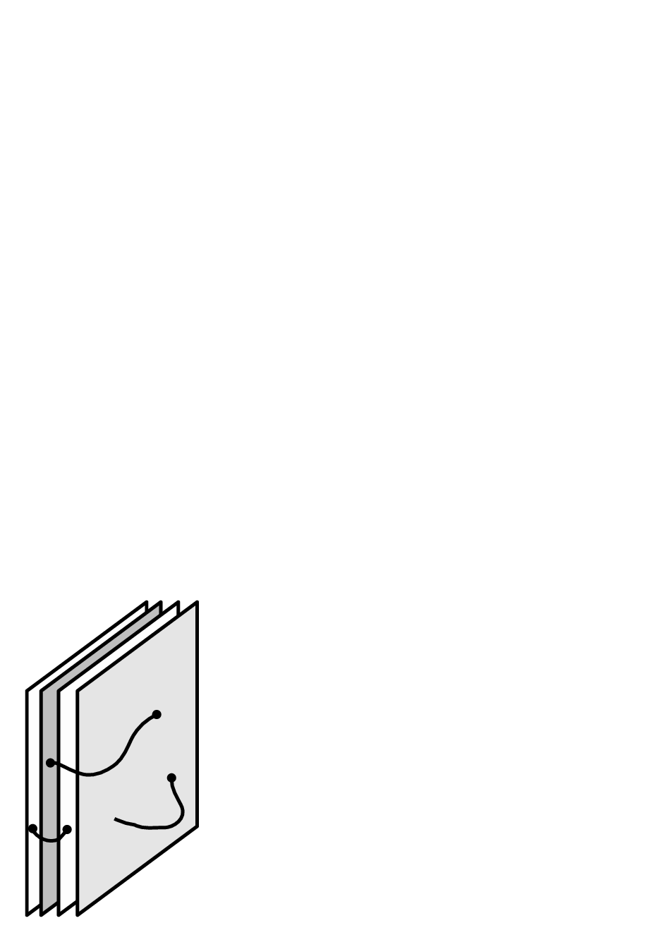
Refer to caption
Figure 10: A stack of NN D-branes, intended to be coincident as well as parallel, but shown separated for clarity. Open strings may begin and end on any two (or the same) branes, without penalty in energy. The effect is that worldvolume fields Xμ​(ξa)X^{\mu}(\xi^{a}) are promoted to N×NN\times N matrices, leading to a non-abelian supersymmetric Yang-Mills theory.

Open strings are free to begin and end on any of the NN branes, without penalty in energy since the branes are coincident. In the N=1N=1 case, the modes of a string parallel to the brane described a gauge field Aa​(ξa)A^{a}(\xi^{a}). Now this field has a factor of N2N^{2} times the number of components in order to allow for the specification of the string end-points’ branes-of-residence. Thus Aa​(ξa)A^{a}(\xi^{a}) is promoted to an N×NN\times N unitary matrix, and similarly for the scalars describing the transverse position of the stack. The full generalization of the action (58) to this case is known [23], but rather than indicating it explicitly here, we give the α′→0\alpha^{\prime}\rightarrow 0 limit of it for the D3-brane, i.e. the generalization of (68)

SN​D​3≃−14​π​gsTr∫d4x(12(Fμ​ν)2+(DμΦI)2−12[ΦI,ΦJ]2+fermions)+…S_{ND3}\simeq-\frac{1}{4\pi g_{s}}\mathop{\mathrm{Tr}}\int d^{4}x\left(\frac{1}{2}(F_{\mu\nu})^{2}+(D_{\mu}\Phi^{I})^{2}-\frac{1}{2}[\Phi^{I},\Phi^{J}]^{2}+\text{fermions}\right)+\ldots (69)

where the trace is over the U⁡(N)U(N) matrix indices, we have changed the worldvolume coordinates to xμx_{\mu}, and the leading constant proportional to volume has been dropped. Here Fμ​ν=∂μAν−∂νAμ−i⁡[Aμ,Aν]F_{\mu\nu}=\partial_{\mu}A_{\nu}-\partial_{\nu}A_{\mu}-i[A_{\mu},A_{\nu}] and Dμ​ΦI=∂μΦI−i⁡[Aμ,ΦI]D_{\mu}\Phi^{I}=\partial_{\mu}\Phi^{I}-i[A_{\mu},\Phi^{I}]. We have indicated “+ fermions” to remind the reader that even equation (58) is only the bosonic portion of the action. All of these objects are supersymmetric and so fermions must be added in the appropriate manner. The action (69) is 𝒩=4{\cal N}=4 supersymmetric Yang-Mills theory in four space-time dimensions. It is a non-abelian U⁡(N)U(N) gauge theory, as we encountered in section 0.3, see equation (5). Comparing the forms of the action, we arrive at the second fundamental relation of the AdS/CFT correspondence

4​π​gs=gY​M2\boxed{4\pi g_{s}=g_{YM}^{2}} (70)

i.e. the Yang-Mills coupling constant is related to the square-root of the closed string coupling.

0.5.2 Absorption cross-sections

We have seen that a stack of NN D3-branes, seen from the low-energy supergravity limit, i.e. away from the branes (see figure 9), looks like a curved spacetime (61) with a five-form field strength turned on. We have also seen that the low-energy limit of the theory on the stack of D-branes is 𝒩=4{\cal N}=4 supersymmetric Yang-Mills with gauge group U⁡(N)U(N). One of the indications that these two pictures might be equivalent came from the consideration of the absorption of closed string modes by either the geometry (61) or by the stack of D-branes [9, 10, 11]. The geometry may be envisioned as having a central throat from which it is difficult for particles to escape, see figure 11.

Refer to caption
Figure 11: The ratio of proper radial distance to coordinate radial distance d​rP/d​r=(1+R4/r4)1/4dr_{P}/dr=(1+R^{4}/r^{4})^{1/4} is plotted on the vertical axis for the extremal 3-brane geometry (61). The angular variable may be thought of as representing the five-sphere. The worldvolume coordinates xix_{i} are suppressed. Here RR is set to one and d​rP/d​rdr_{P}/dr is multiplied by −1-1 for visual effect.

We begin by considering the absorption of the fluctuations of the dilaton Φ\Phi, which we will call ϕ\phi. The equation of motion for this field can be obtained from (51), using the solution (61), (62). It turns out that it is simply □​ϕ=0\Box\phi=0, where the D’Alembertian □\Box is defined by the metric (61). We take the following form for ϕ\phi

ϕ⁡(X)=R⁡(r)​Θ​(Ω5)​e−i​ω​t\phi(X)=R(r)\Theta(\Omega_{5})e^{-i\omega t} (71)

where XX indicates the full 10-dimensional coordinates, rr is the radial coordinate from (61) and Ω5\Omega_{5} is shorthand for the coordinates on the five-sphere. The energy of the fluctuation is given1212 12 As is customary, the units chosen in this thesis are such that ℏ=c=1\hbar=c=1. by ω\omega. Notice that we have suppressed dependence on the brane coordinates xix_{i}; we will not be interested in these fluctuations as they will not contribute to the absorption cross-section. It is straightforward to calculate the D’Alembertian, which then gives the following equation of motion

□ϕ=[−(1+R4r4)∂t2+∂r2+5r∂r+r2DΩ52]ϕ(X)=0\Box\phi=\left[-\left(1+\frac{R^{4}}{r^{4}}\right)\partial_{t}^{2}+\partial_{r}^{2}+\frac{5}{r}\partial_{r}+r^{2}D_{\Omega_{5}}^{2}\right]\phi(X)=0 (72)

where DΩ52D_{\Omega_{5}}^{2} indicates the Laplacian on the five-sphere. We will consider only the s-wave or DΩ52​Θ=0D_{\Omega_{5}}^{2}\Theta=0 modes, and hence calculate the s-wave absorption cross-section. The resulting radial equation is

[ω2(1+R4r4)+r−5∂r(r5∂r)]R(r)=0.\left[\omega^{2}\left(1+\frac{R^{4}}{r^{4}}\right)+r^{-5}\partial_{r}(r^{5}\partial_{r})\right]R(r)=0. (73)

It is simpler to solve this equation after the following change of variables r=R​e−zr=Re^{-z}, R⁡(r)=e2​z​ψR(r)=e^{2z}\psi, then

[∂z2+2ω2R2cosh2z]ψ(z)=0\left[\partial_{z}^{2}+2\omega^{2}R^{2}\cosh 2z\right]\psi(z)=0 (74)

and our problem reduces to a Schrödinger equation with potential −2​ω2​R2​cosh⁡2​z-2\omega^{2}R^{2}\cosh 2z. This is a barrier problem where the incoming wave (from z=−∞z=-\infty) has zero “energy” and the top of the potential is also at zero energy. Thus ψ\psi is on the border between tunnelling or conventionally transmitting from z=−∞z=-\infty to z=∞z=\infty, i.e. from asymptotic flat space at r=∞r=\infty to the center of the throat. The equation may be solved easily in the z→∞z\rightarrow\infty and in the z→−∞z\rightarrow-\infty limits, the solutions are as follows

ψ−∞​(z)≃a​J2​(ω​R​e−z),ψ∞​(z)≃i​H2(1)​(ω​R​ez)\psi_{-\infty}(z)\simeq aJ_{2}(\omega Re^{-z}),\qquad\psi_{\infty}(z)\simeq iH^{(1)}_{2}(\omega Re^{z}) (75)

where Hm(1)H^{(1)}_{m} is the mthm^{\text{th}} Hankel function of the first kind, and J2J_{2} is the second Bessel function. In the region ln⁡ω​R≪z≪−ln⁡ω​R\ln\omega R\ll z\ll-\ln\omega R, i.e. for low energies ω\omega, the two solutions are simultaneously valid, see figure 12. This allows for the determination of the in-going “amplitude” aa, by matching the two solutions in their overlapping region.

Refer to caption
Figure 12: The solutions (75) are plotted for ω​R=0.01\omega R=0.01, where the solid line is ψ−∞​(z)\psi_{-\infty}(z) and the dot-dash the real part of ψ∞​(z)\psi_{\infty}(z) (the imaginary part is negligible). It is seen that they overlap in the region ln⁡ω​R≪z≪−ln⁡ω​R\ln\omega R\ll z\ll-\ln\omega R.

Investigating the asymptotics for z=0z=0 and ω​R≪1\omega R\ll 1, we find

J2​(ω​R​e−z)≃(ω​R)28,i​H2(1)​(ω​R​ez)≃4π​(ω​R)2J_{2}(\omega Re^{-z})\simeq\frac{(\omega R)^{2}}{8},\qquad iH^{(1)}_{2}(\omega Re^{z})\simeq\frac{4}{\pi(\omega R)^{2}} (76)

and so

a=32π​(ω​R)−4.a=\frac{32}{\pi}(\omega R)^{-4}. (77)

The opposite asymptotics give

a​J2​(ω​R​e−z)≃−2π​ω​R​e−z​a2​(ei⁡(ω​R​e−z−π/4)+e−i⁡(ω​R​e−z−π/4)),z→−∞i​H2(1)​(ω​R​ez)≃−i​2π​ω​R​ez​ei⁡(ω​R​ez−π/4),z→∞\begin{split}&aJ_{2}(\omega Re^{-z})\simeq-\sqrt{\frac{2}{\pi\omega Re^{-z}}}\frac{a}{2}\left(e^{i(\omega Re^{-z}-\pi/4)}+e^{-i(\omega Re^{-z}-\pi/4)}\right),\qquad z\rightarrow-\infty\\ &iH^{(1)}_{2}(\omega Re^{z})\simeq-i\sqrt{\frac{2}{\pi\omega Re^{z}}}e^{i(\omega Re^{z}-\pi/4)},\qquad z\rightarrow\infty\end{split} (78)

from which we can read-off the incident, reflection, and transmission coefficients. The absorption probability is the squared norm of the ratio of the transmission coefficient to the incident coefficient, or

𝒫=|1a/2|2=π216​(ω​R)8{\cal P}=\left|\frac{1}{a/2}\right|^{2}=\frac{\pi^{2}}{16}(\omega R)^{8} (79)

The task of translating this into a cross-section is rather involved in the general case [26], the result is the following prescription

σ=(2​π)nωn​Ωn​𝒫=π48​ω3​R8\sigma=\frac{(2\pi)^{n}}{\omega^{n}\Omega_{n}}{\cal P}=\frac{\pi^{4}}{8}\omega^{3}R^{8} (80)

where nn is the dimension of the sphere in the geometry, in our case n=5n=5, while Ωn=2​π(n+1)/2/Γ⁡((n+1)/2)\Omega_{n}=2\pi^{(n+1)/2}/\Gamma((n+1)/2) is the volume of the n-sphere. We have therefore found the absorption cross-section for the dilaton s-waves in the extremal 3-brane geometry.

How do we envision this process from the point of view of the stack of D3-branes? Although we made no mention of it, the action (58) clearly contains a coupling to the dilaton, i.e. the eΦe^{\Phi} factor. We may therefore ask the question, what is the total cross-section for dilaton absorption by a stack of NN D3-branes? In order to answer this question we should begin by analyzing the low-energy limit of our D3-branes and the subsequent dilaton coupling. This is most easily accomplished by placing the action (51) into canonical form by rescaling the metric

Gμ​ν→G~μ​ν=e12​(Φ0−Φ)​Gμ​νG_{\mu\nu}\rightarrow\widetilde{G}_{\mu\nu}=e^{\frac{1}{2}(\Phi_{0}-\Phi)}G_{\mu\nu} (81)

where the dilaton has been shifted by a constant Φ0\Phi_{0}. We will be interested only in the action for the canonically normalized dilaton Φ~=Φ−Φ0\widetilde{\Phi}=\Phi-\Phi_{0}. Applying the rescaling to (51), we have1313 13 Note that R~=eΦ~/2​[R−92​∇2Φ~+92​∂μΦ~​∂μΦ~]\widetilde{R}=e^{\widetilde{\Phi}/2}\left[R-\frac{9}{2}\nabla^{2}\widetilde{\Phi}+\frac{9}{2}\partial_{\mu}\widetilde{\Phi}\partial^{\mu}\widetilde{\Phi}\right], see for example Appendix E of [27].

S10=12​(κ10​eΦ0)2​∫d10​x​−G~​(R~−12​∂μΦ~​∂μΦ~+…).S_{10}=\frac{1}{2(\kappa_{10}e^{\Phi_{0}})^{2}}\int d^{10}x\sqrt{-\widetilde{G}}\left(\widetilde{R}-\frac{1}{2}\partial_{\mu}\widetilde{\Phi}\partial^{\mu}\widetilde{\Phi}+\ldots\right). (82)

This frame is referred to as the Einstein frame, while the pre-scaled version is dubbed the string frame. Notice that the gravitational coupling is determined by the constant dilaton shift, κ~10=κ10​eΦ0=κ10​gs\widetilde{\kappa}_{10}=\kappa_{10}e^{\Phi_{0}}=\kappa_{10}g_{s}. Shifting to the Einstein frame in our D-brane action (58), we see that only the Ga​bG_{ab} term is affected. The result for the low-energy action of our stack of D3-branes is

S4=−12​gY​M2Tr∫d4x(e−Φ~(Fα​β)2+…)S_{4}=-\frac{1}{2g^{2}_{YM}}\mathop{\mathrm{Tr}}\int d^{4}x\left(e^{-\widetilde{\Phi}}(F_{\alpha\beta})^{2}+\ldots\right) (83)

where the “…\ldots’’ refers to terms not coupled to the dilaton and fermion terms1414 14 The in-coming dilaton s-wave cannot be converted into a pair of fermions on the brane because the coupling, involving the kinetic term ψ¯​∂̸ψ\bar{\psi}\displaystyle{\not}\partial\psi, gives an odd power of the momentum.. Also, we have omitted couplings to the dilaton involving the transverse scalars on the D-brane; these correspond to higher-than-s-wave dilaton couplings. We now take G~μ​ν=ημ​ν\widetilde{G}_{\mu\nu}=\eta_{\mu\nu} since we take the D3-branes to be sitting in flat ten-dimensional space. Further, we put the dilaton action (82) into standard canonical form by defining ϕ=Φ~/2​κ~10\phi=\widetilde{\Phi}/\sqrt{2}{\widetilde{\kappa}_{10}}; we do the same for the coupling in (83) by rescaling AαA_{\alpha} by gY​Mg_{YM}. We then obtain

S10+S4=−12∫d10x∂μϕ∂μϕ−∫d4ξ(14(Fα​βa)2+κ~102ϕ∂αAβa∂αAa​β)S_{10}+S_{4}=-\frac{1}{2}\int d^{10}x\,\partial_{\mu}\phi\,\partial^{\mu}\phi-\int d^{4}\xi\left(\frac{1}{4}(F_{\alpha\beta}^{a})^{2}+\frac{\widetilde{\kappa}_{10}}{\sqrt{2}}\,\phi\,\partial_{\alpha}A^{a}_{\beta}\,\partial^{\alpha}A^{a\beta}\right) (84)

where we have used the fact that the generators TaT^{a} of U⁡(N)U(N) are normalized by Tr(Ta​Tb)=12​δa​b\mathop{\mathrm{Tr}}(T^{a}T^{b})=\tiny{\frac{1}{2}}\delta^{ab} where the index aa runs from 1 to N2N^{2}. The problem of calculating the cross-section is now straightforward, and can be found in any textbook on quantum field theory, see for example [28], pg. 107. The field AαaA^{a}_{\alpha} will have two physical polarizations for each aa. At leading order in λ=gY​M2​N\lambda=g_{YM}^{2}N, each will couple to an in-coming dilaton ϕ\phi (solid line below) via the following Feynman diagram

[Uncaptioned image]

where the piα{p_{i}}^{\alpha} are the four-momenta of the final state photons (wiggly lines above). The cross-section is then given by

σ=12​12​ω​∫d3​p1(2​π)3​12​E1​∫d3​p2(2​π)3​12​E2​(2​π)4​δ​(E1+E2−ω)​δ3​(p→1+p→2)​|ℳ|2=κ~102​ω364​π\sigma=\frac{1}{2}\frac{1}{2\omega}\int\frac{d^{3}p_{1}}{(2\pi)^{3}}\frac{1}{2E_{1}}\int\frac{d^{3}p_{2}}{(2\pi)^{3}}\frac{1}{2E_{2}}(2\pi)^{4}\delta(E_{1}+E_{2}-\omega)\delta^{3}(\vec{p}_{1}+\vec{p}_{2})\,|{\cal M}|^{2}=\frac{\widetilde{\kappa}_{10}^{2}\omega^{3}}{64\pi} (85)

where ω\omega is the energy of the in-coming dilaton and the leading factor of 1/21/2 accounts for the fact that the final-state photons are identical. Since we have 2​N22N^{2} species of photons, where the 22 counts the number of physically distinct polarizations, we have

σt​o​t=N2​κ~102​ω332​π.\sigma_{tot}=\frac{N^{2}\widetilde{\kappa}_{10}^{2}\omega^{3}}{32\pi}. (86)

Using the fact that κ~102=(2​π)7​gs2​α′4/2\widetilde{\kappa}_{10}^{2}=(2\pi)^{7}g_{s}^{2}\alpha^{\prime 4}/2, and (65) we see that this is identical to (80). Therefore, for the dilaton s-wave, the stack of D3-branes in flat 10-dimensional space absorbs exactly the same as the throat of the geometry (61). In fact the agreement is suspicious. The supergravity result (80) is valid in the supergravity approximation, i.e. when R4/α′2=gY​M2​N≫1R^{4}/\alpha^{\prime 2}=g_{YM}^{2}N\gg 1, but we performed our D-brane calculation only to leading order in λ=gY​M2​N\lambda=g_{YM}^{2}N, i.e. in the R4/α′2≪1R^{4}/\alpha^{\prime 2}\ll 1 limit. In fact the higher order corrections to (86) vanish as a result of a non-renormalization theorem [11]. The cross-sections for other closed string modes, namely fermions and gravitons, were found to agree similarly in [10].

This result was an indication that there was a duality emerging between strongly coupled super-Yang-Mills and IIB strings on a weakly curved background. In fact there was already an indication from a study of entropy [12], that a correspondence may be at play. It was found that the entropy of the weakly coupled super-Yang-Mills theory at small temperature agreed with that of the corresponding near-extremal black hole entropy, up to a factor of 4/34/3. This near match for quantities at opposite ends of the coupling spectrum was notable. Maldacena [13] eventually codified these observations into a conjecture which has largely shaped string theory research in the interim.

0.5.3 The Maldacena conjecture

The central theme in the Maldacena conjecture is a decoupling limit. Specifically, Maldacena considered taking R,α′→0R,\alpha^{\prime}\rightarrow 0 while keeping R4/α′2=λ=4​π​gs​NR^{4}/\alpha^{\prime 2}=\lambda=4\pi g_{s}N fixed. This limit sends the cross-section (86) to zero; the strings in the throat of (61) (on the stack of D-branes) are decoupled from those in the asymptotic region (away from the stack of D-branes). This results in two pictures, each containing two decoupled theories. In the throat-geometry picture we have closed, type IIB strings propagating in the r≪Rr\ll R region of (61)

d​s2=r2R2​(−d​t2+d​xi2)+R2r2​(d​r2+r2​d​Ω52)ds^{2}=\frac{r^{2}}{R^{2}}\left(-dt^{2}+dx_{i}^{2}\right)+\frac{R^{2}}{r^{2}}\left(dr^{2}+r^{2}d\Omega_{5}^{2}\right) (87)

which are decoupled from closed IIB strings propagating out at r≫Rr\gg R, which is just 10-dimensional flat space. In the D-brane picture we have 𝒩=4{\cal N}=4 super-Yang-Mills in four spacetime dimensions with gauge group U⁡(N)U(N) on the stack of D-branes, while decoupled closed, type IIB strings propagate in the bulk spacetime which is 10-dimensional flat space. The two pictures share a decoupled theory: closed type IIB strings in 10-dimensional flat space. The Maldacena conjecture [13] posits that the other two decoupled theories are also equivalent, that is

𝒩=4{\cal N}=4 super-Yang-Mills in four spacetime dimensions with gauge group U⁡(N)U(N) is dual to type IIB string theory on the background A​d​S5×S5AdS_{5}\times S^{5}

where we have identified (87) as the metric of five dimensional anti de-Sitter space times a five-sphere. We should also not forget that this background includes the form-field strength (62). What does this duality imply about the two theories? The super-Yang-Mills has two parameters; NN the rank of the gauge group, and λ=gY​M2​N\lambda=g^{2}_{YM}N the ’t Hooft coupling. The decoupling limit keeps λ\lambda fixed. This means that when NN is varied, gY​M2=4​π​gsg^{2}_{YM}=4\pi g_{s} varies inversely. Thus the closed string coupling varies inversely with NN, so that when NN is large the closed string dynamics are captured by their tree-level or classical limit, see figure 13. The ’t Hooft coupling itself may also be varied. From (65) we see that λ\lambda measures the ratio of the AdS (and five-sphere) curvature to the string length (α′\sqrt{\alpha^{\prime}}). Thus when λ\lambda is large, i.e. the gauge theory is strongly coupled, the “stringiness” of the closed strings is suppressed and they are well approximated by their low-energy point-particle limit: type IIB supergravity.
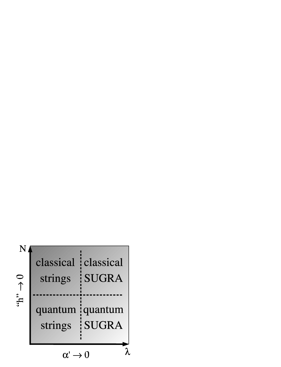
Refer to caption
Figure 13: The parametric limits of the AdS/CFT correspondence. The rank of the super-Yang-Mills gauge group NN controls quantum corrections in the closed string theory; these correspond to non-planar gauge theory processes. The ’t Hooft coupling controls the ratio of the closed string background curvature to the string length; large ’t Hooft coupling corresponds to point-particle supergravity (“SUGRA”). Here “h” refers to the effective Planck’s constant - i.e. the parameter controlling “quantumness”.

The beauty of this correspondence is that (at least for large NN) it is precisely where the analytical techniques fail in the gauge theory, i.e. at large λ\lambda, that the dual string theory simplifies to classical supergravity on a weakly curved background. We have analytical control over the dual theory in this regime, and so we have finally realized a string description of a strongly coupled gauge theory that will allow analytical calculations.

0.5.4 Preliminary evidence for AdS/CFT: symmetries

We have presented a conjecture in section 0.5.3 with no evidence or proof. What is the main motivation, above and beyond the cross-section calculations of section 0.5.2, for suggesting this duality? The answer is that the two theories share the same symmetry groups. 𝒩=4{\cal N}=4, d=4d=4 supersymmetric Yang-Mills theory is believed to be a conformal field theory or CFT. The meaning of this is that the full interacting, quantum mechanical theory is invariant under conformal transformations. These are angle-preserving transformations which include global rescalings

xμ→Λ​xμx^{\mu}\rightarrow\Lambda x^{\mu} (88)

and the so-called special conformal transformations

xμ→xμ+aμ​x21+2​aμ​xμ+a2​x2x^{\mu}\rightarrow\frac{x^{\mu}+a^{\mu}x^{2}}{1+2a_{\mu}x^{\mu}+a^{2}x^{2}} (89)

where aμa^{\mu} is some real d-vector. A natural consequence of invariance under (88) is that the β\beta-function for the coupling gY​Mg_{YM} is identically zero. This means that the coupling in a CFT does not run at all - it is a free parameter in the theory. This is important for the duality of AdS/CFT since we would like to be able to vary the ’t Hooft coupling λ\lambda freely (see figure 13). The conformal group extends the symmetry of flat space (31), i.e. the Poincaré group, via the inclusion of the generators of (88) DD, and those of (89) KμK_{\mu}. The extra algebraic relations are

[D,Pμ]=−i​Pμ,[Pμ,Kν]=2iMμ​ν−2iημ​νD,[D,Kμ]=iKμ,[Mμ​ν,D]=0,[Mμ​ν,Kρ]=−i⁡(ημ​ρ​Kν−ην​ρ​Kμ).\begin{split}[D,P_{\mu}]=-iP_{\mu},\qquad[P_{\mu},K_{\nu}]&=2iM_{\mu\nu}-2i\eta_{\mu\nu}D,\qquad[D,K_{\mu}]=iK_{\mu},\\ [M_{\mu\nu},D]=0,\qquad&[M_{\mu\nu},K_{\rho}]=-i(\eta_{\mu\rho}K_{\nu}-\eta_{\nu\rho}K_{\mu}).\end{split} (90)

In fact the conformal group is isomorphic to S​O​(2,d)SO(2,d). This can be seen via the following assignments

Jμ​ν=Mμ​ν,Jμ​d=12​(Kμ−Pμ),Jμ⁡(d+1)=12​(Kμ+Pμ),J(d+1)​d=D,J_{\mu\nu}=M_{\mu\nu},\qquad J_{\mu d}=\frac{1}{2}(K_{\mu}-P_{\mu}),\qquad J_{\mu\,(d+1)}=\frac{1}{2}(K_{\mu}+P_{\mu}),\qquad J_{(d+1)\,d}=D, (91)

for which [JM​N,JI​J]=i​ηN​I​JM​J−i​ηM​I​JN​J−i​ηN​J​JM​I+i​ηM​J​JN​I[J_{MN},J_{IJ}]=i\eta_{NI}J_{MJ}-i\eta_{MI}J_{NJ}-i\eta_{NJ}J_{MI}+i\eta_{MJ}J_{NI} simply gives the conformal group relations, where I,J,M,N=0,…,d+1I,J,M,N=0,\ldots,d+1 with signature (−,+,…,+,−)(-,+,\ldots,+,-). 𝒩=4{\cal N}=4 super-Yang-Mills (69) contains another important symmetry group, called R-symmetry. This symmetry rotates the six scalar fields ΦI\Phi^{I} into one another; therefore this group is S​O​(6)SO(6). On the level of bosonic symmetries, this is it. Thus the bosonic symmetries of 𝒩=4{\cal N}=4 super-Yang-Mills is S​O​(2,4)×S​O​(6)SO(2,4)\times SO(6).

Anti de-Sitter space may be defined as the embedding of a hyperboloid in a two-time signature space

ds2=−dx02−dxd+12+(dxi)2,i=1,…,d.ds^{2}=-dx_{0}^{2}-dx_{d+1}^{2}+(dx_{i})^{2},\qquad i=1,\ldots,d. (92)

The hyperboloid is embedded as

x02+xd+12−(xi)2=R2x_{0}^{2}+x_{d+1}^{2}-(x_{i})^{2}=R^{2} (93)

which is manifestly S​O​(2,d)SO(2,d) invariant. It is then plain to see that the isometry group of the space A​d​S5×S5AdS_{5}\times S^{5} is S​O​(2,4)×S​O​(6)SO(2,4)\times SO(6). We have therefore an exact matching of the bosonic symmetries between 𝒩=4{\cal N}=4 super-Yang-Mills and fields on A​d​S5×S5AdS_{5}\times S^{5}. In fact it can be shown that the full supergroup of type IIB strings on A​d​S5×S5AdS_{5}\times S^{5} and 𝒩=4{\cal N}=4 super-Yang-Mills is S​U​(2,2|4)SU(2,2|4), of which S​O​(2,4)×S​O​(6)SO(2,4)\times SO(6) is the bosonic subgroup.

It will be useful to explore anti de-Sitter space more thoroughly. The hyperboloid (93) may be coordinatized using the following relations

x0=R​cosh⁡ρ​cos⁡τ,xd+1=R​cosh⁡ρ​sin⁡τ,xi=R​sinh⁡ρ​Ωi,(Ωi)2=1x_{0}=R\cosh\rho\cos\tau,\qquad x_{d+1}=R\cosh\rho\sin\tau,\qquad x_{i}=R\sinh\rho\,\Omega_{i},\qquad(\Omega_{i})^{2}=1 (94)

where Ωi\Omega_{i} are an embedding of the (d−1)(d-1)-sphere. This leads to so-called global AdS

d​s2=R2​(−cosh2⁡ρ​d​τ2+d​ρ2+sinh2⁡ρ​d​Ωd−12)ds^{2}=R^{2}(-\cosh^{2}\rho\,d\tau^{2}+d\rho^{2}+\sinh^{2}\rho\,d\Omega_{d-1}^{2}) (95)

where the coordinate τ\tau is unwrapped from its fundamental domain [−π,π][-\pi,\pi] to [−∞,∞][-\infty,\infty] in order to avoid closed timelike curves, while ρ∈[0,∞]\rho\in[0,\infty]. Another important coordinatization is

x0=12​r(1+r2​(R2+z→2−t2)),xd=12​r​(1−r2​(R2−z→2+t2)),xa=Rrza,xd+1=Rrt,a=1,…,d−1\begin{split}x_{0}=\frac{1}{2r}&\left(1+r^{2}(R^{2}+\vec{z}^{2}-t^{2})\right),\qquad x_{d}=\frac{1}{2r}\left(1-r^{2}(R^{2}-\vec{z}^{2}+t^{2})\right),\\ &~~~x_{a}=Rrz_{a},\qquad x_{d+1}=Rrt,\qquad a=1,\ldots,d-1\end{split} (96)

where r≥0r\geq 0 and tt and z→\vec{z} are unconstrained. This gives the Poincaré patch

d​s2=r2R2​(−d​t2+d​z→2)+R2r2​d​r2ds^{2}=\frac{r^{2}}{R^{2}}\left(-dt^{2}+d\vec{z}^{2}\right)+\frac{R^{2}}{r^{2}}dr^{2} (97)

which we saw in (87). The global coordinates (95) cover the entire hyperboloid (93) once, the Poincaré patch, as we will see, covers only half of it. The relationship between the global and Poincaré coordinates systems is most easily seen when d=2d=2, i.e. for A​d​S3AdS_{3}. In this case the Ωi\Omega_{i} parametrizes a circle whose parameter we will take as ϕ\phi, and we have

r=1R​(cosh⁡ρ​cos⁡τ−sinh⁡ρ​cos⁡ϕ),t=R​cosh⁡ρ​sin⁡τcosh⁡ρ​cos⁡τ−sinh⁡ρ​cos⁡ϕ,z=R​sinh⁡ρ​sin⁡ϕcosh⁡ρ​cos⁡τ−sinh⁡ρ​cos⁡ϕ.\begin{split}r=\frac{1}{R}\left(\cosh\rho\cos\tau-\sinh\rho\cos\phi\right),~~~~~~~~~~~~~~\\ \qquad t=\frac{R\cosh\rho\sin\tau}{\cosh\rho\cos\tau-\sinh\rho\cos\phi},\qquad z=\frac{R\sinh\rho\sin\phi}{\cosh\rho\cos\tau-\sinh\rho\cos\phi}.\end{split} (98)

Since r≥0r\geq 0, we must have cos⁡τ≥tanh⁡ρ​cos⁡ϕ\cos\tau\geq\tanh\rho\cos\phi. The boundary of the patch is therefore given by the following curves (see figure 14, right panel, where ρ\rho is set to infinity)

τ=±arccos⁡(tanh⁡ρ​cos⁡ϕ).\tau=\pm\arccos\left(\tanh\rho\cos\phi\right). (99)

One may verify that the area (in the τ\tau-ϕ\phi plane) of the patch is therefore given by

4​∫0πd​ϕ​arccos⁡(tanh⁡ρ​cos⁡ϕ)=2​π24\int_{0}^{\pi}d\phi\arccos\left(\tanh\rho\cos\phi\right)=2\pi^{2} (100)

independently of ρ\rho. This is one half of the total area, 4​π24\pi^{2} (since τ\tau and ϕ\phi are ∈[0,2​π]\in[0,2\pi]).

Anti de-Sitter space also has a time-like boundary which is most easily seen through the change of coordinates tan⁡θ=sinh⁡ρ\tan\theta=\sinh\rho, where θ∈[0,π/2]\theta\in[0,\pi/2]. The global A​d​SAdS metric (95) then takes the following form

d​s2=R2cos2⁡θ​(−d​τ2+d​θ2+sin2⁡θ​d​Ωi2).ds^{2}=\frac{R^{2}}{\cos^{2}\theta}(-d\tau^{2}+d\theta^{2}+\sin^{2}\theta d\Omega_{i}^{2}). (101)

The boundary is found at spatial infinity (θ=π/2\theta=\pi/2 or ρ=∞\rho=\infty) and is of the form ℝ×Sd−1\mathbb{R}\times S^{d-1}. A Penrose diagram of the space is shown in figure (14).

Refer to caption
Refer to caption
Figure 14: A Penrose diagram of anti de-Sitter space (101) is shown on the left. The diamonds are the paths of light-rays beginning at θ=0\theta=0, τ=−π\tau=-\pi and reflecting off the boundary at θ=π/2\theta=\pi/2. A signal from the boundary (which is at spatial infinity) may propagate into the spacetime in finite coordinate time. Note that the diagram should be understood to be a fundamental domain which is periodically continued to τ=[−∞,∞]\tau=[-\infty,\infty] The angle ϕ\phi is understood as the azimuthal angle in the Ωi\Omega_{i} portion of the metric. On the right the boundary (r=∞r=\infty) of the Poincaré patch (97) is displayed for d=2d=2. The boundary of global A​d​S3AdS_{3} may be envisioned as a cylinder with a coordinate τ\tau running along the length of the cylinder and the angle ϕ\phi going around it. The Poincaré patch fits into half a fundamental domain, bounded by null surfaces at spatial infinity (z=±∞z=\pm\infty) forming a diamond shape which wraps around the cylinder. The horizontal curves are lines of constant zz, while the vertical curves are lines of constant tt.

The boundary is time-like and it takes a finite amount of coordinate time for a signal to propagate from the boundary at spatial infinity to any point in the space. This implies that information may be gained from or lost to the boundary, and in this respect anti de-Sitter space is very similar to Minkowski space in a box. This will be important for us in the next section. The boundary in the Poincaré patch is at r=∞r=\infty and is given by d​s2=r2​(−d​t2+d​z→2)/R2ds^{2}=r^{2}(-dt^{2}+d\vec{z}^{2})/R^{2}; i.e. it is a conformal rescaling of flat d-dimensional space. In this sense the Poincaré coordinates “lose the point at infinity” required to restore the ℝ×Sd−1\mathbb{R}\times S^{d-1} topology of the boundary.

0.5.5 The field-operator dictionary and the GKP-W relation

The AdS/CFT correspondence alleges an equivalence between a conformal field theory and a string theory on A​d​S5×S5AdS_{5}\times S^{5}, but how is the equivalence seen? In order to specify what is equivalent to what, a dictionary is required which translates a problem posed in one setting into the language of the other, and vice-versa. Such a dictionary is given by the GKP-W relation [29, 30], named for Gubser, Klebanov, Polyakov, and Witten. The first question we should ask is what are the meaningful (physical) quantities in each of the theories that are eligible for comparison. A conformal field theory or CFT has no scale, it is therefore meaningless to discuss asymptotically free wave-packets, and this precludes an S-matrix and the concept of particles with definite mass. An important class of invariants that a CFT does possess is the scaling dimensions of operators. These must relate to some other invariant in the gravity (string) theory. Supergravity in A​d​S5×S5AdS_{5}\times S^{5} does have a scale and asymptotic mass eigenstates. We mentioned in section 0.5.4 that in some respects A​d​SAdS space is similar to Minkowski space in a box. In fact, a unique solution to the Laplace equation for a (for example scalar) field ϕ⁡(r,z→,t)\phi(r;\vec{z},t) on A​d​SAdS requires the specification of boundary data ϕ0​(z→,t)=ϕ⁡(∞,z→,t)\phi_{0}(\vec{z},t)=\phi(\infty;\vec{z},t). Keeping these facts in mind, the absorption cross-section calculations of section 0.5.2 hint at what the relation between the CFT and the supergravity should be. Recall that the coupling of the dilaton to the D-brane worldvolume theory (at low energy) was (83) ∼Tr∫⁡d4​x​ϕ0​F2\sim\mathop{\mathrm{Tr}}\int d^{4}x\phi_{0}F^{2}. That is, the bulk closed string mode described by the field ϕ\phi, interacts with the worldvolume theory via a local (i.e. proportional to the value of ϕ\phi on the space where the worldvolume theory lives, that is, ϕ0\phi_{0}) coupling to an operator of the CFT. In the throat of the geometry, ϕ\phi represents a minimization of the supergravity action on A​d​S5AdS_{5}, subject to the boundary condition ϕ0\phi_{0}. This minimized action therefore appears equivalent to the addition of the operator 𝒪=TrF2{\cal O}=\mathop{\mathrm{Tr}}F^{2} to the worldvolume theory’s action, SW​V→SW​V+∫d4​x​ϕ0​𝒪S_{WV}\rightarrow S_{WV}+\int d^{4}x\phi_{0}{\cal O}. To be more precise, the GKP-W relation is

⟨exp⁡(∫d4​x​ϕ0​𝒪)⟩C​F​T=exp⁡(−SSUGRA​(ϕ)).\boxed{\left<\exp\left(\int d^{4}x\,\phi_{0}\,{\cal O}\right)\right>_{CFT}=\exp\left(-S_{\text{SUGRA}}(\phi)\right)}. (102)

It may seem confusing that ϕ0\phi_{0} is at once the value of the field ϕ\phi on the stack of D-branes and the value on the boundary of A​d​S5AdS_{5}. What must be remembered is that in the decoupling limit (see section 0.5.3), the throat region, which is identified with the position of the D-branes, is blown-up to the entire space A​d​S5×S5AdS_{5}\times S^{5}. In this near horizon geometry, where has the corresponding position of the stack of D-branes gone? The answer is to the boundary of A​d​S5AdS_{5}. Indeed we saw in section 0.5.4 that this boundary is conformally equivalent to four-dimensional flat space. In fact, the S​O​(2,4)SO(2,4) isometry group of A​d​S5AdS_{5} acts upon this boundary as the four-dimensional conformal group. It should be emphasized that it is a mistake to think of the CFT as living on the boundary of A​d​S5AdS_{5} simultaneously with the supergravity in the bulk. They are conjectured as equivalent descriptions of the same physics; we can either work with the full A​d​S5AdS_{5} supergravity or we can throw that away and answer the same questions with the holographic CFT. To see that this is so we can work out a simple example in which it will be revealed that the relation (102) actually implies an equivalence between the scaling dimension of the operator 𝒪{\cal O} and the mass of the associated field ϕ\phi. It is simplest to employ the Poincaré metric (97), in Euclidean signature, and with the coordinate redefinition r→R2/yr\rightarrow R^{2}/y,

d​s2=R2y2​(d​y2+d​xi2)ds^{2}=\frac{R^{2}}{y^{2}}(dy^{2}+dx_{i}^{2}) (103)

where the Euclideanized boundary space at y=0y=0 is now covered by the coordinates xix_{i}. The Green’s function corresponding to a field ϕ⁡(y,xi)\phi(y,x_{i}) specified by boundary data ϕ⁡(0,xi)\phi(0,x_{i}) is most easily obtained from an S​O​(1,d+1)SO(1,d+1) transformed version depending only on yy [30]

K⁡(y)=C​ydK(y)=Cy^{d} (104)

where CC is some constant. This ansätz obeys the equation of motion □​ϕ=0\Box\phi=0 and the boundary condition K⁡(∞)=∞K(\infty)=\infty. Under the S​O​(1,d+1)SO(1,d+1) inversion

y→yy2+xi2,xi→xiy2+xi2y\rightarrow\frac{y}{y^{2}+x_{i}^{2}},\qquad x_{i}\rightarrow\frac{x_{i}}{y^{2}+x_{i}^{2}} (105)

the Green’s function (104) becomes

K⁡(y,xi)=C​yd(y2+xi2)dK(y,x_{i})=C\frac{y^{d}}{(y^{2}+x_{i}^{2})^{d}} (106)

which gives (for properly chosen CC) the behaviour K⁡(0,xi)=δd​(xi)K(0,x_{i})=\delta^{d}(x_{i}) at the boundary point y=0y=0. This is the desired boundary condition for a bulk-to-boundary propagator, as it defines the bulk field ϕ⁡(y,xi)\phi(y,x_{i}) in terms of its boundary value ϕ⁡(0,xi)\phi(0,x_{i}) in the following manner

ϕ⁡(y,xi)=∫dd​x~i​C​yd(y2+(xi−x~i)2)d​ϕ​(0,x~i).\phi(y,x_{i})=\int d^{d}\widetilde{x}_{i}\frac{Cy^{d}}{(y^{2}+(x_{i}-\widetilde{x}_{i})^{2})^{d}}\,\phi(0,\widetilde{x}_{i}). (107)

We should now plug this solution into the RHS of (102). The action for a massless scalar field is

S⁡[ϕ]=12​∫dd​xi​∫d​y​g​∂μϕ​∂μϕS[\phi]=\frac{1}{2}\int d^{d}x_{i}\,\int dy\,\sqrt{g}\,\partial_{\mu}\phi\,\partial^{\mu}\phi (108)

where μ\mu runs over all d+1d+1 coordinates of (103) which is also the metric gμ​νg_{\mu\nu} refers to. Plugging the solution (107) into this action gives only a surface term at y=0y=0, since the main part of the action vanishes by the equation of motion. It is straightforward to show that

S⁡[ϕ⁡(y,xi)]=C​d2​∫dd​xi​∫dd​x~i​ϕ⁡(0,xi)​ϕ​(0,x~i)(xi−x~i)2​d.S[\phi(y,x_{i})]=\frac{Cd}{2}\int d^{d}{x_{i}}\int d^{d}{\widetilde{x}_{i}}\frac{\phi(0,x_{i})\,\phi(0,\widetilde{x}_{i})}{(x_{i}-\widetilde{x}_{i})^{2d}}. (109)

The two-point function of an operator 𝒪⁡(x){\cal O}(x) in the CFT of conformal weight dd has the following behaviour

⟨𝒪⁡(xi)​𝒪​(x~i)⟩=𝒞(xi−x~i)2​d\langle{\cal O}(x_{i})\,{\cal O}(\widetilde{x}_{i})\rangle=\frac{{\cal C}}{(x_{i}-\widetilde{x}_{i})^{2d}} (110)

where 𝒞{\cal C} is a constant. It is immediately seen that for the appropriate choice of the constant CC, the LHS of (102) is exactly (109), where we have taken only the quadratic term in the expansion of the exponentials, i.e. we are comparing two-point functions. This whole story is repeated for the case of a massive field ((□−m2)​ϕ=0(\Box-m^{2})\phi=0) with the replacement1515 15 The number of CFT spacetime dimensions remain dd. The other difference is in the relation of the CFT scalar ϕ0​(xi)\phi_{0}(x_{i}) to the boundary behaviour of the bulk field ϕ⁡(y,xi)\phi(y,x_{i}); the general relationship is limy→0ϕ⁡(y,xi)=yd−Δ​ϕ0​(xi)\lim_{y\rightarrow 0}\phi(y,x_{i})=y^{d-\Delta}\phi_{0}(x_{i}).

d→Δ=12​(d+d2+4​m2).d\rightarrow\Delta=\frac{1}{2}\left(d+\sqrt{d^{2}+4m^{2}}\right). (111)

We therefore have that the dual of the scaling dimension Δ\Delta of an operator 𝒪{\cal O} in the CFT is related to the mass mm of the dual AdS field by (111).

0.5.6 Beyond two-point functions

The AdS/CFT correspondence has passed many tests beyond the two-point function presented in section 0.5.5. We will not give a detailed account of the various successes of the correspondence here, as that would fill several review papers. Three point functions are well understood [32], and are protected by conformal invariance in the CFT. Four point functions do not share this protection, but have been studied extensively (see references [92] through [104]). There are also large bodies of work concerning Wilson loops (see chapter The AdS/CFT Correspondence: Classical, Quantum, and Thermodynamical Aspects), M-theory (see chapter The AdS/CFT Correspondence: Classical, Quantum, and Thermodynamical Aspects), thermodynamics, D-brane states, macroscopic strings, viscosity, black-hole entropy and information loss, and more. Indeed Maldacena’s original paper [13] has been cited over 4500 times at the time of writing, and appears to be increasing roughly linearly with time, see figure 15.

Refer to caption
Figure 15: Citations of Maldacena’s original paper [13] as a function of time, loosely interpreted from the citebase website [105]. The current SPIRES count is more than 4500.

The AdS/CFT correspondence has been the main focus of string theory research for the past decade. Although a proof of the correspondence is still lacking, no test of AdS/CFT has returned a negative result. Much of the work on the correspondence has naturally focused on the classical regime where large-NN super-Yang-Mills at strong coupling is compared with supergravity. True quantum tests, involving 1/N1/N corrections, are less prevalent and less definitive, as we will see in chapter The AdS/CFT Correspondence: Classical, Quantum, and Thermodynamical Aspects. The quantum and stringy limits of AdS/CFT are the most important avenues to study, in order to further the evidence that the correspondence is indeed correct.

0.6 Summary

We began this chapter with the clash of two titans, strongly coupled gauge theory and gravity. String theory, devised to study the former, was retired and then refitted to study the latter. In the end it led to a remarkable observation, that in a certain context, the two titans are reflections of each other, descriptions of the same physics encoded in a different language. Further, the questions that are most difficult to answer in one description are the easiest to answer in the other. The stage is thus set for an exploration of this gauge/string duality. In the following three chapters of this thesis, we will present work concerning the quantum (chapter The AdS/CFT Correspondence: Classical, Quantum, and Thermodynamical Aspects), thermodynamic (chapter The AdS/CFT Correspondence: Classical, Quantum, and Thermodynamical Aspects), and classical (chapter The AdS/CFT Correspondence: Classical, Quantum, and Thermodynamical Aspects) aspects of the AdS/CFT correspondence. This research represents some important steps in the very long journey to fully understanding the breadth and mechanisms of this remarkable duality.

Chapter 0 Light-cone string field theory on the plane-wave

I call the loose snow to fly
from your rooftops, the timorous doves
from your rafters’ sanctum.

— Ruth Taylor The Dragon Papers, Emanations                                            

String theory, despite all its complexity and scope, remains a first-quantized theory. It is fundamentally the quantum dynamics of a single relativistic string. The theory lacks a Lagrangian which would dictate the full interacting theory of a field of strings. From the point particle analogue point of view, we have only quantum mechanics - not quantum field theory. This lack of completeness has not prevented string theorists from considering on-shell string interactions in some detail (c.f. [33, 34, 35, 36]), guided simply by the symmetries inherent in the first quantized theory, and by the manner in which strings interact with background fields. To be more precise, we have some control over interactions in the supergravity limit (as discussed in section 0.4.6), where we know the full point-particle Lagrangian is given by supergravity. On-shell scattering amplitudes for low-lying string modes (i.e. few excitations), with small numbers of loops (<3<3), were calculated very early on. Continuing string interactions off the mass-shell has enjoyed a certain amount of success using Witten’s cubic string field theory [37], see [38] for a recent review. From the point of view of light-cone gauge quantization (see section 0.4.5), the description of the most basic interaction - the three string vertex - is simply a map between the collections of oscillators (45) which completely specify each string, see figure 16.

Refer to caption
Figure 16: In light-cone string field theory the cubic interaction vertex may be considered as a map between the collections of oscillators αn\alpha_{n} and βm\beta_{m} which completely specify each string.

Such a map was developed by Green, Schwarz, and Brink [45, 46] in the early 1980’s, for type II superstrings in a flat target space background. In 2002, Spradlin and Volovich [53, 54] generalized this work to the plane-wave background. In that context, the light-cone string field theory may be used to calculate one-loop shifts to the masses of string states. These are dual to anomalous dimensions of certain operators in 𝒩=4{\cal N}=4 super-Yang-Mills (in a given limit) and may be compared as a check on the AdS/CFT correspondence1616 16 For reviews of the plane-wave string / gauge theory duality see [51] and [52].. This chapter will introduce this program, and present original work by the author which clarified some oblique issues concerning the importance of intermediate string states in the one-loop mass shifts, proved the finiteness of those shifts, and culminated in the best match so far discovered between the gauge and string theory results using a version of the string interaction vertex proposed by Dobashi and Yoneya [57].

0.7 The plane-wave background and the BMN limit of 𝒩=4{\cal N}=4 SYM

In section 0.5 the AdS/CFT correspondence was introduced as a conjectured equivalency between type IIB superstrings on A​d​S5×S5AdS_{5}\times S^{5} and 𝒩=4{\cal N}=4 SYM. An early stumbling block encountered by investigators of the correspondence was solving the string sigma model (curved space analogue of 39) on this background. This remains an obstacle which has yet to be overcome. Without the rudimentary information provided by the free string spectrum on A​d​S5×S5AdS_{5}\times S^{5}, understanding or even testing the AdS/CFT correspondence beyond the supergravity limit is extremely limited. In 2001, a new type IIB background space was found [58] which, like A​d​S5×S5AdS_{5}\times S^{5}, is maximally supersymmetric. This is the so-called plane-wave background and is given by

d​s2=−2​d​x−​d​x+−μ2​(xi)2​(d​x+)2+d​xi2,F+1234=F+5678=μ×const.ds^{2}=-2\,dx^{-}dx^{+}-\mu^{2}(x_{i})^{2}(dx^{+})^{2}+dx_{i}^{2},\qquad F_{+1234}=F_{+5678}=\mu\times\text{const.} (112)

where ++ and −- denote light-cone directions, i=1,…,8i=1,\ldots,8, and μ\mu is a real, positive constant. This space may be obtained via a Penrose limit [62] of A​d​S5×S5AdS_{5}\times S^{5} where the neighbourhood of a null geodesic (an equator of the five-sphere) is “zoomed-in” upon. To see this consider global A​d​S5×S5AdS_{5}\times S^{5}, given by the following metric

ds2=R2(−cosh2ρdt2+dρ2+sinh2ρdΩ32+dθ2+cos2θdψ2+sin2θdΩ′32).ds^{2}=R^{2}\left(-\cosh^{2}\rho\,dt^{2}+d\rho^{2}+\sinh^{2}\rho\,d\Omega_{3}^{2}+d\theta^{2}+\cos^{2}\theta\,d\psi^{2}+\sin^{2}\theta\,d{\Omega^{\prime}}^{2}_{3}\right). (113)

The geodesic whose neighbourhood will be magnified is given by ρ=θ=0\rho=\theta=0, i.e. the equator parametrized by the angle ψ\psi. To realize this magnification we define x^+=12​(t+ψ)\hat{x}^{+}=\tiny{\frac{1}{2}}(t+\psi), x^−=(t−ψ)\hat{x}^{-}=(t-\psi), then re-scale the coordinates as follows

x^+→x+=1μ​x^+,x^−→x−=μ​R2​x^−,ρ=rR,θ=yR,R→∞\hat{x}^{+}\rightarrow x^{+}=\frac{1}{\mu}\hat{x}^{+},\qquad\hat{x}^{-}\rightarrow x^{-}=\mu R^{2}\hat{x}^{-},\qquad\rho=\frac{r}{R},\qquad\theta=\frac{y}{R},\qquad R\rightarrow\infty (114)

it is then easy to see that the metric (112) is obtained. It was not long before the κ\kappa-symmetric Green-Schwarz superstring action was found and the string equations of motion were solved on this simplified background [59, 60]. The free string spectrum, given in terms of the light-cone Hamiltonian, is as follows

Hl.c.=p−=1α′​p+​∑nNn​n2+(μ​α′​p+)2H_{\text{l.c.}}=p^{-}=\frac{1}{\alpha^{\prime}p^{+}}\sum_{n}N_{n}\sqrt{n^{2}+(\mu\alpha^{\prime}p^{+})^{2}} (115)

where NnN_{n} denotes the occupation number (number operator for fermionic and bosonic oscillators), and positive nn denotes left-moving modes while n<0n<0 denotes right-moving modes.

Because the plane-wave was obtained from A​d​S5×S5AdS_{5}\times S^{5} through a continuous scaling procedure, we may use the AdS/CFT correspondence to provide a translation of the quantities found here to analogous ones in 𝒩=4{\cal N}=4 SYM. We saw in section 0.5.4 that the R-symmetry of SYM is the analogue of the S​O​(6)SO(6) symmetry group of the five-sphere in A​d​S5×S5AdS_{5}\times S^{5}. We thus expect the (appropriate) R-charge JJ of operators in the SYM to be dual to the angular momentum −i∂ψ-i\partial_{\psi} of string states about the five-sphere. The energy of a string state i∂ti\partial_{t} should be dual to the conformal dimension Δ\Delta of those operators. We therefore have

p−=i∂x+=iμ∂x^+=iμ(∂t+∂ψ)=μ(Δ−J)p+=i∂x−=iμ​R2∂x^−=iμ​R212(∂t−∂ψ)=Δ+J2​μ​gY​M2​N​α′\begin{split}&p^{-}=i\partial_{x^{+}}=i\mu\,\partial_{\hat{x}^{+}}=i\mu(\partial_{t}+\partial_{\psi})=\mu(\Delta-J)\\ &p^{+}=i\partial_{x^{-}}=\frac{i}{\mu R^{2}}\,\partial_{\hat{x}^{-}}=\frac{i}{\mu R^{2}}\frac{1}{2}(\partial_{t}-\partial_{\psi})=\frac{\Delta+J}{2\mu\sqrt{g^{2}_{YM}N}\,\alpha^{\prime}}\end{split} (116)

where we have used (65) and (70). Since we are taking the limit R→∞R\rightarrow\infty, states with finite p+p^{+} must have J∼R2∼gY​M2​NJ\sim R^{2}\sim\sqrt{g_{YM}^{2}N}. Further, finite p−p^{-} then implies Δ∼J\Delta\sim J. This allows us to rewrite the string spectrum (115) in terms of gauge theory quantities, since according to these scalings μ​α′​p+=J/λ\mu\alpha^{\prime}p^{+}=J/\sqrt{\lambda} where λ=gY​M2​N\lambda=g_{YM}^{2}N is the ’t Hooft coupling. We therefore have

1μ​p−=∑nNn​1+n2​λJ2.\frac{1}{\mu}p^{-}=\sum_{n}N_{n}\sqrt{1+\frac{n^{2}\lambda}{J^{2}}}. (117)

The specific operators which are dual to free strings were identified in a milestone paper by Berenstein, Maldacena, and Nastase (BMN) in 2002 [61]. The single string vacuum is labelled by its light-cone momentum p+p^{+}, which is a free parameter in the theory. This corresponds to a state with p−=0p^{-}=0, i.e. an operator with Δ=J\Delta=J, specifically the BMN operator in this case is

𝒪J=1J​NJTrZJ↔|0;p+⟩{\cal O}_{J}=\frac{1}{\sqrt{JN^{J}}}\mathop{\mathrm{Tr}}Z^{J}\leftrightarrow|0;p^{+}\rangle (118)

where Z=Φ5+i​Φ6Z=\Phi^{5}+i\Phi^{6}, corresponds to the plane in ℝ6\mathbb{R}^{6} (i.e. the 5-6 plane) which the five-sphere equator parametrized by ψ\psi sits in. It is clear that the R-charge (corresponding to the 5-6 plane) of this operator is JJ, as it contains JJ factors of the field ZZ. Further, one may verify the conformal dimension at zero Yang-Mills coupling (equivalently zero string coupling) is precisely JJ in the large NN (planar) limit, i.e.

⟨𝒪J​(x)​𝒪J′​(0)⟩=(gY​M24​π)J​δJ​J′(x2)J.\langle{\cal O}_{J}(x)\,{\cal O}_{J^{\prime}}(0)\rangle=\left(\frac{g_{YM}^{2}}{4\pi}\right)^{J}\frac{\delta_{JJ^{\prime}}}{(x^{2})^{J}}. (119)

The BMN operators corresponding to excited string states were also identified in [61]. The first excited states of the string are those obtained by acting on the vacuum with two oscillators, such that the total worldsheet momentum vanishes (as required by level matching (29)). The reflection of string oscillators on the gauge theory side of the correspondence are the insertion into the operator 𝒪J{\cal O}_{J} fields dubbed impurities. We will encounter the full treatment of the string theory in the next section; for now it suffices to say that there are 8 transverse bosonic oscillators αni\alpha_{n}^{i} (labelled by the spacetime index i=1,…,8i=1,\ldots,8) and 8 fermionic super-counterparts βna\beta_{n}^{a} (labelled by an S​O​(8)SO(8) spinor index aa). These oscillators are in one-to-one correspondence with the fields of the gauge theory in the following way

αn†j→Dj​Zj=1,…,4αn†k→Φk−4k=5,…,8βn†a→χa\begin{split}&\alpha^{\dagger j}_{n}\rightarrow D_{j}Z\qquad j=1,\ldots,4\\ &\alpha^{\dagger k}_{n}\rightarrow\Phi^{k-4}\qquad k=5,\ldots,8\\ &\beta^{\dagger a}_{n}\rightarrow\chi^{a}\end{split} (120)

where DjD_{j} is the gauge-covariant derivative and χa\chi^{a} are the fermionic fields of 𝒩=4{\cal N}=4 SYM. These impurities are interleaved into the trace of (118) by adding a position dependent phase to each. Even though a single impurity state is unphysical, we present it here as an instruction

1J​NJ+1∑l=0J−1e2​π​i​n​lJTrZlΦ1ZJ−l↔αn†5|0;p+⟩.\frac{1}{\sqrt{JN^{J+1}}}\sum_{l=0}^{J-1}e^{\frac{2\pi inl}{J}}\mathop{\mathrm{Tr}}Z^{l}\Phi^{1}Z^{J-l}\leftrightarrow\alpha_{n}^{\dagger 5}|0;p^{+}\rangle. (121)

Note that by cyclicity all of the traces in the sum are equivalent, leading to an overall factor of ∑l=0J−1exp⁡(2​π​i​n​l/J)=0\sum_{l=0}^{J-1}\exp(2\pi inl/J)=0, since n∈ℤn\in\mathbb{Z}. The unphysical nature of the state thus takes care of itself by being identically zero. Note that this operator has J+1J+1 fields, while its 5-6 plane R-charge remains JJ. Therefore Δ−J=1\Delta-J=1, corresponding to one unit of light-cone energy. A two-impurity state is built in the same way, by simply adding a second impurity with its own phase factor and summing over positions of insertion in the original chain of JJ ZZ’s,

∑0≤k≤l≤J−1[TrZk​Φ1​Zl−k​Φ2​ZJ−l​e2​π​i​n​kJ​e−2​π​i​n​lJ+TrZk​Φ2​Zl−k​Φ1​ZJ−l​e2​π​i​n​lJ​e−2​π​i​n​kJ]\sum_{0\leq k\leq l\leq J-1}\left[\mathop{\mathrm{Tr}}Z^{k}\Phi^{1}Z^{l-k}\Phi^{2}Z^{J-l}e^{\frac{2\pi ink}{J}}e^{-\frac{2\pi inl}{J}}+\mathop{\mathrm{Tr}}Z^{k}\Phi^{2}Z^{l-k}\Phi^{1}Z^{J-l}e^{\frac{2\pi inl}{J}}e^{-\frac{2\pi ink}{J}}\right] (122)

where we have dropped the normalization. Using the cyclicity of the trace, this expression is simplified to the compact form

αn†5α−n†6|0;p+⟩↔1J​NJ+2∑l=0Je2​π​i​n​lJTrΦ1ZlΦ2ZJ−l=𝒪J12\alpha_{n}^{\dagger 5}\alpha_{-n}^{\dagger 6}|0;p^{+}\rangle\leftrightarrow\frac{1}{\sqrt{JN^{J+2}}}\sum_{l=0}^{J}e^{\frac{2\pi inl}{J}}\mathop{\mathrm{Tr}}\Phi^{1}Z^{l}\Phi^{2}Z^{J-l}={\cal O}_{J}^{12} (123)

where the normalization has been restored and the dual string state indicated. This procedure may be generalized to include any number of impurities, c.f. [68].

We now have a picture of perturbative strings as operators which consist of a very long string of J∼R2J\sim R^{2} fields, with a few impurities sprinkled along it. We also know that the ’t Hooft coupling λ∼R4\lambda\sim R^{4} is taken to infinity. It would not be surprising to find that a new coupling λ′≡λ/J2\lambda^{\prime}\equiv\lambda/J^{2} might arise in the interactions between the BMN operators, since it is tunably small and serves as the perturbative parameter in the expansion of the free string energy (117). We have found that in the zero ’t Hooft coupling limit, Δ−J\Delta-J for the BMN operators are simply integers, corresponding to (117) with λ=0\lambda=0. If we turn this coupling on, we expect to reproduce the entire Taylor expansion of the square root. Indeed this has been verified to a few orders in perturbation theory [67, 68, 69, 70, 71, 72, 73], and to all orders via a superspace formalism proof [66]. The leading contribution is derived from the quartic scalar interaction in the action for 𝒩=4{\cal N}=4 SYM (69)

V=−4​gY​M2​(Tr|[Z,Φ1]|2+Tr|[Z,Φ2]|2)V=-4g_{YM}^{2}\biggl(\mathop{\mathrm{Tr}}\left|[Z,\Phi^{1}]\right|^{2}+\mathop{\mathrm{Tr}}\left|[Z,\Phi^{2}]\right|^{2}\biggr) (124)

where we have shown the terms which will be important for the operator (123). The leading correction to the two-point function ⟨𝒪J12(x)𝒪J12†(0)⟩\langle{\cal O}^{12}_{J}(x)\,{\cal O}^{12\,\dagger}_{J}(0)\rangle is depicted in figure 17. The interaction (124) connects the term in 𝒪⁡(x){\cal O}(x) with that of 𝒪†​(0){\cal O}^{\dagger}(0) in which the impurity Φ\Phi is moved along by one ZZ field.

Refer to caption
Figure 17: The leading correction to the scaling dimension of the operator (123) is given by the quartic vertex which connects the terms of 𝒪⁡(x){\cal O}(x) and 𝒪†​(0){\cal O}^{\dagger}(0) in which one of the impurities is shifted by one unit.

This gives the leading contribution to the anomalous dimension as follows

⟨𝒪J12(x)𝒪J12†(0)⟩∼1(x2)J+2+γ,γ=n2λ′+…\langle{\cal O}^{12}_{J}(x)\,{\cal O}^{12\,\dagger}_{J}(0)\rangle\sim\frac{1}{(x^{2})^{J+2+\gamma}},\qquad\gamma=n^{2}\lambda^{\prime}+\ldots (125)

thus reproducing the leading term in the expansion of (117) for Nn=2N_{n}=2, i.e. Δ−J=2+n2​λ′\Delta-J=2+n^{2}\lambda^{\prime}.

As was discussed in section 0.3, string loop diagrams are reflected in the dual gauge theory by non-planar diagrams, which are suppressed by powers of 1/N1/N compared to the planar diagrams. In fact in the BMN limit, the string-loop counting parameter turns out to be J2/N≡g2J^{2}/N\equiv g_{2}. In order to see this one must consider the non-planar contributions to the two-point function of BMN operators. Already in the free-field limit, when λ′=0\lambda^{\prime}=0, the coupling g2g_{2} emerges readily. Consider the genus-1 contribution to the two-point function of 𝒪J{\cal O}_{J} given in (118). There are two classes of diagrams which can be drawn on a torus without crossing lines, which cannot be drawn on a sphere. They correspond to splitting the JJ propagators into either 3 or 4 groups as shown in figure 18.

Refer to caption
Figure 18: The torus diagram for the two-point function of the operator (118) in the free-field limit is given by separating the JJ propagators into four groups as shown above. The group depicted by the grey line may be removed, leaving a contribution from separation into three groups. These diagrams may not be drawn on the sphere without crossing lines. The JJ fields of each operator have been arranged in a circle to reflect the cyclicity of the trace.

There are therefore (J3)+(J4)≃J4/4!{\tiny\begin{pmatrix}J\cr 3\end{pmatrix}}+{\tiny\begin{pmatrix}J\cr 4\end{pmatrix}}\simeq J^{4}/4! ways of contracting the fields, and each is suppressed by 1/N21/N^{2} compared to its planar counterpart. Therefore the quantity J4/N2=g22J^{4}/N^{2}=g_{2}^{2} emerges naturally. When the coupling λ′\lambda^{\prime} is turned on, torus (and higher genus) diagrams will contribute to the process shown in figure 17, for example. This leads to g2g_{2} terms in the anomalous dimension of the BMN operators. Figure 19 shows one of the torus diagrams which contributes to the leading g2g_{2} contribution to γ\gamma in (125).

Refer to caption
Figure 19: A leading g2g_{2} contribution to the anomalous dimension of the operator (123) is given by the diagram pictured above. The dotted grey line represents an impurity field which interacts via the quartic vertex with a ZZ field. The second impurity sits in the central group (indicated by the dashed black line).

We will not delve any further into the details of these gauge theory calculations, and refer the reader to the references [67, 68, 69, 70, 71, 72, 73] for details. Suffice it to say that the most important BMN operators concerning this thesis are the two-impurity operators used as examples in this section. The state of the art concerning the full λ′\lambda^{\prime} and g2g_{2} expansion of the anomalous dimension may be summarized as

Δ−J=2+n2λ′−14n4λ′2+18n6λ′3…+g224​π2(112+3532​n2​π2)(λ′−12λ′2n2)+…\Delta-J=2+n^{2}\lambda^{\prime}-\frac{1}{4}n^{4}\lambda^{\prime 2}+\frac{1}{8}n^{6}{\lambda^{\prime}}^{3}...+\frac{g_{2}^{2}}{4\pi^{2}}\left(\frac{1}{12}+\frac{35}{32n^{2}\pi^{2}}\right)\left(\lambda^{\prime}-\frac{1}{2}{\lambda^{\prime}}^{2}n^{2}\right)+\ldots (126)

where the first set of dots should be understood to mean that the entire square root in (117) has in principle been proven in the gauge theory [66].

Reproducing (126) from string theory involves reproducing the g2g_{2} terms via the consideration of string interactions on the plane-wave geometry (112), in the limit where both λ′\lambda^{\prime} and g2g_{2} are small. From our dictionary stemming from (116), we have that

λ′=gY​M2​NJ2=1(μ​α′​p+)2,g2=J2N=4​π​gs​(μ​α′​p+)2\lambda^{\prime}=\frac{g_{YM}^{2}N}{J^{2}}=\frac{1}{(\mu\alpha^{\prime}p^{+})^{2}},\qquad g_{2}=\frac{J^{2}}{N}=4\pi g_{s}(\mu\alpha^{\prime}p^{+})^{2} (127)

we therefore would like to take the large μ\mu, small gsg_{s} limit of the string theory, and calculate the one-loop shift to the energy of a string excited by two oscillators. In order to achieve this, we must have the machinery to calculate general string interactions at our disposal. Such a machinery has been developed in the literature, and the author has made some important contributions to it. In the next section an overview of the state of the art prior to the author’s work will be given.

Before we do this it is important to note that the anomalous dimension in (126) also receives non-perturbative corrections known as instanton1717 17 For a review of instantons, see [44]. corrections. These corrections correspond to similar non-perturbative processes in the dual string theory, arising as contributions of D-branes with point-like worldvolume, the so-called D-instantons or D(-1)-branes, see [43]. In a series of important papers [39, 40, 41, 42] Green, Sinha, and Kovacs calculated these contributions in both the gauge and string theory finding remarkable agreement between the two.

0.8 Light-cone string field theory on the plane-wave: Introduction

At the start of this chapter (chapter The AdS/CFT Correspondence: Classical, Quantum, and Thermodynamical Aspects), we introduced the basic idea of light-cone string field theory. Indeed, the reader should have in mind figure 16. The specific map for the plane-wave superstring was developed originally by Spradlin and Volovich [53, 54] but was revised and elaborated in a long and technically complicated literature [74, 75, 76, 77, 78, 79, 80, 81, 82, 83, 84, 85, 86, 87, 88]. This work took its cue directly from the work of the flat-space light-cone string field theory for type IIB superstrings developed in the 1980’s by Green, Schwarz, and Brink [45, 46], and elaborated in a series of subsequent papers [47, 48, 49, 50]. Rather than trace through the historical development, we will strive to give a self-contained presentation of the state of the art, in order to lay the ground to introduce the author’s contributions in subsequent sections. We begin with the free string, and then introduce interactions.

0.8.1 The free string on the plane-wave background

We begin by adopting an unusual convention for the coordinate length around a closed string. Figure 20 depicts the three-string interaction which we are interested in. On the right, this “pair of pants” diagram has been cut and un-folded to reveal the desired parametrization of the three strings; here αr≡α′​pr+\alpha_{r}\equiv\alpha^{\prime}p^{+}_{r}, where r=1,2,3r=1,2,3 labels the string in question. The convention chosen here is that σ∈[−π​|αr|,π​|αr|]\sigma\in[-\pi|\alpha_{r}|,\pi|\alpha_{r}|] for each string. The convention is to further set α3<0\alpha_{3}<0, while α1,α2>0\alpha_{1},\alpha_{2}>0 such that α1+α2+α3=0\alpha_{1}+\alpha_{2}+\alpha_{3}=0 as required by conservation of p+p^{+}. This convention obviously ensures a constant p+p^{+}-density over the string worldsheet, which turns out to be convenient.

Refer to caption
Figure 20: The interaction between three closed superstrings is given by the “pair of pants” diagram on the left. Cutting this diagram and unfolding it (as shown on the right) reveals a convenient parametrization of the worldsheet spatial coordinate σ\sigma. The lines at σ=±π⁡(α1+α2)\sigma=\pm\pi(\alpha_{1}+\alpha_{2}) are identified, as are those at σ=±π​α1\sigma=\pm\pi\alpha_{1}. See text for further explanation.

The light-cone Green-Schwarz action for the type IIB strings in the pp-wave background is then given by [59, 60]

S=e⁡(α)4​π​α′​∫d​τ​∫02​π​|α|d​σ​(∂τXI​∂τXI−∂σXI​∂σXI−μ2​XI​XI)+\displaystyle S=\frac{e(\alpha)}{4\pi\alpha^{\prime}}\int d\tau\int_{0}^{2\pi|\alpha|}d\sigma\left({\partial_{\tau}X}^{I}{\partial_{\tau}X}^{I}-{\partial_{\sigma}X^{I}}{\partial_{\sigma}X^{I}}-\mu^{2}X^{I}X^{I}\right)+
+18​π∫dτ∫02​π​|α|dσ(iϑ¯∂τϑ+iϑ∂τϑ¯−ϑ∂σϑ+ϑ¯∂σϑ¯−2μϑ¯Πϑ)\displaystyle+\frac{1}{8\pi}\int d\tau\int_{0}^{2\pi|\alpha|}d\sigma\left(i\bar{\vartheta}\partial_{\tau}\vartheta+i\vartheta\partial_{\tau}\bar{\vartheta}-\vartheta\partial_{\sigma}\vartheta+\bar{\vartheta}\partial_{\sigma}\bar{\vartheta}-2\mu\bar{\vartheta}\Pi\vartheta\right) (128)

where I=1,…,8I=1,...,8, e⁡(α)=sign⁡(α)e(\alpha)={\rm sign}(\alpha), α=α′​p+\alpha=\alpha^{\prime}p^{+}, θ\theta is an 8-component, complex, positive chirality spinor of SO(8), and Π=γ1​γ2​γ3​γ4\Pi=\gamma^{1}\gamma^{2}\gamma^{3}\gamma^{4} is a symmetric, traceless projection operator, Π2=1\Pi^{2}=1. Here γI\gamma^{I} are the S​O​(8)SO(8) Weyl matrices.1818 18 The S​O​(8)SO(8) gamma-matrices are ΓI=((0γIγ¯I0))\Gamma^{I}=\left(\begin{pmatrix}0&\gamma^{I}\cr\bar{\gamma}^{I}&0\cr\end{pmatrix}\right). Notice that the two real spinors analogous to θ1\theta^{1} and θ2\theta^{2} in the flat-space case (43) have been combined into a complex spinor in which ϑ=(θ1+i​θ2)\vartheta=(\theta^{1}+i\theta^{2}) while ϑ¯=i⁡(θ1−i​θ2)\bar{\vartheta}=i(\theta^{1}-i\theta^{2}). The equations of motion resulting from the action (0.8.1) are as follows

(∂τ2−∂σ2)XI+μ2​XI=0i​∂τϑ¯−∂σϑ+μ​Π​ϑ¯=0,i​∂τϑ+∂σϑ¯−μ​Π​ϑ=0.\begin{split}\left(\partial_{\tau}^{2}-\partial_{\sigma}^{2}\right)X^{I}&+\mu^{2}X^{I}=0\\ i\partial_{\tau}\bar{\vartheta}-\partial_{\sigma}\vartheta+\mu\Pi\bar{\vartheta}=0,&\qquad i\partial_{\tau}\vartheta+\partial_{\sigma}\bar{\vartheta}-\mu\Pi\vartheta=0.\end{split} (129)

The equations (129) show that the eight transverse directions form a parabolic “trough” lending a mass ∼μ2\sim\mu^{2} to the fields XI,ϑX^{I},\vartheta, see figure 21. In this sense massless particles (and strings) race down the light-cone direction x−x^{-} (at the bottom of the trough) at the speed of light. In order for a string to (substantially) visit the transverse directions, it requires an excitation on the order of at least μ\mu (in energy)1919 19 The existence of asymptotically free states in such a potential is by no means guaranteed. Indeed, since only the x+x^{+} and x−x^{-} directions are flat, we can only hope to separate wave-packets in this plane. In an important paper by Bak and Sheikh-Jabbari [63], convincing evidence was given for the existence of a 1+1-dimensional S-matrix for massive modes on the plane-wave background. The massless (i.e. supergravity) modes present a curious riddle because they all propagate at the same speed down the trough - they can never catch-up to each other to scatter. This fact appears related to the gauge theory observation that multi-trace operators corresponding to states containing multiple supergravity modes are severly degenerate; for a recent discussion see [64, 65]. The issue of existence of an S-matrix is important for attempts to relate three and four-point functions of BMN operators to their string theory counterparts as in [87] and [88]. The author thanks Mohammad M. Sheikh-Jabbari for pointing this out to him.. Thus massive strings extend into the transverse directions xIx^{I}. The free, massive, 2-d Klein-Gordon equation (129), supplemented by the closed string boundary conditions XI​(τ,σ+2​π​α)=XI​(τ,σ)X^{I}(\tau,\sigma+2\pi\alpha)=X^{I}(\tau,\sigma) may be easily solved via the ansätz

Refer to caption
Figure 21: The pp-wave geometry (112) as viewed by a particle or string. In the transverse directions the string sees a potential ∼μ2​xI2\sim\mu^{2}x^{I^{2}}. In this way only massive (i.e. excited) strings venture appreciably off the light-cone direction x−x^{-}, which is a flat direction in the geometry.
XI=∑n(xn​ei⁡(n​σα+ϵn​τ)+x~n​ei⁡(n​σα−ϵn​τ))X^{I}=\sum_{n}\left(x_{n}e^{i\left(\frac{n\sigma}{\alpha}+\epsilon_{n}\tau\right)}+\widetilde{x}_{n}e^{i\left(\frac{n\sigma}{\alpha}-\epsilon_{n}\tau\right)}\right) (130)

which yields, upon application of (129)

−ϵn2+n2α2+μ2=0.-\epsilon_{n}^{2}+\frac{n^{2}}{\alpha^{2}}+\mu^{2}=0. (131)

To simplify things we define ωn≡n2+(μ​α)2\omega_{n}\equiv\sqrt{n^{2}+(\mu\alpha)^{2}} so that ϵn=ωn/|α|\epsilon_{n}=\omega_{n}/|\alpha|. The solution for the fermionic field proceeds in a similar way; at the end of the day we may express the mode expansions for the fields (and their conjugate momenta PIP^{I} and λ\lambda) at τ=0\tau=0 (i.e. where the interaction will be taking place) in the following convenient form

XI​(σ)=x0I+2​∑n=1∞(xnI​cos⁡n​σ|α|+x−nI​sin⁡n​σ|α|)\displaystyle X^{I}(\sigma)=x_{0}^{I}+\sqrt{2}\sum_{n=1}^{\infty}\left(x_{n}^{I}\cos\frac{n\sigma}{|\alpha|}+x_{-n}^{I}\sin\frac{n\sigma}{|\alpha|}\right) (132)
PI​(σ)=12​π​|α|​[p0I+2​∑n=1∞(pnI​cos⁡n​σ|α|+p−nI​sin⁡n​σ|α|)]\displaystyle P^{I}(\sigma)=\frac{1}{2\pi|\alpha|}\left[p_{0}^{I}+\sqrt{2}\sum_{n=1}^{\infty}\left(p_{n}^{I}\cos\frac{n\sigma}{|\alpha|}+p_{-n}^{I}\sin\frac{n\sigma}{|\alpha|}\right)\right] (133)
ϑa​(σ)=ϑ0a+2​∑n=1∞(ϑna​cos⁡n​σ|α|+ϑ−na​sin⁡n​σ|α|)\displaystyle\vartheta^{a}(\sigma)=\vartheta_{0}^{a}+\sqrt{2}\sum_{n=1}^{\infty}\left(\vartheta_{n}^{a}\cos\frac{n\sigma}{|\alpha|}+\vartheta_{-n}^{a}\sin\frac{n\sigma}{|\alpha|}\right) (134)
λa​(σ)=12​π​|α|​[λ0a+2​∑n=1∞(λna​cos⁡n​σ|α|+λ−na​sin⁡n​σ|α|)]\displaystyle\lambda^{a}(\sigma)=\frac{1}{2\pi|\alpha|}\left[\lambda^{a}_{0}+\sqrt{2}\sum_{n=1}^{\infty}\left(\lambda_{n}^{a}\cos\frac{n\sigma}{|\alpha|}+\lambda_{-n}^{a}\sin\frac{n\sigma}{|\alpha|}\right)\right] (135)

where 2​λna=|α|​ϑ¯na2\lambda_{n}^{a}=|\alpha|\bar{\vartheta}_{n}^{a} and aa is an S​O​(8)SO(8) spinor index. Quantization then proceeds in a straightforward manner; the non-vanishing (anti-)commutators of the Fourier modes are

[xmI,pnJ]=i​δI​J​δm​n,{ϑma,λnb}=δa​b​δm​n\left[x_{m}^{I},p_{n}^{J}\right]=i\delta^{IJ}\delta_{mn}~~,~~\left\{\vartheta^{a}_{m},\lambda^{b}_{n}\right\}=\delta^{ab}\delta_{mn} (136)

and ensure that

[XI​(σ),PJ​(σ′)]=i​δI​J​δ​(σ−σ′),{ϑa​(σ),λb​(σ′)}=δa​b​δ​(σ−σ′).\left[X^{I}(\sigma),P^{J}(\sigma^{\prime})\right]=i\delta^{IJ}\delta(\sigma-\sigma^{\prime})~~,~~\left\{\vartheta^{a}(\sigma),\lambda^{b}(\sigma^{\prime})\right\}=\delta^{ab}\delta(\sigma-\sigma^{\prime}). (137)

The modes can then be written in terms of oscillators

xnI=iα′2​ωn(anI−anI†),pnI=ωn2​α′(anI+anI†),[amI,anJ†]=δI​Jδm​nx_{n}^{I}=i\sqrt{\frac{\alpha^{\prime}}{2\omega_{n}}}\left(a^{I}_{n}-a^{I\dagger}_{n}\right)~~,~~p_{n}^{I}=\sqrt{\frac{\omega_{n}}{2\alpha^{\prime}}}\left(a^{I}_{n}+a^{I\dagger}_{n}\right)~~,~~\left[a^{I}_{m},a^{J\dagger}_{n}\right]=\delta^{IJ}\delta_{mn} (138)
ϑna=cn|α|[(1+ρnΠ)bna+e(nα)(1−ρnΠ)b−na†]\displaystyle\vartheta^{a}_{n}=\frac{c_{n}}{\sqrt{|\alpha|}}\left[\left(1+\rho_{n}\Pi\right)b^{a}_{n}+e(n\alpha)\left(1-\rho_{n}\Pi\right)b_{-n}^{a\dagger}\right] (139)
λna=|α|​cn2[(1+ρnΠ)bna†+e(nα)(1−ρnΠ)b−na]\displaystyle\lambda^{a}_{n}=\frac{\sqrt{|\alpha|}c_{n}}{2}\left[\left(1+\rho_{n}\Pi\right)b_{n}^{a\dagger}+e(n\alpha)\left(1-\rho_{n}\Pi\right)b^{a}_{-n}\right] (140)
{bma,bnb†}=δa​bδm​n\displaystyle\left\{b_{m}^{a},b_{n}^{b\dagger}\right\}=\delta^{ab}\delta_{mn} (141)

where

ρn=ωn−|n|μ​α,cn=11+ρn2.\rho_{n}=\frac{\omega_{n}-|n|}{\mu\alpha},\qquad c_{n}=\frac{1}{\sqrt{1+\rho_{n}^{2}}}. (142)

This rather bizarre transformation of variables for the fermionic oscillators was introduced in [53] in order that the Hamiltonian appear in the canonical form (144). The free string Hamiltonian for the rr-th string is

H2(r)=e⁡(α)2∫02​π​|αr|dσ[2πα′P(r)​2+12​π​α′(∂σX(r))2+12​π​α′μ2X(r)​2)]\displaystyle\hskip-28.45274ptH_{2}^{(r)}=\frac{e(\alpha)}{2}\int_{0}^{2\pi|\alpha_{r}|}d\sigma\left[2\pi\alpha^{\prime}P^{(r)2}+\frac{1}{2\pi\alpha^{\prime}}(\partial_{\sigma}X^{(r)})^{2}+\frac{1}{2\pi\alpha^{\prime}}\mu^{2}X^{(r)2})\right] (143)
+12∫02​π​|αr|dσ[−2πα′λ(r)∂σλ(r)+12​π​α′θ(r)∂σθ(r)+2μλ(r)Πθ(r)]\displaystyle+\frac{1}{2}\int_{0}^{2\pi|\alpha_{r}|}d\sigma\left[-2\pi\alpha^{\prime}\lambda^{(r)}\partial_{\sigma}\lambda^{(r)}+\frac{1}{2\pi\alpha^{\prime}}\theta^{(r)}\partial_{\sigma}\theta^{(r)}+2\mu\lambda^{(r)}\Pi\theta^{(r)}\right]

and in this Fock space basis reduces to

H2(r)=∑n=−∞∞ωn(r)αr(an(r)I†an(r)​I+bn(r)a†bn(r)​a).\displaystyle H^{(r)}_{2}=\sum_{n=-\infty}^{\infty}\frac{\omega_{n}^{(r)}}{\alpha_{r}}\left(a_{n}^{(r)I\dagger}a_{n}^{(r)I}+b_{n}^{(r)a\dagger}b_{n}^{(r)a}\right). (144)

The states of the (single) string are then built upon its vacuum |0;α⟩|0;\alpha\rangle (recall that α=α′​p+\alpha=\alpha^{\prime}p^{+}) which is annihilated by the lowering operators

an|0;α⟩=bn|0;α⟩=0,∀n.a_{n}|0;\alpha\rangle=b_{n}|0;\alpha\rangle=0,\qquad\forall n. (145)

Physical string states |Ψ⟩|\Psi\rangle are built by acting the an†a^{\dagger}_{n} and bn†b^{\dagger}_{n} upon this vacuum, subject to the level-matching condition (29)

∑nn(δI​Ja−nI†anJ+δa​bb−na†bnb)|Ψ⟩=0.\sum_{n}n\left(\delta_{IJ}a^{I\dagger}_{-n}a_{n}^{J}+\delta_{ab}b^{a\dagger}_{-n}b^{b}_{n}\right)|\Psi\rangle=0. (146)

Because the basis (139) breaks the S​O​(8)SO(8) symmetry of the plane-wave to S​O​(4)×S​O​(4)×ℤ2SO(4)\times SO(4)\times\mathbb{Z}_{2} , it will be easier to introduce a new basis for the γ\gamma-matrices in which [84]

Π=(δα1β1​δα2β200−δβ˙1α˙1​δβ˙2α˙2)\Pi=\begin{pmatrix}\delta^{\beta_{1}}_{\alpha_{1}}\delta^{\beta_{2}}_{\alpha_{2}}&0\cr 0&-\delta_{\dot{\beta}_{1}}^{\dot{\alpha}_{1}}\delta_{\dot{\beta}_{2}}^{\dot{\alpha}_{2}}\end{pmatrix} (147)

where we label representations of S​O​(4)1×S​O​(4)2SO(4)_{1}\times SO(4)_{2} through (S​U​(2)×S​U​(2))1×(S​U​(2)×S​U​(2))2(SU(2)\times SU(2))_{1}\times(SU(2)\times SU(2))_{2} spinor indices. With this decomposition of the R-charge index, the fermionic fields ϑa\vartheta^{a} and λa\lambda^{a}, are expressed in terms of creation operators bα1​α2†b^{\dagger}_{\alpha_{1}\alpha_{2}} and bα˙1​α˙2†b^{\dagger}_{\dot{\alpha}_{1}\dot{\alpha}_{2}} which transform in the (1/2,0,1/2,0)(1/2,0,1/2,0) and (0,1/2,0,1/2)(0,1/2,0,1/2) representations of (S​U​(2)×S​U​(2))1×(S​U​(2)×S​U​(2))2(SU(2)\times SU(2))_{1}\times(SU(2)\times SU(2))_{2}, respectively; αk\alpha_{k},α˙k\dot{\alpha}_{k} being two-component Weyl indices of S​O​(4)kSO(4)_{k}, see appendix The AdS/CFT Correspondence: Classical, Quantum, and Thermodynamical Aspects for details. The Hamiltonian (144) in this basis is then

H2(r)=∑n=−∞∞ωn(r)αr(an(r)I†an(r)​I+bn⁡(r)α1α2†bn⁡(r)​α1​α2+bn⁡(r)α˙1α˙2†bn⁡(r)​α˙1​α˙2)H^{(r)}_{2}=\sum_{n=-\infty}^{\infty}\frac{\omega_{n}^{(r)}}{\alpha_{r}}\left(a_{n}^{(r)I\dagger}a_{n}^{(r)I}+b_{n(r)}^{\alpha_{1}\alpha_{2}\dagger}b_{n(r)\,\alpha_{1}\alpha_{2}}+b_{n(r)}^{\dot{\alpha}_{1}\dot{\alpha}_{2}\dagger}b_{n(r)\,\dot{\alpha}_{1}\dot{\alpha}_{2}}\right) (148)

while the commutation relations are given by

{bn⁡(r)​α1​α2,bm⁡(s)β1β2†}=δα1β1δα2β2δm​nδr​s,{bn⁡(r)​α˙1​α˙2,bm⁡(s)β˙1β˙2†}=δα˙1β˙1δα˙2β˙2δm​nδr​s.\left\{b_{n(r)\,\alpha_{1}\alpha_{2}},b_{m(s)}^{\beta_{1}\beta_{2}\dagger}\right\}=\delta^{\beta_{1}}_{\alpha_{1}}\delta^{\beta_{2}}_{\alpha_{2}}\delta_{mn}\delta_{rs},\qquad\left\{b_{n(r)\,\dot{\alpha}_{1}\dot{\alpha}_{2}},b_{m(s)}^{\dot{\beta}_{1}\dot{\beta}_{2}\dagger}\right\}=\delta^{\dot{\beta}_{1}}_{\dot{\alpha}_{1}}\delta^{\dot{\beta}_{2}}_{\dot{\alpha}_{2}}\delta_{mn}\delta_{rs}. (149)

0.8.2 Local and non-local isometries

The super-Poicaré group of isometries respected by the plane-wave involve the following generators

P+,PI,J+I,Ji​j,Ji′​j′,Q+,Q¯+H,Q−,Q¯−\begin{split}P^{+},P^{I},&J^{+I},J^{ij},J^{i^{\prime}j^{\prime}},Q^{+},\bar{Q}^{+}\\ &H,Q^{-},\bar{Q}^{-}\end{split} (150)

where i,j=1,…,4i,j=1,\ldots,4 and i′,j′=5,…,8i^{\prime},j^{\prime}=5,\ldots,8. These are the same objects we saw in section 0.4.4 where JI​JJ^{IJ} here corresponds to MI​JM^{IJ} used there. The commutation relations which are different from those of flat space are given by

[H,PI]=i​μ2​J+I,[PI,Q−]=μ​Π​γI​Q+,[H,Q+]=μ​Π​Q+,{Q−,Q¯−}=2​H+i​μ​γi​j​Π​Ji​j+i​μ​γi′,j′​Π​Ji′​j′.\begin{split}[H,P^{I}]=&i\mu^{2}J^{+I},\qquad[P^{I},Q^{-}]=\mu\Pi\gamma^{I}Q^{+},\qquad[H,Q^{+}]=\mu\Pi Q^{+},\\ &\left\{Q^{-},\bar{Q}^{-}\right\}=2H+i\mu\gamma_{ij}\Pi J^{ij}+i\mu\gamma_{i^{\prime},j^{\prime}}\Pi J^{i^{\prime}j^{\prime}}.\end{split} (151)

The generators (150) fall into two fundamentally different categories; those on the top line and those on the bottom line. The generators on the top line are local, or kinematical generators. This means that they act at a point on the string world sheet. Consequently, they are not capable of splitting or joining strings as this is a clearly non-local operation (see figure 20). Conversely, the Hamiltonian HH and the supercharges Q−Q^{-} and Q¯−\bar{Q}^{-} are non-local. The Hamiltonian involves naturally a derivative of the light-cone time x+x^{+}, while the supercharges involve σ\sigma derivatives. These non-local or dynamical generators do induce string interactions and therefore receive corrections from those interactions. The kinematical generators remain unchanged by string interactions, and this allows us to largely forget about them.

The free string Hamiltonian was given in (144). The free string supercharges are given formally by

Q(r)+=2α′​∫02​π​|αr|d​σr​2​λr,\displaystyle Q^{+}_{(r)}=\sqrt{\frac{2}{\alpha^{\prime}}}\int_{0}^{2\pi|\alpha_{r}|}d\sigma_{r}\,\sqrt{2}\lambda_{r}\,, (152)
Q(r)−=2α′​∫02​π​|αr|d​σr​[2​π​α′​e​(αr)​pr​γ​λr−i​xr′​γ​λ¯r−i​μ​xr​γ​Π​λr]\displaystyle Q^{-}_{(r)}=\sqrt{\frac{2}{\alpha^{\prime}}}\int_{0}^{2\pi|\alpha_{r}|}d\sigma_{r}\,\left[2\pi\alpha^{\prime}e(\alpha_{r})p_{r}\gamma\lambda_{r}-ix^{\prime}_{r}\gamma\bar{\lambda}_{r}-i\mu x_{r}\gamma\Pi\lambda_{r}\right]\, (153)

where Q¯(r)±=e⁡(αr)​[Q(r)±]†\bar{Q}^{\pm}_{(r)}=e(\alpha_{r})\bigl[Q_{(r)}^{\pm}\bigr]^{\dagger}. Plugging the mode expansions of the fields into the expression for Q−Q^{-}, we obtain

Q(r)−\displaystyle Q^{-}_{(r)} =\displaystyle= e⁡(αr)|αr|γ(μ[a0​(r)(1+e(αr)Π)+a0​(r)†(1−e(αr)Π)]λ0​(r)\displaystyle\frac{e(\alpha_{r})}{\sqrt{|\alpha_{r}|}}\gamma\Bigl(\sqrt{\mu}\left[a_{0(r)}(1+e(\alpha_{r})\Pi)+a_{0(r)}^{\dagger}(1-e(\alpha_{r})\Pi)\right]\lambda_{0(r)} (154)
+\displaystyle+ ∑n≠0|n|[an⁡(r)Pn⁡(r)−1bn⁡(r)†+e(αr)e(n)an⁡(r)†Pn⁡(r)b−n⁡(r)]),\displaystyle\sum_{n\neq 0}\sqrt{|n|}\left[a_{n(r)}P_{n(r)}^{-1}b_{n(r)}^{\dagger}+e(\alpha_{r})e(n)a_{n(r)}^{\dagger}P_{n(r)}b_{-n(r)}\right]\Bigr)\,, (155)

where

Pn⁡(r)≡1−ρn⁡(r)​Π1−ρn⁡(r)2=1+Π2U|n|​(r)1/2+1−Π2U|n|​(r)−1/2,Un⁡(r)≡ωn⁡(r)−μ​αrn.P_{n(r)}\equiv\frac{1-\rho_{n(r)}\Pi}{\sqrt{1-\rho_{n(r)}^{2}}}=\frac{1+\Pi}{2}U_{|n|(r)}^{1/2}+\frac{1-\Pi}{2}U_{|n|(r)}^{-1/2}\,,\qquad U_{n(r)}\equiv\frac{\omega_{n(r)}-\mu\alpha_{r}}{n}\,. (156)

As advertised, Q−Q^{-} and HH will be corrected beyond the free string result by string interactions. In the next section we will trace the construction of these corrections.

0.8.3 The string field and determination of the interaction vertices

Light-cone string field theory, as its name implies, deals with a string field - a field which strings are elementary excitations of. Consider a bosonic string, it has an infinite number of modes, here labelled by kk, and each is a harmonic oscillator with creation operator ak†a^{\dagger}_{k}. In order to specify a completely general string state, one must specify the occupation numbers {nk}\{n_{k}\}, giving the level of excitation (i.e. the number of ak†a^{\dagger}_{k}’s) for each mode. There is also the further multiplicity of the spacetime dimensions, which we will here label by ii, and so we should in fact say that a string will be entirely specified by the set {nki}\{{n_{k}}_{i}\}. Instead of relying on this number basis to define the string field, we would rather like to describe it as a momentum distribution. Indeed, the mode expansion of the conjugate momentum P⁡(σ)P(\sigma) involves the set {pki}\{{p_{k}}_{i}\} of Fourier coefficients, c.f. (133). We can then define a string field Φ⁡[P⁡(σ)]\Phi[P(\sigma)], which acting on the vacuum creates a string (at τ=0\tau=0) defined by it’s conjugate momentum P⁡(σ)P(\sigma). The expression may be given as

Φ[P(σ)]=∑{nki}φ{nki}∏k=1∞∏iψnki(pki)\Phi[P(\sigma)]=\sum_{\{{n_{k}}_{i}\}}\varphi_{\{{n_{k}}_{i}\}}\prod_{k=1}^{\infty}\prod_{i}\psi_{{n_{k}}_{i}}({p_{k}}_{i}) (157)

where φ{nki}\varphi_{\{{n_{k}}_{i}\}} creates the number basis state given by {nki}\{{n_{k}}_{i}\}

φ{nki}=∏k=1∞∏i(aki†)nki\varphi_{\{{n_{k}}_{i}\}}=\prod_{k=1}^{\infty}\prod_{i}\bigl(a^{i\dagger}_{k}\bigr)^{{n_{k}}_{i}} (158)

while ψnki(pki)\psi_{{n_{k}}_{i}}({p_{k}}_{i}) is the momentum space wavefunction of the kithk_{i}^{\text{th}} simple harmonic oscillator in the nkith{n_{k}}_{i}^{\text{th}} excited state

ψn​(p)=⟨n|p⟩,|p⟩∼exp⁡(−14​p2+p​a†−12​a†​a†)​|0⟩.\psi_{n}(p)=\langle n|p\rangle,\qquad|p\rangle\sim\exp\left(-\frac{1}{4}p^{2}+p\,a^{\dagger}-\frac{1}{2}a^{\dagger}a^{\dagger}\right)|0\rangle. (159)

Finally the sum in (157) is over all possible combinations of occupation numbers - i.e. all physical states of the string. The string field operator Φ⁡[P⁡(σ)]\Phi[P(\sigma)] has the property that

P^​(σ)​Φ​[P⁡(σ)]​|0⟩=P⁡(σ)​Φ​[P⁡(σ)]​|0⟩\widehat{P}(\sigma)\Phi[P(\sigma)]|0\rangle=P(\sigma)\Phi[P(\sigma)]|0\rangle (160)

that is, Φ⁡[P⁡(σ)]​|0⟩\Phi[P(\sigma)]|0\rangle is an eigenstate of the total momentum operator P^​(σ)\widehat{P}(\sigma). This construction may be easily generalized to include fermionic modes created by ba†kb^{a\dagger}_{k}. Rather than explicitly tracing the fermionic construction here, we will continue with the bosonic modes and construct the first correction to the Hamiltonian.

As was mentioned in section 0.8.2, the Hamiltonian is a dynamical generator which we expect to be corrected by string interactions. Let κ\kappa be the coupling constant controlling string interactions, we expect that

H=H2+κ​H3+κ2​H4+…H=H_{2}+\kappa H_{3}+\kappa^{2}H_{4}+\ldots (161)

where HnH_{n} is an operator which maps one string to n−1n-1 strings; i.e. an operator involving a product of nn string fields Φ\Phi. The quadratic Hamiltonian H2H_{2} is simply the free string one given in (144). In constructing H3H_{3}, we will be guided by symmetry. The plane-wave background is not translationally invariant in the eight transverse directions, as is plain from figure 21, or from the first commutation relation in (151). However, somewhat miraculously, the commutator of HH and PIP^{I} is proportional to a kinematical generator. This means that although [H2,PI]≠0[H_{2},P^{I}]\neq 0, we have that [Hn>2,PI]=0[H_{n>2},P^{I}]=0 as it is in the flat space case. From the point of view of the interaction Hamiltonian, the transverse momentum is conserved. A natural ansätz for the cubic Hamiltonian is then

H3=∫d​ℳ​h3​Φ​[P1​(σ)]​Φ​[P2​(σ)]​Φ​[P3​(σ)],d​ℳ=(∏r=13d​αr​D​Pr​(σ))​δ​(∑αr)​δ​(∑Pr​(σ))\begin{split}H_{3}&=\int d{\cal M}\,h_{3}\,\Phi[P_{1}(\sigma)]\,\Phi[P_{2}(\sigma)]\,\Phi[P_{3}(\sigma)],\\ d{\cal M}&=\left(\prod_{r=1}^{3}d\alpha_{r}\,DP_{r}(\sigma)\right)\,\delta\left(\sum\alpha_{r}\right)\delta\left(\sum P_{r}(\sigma)\right)\end{split} (162)

where h3h_{3} is called the “prefactor” and is an as yet undetermined function. The object is now to reduce (162) into an expression involving only the oscillators of the strings. The first step in this direction is accomplished by representing the delta function enforcing conservation of transverse momentum PIP^{I} in the Fourier basis of the third string

Δ⁡[f⁡(σ)]=∏mδ⁡(∫02​π​|α3|ei​m​σ/|α3|​f​(σ)​𝑑σ)\Delta[f(\sigma)]=\prod_{m}\delta\left(\int_{0}^{2\pi|\alpha_{3}|}e^{im\sigma/|\alpha_{3}|}f(\sigma)\,d\sigma\right) (163)

so that, for example

Δ[P2(σ)]=∏m=−∞∞δ(∫02​π​|α3|dσei​m​σ/|α3|12​π​|α2|×[p0(2)​I+2∑n=1∞(pn(2)​Icosn​σ|α2|+p−n(2)​Isinn​σ|α2|)]Θ(|σ|−πα1))\begin{split}\Delta[P_{2}(\sigma)]=\prod_{m=-\infty}^{\infty}&\delta\Biggl(\int_{0}^{2\pi|\alpha_{3}|}d\sigma\,e^{im\sigma/|\alpha_{3}|}\frac{1}{2\pi|\alpha_{2}|}\\ &\times\left[p_{0}^{(2)I}+\sqrt{2}\sum_{n=1}^{\infty}\left(p_{n}^{(2)I}\cos\frac{n\sigma}{|\alpha_{2}|}+p_{-n}^{(2)I}\sin\frac{n\sigma}{|\alpha_{2}|}\right)\right]\Theta\left(|\sigma|-\pi\alpha_{1}\right)\Biggr)\end{split} (164)

where the Heaviside function Θ⁡(|σ|−π​α1)\Theta\left(|\sigma|-\pi\alpha_{1}\right) enforces the limits of the second string’s worldsheet (see figure 20). Performing the integral over σ\sigma, and similarly for strings 1 and 3, we arrive at

δ⁡(∑Pr​(σ))=Δ⁡[∑r=13Pr]=∏I=18∏m=−∞∞δ⁡(pm(3)​I+∑n=−∞∞(Xm​n(1)​pn(1)​I+Xm​n(2)​pn(2)​I))\delta\left(\sum P_{r}(\sigma)\right)=\Delta\left[\sum_{r=1}^{3}P_{r}\right]=\prod_{I=1}^{8}\prod_{m=-\infty}^{\infty}\delta\left(p^{(3)I}_{m}+\sum_{n=-\infty}^{\infty}\left(X_{mn}^{(1)}\,p^{(1)I}_{n}+X_{mn}^{(2)}\,p^{(2)I}_{n}\right)\right) (165)

where the matrices Xm​n(r)X^{(r)}_{mn} perform the transformation between the Fourier basis of the third string and those of strings 1 and 2, so that Xm​n(3)=𝟏X^{(3)}_{mn}={\bf 1}. Next we turn to the product of three string fields in (162). In fact the definition of the string field (157) is slightly redundant. Consider the simple one-dimensional simple harmonic oscillator. The following sum has a simple form

∑n|n⟩​ψn​(p)=∑n|n⟩​⟨n|p⟩=|p⟩\sum_{n}|n\rangle\psi_{n}(p)=\sum_{n}|n\rangle\langle n|p\rangle=|p\rangle (166)

in fact (157) is nothing but a generalization of this same form. This allows us to write the product of string fields as

∏rΦ[Pr]=𝒩exp[∑n,r,I(−1ωn⁡(r)(pn(r)​I)2+2ωn⁡(r)pn(r)​Ian(r)I†−12an(r)I†an(r)I†)],with𝒩=∏n,r,I(2π​ωn⁡(r))1/4\begin{split}&\prod_{r}\Phi[P_{r}]={\cal N}\exp\left[\sum_{n,r,I}\left(-\frac{1}{\omega_{n(r)}}\left(p_{n}^{(r)I}\right)^{2}+\frac{2}{\sqrt{\omega_{n(r)}}}p_{n}^{(r)I}a_{n}^{(r)I\dagger}-\frac{1}{2}a_{n}^{(r)I\dagger}a_{n}^{(r)I\dagger}\right)\right],\\ &\text{with}\qquad{\cal N}=\prod_{n,r,I}\left(\frac{2}{\pi\omega_{n(r)}}\right)^{1/4}\end{split} (167)

where we have used the correctly normalized wavefunctions appropriate to the string on the plane-wave, i.e. correct version of (159). Postponing a discussion of the prefactor h3h_{3} until later, we can now proceed with the Gaussian integration resulting from plugging (167) and (165) into (162). The integration proceeds over the transverse momentum modes, taking (for now) h3=1h_{3}=1, and leaving the integration over the light-cone momentum αr\alpha_{r} until later. The result may be summarized as follows

∫(∏n,r,Idpn(r)​I)∏rΦ[Pr]Δ[∑r=13Pr]=𝒞exp(12∑r,s=13∑m,n=−∞∞am(r)I†N¯m​nr​san(s)I†)\int\left(\prod_{n,r,I}dp_{n}^{(r)I}\right)\prod_{r}\Phi[P_{r}]\,\Delta\left[\sum_{r=1}^{3}P_{r}\right]={\cal C}\exp\left(\frac{1}{2}\sum_{r,s=1}^{3}\sum_{m,n=-\infty}^{\infty}a_{m}^{(r)I\dagger}\bar{N}^{rs}_{mn}a_{n}^{(s)I\dagger}\right) (168)

where 𝒞{\cal C} is an overall constant which won’t be important for us, while Nm​nr​sN^{rs}_{mn} are known as the “Neumann matrices” and may be expressed in terms of the Xm​n(r)X^{(r)}_{mn} as [53]

N¯m​nr​s=δr​sδm​n−2ωm⁡(r)​ωn⁡(s)(X(r)TΓ−1X(s))m​n,Γm​n=∑r∑p=−∞∞ωp⁡(r)Xm​p(r)Xn​p(r).\bar{N}^{rs}_{mn}=\delta^{rs}\delta_{mn}-2\sqrt{\omega_{m(r)}\omega_{n(s)}}\left({X^{(r)}}^{T}\Gamma^{-1}X^{(s)}\right)_{mn},~~\Gamma_{mn}=\sum_{r}\sum_{p=-\infty}^{\infty}\omega_{p(r)}X^{(r)}_{mp}X^{(r)}_{np}. (169)

At this point it is useful to step back and summarize what we have found. The expression (168) is the oscillator manifestation of transverse momentum conservation. Interpreted from a spatial point of view, the oscillator map (168) ensures that the three strings touch at τ=0\tau=0, the moment of the interaction. There are however, other symmetries which the interaction Hamiltonian should satisfy. In the same way that PIP^{I} commuted with the interacting piece of the Hamiltonian, a look at (151) reveals that [Hn>2,Q+]=0[H_{n>2},Q^{+}]=0 since the full commutator is proportional to a kinematical generator (Q+Q^{+} itself). Of course the string field (157) also needs to be amended to reflect the fermionic modes of the superstring. Including the fermionic modes and enforcing the [Hn>2,Q+]=0[H_{n>2},Q^{+}]=0 symmetry is quite literally the supersymmetric reflection of the bosonic construction which was detailed in the previous paragraph. The details of the construction may be gleaned from [53, 79, 84], the result is that the fermionic equivalent of (168) is

exp(∑r,s=13∑m,n≥0(b−m⁡(r)α1α2†bn⁡(s)​α1​α2+b−m⁡(r)α˙1α˙2†bn⁡(s)​α˙1​α˙2)Q¯m​nr​s)\exp\left(\sum_{r,s=1}^{3}\sum_{m,n\geq 0}\left(b_{-m(r)}^{\alpha_{1}\alpha_{2}\,\dagger}b_{n(s)\,\alpha_{1}\alpha_{2}}+b_{-m(r)}^{\dot{\alpha}_{1}\dot{\alpha}_{2}\,\dagger}b_{n(s)\,\dot{\alpha}_{1}\dot{\alpha}_{2}}\right)\bar{Q}^{rs}_{mn}\right) (170)

where Qm​nr​sQ^{rs}_{mn} is a fermionic Neumann matrix which will be given explicitly later. The progenitor of an interaction vertex |V⟩|V\rangle may then be built as follows

|V⟩=δ(∑αr)exp(12∑r,s=13∑m,n=−∞∞am(r)I†N¯r​sm​nan(s)I†)×exp(∑r,s=13∑m,n≥0(b−m⁡(r)α1α2†bn⁡(s)​α1​α2+b−m⁡(r)α˙1α˙2†bn⁡(s)​α˙1​α˙2)Q¯r​sm​n)|0;α1⟩⊗|0;α2⟩⊗|0;α3⟩.\begin{split}|V\rangle=&\delta\left(\sum\alpha_{r}\right)\exp\left(\frac{1}{2}\sum_{r,s=1}^{3}\sum_{m,n=-\infty}^{\infty}a_{m}^{(r)I\dagger}\bar{N}^{rs}_{mn}a_{n}^{(s)I\dagger}\right)\\ &\times\exp\left(\sum_{r,s=1}^{3}\sum_{m,n\geq 0}\left(b_{-m(r)}^{\alpha_{1}\alpha_{2}\,\dagger}b_{n(s)\,\alpha_{1}\alpha_{2}}+b_{-m(r)}^{\dot{\alpha}_{1}\dot{\alpha}_{2}\,\dagger}b_{n(s)\,\dot{\alpha}_{1}\dot{\alpha}_{2}}\right)\bar{Q}^{rs}_{mn}\right)|0;\alpha_{1}\rangle\otimes|0;\alpha_{2}\rangle\otimes|0;\alpha_{3}\rangle.\end{split} (171)

There is a subtlety here concerning the fact that α3\alpha_{3} is negative. It concerns the definition of the adjoint for string #3. Already it should have seemed suspicious that the free Hamiltonian (144) is not strictly positive, since α3<0\alpha_{3}<0. In fact the adjoint on the full Hilbert space ℋ=⊕mℋm{\cal H}=\oplus_{m}{\cal H}_{m}, where ℋm{\cal H}_{m} is the mm-string Hilbert space, is not the same as the single string Hilbert space adjoint [56][53]. Objects such as VV in (171) may be viewed as operators from ℋ1→ℋ2{\cal H}_{1}\rightarrow{\cal H}_{2}, or as states in ℋ3{\cal H}_{3}

⟨3|V⁡|2⟩|1⟩≡⟨1|⟨2|​⟨3′|​V⟩.\langle 3|V|2\rangle|1\rangle\equiv\langle 1|\langle 2|\langle 3^{\prime}|V\rangle. (172)

The prime denotes the fact that the adjoint on string #3 is modified by a sign, so that, for example, if |ϕ(3)⟩|\phi^{(3)}\rangle is some state built on |0;α3⟩|0;\alpha_{3}\rangle so that |λ(3)⟩=A(3)​|ϕ(3)⟩|\lambda^{(3)}\rangle=A^{(3)}|\phi^{(3)}\rangle where A(3)A^{(3)} is some one-string operator (i.e. from ℋ1→ℋ1{\cal H}_{1}\rightarrow{\cal H}_{1}), then

⟨λ(3)||2⟩|1⟩≡⟨ϕ(3)|(−A(3)†)|2⟩|1⟩\langle\lambda^{(3)}||2\rangle|1\rangle\equiv\langle\phi^{(3)}|(-A^{(3)\dagger})|2\rangle|1\rangle (173)

whereas this sign is absent for strings #1 and #2, as α1\alpha_{1} and α2\alpha_{2} are taken positive. This ensures the positivity of the free string energy

⟨H2⟩=⟨3|H2​|2⟩|1⟩=∑r=13e⁡(αr)​H2(r)>0.\langle H_{2}\rangle=\langle 3|H_{2}|2\rangle|1\rangle=\sum_{r=1}^{3}e(\alpha_{r})H_{2}^{(r)}>0. (174)

Below we will construct the cubic Hamiltonian and supercharges as states in ℋ3{\cal H}_{3}. The subtlety (173) will only arise when considering operators in string #3’s Hilbert space ℋ1(3){\cal H}_{1}^{(3)}.

The vertex (171) respects the super-locality symmetry, but there is one last symmetry which we have yet to enforce. That is the commutation relations between the QQ’s given on the second line of (151). We see from (151) that Q−Q^{-} and Q¯−\bar{Q}^{-}, like HH, commute with PIP^{I} and Q+Q^{+} to give kinematical generators. Therefore we can build Q3−Q^{-}_{3} and Q¯3−\bar{Q}^{-}_{3} using the progenitor vertex |V⟩|V\rangle as well. Recall that we included a prefactor h3h_{3} in our definition (162), which we then set to 1 and forgot about. The idea is to now restore this prefactor (and similar q3−q_{3}^{-} and q¯3−\bar{q}_{3}^{-} for the supercharges) via an operator acting on |V⟩|V\rangle

|H3⟩=h3​|V⟩,|Q3−⟩=q3−​|V⟩,|Q¯3−⟩=q¯3−​|V⟩|H_{3}\rangle=h_{3}|V\rangle,\qquad|Q_{3}^{-}\rangle=q_{3}^{-}|V\rangle,\qquad|\bar{Q}_{3}^{-}\rangle=\bar{q}_{3}^{-}|V\rangle (175)

and then to determine the specific form of the prefactors by ensuring the closure of the supersymmetry algebra (151). This process is simplified in the (149) basis for the fermions. There, as shown in appendix The AdS/CFT Correspondence: Classical, Quantum, and Thermodynamical Aspects, linear combinations of Q3−Q_{3}^{-} and Q¯3−\bar{Q}_{3}^{-} may be taken so that

{Qα1​α˙2,Qβ1​β˙2}=−2​ϵα1​β1​ϵα˙2​β˙2​H\left\{Q_{\alpha_{1}\dot{\alpha}_{2}},Q_{\beta_{1}\dot{\beta}_{2}}\right\}=-2\epsilon_{\alpha_{1}\beta_{1}}\epsilon_{\dot{\alpha}_{2}\dot{\beta}_{2}}H (176)

i.e. we can factor away the dependence on Ji​jJ^{ij} and Ji′​j′J^{i^{\prime}j^{\prime}} in (151). At first order in κ\kappa, we will have schematically {Q2,Q3}∼H3\left\{Q_{2},Q_{3}\right\}\sim H_{3}. Written using the state language, as in (175), we have

∑r=13Q(r)​α1​α˙2​|Q3​β1​β˙2⟩+∑r=13Q(r)​β1​β˙2​|Q3​α1​α˙2⟩=−2​ϵα1​β1​ϵα˙2​β˙2​|H3⟩,\displaystyle\sum_{r=1}^{3}Q_{(r)\,\alpha_{1}\dot{\alpha}_{2}}|Q_{3\,\beta_{1}\dot{\beta}_{2}}\rangle+\sum_{r=1}^{3}Q_{(r)\,\beta_{1}\dot{\beta}_{2}}|Q_{3\,\alpha_{1}\dot{\alpha}_{2}}\rangle=-2\epsilon_{\alpha_{1}\beta_{1}}\epsilon_{\dot{\alpha}_{2}\dot{\beta}_{2}}|H_{3}\rangle\,, (177)
∑r=13Q(r)​α˙1​α2​|Q3​β˙1​β2⟩+∑r=13Q(r)​β˙1​β2​|Q3​α˙1​α2⟩=−2​ϵα˙1​β˙1​ϵα2​β2​|H3⟩,\displaystyle\sum_{r=1}^{3}Q_{(r)\,\dot{\alpha}_{1}\alpha_{2}}|Q_{3\,\dot{\beta}_{1}\beta_{2}}\rangle+\sum_{r=1}^{3}Q_{(r)\,\dot{\beta}_{1}\beta_{2}}|Q_{3\,\dot{\alpha}_{1}\alpha_{2}}\rangle=-2\epsilon_{\dot{\alpha}_{1}\dot{\beta}_{1}}\epsilon_{\alpha_{2}\beta_{2}}|H_{3}\rangle\,, (178)
∑r=13Q(r)​α1​α˙2​|Q3​β˙1​β2⟩+∑r=13Q(r)​β˙1​β2​|Q3​α1​α˙2⟩=0\displaystyle\sum_{r=1}^{3}Q_{(r)\,\alpha_{1}\dot{\alpha}_{2}}|Q_{3\,\dot{\beta}_{1}\beta_{2}}\rangle+\sum_{r=1}^{3}Q_{(r)\,\dot{\beta}_{1}\beta_{2}}|Q_{3\,\alpha_{1}\dot{\alpha}_{2}}\rangle=0\, (179)

where Q(r)​β1​β˙2Q_{(r)\,\beta_{1}\dot{\beta}_{2}} and Q(r)​β˙1​β2Q_{(r)\,\dot{\beta}_{1}\beta_{2}} are the quadratic, free string supercharges Q2Q_{2}. Finding a solution for the prefactors which obeys these relations is a non-trivial (and non-unique) undertaking. We will not step the reader through this process, and instead refer to the literature [84], where the following result is obtained

|H3⟩=g2f(μα3,α1α3)α′8​α33[(KiK~j−μ​κα′δi​j)vi​j−(Ki′K~j′−μ​κα′δi′​j′)vi′​j′−Kα˙1​α1K~α˙2​α2sα1​α2(Y)s∗α˙1​α˙2(Z)−K~α˙1​α1Kα˙2​α2s∗α1​α2(Y)sα˙1​α˙2(Z)]|V⟩,|Q3​β1​β˙2⟩=g2ηf(μα3,α1α3)14​α33−α′​κ2(sγ˙1​β˙2(Z)tβ1​γ1(Y)K~γ˙1​γ1+isβ1​γ2(Y)t∗β˙2​γ˙2(Z)K~γ˙2​γ2)|V⟩,|Q3​β˙1​β2⟩=g2η¯f(μα3,α1α3)14​α33−α′​κ2(s∗γ1​β2(Y)t∗β˙1​γ˙1(Z)K~γ˙1​γ1+is∗β˙1​γ˙2(Z)tβ2​γ2(Y)K~γ˙2​γ2)|V⟩.\begin{split}&|H_{3}\rangle=g_{2}\,f(\mu\alpha_{3}\,,\,\frac{\alpha_{1}}{\alpha_{3}})\frac{\alpha^{\prime}}{8\,\alpha_{3}^{3}}\Bigl[\bigl(K_{i}\widetilde{K}_{j}-\frac{\mu\kappa}{\alpha^{\prime}}\delta_{ij}\bigr)v^{ij}-\bigl(K_{i^{\prime}}\widetilde{K}_{j^{\prime}}-\frac{\mu\kappa}{\alpha^{\prime}}\delta_{i^{\prime}j^{\prime}}\bigr)v^{i^{\prime}j^{\prime}}\\ &\qquad-K^{\dot{\alpha}_{1}\alpha_{1}}\widetilde{K}^{\dot{\alpha}_{2}\alpha_{2}}s_{\alpha_{1}\alpha_{2}}(Y)s^{*}_{\dot{\alpha}_{1}\dot{\alpha}_{2}}(Z)-\widetilde{K}^{\dot{\alpha}_{1}\alpha_{1}}K^{\dot{\alpha}_{2}\alpha_{2}}s^{*}_{\alpha_{1}\alpha_{2}}(Y)s_{\dot{\alpha}_{1}\dot{\alpha}_{2}}(Z)\Bigr]|V\rangle\,,\\ &|Q_{3\,\beta_{1}\dot{\beta}_{2}}\rangle=g_{2}\,\eta\,f(\mu\alpha_{3}\,,\,\frac{\alpha_{1}}{\alpha_{3}})\frac{1}{4\,\alpha_{3}^{3}}\,\sqrt{-\frac{\alpha^{\prime}\kappa}{2}}\Bigl(s_{\dot{\gamma}_{1}\dot{\beta}_{2}}(Z)t_{\beta_{1}\gamma_{1}}(Y)\widetilde{K}^{\dot{\gamma}_{1}\gamma_{1}}\\ &\qquad\qquad\qquad\qquad\qquad\qquad\qquad\qquad\qquad\qquad+is_{\beta_{1}\gamma_{2}}(Y)t^{*}_{\dot{\beta}_{2}\dot{\gamma}_{2}}(Z)\widetilde{K}^{\dot{\gamma}_{2}\gamma_{2}}\Bigr)|V\rangle\,,\\ &|Q_{3\,\dot{\beta}_{1}\beta_{2}}\rangle=g_{2}\,{\bar{\eta}}\,f(\mu\alpha_{3}\,,\,\frac{\alpha_{1}}{\alpha_{3}})\frac{1}{4\,\alpha_{3}^{3}}\,\sqrt{-\frac{\alpha^{\prime}\kappa}{2}}\Bigl(s^{*}_{\gamma_{1}\beta_{2}}(Y)t^{*}_{\dot{\beta}_{1}\dot{\gamma}_{1}}(Z)\widetilde{K}^{\dot{\gamma}_{1}\gamma_{1}}\\ &\qquad\qquad\qquad\qquad\qquad\qquad\qquad\qquad\qquad\qquad+is^{*}_{\dot{\beta}_{1}\dot{\gamma}_{2}}(Z)t_{\beta_{2}\gamma_{2}}(Y)\widetilde{K}^{\dot{\gamma}_{2}\gamma_{2}}\Bigr)|V\rangle\,.\end{split} (180)

where κ≡α1​α2​α3\kappa\equiv\alpha_{1}\alpha_{2}\alpha_{3}, KIK^{I}, K~I\widetilde{K}^{I} are expressions linear in bosonic oscillators and are defined in (197), while YY and ZZ are their fermionic counter-parts and are given in (198). Also note that κ\kappa, the coupling constant, has been replaced by g2g_{2} (127). The string coupling must be this value according to the AdS/CFT correspondence; it cannot be fixed by first principles, hence it is a matter of choice to set κ=g2\kappa=g_{2}. Further

Kγ˙1​γ1≡Kiσiγ˙1​γ1,Kγ˙2​γ2≡Ki′σi′γ˙2​γ2,K~γ˙1​γ1≡K~iσiγ˙1​γ1,K~γ˙2​γ2≡K~i′σi′γ˙2​γ2K^{\dot{\gamma}_{1}\gamma_{1}}\equiv K^{i}{\sigma^{i}}^{\dot{\gamma}_{1}\gamma_{1}}\,,~~K^{\dot{\gamma}_{2}\gamma_{2}}\equiv K^{i^{\prime}}{\sigma^{i^{\prime}}}^{\dot{\gamma}_{2}\gamma_{2}}\,,~~\widetilde{K}^{\dot{\gamma}_{1}\gamma_{1}}\equiv\widetilde{K}^{i}{\sigma^{i}}^{\dot{\gamma}_{1}\gamma_{1}}\,,~~\widetilde{K}^{\dot{\gamma}_{2}\gamma_{2}}\equiv\widetilde{K}^{i^{\prime}}{\sigma^{i^{\prime}}}^{\dot{\gamma}_{2}\gamma_{2}}\, (181)

where the σ\sigma-matrices are defined in appendix The AdS/CFT Correspondence: Classical, Quantum, and Thermodynamical Aspects. We also have

vi​j=δi​j​[1+112​(Y4+Z4)+1144​Y4​Z4]−i2[Y2i​j(1+112Z4)−Z2i​j(1+112Y4)]+14[Y2Z2]i​j,vi′​j′=δi′​j′​[1−112​(Y4+Z4)+1144​Y4​Z4]−i2[Y2i′​j′(1−112Z4)−Z2i′​j′(1−112Y4)]+14[Y2Z2]i′​j′.\begin{split}&v^{ij}=\delta^{ij}\Bigl[1+\frac{1}{12}\bigl(Y^{4}+Z^{4}\bigr)+\frac{1}{144}Y^{4}Z^{4}\Bigr]\\ &\qquad-\frac{i}{2}\Bigl[{Y^{2}}^{ij}\bigl(1+\frac{1}{12}Z^{4}\bigr)-{Z^{2}}^{ij}\bigl(1+\frac{1}{12}Y^{4}\bigr)\Bigr]+\frac{1}{4}\bigl[Y^{2}Z^{2}\bigr]^{ij}\,,\\ &v^{i^{\prime}j^{\prime}}=\delta^{i^{\prime}j^{\prime}}\Bigl[1-\frac{1}{12}\bigl(Y^{4}+Z^{4}\bigr)+\frac{1}{144}Y^{4}Z^{4}\Bigr]\\ &\qquad-\frac{i}{2}\Bigl[{Y^{2}}^{i^{\prime}j^{\prime}}\bigl(1-\frac{1}{12}Z^{4}\bigr)-{Z^{2}}^{i^{\prime}j^{\prime}}\bigl(1-\frac{1}{12}Y^{4}\bigr)\Bigr]+\frac{1}{4}\bigl[Y^{2}Z^{2}\bigr]^{i^{\prime}j^{\prime}}\,.\end{split}

Here we defined

Y2i​j≡σα1​β1i​jY2α1​β1,Z2i​j≡σα˙1​β˙1i​jZ2α˙1​β˙1,(Y2Z2)i​j≡Y2k(iZ2j)k{Y^{2}}^{ij}\equiv\sigma^{ij}_{\alpha_{1}\beta_{1}}{Y^{2}}^{\alpha_{1}\beta_{1}}\,,\quad{Z^{2}}^{ij}\equiv\sigma^{ij}_{\dot{\alpha}_{1}\dot{\beta}_{1}}{Z^{2}}^{\dot{\alpha}_{1}\dot{\beta}_{1}}\,,\quad\bigl(Y^{2}Z^{2}\bigr)^{ij}\equiv{Y^{2}}^{k(i}{Z^{2}}^{j)k} (182)

and analogously for the primed indices. We have also introduced the following quantities quadratic and cubic in YY and symmetric in spinor indices

Yα1​β12≡Yα1​α2​Yβ1α2,Yα2​β22≡Yα1​α2​Yβ2α1Y^{2}_{\alpha_{1}\beta_{1}}\equiv Y_{\alpha_{1}\alpha_{2}}Y^{\alpha_{2}}_{\beta_{1}}\,,\qquad Y^{2}_{\alpha_{2}\beta_{2}}\equiv Y_{\alpha_{1}\alpha_{2}}Y^{\alpha_{1}}_{\beta_{2}}\, (183)
Yα1​β23≡Yα1​β12​Yβ2β1=−Yβ2​α22​Yα1α2,Y^{3}_{\alpha_{1}\beta_{2}}\equiv Y^{2}_{\alpha_{1}\beta_{1}}Y^{\beta_{1}}_{\beta_{2}}=-Y^{2}_{\beta_{2}\alpha_{2}}Y^{\alpha_{2}}_{\alpha_{1}}\,, (184)

and quartic in YY and antisymmetric in spinor indices

Y4α1​β1≡Y2α1​γ1Y2γ1β1=−12ϵα1​β1Y4,Y4α2​β2≡Y2α2​γ2Y2γ2β2=12ϵα2​β2Y4Y^{4}_{\alpha_{1}\beta_{1}}\equiv Y^{2}_{\alpha_{1}\gamma_{1}}{Y^{2}}^{\gamma_{1}}_{\beta_{1}}=-\frac{1}{2}\epsilon_{\alpha_{1}\beta_{1}}Y^{4}\,,\qquad Y^{4}_{\alpha_{2}\beta_{2}}\equiv Y^{2}_{\alpha_{2}\gamma_{2}}{Y^{2}}^{\gamma_{2}}_{\beta_{2}}=\frac{1}{2}\epsilon_{\alpha_{2}\beta_{2}}Y^{4}\, (185)

where

Y4≡Y2α1​β1Y2α1​β1=−Y2α2​β2Y2α2​β2.Y^{4}\equiv Y^{2}_{\alpha_{1}\beta_{1}}{Y^{2}}^{\alpha_{1}\beta_{1}}=-Y^{2}_{\alpha_{2}\beta_{2}}{Y^{2}}^{\alpha_{2}\beta_{2}}\,. (186)

The spinorial quantities ss and tt are defined as

s⁡(Y)≡Y+i3​Y3,t⁡(Y)≡ϵ+i​Y2−16​Y4.s(Y)\equiv Y+\frac{i}{3}Y^{3}\,\ ,~~~~~t(Y)\equiv\epsilon+iY^{2}-\frac{1}{6}Y^{4}\,. (187)

Analogous definitions can be given for ZZ. The normalization of the dynamical generators is not fixed by the superalgebra at 𝒪⁡(g2){\cal O}(g_{2}) and can be an arbitrary (dimensionless) function f⁡(μ​α3,α1α3)f(\mu\alpha_{3}\,,\,\frac{\alpha_{1}}{\alpha_{3}}) of the light-cone momenta and μ\mu due to the fact that P+P^{+} is a central element of the algebra.

The definitions of the quantities YY, ZZ, KK, and K~\widetilde{K}, along with the bosonic and fermionic Neumann matrices are most easily expressed in the so-called “BMN basis” for the oscillators

2​ani≡αni+α−ni,i​2​a−ni≡αni−α−ni\displaystyle\sqrt{2}a_{n}^{i}\equiv\alpha_{n}^{i}+\alpha_{-n}^{i}\,,~~~i\sqrt{2}a_{-n}^{i}\equiv\alpha_{n}^{i}-\alpha_{-n}^{i}\, (188)
2​ani′≡αni′+α−ni′,i​2​a−ni′≡αni′−α−ni′,\displaystyle\sqrt{2}a_{n}^{i^{\prime}}\equiv\alpha_{n}^{i^{\prime}}+\alpha_{-n}^{i^{\prime}}\,,~~~i\sqrt{2}a_{-n}^{i^{\prime}}\equiv\alpha_{n}^{i^{\prime}}-\alpha_{-n}^{i^{\prime}}\,, (189)
2​bnα1​α2≡βnα1​α2+β−nα1​α2,i​2​b−nα1​α2≡βnα1​α2−β−nα1​α2,\displaystyle\sqrt{2}b_{n}^{\alpha_{1}\alpha_{2}}\equiv\beta_{n}^{\alpha_{1}\alpha_{2}}+\beta_{-n}^{\alpha_{1}\alpha_{2}}\,,~~~i\sqrt{2}b_{-n}^{\alpha_{1}\alpha_{2}}\equiv\beta_{n}^{\alpha_{1}\alpha_{2}}-\beta_{-n}^{\alpha_{1}\alpha_{2}}\,, (190)
i​2​bnα˙1​α˙2≡−βnα˙1​α˙2+β−nα˙1​α˙2,2​b−nα˙1​α˙2≡βnα˙1​α˙2+β−nα˙1​α˙2\displaystyle i\sqrt{2}b_{n}^{\dot{\alpha}_{1}\dot{\alpha}_{2}}\equiv-\beta_{n}^{\dot{\alpha}_{1}\dot{\alpha}_{2}}+\beta_{-n}^{\dot{\alpha}_{1}\dot{\alpha}_{2}}\,,~~~\sqrt{2}b_{-n}^{\dot{\alpha}_{1}\dot{\alpha}_{2}}\equiv\beta_{n}^{\dot{\alpha}_{1}\dot{\alpha}_{2}}+\beta_{-n}^{\dot{\alpha}_{1}\dot{\alpha}_{2}}\,~~~~ (191)

for n>0n>0, and

a0i≡α0ia0i′≡α0i′b0α1​α2≡β0α1​α2b0α˙1​α˙2≡β0α˙1​α˙2a_{0}^{i}\equiv\alpha_{0}^{i}\,~~~a_{0}^{i^{\prime}}\equiv\alpha_{0}^{i^{\prime}}\,~~~b_{0}^{\alpha_{1}\alpha_{2}}\equiv\beta_{0}^{\alpha_{1}\alpha_{2}}\,~~~b_{0}^{\dot{\alpha}_{1}\dot{\alpha}_{2}}\equiv\beta_{0}^{\dot{\alpha}_{1}\dot{\alpha}_{2}}\, (192)

for n=0n=0. The commutation relations for the oscillators are then

[αmi,αn†j]=δm​n​δi​j,{(βm)α1​α2,(βn†)β1​β2}=δm​n​δα1β1​δα2β2.[\alpha_{m}^{i},\alpha_{n}^{\dagger\,j}]=\delta_{mn}\delta^{ij}\,,\quad\{\bigl(\beta_{m}\bigr)_{\alpha_{1}\alpha_{2}},\bigl(\beta_{n}^{\dagger}\bigr)^{\beta_{1}\beta_{2}}\}=\delta_{mn}\delta^{\beta_{1}}_{\alpha_{1}}\delta^{\beta_{2}}_{\alpha_{2}}\,. (193)

In order to perform the string-field theory calculations we are interested in comparing to gauge theory, we require the large-μ\mu limit of all quantities. These were worked out in [80] and are given in appendix The AdS/CFT Correspondence: Classical, Quantum, and Thermodynamical Aspects. We find simpler expressions for them, which are summarized in the BMN basis as

|V⟩=|Eα⟩​|Eβ⟩​δ​(∑r=13αr)|V\rangle=|E_{\alpha}\rangle|E_{\beta}\rangle\delta(\sum_{r=1}^{3}\alpha_{r}) (194)

where |Eα⟩|E_{\alpha}\rangle and |Eβ⟩|E_{\beta}\rangle are exponentials of bosonic and fermionic oscillators respectively

|Eα⟩=exp⁡(12​∑r,s=13∑m,n=−∞∞αm⁡(s)†K​N~m​ns​t​αn⁡(t)†K)​|α⟩123|E_{\alpha}\rangle=\exp\left(\frac{1}{2}\sum_{r,s=1}^{3}\sum_{m,n=-\infty}^{\infty}\alpha^{\dagger K}_{m\,(s)}{\widetilde{N}}^{st}_{mn}\alpha^{\dagger K}_{n\,(t)}\right)|\alpha\rangle_{123} (195)

and

|Eβ⟩=exp(∑r,s=13∑m,n=−∞∞(βm⁡(r)α1α2†βn⁡(s)​α1​α2†−βm⁡(r)α˙1α˙2†βn⁡(s)​α˙1​α˙2†)Q~m​nr​s)|α⟩123|E_{\beta}\rangle=\exp\left(\sum_{r,s=1}^{3}\sum_{m,n=-\infty}^{\infty}\bigl(\beta^{\alpha_{1}\alpha_{2}\,\dagger}_{m(r)}\beta^{\dagger}_{n(s)\,\alpha_{1}\alpha_{2}}-\beta^{\dot{\alpha}_{1}\dot{\alpha}_{2}\,\dagger}_{m(r)}\beta^{\dagger}_{n(s)\,\dot{\alpha}_{1}\dot{\alpha}_{2}}\bigr)\widetilde{Q}^{rs}_{mn}\right)|\alpha\rangle_{123} (196)

where |α⟩123=|0;α1⟩⊗|0;α2⟩⊗|0;α3⟩|\alpha\rangle_{123}=|0;\alpha_{1}\rangle\otimes|0;\alpha_{2}\rangle\otimes|0;\alpha_{3}\rangle. We further have that

KI=∑s=13∑n∈ℤKn⁡(s)αn⁡(s)I†,K~I=∑s=13∑n∈ℤKn⁡(s)α−n⁡(s)I†K^{I}=\sum_{s=1}^{3}\sum_{n\in{\mathbb{Z}}}K_{n(s)}\alpha_{n(s)}^{I\,\dagger}\,,~~~\widetilde{K}^{I}=\sum_{s=1}^{3}\sum_{n\in{\mathbb{Z}}}K_{n(s)}\alpha_{-n(s)}^{I\,\dagger}\, (197)
Yα1​α2=∑s=13∑n∈ℤG|n|​(s)​βn⁡(s)†α1​α2,Zα˙1​α˙2=∑s=13∑n∈ℤG|n|​(s)​βn⁡(s)†α˙1​α˙2,Y^{\alpha_{1}\alpha_{2}}=\sum_{s=1}^{3}\sum_{n\in{\mathbb{Z}}}G_{|n|(s)}\beta^{\dagger\,\alpha_{1}\alpha_{2}}_{n(s)}\,,\qquad Z^{\dot{\alpha}_{1}\dot{\alpha}_{2}}=\sum_{s=1}^{3}\sum_{n\in{\mathbb{Z}}}G_{|n|(s)}\beta^{\dagger\,\dot{\alpha}_{1}\dot{\alpha}_{2}}_{n(s)}\,, (198)

where the large-μ\mu limits of these quantities are repackaged from the expressions found in appendix The AdS/CFT Correspondence: Classical, Quantum, and Thermodynamical Aspects and are expressed as 2020 20 These expressions (199-203) are also valid for q,p=0q,p=0, except in the case of N~00r​s=−N~q​pr​s|q,p=0\widetilde{N}^{rs}_{00}=-\widetilde{N}^{rs}_{qp}|_{q,p=0}, and in the case of Q^003​r=−i​r−1​βr​Q^n​p3​r|n,p=0\widehat{Q}^{3r}_{00}=-ir^{-1}\beta_{r}\widehat{Q}^{3r}_{np}|_{n,p=0}.

N~n​q3​r=−sin⁡(n​π​r)​βr​(Λn+​Λq++Λn−​Λq−)2​π​ωn​ωq​(q−βr​n),N~q​pr​s=βr​βs​(Λq+​Λp++Λq−​Λp−)4​π​ωq​ωp​(βs​ωq+βr​ωp),\widetilde{N}^{3\,r}_{n\,q}=-\frac{\sin(n\pi r)\sqrt{\beta_{r}}\left(\Lambda^{+}_{n}\Lambda^{+}_{q}+\Lambda^{-}_{n}\Lambda^{-}_{q}\right)}{2\pi\sqrt{\omega_{n}\omega_{q}}\left(q-\beta_{r}n\right)},\qquad\widetilde{N}^{r\,s}_{q\,p}=\frac{\sqrt{\beta_{r}\beta_{s}}\left(\Lambda^{+}_{q}\Lambda^{+}_{p}+\Lambda^{-}_{q}\Lambda^{-}_{p}\right)}{4\pi\sqrt{\omega_{q}\omega_{p}}\left(\beta_{s}\omega_{q}+\beta_{r}\omega_{p}\right)}, (199)
Q^n​q3​r=i​sin⁡(|n|​π​r)​(ωq+βr​ωn)2​π​ωn​ωq​(q−βr​n),Q^q​pr​s=i⁡(βs​q−βr​p)4​π​ωq​ωp​(βs​ωq+βr​ωp)\widehat{Q}^{3\,r}_{n\,q}=\frac{i\sin(|n|\pi r)\left(\omega_{q}+\beta_{r}\omega_{n}\right)}{2\pi\sqrt{\omega_{n}\omega_{q}}\left(q-\beta_{r}n\right)},\qquad\widehat{Q}^{r\,s}_{q\,p}=\frac{i\left(\beta_{s}q-\beta_{r}p\right)}{4\pi\sqrt{\omega_{q}\omega_{p}}\left(\beta_{s}\omega_{q}+\beta_{r}\omega_{p}\right)} (200)

where Q^n​qs​r=Q~n​qs​r−Q~q​nr​s\widehat{Q}^{s\,r}_{n\,q}=\widetilde{Q}^{s\,r}_{n\,q}-\widetilde{Q}^{r\,s}_{q\,n}, βr≡−αr/α3\beta_{r}\equiv-\alpha_{r}/\alpha_{3} for r=1,2r=1,2, and where we remind the reader that α3<0\alpha_{3}<0 while α1,α2>0\alpha_{1},\alpha_{2}>0. Also r≡β1r\equiv\beta_{1} while β2=1−r\beta_{2}=1-r. The mode number nn is associated with string 3, while pp and qq are used for either string 1 or 2. We also drop the string label on ωq\omega_{q}, KqK_{q}, GqG_{q} etc. as it is obvious from the quantity given. For example ωq\omega_{q} in N~n​q3​r\widetilde{N}^{3r}_{nq} should be understood as ωq(r)\omega_{q}^{(r)}. Continuing, we also have

Kn=+α3​sin⁡(n​π​r)​r⁡(1−r)π​α′​Λn−−Λn+ωn,K_{n}=+\alpha_{3}\sin(n\pi r)\sqrt{\frac{r(1-r)}{\pi\alpha^{\prime}}}\frac{\Lambda^{-}_{n}-\Lambda^{+}_{n}}{\sqrt{\omega_{n}}}, (201)
Kq=−α3​r⁡(1−r)π​α′​βr​Λq+−Λq−2​ωq,K_{q}=-\alpha_{3}\sqrt{\frac{r(1-r)}{\pi\alpha^{\prime}\beta_{r}}}\frac{\Lambda^{+}_{q}-\Lambda^{-}_{q}}{2\sqrt{\omega_{q}}}, (202)
Gq=14​π​ωq,Gn=−sin⁡(|n|​π​r)π​ωnG_{q}=\frac{1}{\sqrt{4\pi\omega_{q}}},\qquad G_{n}=-\frac{\sin(|n|\pi r)}{\sqrt{\pi\omega_{n}}} (203)

where

Λq+=ωq−βr​μ​α3,Λq−=e⁡(q)​ωq+βr​μ​α3,\Lambda^{+}_{q}=\sqrt{\omega_{q}-\beta_{r}\mu\alpha_{3}},\qquad\Lambda^{-}_{q}=e(q)\sqrt{\omega_{q}+\beta_{r}\mu\alpha_{3}}, (204)
Λn+=ωn−μ​α3,Λn−=e⁡(n)​ωn+μ​α3.\Lambda^{+}_{n}=\sqrt{\omega_{n}-\mu\alpha_{3}},\qquad\Lambda^{-}_{n}=e(n)\sqrt{\omega_{n}+\mu\alpha_{3}}. (205)

0.8.4 The contact interaction

Consider the commutation relation (176) at the next order in the coupling constant - i.e. 𝒪⁡(g22){\cal O}(g_{2}^{2}), we have

{Q2​α1​α˙2,Q4​β1​β˙2}+{Q4​α1​α˙2,Q2​β1​β˙2}+{Q3​α1​α˙2,Q3​β1​β˙2}=−2​ϵα1​β1​ϵα˙2​β˙2​H4.\begin{split}&\{Q_{2\,\alpha_{1}\dot{\alpha}_{2}},Q_{4\,\beta_{1}\dot{\beta}_{2}}\}+\{Q_{4\,\alpha_{1}\dot{\alpha}_{2}},Q_{2\,\beta_{1}\dot{\beta}_{2}}\}+\{Q_{3\,\alpha_{1}\dot{\alpha}_{2}},Q_{3\,\beta_{1}\dot{\beta}_{2}}\}=-2\epsilon_{\alpha_{1}\beta_{1}}\epsilon_{\dot{\alpha}_{2}\dot{\beta}_{2}}H_{4}\,.\\ \end{split} (206)

Determining Q4Q_{4} has been a long sought-after but yet to be realized undertaking since the early days of light-cone string field theory on flat space [47, 48, 49, 50]. Since it remains to be determined, the solution in the plane-wave case has been to simply set it to zero. This is a self-consistent choice which gives rise to the so-called contact interaction (see appendix The AdS/CFT Correspondence: Classical, Quantum, and Thermodynamical Aspects)

H4=14​Q3α1​α˙2​Q3​α1​α˙2.H_{4}=\frac{1}{4}Q_{3}^{\alpha_{1}\dot{\alpha}_{2}}Q_{3\,{\alpha_{1}\dot{\alpha}_{2}}}. (207)

In flat space [47, 48, 49, 50], the 2→22\rightarrow 2 string process requires a contribution from Q4Q_{4} to close the algebra (206). Here, we will be concerned with the plane-wave 1→11\rightarrow 1 string process; specifically the one-loop mass shift depicted in figure 22. Here two H3H_{3} vertices alternately split and then rejoin the strings at separated light-cone times, while the contact interaction coalesces the splitting and joining to a single event (the moment of contact).

Refer to caption
Figure 22: The one-loop process contributing to the shift of the energy or mass of a string state. Two H3H_{3} vertices may be combined to form a standard one-loop diagram. The contact interaction H4H_{4} (shown on the right) also contributes to this process. Unlike the first diagram, H4H_{4} acts at a single time, while each H3H_{3} acts at a different time; hence the name contact.

It was argued in [81] that Q4Q_{4} cannot contribute to the 1→11\rightarrow 1 string process on account of it being quartic in string fields at tree level. Later, in analyzing the 1→11\rightarrow 1 string process on the plane-wave [86] argued less restrictively that although setting Q4=0Q_{4}=0 in this setting still allows the algebra to close, this is only a necessary but not sufficient condition. It is the opinion of the author that this issue has not been fully resolved; however the work in this thesis follows the fashion of setting this quartic supercharge to zero only because of the lack of another option. Determining the full expression for Q4Q_{4} in the flat space or in the plane-wave background remains a potentially crucial element in the development of the light-cone string field theory.

0.8.5 One-loop mass shift: impurity conserving channel

We are now in a position to attempt the string theory calculation of the gauge theory result (126). The gauge theory result is valid for a general two-Φi\Phi^{i}-impurity operator (see (120), (123)), independent of the S​O​(4)×S​O​(4)SO(4)\times SO(4) representation (i.e. the spacetime index structure of the impurities). This allows for a choice of string state to consider for the calculation. Ideally, we would like to choose an S​O​(4)×S​O​(4)SO(4)\times SO(4) representation which can only be constructed out of bosonic oscillators. In this way, one circumvents having to worry about mixing between different string states of the same uncorrected energy. For example consider the representation which is scalar in both S​O​(4)SO(4)’s

|[𝟏,𝟏]⟩={αn†k​α−n†k​|α⟩βn​α1​α2†​β−n†α1​α2​|α⟩|[{\bf 1},{\bf 1}]\rangle=\begin{cases}\alpha^{\dagger\,k}_{n}\alpha^{\dagger\,k}_{-n}|\alpha\rangle\cr\beta_{n\,\alpha_{1}\alpha_{2}}^{\dagger}\beta_{-n}^{\dagger\,\alpha_{1}\alpha_{2}}|\alpha\rangle\end{cases} (208)

i.e. it can either be constructed out of two fermionic, or two bosonic oscillators (or to mirror the gauge theory discussion “impurities”). These two states have the same energy at g2=0g_{2}=0, but when interactions are turned on, generically they will mix. To avoid this unpleasantness [86] used the following state2121 21 The normalization of this state is 1+12​δi​j1+\frac{1}{2}\delta^{ij}. One could have equally chosen |[𝟏,𝟗]⟩|[{\bf 1},{\bf 9}]\rangle; the string field theory would not produce a different result for the one-loop mass shift.

|[𝟗,𝟏]⟩(i​j)=12​(αn†i​α−n†j+αn†j​α−n†i−12​δi​j​αn†k​α−n†k)​|α⟩\left.|[{\bf 9},{\bf 1}]\rangle^{(ij)}\right.=\frac{1}{\sqrt{2}}\left(\alpha^{\dagger\,i}_{n}\alpha^{\dagger\,j}_{-n}+\alpha^{\dagger\,j}_{n}\alpha^{\dagger\,i}_{-n}-\frac{1}{2}\delta^{ij}\alpha^{\dagger\,k}_{n}\alpha^{\dagger\,k}_{-n}\right)|\alpha\rangle (209)

whose S​O​(4)×S​O​(4)SO(4)\times SO(4) representation is unique. The one-loop mass shift proceeds using standard quantum mechanical perturbation theory

δ​En(2)=⟨ϕn|H3​𝒫En(0)−H2int​H3|ϕn⟩+⟨ϕn|H4|ϕn⟩\delta E_{n}^{(2)}=\langle\phi_{n}|H_{3}\frac{{\cal P}}{E_{n}^{(0)}-H_{2}^{\text{int}}}H_{3}|\phi_{n}\rangle+\langle\phi_{n}|H_{4}|\phi_{n}\rangle (210)

where |ϕn⟩|\phi_{n}\rangle represents the state whose shift we are calculating (i.e. (209)), which we take to be string #3 with uncorrected energy En(0)E_{n}^{(0)}, and where 𝒫{\cal P} is a projection operator on the space of two-string states. Finally H2intH_{2}^{\text{int}} is the free Hamiltonian (148), restricted to the internal strings 1 and 2. In practice it is not feasible to consider the full range of intermediate two-string states; instead, a cue is taken from the gauge theory computation where the total number of impurities contained in intermediate states is equal to that of the external state2222 22 There is no reason for this logic to be extended to the string theory picture. Indeed, the results of the next section show that it is an unjustified truncation.. In the string theory computation, this is the so-called impurity-conserving channel, which is realized as follows

(1+δi​j)δEn(2)=⟨[𝟗,𝟏]|H3𝟏BEn(0)−H2intH3|[𝟗,𝟏]⟩(i​j)(i​j)+14⟨[𝟗,𝟏]|Q3† 1FQ3|[𝟗,𝟏]⟩(i​j)(i​j)(1+\delta^{ij})\,\delta E_{n}^{(2)}={}^{(ij)}\langle[{\bf 9},{\bf 1}]|H_{3}\frac{{\bf 1}_{B}}{E_{n}^{(0)}-H_{2}^{\text{int}}}H_{3}|[{\bf 9},{\bf 1}]\rangle^{(ij)}+\frac{1}{4}{}^{(ij)}\langle[{\bf 9},{\bf 1}]|Q_{3}^{\dagger}\,{\bf 1}_{F}\,Q_{3}|[{\bf 9},{\bf 1}]\rangle^{(ij)} (211)

where2323 23 Oscillators act only on the vacuum closest to them.

𝟏B=∑K,L=18∫01d​r2​r​(1−r)(∑pαp†Kα−p†L|α1⟩|α2⟩⟨α2|⟨α1|α−pLαpK+α0†K|α1⟩α0†L|α2⟩⟨α2|α0L⟨α1|α0K)𝟏F=∑Σ1,Σ2∫01d​rr⁡(1−r)(∑pαp†Kβ−p†Σ1​Σ2|α1⟩|α2⟩⟨α2|⟨α1|β−pΣ1​Σ2αpK+α0†K|α1⟩β0†Σ1​Σ2|α2⟩⟨α2|β0Σ1​Σ2⟨α1|α0K).\begin{split}&{\bf 1}_{B}=\sum_{K,L=1}^{8}\int_{0}^{1}\frac{dr}{2\,r(1-r)}\biggl(\sum_{p}\alpha_{p}^{\dagger\,K}\,\alpha_{-p}^{\dagger\,L}\,|{\alpha}_{1}\rangle\,|{\alpha}_{2}\rangle\langle{\alpha}_{2}|\,\langle{\alpha}_{1}|\,\alpha_{-p}^{L}\,\alpha_{p}^{K}\\ &~~~~~~~~~~~~~~~~~~~~~~~~~~~~~~~~~~~~~~~~~+\alpha_{0}^{\dagger\,K}\,|{\alpha}_{1}\rangle\,\alpha_{0}^{\dagger\,L}\,|{\alpha}_{2}\rangle\langle{\alpha}_{2}|\,\alpha_{0}^{L}\langle{\alpha}_{1}|\,\alpha_{0}^{K}\biggr)\\ &{\bf 1}_{F}=\sum_{\Sigma_{1},\Sigma_{2}}\int_{0}^{1}\frac{dr}{r(1-r)}\biggl(\sum_{p}\alpha_{p}^{\dagger\,K}\,\beta_{-p}^{\dagger\,\Sigma_{1}\,\Sigma_{2}}\,|{\alpha}_{1}\rangle\,|{\alpha}_{2}\rangle\langle{\alpha}_{2}|\,\langle{\alpha}_{1}|\,\beta_{-p}^{\Sigma_{1}\,\Sigma_{2}}\,\alpha_{p}^{K}\\ &~~~~~~~~~~~~~~~~~~~~~~~~~~~~~~~~~+\alpha_{0}^{\dagger\,K}\,|{\alpha}_{1}\rangle\,\beta_{0}^{\dagger\,\Sigma_{1}\,\Sigma_{2}}\,|{\alpha}_{2}\rangle\langle{\alpha}_{2}|\,\beta_{0}^{\Sigma_{1}\,\Sigma_{2}}\,\langle{\alpha}_{1}|\,\alpha_{0}^{K}\biggr).\end{split} (212)

where r≡−α1/α3r\equiv-\alpha_{1}/\alpha_{3} so that 1−r=−α2/α31-r=-\alpha_{2}/\alpha_{3} where we remind the reader that α3<0\alpha_{3}<0, while α1,2>0\alpha_{1,2}>0. The indices Σ1\Sigma_{1} and Σ2\Sigma_{2} are shorthand for indicating a sum over both dotted and un-dotted fermions. These projectors obey the condition 𝟏B,F2=𝟏B,F{\bf 1}_{B,F}^{2}={\bf 1}_{B,F}, where we note further that the vacuua are normalized by

⟨α1|⟨α2|α2⟩|α1⟩=r⁡(1−r),⟨α3|α3⟩=1.\langle\alpha_{1}|\langle\alpha_{2}|\alpha_{2}\rangle|\alpha_{1}\rangle=r(1-r),\qquad\langle\alpha_{3}|\alpha_{3}\rangle=1. (213)

Note that strictly we should have added a two fermion state to 𝟏B{\bf 1}_{B}. For the |[𝟗,𝟏]⟩|[{\bf 9},{\bf 1}]\rangle state however, this contributes nothing as it requires a trace of the i,ji,j indices.

In order to calculate δ​En(2)\delta E_{n}^{(2)}, we will require the following matrix elements [86]

(i​j)⟨[𝟗,𝟏]|⟨α2|α0l⟨α1|α0k|H3⟩=−2​r​(1−r)​(ωn⁡(3)α3+μ)​N~n,031​N~n,032​Δi​j​k​l(i​j)⟨[𝟗,𝟏]|⟨α2|⟨α1|α−plαpk|H3⟩=−2​r​(1−r)​(ωn⁡(3)α3−ωp⁡(1)α3​r)​N~n,p31​N~n,−p31​Δi​j​k​l\begin{split}{}^{(ij)}\langle{\bf[9,1]}|\,\langle{\alpha}_{2}|\,\alpha_{0}^{l}\,\langle{\alpha}_{1}|\,\alpha_{0}^{k}\,|H_{3}\rangle&=-2\,r(1-r)\Big(\frac{\omega_{n(3)}}{\alpha_{3}}+\mu\Big)\,\widetilde{N}^{31}_{n,0}\,\widetilde{N}^{32}_{n,0}\,\Delta^{ijkl}\\ {}^{(ij)}\langle{\bf[9,1]}|\,\langle{\alpha}_{2}|\,\langle{\alpha}_{1}|\,\alpha_{-p}^{l}\,\alpha_{p}^{k}\,|H_{3}\rangle&=-2\,r(1-r)\Big(\frac{\omega_{n(3)}}{\alpha_{3}}-\frac{\omega_{p(1)}}{\alpha_{3}r}\Big)\,\widetilde{N}^{31}_{n,p}\,\widetilde{N}^{31}_{n,-p}\,\Delta^{ijkl}\\ \end{split} (214)

where we have used (626) and (627), and

(i​j)⟨[𝟗,𝟏]|⟨α2|(β0)σ˙1​σ˙2⟨α1|α0k|Q3​β1​β˙2⟩=−2iC¯G0​(2)(Kn⁡(3)+K−n⁡(3))N~31n,0Δi​j​k​l(σl)σ˙1β1δσ˙2β˙2(i​j)⟨[𝟗,𝟏]|⟨α2|⟨α1|(β−p)σ˙1​σ˙2αpk|Q3​β1​β˙2⟩=−2iC¯G|p|​(1)(Kn⁡(3)N~31n,p+K−n⁡(3)N~31n,−p)Δi​j​k​l(σl)σ˙1β1δσ˙2β˙2\begin{split}{}^{(ij)}\langle{\bf[9,1]}|\,\langle{\alpha}_{2}|\,(\beta_{0})^{\dot{\sigma}_{1}\dot{\sigma}_{2}}\,\langle{\alpha}_{1}|\,\alpha_{0}^{k}\,|Q_{3\,\beta_{1}\dot{\beta}_{2}}\rangle&=\\ -2i\,\bar{C}\,G_{0(2)}\,\big(K_{n(3)}&+K_{-n(3)}\big)\,\widetilde{N}^{31}_{n,0}\,\Delta^{ijkl}(\sigma^{l})^{\dot{\sigma}_{1}}_{\beta_{1}}\,\delta^{\dot{\sigma}_{2}}_{\dot{\beta}_{2}}\\ {}^{(ij)}\langle{\bf[9,1]}|\,\langle{\alpha}_{2}|\,\langle{\alpha}_{1}|\,(\beta_{-p})^{\dot{\sigma}_{1}\dot{\sigma}_{2}}\,\alpha_{p}^{k}\,|Q_{3\,\beta_{1}\dot{\beta}_{2}}\rangle&=\\ -2i\,\bar{C}\,G_{|p|(1)}\,\big(K_{n(3)}\widetilde{N}^{31}_{n,p}&+K_{-n(3)}\widetilde{N}^{31}_{n,-p}\big)\,\Delta^{ijkl}(\sigma^{l})^{\dot{\sigma}_{1}}_{\beta_{1}}\,\delta^{\dot{\sigma}_{2}}_{\dot{\beta}_{2}}\end{split} (215)

where Δi​j​k​l≡12​{δi​k​δj​l+δi​l​δj​k−12​δi​j​δk​l}\Delta^{ijkl}\equiv\frac{1}{\sqrt{2}}\big\{\delta^{ik}\delta^{jl}+\delta^{il}\delta^{jk}-\frac{1}{2}\delta^{ij}\delta^{kl}\big\} and C¯≡η¯4​−α′2​α33​r⁡(1−r)\bar{C}\equiv\frac{\bar{\eta}}{4}\,\sqrt{-\frac{\alpha^{\prime}}{2\,\alpha_{3}^{3}}}\,\sqrt{r(1-r)}. The energy shift (211) is then calculated by taking the modulus squared of the matrix elements (214) and dividing by the energy denominator

−α32​(ωn−r−1​ωp)\frac{-\alpha_{3}}{2\left(\omega_{n}-r^{-1}\omega_{p}\right)} (216)

then adding 14\tiny\frac{1}{4} of the modulus squared of the matrix elements (215), and then summing over the intermediate mode number pp. Also note that the normalization 1+12​δi​j1+\frac{1}{2}\delta^{ij} results from

∑k,lΔi​j​k​l​Δi​j​k​l=1+12​δi​j,∑k,l∑σ˙1,σ˙2|Δi​j​k​l​(σl)β1σ˙1​δβ˙2σ˙2|2=4​(1+12​δi​j).\sum_{k,l}\Delta^{ijkl}\Delta^{ijkl}=1+\frac{1}{2}\delta^{ij},\qquad\sum_{k,l}\sum_{\dot{\sigma}_{1},\dot{\sigma}_{2}}\left|\Delta^{ijkl}\left(\sigma^{l}\right)^{\dot{\sigma}_{1}}_{\beta_{1}}\delta^{\dot{\sigma}_{2}}_{\dot{\beta}_{2}}\right|^{2}=4\left(1+\frac{1}{2}\delta^{ij}\right). (217)

The forms of the summand in the sum over pp may be massaged into two classes

F1=∑pP⁡(p)Q⁡(p)​p2+(r​μ​α3)2,F2=∑pP⁡(p)Q⁡(p)F_{1}=\sum_{p}\frac{P(p)}{Q(p)\sqrt{p^{2}+(r\mu\alpha_{3})^{2}}},\qquad F_{2}=\sum_{p}\frac{P(p)}{Q(p)} (218)

where Q⁡(p)Q(p) and P⁡(p)P(p) are polynomials in pp. In order to extract the large-μ\mu behaviour of the sums, the contour integral method is employed

∑p=−∞∞f(p)=−i2∮dzf(z)cot(πz).\sum_{p=-\infty}^{\infty}f(p)=-\frac{i}{2}\oint dz\,f(z)\,\cot(\pi z). (219)

Rotating and scaling the integration variable through the substitution z→i​x​r​zz\rightarrow ixrz, where x=−μ​α3x=-\mu\alpha_{3}, turns the cotangent into coth⁡(π​x​r​z)\coth(\pi xrz) which can be set to one in the large xx limit2424 24 The terms neglected by this approximation are of order exp⁡(−μ​|α3|)\exp(-\mu|\alpha_{3}|).. If the summand f⁡(z)f(z) has no poles on the real axis, the procedure simply replaces pp by p′=r​x​pp^{\prime}=rx\,p and integrates

∑p=−∞∞f⁡(p)=∫−∞∞d​p′​f​(p′)\sum_{p=-\infty}^{\infty}f(p)=\int_{-\infty}^{\infty}dp^{\prime}f(p^{\prime}) (220)

yielding the large xx behaviour. If there are poles on the real axis, one must evaluate their residue using the integrand in (219) and then integrate along any cut which f⁡(z)f(z) may possess along the imaginary axis. Thus we have

F1=−π∑iRes(cot(πp)P⁡(p)Q⁡(p),pi∈{p|Q(p)=0})+∫1∞dz[Q⁡(i​x​r​z)]∗​P​(i​x​r​z)+c.c.|Q⁡(i​x​r​z)|2​z2−1\begin{split}F_{1}=-\pi\,\sum_{i}\text{Res}&\left(\cot(\pi p)\frac{P(p)}{Q(p)},p_{i}\in\left\{p\,|\,Q(p)=0\right\}\right)\\ &+\int_{1}^{\infty}dz\frac{\left[Q(ixrz)\right]^{*}P(ixrz)+\text{c.c.}}{\left|Q(ixrz)\right|^{2}\,\sqrt{z^{2}-1}}\end{split} (221)

while for F2F_{2} the second term is dropped as there is no cut. This calculation was originally presented in [86]. The author of this thesis finds error in the result reported there2525 25 The error is made in the evaluation of the sum using the contour-integral method., as regards the λ′3/2\lambda^{\prime 3/2} and λ′5/2\lambda^{\prime 5/2} powers. A careful recalculation reveals the following result [90]2626 26 The undetermined function ff in (180) is set to r−1​(1−r)−1r^{-1}(1-r)^{-1} here.

δ​En(2)/μ=g224​π2[(124+6564​π2​n2)λ′+316(1π2+12​π)λ′3/2−n2​(148+89128​π2​n2)​λ′2−9​n232​(1π2+12​π)​λ′5/2+n4(164+339512​π2​n2)λ′3+n4(59160​π2+45256​π)λ′7/2+𝒪(λ′4)]\boxed{\begin{split}\delta E_{n}^{(2)}/\mu&=\frac{g_{2}^{2}}{4\pi^{2}}\left[\left(\frac{1}{24}+\frac{65}{64\pi^{2}n^{2}}\right)\lambda^{\prime}+\frac{3}{16}\left(\frac{1}{\pi^{2}}+\frac{1}{2\pi}\right)\lambda^{\prime 3/2}\right.\cr&-\left.n^{2}\left(\frac{1}{48}+\frac{89}{128\pi^{2}n^{2}}\right)\lambda^{\prime 2}-\frac{9\,n^{2}}{32}\left(\frac{1}{\pi^{2}}+\frac{1}{2\pi}\right)\lambda^{\prime 5/2}\right.\cr&+\left.n^{4}\left(\frac{1}{64}+\frac{339}{512\pi^{2}n^{2}}\right)\lambda^{\prime 3}+n^{4}\left(\frac{59}{160\pi^{2}}+\frac{45}{256\pi}\right)\lambda^{\prime 7/2}+{\cal O}(\lambda^{\prime 4})\right]\end{split}} (222)

where we note that the final integration over rr in (212) is performed as the last step. The appearance of half-integer powers of λ′\lambda^{\prime} is disconcerting, as it is hard to see how such terms could ever arise in the gauge theory; they are clearly absent from (126). These terms appear to be generic to light-cone string field theory on the plane-wave [55] and so must find a way to cancel-out if a true matching to gauge theory is to be realized.

0.9 Divergence cancellation and impurity non-conserving channel

This section is a presentation of the author’s original work published in arXiv:hep-th/0508126 [89]. In what follows, some passages are taken directly from that publication.

The result (222) does not match the gauge theory result (126) even at leading order. In an earlier attempt at this calculation [81], a reflection symmetry factor of 12\frac{1}{2} was added in front of the H3H_{3} term in (211), which the authors of [86] argued was incorrect. This factor produced a leading order agreement with gauge theory. The subleading orders were calculated by the author of this thesis [90]

1μ​δ​En(2)​ref. symm.\displaystyle\frac{1}{\mu}\delta E^{(2)\text{ref. symm.}}_{n} =\displaystyle= g224​π2[(112+3532​π2​n2)(λ′−n22λ′2)+n216​π2λ′5/2\displaystyle\frac{g_{2}^{2}}{4\pi^{2}}\left[\left(\frac{1}{12}+\frac{35}{32\pi^{2}n^{2}}\right)\left(\lambda^{\prime}-\frac{n^{2}}{2}\lambda^{\prime 2}\right)+\frac{n^{2}}{16\pi^{2}}\lambda^{\prime 5/2}\right. (223)
+\displaystyle+ n4(132+117256​π2​n2)λ′3−7​n480​π2λ′7/2+𝒪(λ′4)]\displaystyle\left.n^{4}\left(\frac{1}{32}+\frac{117}{256\pi^{2}n^{2}}\right)\lambda^{\prime 3}-\frac{7n^{4}}{80\pi^{2}}\lambda^{\prime 7/2}+{\cal O}(\lambda^{\prime 4})\right] (224)

where it was found that the agreement persists up to 𝒪⁡(λ′2){\cal O}(\lambda^{\prime 2}). Although this agreement is tantalizing, the factor of 12\frac{1}{2} can not be justified, for reasons beyond the arguments of [86], who pointed out that (211) is standard quantum mechanical perturbation theory, not a field theory Feynman diagram prescription. The author’s work [89] provided very convincing evidence in support of [86], which will be presented in this section.

The disagreement of (222) with gauge theory led [86] to conclude that (modulo the absence of Q4Q_{4}) the truncation to the impurity conserving channel may be the source of the discrepancy. In fact, in the earlier work [81], a statement was made concerning the four-impurity channel. The claim was that the mode number sums diverge linearly if the large-μ\mu limit is taken pre-summation; this means that if the sum is evaluated first, and then the large-μ\mu limit taken (the method applied in section 0.8.5), this would result in a contribution to the mass shift which goes as λ′\sqrt{\lambda^{\prime}}. The idea is that (roughly)

∑p1p2+μ2→large-μlimit→1μ2​∑p1∼λ′⋅∞∑p1p2+μ2≃1μ​∫d​x​1x2+1∼λ′.\begin{split}&\sum_{p}\frac{1}{p^{2}+\mu^{2}}\rightarrow\text{large-$\mu$ limit}\rightarrow\frac{1}{\mu^{2}}\sum_{p}1\sim\lambda^{\prime}\cdot\infty\\ &\sum_{p}\frac{1}{p^{2}+\mu^{2}}\simeq\frac{1}{\mu}\int dx\frac{1}{x^{2}+1}\sim\sqrt{\lambda^{\prime}}.\end{split} (225)

The prediction was therefore that the four-impurity channel should give a contribution larger than the impurity-conserving channel in the large-μ\mu limit. Further, the λ′\sqrt{\lambda^{\prime}} indicated a non-perturbative origin in the gauge theory. In the paper [89], the author of this thesis and his collaborators undertook a proper investigation of the four-impurity channel (while making arguments concerning higher impurity channels) to verify the claim of [81]. What was discovered was that λ′\sqrt{\lambda^{\prime}} behaviour is a reflection of real (logarithmic) divergences in the H3H_{3} and contact amplitudes which cancel, taking with them the λ′\sqrt{\lambda^{\prime}} terms. Finiteness and the perturbative nature of the mass-shift were thus established in concert. The analysis revealed further that generically, every order in intermediate state impurities contributes a leading λ′\lambda^{\prime} contribution to the mass shift; a discouraging result as regards matching to the gauge theory.

0.9.1 Invitation: trace state

The logarithmic divergences found in the four impurity channel are at play in a simpler setting. A careful calculation of the impurity-conserving channel contribution to the mass shift of the normalized bosonic trace state

|[𝟏,𝟏]⟩=12αni†α−ni†|α⟩\left|[{\bf 1},{\bf 1}]\rangle\right.=\frac{1}{{2}}\alpha^{i\dagger}_{n}\alpha^{i\dagger}_{-n}|\alpha\rangle (226)

reveals the same divergences and cancellation mechanism. In [82], this calculation was performed by taking the large μ\mu limit first, then summing over mode numbers. That procedure found a finite result. However, if μ\mu is kept finite, there are logarithmically divergent summations which must be dealt with before the large μ\mu limit is taken. The H3H_{3} matrix element contributing to the mass shift is

⟨α3|12αinαi−n⟨α2|⟨α1|αKpαL−p|H3⟩=−g2r⁡(1−r)8[8(ωn(3)α3+ωp(1)α1)N~−n​p3 1N~n​p3 1δk​l+16ωn(3)α3N~n​n3 3N~p−p1 1δK​L+16ωp(1)α1N~n−n3 3N~p​p1 1ΠK​L]\begin{split}\langle\alpha_{3}|\frac{1}{2}\alpha^{i}_{n}\alpha^{i}_{-n}\,\langle{\alpha}_{2}|\langle{\alpha}_{1}|\alpha^{K}_{p}\alpha^{L}_{-p}|H_{3}\rangle=-g_{2}\,\frac{r\,(1-r)}{8}\left[8\left(\frac{\omega_{n}^{(3)}}{\alpha_{3}}+\frac{\omega_{p}^{(1)}}{\alpha_{1}}\right){\widetilde{N}}_{-n\,p}^{3\,1}{\widetilde{N}}_{n\,p}^{3\,1}\,\delta^{kl}\right.\cr\left.+16\,\frac{\omega_{n}^{(3)}}{\alpha_{3}}{\widetilde{N}}_{n\,n}^{3\,3}{\widetilde{N}}_{p\,-p}^{1\,1}\,\delta^{KL}+16\,\frac{\omega_{p}^{(1)}}{\alpha_{1}}{\widetilde{N}}_{n\,-n}^{3\,3}{\widetilde{N}}_{p\,p}^{1\,1}\,\Pi^{KL}\right]\end{split} (227)

where the index i=1,…,4i=1,\ldots,4 is summed over. Note that K,L=1,…,8K,L=1,\ldots,8, while δk​l\delta^{kl} is non-zero only for k=l=1,…,4k=l=1,\ldots,4. The matrix ΠK​L\Pi^{KL} is given by

ΠK​L=diag​(1,1,1,1,−1,−1,−1,−1).\Pi^{KL}=\mbox{diag}(1,1,1,1,-1,-1,-1,-1). (228)

When calculating the H3H_{3} contribution to the mass shift it is only the very last term in (227) which is divergent. Singling-out its contribution, one finds (using the projectors (212))

δ​EH3div=∫01d​r​(g2​r⁡(1−r)8)2​−α32​r​(1−r)​∑K​L∑p=−∞∞[16​ωp−r​α3​N~n−n3 3​N~p​p1 1​ΠK​L]22​ωn−2​r−1​ωp\delta E^{\mbox{div}}_{H_{3}}=\int_{0}^{1}dr\,\left(g_{2}\frac{r(1-r)}{8}\right)^{2}\,\frac{-\alpha_{3}}{2\,r\,(1-r)}\sum_{KL}\sum_{p=-\infty}^{\infty}\frac{\left[16\,\frac{\omega_{p}}{-r\,\alpha_{3}}{\widetilde{N}}_{n\,-n}^{3\,3}\,{\widetilde{N}}_{p\,p}^{1\,1}\,\Pi^{KL}\right]^{2}}{2\,\omega_{n}-2\,r^{-1}\omega_{p}} (229)

Inspection of the forms of the Neumann matrices (see appendix The AdS/CFT Correspondence: Classical, Quantum, and Thermodynamical Aspects) reveal that the numerator in (229) goes like a constant for large |p||p|, and thus the sum as a whole goes like 1/|p|1/|p| for |p|≫|μ​α3||p|\gg|\mu\alpha_{3}|. This is a logarithmically diverging sum. In [82] the strict large μ\mu limit was taken for the energy denominator, leading to a convergent 1/p21/p^{2} behaviour instead. Here we will stick with the finite μ\mu expressions and show that the divergence is removed by the contact term. Note that a double fermionic impurity intermediate state also contributes to the H3H_{3} piece, however it does not display any divergent behaviour. In appendix The AdS/CFT Correspondence: Classical, Quantum, and Thermodynamical Aspects, section E, the contribution from this channel is calculated, as an example of how these calculations are performed in general. Further, the α0†​|α1⟩​α0†​|α2⟩\alpha^{\dagger}_{0}|\alpha_{1}\rangle\alpha^{\dagger}_{0}|\alpha_{2}\rangle intermediate state is unimportant as it does not contain a mode number sum. The contribution from the contact term stems from the following matrix element

(g2​η4​r⁡(1−r)​α′−2​α33)−1​⟨α3|12​αni​α−ni​⟨α2|​⟨α1|​αpK​β−pΣ1​Σ2|Q3​β1​β˙2⟩=(G|p|(1)​Kn(3)​N~n​p3 1+G|p|(1)​K−n(3)​N~−n​p3 1)​(σk)β1σ1˙​δβ˙2σ˙2+4​G|p|(1)​K−p(1)​N~n−n3 3​(σK)βΣ​δβΣ\begin{split}&\left(g_{2}\frac{\eta}{4}\sqrt{\frac{r\,(1-r)\,\alpha^{\prime}}{-2\,\alpha_{3}^{3}}}\right)^{-1}\langle\alpha_{3}|\frac{1}{2}\alpha^{i}_{n}\alpha^{i}_{-n}\,\langle{\alpha}_{2}|\langle{\alpha}_{1}|\alpha^{K}_{p}\beta^{\Sigma_{1}\,\Sigma_{2}}_{-p}|Q_{3\,\beta_{1}{\dot{\beta}}_{2}}\rangle\\ &\qquad\qquad=\biggl(G_{|p|}^{(1)}\,K_{n}^{(3)}{\widetilde{N}}^{3\,1}_{n\,p}+G_{|p|}^{(1)}\,K_{-n}^{(3)}{\widetilde{N}}^{3\,1}_{-n\,p}\biggr)(\sigma^{k})^{\dot{\sigma_{1}}}_{\beta_{1}}\delta^{{\dot{\sigma}_{2}}}_{{\dot{\beta}_{2}}}+4\,G_{|p|}^{(1)}\,K_{-p}^{(1)}{\widetilde{N}}^{3\,3}_{n\,-n}(\sigma^{K})^{\Sigma}_{\beta}\delta^{\Sigma}_{\beta}~~~~~\end{split} (230)

Here K=1,…,8K=1,\ldots,8 while the Σ\Sigma and β\beta indices are either dotted or undotted as required by the particular SO(4) representation indicated by KK. The last term in (230) gives rise to a log-divergent sum. For large positive pp, (K−p(1))2(K_{-p}^{(1)})^{2} goes as a constant, and so the sum is controlled by (G|p|(1))2(G_{|p|}^{(1)})^{2} which goes as 1/p1/p, and hence diverges logarithmically. For pp negative, the sum converges. Thus, the divergent contribution to δ​E(2)\delta E^{(2)} is found to be (again using (212))

δ​EH4div=8​∫01d​r​(g2​14​r⁡(1−r)​α′−2​α33)2​1r⁡(1−r)​∑p=1∞(4​G|p|(1)​K−p(1)​N~n−n3 3)2\delta E^{\mbox{div}}_{H_{4}}=8\int_{0}^{1}dr\,\left(g_{2}\frac{1}{4}\sqrt{\frac{r\,(1-r)\,\alpha^{\prime}}{-2\,\alpha_{3}^{3}}}\right)^{2}\frac{1}{r(1-r)}\sum_{p=1}^{\infty}\biggl(4\,G_{|p|}^{(1)}\,K_{-p}^{(1)}{\widetilde{N}}^{3\,3}_{n\,-n}\biggr)^{2} (231)

where the leading factor of 8 comes from the sum over KK. Again the intermediate state α0†​|α1⟩​β0†​|α2⟩~\alpha^{\dagger}_{0}|\alpha_{1}\rangle\beta^{\dagger}_{0}|\alpha_{2}\rangle is unimportant to convergence and is ignored here. In taking the large pp limits of the summands in (229) and (231), one finds,

δEH3div∼−12∫01drg22​r​(1−r)r​|α3|​π2(N~n−n3 3)21|p|,\delta E^{\mbox{div}}_{H_{3}}\sim-\frac{1}{2}\int_{0}^{1}dr\,\frac{g_{2}^{2}\,r(1-r)}{r\,|\alpha_{3}|\,\pi^{2}}\left({\widetilde{N}}^{3\,3}_{n\,-n}\right)^{2}\,\frac{1}{|p|}, (232)
δEH4div∼+∫01drg22​r​(1−r)r​|α3|​π2(N~n−n3 3)21p.\delta E^{\mbox{div}}_{H_{4}}\sim+\int_{0}^{1}dr\,\frac{g_{2}^{2}\,r(1-r)}{r\,|\alpha_{3}|\,\pi^{2}}\left({\widetilde{N}}^{3\,3}_{n\,-n}\right)^{2}\,\frac{1}{p}. (233)

Noting that in the H3H_{3} contribution the divergence is found for both positive and negative pp, while in the H4H_{4} contribution the divergence occurs only for positive pp, and hence a relative factor of 2 is induced in the H3H_{3} term, one sees that the logarithmically divergent sums cancel identically between the H3H_{3} and contact terms, leaving a convergent sum. As promised at the beginning of section 0.9, this cancellation fixes the relative weight of the H3H_{3} and contact terms to that employed in [86]. It contradicts the reflection symmetry factor of 1/21/2 originally given in [81]; finiteness of the string theory amplitude requires the absence of this factor.

0.9.2 Four impurity channel

We now consider the mass shift of the |[𝟗,𝟏]⟩(i​j)\left|[{\bf 9},{\bf 1}]\rangle^{(ij)}\right. string state (209) due to intermediate states which contain four impurities. In the explicit expression for the matrix element to be quoted below, we shall see that the parameter μ​α3\mu\alpha_{3} occurs only in combinations involving ωp\omega_{p} and there is a duality between the large pp and the large μ​α3\mu\alpha_{3} limits. Therefore, since a logarithmic divergence in the sums indicates that the summands have as many (inverse) powers of the summation variables as there are summation variables, this translates into vanishing μ​α3\mu\alpha_{3} dependence for this contribution to δ​E(2)\delta E^{(2)}, leaving δ​E(2)/μ∼λ′\delta E^{(2)}/\mu\sim\sqrt{\lambda^{\prime}}. It is thus seen that λ′\sqrt{\lambda^{\prime}} behaviour is simply the result of log divergences, which should, if pp-wave light-cone string field theory is to make any sense, cancel out entirely. We begin with the H3H_{3} contribution to the mass shift. We consider the following intermediate state2727 27 From now on, the sum over intermediate state spacetime indices is implied, rather than explicitly indicated.

𝟏B=∫01d​r4!​r​(1−r)​∑p1​p2​p3​p4αp1†K​αp2†L​αp3†M​αp4†N​|α1⟩​|α2⟩​⟨α2|​⟨α1|​αp4N​αp3M​αp2L​αp1K{\bf 1}_{B}=\int_{0}^{1}\frac{dr}{4!\,r(1-r)}\sum_{p_{1}\,p_{2}\,p_{3}\,p_{4}}\alpha_{p_{1}}^{\dagger\,K}\,\alpha_{p_{2}}^{\dagger\,L}\,\alpha_{p_{3}}^{\dagger\,M}\,\alpha_{p_{4}}^{\dagger\,N}\,|{\alpha}_{1}\rangle\,|{\alpha}_{2}\rangle\langle{\alpha}_{2}|\,\langle{\alpha}_{1}|\,\alpha_{p_{4}}^{N}\,\alpha_{p_{3}}^{M}\,\alpha_{p_{2}}^{L}\,\alpha_{p_{1}}^{K} (234)

where the sum over mode numbers is restricted by the level matching condition ∑ipi=0\sum_{i}p_{i}=0. Although there are many possible contractions of this state with the oscillators in |H3⟩|H_{3}\rangle, we will only be concerned with those which lead to log divergent sums. These are the ones where both oscillators in the prefactor of |H3⟩|H_{3}\rangle contract with the oscillators in 𝟏B{\bf 1}_{B}. We find this contribution to δ​E(2)\delta E^{(2)} to be

δEH3div=∫01d​r4!​r​(1−r)(g2r⁡(1−r)4)2∑p2​p3​p4−α3​r2​ωn​r−∑i=14ωpi×\displaystyle\delta E^{\mbox{div}}_{H_{3}}=\int_{0}^{1}\frac{dr}{4!\,r\,(1-r)}\left(g_{2}\frac{r(1-r)}{4}\right)^{2}\,\sum_{p_{2}\,p_{3}\,p_{4}}\frac{-\alpha_{3}\,r}{2\,\omega_{n}\,r-\sum_{i=1}^{4}\omega_{p_{i}}}\times (235)
(2​ωp1+ωp2−r​α3​N~−p1​p21 1)2​8⋅12​{(N~n​p33 1​N~−n​p43 1)2+N~n​p33 1​N~−n​p33 1​N~n​p43 1​N~−n​p43 1}\displaystyle\left(2\,\frac{\omega_{p_{1}}+\omega_{p_{2}}}{-r\,\alpha_{3}}\,{\widetilde{N}}^{1\,1}_{-p_{1}\,p_{2}}\right)^{2}8\cdot 12\,\left\{\left({\widetilde{N}}^{3\,1}_{n\,p_{3}}{\widetilde{N}}^{3\,1}_{-n\,p_{4}}\right)^{2}+{\widetilde{N}}^{3\,1}_{n\,p_{3}}{\widetilde{N}}^{3\,1}_{-n\,p_{3}}{\widetilde{N}}^{3\,1}_{n\,p_{4}}{\widetilde{N}}^{3\,1}_{-n\,p_{4}}\right\} (236)

where p1=−(p2+p3+p4)p_{1}=-(p_{2}+p_{3}+p_{4}). The factor of 1212 is combinatoric and counts the number of ways equivalent contractions can be made. The factor of 88 comes from a sum over the spacetime indices of 𝟏B{\bf 1}_{B}. It is easy to see that in the above, the sum over p2p_{2} is log divergent. In fact, it is the very same form as appears in (229). In order to evaluate the leading μ\mu dependence of the expression (236), one must consider the forms of the Neumann matrices given in appendix The AdS/CFT Correspondence: Classical, Quantum, and Thermodynamical Aspects. The matrices which have one leg in the external string, i.e. N~n​p3​r\widetilde{N}^{3\,r}_{n\,p} and Q^n​p3​r\widehat{Q}^{3\,r}_{n\,p}, contain poles at p=βr​np=\beta_{r}n. The sums over mode numbers involved with these Neumann matrices are then dominated by the residues given in (221). Specifically, they are 𝒪⁡(μ0){\cal O}(\mu^{0}). This allows us to dispense with the sums over p3p_{3} and p4p_{4} in (236), as far as μ\mu power counting is concerned. The remaining sum over p2p_{2} is executed via replacing p2p_{2} with z=μ​|α3|​p′z=\mu|\alpha_{3}|p^{\prime} and integrating over p′p^{\prime}. One then finds that the μ\mu dependence drops out completely from the squared term involving N~−p1​p21 1\widetilde{N}^{1\,1}_{-p_{1}\,p_{2}}, while the measure of the integration over p′p^{\prime} cancels the μ−1\mu^{-1} stemming from the energy denominator. One then has that δ​EH3div∼constant\delta E^{\mbox{div}}_{H_{3}}\sim\mbox{constant}, and therefore δ​E(2)/μ∼λ′\delta E^{(2)}/\mu\sim\sqrt{\lambda^{\prime}}. There are also contributions from intermediate states which contain two bosonic and two fermionic impurities, however these produce convergent sums and 𝒪⁡(λ′){\cal O}(\lambda^{\prime}) contributions to δ​E(2)/μ\delta E^{(2)}/\mu. The four-fermion channel is forbidden because it produces a delta function (i.e. a trace) on the external state’s spacetime indices.

We now show that the contact term contribution stemming from the following intermediate state,

𝟏F=∫01d​r3!​r​(1−r)​∑p1​p2​p3​p4βp1†Σ1​Σ2​αp2†L​αp3†M​αp4†N​|α1⟩​|α2⟩​⟨α2|​⟨α1|​αp4N​αp3M​αp2L​βp1Σ1​Σ2{\bf 1}_{F}=\int_{0}^{1}\frac{dr}{3!\,r(1-r)}\sum_{p_{1}\,p_{2}\,p_{3}\,p_{4}}\beta_{p_{1}}^{\dagger\,\Sigma_{1}\Sigma_{2}}\,\alpha_{p_{2}}^{\dagger\,L}\,\alpha_{p_{3}}^{\dagger\,M}\,\alpha_{p_{4}}^{\dagger\,N}\,|{\alpha}_{1}\rangle\,|{\alpha}_{2}\rangle\langle{\alpha}_{2}|\,\langle{\alpha}_{1}|\,\alpha_{p_{4}}^{N}\,\alpha_{p_{3}}^{M}\,\alpha_{p_{2}}^{L}\,\beta_{p_{1}}^{\Sigma_{1}\Sigma_{2}} (237)

cancels the divergent piece coming from the H3H_{3} contribution, leaving an 𝒪⁡(λ′){\cal O}(\lambda^{\prime}) contribution to δ​E(2)/μ\delta E^{(2)}/\mu. The log divergent piece comes from contractions where the α†\alpha^{\dagger} in the prefactor of |Q3⟩|Q_{3}\rangle is joined with one of the bosonic oscillators in 𝟏F{\bf 1}_{F}. One finds,

δ​EH4div=∫01d​r3!​r​(1−r)​(g2​14​r⁡(1−r)​α′−2​α33)2​∑p2​p3​p4(2​Gp1​K−p2)2×8⋅6​{(N~n​p33 1​N~−n​p43 1)2+N~n​p33 1​N~−n​p33 1​N~n​p43 1​N~−n​p43 1}\begin{split}\delta E^{\mbox{div}}_{H_{4}}=\int_{0}^{1}\frac{dr}{3!\,r\,(1-r)}\left(g_{2}\frac{1}{4}\sqrt{\frac{r\,(1-r)\,\alpha^{\prime}}{-2\,\alpha_{3}^{3}}}\right)^{2}\sum_{p_{2}\,p_{3}\,p_{4}}\left(2\,G_{p_{1}}K_{-p_{2}}\right)^{2}\\ \times 8\cdot 6\,\left\{\left({\widetilde{N}}^{3\,1}_{n\,p_{3}}{\widetilde{N}}^{3\,1}_{-n\,p_{4}}\right)^{2}+{\widetilde{N}}^{3\,1}_{n\,p_{3}}{\widetilde{N}}^{3\,1}_{-n\,p_{3}}{\widetilde{N}}^{3\,1}_{n\,p_{4}}{\widetilde{N}}^{3\,1}_{-n\,p_{4}}\right\}\end{split} (238)

In the above one sees the very same pattern as was seen in section 0.9.1 for the trace state. The sum over p2p_{2} is divergent on the positive side, and cancels the divergence in (236).

The remaining (convergent) expression gives an 𝒪⁡(λ′){\cal O}(\lambda^{\prime}) contribution to δ​E(2)/μ\delta E^{(2)}/\mu. To see this we note that the poles in p3p_{3} and p4p_{4} set these variables to an 𝒪⁡(μ0){\cal O}(\mu^{0}) quantity. Then p​1=ϵ−p2p1=\epsilon-p_{2} by level matching, where ϵ=2​r​n\epsilon=2\,r\,n represents this 𝒪⁡(μ0){\cal O}(\mu^{0}) quantity. Ignoring the common factor involving the N~n​pi3 1\widetilde{N}^{3\,1}_{n\,p_{i}}’s, the remaining expressions may be expressed as (suppressing the integration over rr)

δ​EH3div+δ​EH4div=g22​(1−r)(4​π)2​|α3|​[2​(ω2+p2)ω1​ω2+2​(ω1​ω2+r2​μ2​α32−p1​p2)(2​r​ωn−ω1−ω2−ω3−ω4)​ω1​ω2].\delta E^{\mbox{div}}_{H_{3}}+\delta E^{\mbox{div}}_{H_{4}}=g_{2}^{2}\frac{(1-r)}{(4\pi)^{2}|\alpha_{3}|}\left[\frac{2(\omega_{2}+p_{2})}{\omega_{1}\omega_{2}}+\frac{2(\omega_{1}\omega_{2}+r^{2}\mu^{2}\alpha_{3}^{2}-p_{1}p_{2})}{(2\,r\,\omega_{n}-\omega_{1}-\omega_{2}-\omega_{3}-\omega_{4})\,\omega_{1}\omega_{2}}\right]. (239)

The next step is to notice that 2​r​ωn−ω3−ω4=02\,r\,\omega_{n}-\omega_{3}-\omega_{4}=0 in the large-μ\mu limit due to p3p_{3} and p4p_{4} being set to r​nr\,n. Combining the terms, the leading large-μ\mu behaviour is given by

δ​EH3div+δ​EH4div=g22​(1−r)(4​π)2​|α3|​2​∑p2=−∞∞p2p22+(r​μ​α3)2​(p2−ϵ)2+(r​μ​α3)2∼μ−1\delta E^{\mbox{div}}_{H_{3}}+\delta E^{\mbox{div}}_{H_{4}}=g_{2}^{2}\frac{(1-r)}{(4\pi)^{2}|\alpha_{3}|}2\sum_{p_{2}=-\infty}^{\infty}\frac{p_{2}}{\sqrt{p_{2}^{2}+(r\mu\alpha_{3})^{2}}\sqrt{(p_{2}-\epsilon)^{2}+(r\mu\alpha_{3})^{2}}}\sim\mu^{-1} (240)

which results in the advertised large-μ\mu behaviour. Again, there is a non-divergent contribution from the intermediate state with three fermionic and one bosonic impurity which we will ignore. There are two other choices for distributing the intermediate-state oscillators amongst the two strings. We may express them in pairs

𝟏B=∫01d​r3!​r​(1−r)​∑p1​p2​p3αp1†K​αp2†L​αp3†M​|α1⟩​α0†N​|α2⟩​⟨α2|​α0N​⟨α1|​αp3M​αp2L​αp1K\displaystyle{\bf 1}_{B}=\int_{0}^{1}\frac{dr}{3!\,r(1-r)}\sum_{p_{1}\,p_{2}\,p_{3}}\alpha_{p_{1}}^{\dagger\,K}\,\alpha_{p_{2}}^{\dagger\,L}\,\alpha_{p_{3}}^{\dagger\,M}\,|{\alpha}_{1}\rangle\,\alpha_{0}^{\dagger\,N}\,|{\alpha}_{2}\rangle\langle{\alpha}_{2}|\,\alpha_{0}^{N}\,\langle{\alpha}_{1}|\,\alpha_{p_{3}}^{M}\,\alpha_{p_{2}}^{L}\,\alpha_{p_{1}}^{K} (241)
𝟏F=∫01d​r2!​r​(1−r)​∑p1​p2​p3βp1†a​αp2†L​αp3†M​|α1⟩​α0†N​|α2⟩​⟨α2|​α0N​⟨α1|​αp3M​αp2L​βp1a\displaystyle{\bf 1}_{F}=\int_{0}^{1}\frac{dr}{2!\,r(1-r)}\sum_{p_{1}\,p_{2}\,p_{3}}\beta_{p_{1}}^{\dagger\,a}\,\alpha_{p_{2}}^{\dagger\,L}\,\alpha_{p_{3}}^{\dagger\,M}\,|{\alpha}_{1}\rangle\,\alpha_{0}^{\dagger\,N}\,|{\alpha}_{2}\rangle\langle{\alpha}_{2}|\,\alpha_{0}^{N}\,\langle{\alpha}_{1}|\,\alpha_{p_{3}}^{M}\,\alpha_{p_{2}}^{L}\,\beta_{p_{1}}^{a} (242)

where ∑i=13pi=0\sum_{i=1}^{3}p_{i}=0 and,

𝟏B=∫01d​r2⋅(2!)2​r​(1−r)​∑p1​p2αp1†K​α−p1†L​|α1⟩​αp2†M​α−p2†N​|α2⟩​⟨α2|​α−p2N​αp2M​⟨α1|​α−p1L​αp1K\displaystyle{\bf 1}_{B}=\int_{0}^{1}\frac{dr}{2\cdot(2!)^{2}\,r(1-r)}\sum_{p_{1}\,p_{2}}\alpha_{p_{1}}^{\dagger\,K}\,\alpha_{-p_{1}}^{\dagger\,L}\,|{\alpha}_{1}\rangle\,\alpha_{p_{2}}^{\dagger\,M}\,\alpha_{-p_{2}}^{\dagger\,N}\,|{\alpha}_{2}\rangle\langle{\alpha}_{2}|\,\alpha_{-p_{2}}^{N}\,\alpha_{p_{2}}^{M}\,\langle{\alpha}_{1}|\,\alpha_{-p_{1}}^{L}\,\alpha_{p_{1}}^{K} (243)
𝟏F=∫01d​r2!​r​(1−r)​∑p1​p2αp1†K​α−p1†L​|α1⟩​αp2†M​β−p2†a​|α2⟩​⟨α2|​β−p2a​αp2M​⟨α1|​α−p1L​αp1K.\displaystyle{\bf 1}_{F}=\int_{0}^{1}\frac{dr}{2!\,r(1-r)}\sum_{p_{1}\,p_{2}}\alpha_{p_{1}}^{\dagger\,K}\,\alpha_{-p_{1}}^{\dagger\,L}\,|{\alpha}_{1}\rangle\,\alpha_{p_{2}}^{\dagger\,M}\,\beta_{-p_{2}}^{\dagger\,a}\,|{\alpha}_{2}\rangle\langle{\alpha}_{2}|\,\beta_{-p_{2}}^{a}\,\alpha_{p_{2}}^{M}\,\langle{\alpha}_{1}|\,\alpha_{-p_{1}}^{L}\,\alpha_{p_{1}}^{K}. (244)

One may show the very same cancellation mechanism applies between each pair here; essentially the difference is that the N~n​p3​r\widetilde{N}^{3\,r}_{n\,p} factors in (236) and (238) have opposite string label rr to the remaining factors in those expressions. Finally one may show that the intermediate state with a β0†\beta^{\dagger}_{0} alone on string 2 does not lead to a divergent contribution.

We therefore find that the entire contribution to δ​E(2)/μ\delta E^{(2)}/\mu from the four impurity channel is convergent / leads as λ′\lambda^{\prime}. It is not hard to generalize the above argument to 𝟏B{\bf 1}_{B}’s containing an arbitrary number of bosonic impurities and no fermionic impurities. The divergent expressions cancel against contact interactions with 𝟏F{\bf 1}_{F}’s containing one fermionic and the same number (less-one) of bosonic oscillators as 𝟏B{\bf 1}_{B}. Adding fermionic impurities is far less trivial because of the complicated nature of the prefactors of |H3⟩|H_{3}\rangle and |Q3⟩|Q_{3}\rangle. However, in the next section a more elegant argument is presented which claims the absence of log divergences for arbitrary impurity intermediate states.

It is important to note that the |[𝟗,𝟏]⟩(i​j)|[{\bf 9},{\bf 1}]\rangle^{(ij)} state receives no contributions to its energy shift from the zero impurity channel and so we don’t need to worry about λ′\sqrt{\lambda^{\prime}} behaviour hiding there.

0.9.3 Generalizing to arbitrary impurities

It is possible to formally manipulate the contact term in such a way that the H3H_{3} portion of the energy shift is cancelled entirely, leaving a convergent expression, which appears devoid of any λ′\sqrt{\lambda^{\prime}} contributions to δ​E(2)/μ\delta E^{(2)}/\mu. The manipulation proceeds through the supersymmetry algebra; for completeness we include both the “dot-undot” and “undot-dot” representations of the supercharges, see appendix The AdS/CFT Correspondence: Classical, Quantum, and Thermodynamical Aspects. At order g2g_{2} we have

{Q2​α1​α˙2,Q3​β1​β˙2}+{Q3​α1​α˙2,Q2​β1​β˙2}=−2​ϵα1​β1​ϵα˙2​β˙2​H3,\displaystyle\left\{Q_{2\alpha_{1}\dot{\alpha}_{2}},Q_{3\beta_{1}\dot{\beta}_{2}}\right\}+\left\{Q_{3\alpha_{1}\dot{\alpha}_{2}},Q_{2\beta_{1}\dot{\beta}_{2}}\right\}=-2\epsilon_{\alpha_{1}\beta_{1}}\epsilon_{\dot{\alpha}_{2}\dot{\beta}_{2}}H_{3}~, (245)
{Q2​α˙1​α2,Q3​β˙1​β2}+{Q3​α˙1​α2,Q2​β˙1​β2}=−2​ϵα˙1​β˙1​ϵα2​β2​H3\displaystyle\left\{Q_{2\dot{\alpha}_{1}\alpha_{2}},Q_{3\dot{\beta}_{1}\beta_{2}}\right\}+\left\{Q_{3\dot{\alpha}_{1}\alpha_{2}},Q_{2\dot{\beta}_{1}\beta_{2}}\right\}=-2\epsilon_{\dot{\alpha}_{1}\dot{\beta}_{1}}\epsilon_{\alpha_{2}\beta_{2}}H_{3} (246)

analogously to order g22g^{2}_{2} one has

{Q3​α1​α˙2,Q3​β1​β˙2}+{Q2​α1​α˙2,Q4​β1​β˙2}+{Q4​α1​α˙2,Q2​β1​β˙2}=−2​ϵα1​β1​ϵα˙2​β˙2​H4,{Q3​α˙1​α2,Q3​β˙1​β2}+{Q2​α˙1​α2,Q4​β˙1​β2}+{Q4​α˙1​α2,Q2​β˙1​β2}=−2​ϵα˙1​β˙1​ϵα2​β2​H4.\begin{split}\left\{Q_{3\alpha_{1}\dot{\alpha}_{2}},Q_{3\beta_{1}\dot{\beta}_{2}}\right\}+\left\{Q_{2\alpha_{1}\dot{\alpha}_{2}},Q_{4\beta_{1}\dot{\beta}_{2}}\right\}+\left\{Q_{4\alpha_{1}\dot{\alpha}_{2}},Q_{2\beta_{1}\dot{\beta}_{2}}\right\}=-2\epsilon_{\alpha_{1}\beta_{1}}\epsilon_{\dot{\alpha}_{2}\dot{\beta}_{2}}H_{4},\\ \left\{Q_{3\dot{\alpha}_{1}\alpha_{2}},Q_{3\dot{\beta}_{1}\beta_{2}}\right\}+\left\{Q_{2\dot{\alpha}_{1}\alpha_{2}},Q_{4\dot{\beta}_{1}\beta_{2}}\right\}+\left\{Q_{4\dot{\alpha}_{1}\alpha_{2}},Q_{2\dot{\beta}_{1}\beta_{2}}\right\}=-2\epsilon_{\dot{\alpha}_{1}\dot{\beta}_{1}}\epsilon_{\alpha_{2}\beta_{2}}H_{4}.\end{split} (247)

In order to dispense with the ϵα​β\epsilon_{\alpha\,\beta}’s, we employ the Hermitian conjugates of Q3Q_{3}, see again appendix The AdS/CFT Correspondence: Classical, Quantum, and Thermodynamical Aspects

{Q2​β1​β˙2,Q3β1​β˙2}=+4​H3,{Q2​β˙1​β2,Q3β˙1​β2}=+4​H3\left\{Q_{2\beta_{1}\dot{\beta}_{2}},Q_{3}^{\beta_{1}\dot{\beta}_{2}}\right\}=+4H_{3},~~~\left\{Q_{2\dot{\beta}_{1}\beta_{2}},Q_{3}^{\dot{\beta}_{1}\beta_{2}}\right\}=+4H_{3} (248)

and

H4=18​Q3​β1​β˙2​Q3β1​β˙2+18​Q3​β˙1​β2​Q3β˙1​β2+18​Q4​β1​β˙2​Q2β1​β˙2+18​Q4​β˙1​β2​Q2β˙1​β2\displaystyle H_{4}={1\over 8}Q_{3\beta_{1}\dot{\beta}_{2}}Q_{3}^{\beta_{1}\dot{\beta}_{2}}+{1\over 8}Q_{3\dot{\beta}_{1}\beta_{2}}Q_{3}^{\dot{\beta}_{1}\beta_{2}}+{1\over 8}Q_{4\beta_{1}\dot{\beta}_{2}}Q_{2}^{\beta_{1}\dot{\beta}_{2}}+{1\over 8}Q_{4\dot{\beta}_{1}\beta_{2}}Q_{2}^{\dot{\beta}_{1}\beta_{2}}
+18​Q2​β1​β˙2​Q4β1​β˙2+18​Q2​β˙1​β2​Q4β˙1​β2.\displaystyle+{1\over 8}Q_{2\beta_{1}\dot{\beta}_{2}}Q_{4}^{\beta_{1}\dot{\beta}_{2}}+{1\over 8}Q_{2\dot{\beta}_{1}\beta_{2}}Q_{4}^{\dot{\beta}_{1}\beta_{2}}. (249)

Using these formula, the contribution of H4H_{4} to δ​E(2)\delta E^{(2)} can be rewritten as a sum of a term which cancels the H3H_{3} contribution plus other pieces which all contain Q2Q_{2} acting on one of the external states. Taking the expectation value of part of (249), and introducing PP as a representation of unity, we have

18​⟨Q3​β1​β˙2​Q3β1​β˙2+Q3​β˙1​β2​Q3β˙1​β2⟩=18​⟨Q3​β1​β˙2​P​E0−H2E0−H2​Q3β1​β˙2⟩\displaystyle{1\over 8}\left<Q_{3\beta_{1}\dot{\beta}_{2}}Q_{3}^{\beta_{1}\dot{\beta}_{2}}+Q_{3\dot{\beta}_{1}\beta_{2}}Q_{3}^{\dot{\beta}_{1}\beta_{2}}\right>={1\over 8}\left<Q_{3\beta_{1}\dot{\beta}_{2}}P\frac{E_{0}-H_{2}}{E_{0}-H_{2}}Q_{3}^{\beta_{1}\dot{\beta}_{2}}\right> (250)
+18​⟨Q3​β˙1​β2​P​E0−H2E0−H2​Q3β˙1​β2⟩.\displaystyle+{1\over 8}\left<Q_{3\dot{\beta}_{1}\beta_{2}}P\frac{E_{0}-H_{2}}{E_{0}-H_{2}}Q_{3}^{\dot{\beta}_{1}\beta_{2}}\right>. (251)

It could be that the energy denominator which we have introduced here will have a zero. In that case, the projector PP is a reminder to define the singularity using a principle value prescription2828 28 There is one additional subtlety, the intermediate states must each obey the level-matching condition. This condition can be enforced by inserting a projection operator. For example, for two-string intermediate states, we can combine such a projector with the energy denominator as PE0−H2=∫0∞d​τ​eE0​τ​∫−ππd​θ12​π​∫−ππd​θ22​π​e−H2(1)​τ+i​θ1​N(1)​e−H2(2)​τ+i​θ2​N(2)\frac{P}{E_{0}-H_{2}}=\int_{0}^{\infty}d\tau~e^{E_{0}\tau}\int_{-\pi}^{\pi}\frac{d\theta_{1}}{2\pi}\int_{-\pi}^{\pi}\frac{d\theta_{2}}{2\pi}~e^{-H_{2}^{(1)}\tau+i\theta_{1}N^{(1)}}~e^{-H_{2}^{(2)}\tau+i\theta_{2}N^{(2)}} (252) where N(r)=∑nn(anI(r)†anI⁡(r)+ba​n(r)†ba​n(r))N^{(r)}=\sum_{n}n\left(a^{I(r)\dagger}_{n}a^{I(r)}_{n}+b^{(r)\dagger}_{an}b^{(r)}_{an}\right) (253) with r=1,2r=1,2 are the level number operators for the two intermediate strings. The net effect of the operators in the above equation is to make the replacement (an(r)†,bn(r)†)→(e−ωn​τ+i​n​θ(r)an(r)†,e−ωn​τ+i​n​θ(r)bn(r)†)\left(a_{n}^{(r)\dagger},b_{n}^{(r)\dagger}\right)\to\left(e^{-\omega_{n}\tau+in\theta_{(r)}}a_{n}^{(r)\dagger},e^{-\omega_{n}\tau+in\theta_{(r)}}b_{n}^{(r)\dagger}\right) for all creation operators which lie to the right of the projector. Then, after the matrix element is computed, we multiply it by eE0​τe^{E_{0}\tau} and integrate over τ\tau and θr\theta_{r}. Any potential divergences come from the region near τ=0\tau=0. . Equation (250) can be written as

=−18​⟨Q3​β1​β˙2​PE0−H2​[H2,Q3β1​β˙2]⟩−18​⟨Q3​β˙1​β2​PE0−H2​[H2,Q3β˙1​β2]⟩=-{1\over 8}\left<Q_{3\beta_{1}\dot{\beta}_{2}}\frac{P}{E_{0}-H_{2}}\left[H_{2},Q_{3}^{\beta_{1}\dot{\beta}_{2}}\right]\right>-{1\over 8}\left<Q_{3\dot{\beta}_{1}\beta_{2}}\frac{P}{E_{0}-H_{2}}\left[H_{2},Q_{3}^{\dot{\beta}_{1}\beta_{2}}\right]\right> (254)

where we remind the reader of (173), which ensures that H2H_{2} acting on the external state gives a positive E0E_{0}. Up to order g2g_{2} the following equation holds

[H2,Q3β1​β˙2]=[Q2β1​β˙2,H3]\left[H_{2},Q_{3}^{\beta_{1}\dot{\beta}_{2}}\right]=\left[Q_{2}^{\beta_{1}\dot{\beta}_{2}},H_{3}\right] (255)

so that (254) becomes

=18​⟨Q3​β1​β˙2​PE0−H2​[H3,Q2β1​β˙2]⟩+18​⟨Q3​β˙1​β2​PE0−H2​[H3,Q2β˙1​β2]⟩.={1\over 8}\left<Q_{3\beta_{1}\dot{\beta}_{2}}\frac{P}{E_{0}-H_{2}}\left[H_{3},Q_{2}^{\beta_{1}\dot{\beta}_{2}}\right]\right>+{1\over 8}\left<Q_{3\dot{\beta}_{1}\beta_{2}}\frac{P}{E_{0}-H_{2}}\left[H_{3},Q_{2}^{\dot{\beta}_{1}\beta_{2}}\right]\right>. (256)

Since Q2Q_{2} commutes with H2H_{2} one has

=\displaystyle= +\displaystyle+ 18​⟨Q2​β1​β˙2​Q3β1​β˙2​PE0−H2​H3⟩+18​⟨Q2​β˙1​β2​Q3β˙1​β2​PE0−H2​H3⟩\displaystyle{1\over 8}\left<Q_{2\beta_{1}\dot{\beta}_{2}}Q_{3}^{\beta_{1}\dot{\beta}_{2}}\frac{P}{E_{0}-H_{2}}H_{3}\right>+{1\over 8}\left<Q_{2\dot{\beta}_{1}\beta_{2}}Q_{3}^{\dot{\beta}_{1}\beta_{2}}\frac{P}{E_{0}-H_{2}}H_{3}\right> (257)
+\displaystyle+ 18​⟨Q3​β1​β˙2​PE0−H2​H3​Q2β1​β˙2⟩+18​⟨Q3​β˙1​β2​PE0−H2​H3​Q2β˙1​β2⟩\displaystyle{1\over 8}\left<Q_{3\beta_{1}\dot{\beta}_{2}}\frac{P}{E_{0}-H_{2}}H_{3}Q_{2}^{\beta_{1}\dot{\beta}_{2}}\right>+{1\over 8}\left<Q_{3\dot{\beta}_{1}\beta_{2}}\frac{P}{E_{0}-H_{2}}H_{3}Q_{2}^{\dot{\beta}_{1}\beta_{2}}\right> (258)
−\displaystyle- ⟨H3​PE0−H2​H3⟩\displaystyle\left<H_{3}\frac{P}{E_{0}-H_{2}}H_{3}\right> (259)

and the last term cancels the H3H_{3} contribution to the energy shift. The final expression for the energy shift is

δ​E(2)=\displaystyle\delta E^{(2)}= +\displaystyle+ 18​⟨Q2​β1​β˙2​Q3β1​β˙2​PE0−H2​H3⟩+18​⟨Q2​β˙1​β2​Q3β˙1​β2​PE0−H2​H3⟩\displaystyle{1\over 8}\left<Q_{2\beta_{1}\dot{\beta}_{2}}Q_{3}^{\beta_{1}\dot{\beta}_{2}}\frac{P}{E_{0}-H_{2}}H_{3}\right>+{1\over 8}\left<Q_{2\dot{\beta}_{1}\beta_{2}}Q_{3}^{\dot{\beta}_{1}\beta_{2}}\frac{P}{E_{0}-H_{2}}H_{3}\right> (260)
+\displaystyle+ 18​⟨Q3​β1​β˙2​PE0−H2​H3​Q2β1​β˙2⟩+18​⟨Q3​β˙1​β2​PE0−H2​H3​Q2β˙1​β2⟩\displaystyle{1\over 8}\left<Q_{3\beta_{1}\dot{\beta}_{2}}\frac{P}{E_{0}-H_{2}}H_{3}Q_{2}^{\beta_{1}\dot{\beta}_{2}}\right>+{1\over 8}\left<Q_{3\dot{\beta}_{1}\beta_{2}}\frac{P}{E_{0}-H_{2}}H_{3}Q_{2}^{\dot{\beta}_{1}\beta_{2}}\right> (261)
+\displaystyle+ 14​⟨Q2​β1​β˙2​Q4β1​β˙2⟩+14​⟨Q2​β˙1​β2​Q4β˙1​β2⟩\displaystyle{1\over 4}\left<Q_{2\beta_{1}\dot{\beta}_{2}}Q_{4}^{\beta_{1}\dot{\beta}_{2}}\right>+{1\over 4}\left<Q_{2\dot{\beta}_{1}\beta_{2}}Q_{4}^{\dot{\beta}_{1}\beta_{2}}\right> (262)
+\displaystyle+ 14​⟨Q4​β1​β˙2​Q2β1​β˙2⟩+14​⟨Q4​β˙1​β2​Q2β˙1​β2⟩.\displaystyle{1\over 4}\left<Q_{4\beta_{1}\dot{\beta}_{2}}Q_{2}^{\beta_{1}\dot{\beta}_{2}}\right>+{1\over 4}\left<Q_{4\dot{\beta}_{1}\beta_{2}}Q_{2}^{\dot{\beta}_{1}\beta_{2}}\right>. (263)

It is amusing to note that the vanishing energy correction for a supersymmetric external state is manifest in (260), since if Q2Q_{2} annihilates the external state, all of the terms are identically zero. As was mentioned in section 0.8.4, Q4Q_{4} is unknown and it is consistent with the closure of the super-algebra to set it to zero here. Further, for the calculations at hand here, the “dot-undot” terms are identical to the “undot-dot” terms and so we continue to simply use double the latter.

Using the |[𝟗,𝟏]⟩(i​j)\left|[{\bf 9},{\bf 1}]\rangle^{(ij)}\right. external state, we can check that what is left is manifestly convergent for the four impurity channel, and then show that the addition of impurities will not disturb this, leaving 𝒪⁡(λ′){\cal O}(\lambda^{\prime}) contributions at every order in impurities. We have two sorts of terms in (260), which we can represent schematically as follows

δ​E1=∑I(⟨Φ|⟨I|​Q3⟩)​(⟨Ψ|⟨I|​H3⟩)∗EΦ−EIδ​E2=∑I(⟨Φ|⟨I|​H3⟩)​(⟨Ψ|⟨I|​Q3⟩)∗EΦ−EI\delta E_{1}=\sum_{I}\frac{\Big(\langle\Phi|\langle I|Q_{3}\rangle\Big)\Big(\langle\Psi|\langle I|H_{3}\rangle\Big)^{*}}{E_{\Phi}-E_{I}}\qquad\delta E_{2}=\sum_{I}\frac{\Big(\langle\Phi|\langle I|H_{3}\rangle\Big)\Big(\langle\Psi|\langle I|Q_{3}\rangle\Big)^{*}}{E_{\Phi}-E_{I}} (264)

where |Φ⟩|\Phi\rangle is the |[𝟗,𝟏]⟩(i​j)\left|[{\bf 9},{\bf 1}]\rangle^{(ij)}\right. external state, |Ψ⟩=Q2​|Φ⟩|\Psi\rangle=Q_{2}|\Phi\rangle, and |I⟩|I\rangle is a level-matched, two-string intermediate state. In order to evaluate the convergence and large μ\mu behaviour of these terms, we can be entirely schematic. We take (see (598) for the expression of Q2Q_{2} in the BMN basis)

|Ψ⟩∼−μ​α3​βn†​α−n†​|α3⟩|Φ⟩∼αn†​α−n†​|α3⟩|\Psi\rangle\sim\sqrt{-\mu\alpha_{3}}\,\beta^{\dagger}_{n}\,\alpha^{\dagger}_{-n}|\alpha_{3}\rangle\qquad|\Phi\rangle\sim\alpha^{\dagger}_{n}\,\alpha^{\dagger}_{-n}|\alpha_{3}\rangle (265)

while for the purpose of evaluating convergence we can take

Gp(1)∼1pK−p(1)∼constantN~n​p3​r∼1pN~q​pr​s∼1p+qG^{(1)}_{p}\sim\frac{1}{\sqrt{p}}\qquad K^{(1)}_{-p}\sim\mbox{constant}\qquad{\widetilde{N}}^{3\,r}_{n\,p}\sim\frac{1}{p}\qquad{\widetilde{N}}^{r\,s}_{q\,p}\sim\frac{1}{p+q} (266)

where we take all integers to be positive. Let us begin with δ​E1\delta E_{1} in (264), we have two choices for four impurity intermediate states

|I⟩∼αp1†​βp2†​αp3†​αp4†​|α1⟩​|α2⟩\displaystyle|I\rangle\sim\alpha^{\dagger}_{p_{1}}\beta^{\dagger}_{p_{2}}\alpha^{\dagger}_{p_{3}}\alpha^{\dagger}_{p_{4}}|\alpha_{1}\rangle|\alpha_{2}\rangle (267)
|I⟩∼αp1†​βp2†​βp3†​βp4†​|α1⟩​|α2⟩.\displaystyle|I\rangle\sim\alpha^{\dagger}_{p_{1}}\beta^{\dagger}_{p_{2}}\beta^{\dagger}_{p_{3}}\beta^{\dagger}_{p_{4}}|\alpha_{1}\rangle|\alpha_{2}\rangle. (268)

We can proceed with the first one, which will give

δ​E1∼x​∑p1​p2​p3​p412​r​ωn−∑i=14ωpi​⟨α3|αn​α−n​⟨α2|​⟨α1|​αp1​βp2​αp3​αp4|Q3⟩×(⟨α3|βn​α−n​⟨α2|​⟨α1|​αp1​βp2​αp3​αp4|H3⟩)∗\begin{split}\delta E_{1}\sim\sqrt{x}\sum_{p_{1}\,p_{2}\,p_{3}\,p_{4}}\frac{1}{2\,r\,\omega_{n}-\sum_{i=1}^{4}\,\omega_{p_{i}}}\,\langle\alpha_{3}|\alpha_{n}\,\alpha_{-n}\langle\alpha_{2}|\langle\alpha_{1}|\alpha_{p_{1}}\,\beta_{p_{2}}\,\alpha_{p_{3}}\,\alpha_{p_{4}}\,|Q_{3}\rangle\\ \times\Big(\langle\alpha_{3}|\beta_{n}\,\alpha_{-n}\langle\alpha_{2}|\langle\alpha_{1}|\alpha_{p_{1}}\,\beta_{p_{2}}\,\alpha_{p_{3}}\,\alpha_{p_{4}}\,|H_{3}\rangle\Big)^{*}~~~~~~\end{split} (269)

where x=−μ​α3x=-\mu\alpha_{3} and ∑ipi=0\sum_{i}p_{i}=0. There are two general ways in which we can contract the β(r)\beta^{(r)}’s. They can connect to factors of ∑mGm​βm†\sum_{m}G_{m}\beta^{\dagger}_{m} in the prefactors of |H3⟩|H_{3}\rangle and |Q3⟩|Q_{3}\rangle, or they can pair-up to bring down a factor of Q^m​pr​s{\widehat{Q}}^{r\,s}_{m\,p} from the exponential. As far as convergence and large xx power-counting is concerned however, Gm(r)​Gp(s)G^{(r)}_{m}G^{(s)}_{p} is equivalent to Q^m​pr​s{\widehat{Q}}^{r\,s}_{m\,p}, and so we will simply use the former. When contracting β(3)\beta^{(3)}’s there is a fundamental difference between Gn(3)​Gp(r)G^{(3)}_{n}G^{(r)}_{p} and Q^n​p3​r{\widehat{Q}}^{3\,r}_{n\,p}, as far as large xx behaviour is concerned, because of the pole in the latter. In fact Q^n​p3​r{\widehat{Q}}^{3\,r}_{n\,p} is essentially equivalent to N~n​p3​r{\widetilde{N}}^{3\,r}_{n\,p} and therefore the two can be interchanged in this analysis.

Because K−pK_{-p} goes as a constant for large pp, the worst convergence will always be realized by contracting the intermediate bosonic impurities with the prefactors of |H3⟩|H_{3}\rangle and |Q3⟩|Q_{3}\rangle. These contractions will yield2929 29 Note that any contraction which would yield a delta function on the external state’s spacetime indices is naturally zero here because we have chosen to analyze the traceless symmetric |[𝟗,𝟏]⟩(i​j)|[{\bf 9},{\bf 1}]\rangle^{(ij)} state. It is a simple matter to analyze the trace state of section 0.9.1 here, and one finds convergence as well, however the number of (inverse) powers of summation variables will be 4 in the worst case, and thus the convergence is marginal. In no case does λ′\sqrt{\lambda^{\prime}} behaviour occur here.

δ​E1∼x​∑p1​p2​p3​p4Gp2(1)​N~−n​p13 1​K−p3(1)​N~n​p43 1×K−p3(1)​Kp4(1)​N~−n​p13 1​{Q~n​p23 1−Q~p2​n1 3Gn(3)​Gp2(1)2​r​ωn−∑i=14ωpi\begin{split}\delta E_{1}\sim\sqrt{x}\sum_{p_{1}\,p_{2}\,p_{3}\,p_{4}}\frac{G^{(1)}_{p_{2}}{\widetilde{N}}^{3\,1}_{-n\,p_{1}}K^{(1)}_{-p_{3}}{\widetilde{N}}^{3\,1}_{n\,p_{4}}\times K^{(1)}_{-p_{3}}K^{(1)}_{p_{4}}{\widetilde{N}}^{3\,1}_{-n\,p_{1}}\begin{cases}{\widetilde{Q}}^{3\,1}_{n\,p_{2}}-{\widetilde{Q}}^{1\,3}_{p_{2}\,n}\\ G^{(3)}_{n}G^{(1)}_{p_{2}}\end{cases}}{2\,r\,\omega_{n}-\sum_{i=1}^{4}\,\omega_{p_{i}}}\end{split} (270)

Taking p4=−(p1+p2+p3)p_{4}=-(p_{1}+p_{2}+p_{3}), and using (266) we see that

δ​E1∼∑p1​p2​p31(p1+p2+p3)2​1p12​{1p23/21p2\displaystyle\delta E_{1}\sim\sum_{p_{1}\,p_{2}\,p_{3}}\frac{1}{(p_{1}+p_{2}+p_{3})^{2}}\frac{1}{p_{1}^{2}}\begin{cases}\frac{1}{p_{2}^{3/2}}\cr\frac{1}{p_{2}}\end{cases} (271)

where all pip_{i} are considered absolute valued, or equivalently the sum considered over positive integers. This is manifestly convergent. Continuing on to evaluate the leading xx dependence, for the top choice in (270) we have poles for all three summation variables, while in the large xx limit the KK’s go as constants, G∼1/xG\sim 1/\sqrt{x} and the energy denominator is linear in xx, thus giving δ​E1∼1/x\delta E_{1}\sim 1/x. For the bottom choice in (270), p1p_{1} and p3p_{3} have poles, while the sum over p2p_{2} must be executed using (220). The scaling turns out identical however. Thus δ​E1/μ\delta E_{1}/\mu is convergent and 𝒪⁡(λ′){\cal O}(\lambda^{\prime}). One can repeat this argumentation for the second intermediate state in (267) and find the same behaviour. Also the entire exercise may be repeated for δ​E2\delta E_{2} in (264) using the following intermediate states

|I⟩∼αp1†​αp2†​αp3†​αp4†​|α1⟩​|α2⟩\displaystyle|I\rangle\sim\alpha^{\dagger}_{p_{1}}\alpha^{\dagger}_{p_{2}}\alpha^{\dagger}_{p_{3}}\alpha^{\dagger}_{p_{4}}|\alpha_{1}\rangle|\alpha_{2}\rangle (272)
|I⟩∼αp1†​αp2†​βp3†​βp4†​|α1⟩​|α2⟩\displaystyle|I\rangle\sim\alpha^{\dagger}_{p_{1}}\alpha^{\dagger}_{p_{2}}\beta^{\dagger}_{p_{3}}\beta^{\dagger}_{p_{4}}|\alpha_{1}\rangle|\alpha_{2}\rangle (273)

and one discovers the same behaviour. The essential point is that we will always have at least 5 (inverse) powers of the summation variables, while the number of summation variables is 3. Alternate positionings of the oscillators in the intermediate states such as |I⟩∼αp1†​αp2†​|α1⟩​αp3†​αp4†​|α2⟩|I\rangle\sim\alpha^{\dagger}_{p_{1}}\alpha^{\dagger}_{p_{2}}|\alpha_{1}\rangle\,\alpha^{\dagger}_{p_{3}}\alpha^{\dagger}_{p_{4}}|\alpha_{2}\rangle only improves the convergence, since level matching removes one more summation variable in these cases.

We can now consider adding additional pairs of fermionic and bosonic impurities to the intermediate state |I⟩|I\rangle. This will add two factors of N~pi​pj1 1{\widetilde{N}}^{1\,1}_{p_{i}\,p_{j}} or two factors of Gpi(1)​Gpj(1)G^{(1)}_{p_{i}}G^{(1)}_{p_{j}} (or equivalently two factors of Q^pi​pj1 1\widehat{Q}^{1\,1}_{p_{i}p_{j}}). Either way the number of powers of summation variables increases in concert with the number of summation variables, preserving the convergence. Similarly the leading behaviour in λ′\lambda^{\prime} is unaffected. So it would seem that there are 𝒪⁡(λ′){\cal O}(\lambda^{\prime}) contributions to δ​E(2)/μ\delta E^{(2)}/\mu at every order in impurities, however any non-perturbative λ′\sqrt{\lambda^{\prime}} behaviour is absent.

0.9.4 Summary and conclusions

We have presented an important set of results regarding the impurity non-conserving channel in light-cone string field theory on the plane-wave. The original expectation [81] that the four-impurity channel would lead as λ′\sqrt{\lambda^{\prime}} has been contradicted; we find that this behaviour (for any number of intermediate impurities) is a manifestation of log-divergent mode number sums present in equal and opposite amounts in the standard H3H_{3} and contact terms of the string field theory. This result is pleasing for two reasons: 1) because string amplitudes must be finite and 2) because λ′\sqrt{\lambda^{\prime}} behaviour would present a serious challenge for reproduction in the gauge theory. A further result of our analysis is that, generically, all intermediate states contribute to the leading λ′\lambda^{\prime} term in the mass shift. This result is disturbing because the prospects of calculating the full shift for all channels is at least daunting, if not impossible. On the other hand it may explain the discrepancy between the impurity conserving result and that from the gauge theory. Physically, it seems non-sensical that an intermediate string with an arbitrarily high energy is equally as important as one whose energy is commensurate with the external state whose mass is receiving the correction. Indeed, at some point one would have to concern themselves with backreaction on the geometry. The analysis in section (0.9.3) is very generic; a cancellation mechanism could be hiding in the vertices which kill off powers of λ′\lambda^{\prime} as the number of intermediate-state impurities is raised. This is a very interesting direction to explore.

The reader may be concerned about details having been swept under the rug. We mentioned various intermediate states which we claimed, without demonstration, were non-divergent. One might also hope to find the coefficients of the leading λ′\lambda^{\prime} term to be numerically suppressed as the impurity non-conservation is increased. In section 0.11, an honest four-impurity calculation is presented where all contributions to the leading λ′\lambda^{\prime} result have been properly rendered. The result is non-divergent, non-zero, and not obviously suppressed numerically.

Finally, we also find that the reflection symmetry factor of 12\frac{1}{2} dressing the H3H_{3} term in [81], and argued incorrect in [86], must indeed be incorrect: dressing this term ruins the cancellation of log-divergences and renders the theory in-finite.

0.10 Calculation of the mass-shift via alternate vertices

This section is a presentation of the author’s original work published in arXiv:hep-th/0605080 [90].

The construction of the light-cone string field theory given in section 0.8.3, i.e. (180), is not unique. The construction was guided by ensuring conservation of momentum, or that the string worldsheets touch at τ=0\tau=0, which gave the exponential factors |V⟩|V\rangle, and by the requirement that the supersymmetry algebra was obeyed, which determined the prefactors. The exponential factors are the unique method of ensuring (super)-locality while the prefactors in (180) are but one possible solution. The literature contains two others, one due to Di Vecchia, Petersen, Petrini, Russo, and Tanzini or DVPPRT [83] and another due to Dobashi and Yoneya or DY [57]. The vertex we have used thus far was developed by Spradlin, Volovich [53, 54], and by Stefanski and Pankiewicz [78, 84] and so we refer to it as SVPS. In [90], the author of this thesis calculated the impurity-conserving channel contribution to the mass shift stemming from these three choices of vertex. It was found that all vertices respected the same divergence cancellation mechanism and are therefore finite and lead as λ′\lambda^{\prime}. The DY vertex produced the best agreement with gauge theory, correctly reproducing the leading 𝒪⁡(g22​λ′){\cal O}(g_{2}^{2}\lambda^{\prime}) term.

0.10.1 The DVPPRT vertex

Introduction

In the construction of the SVPS vertex (180), an important point was glossed over. The symmetry group of the plane-wave background (112) is broken from S​O​(8)SO(8) to S​O​(4)×S​O​(4)×ℤ2SO(4)\times SO(4)\times\mathbb{Z}_{2} by the presence of the Ramond-Ramond field. The presence of such a field is well-known for complicating the quantization of worldsheet fermions; here it creates an ambiguity in the ℤ2\mathbb{Z}_{2}-parity of the fermionic ground state. The trouble is found in the strange re-organizing of the fermionic modes given in (139), (140). In fact, the original treatment [60] followed a more usual procedure, defining creation and annihilation operators {θna,θmb†}=δa​bδm​n\{\theta^{a}_{n},\theta^{b\,\dagger}_{m}\}=\delta^{ab}\delta_{mn}

ϑna=α′​|n|2​ωn​|α|(θna+θ−na†),λna=ωn​|α|2​α′​|n|(θ−na+θna†)\vartheta^{a}_{n}=\sqrt{\frac{\alpha^{\prime}|n|}{2\,\omega_{n}|\alpha|}}\left(\theta^{a}_{n}+\theta^{a\,\dagger}_{-n}\right),\qquad\lambda_{n}^{a}=\sqrt{\frac{\omega_{n}|\alpha|}{2\,\alpha^{\prime}|n|}}\left(\theta^{a}_{-n}+\theta^{a\,\dagger}_{n}\right) (274)

and a “vacuum” state

θna​|0~⟩=0,anI​|0~⟩=0\theta_{n}^{a}|\widetilde{0}\rangle=0,\qquad a_{n}^{I}|\widetilde{0}\rangle=0 (275)

which is precisely what one would do in flat space. In the plane-wave background, this “vacuum” is not a zero-energy state, indeed

H2​|0~⟩=4​μ​|0~⟩.H_{2}\,|\widetilde{0}\rangle=4\mu\,|\widetilde{0}\rangle. (276)

The vacuum (145) is related to this vacuum via

|0;α⟩=θ05θ06θ07θ08|0~⟩|0;\alpha\rangle=\theta_{0}^{5}\,\theta_{0}^{6}\,\theta_{0}^{7}\,\theta_{0}^{8}|\widetilde{0}\rangle (277)

i.e. the difference lies in the fermion zero modes. In [74], it was noted that the two vacuua have opposite ℤ2\mathbb{Z}_{2} parity for this reason. In attempting to preserve a smooth limit to flat space, the SVPS construction chooses

ℤ2|0~⟩=|0~⟩,ℤ2|0;α⟩=−|0;α⟩\mathbb{Z}_{2}\,|\widetilde{0}\rangle=|\widetilde{0}\rangle,\qquad\mathbb{Z}_{2}\,|0;\alpha\rangle=-|0;\alpha\rangle (278)

and so must use ℤ2\mathbb{Z}_{2}-odd prefactors in the interaction vertices (180). The DVPPRT vertex chooses the opposite, forsaking the smooth continuation to flat space as μ→0\mu\rightarrow 0, and requiring ℤ2\mathbb{Z}_{2}-even prefactors. These they construct in the simplest possible way, by directly employing the quadratic Hamiltonian and supercharges

|H3DVPPRT⟩=θ​H2​|V⟩=f​g2​α′16​α33​(KI​KI+K~I​K~I+fermions)​|V⟩|Q3​β1​β˙2DVPPRT⟩=θ​Q2​β1​β˙2​|V⟩=f​g2​η4​α33​−α′​κ2​(Kβ1γ˙1​Zγ˙1​β˙2−i​Kβ˙2γ2​Yβ1​γ2)​|V⟩\begin{split}|H_{3}^{\text{DVPPRT}}\rangle=\theta\,H_{2}|V\rangle=f\,\frac{g_{2}\,\alpha^{\prime}}{16\,\alpha_{3}^{3}}\left(K^{I}K^{I}+\widetilde{K}^{I}\widetilde{K}^{I}+\text{fermions}\right)|V\rangle\\ |Q_{3\,\beta_{1}\dot{\beta}_{2}}^{\text{DVPPRT}}\rangle=\theta\,Q_{2\,\beta_{1}\dot{\beta}_{2}}|V\rangle=f\,\frac{g_{2}\,\eta}{4\,\alpha_{3}^{3}}\sqrt{-\frac{\alpha^{\prime}\kappa}{2}}\left(K^{\dot{\gamma}_{1}}_{\beta_{1}}\,Z_{\dot{\gamma}_{1}\,\dot{\beta}_{2}}-iK^{\gamma_{2}}_{\dot{\beta}_{2}}\,Y_{\beta_{1}\,\gamma_{2}}\right)|V\rangle\end{split} (279)

where θ=−g2fr(1−r)/4\theta=-g_{2}\,f\,r(1-r)/4, and we have not explicitly calculated the fermionic portion of the H3H_{3} prefactor as it will not concern us in the following calculations. It is obvious that these vertices obey the superalgebra; they have inherited that property from the free generators H2H_{2} and Q2Q_{2}.

Divergence cancellation

We would like to verify that the divergence cancellation mechanism found in section 0.9.1 for the SVPS vertex is also at play here. Unlike the SVPS case, the H3H_{3} divergence does not stem from the two-bosonic-impurity intermediate state. There is, however, another divergence that was not present in the SVPS case. It is due to the contribution coming from matrix elements with two fermionic impurities in the intermediate state. In particular, the relevant matrix elements are given by

⟨α3|αinαi−n⟨α2|⟨α1|βp⁡(1)α1​α2​β−p⁡(1)​β1​β2|H3DVPPRT⟩=4​g2​r​(1−r)​(ωn(3)α3+ωp(1)α1)​Q^−p​p1 1​N~−n​n3 3​δβ1α1​δβ2α2\begin{split}\langle\alpha_{3}|\alpha^{i}_{n}\alpha^{i}_{-n}\,\langle&\alpha_{2}|\langle\alpha_{1}|\beta_{p(1)}^{\alpha_{1}\alpha_{2}}\beta_{-p(1)\beta_{1}\beta_{2}}|H^{\text{DVPPRT}}_{3}\rangle=\\ &4\,g_{2}r\,(1-r)\left(\frac{\omega_{n}^{(3)}}{\alpha_{3}}+\frac{\omega_{p}^{(1)}}{\alpha_{1}}\right){\widehat{Q}}_{-p\,p}^{1\,1}{\widetilde{N}}_{-n\,n}^{3\,3}\delta_{\beta_{1}}^{\alpha_{1}}\delta_{\beta_{2}}^{\alpha_{2}}\end{split} (280)

and similarly for the intermediate state with dotted indices. The divergent contribution to the energy shift coming from these matrix elements is found (by taking the large pp limits of the summands) to be

δEH3div∼−12∫01drg22​r​(1−r)r​|α3|​π2(N~n−n3 3)2∑p1|p|.\delta E^{\text{div}}_{H_{3}}\sim-\frac{1}{2}\int_{0}^{1}dr\,\,\frac{g_{2}^{2}\,r(1-r)}{r\,|\alpha_{3}|\,\pi^{2}}\left({\widetilde{N}}^{3\,3}_{n\,-n}\right)^{2}\,\sum_{p}\frac{1}{|p|}. (281)

The contribution from the contact term stems from the following matrix element

(g2​η4​r⁡(1−r)​α′−2​α33)−1​⟨α3|αni​α−ni​⟨α2|​⟨α1|​αpK⁡(1)​β−p(1)​Σ1​Σ2|Q3​β1​β˙2DVPPRT⟩=\displaystyle\left(g_{2}\frac{\eta}{4}\sqrt{\frac{r\,(1-r)\,\alpha^{\prime}}{-2\,\alpha_{3}^{3}}}\right)^{-1}\langle\alpha_{3}|\alpha^{i}_{n}\alpha^{i}_{-n}\,\langle\alpha_{2}|\langle\alpha_{1}|\alpha^{K\,(1)}_{p}\beta^{(1)\,\Sigma_{1}\,\Sigma_{2}}_{-p}|Q^{\text{DVPPRT}}_{3\,\beta_{1}{\dot{\beta}}_{2}}\rangle= (282)
2​(G|p|(1)​K−n(3)​N~n​p3 1+G|p|(1)​Kn(3)​N~−n​p3 1)​(σk)β1σ1˙​δβ˙2σ˙2+8​G|p|(1)​Kp(1)​N~n−n3 3​(σK)βΣ​δβΣ.\displaystyle 2\biggl(G_{|p|}^{(1)}\,K_{-n}^{(3)}{\widetilde{N}}^{3\,1}_{n\,p}+G_{|p|}^{(1)}\,K_{n}^{(3)}{\widetilde{N}}^{3\,1}_{-n\,p}\biggr)(\sigma^{k})^{\dot{\sigma_{1}}}_{\beta_{1}}\delta^{{\dot{\sigma}_{2}}}_{{\dot{\beta}_{2}}}+8\,G_{|p|}^{(1)}\,K_{p}^{(1)}{\widetilde{N}}^{3\,3}_{n\,-n}(\sigma^{K})^{\Sigma}_{\beta}\delta^{\Sigma}_{\beta}. (283)

The divergent contribution to the energy shift is found to be

δEH4div∼+∫01drg22​r​(1−r)r​|α3|​π2(N~n−n3 3)2∑p>01p.\delta E^{\text{div}}_{H_{4}}\sim+\int_{0}^{1}dr\,\,\frac{g_{2}^{2}\,r(1-r)}{r\,|\alpha_{3}|\,\pi^{2}}\left({\widetilde{N}}^{3\,3}_{n\,-n}\right)^{2}\,\sum_{p>0}\frac{1}{p}. (284)

Noting that in the H3H_{3} contribution the divergence is found for both positive and negative pp, while in the H4H_{4} contribution the divergence occurs only for negative pp, and hence a relative factor of 2 is induced in the H3H_{3} term, one sees that the logarithmically divergent sums cancel identically between the H3H_{3} and contact terms, leaving a convergent sum. This result can be generalized to arbitrary impurity channels, as was done for the SVPS case in section 0.9.3.

Impurity-conserving mass-shift

We now present the calculation of the impurity-conserving channel contribution to the mass shift of the |[𝟗,𝟏]⟩|[{\bf 9},{\bf 1}]\rangle state (209). The general method is outlined in detail in appendix The AdS/CFT Correspondence: Classical, Quantum, and Thermodynamical Aspects, section E. Beginning with the H3H_{3} term of the mass-shift, we find3030 30 There is an implicit division of the energy-shift δ​E\delta E by the parameter μ\mu in the remainder of the text. We have also dropped the integration ∫01𝑑r\int_{0}^{1}dr, which is implied in all subsequent amplitudes.

δEH3DVPPRT=2r⁡(1−r)g22​α′264​α36∑r1​r2∑q1​q2[(L~n​q13​r1)2(N~−n​q23​r2)2+L~n​q13​r1L~n​q23​r2N~−n​q23​r2N~−n​q13​r1+L~−n​q13​r1L~n​q13​r1N~n​q23​r2N~−n​q23​r2+L~−n​q13​r1L~n​q23​r2N~n​q23​r2N~−n​q13​r1]×−α3​(δr1​r2​δq1+q2+(1−δr1​r2)​δq1​δq2)2​ωn−βr1−1​ωq1−βr2−1​ωq2+(n↔−n)\begin{split}\delta E_{H_{3}}^{\text{DVPPRT}}=\frac{2}{r(1-r)}\frac{g_{2}^{2}\,\alpha^{\prime 2}}{64\,\alpha_{3}^{6}}\sum_{r_{1}\,r_{2}}\sum_{q_{1}\,q_{2}}&\Biggl[\left(\widetilde{L}_{n\,q_{1}}^{3\,r_{1}}\right)^{2}\left(\widetilde{N}_{-n\,q_{2}}^{3\,r_{2}}\right)^{2}+\widetilde{L}_{n\,q_{1}}^{3\,r_{1}}\widetilde{L}_{n\,q_{2}}^{3\,r_{2}}\widetilde{N}_{-n\,q_{2}}^{3\,r_{2}}\widetilde{N}_{-n\,q_{1}}^{3\,r_{1}}\\ &+\widetilde{L}_{-n\,q_{1}}^{3\,r_{1}}\widetilde{L}_{n\,q_{1}}^{3\,r_{1}}\widetilde{N}_{n\,q_{2}}^{3\,r_{2}}\widetilde{N}_{-n\,q_{2}}^{3\,r_{2}}+\widetilde{L}_{-n\,q_{1}}^{3\,r_{1}}\widetilde{L}_{n\,q_{2}}^{3\,r_{2}}\widetilde{N}_{n\,q_{2}}^{3\,r_{2}}\widetilde{N}_{-n\,q_{1}}^{3\,r_{1}}\Biggr]\\ &\times\frac{-\alpha_{3}\left(\delta^{r_{1}\,r_{2}}\delta_{q_{1}+q_{2}}+(1-\delta^{r_{1}\,r_{2}})\delta_{q_{1}}\delta_{q_{2}}\right)}{2\,\omega_{n}-\beta_{r_{1}}^{-1}\omega_{q_{1}}-\beta_{r_{2}}^{-1}\omega_{q_{2}}}+(n\leftrightarrow-n)\end{split} (285)

where the Ln​q3​rL_{n\,q}^{3\,r}’s are defined in (625). The sums are evaluated using (221); the result is3131 31 A systematic code was developed to take input of the form (285) and to produce output of the form (286). The code was used for all calculations in this section. It correctly reproduces by-hand calculations and so we are confident it is accurate.

δ​EH3DVPPRT=g2232​π2[−(23+54​π2​n2)λ′+3(1π2+12​π)λ′3/2+n2(1−98​π2​n2)λ′2−5​n2​(2π2+34​π)​λ′5/2−5​n4​(14−2132​π2​n2)​λ′3+n4(10516​π+945​π2)λ′7/2+𝒪(λ′4)].\begin{split}\delta E_{H_{3}}^{\text{DVPPRT}}=\frac{g_{2}^{2}}{32\pi^{2}}&\Biggl[-\left(\frac{2}{3}+\frac{5}{4\pi^{2}n^{2}}\right)\lambda^{\prime}+3\left(\frac{1}{\pi^{2}}+\frac{1}{2\pi}\right)\lambda^{\prime 3/2}+n^{2}\left(1-\frac{9}{8\pi^{2}n^{2}}\right)\lambda^{\prime 2}\\ &-5n^{2}\left(\frac{2}{\pi^{2}}+\frac{3}{4\pi}\right)\lambda^{\prime 5/2}-5n^{4}\left(\frac{1}{4}-\frac{21}{32\pi^{2}n^{2}}\right)\lambda^{\prime 3}\\ &+n^{4}\left(\frac{105}{16\pi}+\frac{94\,}{5\pi^{2}}\right)\lambda^{\prime 7/2}+{\cal O}(\lambda^{\prime 4})\Biggr].\end{split} (286)

Continuing with the contact term, we find

δEH4DVPPRT=−g22​α′16​α33∑r1​r2∑q1​q2[(Kn)2​(Gq1)2​(N~−n​q23​r2)2+Kn​K−n​(Gq1)2​N~n​q23​r2​N~−n​q23​r2]×(δr1​r2​δq1+q2+(1−δr1​r2)​δq1​δq2)+(n↔−n)\begin{split}\delta E_{H_{4}}^{\text{DVPPRT}}=-\frac{g_{2}^{2}\,\alpha^{\prime}}{16\,\alpha_{3}^{3}}\sum_{r_{1}\,r_{2}}\sum_{q_{1}\,q_{2}}&\Biggl[\left(K_{n}\right)^{2}\left(G_{q_{1}}\right)^{2}\left(\widetilde{N}_{-n\,q_{2}}^{3\,r_{2}}\right)^{2}+K_{n}K_{-n}\left(G_{q_{1}}\right)^{2}\widetilde{N}_{n\,q_{2}}^{3\,r_{2}}\widetilde{N}_{-n\,q_{2}}^{3\,r_{2}}\Biggr]\\ &\times\left(\delta^{r_{1}\,r_{2}}\delta_{q_{1}+q_{2}}+(1-\delta^{r_{1}\,r_{2}})\delta_{q_{1}}\delta_{q_{2}}\right)+(n\leftrightarrow-n)\end{split} (287)

with result

δ​EH4DVPPRT=g2232​π2[(13+58​π2​n2)λ′−32(1π2+12​π)λ′3/2−n2(16−1916​π2​n2)λ′2+n2​(114​π2+98​π)​λ′5/2+n48​(1−1058​π2​n2)​λ′3−n4(4532​π+7320​π2)λ′7/2+𝒪(λ′4)].\begin{split}\delta E_{H_{4}}^{\text{DVPPRT}}=\frac{g_{2}^{2}}{32\pi^{2}}&\Biggl[\left(\frac{1}{3}+\frac{5}{8\pi^{2}n^{2}}\right)\lambda^{\prime}-\frac{3}{2}\left(\frac{1}{\pi^{2}}+\frac{1}{2\pi}\right)\lambda^{\prime 3/2}-n^{2}\left(\frac{1}{6}-\frac{19}{16\pi^{2}n^{2}}\right)\lambda^{\prime 2}\\ &+n^{2}\left(\frac{11}{4\pi^{2}}+\frac{9}{8\pi}\right)\lambda^{\prime 5/2}+\frac{n^{4}}{8}\left(1-\frac{105}{8\pi^{2}n^{2}}\right)\lambda^{\prime 3}\\ &-n^{4}\left(\frac{45}{32\pi}+\frac{73\,}{20\pi^{2}}\right)\lambda^{\prime 7/2}+{\cal O}(\lambda^{\prime 4})\Biggr].\end{split} (288)

Adding the contributions from the H3H_{3} and contact terms, we find the complete shift to be [90]

δ​EDVPPRT=g224​π2[−(124+564​π2​n2)λ′+316(1π2+12​π)λ′3/2+n2​(548+1128​π2​n2)​λ′2−n2​(2932​π2+2164​π)​λ′5/2+n4(−964+105512​π2​n2)λ′3+n4(303160​π2+165256​π)λ′7/2+𝒪(λ′4)].\boxed{\begin{split}\delta E^{\text{DVPPRT}}&=\frac{g_{2}^{2}}{4\pi^{2}}\Biggl[-\left(\frac{1}{24}+\frac{5}{64\pi^{2}n^{2}}\right)\lambda^{\prime}+\frac{3}{16}\left(\frac{1}{\pi^{2}}+\frac{1}{2\pi}\right)\lambda^{\prime 3/2}\\ &\qquad+n^{2}\left(\frac{5}{48}+\frac{1}{128\pi^{2}n^{2}}\right)\lambda^{\prime 2}-n^{2}\left(\frac{29}{32\pi^{2}}+\frac{21}{64\pi}\right)\lambda^{\prime 5/2}\\ &\qquad+n^{4}\left(-\frac{9}{64}+\frac{105}{512\pi^{2}n^{2}}\right)\lambda^{\prime 3}+n^{4}\left(\frac{303}{160\pi^{2}}+\frac{165}{256\pi}\right)\lambda^{\prime 7/2}+{\cal O}(\lambda^{\prime 4})\Biggr].\end{split}} (289)

This result does not fare very well in agreeing with the gauge theory result (126). It would seem that the DVPPRT vertex is either not correct or not complete based on this test of it. In the next section we will repeat the calculation using still another vertex. There we will find the best agreement with gauge theory yet found.

0.10.2 The “holographic” DY vertex

Introduction

The basis of the AdS/CFT correspondence is the GKP-W relation (102) discussed in section 0.5.5. In the plane-wave background, a set of supergravity states is singled-out from the full set of A​d​S5×S5AdS_{5}\times S^{5} states. These plane-wave states have large angular momentum JJ on the five-sphere. From the perspective of the A​d​S5AdS_{5} space, these are very massive Kaluza-Klein states, with m2=J⁡(J−4)m^{2}=J(J-4). The picture developed in section 0.5.5 was that the two point function of the dual CFT operators should be envisaged as a process whereby the insertion of the first operator on the boundary of A​d​S5AdS_{5} causes the propagation of a supergravity mode into the bulk, which then turns back again and joins the second operator. For a sufficiently heavy supergravity mode, this propagation does not stray far from the classical geodesic joining the insertion points of the operators on the boundary. Technically, this means that the semi-classical action is dominated by a saddle which is the geodesic trajectory. Since in the plane-wave limit we are taking the mass of the supergravity modes to be very large, such a semi-classical treatment should be valid.

When we introduced the GKP-W relation in section 0.5.5, we chose to analyze the equations in Euclidean signature. In fact, we will see below that the picture of propagation from boundary to boundary makes little sense without requiring this signature. Recall that the metric of A​d​S5AdS_{5} in global coordinates may be expressed as

d​s2=1cos2⁡θ​(−d​t2+d​θ2+sin2⁡θ​d​Ω32).ds^{2}=\frac{1}{\cos^{2}\theta}\left(-dt^{2}+d\theta^{2}+\sin^{2}\theta\,d\Omega_{3}^{2}\right). (290)

To solve the massive geodesics (for pure radial motion, i.e. d​Ω32=0d\Omega_{3}^{2}=0) is not terribly difficult. First we impose the constraint that the five-velocity squares to -1, while we also note that independence of tt gives t˙=ξ​cos2⁡θ\dot{t}=\xi\cos^{2}\theta, then

−cos2⁡θ=−ξ2​cos4⁡θ+θ˙2→θ˙t˙=d​θd​t=cos2⁡θ−ξ−2cos⁡θ.-\cos^{2}\theta=-\xi^{2}\cos^{4}\theta+\dot{\theta}^{2}\qquad\rightarrow\qquad\frac{\dot{\theta}}{\dot{t}}=\frac{d\theta}{dt}=\frac{\sqrt{\cos^{2}\theta-\xi^{-2}}}{\cos\theta}. (291)

Integrating we find

sin⁡θ=1−ξ−2​sin⁡t,ξ>1.\sin\theta=\sqrt{1-\xi^{-2}}\,\sin t,\qquad\xi>1. (292)

The boundary of A​d​S5AdS_{5} sits at θ=π/2\theta=\pi/2, or sin⁡θ=1\sin\theta=1. Thus a massive geodesic never reaches the boundary; it turns back into the bulk at some θ<π/2\theta<\pi/2. Further, if we allowed for some angular motion, we would find that at its closest approach, the turning point, the particle’s motion is parallel to the boundary. This seems to contradict the picture of particles originating from the boundary and propagating into the bulk.

Now consider the massive geodesic in the Euclidean picture; the negative signs in the equation on the left-hand side of (291) will be flipped to positive. The right-hand side becomes

θ˙t˙=d​θd​t=−cos2⁡θ+ξ−2cos⁡θ,ξ<1\frac{\dot{\theta}}{\dot{t}}=\frac{d\theta}{dt}=\frac{\sqrt{-\cos^{2}\theta+\xi^{-2}}}{\cos\theta},\qquad\xi<1 (293)

which has as solution

sin⁡θ=ξ−2−1​cosh⁡(t−t0),t0=ln⁡ξ−2−1.\sin\theta=\sqrt{\xi^{-2}-1}\cosh\left(t-t_{0}\right),\qquad t_{0}=\ln\sqrt{\xi^{-2}-1}. (294)

This geodesic reaches to the boundary and terminates normal to it; this is consistent with the GKP-W picture, see figure 23.

Refer to caption
Figure 23: Massive geodesics in A​d​SAdS are shown for Lorentzian (sinusoidal) and Euclidean (catenary) signatures. The axes are θ⁡(t)\theta(t) vs. tt, see (290). The boundary of A​d​SAdS is the horizontal line at θ=π/2\theta=\pi/2. Only the Euclidean trajectory is consistent with the GKP-W picture.

For this reason, the AdS/CFT correspondence is usually stated as a relation between Euclidean CFT correlators and processes occurring in Euclidean A​d​SAdS.

In [76], these Euclidean geodesics were interpreted as quantum mechanical tunnelling trajectories. Consider the Poincaré patch of Lorentzian A​d​SAdS

d​s2=R2​d​z2z2+1R2​z2​(d​x→2−d​t2).ds^{2}=R^{2}\frac{dz^{2}}{z^{2}}+\frac{1}{R^{2}z^{2}}\left(d\vec{x}^{2}-dt^{2}\right). (295)

The field equation for a scalar Φ(z,x→=0,t)=ei​ω​tϕ(z)\Phi(z,\vec{x}=0,t)=e^{i\omega t}\phi(z) of mass m2=J⁡(J−4)m^{2}=J(J-4) is

(z2∂z2−3z∂z+R4z2ω3−J(J−4))ϕ(z)=0.\biggl(z^{2}\partial_{z}^{2}-3\,z\,\partial_{z}+R^{4}z^{2}\omega^{3}-J(J-4)\biggr)\phi(z)=0. (296)

Consider now applying a WKB approximation ϕ⁡(z)=G⁡(z)​exp⁡(i​S​(z))\phi(z)=G(z)\exp(iS(z)); the leading function G⁡(z)G(z) is of order 1, while the phase S⁡(z)S(z), being proportional to the potential is of order JJ. Note also that in the plane-wave limit J∼R2J\sim R^{2}. Keeping the leading terms only, the result of plugging the WKB form into (296) is

z2​(d​Sd​z)2−R4​z2​ω2+J2=0,→d​Sd​z=R4​ω2−J2z2z^{2}\left(\frac{dS}{dz}\right)^{2}-R^{4}z^{2}\omega^{2}+J^{2}=0,\qquad\rightarrow\qquad\frac{dS}{dz}=\sqrt{R^{4}\omega^{2}-\frac{J^{2}}{z^{2}}} (297)

and therefore S⁡(z)S(z) is real only if z2≥J2/(ω2​R4)z^{2}\geq J^{2}/(\omega^{2}R^{4}); the boundary at z=0z=0 is obviously excluded. However, the field is free to tunnel to the boundary, i.e. we may let S⁡(z)S(z) become imaginary. The tunnelling trajectory can then be found by noting

ϕ∗(z)Pzϕ(z)=ϕ∗(z)(−i∂z)ϕ(z)=|ϕ|2d​Sd​z\phi^{*}(z)P_{z}\phi(z)=\phi^{*}(z)(-i\partial_{z})\phi(z)=|\phi|^{2}\frac{dS}{dz} (298)

and therefore associating the momentum along zz to this via

d​Sd​z=R2z2​d​zd​τ≃Jz2​d​zd​τ\frac{dS}{dz}=\frac{R^{2}}{z^{2}}\frac{dz}{d\tau}\simeq\frac{J}{z^{2}}\frac{dz}{d\tau} (299)

where τ\tau is the affine parameter along the trajectory. This gives (for the tunnelling solution)

d​zd​τ=±z​1−z2​ω2​R4J2\frac{dz}{d\tau}=\pm z\sqrt{1-\frac{z^{2}\omega^{2}R^{4}}{J^{2}}} (300)

which integrates to

z=JR2​ω​cosh⁡τz=\frac{J}{R^{2}\omega\cosh\tau} (301)

reproducing the catenary shown in figure 23. Replacing τ→i​τ\tau\rightarrow i\tau in (301) reproduces the Lorentzian geodesic (292) or equivalently corresponds to the propagating solution for ϕ⁡(z)\phi(z). However, note that since J∼d​ψ/d​τJ\sim d\psi/d\tau, where ψ\psi is an angle in S5S^{5}, and ω∼d​t/d​τ\omega\sim dt/d\tau, where tt is the time coordinate of the boundary CFT, such a rotation would need to be accompanied by a double Wick rotation of the A​d​S5×S5AdS_{5}\times S^{5} metric in which both tt and ψ\psi become imaginary. This means that the tunnelling picture may be derived from the standard Lorentzian A​d​S5×S5AdS_{5}\times S^{5} through double Wick rotation of ψ\psi and tt.

In the work [57], Dobashi and Yoneya continued this picture of holography to a construction of the light-cone string field theory vertices for the plane-wave background. They calculated the effective action for a massive scalar field along the aforementioned tunnelling trajectory. In their analysis, the first S​O​(4)SO(4) excitations come directly from harmonic oscillator ground states where the frequency of the harmonic oscillator is given by the mass of the supergravity state (i.e. m2=Δ⁡(Δ−4)m^{2}=\Delta(\Delta-4)). The other S​O​(4)SO(4), associated with Di​ZD_{i}Z insertions in the BMN operators, stem from excited states of these harmonic oscillators. The result is that the cubic coupling of the excited states is dictated completely by the cubic coupling of the ground states. This makes a definite prediction for the zero-mode sector of the string field theory; the cubic Hamiltonian H3H_{3} ought to only count excitations of the first S​O​(4)SO(4). Of course this explicitly breaks the ℤ2\mathbb{Z}_{2} symmetry of the plane-wave background. The perspective is that this symmetry is “accidental” from the point of view of holography, and indications that it is not manifest at the level of CFT three-point functions were discovered already in [91]. We will endeavour to give a concise summary of the construction of the DY vertex. The effective action for computing the three-point functions of SUGRA scalars was worked-out in [32]. It is given by

S=4​N2(2​π)5​∫d5​x​−g​[12​(∇ϕi)2+12​mi2​(ϕi)2−13​Gi​j​k​ϕi​ϕj​ϕk]S=\frac{4N^{2}}{(2\pi)^{5}}\int d^{5}x\sqrt{-g}\left[\frac{1}{2}\left(\nabla\phi^{i}\right)^{2}+\frac{1}{2}m_{i}^{2}\left(\phi^{i}\right)^{2}-\frac{1}{3}G_{ijk}\phi^{i}\phi^{j}\phi^{k}\right] (302)

and leads to agreement (via the GKP-W relation) with three-point functions of the dual CFT operators 𝒪Δi​(x){\cal O}_{\Delta_{i}}(x), where mi2=Δi​(Δi−4)m_{i}^{2}=\Delta_{i}(\Delta_{i}-4),

⟨𝒪Δ1​(x1)​𝒪Δ2​(x2)​𝒪Δ3​(x3)⟩=C123|x1−x2|2​α3​|x2−x3|2​α1​|x3−x1|2​α2\langle{\cal O}_{\Delta_{1}}(x_{1}){\cal O}_{\Delta_{2}}(x_{2}){\cal O}_{\Delta_{3}}(x_{3})\rangle=\frac{C_{123}}{|x_{1}-x_{2}|^{2\alpha_{3}}|x_{2}-x_{3}|^{2\alpha_{1}}|x_{3}-x_{1}|^{2\alpha_{2}}} (303)

where α1=(Δ2+Δ3−Δ1)/2\alpha_{1}=(\Delta_{2}+\Delta_{3}-\Delta_{1})/2, and similarly for α2\alpha_{2} and α3\alpha_{3}. The coefficient C123C_{123} is given by a Δi\Delta_{i}-dependent constant multiplied by the cubic coupling G123G_{123}

C123=𝒩⁡(Δ1,Δ2,Δ3)​G123.C_{123}={\cal N}(\Delta_{1},\Delta_{2},\Delta_{3})G_{123}. (304)

The strategy of Dobashi and Yoneya is to expand (302) about the tunnelling trajectory, quantize the free part of the action using creation/annihilation operators, and then to calculate the matrix elements of the cubic Hamiltonian stemming from (302). Let τ\tau be the affine parameter along the tunnelling trajectory, while y→=(x→,z)\vec{y}=(\vec{x},z) are the fluctuations in the given coordinates (see (295)). The effective metric is then [57]

d​s2=(1+y→2)​d​τ~2+d​y→2,τ=τ~+y→22​tanh⁡τ~ds^{2}=(1+\vec{y}^{2})d\tilde{\tau}^{2}+d\vec{y}^{2},\qquad\tau=\tilde{\tau}+\frac{\vec{y}^{2}}{2}\tanh\tilde{\tau} (305)

while the free part of the effective action becomes

4​N2(2​π)5​∫d​τ~​d4​y​[(1−12​y2)​∂τ~Φ¯i​∂τ~Φi+∂yΦ¯i​∂yΦi+(1+12​y2)​Δi​(Δi−4)​Φ¯i​Φi]\frac{4N^{2}}{(2\pi)^{5}}\int d\tilde{\tau}d^{4}y\left[\left(1-\frac{1}{2}y^{2}\right)\partial_{\tilde{\tau}}\bar{\Phi}_{i}\partial_{\tilde{\tau}}\Phi_{i}+\partial_{y}\bar{\Phi}_{i}\partial_{y}\Phi_{i}+\left(1+\frac{1}{2}y^{2}\right)\Delta_{i}(\Delta_{i}-4)\bar{\Phi}_{i}\Phi_{i}\right] (306)

where Δ=J+ki\Delta=J+k_{i} is the dimension of the BMN operator with kk insertions of the 𝒩=4{\cal N}=4 SYM scalar Φ𝒩=4i\Phi^{i}_{{\cal N}=4}. Rewriting the fields as

Φi=e−J​τ~​ϕ0(J)​(y→)​ψ​(τ),Φ¯i=eJ​τ~​ϕ0(J)​(y→)​ψ¯​(τ)\Phi_{i}=e^{-J\tilde{\tau}}\phi_{0}^{(J)}(\vec{y})\psi(\tau),\qquad\bar{\Phi}_{i}=e^{J\tilde{\tau}}\phi_{0}^{(J)}(\vec{y})\bar{\psi}(\tau) (307)

where ϕ0(J)​(y→)\phi_{0}^{(J)}(\vec{y}) is the ground state wave function of the operator −∂y2+J2y→2-\partial_{y}^{2}+J^{2}\vec{y}^{2}

ϕ0(J)​(y→)=(Jπ)2​exp⁡(−12​J​y→2)\phi_{0}^{(J)}(\vec{y})=\left(\frac{J}{\pi}\right)^{2}\exp\left(-\frac{1}{2}J\vec{y}^{2}\right) (308)

allows the yy-directions to be integrated-out, leaving the following free action for the ψ⁡(τ)\psi(\tau) fields

∫d​τ​∑i[ψ¯i​∂τψi−∂τψ¯i​ψi+ki​ψ¯i​ψi]\int d\tau\sum_{i}\left[\bar{\psi}_{i}\partial_{\tau}\psi_{i}-\partial_{\tau}\bar{\psi}_{i}\psi_{i}+k_{i}\bar{\psi}_{i}\psi_{i}\right] (309)

and the following form for the interaction

12​∫d​τ​∑i1,i2,i3λi1,i2,i3​(ψ¯i1​ψi2​ψi3+h.c.)\frac{1}{2}\int d\tau\sum_{i_{1},i_{2},i_{3}}\lambda_{i_{1},i_{2},i_{3}}\left(\bar{\psi}_{i_{1}}\psi_{i_{2}}\psi_{i_{3}}+\text{h.c.}\right) (310)

where λi1,i2,i3=ℳ⁡(Δi)​Gi1​i2​i3\lambda_{i_{1},i_{2},i_{3}}={\cal M}(\Delta_{i})G_{i_{1}i_{2}i_{3}}, where ℳ⁡(Δi){\cal M}(\Delta_{i}) is a constant dependent on the Δi\Delta_{i}, and we take J1+J2=J3J_{1}+J_{2}=J_{3} to conserve angular momentum. By comparing λ123\lambda_{123} with C123C_{123}, a direct map may be made between the A​d​S5×S5AdS_{5}\times S^{5} couplings C123C_{123} and the (what ought to be) plane-wave cubic Hamiltonian coefficient λ123\lambda_{123}. The result is that this coupling is proportional to k2+k3−k1k_{2}+k_{3}-k_{1}, i.e. the quadratic Hamiltonian counting the excitation energies of the BMN states

λ123∝k2+k3−k1.\lambda_{123}\propto k_{2}+k_{3}-k_{1}. (311)

The other S​O​(4)SO(4)’s worth of excitations, corresponding to insertions of Di​ZD_{i}Z in the BMN operators, are conjectured to correspond here to excited states of ϕ(J)\phi^{(J)}

ϕn(J)(y→)=∏i=14(Jπ)1/42−ni/2ni!Hni(Jy→)e−Jy2/2,\phi_{n}^{(J)}(\vec{y})=\prod_{i=1}^{4}\left(\frac{J}{\pi}\right)^{1/4}\frac{2^{-n_{i}/2}}{\sqrt{n_{i}!}}H_{n_{i}}(\sqrt{J}\vec{y})e^{-Jy^{2}/2}, (312)

where the excitation number nin_{i} corresponds to the insertion of nin_{i} Di​ZD_{i}Z’s in the BMN operator. The crucial element here is that the couplings for the excited states are related directly to those of the ground states via

λ123n1​n2​n3=λ123000​π​J1J2​J3​∫d4​y​ϕn1(J1)​(y→)​ϕn2(J2)​(y→)​ϕn3(J3)​(y→).\lambda_{123}^{n_{1}n_{2}n_{3}}=\lambda_{123}^{000}\frac{\pi J_{1}}{J_{2}J_{3}}\int d^{4}y\phi_{n_{1}}^{(J_{1})}(\vec{y})\phi_{n_{2}}^{(J_{2})}(\vec{y})\phi_{n_{3}}^{(J_{3})}(\vec{y}). (313)

The result is that the cubic Hamiltonian is still proportional only to the energies of the first S​O​(4)SO(4) excitations k2+k3−k1k_{2}+k_{3}-k_{1}.

At the end of the day, the vertex proposed by Dobashi and Yoneya must, at the level of supergravity states (i.e. string zero modes), count only the energies of the first S​O​(4)SO(4). This is accomplished by taking an average of the ℤ2\mathbb{Z}_{2}-even prefactor of DVPPRT and the ℤ2\mathbb{Z}_{2}-odd prefactor of SVPS. In this way the second S​O​(4)SO(4) zero modes cancel-out. The proposal is then

|H3DY⟩=12​(|H3DVPPRT⟩+|H3SVPS⟩)|Q3DY⟩=12​(|Q3DVPPRT⟩+|Q3SVPS⟩)\begin{split}|H_{3}^{\text{DY}}\rangle=\frac{1}{2}\left(|H_{3}^{\text{DVPPRT}}\rangle+|H_{3}^{\text{SVPS}}\rangle\right)\\ |Q_{3}^{\text{DY}}\rangle=\frac{1}{2}\left(|Q_{3}^{\text{DVPPRT}}\rangle+|Q_{3}^{\text{SVPS}}\rangle\right)\end{split} (314)
Divergence cancellation

The cancellation of divergences demonstrated in [89] for the SVPS vertex, was shown to extend to the DY vertex in [90]. In fact, we now show that an arbitrary linear combination of the SVPS and DVPPRT vertices,

H3N=α​H3SVPS+β​H3DVPPRT\displaystyle H^{N}_{3}=\alpha\,H^{\text{SVPS}}_{3}+\beta\,H^{\text{DVPPRT}}_{3} (315)
Q3N=α​Q3SVPS+β​Q3DVPPRT\displaystyle Q^{N}_{3}=\alpha\,Q^{\text{SVPS}}_{3}+\beta\,Q^{\text{DVPPRT}}_{3} (316)

similarly yields a finite energy shift. We calculate the mass shift of the trace state as in section 0.9.1. The divergence stemming from the H3H_{3} term is simply α2\alpha^{2} times the SVPS H3H_{3} divergence (229) plus β2\beta^{2} times the DVPPRT divergence (281). The reason is simple - the SVPS divergence stems from an entirely bosonic intermediate state, while (281) results from an entirely fermionic one. This precludes any divergences arising from cross-terms. We note that the SVPS divergence (232) is exactly equal to (281), therefore we have

δEH3Ndiv∼−(α2+β2)12∫01drg22​r​(1−r)r​|α3|​π2(N~n−n3 3)2∑p1|p|.\delta E^{\mbox{div}}_{H^{N}_{3}}\sim-(\alpha^{2}+\beta^{2})\frac{1}{2}\int_{0}^{1}dr\,\,\frac{g_{2}^{2}\,r(1-r)}{r\,|\alpha_{3}|\,\pi^{2}}\left({\widetilde{N}}^{3\,3}_{n\,-n}\right)^{2}\,\sum_{p}\frac{1}{|p|}. (317)

The pieces of the SVPS Q3Q_{3} relevant to a two-impurity channel calculation are exactly Q3DVPPRTQ_{3}^{\text{DVPPRT}} with K↔K~K\leftrightarrow\widetilde{K}, therefore, from (231)

(g2​η4​r⁡(1−r)​α′−2​α33)−1​⟨α3|αni​α−ni​⟨α2|​⟨α1|​αpK⁡(1)​β−p(1)​Σ1​Σ2|Q3​β1​β˙2DVPPRT⟩=\displaystyle\left(g_{2}\frac{\eta}{4}\sqrt{\frac{r\,(1-r)\,\alpha^{\prime}}{-2\,\alpha_{3}^{3}}}\right)^{-1}\langle\alpha_{3}|\alpha^{i}_{n}\alpha^{i}_{-n}\,\langle\alpha_{2}|\langle\alpha_{1}|\alpha^{K\,(1)}_{p}\beta^{(1)\,\Sigma_{1}\,\Sigma_{2}}_{-p}|Q^{\text{DVPPRT}}_{3\,\beta_{1}{\dot{\beta}}_{2}}\rangle= (318)
2G|p|(1)([α(K−n(3)N~−n​p3 1+Kn(3)N~n​p3 1)+β(K−n(3)N~n​p3 1+Kn(3)N~−n​p3 1)](σk)β1σ1˙δβ˙2σ˙2\displaystyle~~~2G_{|p|}^{(1)}\,\biggl(\biggl[\alpha\,(K_{-n}^{(3)}{\widetilde{N}}^{3\,1}_{-n\,p}+K_{n}^{(3)}{\widetilde{N}}^{3\,1}_{n\,p})+\beta\,(K_{-n}^{(3)}{\widetilde{N}}^{3\,1}_{n\,p}+K_{n}^{(3)}{\widetilde{N}}^{3\,1}_{-n\,p})\biggr](\sigma^{k})^{\dot{\sigma_{1}}}_{\beta_{1}}\delta^{{\dot{\sigma}_{2}}}_{{\dot{\beta}_{2}}} (319)
+4(βKp(1)+αK−p(1))N~n−n3 3(σK)βΣδβΣ)\displaystyle~~~~~+4\,(\beta\,K_{p}^{(1)}+\alpha\,K_{-p}^{(1)}){\widetilde{N}}^{3\,3}_{n\,-n}(\sigma^{K})^{\Sigma}_{\beta}\delta^{\Sigma}_{\beta}\biggr) (320)

The last term in (318) gives rise to a log-divergent sum, the large-pp behaviour of which is

δEH4Ndiv∼+(α2+β2)∫01drg22​r​(1−r)r​|α3|​π2(N~n−n3 3)2∑p>01p.\delta E^{\mbox{div}}_{H^{N}_{4}}\sim+(\alpha^{2}+\beta^{2})\int_{0}^{1}dr\,\,\frac{g_{2}^{2}\,r(1-r)}{r\,|\alpha_{3}|\,\pi^{2}}\left({\widetilde{N}}^{3\,3}_{n\,-n}\right)^{2}\,\sum_{p>0}\frac{1}{p}. (321)

Thus, by the same arguments as section 0.9.1, the energy shift is finite for arbitrary α\alpha and β\beta. The DY vertex uses α=β=1/2\alpha=\beta=1/2, and this combination exclusively gives rise to the agreement with gauge theory which will be presented in the next sub-section. Again, as for the DVPPRT vertex, the generalization of these arguments to the impurity non-conserving channels is a straightforward application of the treatment given in section 0.9.3.

Impurity-conserving mass-shift

In order to verify the validity of our results, we use two different methods for calculating the mass-shift. The first is straight-forward

δ​E=⟨H3DY|e⟩​⟨e|H3DY⟩E0−H2int+14​⟨Q3DY|e⟩​⟨e|Q3DY⟩\delta E=\frac{\langle H_{3}^{\text{DY}}|e\rangle\langle e|H_{3}^{\text{DY}}\rangle}{E_{0}-H_{2}^{\text{int}}}+\frac{1}{4}\langle Q_{3}^{\text{DY}}|e\rangle\langle e|Q_{3}^{\text{DY}}\rangle (322)

where |e⟩|e\rangle is the |[𝟗,𝟏]⟩|[{\bf 9,1}]\rangle external state (209), and where the superscript “int” refers to internal states (i.e. strings number 1 and 2). For the second method, we recall that

|H3DY⟩=12​(θ​H2​|V⟩+|H3⟩)|Q3DY⟩=12​(θ​Q2​|V⟩+|Q3⟩)|H_{3}^{\text{DY}}\rangle=\frac{1}{2}\left(\theta H_{2}\,|V\rangle+|H_{3}\rangle\right)\qquad|Q_{3}^{\text{DY}}\rangle=\frac{1}{2}\left(\theta Q_{2}\,|V\rangle+|Q_{3}\rangle\right) (323)

where θ=−g2r(1−r)/4\theta=-g_{2}r(1-r)/4, and |H3⟩|H_{3}\rangle and |Q3⟩|Q_{3}\rangle are the SVPS vertices (180). Because of the simple form of the DVPPRT vertices, a perhaps simpler form for the DY energy shift can be derived. We begin by considering some matrix elements

⟨e|H3DY⟩=−θ2​Δ​E​⟨e|V⟩+12​⟨e|H3⟩\langle e|H_{3}^{\text{DY}}\rangle=-\frac{\theta}{2}\,\Delta E\langle e|V\rangle+\frac{1}{2}\langle e|H_{3}\rangle (324)
⟨e|Q3DY⟩=θ2​⟨e|Q2(3)|V⟩+θ2​Q2int​⟨e|V⟩+12​⟨e|Q3⟩\langle e|Q_{3}^{\text{DY}}\rangle=\frac{\theta}{2}\,\langle e|Q_{2}^{(3)}|V\rangle+\frac{\theta}{2}\,Q_{2}^{\text{int}}\langle e|V\rangle+\frac{1}{2}\langle e|Q_{3}\rangle (325)

where Δ​E=E0−H2int\Delta E=E_{0}-H_{2}^{\text{int}}, where E0E_{0} is the energy of the external state. Plugging these into (322) we have, beginning with the H3H_{3} term

δEH3DY=θ24ΔE⟨V|e⟩⟨e|V⟩+14δEH3SVPS−θ4(⟨V|e⟩⟨e|H3⟩+h.c.)\delta E^{\text{DY}}_{H_{3}}=\frac{\theta^{2}}{4}\,\Delta E\,\langle V|e\rangle\langle e|V\rangle+\frac{1}{4}\,\delta E^{\text{SVPS}}_{H_{3}}-\frac{\theta}{4}\Bigr(\langle V|e\rangle\langle e|H_{3}\rangle+\text{h.c.}\Bigl) (326)

and now for the contact term

δ​EH4DY=θ216​|⟨Q2​e|V⟩|2+θ216​|Q2int​⟨e|V⟩|2+14​δ​EH4SVPS+θ216(⟨V|Q2e⟩Q2int⟨e|V⟩+h.c.)+θ16(⟨V|Q2e⟩⟨e|Q3⟩+h.c.)+θ16(⟨Q3|e⟩Q2int⟨e|V⟩+h.c.)\begin{split}\delta E^{\text{DY}}_{H_{4}}&=\frac{\theta^{2}}{16}\left|\langle Q_{2}\,e|V\rangle\right|^{2}+\frac{\theta^{2}}{16}\left|Q_{2}^{\text{int}}\langle e|V\rangle\right|^{2}+\frac{1}{4}\,\delta E^{\text{SVPS}}_{H_{4}}\\ &+\frac{\theta^{2}}{16}\Bigr(\langle V|Q_{2}\,e\rangle Q_{2}^{\text{int}}\langle e|V\rangle+\text{h.c.}\Bigl)+\frac{\theta}{16}\Bigr(\langle V|Q_{2}\,e\rangle\langle e|Q_{3}\rangle+\text{h.c.}\Bigl)\\ &+\frac{\theta}{16}\Bigr(\langle Q_{3}|e\rangle Q_{2}^{\text{int}}\langle e|V\rangle+\text{h.c.}\Bigl)\end{split} (327)

where |Q2​e⟩=Q2(3)​|e⟩|Q_{2}\,e\rangle=Q_{2}^{(3)}|e\rangle. The second term of (327) can be combined with the first term of (326) by noting that

14​Q2†int​Q2int=H2int−∑r=121αr​∑qq​Nq(r)\frac{1}{4}Q_{2}^{\dagger\,\text{int}}Q_{2}^{\text{int}}=H_{2}^{\text{int}}-\sum_{r=1}^{2}\frac{1}{\alpha_{r}}\sum_{q}q\,N^{(r)}_{q} (328)

where Nq(r)N^{(r)}_{q} is the number operator for string rr and mode qq. However, the level matching is true independently on each string, and so the extra term is zero. The result of adding the second term of (327) to the first term of (326) is thus:

θ24​E0​⟨V|e⟩​⟨e|V⟩\frac{\theta^{2}}{4}E_{0}\langle V|e\rangle\langle e|V\rangle (329)

The last terms of (327) and (326) may also be combined. We note that,

⟨Q3​|e⟩​Q2int​⟨e⁡|V⟩=4​⟨H3|e⟩​⟨e|V⟩−⟨Q3|​Q2​e⟩​⟨e|​V⟩\langle Q_{3}|e\rangle Q_{2}^{\text{int}}\langle e|V\rangle=4\langle H_{3}|e\rangle\langle e|V\rangle-\langle Q_{3}|Q_{2}\,e\rangle\langle e|V\rangle (330)

The first term on the RHS will cancel the last term of (326). At the end of the day, the following expression for δ​EDY\delta E^{\text{DY}} may be used:

δ​EDY=θ24​E0​⟨V|e⟩​⟨e|V⟩+θ216​|⟨Q2​e|V⟩|2+14​δ​ESVPS+θ216(⟨V|Q2e⟩Q2int⟨e|V⟩+h.c.)+θ16(⟨V|Q2e⟩⟨e|Q3⟩+h.c.)−θ16(⟨V|e⟩⟨Q2e|Q3⟩+h.c.)\begin{split}\delta E^{\text{DY}}&=\frac{\theta^{2}}{4}E_{0}\langle V|e\rangle\langle e|V\rangle+\frac{\theta^{2}}{16}\left|\langle Q_{2}\,e|V\rangle\right|^{2}+\frac{1}{4}\delta E^{\text{SVPS}}\\ &+\frac{\theta^{2}}{16}\Bigr(\langle V|Q_{2}\,e\rangle Q_{2}^{\text{int}}\langle e|V\rangle+\text{h.c.}\Bigl)+\frac{\theta}{16}\Bigr(\langle V|Q_{2}\,e\rangle\langle e|Q_{3}\rangle+\text{h.c.}\Bigl)\\ &-\frac{\theta}{16}\Bigr(\langle V|e\rangle\langle Q_{2}\,e|Q_{3}\rangle+\text{h.c.}\Bigl)\end{split} (331)

which is the second method we have used to do the calculations. Both methods employ the general methodology of appendix The AdS/CFT Correspondence: Classical, Quantum, and Thermodynamical Aspects, section E.

First method

The H3H_{3} contributions are of three varieties,

δ​EH3=14​δ​EH3SVPS+14​δ​EH3DVPPRT+12​⟨H3DVPPRT|e⟩​⟨e|H3⟩Δ​E.\delta E_{H_{3}}=\frac{1}{4}\delta E^{\text{SVPS}}_{H_{3}}+\frac{1}{4}\delta E^{\text{DVPPRT}}_{H_{3}}+\frac{1}{2}\frac{\langle H_{3}^{\text{DVPPRT}}|e\rangle\langle e|H_{3}\rangle}{\Delta E}. (332)

We find

δESVPSH3=2r⁡(1−r)g22​α′264​α36∑r1​r2∑q1​q2[(Ln​q13​r1)2(N~−n​q23​r2)2+Ln​q13​r1Ln​q23​r2N~−n​q23​r2N~−n​q13​r1+L−n​q13​r1Ln​q13​r1N~n​q23​r2N~−n​q23​r2+L−n​q13​r1Ln​q23​r2N~n​q23​r2N~−n​q13​r1]×−α3​(δr1​r2​δq1+q2+(1−δr1​r2)​δq1​δq2)2​ωn−βr1−1​ωq1−βr2−1​ωq2+(n↔−n)\begin{split}\delta E^{\text{SVPS}}_{H_{3}}=\frac{2}{r(1-r)}\frac{g_{2}^{2}\,\alpha^{\prime 2}}{64\,\alpha_{3}^{6}}\sum_{r_{1}\,r_{2}}\sum_{q_{1}\,q_{2}}&\Biggl[\left(L_{n\,q_{1}}^{3\,r_{1}}\right)^{2}\left(\widetilde{N}_{-n\,q_{2}}^{3\,r_{2}}\right)^{2}+L_{n\,q_{1}}^{3\,r_{1}}L_{n\,q_{2}}^{3\,r_{2}}\widetilde{N}_{-n\,q_{2}}^{3\,r_{2}}\widetilde{N}_{-n\,q_{1}}^{3\,r_{1}}\\ &+L_{-n\,q_{1}}^{3\,r_{1}}L_{n\,q_{1}}^{3\,r_{1}}\widetilde{N}_{n\,q_{2}}^{3\,r_{2}}\widetilde{N}_{-n\,q_{2}}^{3\,r_{2}}+L_{-n\,q_{1}}^{3\,r_{1}}L_{n\,q_{2}}^{3\,r_{2}}\widetilde{N}_{n\,q_{2}}^{3\,r_{2}}\widetilde{N}_{-n\,q_{1}}^{3\,r_{1}}\Biggr]\\ &\times\frac{-\alpha_{3}\left(\delta^{r_{1}\,r_{2}}\delta_{q_{1}+q_{2}}+(1-\delta^{r_{1}\,r_{2}})\delta_{q_{1}}\delta_{q_{2}}\right)}{2\,\omega_{n}-\beta_{r_{1}}^{-1}\omega_{q_{1}}-\beta_{r_{2}}^{-1}\omega_{q_{2}}}+(n\leftrightarrow-n)\end{split} (333)

which evaluates to

δ​EH3SVPS=g2232​π2[152​π2​n2λ′+3(1π2+12​π)λ′3/2−274​π2λ′2−n2(5π2+94​π)λ′5/2+111​n216​π2λ′3+n4(4516​π+335​π2)λ′7/2+𝒪(λ′4)]\begin{split}\delta E^{\text{SVPS}}_{H_{3}}=\frac{g_{2}^{2}}{32\pi^{2}}&\Biggl[\frac{15}{2\pi^{2}n^{2}}\lambda^{\prime}+3\left(\frac{1}{\pi^{2}}+\frac{1}{2\pi}\right)\lambda^{\prime 3/2}-\frac{27}{4\pi^{2}}\lambda^{\prime 2}-n^{2}\left(\frac{5}{\pi^{2}}+\frac{9}{4\pi}\right)\lambda^{\prime 5/2}\\ &+\frac{111n^{2}}{16\pi^{2}}\lambda^{\prime 3}+n^{4}\left(\frac{45}{16\pi}+\frac{33\,}{5\pi^{2}}\right)\lambda^{\prime 7/2}+{\cal O}(\lambda^{\prime 4})\Biggr]\end{split} (334)

while for the DVPPRT vertex, we use the result (285), (286). Next we have the cross-term, the expression is

δ​EH3S-DV=2​⟨H3DVPPRT|e⟩​⟨e|H3⟩Δ​E=2r⁡(1−r)g22​α′232​α36∑r1​r2∑q1​q2[L~n​q13​r1Ln​q13​r1(N~−n​q23​r2)2+L~n​q13​r1Ln​q23​r2N~−n​q23​r2N~−n​q13​r1+L~−n​q13​r1Ln​q13​r1N~n​q23​r2N~−n​q23​r2+L~−n​q13​r1Ln​q23​r2N~n​q23​r2N~−n​q13​r1]×−α3​(δr1​r2​δq1+q2+(1−δr1​r2)​δq1​δq2)2​ωn−βr1−1​ωq1−βr2−1​ωq2+(n↔−n).\begin{split}\delta E^{\text{S-DV}}_{H_{3}}=2\frac{\langle H_{3}^{\text{DVPPRT}}|e\rangle\langle e|H_{3}\rangle}{\Delta E}&=\\ \frac{2}{r(1-r)}\frac{g_{2}^{2}\,\alpha^{\prime 2}}{32\,\alpha_{3}^{6}}\sum_{r_{1}\,r_{2}}\sum_{q_{1}\,q_{2}}&\Biggl[\widetilde{L}_{n\,q_{1}}^{3\,r_{1}}L_{n\,q_{1}}^{3\,r_{1}}\left(\widetilde{N}_{-n\,q_{2}}^{3\,r_{2}}\right)^{2}+\widetilde{L}_{n\,q_{1}}^{3\,r_{1}}L_{n\,q_{2}}^{3\,r_{2}}\widetilde{N}_{-n\,q_{2}}^{3\,r_{2}}\widetilde{N}_{-n\,q_{1}}^{3\,r_{1}}\\ &+\widetilde{L}_{-n\,q_{1}}^{3\,r_{1}}L_{n\,q_{1}}^{3\,r_{1}}\widetilde{N}_{n\,q_{2}}^{3\,r_{2}}\widetilde{N}_{-n\,q_{2}}^{3\,r_{2}}+\widetilde{L}_{-n\,q_{1}}^{3\,r_{1}}L_{n\,q_{2}}^{3\,r_{2}}\widetilde{N}_{n\,q_{2}}^{3\,r_{2}}\widetilde{N}_{-n\,q_{1}}^{3\,r_{1}}\Biggr]\\ &\times\frac{-\alpha_{3}\left(\delta^{r_{1}\,r_{2}}\delta_{q_{1}+q_{2}}+(1-\delta^{r_{1}\,r_{2}})\delta_{q_{1}}\delta_{q_{2}}\right)}{2\,\omega_{n}-\beta_{r_{1}}^{-1}\omega_{q_{1}}-\beta_{r_{2}}^{-1}\omega_{q_{2}}}+(n\leftrightarrow-n).\end{split} (335)

The result is

δ​EH3S-DV=g2232​π2[(83+20π2​n2)λ′−6(1π2+12​π)λ′3/2−n2(83+14π2​n2)λ′2+n2​(15π2+6π)​λ′5/2+n4​(83+414​π2​n2)​λ′3−n4(9π+974​π2)λ′7/2+𝒪(λ′4)].\begin{split}\delta E^{\text{S-DV}}_{H_{3}}=\frac{g_{2}^{2}}{32\pi^{2}}&\Biggl[\left(\frac{8}{3}+\frac{20}{\pi^{2}n^{2}}\right)\lambda^{\prime}-6\left(\frac{1}{\pi^{2}}+\frac{1}{2\pi}\right)\lambda^{\prime 3/2}-n^{2}\left(\frac{8}{3}+\frac{14}{\pi^{2}n^{2}}\right)\lambda^{\prime 2}\\ &+n^{2}\left(\frac{15}{\pi^{2}}+\frac{6}{\pi}\right)\lambda^{\prime 5/2}+n^{4}\left(\frac{8}{3}+\frac{41}{4\pi^{2}n^{2}}\right)\lambda^{\prime 3}\\ &-n^{4}\left(\frac{9}{\pi}+\frac{97\,}{4\pi^{2}}\right)\lambda^{\prime 7/2}+{\cal O}(\lambda^{\prime 4})\Biggr].\end{split} (336)

Adding the contributions together we have

δ​EH3DY=14​(δ​EH3SVPS+δ​EH3DVPPRT+δ​EH3S-DV)\delta E^{\text{DY}}_{H_{3}}=\frac{1}{4}\left(\delta E^{\text{SVPS}}_{H_{3}}+\delta E^{\text{DVPPRT}}_{H_{3}}+\delta E^{\text{S-DV}}_{H_{3}}\right) (337)

and so the H3H_{3} portion of the DY energy shift is given by

δ​EH3DY=g224​π2[34(112+3532​π2​n2)λ′−5n2(196+35256​π2​n2)λ′2+n4(17384+6551024​π2​n2)λ′3+n4(3256​π+23640​π2)λ′7/2+𝒪(λ′4)].\begin{split}\delta E^{\text{DY}}_{H_{3}}=\frac{g_{2}^{2}}{4\pi^{2}}&\Biggl[\frac{3}{4}\left(\frac{1}{12}+\frac{35}{32\pi^{2}n^{2}}\right)\lambda^{\prime}-5n^{2}\left(\frac{1}{96}+\frac{35}{256\pi^{2}n^{2}}\right)\lambda^{\prime 2}\\ &+n^{4}\left(\frac{17}{384}+\frac{655}{1024\pi^{2}n^{2}}\right)\lambda^{\prime 3}+n^{4}\left(\frac{3}{256\pi}+\frac{23\,}{640\pi^{2}}\right)\lambda^{\prime 7/2}+{\cal O}(\lambda^{\prime 4})\Biggr].\end{split} (338)

The contact term contributions are similarly of three varieties,

δ​EH4=14​δ​EH4SVPS+14​δ​EQ3DVPPRT+18​⟨Q3DVPPRT|e⟩​⟨e|Q3⟩.\delta E_{H_{4}}=\frac{1}{4}\delta E^{\text{SVPS}}_{H_{4}}+\frac{1}{4}\delta E^{\text{DVPPRT}}_{Q_{3}}+\frac{1}{8}\langle Q_{3}^{\text{DVPPRT}}|e\rangle\langle e|Q_{3}\rangle. (339)

We find that

δESVPSH4=−g22​α′16​α33∑r1​r2∑q1​q2[(K−n)2​(Gq1)2​(N~−n​q23​r2)2+K−n​Kn​(Gq1)2​N~n​q23​r2​N~−n​q23​r2]×(δr1​r2​δq1+q2+(1−δr1​r2)​δq1​δq2)+(n↔−n)\begin{split}\delta E^{\text{SVPS}}_{H_{4}}=-\frac{g_{2}^{2}\,\alpha^{\prime}}{16\,\alpha_{3}^{3}}\sum_{r_{1}\,r_{2}}\sum_{q_{1}\,q_{2}}&\Biggl[\left(K_{-n}\right)^{2}\left(G_{q_{1}}\right)^{2}\left(\widetilde{N}_{-n\,q_{2}}^{3\,r_{2}}\right)^{2}+K_{-n}K_{n}\left(G_{q_{1}}\right)^{2}\widetilde{N}_{n\,q_{2}}^{3\,r_{2}}\widetilde{N}_{-n\,q_{2}}^{3\,r_{2}}\Biggr]\\ &\times\left(\delta^{r_{1}\,r_{2}}\delta_{q_{1}+q_{2}}+(1-\delta^{r_{1}\,r_{2}})\delta_{q_{1}}\delta_{q_{2}}\right)+(n\leftrightarrow-n)\end{split} (340)

with result

δ​EH4SVPS=g2232​π2[(13+58​π2​n2)λ′−32(1π2+12​π)λ′3/2−n2(16−1916​π2​n2)λ′2+n2​(114​π2+98​π)​λ′5/2+n48​(1−1058​π2​n2)​λ′3−n4(4532​π+7320​π2)λ′7/2+𝒪(λ′4)].\begin{split}\delta E^{\text{SVPS}}_{H_{4}}=\frac{g_{2}^{2}}{32\pi^{2}}&\Biggl[\left(\frac{1}{3}+\frac{5}{8\pi^{2}n^{2}}\right)\lambda^{\prime}-\frac{3}{2}\left(\frac{1}{\pi^{2}}+\frac{1}{2\pi}\right)\lambda^{\prime 3/2}-n^{2}\left(\frac{1}{6}-\frac{19}{16\pi^{2}n^{2}}\right)\lambda^{\prime 2}\\ &+n^{2}\left(\frac{11}{4\pi^{2}}+\frac{9}{8\pi}\right)\lambda^{\prime 5/2}+\frac{n^{4}}{8}\left(1-\frac{105}{8\pi^{2}n^{2}}\right)\lambda^{\prime 3}\\ &-n^{4}\left(\frac{45}{32\pi}+\frac{73\,}{20\pi^{2}}\right)\lambda^{\prime 7/2}+{\cal O}(\lambda^{\prime 4})\Biggr].\end{split} (341)

Again, for the DVPPRT contributions we refer to (287) and (288). The expression for the cross-term is

δEH4S-DV=12​⟨Q3D|e⟩​⟨e|Q3⟩=−g22​α′8​α33∑r1​r2∑q1​q2[KnK−n(Gq1)2(N~−n​q23​r2)2+KnKn(Gq1)2N~n​q23​r2N~−n​q23​r2]×(δr1​r2​δq1+q2+(1−δr1​r2)​δq1​δq2)+(n↔−n)\begin{split}\delta&E^{\text{S-DV}}_{H_{4}}=\frac{1}{2}\langle Q_{3}^{D}|e\rangle\langle e|Q_{3}\rangle=\\ &-\frac{g_{2}^{2}\,\alpha^{\prime}}{8\,\alpha_{3}^{3}}\sum_{r_{1}\,r_{2}}\sum_{q_{1}\,q_{2}}\Biggl[K_{n}K_{-n}\left(G_{q_{1}}\right)^{2}\left(\widetilde{N}_{-n\,q_{2}}^{3\,r_{2}}\right)^{2}+K_{n}K_{n}\left(G_{q_{1}}\right)^{2}\widetilde{N}_{n\,q_{2}}^{3\,r_{2}}\widetilde{N}_{-n\,q_{2}}^{3\,r_{2}}\Biggr]\\ &\qquad\qquad\times\left(\delta^{r_{1}\,r_{2}}\delta_{q_{1}+q_{2}}+(1-\delta^{r_{1}\,r_{2}})\delta_{q_{1}}\delta_{q_{2}}\right)+(n\leftrightarrow-n)\end{split} (342)

with result

δ​EH4S-DV=g2232​π2[−2(13+58​π2​n2)λ′+3(1π2+12​π)λ′3/2+4n2(16+12​π2​n2)λ′2−2​n2​(114​π2+98​π)​λ′5/2−4​n4​(16+516​π2​n2)​λ′3+n4(3π+31740​π2)λ′7/2+𝒪(λ′4)].\begin{split}\delta E^{\text{S-DV}}_{H_{4}}=\frac{g_{2}^{2}}{32\pi^{2}}&\Biggl[-2\left(\frac{1}{3}+\frac{5}{8\pi^{2}n^{2}}\right)\lambda^{\prime}+3\left(\frac{1}{\pi^{2}}+\frac{1}{2\pi}\right)\lambda^{\prime 3/2}+4n^{2}\left(\frac{1}{6}+\frac{1}{2\pi^{2}n^{2}}\right)\lambda^{\prime 2}\\ &-2n^{2}\left(\frac{11}{4\pi^{2}}+\frac{9}{8\pi}\right)\lambda^{\prime 5/2}-4n^{4}\left(\frac{1}{6}+\frac{5}{16\pi^{2}n^{2}}\right)\lambda^{\prime 3}\\ &+n^{4}\left(\frac{3}{\pi}+\frac{317\,}{40\pi^{2}}\right)\lambda^{\prime 7/2}+{\cal O}(\lambda^{\prime 4})\Biggr].\end{split} (343)

Adding the contributions together we have

δ​EH4DY=14​(δ​EH4SVPS+δ​EQ3DVPPRT+δ​EH4S-DV)\delta E^{\text{DY}}_{H_{4}}=\frac{1}{4}\left(\delta E^{\text{SVPS}}_{H_{4}}+\delta E^{\text{DVPPRT}}_{Q_{3}}+\delta E^{\text{S-DV}}_{H_{4}}\right) (344)

and so the H4H_{4} portion of the DY energy shift is given by

δ​EH4DY=g224​π2[n2(196+35256​π2​n2)λ′2−5​n4128(13+298​π2​n2)λ′3+n4256(32​π+5π2)λ′7/2+𝒪(λ′4)].\begin{split}\delta E^{\text{DY}}_{H_{4}}=\frac{g_{2}^{2}}{4\pi^{2}}&\Biggl[n^{2}\left(\frac{1}{96}+\frac{35}{256\pi^{2}n^{2}}\right)\lambda^{\prime 2}-\frac{5n^{4}}{128}\left(\frac{1}{3}+\frac{29}{8\pi^{2}n^{2}}\right)\lambda^{\prime 3}\\ &+\frac{n^{4}}{256}\left(\frac{3}{2\pi}+\frac{5}{\pi^{2}}\right)\lambda^{\prime 7/2}+{\cal O}(\lambda^{\prime 4})\Biggr].\end{split} (345)

Assembling the H3H_{3} and contact term results, we arrive at the final expression for the Yoneya energy shift

δEDY=g224​π2[(112+3532​π2​n2)​(34​λ′−n22​λ′2)+n432​(1+25516​π2​n2)​λ′3+n4512(9π+1425​π2)λ′7/2+𝒪(λ′4)]\boxed{\begin{split}\delta E^{\text{DY}}=\frac{g_{2}^{2}}{4\pi^{2}}\Biggl[&\left(\frac{1}{12}+\frac{35}{32\pi^{2}n^{2}}\right)\left(\frac{3}{4}\lambda^{\prime}-\frac{n^{2}}{2}\lambda^{\prime 2}\right)+\frac{n^{4}}{32}\left(1+\frac{255}{16\pi^{2}n^{2}}\right)\lambda^{\prime 3}\\ &+\frac{n^{4}}{512}\left(\frac{9}{\pi}+\frac{142}{5\pi^{2}}\right)\lambda^{\prime 7/2}+{\cal O}(\lambda^{\prime 4})\Biggl]\end{split}} (346)

Second method

Referring to (331) we have five contributions to consider, beyond the SVPS result. In this section we enumerate these results and show that the final answers are in agreement with the first method calculations. The terms of (331) which are independent of the SVPS vertices lead individually like a constant, however together they lead as λ′\lambda^{\prime}. We therefore present the results for the sum of these terms. The remaining terms are individually of 𝒪⁡(λ′){\cal O}(\lambda^{\prime}) and are presented individually. The terms independent of the SVPS vertices are

δE1=θ216E0⟨V|e⟩⟨e|V⟩+θ216|⟨Q2e|V⟩|2+θ216(⟨V|Q2e⟩Q2int⟨e|V⟩+h.c.)\begin{split}\delta E_{1}=\frac{\theta^{2}}{16}E_{0}\langle V|e\rangle\langle e|V\rangle+\frac{\theta^{2}}{16}\left|\langle Q_{2}\,e|V\rangle\right|^{2}+\frac{\theta^{2}}{16}\Bigr(\langle V|Q_{2}\,e\rangle Q_{2}^{\text{int}}\langle e|V\rangle+\text{h.c.}\Bigl)\end{split} (347)

where some of the relevant matrix elements can be found in appendix The AdS/CFT Correspondence: Classical, Quantum, and Thermodynamical Aspects. The resulting expressions are (for clarity we suppress the level-matching factor of (δr1​r2​δq1+q2+(1−δr1​r2)​δq1​δq2)\left(\delta^{r_{1}\,r_{2}}\delta_{q_{1}+q_{2}}+(1-\delta^{r_{1}\,r_{2}})\delta_{q_{1}}\delta_{q_{2}}\right) in the remainder of this section)

g22​r​(1−r)32​(−α3)(ωn−n)∑r1​r2∑q1​q2[(N~n​q13​r1)2(N~−n​q23​r2)2+N~n​q13​r1N~n​q23​r2N~−n​q23​r2N~−n​q13​r1]+(n↔−n)\begin{split}\frac{g_{2}^{2}\,r(1-r)}{32\,(-\alpha_{3})}\left(\omega_{n}-n\right)\sum_{r_{1}\,r_{2}}\sum_{q_{1}\,q_{2}}\Biggl[\left(\widetilde{N}_{n\,q_{1}}^{3\,r_{1}}\right)^{2}&\left(\widetilde{N}_{-n\,q_{2}}^{3\,r_{2}}\right)^{2}+\widetilde{N}_{n\,q_{1}}^{3\,r_{1}}\widetilde{N}_{n\,q_{2}}^{3\,r_{2}}\widetilde{N}_{-n\,q_{2}}^{3\,r_{2}}\widetilde{N}_{-n\,q_{1}}^{3\,r_{1}}\Biggr]+(n\leftrightarrow-n)\\ \end{split} (348)
g22​r​(1−r)64​(−α3)∑r1​r2∑q1​q2[|ΩnQ^n​q13​r1|2(N~−n​q23​r2)2+ΩnΩ−nQ^n​q13r1∗Q^−n​q13​r1N~n​q23​r2N~−n​q23​r2]+(n↔−n)\begin{split}\frac{g_{2}^{2}\,r(1-r)}{64\,(-\alpha_{3})}\sum_{r_{1}\,r_{2}}\sum_{q_{1}\,q_{2}}\Biggl[\left|\Omega_{n}\,\widehat{Q}_{n\,q_{1}}^{3\,r_{1}}\right|^{2}&\left(\widetilde{N}_{-n\,q_{2}}^{3\,r_{2}}\right)^{2}+\Omega_{n}\Omega_{-n}\widehat{Q}_{n\,q_{1}}^{3\,r_{1}\,*}\widehat{Q}_{-n\,q_{1}}^{3\,r_{1}}\widetilde{N}_{n\,q_{2}}^{3\,r_{2}}\widetilde{N}_{-n\,q_{2}}^{3\,r_{2}}\Biggr]+(n\leftrightarrow-n)\\ \end{split} (349)
−ig22​r​(1−r)32​(−α3)∑r1​r2∑q1​q2[ΩnQ^n​q13r1∗Ωq1βr1N~n​q13​r1​(N~−n​q23​r2)2+ΩnQ^n​q13r1∗Ωq1βr1N~n​q13​r1N~−n​q23​r2N~n​q23​r2]+(n↔−n)\begin{split}-i\frac{g_{2}^{2}\,r(1-r)}{32\,(-\alpha_{3})}\sum_{r_{1}\,r_{2}}\sum_{q_{1}\,q_{2}}\Biggl[\Omega_{n}\,\widehat{Q}_{n\,q_{1}}^{3\,r_{1}\,*}\frac{\Omega_{q_{1}}}{\sqrt{\beta_{r_{1}}}}&\widetilde{N}_{n\,q_{1}}^{3\,r_{1}}\left(\widetilde{N}_{-n\,q_{2}}^{3\,r_{2}}\right)^{2}\\ &+\Omega_{n}\,\widehat{Q}_{n\,q_{1}}^{3\,r_{1}\,*}\frac{\Omega_{q_{1}}}{\sqrt{\beta_{r_{1}}}}\widetilde{N}_{n\,q_{1}}^{3\,r_{1}}\widetilde{N}_{-n\,q_{2}}^{3\,r_{2}}\widetilde{N}_{n\,q_{2}}^{3\,r_{2}}\Biggr]+(n\leftrightarrow-n)\\ \end{split} (350)

respectively. The result is

δ​E1=g2232​π2[−(112+532​π2​n2)λ′+38(1π2+12​π)λ′3/2+n2(524+164​π2​n2)λ′2−n216​(29π2+212​π)​λ′5/2+n432​(−9+1058​π2​n2)​λ′3+n4(165128​π+30380​π2)λ′7/2+𝒪(λ′4)].\begin{split}\delta E_{1}=\frac{g_{2}^{2}}{32\pi^{2}}&\Biggl[-\left(\frac{1}{12}+\frac{5}{32\pi^{2}n^{2}}\right)\lambda^{\prime}+\frac{3}{8}\left(\frac{1}{\pi^{2}}+\frac{1}{2\pi}\right)\lambda^{\prime 3/2}+n^{2}\left(\frac{5}{24}+\frac{1}{64\pi^{2}n^{2}}\right)\lambda^{\prime 2}\\ &-\frac{n^{2}}{16}\left(\frac{29}{\pi^{2}}+\frac{21}{2\pi}\right)\lambda^{\prime 5/2}+\frac{n^{4}}{32}\left(-9+\frac{105}{8\pi^{2}n^{2}}\right)\lambda^{\prime 3}\\ &+n^{4}\left(\frac{165}{128\pi}+\frac{303\,}{80\pi^{2}}\right)\lambda^{\prime 7/2}+{\cal O}(\lambda^{\prime 4})\Biggr].\end{split} (351)

The first remaining term is given by

δE2=θ16(⟨V|Q2e⟩⟨e|Q3⟩+h.c.)\delta E_{2}=\frac{\theta}{16}\Bigr(\langle V|Q_{2}\,e\rangle\langle e|Q_{3}\rangle+\text{h.c.}\Bigl) (352)

which gives the following expression

ig2216​α33α′​κ4​α3[ΩnK−nGq1Q^n​q13r1∗(N~−n​q23​r2)2+ΩnKnGq1Q^n​q13r1∗N~−n​q23​r2N~n​q23​r2]+(n↔−n)i\frac{g_{2}^{2}}{16\alpha_{3}^{3}}\sqrt{\frac{\alpha^{\prime}\kappa}{4\alpha_{3}}}\Biggl[\Omega_{n}K_{-n}G_{q_{1}}\widehat{Q}^{3\,r_{1}\,*}_{n\,q_{1}}\left(\widetilde{N}^{3\,r_{2}}_{-n\,q_{2}}\right)^{2}+\Omega_{n}K_{n}G_{q_{1}}\widehat{Q}^{3\,r_{1}\,*}_{n\,q_{1}}\widetilde{N}^{3\,r_{2}}_{-n\,q_{2}}\widetilde{N}^{3\,r_{2}}_{n\,q_{2}}\Biggr]+(n\leftrightarrow-n) (353)

yielding the result

δ​E2=g2232​π2[(16+3516​π2​n2)λ′−n2(16+54​π2​n2)λ′2+n22​(1π2+38​π)​λ′5/2+n4​(16+3132​π2​n2)​λ′3−n4(38​π+2120​π2)λ′7/2+𝒪(λ′4)].\begin{split}\delta E_{2}=\frac{g_{2}^{2}}{32\pi^{2}}&\Biggl[\left(\frac{1}{6}+\frac{35}{16\pi^{2}n^{2}}\right)\lambda^{\prime}-n^{2}\left(\frac{1}{6}+\frac{5}{4\pi^{2}n^{2}}\right)\lambda^{\prime 2}\\ &+\frac{n^{2}}{2}\left(\frac{1}{\pi^{2}}+\frac{3}{8\pi}\right)\lambda^{\prime 5/2}+n^{4}\left(\frac{1}{6}+\frac{31}{32\pi^{2}n^{2}}\right)\lambda^{\prime 3}\\ &-n^{4}\left(\frac{3}{8\pi}+\frac{21\,}{20\pi^{2}}\right)\lambda^{\prime 7/2}+{\cal O}(\lambda^{\prime 4})\Biggr].\end{split} (354)

The next term is

δE3=−θ16(⟨V|e⟩⟨Q2e|Q3⟩+h.c.)\delta E_{3}=-\frac{\theta}{16}\Bigr(\langle V|e\rangle\langle Q_{2}\,e|Q_{3}\rangle+\text{h.c.}\Bigl) (355)

which gives the expression

g22​α′32​α33​[Kn​K−q1​N~n​q13​r1​(N~−n​q23​r2)2+Kn​K−q2​N~−n​q23​r2​N~n​q13​r1​N~−n​q13​r1]+(n↔−n)\frac{g_{2}^{2}\,\alpha^{\prime}}{32\alpha_{3}^{3}}\Biggl[K_{n}K_{-q_{1}}\widetilde{N}^{3\,r_{1}}_{n\,q_{1}}\left(\widetilde{N}^{3\,r_{2}}_{-n\,q_{2}}\right)^{2}+K_{n}K_{-q_{2}}\widetilde{N}^{3\,r_{2}}_{-n\,q_{2}}\widetilde{N}^{3\,r_{1}}_{n\,q_{1}}\widetilde{N}^{3\,r_{1}}_{-n\,q_{1}}\Biggr]+(n\leftrightarrow-n) (356)

and results in

δ​E3=g2232​π2[(13+52​π2​n2)λ′−34(1π2+12​π)λ′3/2−n2(13+74​π2​n2)λ′2+n24​(152​π2+3π)​λ′5/2+n4​(13+4132​π2​n2)​λ′3−n4(98​π+9732​π2)λ′7/2+𝒪(λ′4)].\begin{split}\delta E_{3}=\frac{g_{2}^{2}}{32\pi^{2}}&\Biggl[\left(\frac{1}{3}+\frac{5}{2\pi^{2}n^{2}}\right)\lambda^{\prime}-\frac{3}{4}\left(\frac{1}{\pi^{2}}+\frac{1}{2\pi}\right)\lambda^{\prime 3/2}-n^{2}\left(\frac{1}{3}+\frac{7}{4\pi^{2}n^{2}}\right)\lambda^{\prime 2}\\ &+\frac{n^{2}}{4}\left(\frac{15}{2\pi^{2}}+\frac{3}{\pi}\right)\lambda^{\prime 5/2}+n^{4}\left(\frac{1}{3}+\frac{41}{32\pi^{2}n^{2}}\right)\lambda^{\prime 3}\\ &-n^{4}\left(\frac{9}{8\pi}+\frac{97\,}{32\pi^{2}}\right)\lambda^{\prime 7/2}+{\cal O}(\lambda^{\prime 4})\Biggr].\end{split} (357)

Adding the contributions,

δ​EDY=14​δ​ESVPS+δ​E1+δ​E2+δ​E3\delta E^{\text{DY}}=\frac{1}{4}\delta E^{\text{SVPS}}+\delta E_{1}+\delta E_{2}+\delta E_{3} (358)

we find the identical result (346).

0.10.3 Discussion

The expression for the DY vertex calculation of the impurity-conserving mass-shift (346), represents the best matching with the gauge theory result (126) yet achieved. There is a leading factor of 3/43/4 in the λ′\lambda^{\prime} term which we can scale away by employing the undetermined function ff which appeared in the vertices. If we scale ff by 4/3\sqrt{4/3} we will achieve agreement of the leading λ′\lambda^{\prime} term with gauge theory. Although the λ′2\lambda^{\prime 2} term is of the correct form, the coefficient is not in agreement. We also note the absence of half-integer powers of λ′\lambda^{\prime} up to (but not including) the 7/27/2’s power. This fairs much better than the SVPS, and one half-power better than the DVPPRT results.

We showed in section 0.9 that any “reflection symmetry factor” which would effectively multiply the contact term by 2 relative to the H3H_{3} term is incommensurate with finiteness of the mass-shift. Mysteriously, however, if the contact terms are blindly scaled by a factor of 2, the agreement with gauge theory is enhanced for both the SVPS (222) and DY results,

δESVPS2​H4=g224​π2[(112+3532​π2​n2)(λ′−n22λ′2)+n216​π2λ′5/2+n4(132+117256​π2​n2)λ′3−7​n480​π2λ′7/2+𝒪(λ′4)]\begin{split}\delta E^{\text{SVPS}}_{2H_{4}}=\frac{g_{2}^{2}}{4\pi^{2}}\left[\left(\frac{1}{12}+\frac{35}{32\pi^{2}n^{2}}\right)\left(\lambda^{\prime}-\frac{n^{2}}{2}\lambda^{\prime 2}\right)+\frac{n^{2}}{16\pi^{2}}\lambda^{\prime 5/2}\right.\cr+\left.n^{4}\left(\frac{1}{32}+\frac{117}{256\pi^{2}n^{2}}\right)\lambda^{\prime 3}-\frac{7n^{4}}{80\pi^{2}}\lambda^{\prime 7/2}+{\cal O}(\lambda^{\prime 4})\right]\end{split} (359)
δEDY2​H4=g224​π234[(112+3532​π2​n2)(λ′−n22λ′2)+n4(7288+365768​π2​n2)λ′3+n4(110​π2+132​π)λ′7/2+𝒪(λ′4)]\begin{split}\delta E^{\text{DY}}_{2H_{4}}=\frac{g_{2}^{2}}{4\pi^{2}}\frac{3}{4}\left[\left(\frac{1}{12}+\frac{35}{32\pi^{2}n^{2}}\right)\left(\lambda^{\prime}-\frac{n^{2}}{2}\lambda^{\prime 2}\right)+n^{4}\left(\frac{7}{288}+\frac{365}{768\pi^{2}n^{2}}\right)\lambda^{\prime 3}\right.\cr+\left.n^{4}\left(\frac{1}{10\pi^{2}}+\frac{1}{32\pi}\right)\lambda^{\prime 7/2}+{\cal O}(\lambda^{\prime 4})\right]\end{split} (360)

however, the DY result is still superior in that the λ′5/2\lambda^{\prime 5/2} power is absent. The meaning (if any) of this coincidence is not clear to us at this stage.

The DY vertex has thus produced the best match to gauge theory so far. It matches the λ′\lambda^{\prime} term, exhibits the correct form of the λ′2\lambda^{\prime 2} term, and displays the absence of half-integer powers of λ′\lambda^{\prime} to a rather high order. It is possible that higher-orders in intermediate state impurities would correct the result to a complete match with gauge theory; indeed a scheme whereby higher orders in impurities somehow contribute only higher orders in λ′\lambda^{\prime} would be very physical and pleasing. Whether or not this is the case remains to be seen and requires an honest calculation from these channels; as we have shown in section 0.9.3, generically this is not the case.

0.11 Wrapping x−x^{-}: discrete light-cone quantization

In an important paper by Mukhi, Rangamani, and Verlinde [106], a version of the plane-wave / BMN operator correspondence was derived whereby the light-cone direction x−x^{-} is compactified leading to a discrete light-cone momentum p+p^{+}. The dual gauge theory is no longer 𝒩=4{\cal N}=4 supersymmetric Yang-Mills, but an 𝒩=2{\cal N}=2 quiver gauge theory corresponding to a stack of N1N_{1} D-branes at a ℂ3/ℤN2\mathbb{C}^{3}/\mathbb{Z}_{N_{2}} orbifold point. The plane-wave is obtained via a Penrose limit on A​d​S5×S5/ℤN2AdS_{5}\times S_{5}/\mathbb{Z}_{N_{2}}, where the five-sphere is orbifolded into N2N_{2} domains.

The authors of [107] computed the non-planar corrections to the anomalous dimensions of the gauge theory operators corresponding to strings on the discrete light-cone plane-wave. It is therefore interesting to consider light-cone string field theory in this discrete light-cone quantization. This section presents original, unpublished work of the author and collaborators of [89] concerning this DLCQ light-cone string field theory.

0.11.1 Introduction

The space A​d​S5×S5/ℤN2AdS_{5}\times S_{5}/\mathbb{Z}_{N_{2}} may be expressed as

ds2=R2[−cosh2⁡ρ​d​t2+d​ρ2+sinh2⁡ρ​d​Ω32+dα2+sin2αdθ2+cos2α(dγ2+cos2γdχ2+sin2γdϕ2)]\begin{split}ds^{2}=R^{2}\Bigr[&-\cosh^{2}\rho\,dt^{2}+d\rho^{2}+\sinh^{2}\rho\,d\Omega_{3}^{2}\\ &+d\alpha^{2}+\sin^{2}\alpha\,d\theta^{2}+\cos^{2}\alpha\bigl(d\gamma^{2}+\cos^{2}\gamma\,d\chi^{2}+\sin^{2}\gamma\,d\phi^{2}\bigr)\Bigl]\end{split} (361)

where θ\theta, χ\chi, and ϕ\phi are azimuthal angles ∈[0,2​π]\in[0,2\pi]. The orbifold is realized by imposing the following identifications

χ∼χ+2​πN2,ϕ∼ϕ−2​πN2.\chi\sim\chi+\frac{2\pi}{N_{2}},\qquad\phi\sim\phi-\frac{2\pi}{N_{2}}. (362)

The Penrose limit is realized via the re-scalings r=ρ​Rr=\rho R, w=α​Rw=\alpha R, y=γ​Ry=\gamma R, and the introduction of light-cone coordinates

x+=12​(t+χ),x−=R22​(t−χ).x^{+}=\frac{1}{2}(t+\chi),\qquad x^{-}=\frac{R^{2}}{2}(t-\chi). (363)

Taking the limit R→∞R\rightarrow\infty, the plane-wave metric (112) is obtained, albeit with compactifications

x+∼x++πN2,x−∼x−+π​R2N2.x^{+}\sim x^{+}+\frac{\pi}{N_{2}},\qquad x^{-}\sim x^{-}+\frac{\pi R^{2}}{N_{2}}. (364)

If we then take N2→∞N_{2}\rightarrow\infty, the periodicity in x+x^{+} and ϕ\phi is removed, while scaling N2∼R2N_{2}\sim R^{2} causes a finite compactification of x−x^{-}. The implication for string theory is very simple; it is unchanged up to two important features

  1. 1.

    The light-cone momentum is quantized in units of inverse compactification radius R−=R2/(2​N2)R_{-}=R^{2}/(2N_{2})

    2​p+=kR−,k∈ℤ,k>02p^{+}=\frac{k}{R_{-}},\qquad k\in\mathbb{Z},~k>0 (365)
  2. 2.

    The string is free to wrap x−x^{-}, leading to a modified level matching

    ∏ianibI†∏jbnjfa†|0;k,m⟩→∑inib+∑jnjf=km,m∈ℤ\prod_{i}a^{I\,\dagger}_{n^{b}_{i}}\prod_{j}b^{a\,\dagger}_{n^{f}_{j}}\,|0;k,m\rangle\rightarrow\sum_{i}n^{b}_{i}+\sum_{j}n^{f}_{j}=km,\qquad m\in\mathbb{Z} (366)

    where mm is the wrapping number.

The dual gauge theory is constructed by considering N1N_{1} coincident D3-branes sitting at a ℂ3/ℤN2\mathbb{C}^{3}/\mathbb{Z}_{N_{2}} orbifold point. There are thus N2N_{2} copies of the N1N_{1} branes. The gauge group of the un-orbifolded theory is then broken as follows

S​U​(N1​N2)→S​U​(N1)1×S​U​(N1)2×…×S​U​(N1)N2SU(N_{1}N_{2})\rightarrow SU(N_{1})_{1}\times SU(N_{1})_{2}\times\ldots\times SU(N_{1})_{N_{2}} (367)

so that there are now N2N_{2} separate S​U​(N1)SU(N_{1}) gauge groups. The action of the orbifold group generator Γ\Gamma on the six scalars of the parent 𝒩=4{\cal N}=4 SYM is as follows

Γ:(12​(Φ1+i​Φ2),12​(Φ3+i​Φ4),12​(Φ5+i​Φ6))=(ω2​(Φ1+i​Φ2),ω−12​(Φ3+i​Φ4),12​(Φ5+i​Φ6))\begin{split}\Gamma:&\left(\frac{1}{\sqrt{2}}(\Phi_{1}+i\Phi_{2}),\frac{1}{\sqrt{2}}(\Phi_{3}+i\Phi_{4}),\frac{1}{\sqrt{2}}(\Phi_{5}+i\Phi_{6})\right)\\ &\qquad=\left(\frac{\omega}{\sqrt{2}}(\Phi_{1}+i\Phi_{2}),\frac{\omega^{-1}}{\sqrt{2}}(\Phi_{3}+i\Phi_{4}),\frac{1}{\sqrt{2}}(\Phi_{5}+i\Phi_{6})\right)\end{split} (368)

where ω=exp⁡(2​π​i/N2)\omega=\exp(2\pi i/N_{2}). This leads to new bi-fundamental fields AIA_{I}, BIB_{I} which each have one leg each in S​U​(N1)ISU(N_{1})_{I} and S​U​(N1)I+1SU(N_{1})_{I+1}, corresponding to the first and second combinations of the parent scalars, and complex scalars ΦI\Phi_{I} in the adjoint representation of S​U​(N1)ISU(N_{1})_{I}, corresponding to the remaining parent scalar combination 12​(Φ5+i​Φ6)\frac{1}{\sqrt{2}}(\Phi_{5}+i\Phi_{6}). The resulting gauge theory is known as a quiver theory (see [108]) and in this case carries half the supersymmetry of the parent theory. The relation (65) is not modified, i.e. we simply replace N→N1​N2N\rightarrow N_{1}N_{2} so that

R2=4​π​gs​α′2​N1​N2,gY​M2=4​π​gs.R^{2}=\sqrt{4\pi g_{s}\,\alpha^{\prime 2}N_{1}N_{2}},\qquad g^{2}_{YM}=4\pi g_{s}. (369)

Given the scaling N2∼R2N_{2}\sim R^{2}, we are instructed to take N1∼N2N_{1}\sim N_{2} so that gsg_{s} remains fixed. Each gauge group has a coupling constant given by (gY​MI)2=4​π​gs​N2(g^{I}_{YM})^{2}=4\pi g_{s}N_{2}, so that the relevant ’t Hooft coupling is λ=(gY​MI)2​N1=4​π​gs​N1​N2\lambda=(g^{I}_{YM})^{2}N_{1}=4\pi g_{s}N_{1}N_{2}.

Following the treatment of BMN given in section 0.7, we would like to identify the appropriate “large-J” limit of the orbifolded theory in order to identify the operators dual to DLCQ plane-wave strings. Two angular momenta are identified [106]

J=−i2​N2(∂χ−∂ϕ),J′=−i2(∂χ+∂ϕ)J=-\frac{i}{2N_{2}}\left(\partial_{\chi}-\partial_{\phi}\right),\qquad J^{\prime}=-\frac{i}{2}\left(\partial_{\chi}+\partial_{\phi}\right) (370)

so that the light-cone momenta are expressed as

2​p−=i(∂t+∂χ)=Δ−N2J−J′2​p+=i​(∂t−∂χ)R2=Δ+N2​J+J′R2.\begin{split}2p^{-}&=i(\partial_{t}+\partial_{\chi})=\Delta-N_{2}J-J^{\prime}\\ 2p^{+}&=i\frac{(\partial_{t}-\partial_{\chi})}{R^{2}}=\frac{\Delta+N_{2}J+J^{\prime}}{R^{2}}.\end{split} (371)

In analogy with the BMN case, we would like to take Δ\Delta and N2​J+J′N_{2}J+J^{\prime} to infinity as R2R^{2}, while keeping their difference finite. The charges of the AIA_{I}, BIB_{I}, and ΦI\Phi_{I} fields are as follows [106]

Δ\Delta N2​JN_{2}J J′J^{\prime}
AIA_{I} 1 1/21/2 1/21/2
BIB_{I} 1 −1/2-1/2 1/21/2
ΦI\Phi_{I} 1 0 0

which indicates that the desired operators are long chains of AIA_{I}’s (which have Δ=N2​J+J′\Delta=N_{2}J+J^{\prime}), with insertions of ΦI,Φ¯I,BI,B¯I\Phi_{I},\bar{\Phi}_{I},B_{I},\bar{B}_{I} as the fundamental impurities which have Δ=1\Delta=1 while having N2​J+J′=0N_{2}J+J^{\prime}=0. The other S​O​(4)SO(4) impurities are constructed via insertions of derivatives of the AIA_{I}. In order that the operator be gauge invariant, the product must be over all N2N_{2} copies of S​U​(N1)SU(N_{1}). The simplest state is the dual of the DLCQ string vacuum. It is therefore not surprising to find

|k=1,m=0⟩↔1N1N2Tr(A1A2…AN2)|k=1,m=0\rangle\leftrightarrow\frac{1}{\sqrt{N_{1}^{N_{2}}}}\mathop{\mathrm{Tr}}\left(A_{1}A_{2}\ldots A_{N_{2}}\right) (372)

where we note that the string vacuum must have m=0m=0 (a string must exist in order to wrap a direction). For general kk, the operator is

|k,m=0⟩↔1N1k​N2Tr((A1A2…AN2)k)|k,m=0\rangle\leftrightarrow\frac{1}{\sqrt{N_{1}^{kN_{2}}}}\mathop{\mathrm{Tr}}\biggl(\left(A_{1}A_{2}\ldots A_{N_{2}}\right)^{k}\biggr) (373)

so that kk copies of the string A1​…​AN2A_{1}\ldots A_{N_{2}} are traced over. Adding impurities we see a novel feature as compared to the standard BMN picture. Consider the addition of a single impurity to the operator (372)

(an5†+ian6†)|k=1,m⟩↔∑I=1N2e2​π​i​n​I/N2Tr(A1…AI−1ΦIAI…AN2).\left(a_{n}^{5\,\dagger}+ia_{n}^{6\,\dagger}\right)|k=1,m\rangle\leftrightarrow\sum_{I=1}^{N_{2}}e^{2\pi inI/N_{2}}\mathop{\mathrm{Tr}}\left(A_{1}\ldots A_{I-1}\Phi_{I}A_{I}\ldots A_{N_{2}}\right). (374)

This would have been zero by cyclicity of the trace, but here each insertion position is inequivalent to the next, so that this state is non-zero. This is a wrapping state with m=nm=n. For general kk, we have

(an5†+ian6†)|k,m⟩↔∑I=1k​N2e2​π​i​n​I/(k​N2)Tr(A1…AI−1ΦIAI…AN2(A1…AN2)k−1)\left(a_{n}^{5\,\dagger}+ia_{n}^{6\,\dagger}\right)|k,m\rangle\leftrightarrow\sum_{I=1}^{kN_{2}}e^{2\pi inI/(kN_{2})}\mathop{\mathrm{Tr}}\left(A_{1}\ldots A_{I-1}\Phi_{I}A_{I}\ldots A_{N_{2}}\left(A_{1}\ldots A_{N_{2}}\right)^{k-1}\right) (375)

where, since cyclicity gives the same trace under I→I+N2I\rightarrow I+N_{2}, nn must be kk times an integer. This is just the level matching condition n=k​mn=km. The construction of higher impurity states is straightforward [106].

In [107], the DLCQ analogue of (126) was computed for one and two-impurity operators built upon k=1,2k=1,2, and 33 vacuua. The couplings λ′\lambda^{\prime} and g2g_{2} may be expressed in terms of N1N_{1}, N2N_{2}, and kk using (365)

α′​p+=α′​k2​R−=α′​k​N2R2=kgY​M​N2N1→λ′=1(α′​p+)2=gY​M2​N1k2​N2g2=gY​M2​(α′​p+)2=k2​N2N1\begin{split}\alpha^{\prime}p^{+}&=\frac{\alpha^{\prime}k}{2R_{-}}=\frac{\alpha^{\prime}kN_{2}}{R^{2}}=\frac{k}{g_{YM}}\sqrt{\frac{N_{2}}{N_{1}}}~~\rightarrow~~\lambda^{\prime}=\frac{1}{(\alpha^{\prime}p^{+})^{2}}=\frac{g^{2}_{YM}N_{1}}{k^{2}N_{2}}\\ g_{2}&=g^{2}_{YM}(\alpha^{\prime}p^{+})^{2}=\frac{k^{2}N_{2}}{N_{1}}\end{split} (376)

where we note that μ\mu has been scaled out of the metric here. The results of [107] may be summarized as follows.

  1. 1.

    Single impurity operators receive only planar corrections to their anomalous dimension; this implies the absence of string-loop corrections to the masses of the dual string states. The planar loop corrections reproduce the expansion of the free string energy.

  2. 2.

    Two-impurity operators with k=1k=1 similarly receive no non-planar corrections. The planar loop corrections also reproduce the expansion of the free string energy.

  3. 3.

    Two-impurity operators with k=2k=2 receive the correct free-string planar corrections, but also receive a leading non-planar correction to the anomalous dimension

    Δ−N2​J−J′=(2+12​(n12+n22)​λ′+…)+{g22​(116​π2​λ′+…)​n1,n2​odd0n1,n2​even\Delta-N_{2}J-J^{\prime}=\left(2+\frac{1}{2}(n_{1}^{2}+n_{2}^{2})\lambda^{\prime}+\ldots\right)+\begin{cases}g_{2}^{2}\left(\frac{1}{16\pi^{2}}\lambda^{\prime}+\ldots\right)~n_{1},n_{2}~\text{odd}\\ 0\qquad n_{1},n_{2}~\text{even}\end{cases} (377)

    which truncates at 𝒪⁡(g22){\cal O}(g_{2}^{2}). Note that n1n_{1} and n2n_{2} are the mode numbers of the dual string oscillators obeying the level matching condition n1+n2=2​mn_{1}+n_{2}=2m, where m∈ℤm\in\mathbb{Z}.

  4. 4.

    Two-impurity operators with k=3k=3 receive the correct free-string planar corrections, and also receive non-planar corrections to arbitrary order in g22g_{2}^{2}. The leading result is given by

    Δ−N2​J−J′=(2+12​(n12+n22)​λ′+…)+g22​λ′16​π2​[1+6π⁡(n1−n2)​(cos⁡(π​n13)​sin⁡(π​n13)−cos⁡(π​n23)​sin⁡(π​n23))]+…\begin{split}&\Delta-N_{2}J-J^{\prime}=\left(2+\frac{1}{2}(n_{1}^{2}+n_{2}^{2})\lambda^{\prime}+\ldots\right)\\ &+\frac{g_{2}^{2}\lambda^{\prime}}{16\pi^{2}}\left[1+\frac{6}{\pi(n_{1}-n_{2})}\left(\cos\left(\pi n_{1}\over 3\right)\sin\left(\pi n_{1}\over 3\right)-\cos\left(\pi n_{2}\over 3\right)\sin\left(\pi n_{2}\over 3\right)\right)\right]\\ &+\ldots\end{split} (378)

    where all non-planar corrections (not just the leading term shown) vanish for n1,n2n_{1},n_{2} multiples of three.

We also take n1≠n2n_{1}\neq n_{2} in all results shown here, i.e. m≠0m\neq 0. It is an interesting pursuit to attempt to calculate these non-planar corrections using string loops as has been attempted for the standard BMN operators in the previous sections. In the next section we will endeavour to reproduce (377), (378) and the results discussed under items 1) and 2) above using DLCQ light-cone string field theory on the plane-wave background.

0.11.2 Results

As we asserted in (365) and (366), the light-cone string field theory is unchanged in the DLCQ case, with the exception of a modified level-matching condition and a discretized p+p^{+}. Because p+p^{+} is conserved and non-zero, the string with k=1k=1 cannot split, as there is no lower p+p^{+} strings to split into; this is the dual-reflection of item 2) from the previous subsection. For the same reason, we see that once the k=2k=2 string is split into two k=1k=1 strings, the only choice is to re-join to a k=2k=2 state. Therefore, the mass-shift of a k=2k=2 string may not be of higher than g22g^{2}_{2} order; as was summarized in item 3). The string theory manifestation of item 1) (that single-impurity states receive no loop corrections) is in fact also responsible for the lack of k=2k=2 corrections when both external mode numbers are even, or in the case of k=3k=3, when both are multiples of 3. The source is the factor of sin⁡n​π​r\sin n\pi r which occurs in each Neumann matrix and associated quantity which has a leg in the external string (string #3), see appendix The AdS/CFT Correspondence: Classical, Quantum, and Thermodynamical Aspects. Recall that r=α1/|α3|=k1/kr=\alpha_{1}/|\alpha_{3}|=k_{1}/k, so that if ni​k1/kn_{i}k_{1}/k is an integer for some external string excitation αni†\alpha^{\dagger}_{n_{i}}, the entire amplitude will vanish. This factor comes about from the decomposition of the modes of the external string into those of the two internal strings at τ=0\tau=0, see figure 20. If the undulations of string #3 at τ=0\tau=0 are orthogonal to those of strings #1 or #2, then obviously the string worldsheets cannot be in contact, and therefore cannot interact. This situation is realized if one of the nin_{i} is a multiple of the external light-cone momentum kk, i.e. for k=2k=2 when at least one nin_{i} is even, for k=3k=3 when at least one nin_{i} is a multiple of three, or, when only a single external impurity is present, always since n=k​mn=km by level-matching, where mm is the external wrapping number.

k=2k=2 Impurity-conserving mass-shift

The calculation of the specific one-loop mass-shift for k=2k=2 proceeds along the same lines as was performed in section 0.10. The difference is that the mode numbers of the external |[𝟗,𝟏]⟩|[{\bf 9},{\bf 1}]\rangle state have distinct, odd values n1n_{1} and n2n_{2} satisfying

n1+n2=2​mn_{1}+n_{2}=2m (379)

where mm is the external wrapping number. For the impurity-conserving channel, we may either place the two intermediate-state impurities on the same string (say string #1), or one on each string. In the former case string #2 is in its vacuum state and necessarily has wrapping number m2=0m_{2}=0. The level-matching condition for the excited string gives q1+q2=m1q_{1}+q_{2}=m_{1}, where the qiq_{i} are the internal mode numbers; conservation of wrapping number then gives m1=mm_{1}=m. In the latter case we have q1=m1q_{1}=m_{1}, and q2=m2q_{2}=m_{2} while m1+m2=mm_{1}+m_{2}=m. Thus the two choices for distribution of intermediate state impurities are indistinguishable, both leading to the same condition which is introduced into the amplitudes via the factor δq1,m−q2\delta_{q_{1},m-q_{2}} where m=(n1+n2)/2∈ℤm=(n_{1}+n_{2})/2\in\mathbb{Z}. We begin with the SVPS result for the H3H_{3} term

δESVPSH3=2r⁡(1−r)g22​α′264​α36∑r1​r2∑q1​q2[(Ln1​q13​r1)2(N~n2​q23​r2)2+Ln1​q13​r1Ln1​q23​r2N~n2​q23​r2N~n2​q13​r1+Ln2​q13​r1Ln1​q13​r1N~n1​q23​r2N~n2​q23​r2+Ln2​q13​r1Ln1​q23​r2N~n1​q23​r2N~n2​q13​r1]×−α3​δq1,m−q2ωn1+ωn2−βr1−1​ωq1−βr2−1​ωq2+(n1↔n2)\begin{split}\delta E^{\text{SVPS}}_{H_{3}}=\frac{2}{r(1-r)}\frac{g_{2}^{2}\,\alpha^{\prime 2}}{64\,\alpha_{3}^{6}}\sum_{r_{1}\,r_{2}}\sum_{q_{1}\,q_{2}}&\Biggl[\left(L_{n_{1}\,q_{1}}^{3\,r_{1}}\right)^{2}\left(\widetilde{N}_{n_{2}\,q_{2}}^{3\,r_{2}}\right)^{2}+L_{n_{1}\,q_{1}}^{3\,r_{1}}L_{n_{1}\,q_{2}}^{3\,r_{2}}\widetilde{N}_{n_{2}\,q_{2}}^{3\,r_{2}}\widetilde{N}_{n_{2}\,q_{1}}^{3\,r_{1}}\\ &+L_{n_{2}\,q_{1}}^{3\,r_{1}}L_{n_{1}\,q_{1}}^{3\,r_{1}}\widetilde{N}_{n_{1}\,q_{2}}^{3\,r_{2}}\widetilde{N}_{n_{2}\,q_{2}}^{3\,r_{2}}+L_{n_{2}\,q_{1}}^{3\,r_{1}}L_{n_{1}\,q_{2}}^{3\,r_{2}}\widetilde{N}_{n_{1}\,q_{2}}^{3\,r_{2}}\widetilde{N}_{n_{2}\,q_{1}}^{3\,r_{1}}\Biggr]\\ &\times\frac{-\alpha_{3}\,\delta_{q_{1},m-q_{2}}}{\omega_{n_{1}}+\omega_{n_{2}}-\beta_{r_{1}}^{-1}\omega_{q_{1}}-\beta_{r_{2}}^{-1}\omega_{q_{2}}}+(n_{1}\leftrightarrow n_{2})\end{split} (380)

where now instead of an integration over a continuous r∈[0,1]r\in[0,1], rr is fixed at 1/21/2. The result is

(δ​EH3SVPS)k=2=g2216​π2[8(1π2+12​π)λ′3/2−1π(134(n12+n22)+12n1n2)λ′5/2−1π2(223(n12+n22)+43n1n2)λ′5/2+…].\begin{split}\left(\delta E^{\text{SVPS}}_{H_{3}}\right)_{k=2}=\frac{g_{2}^{2}}{16\pi^{2}}&\Biggl[8\left(\frac{1}{\pi^{2}}+\frac{1}{2\pi}\right)\lambda^{\prime 3/2}-\frac{1}{\pi}\left(\frac{13}{4}(n_{1}^{2}+n_{2}^{2})+\frac{1}{2}n_{1}n_{2}\right)\lambda^{\prime 5/2}\\ &-\frac{1}{\pi^{2}}\left(\frac{22}{3}(n_{1}^{2}+n_{2}^{2})+\frac{4}{3}n_{1}n_{2}\right)\lambda^{\prime 5/2}+\ldots\Biggr].\end{split} (381)

The contact term contribution is as follows

δESVPSH4=−g22​α′16​α33∑r1​r2∑q1​q2[(K−n1)2​(Gq1)2​(N~n2​q23​r2)2+K−n1​K−n2​(Gq1)2​N~n1​q23​r2​N~n2​q23​r2]​δq1,m−q2+(n1↔n2)\begin{split}\delta E^{\text{SVPS}}_{H_{4}}=-\frac{g_{2}^{2}\,\alpha^{\prime}}{16\,\alpha_{3}^{3}}\sum_{r_{1}\,r_{2}}\sum_{q_{1}\,q_{2}}&\Biggl[\left(K_{-n_{1}}\right)^{2}\left(G_{q_{1}}\right)^{2}\left(\widetilde{N}_{n_{2}\,q_{2}}^{3\,r_{2}}\right)^{2}+K_{-n_{1}}K_{-n_{2}}\left(G_{q_{1}}\right)^{2}\widetilde{N}_{n_{1}\,q_{2}}^{3\,r_{2}}\widetilde{N}_{n_{2}\,q_{2}}^{3\,r_{2}}\Biggr]\delta_{q_{1},m-q_{2}}\\ +(n_{1}\leftrightarrow n_{2})\end{split} (382)

giving

(δ​EH4SVPS)k=2=g2216​π2[λ′+(n1+n22−4(1π2+12​π))λ′3/2−(n12+n224+2​(n1+n2)​(1π2+12​π))​λ′2−(n13+n232−1π(138(n12+n22)+14n2n1)−1π2(236(n12+n22)+13n1n2))λ′5/2+…].\begin{split}\left(\delta E^{\text{SVPS}}_{H_{4}}\right)_{k=2}=\frac{g_{2}^{2}}{16\pi^{2}}&\Biggl[\lambda^{\prime}+\left(\frac{n_{1}+n_{2}}{2}-4\left(\frac{1}{\pi^{2}}+\frac{1}{2\pi}\right)\right)\lambda^{\prime 3/2}\\ &-\left(\frac{n_{1}^{2}+n_{2}^{2}}{4}+2(n_{1}+n_{2})\left(\frac{1}{\pi^{2}}+\frac{1}{2\pi}\right)\right)\lambda^{\prime 2}\\ -\biggl(\frac{n_{1}^{3}+n_{2}^{3}}{2}-\frac{1}{\pi}&\left(\frac{13}{8}(n_{1}^{2}+n_{2}^{2})+\frac{1}{4}n_{2}n_{1}\right)-\frac{1}{\pi^{2}}\left(\frac{23}{6}(n_{1}^{2}+n_{2}^{2})+\frac{1}{3}n_{1}n_{2}\right)\biggr)\lambda^{\prime 5/2}+\ldots\Biggr].\end{split} (383)

Combining the results we find

(δ​ESVPS)k=2=g2216​π2[λ′+(n1+n22+4(1π2+12​π))λ′3/2−(n12+n224+2​(n1+n2)​(1π2+12​π))​λ′2−(n13+n232+1π(138(n12+n22)+14n2n1)+1π2(72(n12+n22)+n1n2))λ′5/2+…].\boxed{\begin{split}\left(\delta E^{\text{SVPS}}\right)_{k=2}=\frac{g_{2}^{2}}{16\pi^{2}}&\Biggl[\lambda^{\prime}+\left(\frac{n_{1}+n_{2}}{2}+4\left(\frac{1}{\pi^{2}}+\frac{1}{2\pi}\right)\right)\lambda^{\prime 3/2}\\ &-\left(\frac{n_{1}^{2}+n_{2}^{2}}{4}+2(n_{1}+n_{2})\left(\frac{1}{\pi^{2}}+\frac{1}{2\pi}\right)\right)\lambda^{\prime 2}\\ -\biggl(\frac{n_{1}^{3}+n_{2}^{3}}{2}+\frac{1}{\pi}&\left(\frac{13}{8}(n_{1}^{2}+n_{2}^{2})+\frac{1}{4}n_{2}n_{1}\right)+\frac{1}{\pi^{2}}\left(\frac{7}{2}(n_{1}^{2}+n_{2}^{2})+n_{1}n_{2}\right)\biggr)\lambda^{\prime 5/2}+\ldots\Biggr].\end{split}} (384)

This result does display a leading agreement with the gauge theory result (377). However, it also suffers maximally from half-integer powers of λ′\lambda^{\prime}. We will see that the DY vertex will do better, in analogy with the standard case. First, we present the results for the DVPPRT vertex. The expression for the H3H_{3} term is

δEDVPPRTH3=2r⁡(1−r)g22​α′264​α36∑r1​r2∑q1​q2[(L~n1​q13​r1)2(N~n2​q23​r2)2+L~n1​q13​r1L~n1​q23​r2N~n2​q23​r2N~n2​q13​r1+L~n2​q13​r1L~n1​q13​r1N~n1​q23​r2N~n2​q23​r2+L~n2​q13​r1L~n1​q23​r2N~n1​q23​r2N~n2​q13​r1]×−α3​δq1,m−q2ωn1+ωn2−βr1−1​ωq1−βr2−1​ωq2+(n1↔n2)\begin{split}\delta E^{\text{DVPPRT}}_{H_{3}}=\frac{2}{r(1-r)}\frac{g_{2}^{2}\,\alpha^{\prime 2}}{64\,\alpha_{3}^{6}}\sum_{r_{1}\,r_{2}}\sum_{q_{1}\,q_{2}}&\Biggl[\left(\widetilde{L}_{n_{1}\,q_{1}}^{3\,r_{1}}\right)^{2}\left(\widetilde{N}_{n_{2}\,q_{2}}^{3\,r_{2}}\right)^{2}+\widetilde{L}_{n_{1}\,q_{1}}^{3\,r_{1}}\widetilde{L}_{n_{1}\,q_{2}}^{3\,r_{2}}\widetilde{N}_{n_{2}\,q_{2}}^{3\,r_{2}}\widetilde{N}_{n_{2}\,q_{1}}^{3\,r_{1}}\\ &+\widetilde{L}_{n_{2}\,q_{1}}^{3\,r_{1}}\widetilde{L}_{n_{1}\,q_{1}}^{3\,r_{1}}\widetilde{N}_{n_{1}\,q_{2}}^{3\,r_{2}}\widetilde{N}_{n_{2}\,q_{2}}^{3\,r_{2}}+\widetilde{L}_{n_{2}\,q_{1}}^{3\,r_{1}}\widetilde{L}_{n_{1}\,q_{2}}^{3\,r_{2}}\widetilde{N}_{n_{1}\,q_{2}}^{3\,r_{2}}\widetilde{N}_{n_{2}\,q_{1}}^{3\,r_{1}}\Biggr]\\ &\times\frac{-\alpha_{3}\,\delta_{q_{1},m-q_{2}}}{\omega_{n_{1}}+\omega_{n_{2}}-\beta_{r_{1}}^{-1}\omega_{q_{1}}-\beta_{r_{2}}^{-1}\omega_{q_{2}}}+(n_{1}\leftrightarrow n_{2})\end{split} (385)

with result

(δ​EH3DVPPRT)k=2=g2216​π2[−2λ′+8(1π2+12​π)λ′3/2+32(n12+n22)λ′2−1π(214(n12+n22)+12n1n2)λ′5/2−1π2(383(n12+n22)−43n1n2)λ′5/2+…]\begin{split}\left(\delta E^{\text{DVPPRT}}_{H_{3}}\right)_{k=2}=\frac{g_{2}^{2}}{16\pi^{2}}&\Biggl[-2\lambda^{\prime}+8\left(\frac{1}{\pi^{2}}+\frac{1}{2\pi}\right)\lambda^{\prime 3/2}+\frac{3}{2}(n_{1}^{2}+n_{2}^{2})\lambda^{\prime 2}\\ -\frac{1}{\pi}&\left(\frac{21}{4}(n_{1}^{2}+n_{2}^{2})+\frac{1}{2}n_{1}n_{2}\right)\lambda^{\prime 5/2}-\frac{1}{\pi^{2}}\left(\frac{38}{3}(n_{1}^{2}+n_{2}^{2})-\frac{4}{3}n_{1}n_{2}\right)\lambda^{\prime 5/2}+\ldots\Biggr]\end{split} (386)

while the contact term gives

δEDVPPRTH4=−g22​α′16​α33∑r1​r2∑q1​q2[(Kn1)2​(Gq1)2​(N~n2​q23​r2)2+Kn1​Kn2​(Gq1)2​N~n1​q23​r2​N~n2​q23​r2]​δq1,m−q2+(n1↔n2)\begin{split}\delta E^{\text{DVPPRT}}_{H_{4}}=-\frac{g_{2}^{2}\,\alpha^{\prime}}{16\,\alpha_{3}^{3}}\sum_{r_{1}\,r_{2}}\sum_{q_{1}\,q_{2}}&\Biggl[\left(K_{n_{1}}\right)^{2}\left(G_{q_{1}}\right)^{2}\left(\widetilde{N}_{n_{2}\,q_{2}}^{3\,r_{2}}\right)^{2}+K_{n_{1}}K_{n_{2}}\left(G_{q_{1}}\right)^{2}\widetilde{N}_{n_{1}\,q_{2}}^{3\,r_{2}}\widetilde{N}_{n_{2}\,q_{2}}^{3\,r_{2}}\Biggr]\delta_{q_{1},m-q_{2}}\\ +(n_{1}\leftrightarrow n_{2})\end{split} (387)

with result

(δ​EH4DVPPRT)k=2=g2216​π2[λ′−(n1+n22+4(1π2+12​π))λ′3/2−(n12+n224−2​(n1+n2)​(1π2+12​π))​λ′2+(n13+n232+1π(138(n12+n22)+14n2n1)+1π2(236(n12+n22)+13n1n2))λ′5/2+…].\begin{split}\left(\delta E^{\text{DVPPRT}}_{H_{4}}\right)_{k=2}=\frac{g_{2}^{2}}{16\pi^{2}}&\Biggl[\lambda^{\prime}-\left(\frac{n_{1}+n_{2}}{2}+4\left(\frac{1}{\pi^{2}}+\frac{1}{2\pi}\right)\right)\lambda^{\prime 3/2}\\ &-\left(\frac{n_{1}^{2}+n_{2}^{2}}{4}-2(n_{1}+n_{2})\left(\frac{1}{\pi^{2}}+\frac{1}{2\pi}\right)\right)\lambda^{\prime 2}\\ +\biggl(\frac{n_{1}^{3}+n_{2}^{3}}{2}+\frac{1}{\pi}&\left(\frac{13}{8}(n_{1}^{2}+n_{2}^{2})+\frac{1}{4}n_{2}n_{1}\right)+\frac{1}{\pi^{2}}\left(\frac{23}{6}(n_{1}^{2}+n_{2}^{2})+\frac{1}{3}n_{1}n_{2}\right)\biggr)\lambda^{\prime 5/2}+\ldots\Biggr].\end{split} (388)

Combining these results we obtain the mass-shift for the DVPPRT vertex

(δ​EDVPPRT)k=2=g2216​π2[−λ′−(n1+n22−4(1π2+12​π))λ′3/2+(54​(n12+n22)+2​(n1+n2)​(1π2+12​π))​λ′2+(n13+n232−1π(298(n12+n22)+14n2n1)−1π2(536(n12+n22)−53n1n2))λ′5/2+…]\boxed{\begin{split}\left(\delta E^{\text{DVPPRT}}\right)_{k=2}=\frac{g_{2}^{2}}{16\pi^{2}}&\Biggl[-\lambda^{\prime}-\left(\frac{n_{1}+n_{2}}{2}-4\left(\frac{1}{\pi^{2}}+\frac{1}{2\pi}\right)\right)\lambda^{\prime 3/2}\\ &+\left(\frac{5}{4}(n_{1}^{2}+n_{2}^{2})+2(n_{1}+n_{2})\left(\frac{1}{\pi^{2}}+\frac{1}{2\pi}\right)\right)\lambda^{\prime 2}\\ +\biggl(\frac{n_{1}^{3}+n_{2}^{3}}{2}-\frac{1}{\pi}&\left(\frac{29}{8}(n_{1}^{2}+n_{2}^{2})+\frac{1}{4}n_{2}n_{1}\right)-\frac{1}{\pi^{2}}\left(\frac{53}{6}(n_{1}^{2}+n_{2}^{2})-\frac{5}{3}n_{1}n_{2}\right)\biggr)\lambda^{\prime 5/2}+\ldots\Biggr]\end{split}} (389)

which fails to agree with the gauge theory result even at the leading order, as the sign is incorrect. Finally, we compute the extra cross-terms required to assemble the DY result. The H3H_{3} cross-term is given by

δ​EH3S-DV=2​⟨H3DVPPRT|e⟩​⟨e|H3SVPS⟩Δ​E=2r⁡(1−r)g22​α′232​α36∑r1​r2∑q1​q2[L~n1​q13​r1Ln1​q13​r1(N~n2​q23​r2)2+L~n1​q13​r1Ln1​q23​r2N~n2​q23​r2N~n2​q13​r1+L~n2​q13​r1Ln1​q13​r1N~n1​q23​r2N~n2​q23​r2+L~n2​q13​r1Ln1​q23​r2N~n1​q23​r2N~n2​q13​r1]×−α3​δq1,m−q2ωn1+ωn2−βr1−1​ωq1−βr2−1​ωq2+(n1↔n2)\begin{split}\delta E^{\text{S-DV}}_{H_{3}}=2\frac{\langle H_{3}^{\text{DVPPRT}}|e\rangle\langle e|H_{3}^{\text{SVPS}}\rangle}{\Delta E}&=\\ \frac{2}{r(1-r)}\frac{g_{2}^{2}\,\alpha^{\prime 2}}{32\,\alpha_{3}^{6}}\sum_{r_{1}\,r_{2}}\sum_{q_{1}\,q_{2}}&\Biggl[\widetilde{L}_{n_{1}\,q_{1}}^{3\,r_{1}}L_{n_{1}\,q_{1}}^{3\,r_{1}}\left(\widetilde{N}_{n_{2}\,q_{2}}^{3\,r_{2}}\right)^{2}+\widetilde{L}_{n_{1}\,q_{1}}^{3\,r_{1}}L_{n_{1}\,q_{2}}^{3\,r_{2}}\widetilde{N}_{n_{2}\,q_{2}}^{3\,r_{2}}\widetilde{N}_{n_{2}\,q_{1}}^{3\,r_{1}}\\ &+\widetilde{L}_{n_{2}\,q_{1}}^{3\,r_{1}}L_{n_{1}\,q_{1}}^{3\,r_{1}}\widetilde{N}_{n_{1}\,q_{2}}^{3\,r_{2}}\widetilde{N}_{n_{2}\,q_{2}}^{3\,r_{2}}+\widetilde{L}_{n_{2}\,q_{1}}^{3\,r_{1}}L_{n_{1}\,q_{2}}^{3\,r_{2}}\widetilde{N}_{n_{1}\,q_{2}}^{3\,r_{2}}\widetilde{N}_{n_{2}\,q_{1}}^{3\,r_{1}}\Biggr]\\ &\times\frac{-\alpha_{3}\,\delta_{q_{1},m-q_{2}}}{\omega_{n_{1}}+\omega_{n_{2}}-\beta_{r_{1}}^{-1}\omega_{q_{1}}-\beta_{r_{2}}^{-1}\omega_{q_{2}}}+(n_{1}\leftrightarrow n_{2})\end{split} (390)

resulting in

(δ​EH3S-DV)k=2=g2216​π2[8λ′−16(1π2+12​π)λ′3/2−4(n12+n22)λ′2+1π(172(n12+n22)+n1n2)λ′5/2+20π2(n12+n22)λ′5/2+…].\begin{split}\left(\delta E^{\text{S-DV}}_{H_{3}}\right)_{k=2}=\frac{g_{2}^{2}}{16\pi^{2}}&\Biggl[8\lambda^{\prime}-16\left(\frac{1}{\pi^{2}}+\frac{1}{2\pi}\right)\lambda^{\prime 3/2}-4(n_{1}^{2}+n_{2}^{2})\lambda^{\prime 2}+\frac{1}{\pi}\left(\frac{17}{2}(n_{1}^{2}+n_{2}^{2})+n_{1}n_{2}\right)\lambda^{\prime 5/2}\\ &+\frac{20}{\pi^{2}}(n_{1}^{2}+n_{2}^{2})\lambda^{\prime 5/2}+\ldots\Biggr].\end{split} (391)

The contact cross-term is given by

δEH4S-DV=12​⟨Q3DVPPRT|e⟩​⟨e|Q3SVPS⟩=−g22​α′8​α33∑r1​r2∑q1​q2[Kn1K−n1(Gq1)2(N~n2​q23​r2)2+Kn1K−n2(Gq1)2N~n1​q23​r2N~n2​q23​r2]δq1,m−q2+(n1↔n2)\begin{split}\delta&E^{\text{S-DV}}_{H_{4}}=\frac{1}{2}\langle Q_{3}^{\text{DVPPRT}}|e\rangle\langle e|Q_{3}^{\text{SVPS}}\rangle=\\ &-\frac{g_{2}^{2}\,\alpha^{\prime}}{8\,\alpha_{3}^{3}}\sum_{r_{1}\,r_{2}}\sum_{q_{1}\,q_{2}}\Biggl[K_{n_{1}}K_{-n_{1}}\left(G_{q_{1}}\right)^{2}\left(\widetilde{N}_{n_{2}\,q_{2}}^{3\,r_{2}}\right)^{2}+K_{n_{1}}K_{-n_{2}}\left(G_{q_{1}}\right)^{2}\widetilde{N}_{n_{1}\,q_{2}}^{3\,r_{2}}\widetilde{N}_{n_{2}\,q_{2}}^{3\,r_{2}}\Biggr]\delta_{q_{1},m-q_{2}}+(n_{1}\leftrightarrow n_{2})\end{split} (392)

with result

(δ​EH4S-DV)k=2=g2216​π2[−2λ′+8(1π2+12​π)λ′3/2+(n12+n22)​λ′2−(1π(154(n12+n22)+32n2n1)+1π2(263(n12+n22)+83n1n2))λ′5/2+…].\begin{split}\left(\delta E^{\text{S-DV}}_{H_{4}}\right)_{k=2}=\frac{g_{2}^{2}}{16\pi^{2}}&\Biggl[-2\lambda^{\prime}+8\left(\frac{1}{\pi^{2}}+\frac{1}{2\pi}\right)\lambda^{\prime 3/2}\\ &+\left(n_{1}^{2}+n_{2}^{2}\right)\lambda^{\prime 2}\\ -\biggl(\frac{1}{\pi}&\left(\frac{15}{4}(n_{1}^{2}+n_{2}^{2})+\frac{3}{2}n_{2}n_{1}\right)+\frac{1}{\pi^{2}}\left(\frac{26}{3}(n_{1}^{2}+n_{2}^{2})+\frac{8}{3}n_{1}n_{2}\right)\biggr)\lambda^{\prime 5/2}+\ldots\Biggr].\end{split} (393)

Assembling the final result δ​EDY=(δ​EDVPPRT+δ​ES-DV+δ​ESVPS)/4\delta E^{\text{DY}}=(\delta E^{\text{DVPPRT}}+\delta E^{\text{S-DV}}+\delta E^{\text{SVPS}})/4, we find

(δ​EDY)k=2=g2216​π2​32​[λ′−n12+n223​λ′2−(n1+n2)26​(1π2+12​π)​λ′5/2+…]\boxed{\begin{split}\left(\delta E^{\text{DY}}\right)_{k=2}=\frac{g_{2}^{2}}{16\pi^{2}}\frac{3}{2}\Biggl[\lambda^{\prime}-\frac{n_{1}^{2}+n_{2}^{2}}{3}\lambda^{\prime 2}-\frac{(n_{1}+n_{2})^{2}}{6}\left(\frac{1}{\pi^{2}}+\frac{1}{2\pi}\right)\lambda^{\prime 5/2}+\ldots\Biggr]\end{split}} (394)

which we have verified using the so-called “second method” outlined in section 0.10.2. This result matches the leading order gauge theory result (377) if we re-scale the undetermined function ff (appearing in front of the vertices) by 2/3\sqrt{2/3}. The result is superior to the SVPS result (384) as it does not contain the 3/23/2’s power of λ′\lambda^{\prime}. It would be interesting to know whether the λ′2\lambda^{\prime 2} term also agrees with gauge theory, however the gauge theory computation of this term has yet to be done.

k=3k=3 Impurity-conserving mass-shift

For the k=3k=3 string, the splitting and level-matching are more involved. There are two distinct cases, the first is when string #1 has k1=1k_{1}=1. We can then distribute the two intermediate state impurities both on string #1, both on string #2, or one impurity per string (of which there are two equivalent configurations). The next case is when the assignments of light-cone momenta are reversed, so that string #1 has k1=2k_{1}=2 (and so string #2 has k2=1k_{2}=1). This just counts the k1=1k_{1}=1 case again, leading to a factor of two. The level-matching is therefore achieved via the insertion of the following operator

r=13,2​(δr1,1​δr2,1​δq1,m−q2+δr1,2​δr2,2​δq1,2​m−q2+2​δr1,1​δr2,2​δq1,2​(m−q1))r=\frac{1}{3},~~~~2\biggl(\delta^{r_{1},1}\delta^{r_{2},1}\delta_{q_{1},m-q_{2}}+\delta^{r_{1},2}\delta^{r_{2},2}\delta_{q_{1},2m-q_{2}}+2\delta^{r_{1},1}\delta^{r_{2},2}\delta_{q_{1},2(m-q_{1})}\biggr) (395)

where the intermediate-state impurities have mode-number/string label configurations (q1,r1)(q_{1},r_{1}) and (q2,r2)(q_{2},r_{2}), and m=(n1+n2)/3∈ℤm=(n_{1}+n_{2})/3\in\mathbb{Z} is the external state winding number while n1n_{1} and n2n_{2} are integers and not multiples of three.

The expressions given for the k=2k=2 case in the previous subsection are equally valid here, however with the replacement of the k=2k=2 delta function with (395). The results are difficult to obtain for high order in λ′\lambda^{\prime}, and so we present leading order results only. Since the calculations are straightforward, we will be brief and simply state the results

(δ​ESVPS)k=3=g22​λ′16​π2​[1+92​[cos⁡(π​n13)​sin⁡(π​n13)−cos⁡(π​n23)​sin⁡(π​n23)]π⁡(n1−n2)]+…\boxed{\left(\delta E^{\text{SVPS}}\right)_{k=3}=\frac{g_{2}^{2}\lambda^{\prime}}{16\pi^{2}}\Biggl[1+\frac{9}{2}\frac{\left[\cos\left(\pi n_{1}\over 3\right)\sin\left(\pi n_{1}\over 3\right)-\cos\left(\pi n_{2}\over 3\right)\sin\left(\pi n_{2}\over 3\right)\right]}{\pi(n_{1}-n_{2})}\Biggr]+\ldots} (396)
(δ​EDVPPRT)k=3=g22​λ′16​π2​[−1+32​[cos⁡(π​n13)​sin⁡(π​n13)−cos⁡(π​n23)​sin⁡(π​n23)]π⁡(n1−n2)]+…\boxed{\left(\delta E^{\text{DVPPRT}}\right)_{k=3}=\frac{g_{2}^{2}\lambda^{\prime}}{16\pi^{2}}\Biggl[-1+\frac{3}{2}\frac{\left[\cos\left(\pi n_{1}\over 3\right)\sin\left(\pi n_{1}\over 3\right)-\cos\left(\pi n_{2}\over 3\right)\sin\left(\pi n_{2}\over 3\right)\right]}{\pi(n_{1}-n_{2})}\Biggr]+\ldots} (397)
(δ​EDY)k=3=g22​λ′16​π2​32​[1+32​[cos⁡(π​n13)​sin⁡(π​n13)−cos⁡(π​n23)​sin⁡(π​n23)]π⁡(n1−n2)]+…\boxed{\left(\delta E^{\text{DY}}\right)_{k=3}=\frac{g_{2}^{2}\lambda^{\prime}}{16\pi^{2}}\frac{3}{2}\Biggl[1+\frac{3}{2}\frac{\left[\cos\left(\pi n_{1}\over 3\right)\sin\left(\pi n_{1}\over 3\right)-\cos\left(\pi n_{2}\over 3\right)\sin\left(\pi n_{2}\over 3\right)\right]}{\pi(n_{1}-n_{2})}\Biggr]+\ldots} (398)

Comparing with the gauge theory result (378), we see that although the dependence on the external mode numbers is of the correct form, the coefficient of the second term is not matched by any of the vertices. Further, the first term of the DVPPRT does not match on account of the sign.

k=2k=2 Four impurity channel mass-shift

We have had success in matching the leading k=2k=2 mass-shift to gauge theory using both the SVPS and DY vertices and the impurity conserving channel. It is therefore interesting to see whether or not a miraculous cancellation appears at the four-impurity channel, such that it leads as λ′2\lambda^{\prime 2} or higher. The k=2k=2 setting makes the calculation simpler than it would be for the standard, continuous p+p^{+} case. The reasons for this are as follows.

  1. 1.

    The intermediate strings have only one possible distribution of p+p^{+}: each string must have k=1k=1. This gives the same level-matching condition regardless of the distribution of the four impurities amongst the two strings; thus one may be chosen and the result multiplied by 16.

  2. 2.

    The leading λ′\lambda^{\prime} term comes only from those expressions containing a double-pole in one of the intermediate mode number sums. This allows us to discard many complicated terms from the calculation.

  3. 3.

    The result will be independent of n1n_{1} and n2n_{2}, and therefore just a number. The expressions are therefore simple and easy to manipulate.

The calculation was performed by the author using two methods “in parallel” as a check on the results. The methods used are the standard H3H_{3} and contact term we have been using all along, and the manifestly convergent method (264) developed in section 0.9.3. We can relate the quantities appearing in these two methods by exploiting the superalgebra. We have

[H2,Q3]=[Q2,H3].[H_{2},Q_{3}]=[Q_{2},H_{3}]. (399)

Let |ϕ⟩=|[𝟗,𝟏]⟩|\phi\rangle=|[{\bf 9,1}]\rangle, |I⟩=|I\rangle= be a generic two string intermediate state, ⟨ψ|=⟨ϕ|​Q2\langle\psi|=\langle\phi|\,Q_{2}, and |Λ⟩=Q2​|I⟩|\Lambda\rangle=Q_{2}\,|I\rangle. Then

⟨ϕ|H2​Q3−Q3​H2|I⟩=⟨ϕ|Q2​H3−H3​Q2|I⟩(ωn(3)−α3−∑s=12ωps(s)−βs​α3)​⟨ϕ|Q3|I⟩=⟨ψ|H3​|I⟩−⟨ϕ|​H3|Λ⟩\begin{split}&\langle\phi|\,H_{2}\,Q_{3}-Q_{3}\,H_{2}\,|I\rangle=\langle\phi|\,Q_{2}\,H_{3}-H_{3}\,Q_{2}\,|I\rangle\\ &\left(\frac{\omega_{n}^{(3)}}{-\alpha_{3}}-\sum_{s=1}^{2}\,\frac{\omega_{p_{s}}^{(s)}}{-\beta_{s}\alpha_{3}}\right)\,\langle\phi|Q_{3}\,|I\rangle=\langle\psi|\,H_{3}|I\rangle-\langle\phi|\,H_{3}\,|\Lambda\rangle\\ \end{split} (400)

therefore

δ​E1=⟨ϕ​|⟨I|Q3⟩​⟨H3|I⟩|​ψ⟩4​Δ​E=14​|⟨ϕ|⟨I|​Q3⟩|2+⟨ϕ|⟨I|​Q3⟩​⟨ϕ|⟨Λ|​H3⟩∗4​Δ​E.\delta E_{1}=\frac{\langle\phi|\langle I|\,Q_{3}\rangle~\langle H_{3}|I\rangle|\psi\rangle}{4\,\Delta E}=\frac{1}{4}\left|\langle\phi|\langle I|Q_{3}\rangle\right|^{2}+\frac{\langle\phi|\langle I|\,Q_{3}\rangle~\langle\phi|\langle\Lambda|H_{3}\rangle^{*}}{4\,\Delta E}. (401)

Further, we have

{Q2,Q3}=4​H3.\{Q_{2},Q_{3}\}=4H_{3}. (402)

Taking the expectation value in the same way, we find

⟨ϕ|Q2​Q3+Q3​Q2|I⟩=4​⟨ϕ|H3|I⟩⟨ψ|Q3|I⟩+⟨ϕ|Q3|Λ⟩=4​⟨ϕ|H3|I⟩\begin{split}\langle\phi|\,Q_{2}\,Q_{3}+Q_{3}\,Q_{2}\,|I\rangle&=4\,\langle\phi|\,H_{3}\,|I\rangle\\ \,\langle\psi|Q_{3}\,|I\rangle+\langle\phi|\,Q_{3}\,|\Lambda\rangle&=4\,\langle\phi|\,H_{3}|I\rangle\end{split} (403)

and therefore

δ​E2=⟨ψ​|⟨I|Q3⟩​⟨H3|I⟩|​ϕ⟩4​Δ​E=|⟨ϕ|⟨I|​H3⟩|2Δ​E−⟨ϕ|⟨I|​H3⟩​⟨ϕ|⟨Λ|​Q3⟩∗4​Δ​E.\delta E_{2}=\frac{\langle\psi|\langle I|\,Q_{3}\rangle~\langle H_{3}|I\rangle|\phi\rangle}{4\,\Delta E}=\frac{\left|\langle\phi|\langle I|H_{3}\rangle\right|^{2}}{\Delta E}-\frac{\langle\phi|\langle I|\,H_{3}\rangle~\langle\phi|\langle\Lambda|Q_{3}\rangle^{*}}{4\,\Delta E}. (404)

We have calculated all three terms in (401) and in (404), for the four impurity channel, at leading order in λ′\lambda^{\prime}, checking that the two methods give the same result. Many of the matrix elements are to be found in appendix The AdS/CFT Correspondence: Classical, Quantum, and Thermodynamical Aspects. The various intermediate states may be classified by the number of αqi\alpha_{q}^{i}, αqi′\alpha_{q}^{i^{\prime}}, βqα1​α2\beta^{\alpha_{1}\alpha_{2}}_{q}, and βqα˙1​α˙2\beta^{\dot{\alpha}_{1}\dot{\alpha}_{2}}_{q} impurities. As an example we will show the δ​E1\delta E_{1} calculation of the α′​α​α​β\alpha^{\prime}\,\alpha\,\alpha\,\beta channel - i.e. one undotted fermion, two bosons from the first S​O​(4)SO(4) and one from the second. We begin by finding the α′​α​α​β\alpha^{\prime}\,\alpha\,\alpha\,\beta contributions from ⟨H3​|I⟩|ψ⟩\langle H_{3}|I\rangle|\psi\rangle, found in (670). The only source for a pole in an intermediate state mode number is the Neumann matrix N~n​q3​r\widetilde{N}^{3\,r}_{n\,q}, therefore we ignore any contribution which does not contain this matrix. Further, as per usual, we are only interested in those contributions which do not result in a delta function on the external state’s spacetime indices. We find the contribution to be

⟨Q2:αn1kαn2l|⟨I|H3⟩=g2​α′8​α33η¯2​|α3|​σβ1​γ˙1k​Ωn1​Gn1​N~n2​p23​s2​αp2†(s2)​l​[Kρ˙1​ρ1​K~ρ˙2​ρ2+K~ρ˙1​ρ1​Kρ˙2​ρ2]​Yρ1​ρ2​δρ˙1γ˙1​ϵβ˙2​ρ˙2+(n1↔n2)=g2​α′8​α33​η¯2​|α3|​σβ1​γ˙1kσi1​γ˙1​ρ1​σβ˙2i′​ρ2​Ωn1​Gn1​N~n2​p23​s2​Gp1​[Kp3​K−p4+K−p3​Kp4]​αp2†l​αp3†i1​αp4†i′​βp1​ρ1​ρ2†l+(n1↔n2).\begin{split}\langle Q_{2}:\alpha_{n_{1}}^{k}\alpha_{n_{2}}^{l}|\langle I|\,&H_{3}\rangle=\\ \frac{g_{2}\alpha^{\prime}}{8\alpha_{3}^{3}}&\frac{\bar{\eta}}{\sqrt{2|\alpha_{3}|}}\sigma^{k}_{\beta_{1}\dot{\gamma}_{1}}\Omega_{n_{1}}G_{n_{1}}\widetilde{N}^{3\,s_{2}}_{n_{2}\,p_{2}}\alpha^{\dagger\,(s_{2})\,l}_{p_{2}}\left[K^{\dot{\rho}_{1}\rho_{1}}\widetilde{K}^{\dot{\rho}_{2}\rho_{2}}+\widetilde{K}^{\dot{\rho}_{1}\rho_{1}}K^{\dot{\rho}_{2}\rho_{2}}\right]Y_{\rho_{1}\rho_{2}}\delta^{\dot{\gamma}_{1}}_{\dot{\rho}_{1}}\epsilon_{\dot{\beta}_{2}\dot{\rho}_{2}}\\ &\qquad\qquad\qquad\qquad\qquad+(n_{1}\leftrightarrow n_{2})\\ =\frac{g_{2}\alpha^{\prime}}{8\alpha_{3}^{3}}\frac{\bar{\eta}}{\sqrt{2|\alpha_{3}|}}\sigma^{k}_{\beta_{1}\dot{\gamma}_{1}}&\sigma^{i_{1}\,\dot{\gamma}_{1}\rho_{1}}\sigma^{i^{\prime}\,\rho_{2}}_{~~\dot{\beta}_{2}}\Omega_{n_{1}}G_{n_{1}}\widetilde{N}^{3\,s_{2}}_{n_{2}\,p_{2}}G_{p_{1}}\left[K_{p_{3}}K_{-p_{4}}+K_{-p_{3}}K_{p_{4}}\right]\alpha_{p_{2}}^{\dagger\,l}\alpha_{p_{3}}^{\dagger\,i_{1}}\alpha_{p_{4}}^{\dagger\,i^{\prime}}\beta_{p_{1}\,\rho_{1}\rho_{2}}^{\dagger\,l}\\ &\qquad\qquad\qquad\qquad\qquad+(n_{1}\leftrightarrow n_{2}).\end{split} (405)

The contribution to the α′​α​α​β\alpha^{\prime}\,\alpha\,\alpha\,\beta channel from ⟨ϕ|⟨I|​Q3⟩\langle\phi|\langle I|\,Q_{3}\rangle is read-off from (665), it is

(⟨αn1i​αn2j|⟨I|​Q3⟩)†=g2​η¯4​α33​α′​κ2​(−i)​σλ2​λ˙2j′​Gq4​ϵλ˙2​β˙2​K−q3​N~n1​q13​r1​N~n2​q23​r2​αq3j′​αq1i​αq2j​βq4β1​λ2.\left(\langle\alpha_{n_{1}}^{i}\alpha_{n_{2}}^{j}|\langle I|\,Q_{3}\rangle\right)^{\dagger}=\frac{g_{2}\bar{\eta}}{4\alpha_{3}^{3}}\sqrt{\frac{\alpha^{\prime}\kappa}{2}}(-i)\,\sigma^{j^{\prime}}_{\lambda_{2}\dot{\lambda}_{2}}G_{q_{4}}\epsilon^{\dot{\lambda}_{2}\dot{\beta}_{2}}K_{-q_{3}}\widetilde{N}^{3\,r_{1}}_{n_{1}\,q_{1}}\widetilde{N}^{3\,r_{2}}_{n_{2}\,q_{2}}\alpha^{j^{\prime}}_{q_{3}}\alpha_{q_{1}}^{i}\alpha_{q_{2}}^{j}\beta_{q_{4}}^{\beta_{1}\lambda_{2}}. (406)

The next step is to calculate

(⟨αn1iαn2j|⟨I|Q3⟩)†⟨Q2:αn1kαn2l|⟨I|H3⟩=−g22​α′3/2128​α36(−α3)(2δi​kδj​l)(2δi′​j′δi′​j′)Ωn1Gn1×K−q3​(Gq4)2​(N~n2​q23​r2)2​N~n1​q13​r1​[Kq1​K−q3+K−q1​Kq3]+(n1↔n2).\begin{split}&\left(\langle\alpha_{n_{1}}^{i}\alpha_{n_{2}}^{j}|\langle I|\,Q_{3}\rangle\right)^{\dagger}\langle Q_{2}:\alpha_{n_{1}}^{k}\alpha_{n_{2}}^{l}|\langle I|\,H_{3}\rangle=-\frac{g_{2}^{2}\alpha^{\prime 3/2}}{128\alpha_{3}^{6}}(-\alpha_{3})\left(2\delta^{ik}\delta^{jl}\right)\left(2\delta^{i^{\prime}j^{\prime}}\delta^{i^{\prime}j^{\prime}}\right)\Omega_{n_{1}}G_{n_{1}}\\ &\qquad\qquad\qquad\times K_{-q_{3}}\left(G_{q_{4}}\right)^{2}\left(\widetilde{N}^{3\,r_{2}}_{n_{2}\,q_{2}}\right)^{2}\widetilde{N}^{3\,r_{1}}_{n_{1}\,q_{1}}\left[K_{q_{1}}K_{-q_{3}}+K_{-q_{1}}K_{q_{3}}\right]+(n_{1}\leftrightarrow n_{2}).\end{split} (407)

Finally, we must level-match and sum. This is accomplished via

∑r1,r2,r3,r4=12∑q1,q2,q3,q4∑qi=m=16∑q1,q2,q3,q4∑qi=m\sum_{r_{1},r_{2},r_{3},r_{4}=1}^{2}\,\sum_{\begin{subarray}{c}q_{1},q_{2},q_{3},q_{4}\\ \sum q_{i}=m\end{subarray}}=16\,\sum_{\begin{subarray}{c}q_{1},q_{2},q_{3},q_{4}\\ \sum q_{i}=m\end{subarray}} (408)

reflecting the fact that all distributions of intermediate-state impurities over the internal strings are equivalent. The factor of (N~n2​q23​r2)2\left(\widetilde{N}^{3\,r_{2}}_{n_{2}\,q_{2}}\right)^{2} in (407) plays a very important rôle. It provides a double pole in the sum over q2q_{2}, fixing it to n2/2n_{2}/2 and causing (N~n2​q23​r2)2\left(\widetilde{N}^{3\,r_{2}}_{n_{2}\,q_{2}}\right)^{2} to evaluate to 12\frac{1}{2} in the large-μ\mu limit. Since the remaining mode numbers will effectively be order-μ\mu, one can simply set n1n_{1} and n2n_{2} to zero, leaving a sum over two mode-numbers, q1q_{1} and q3q_{3} say, while q4=−(q1+q3)q_{4}=-(q_{1}+q_{3}). Taking the large-μ\mu limit of the remaining expressions, we find

δ​E1=g22​λ′16​π4​∫−∞∞d​q1​∫−∞∞d​q3​(Λ3++Λ3−)​Λ1+​[Λ1+​Λ3+−Λ1−​Λ3−]q1​ω1​ω3​ω4​(1−ω1−ω3−ω4)\delta E_{1}=\frac{g_{2}^{2}\lambda^{\prime}}{16\pi^{4}}\int_{-\infty}^{\infty}dq_{1}\int_{-\infty}^{\infty}dq_{3}\frac{\left(\Lambda^{+}_{3}+\Lambda^{-}_{3}\right)\Lambda_{1}^{+}\left[\Lambda_{1}^{+}\Lambda_{3}^{+}-\Lambda^{-}_{1}\Lambda^{-}_{3}\right]}{q_{1}\omega_{1}\omega_{3}\omega_{4}\left(1-\omega_{1}-\omega_{3}-\omega_{4}\right)} (409)

where we have scaled μ​α3\mu\alpha_{3} out of all quantities so that

ωi=qi2+1,Λi+=ωi+1,Λi−=e⁡(qi)​ωi−1.\omega_{i}=\sqrt{q_{i}^{2}+1},\qquad\Lambda^{+}_{i}=\sqrt{\omega_{i}+1},\qquad\Lambda^{-}_{i}=e(q_{i})\sqrt{\omega_{i}-1}. (410)

Unfortunately (409) is as far as we can go, integrals of this form do not have closed analytical solutions. However, we can still calculate the total four-impurity channel shift and express it in terms of integrals of this form. We have done this, and verified our results as indicated previously, by ensuring that (401) and (404) are satisfied for each channel (i.e. combinations of impurities), and finally that both the standard method and (δ​E1+δ​E2)/4(\delta E_{1}+\delta E_{2})/4 give the same result for the complete four-impurity mass-shift. The cancellation of divergences discussed in section 0.9 are found explicitly; this is a confirmation of the work in that section.

A complete presentation of the calculation would fill many pages and we will opt not to do this. The result is however, that neither the SVPS, DVPPRT, nor the DY vertices give a zero result. These vertices contribute to the leading λ′\lambda^{\prime} order for the four-impurity channel. The results may be expressed by approximate numerical results for the integrals

δ​Ek=24-imp.=g22​λ′π4×{−0.68SVPS0.29(0.22L.R.)DY−0.42DVPPRT\boxed{\delta E_{k=2}^{\text{4-imp.}}=\frac{g_{2}^{2}\lambda^{\prime}}{\pi^{4}}\times\begin{cases}-0.68\qquad\text{SVPS}\\ 0.29~~(0.22~~L.R.)\qquad\text{DY}\\ -0.42\qquad\text{DVPPRT}\end{cases}} (411)

where we have indicated in brackets the result of a suggested extension of the DY vertices proposed by Lee and Russo [109], affecting only the impurity non-conserving channels.

0.11.3 Discussion

The DLCQ light-cone string field theory has been investigated at the impurity conserving level for the k=2k=2 and k=3k=3 two impurity external state. Further the four-impurity channel has also been investigated for the k=2k=2 state. The results for k=2k=2 are inconclusive. We have available only an external mode number independent prediction from gauge theory (377) to compare to. The impurity conserving channel gives such a number for any of the three vertices considered (384), (389), (394). The four-impurity channel also contributes at this leading order (411). The total shift from the impurity-conserving and four-impurity channel is negative for SVPS and DVPPRT, which is a mismatch with gauge theory, but since we have no evidence of a truncation of λ′\lambda^{\prime} terms above four impurities, higher channels may correct this. It is reassuring that the DY result is free of half-powers of λ′\lambda^{\prime} at the impurity-conserving level; however the higher orders of the four-impurity channel could easily contain half-integer powers; our analysis was only able to capture the leading term.

The results for k=3k=3 (396 - 398) fail to reproduce the gauge theory result (378). The dependence on the external mode numbers is correct, it is the coefficients which are mismatched. What effect higher impurity channels may have on these results remains a mystery.

The broad outlines of the gauge theory results are captured here - truncation of the k=2k=2 spectrum, protection of the k=1k=1 spectrum, and the absence of corrections when the external mode numbers are multiples of the external light-cone momenta. The general form of corrections also seems correct, however the precise details continue to be lacking. The main issue is the effect of higher impurity channels. Until these can be brought under control, the validity of the vertices cannot truly be known.

0.12 Conclusions

In the plane-wave limit, the AdS/CFT correspondence stands the best chance of being systematically tested beyond the classical (i.e. planar) level. Light-cone string field theory on the plane-wave background is the tool for carrying out such tests. As it stands, the correct form of the string interaction vertices is ambiguous. Various proposals are put forward, but at the base of all of them is the fundamental construction on the foundation of (super)-locality: the strings must touch (in superspace) where they interact. Unfortunately symmetry alone is not enough to completely fix the interactions. There are two main issues as regards the light-cone string field theory on the plane-wave 1) The lack of a construction for the quartic supercharge Q4Q_{4}, and 2) The lack of tools to analyze the higher impurity channels. Without these ingredients, the validity of the proposed vertices will likely remain unknown.

It is troublesome that a correspondence conjectured to be valid on the basis of symmetries fails to be tested due to a lack of (string theory) information beyond those symmetries. Indeed, we do not have a first principles approach to constructing the light-cone string field theory; and so attempting to match gauge theory results takes on an air of predetermined conclusions. On the other hand many features of the gauge theory treatment are manifested in the light-cone string field theory and the question of agreement essentially comes down to one of coefficients.

The structure of this string field theory deserves to be explored further. One would not be too surprised to find a cancellation mechanism limiting the order of the results in λ′\lambda^{\prime} as the number of intermediate state impurities is increased. Further, a cancellation mechanism for the half-powers of λ′\lambda^{\prime}, as was shown in this chapter for λ′\sqrt{\lambda^{\prime}}, seems possible and worth looking for. An explicit construction involving a non-zero Q4Q_{4} would also go a long way in elaborating the theory. Testing the AdS/CFT correspondence at the “quantum” level, that is, the non-planar/string-loop level, remains one of the most important pursuits in fleshing-out and comprehending the duality.

Chapter 0 Free energy and phase transition of the matrix model on a plane-wave

Double, double toil and trouble;
Fire burn, and caldron bubble.

— Shakespeare’s Macbeth, Act IV, Scene 1                                                             

In section 0.4.6 we mentioned that 11-dimensional supergravity (49) plays a privileged rôle. Eleven is the maximum spacetime dimension before massless particles of spin greater than 2 are introduced by supergravity. The lower dimensional supergravities are (essentially) derivable via dimensional reduction from this master theory. Superstring theory is a quantization of 10-dimensional gravity; finding a supersymmetric quantization of 11-dimensional gravity might then produce a master theory from which all string theories are derivable. It was in this effort that “M-theory” or “Matrix” theory was developed. The path was to attempt the quantization of a membrane (a 2-spatial dimensional object) in an 11-dimensional target space. Working in the light-cone gauge and promoting spatial worldvolume coordinates to matrices, a regularization or discretization was achieved, resulting in a theory of N×NN\times N matrices which depend on a single time-like parameter. This matrix quantum mechanics was shown by Banks, Fischler, Shenker, and Susskind (BFSS) [110] to also describe a collection of NN D0-branes in type-IIA superstring theory. It was then found that various classical and quantum mechanical processes in 11-d supergravity were captured by the matrix model, leading to the conjecture that the full second-quantized theory containing 11-d SUGRA as its low-energy limit was encoded by the matrix model.

Refer to caption
Figure 24: The five types of string theories: type-IIA, type-IIB, type-I, and the two heterotic string theories are related via various dualities. The low-energy limit of the BFSS matrix model, which may be understood as a collection of D0-branes in type-IIA string theory, gives 11-dimensional supergravity. Could this matrix model also represent a master theory from which all string theories arise as limits?

A more ambitious proposal is that the BFSS matrix model describes a master theory containing within it, as limits, all known string theories as well as 11-d SUGRA, see figure 24.

The BFSS matrix model suffers from the drawback that it does not contain a perturbative coupling constant. The plane-wave background (112) introduced by Berenstein, Maldacena, and Nastase [61] also has a cousin in 11-dimensional SUGRA, and the membrane can be quantized in the presence of this background. Alternatively, one may consider the collection of NN D0-branes on the 10-dimensional type-IIA plane-wave. These approaches both lead to the plane-wave matrix model which does have a perturbative coupling [117]. Essentially, this matrix model (and the BFSS model) is a 1-dimensional gauge theory whose large-NN limit corresponds to the low-energy 11-dimensional SUGRA limit. In this sense, it is a manifestation of a gauge/gravity duality like the AdS/CFT correspondence. In the standard AdS/CFT duality, considering the CFT at finite temperature is dual to a gas of gravitons in the AdS space, characterized by the same temperature. As the temperature is raised, the AdS space undergoes a phase transition leading to the production of a large black-hole, an object which is thermally stable. This is known as the Hawking-Page phase transition [111]. The transition on the gauge theory side is conjectured to be the analogue of the deconfinement transition in QCD [112]. At low energies, the degrees of freedom are singlets of the gauge group S​U​(N)SU(N), and so the free energy is of order one. As the temperature is raised, charged states are liberated, so that at high enough temperature every possible state is excited. In this phase the free energy scales as N2N^{2}, the total number of fundamental excitations of the theory. As we will see, the plane-wave matrix model also shares a deconfinement transition. The dual gravity interpretation, however, is less clear. Determining the order of this transition is therefore an interesting endeavour, as it should shed some light on the dual process. Notwithstanding that, it is of general interest to understand deconfinement transitions wherever they arise, as this information should help us to eventually understand the QCD deconfinement transition, a subject of paramount importance in physics and cosmology.

0.13 M-theory and the BFSS matrix model

In section 0.4.6, we showed how type-IIA supergravity could be derived from 11-dimensional supergravity via dimensional reduction. When a theory is dimensionally reduced, the extra dimensions are taken to be compact with radius RR. This gives the familiar Kaluza-Klein mechanism, where momentum in the compact direction becomes mass in the dimensionally reduced theory. The mass comes in units of R−1R^{-1}, and so as R→0R\rightarrow 0, the zero-momentum modes become decoupled from the infinitely more massive Kaluza-Klein states, which can be ignored. Beginning with type-IIA string theory, we can actually follow this process in reverse, and watch while this theory grows an extra dimension, becoming a theory whose low-energy limit is 11-d SUGRA, i.e. M-theory. The trick is to consider the D0-branes of type-IIA superstring theory. These objects have a mass given by

τ0=1gs​α′\tau_{0}=\frac{1}{g_{s}\sqrt{\alpha^{\prime}}} (412)

where gsg_{s} is the string coupling. These objects are charged under the Ramond-Ramond vector potential A1A_{1}, see (50). We discussed in section 0.5.1 that parallel D-branes do not interact as a consequence of their gravitational attraction balancing their form-field repulsion exactly. A stable ground state of a system of parallel Dp-branes was then to have them coincident, as excitations consisting of open strings stretched between separated pairs would tend to pull them together. A collection of point-like objects are always parallel, and so a coincident arrangement of nn D0-branes counts simply nn times the D0-brane mass

τn=n​τ0=ngs​α′.\tau_{n}=n\tau_{0}=\frac{n}{g_{s}\sqrt{\alpha^{\prime}}}. (413)

This is immediately reminiscent of a tower of Kaluza-Klein states on a compact direction of radius R=gs​α′R=g_{s}\sqrt{\alpha^{\prime}}. Indeed, as gs→∞g_{s}\rightarrow\infty, the spectrum (413) becomes continuous, R→∞R\rightarrow\infty, and type-IIA string theory grows a new decompactified direction out of its non-perturbative, point-like D0-branes. This strong-coupling limit of type-IIA superstring theory, whatever its true description may be, is given the name “M-theory”. At the supergravity level, M-theory is just 11-dimensional supergravity, whose action is (49).

The action of NN D0-branes may be derived as a dimensional reduction of 10-dimensional supersymmetric Yang-Mills theory with gauge group S​U​(N)SU(N) to 0+1-dimensions. Nine of the ten components of the gauge field AμA_{\mu} become the scalar fields XIX^{I}, while the remaining gauge field is zero-dimensional and is called A0A_{0}

S=12​R​Tr∫d​t​[D0​XI​D0​XI+i​θT​D0​θ+12​[XI,XJ]2−θT​γI​[θ,XI]]S=\frac{1}{2R}\mathop{\mathrm{Tr}}\int dt\left[D_{0}X^{I}D_{0}X^{I}+i\,\theta^{T}D_{0}\,\theta+\frac{1}{2}\left[X^{I},X^{J}\right]^{2}-\theta^{T}\gamma_{I}\left[\theta,X^{I}\right]\right] (414)

where D0=∂t−i[A0,…]D_{0}=\partial_{t}-i[A_{0},\ldots], the fermionic superpartners θ\theta have been included, and all fields are N×NN\times N matrices. The scalars XIX^{I} have a very pretty interpretation. We know from section 0.4.7 that the VEV’s of these fields describe the transverse shape of a general D-brane. In fact, here, for D0-branes, all spatial directions are transverse. The “position” of the D0-branes may become non-commutative or “fuzzy”. The lowest energy configuration is to take the ⟨XI⟩\langle X^{I}\rangle constant, and have the commutator vanish, thus allowing them to be simultaneously diagonalized. The eigenvalues are precisely the positions of the NN D0-branes. Turning on off-diagonal elements of ⟨XI⟩\langle X^{I}\rangle gives a non-commutative geometry, where the “positions” of the branes are matrix valued. In two important works, [110] and [113], convincing arguments were given that (414) indeed describes the discrete light-cone quantization or DLCQ of M-theory. The infinite NN limit should then correspond to decompactified M-theory viewed in the infinite momentum frame [114]. Perhaps the most convincing evidence is that 11-dimensional supergravity scattering amplitudes are readily retrieved using (414), as are the extended objects of 11-d SUGRA (see [115] for a review). The significance of the BFSS model is that (414) was obtained previous to those authors’ work, in a very different context. In the 1980’s there was a campaign to attempt the quantization of 11-dimensional gravity via a two-dimensional membrane, in much the same way that a one-dimensional string led to the quantization of 10-dimensional gravity [116] (see [115] for a modern review and more references). This work led to the promotion of the membrane embedding functions to matrices, in order to provide a regularization to the theory. The action was then found to be precisely (414).

The membrane/BFSS theory has flat-directions (those in which the commutator vanishes), leading to a continuous spectrum. Prior to BFSS this was interpreted as an instability in the dynamics of the membrane. Adding a long spike, of vanishing area, to a membrane incurs a vanishing energy cost. A “sea-urchin” picture of the membrane then emerges, with large and wild fluctuations in membrane shape which cost nearly no energy, leading to a continuous spectrum. This instability was a stumbling block for membrane research, and stymied its progress. BFSS provided a natural interpretation for this continuous spectrum. The theory ought to be considered second quantized, as it is capable of describing multi-particle states (i.e. multiple D0-branes); ergo a continuous spectrum. Indeed, as we have mentioned above, BFSS showed that (414) was capable of describing the scattering of multi-particle states in 11-d SUGRA.

The continuous spectrum of the BFSS model, though turned from a liability to an asset, still makes calculations challenging compared to a model with a discrete spectrum. The other drawback of (414) is that it has no tunable coupling constant. The coupling RR is essentially the 11-dimensional Newton’s constant, leading to a rather peculiar quantum-classical correspondence. The non-linear terms of 11-dimensional Einstein gravity are reproduced through quantum loop corrections stemming from (414). The full classical 11-d gravity therefore requires the all-loop results of the matrix quantum mechanics. For a general process, these loop corrections are not perturbative; indeed there is no sense in which RR is small.

0.14 The plane-wave matrix model

In the seminal work by Berenstein, Maldacena, and Nastase [61], a deformation of the BFSS model was given which may be understood as the action of N D0-branes on the type-IIA plane-wave background, or equivalently as the quantization of the supermembrane in an 11-d SUGRA plane-wave [117]. The trough of the plane-wave background (see figure 21) causes the previously flat directions to become massive, leading to a discrete spectrum, while the parameter μ\mu leads to a tunable coupling constant. The plane-wave matrix model thus cures the two drawbacks of the BFSS model, and presents itself as an instance of M-theory which readily lends itself to exploration. The 11-dimensional plane-wave can be obtained via a Penrose limit either of A​d​S4×S7AdS_{4}\times S^{7} or A​d​S7×S4AdS_{7}\times S^{4}, both maximally symmetric solutions of 11-dimensional supergravity. The result is a plane-wave with different masses for three of the transverse directions as compared to the remaining six

d​s2=−2​d​x+​d​x−+d​xI​d​xI−[(μ3)2​xa¯​xa¯+(μ6)2​xi​xi]​d​x+​d​x+F123+=μ\begin{split}ds^{2}=-2dx^{+}dx^{-}+dx^{I}dx^{I}-\left[\left(\frac{\mu}{3}\right)^{2}x^{\bar{a}}x^{\bar{a}}+\left(\frac{\mu}{6}\right)^{2}x^{i}x^{i}\right]dx^{+}dx^{+}\\ F_{123+}=\mu\end{split} (415)

where I=1,…,9I=1,\ldots,9, a¯=1,…​3\bar{a}=1,\ldots 3, and i=4,…,9i=4,\ldots,9. The action of the plane-wave matrix model is then given by [61], [117]

S=12​R∫dτTr(DXa¯DXa¯+DXiDXi+iψ†I​αDψI​α−(μ3)2​(Xa¯)2−(μ6)2​(Xi)2−μ4​ψ†I​α​ψI​α+R22​[Xa¯,Xb¯]2+R2​[Xa¯,Xi]2+R22​[Xi,Xj]2−i​μ​2​R3​ϵa¯​b¯​c¯​Xa¯​Xb¯​Xc¯−Rψ†I​ασa¯αβ[Xa¯,ψI​β]+R2ϵα​βψ†α​I𝗀iI​J[Xi,ψ†β​J]−R2ϵα​βψα​I(𝗀i†)I​J[Xi,ψβ​J])\begin{split}S&=\frac{1}{2R}\int d\tau\mathop{\mathrm{Tr}}\Biggl(DX^{\bar{a}}DX^{\bar{a}}+D{X}^{i}D{X}^{i}+i\psi^{\dagger I\alpha}D\psi_{I\alpha}\\ &\qquad-\left(\frac{\mu}{3}\right)^{2}(X^{\bar{a}})^{2}-\left(\frac{\mu}{6}\right)^{2}(X^{i})^{2}-\frac{\mu}{4}\psi^{\dagger I\alpha}\psi_{I\alpha}\\ &\qquad+\frac{R^{2}}{2}[X^{\bar{a}},X^{\bar{b}}]^{2}+R^{2}[X^{\bar{a}},X^{i}]^{2}+\frac{R^{2}}{2}[X^{i},X^{j}]^{2}-i\mu\frac{2R}{3}\epsilon_{\bar{a}\bar{b}\bar{c}}X^{\bar{a}}X^{\bar{b}}X^{\bar{c}}\\ &-R\,\psi^{\dagger I\alpha}\sigma^{\bar{a}}_{\alpha}{}^{\beta}\left[X^{\bar{a}},\psi_{I\beta}\right]+\frac{R}{2}\epsilon_{\alpha\beta}\psi^{\dagger\alpha I}{\sf g}^{i}_{IJ}\left[X^{i},\psi^{\dagger\beta J}\right]-\frac{R}{2}\epsilon^{\alpha\beta}\psi_{\alpha I}({\sf g}^{i\dagger})^{IJ}\left[X^{i},\psi_{\beta J}\right]\Biggr)\end{split} (416)

where all variables transform in the adjoint representation of the gauge group Xi→U​Xi​U†X^{i}\to UX^{i}U^{\dagger}, etc. The time derivatives are covariant, D=∂τ−i[A,…]D=\partial_{\tau}-i\left[A,...\right] with an N×NN\times N Hermitian gauge field AA. The fermions have 88 complex components with I,J=1,…,4I,J=1,\ldots,4 and α,β=1,2\alpha,\beta=1,2. The spin matrix has the property 𝗀i​(𝗀j)†+𝗀j​(𝗀i)†=2​δi​j​𝟏4×4{\sf g}^{i}({\sf g}^{j})^{\dagger}+{\sf g}^{j}({\sf g}^{i})^{\dagger}=2\delta^{ij}{\bf 1}_{4\times 4}. ϵα​β\epsilon_{\alpha\beta} and ϵa¯​b¯​c¯\epsilon_{\bar{a}\bar{b}\bar{c}} are antisymmetric tensors.

The classical supersymmetric vacuua of (416), and the perturbation theory about those vacuua, were discovered by Dasgupta, Sheikh-Jabbari, and Van Raamsdonk [117]. They noted that the bosonic potential is given by

V=R2​Tr[(μ3​R​Xa¯+i​ϵa¯​b¯​c¯​Xb¯​Xc¯)2−12​[Xi,Xj]2−[Xi,Xa¯]2+(μ6​R)2​Xi​Xi]V=\frac{R}{2}\mathop{\mathrm{Tr}}\left[\left(\frac{\mu}{3R}X^{\bar{a}}+i\epsilon^{\bar{a}\bar{b}\bar{c}}X^{\bar{b}}X^{\bar{c}}\right)^{2}-\frac{1}{2}\left[X^{i},X^{j}\right]^{2}-\left[X^{i},X^{\bar{a}}\right]^{2}+\left(\frac{\mu}{6R}\right)^{2}X^{i}X^{i}\right] (417)

where, for supersymmetric solutions, each term must vanish independently. The solutions are simple and beautiful

Xa¯=μ3​R​Ja¯,Xi=0X^{\bar{a}}=\frac{\mu}{3R}J^{\bar{a}},\qquad X^{i}=0 (418)

where Ja¯J^{\bar{a}} are an NN-dimensional representation of S​U​(2)SU(2)

[Ja¯,Jb¯]=i​ϵa¯​b¯​c¯​Jc¯.[J^{\bar{a}},J^{\bar{b}}]=i\epsilon^{\bar{a}\bar{b}\bar{c}}J^{\bar{c}}. (419)

The M-theory interpretation of these vacuua was given in [117], and in a subsequent paper [118]. The extended objects of 11-dimensional supergravity are of two varieties. The action (49) contains a three-form potential indicating that objects with 3-dimensional or 6-dimensional worldvolumes can couple to it electrically or magnetically, respectively. These are the membranes or “M2-branes” and fivebranes or “M5-branes” of the theory. A general NN-dimensional representation of S​U​(2)SU(2) has a block-diagonal structure where the size of the blocks is given by a partition {N1,…,Nk}\{N_{1},\ldots,N_{k}\} of NN, i.e. ∑i=1kNi=N\sum_{i=1}^{k}N_{i}=N. Let N1≥N2≥…≥NkN_{1}\geq N_{2}\geq\ldots\geq N_{k}, then the partition may be represented by a Young tableau, see figure 25, with kk columns whose depths are given by {N1,…,Nk}\{N_{1},\ldots,N_{k}\}.

N1​N2​…​Nk                                            kmembranes\begin{split}N_{1}~N_{2}~\ldots N_{k}\\ \hbox{}\hskip 0.0pt{\vbox{\vbox{\hrule height=0.3pt\hbox{\vrule height=8.74669pt,width=0.3pt,depth=2.18663pt\hbox to10.93333pt{\hfil}\vrule height=8.74669pt,width=0.3pt,depth=2.18663pt\hbox to10.93333pt{\hfil}\vrule height=8.74669pt,width=0.3pt,depth=2.18663pt\hbox to10.93333pt{\hfil}\vrule height=8.74669pt,width=0.3pt,depth=2.18663pt\hbox to10.93333pt{\hfil}\vrule height=8.74669pt,width=0.3pt,depth=2.18663pt\hbox to10.93333pt{\hfil}\vrule height=8.74669pt,width=0.3pt,depth=2.18663pt}\hrule height=0.3pt}\vskip-0.3pt\vbox{\hrule height=0.3pt\hbox{\vrule height=8.74669pt,width=0.3pt,depth=2.18663pt\hbox to10.93333pt{\hfil}\vrule height=8.74669pt,width=0.3pt,depth=2.18663pt\hbox to10.93333pt{\hfil}\vrule height=8.74669pt,width=0.3pt,depth=2.18663pt\hbox to10.93333pt{\hfil}\vrule height=8.74669pt,width=0.3pt,depth=2.18663pt}\hrule height=0.3pt}\vskip-0.3pt\vbox{\hrule height=0.3pt\hbox{\vrule height=8.74669pt,width=0.3pt,depth=2.18663pt\hbox to10.93333pt{\hfil}\vrule height=8.74669pt,width=0.3pt,depth=2.18663pt\hbox to10.93333pt{\hfil}\vrule height=8.74669pt,width=0.3pt,depth=2.18663pt}\hrule height=0.3pt}\vskip-0.3pt\vbox{\hrule height=0.3pt\hbox{\vrule height=8.74669pt,width=0.3pt,depth=2.18663pt\hbox to10.93333pt{\hfil}\vrule height=8.74669pt,width=0.3pt,depth=2.18663pt}\hrule height=0.3pt}\vskip-0.3pt}}\hskip 0.0pt\\ \text{$k$ membranes}\end{split}
M1M2Mn​                                           … or nfive-branes\begin{split}\begin{matrix}M_{1}\cr M_{2}\cr\vdots\cr M_{n}\end{matrix}\begin{aligned} \hbox{}\hskip 0.0pt{\vbox{\vbox{\hrule height=0.3pt\hbox{\vrule height=8.74669pt,width=0.3pt,depth=2.18663pt\hbox to10.93333pt{\hfil}\vrule height=8.74669pt,width=0.3pt,depth=2.18663pt\hbox to10.93333pt{\hfil}\vrule height=8.74669pt,width=0.3pt,depth=2.18663pt\hbox to10.93333pt{\hfil}\vrule height=8.74669pt,width=0.3pt,depth=2.18663pt\hbox to10.93333pt{\hfil}\vrule height=8.74669pt,width=0.3pt,depth=2.18663pt\hbox to10.93333pt{\hfil}\vrule height=8.74669pt,width=0.3pt,depth=2.18663pt}\hrule height=0.3pt}\vskip-0.3pt\vbox{\hrule height=0.3pt\hbox{\vrule height=8.74669pt,width=0.3pt,depth=2.18663pt\hbox to10.93333pt{\hfil}\vrule height=8.74669pt,width=0.3pt,depth=2.18663pt\hbox to10.93333pt{\hfil}\vrule height=8.74669pt,width=0.3pt,depth=2.18663pt\hbox to10.93333pt{\hfil}\vrule height=8.74669pt,width=0.3pt,depth=2.18663pt}\hrule height=0.3pt}\vskip-0.3pt\vbox{\hrule height=0.3pt\hbox{\vrule height=8.74669pt,width=0.3pt,depth=2.18663pt\hbox to10.93333pt{\hfil}\vrule height=8.74669pt,width=0.3pt,depth=2.18663pt\hbox to10.93333pt{\hfil}\vrule height=8.74669pt,width=0.3pt,depth=2.18663pt}\hrule height=0.3pt}\vskip-0.3pt\vbox{\hrule height=0.3pt\hbox{\vrule height=8.74669pt,width=0.3pt,depth=2.18663pt\hbox to10.93333pt{\hfil}\vrule height=8.74669pt,width=0.3pt,depth=2.18663pt}\hrule height=0.3pt}\vskip-0.3pt}}\hskip 0.0pt\end{aligned}\\ \text{... or $n$ five-branes}\end{split}
Figure 25: The vacuua of the plane-wave matrix model (416) are given by NN-dimensional representations of S​U​(2)SU(2). These may in turn be pictured as Young tableaux. A given representation may be interpreted as a collection of membranes (shown on the left) where each column corresponds to a single membrane whose radius is proportional to its size NiN_{i}; or as a collection of five-branes, where the rôles of column and row are reversed (shown on the right).

These are naturally interpreted as a collection non-commutative “fuzzy-spheres”, which approach, in the large-NN limit, a collection of spherical M2-branes with radii

ri=1Ni​TrXi2=μ​Ni6​R=μ​pi+6r_{i}=\sqrt{\frac{1}{N_{i}}\mathop{\mathrm{Tr}}X_{i}^{2}}=\frac{\mu N_{i}}{6R}=\frac{\mu\,p^{+}_{i}}{6} (420)

where we have indicated the blocks of Xa¯X^{\bar{a}} via the index ii, and have used the fact that Ja¯​Ja¯=𝟏N×N​(N2−1)/4J^{\bar{a}}J^{\bar{a}}={\bf 1}_{N\times N}(N^{2}-1)/4. We have also noted that Ni/RN_{i}/R is to be interpreted as the amount of light-cone momentum p+p^{+} in the DLCQ of M-theory. However, if every vacuum is interpreted as M2-branes, this leaves the question of how the M5-brane vacuua are encoded in the theory. The work of Maldacena, Van Raamsdonk, and Sheikh-Jabbari [118] cleared-up this riddle. For finite NN, a given vacuum is ambiguous. In addition to the M2-brane interpretation, it may also be viewed as a collection of nn five-branes, where nn is the size of the largest irreducible representation (depth of the deepest column in the Young tableau). The number of units of p+p^{+} (and therefore, in the appropriate limit, the radius) of the five-branes are then given by lengths {M1,…,Mn}\{M_{1},\ldots,M_{n}\} of the rows in the Young tableau, see figure 25. In other words, the number of units of p+p^{+} of the ii-th five-brane is given by MiM_{i}, the number of irreducible representations of size greater than or equal to ii. These interpretations are disambiguated via different large-NN limits. To obtain a classical configuration of M2-branes, one takes all Ni→∞N_{i}\rightarrow\infty, while keeping kk fixed. The classical M5-branes are obtained by taking all Mi→∞M_{i}\rightarrow\infty, while keeping nn fixed. This corresponds to having an infinite number of repetitions of each of the kk irreducible representations, while keeping the sizes of those representations fixed. The M2-brane limit is just the opposite: infinite-sized representations with fixed repetitions. The trivial vacuum, Xa¯=0X^{\bar{a}}=0, being NN copies of the trivial one-dimensional representation of S​U​(2)SU(2), corresponds to a single five-brane whose (one-loop corrected) radius is [118]

r5=1N​TrX2=18​N2μ​p+.r_{5}=\sqrt{\frac{1}{N}\mathop{\mathrm{Tr}}X^{2}}=\sqrt{\frac{18N^{2}}{\mu p^{+}}}. (421)

The coupling constant arising from perturbation theory about the M2-brane and M5-brane vacuua (i.e. at large-NN) are different. The representations of S​U​(2)SU(2) break the U⁡(N)U(N) gauge symmetry of (416) down to a residual U⁡(nk)U(n_{k}) symmetry, where nkn_{k} is the number of repetitions of the representation with size kk. The M2-brane limit has finite nkn_{k} and the coupling constant is

geff=(3​Rμ)32.g_{\text{eff}}=\left(\frac{3R}{\mu}\right)^{\frac{3}{2}}. (422)

The M5-brane limit, due to its enhanced gauge symmetry, picks-up factors of n=∑nkn=\sum n_{k} in index loops, leading to a ’t Hooft coupling

λeff=geff2​n=(3​Rμ)3​n.\lambda_{\text{eff}}=g_{\text{eff}}^{2}n=\left(\frac{3R}{\mu}\right)^{3}n. (423)

In the next section, we will present work of the author of this thesis concerning the thermodynamics of the plane-wave matrix model about the single five-brane vacuum.

0.15 Free energy and phase transition in the single five-brane vacuum

This section is a presentation of the author’s original work published in arXiv:hep-th/0409318 [120].

The thermodynamics of the plane-wave matrix model was investigated by Furuchi, Schre-
iber, and Semenoff in [121]. They discovered that the theory expanded about the five-brane vacuua demonstrates a first-order phase transition (à la Gross-Witten [122]) corresponding to the deconfinement of the plane-wave matrix model. This transition was found to be unique to the five-brane vacuua; the membrane vacuua do not demonstrate a phase transition. They showed that matrix models generally posses Hagedorn transitions [119], and associated this first-order transition with the Hagedorn temperature of M-theory in the five-brane background. That analysis was based an a one-loop calculation of the effective action expanded about the single five-brane vacuum. It was therefore important to understand whether or not the first-order nature of the transition remained at higher loop-order. As we will describe, the two-loop effective action is not sufficient to answer this question, the three-loop effective action (or at least portions thereof) must be obtained. This calculation was undertaken by the author of this thesis and his collaborators in [120], where it was found that the transition remains first order. In the following subsections the details of this work will be presented.

0.15.1 Introduction

The thermodynamics of a quantum field theory (see [123] for a discussion) are investigated by considering a Euclideanized path-integral in which the time is compactified on a circle of circumference β∼T−1\beta\sim T^{-1}, where TT is the temperature of the resulting ensemble. As an example, consider a quantum field theory of a single scalar field ϕ⁡(x→,t)\phi(\vec{x},t). The transition amplitude between two states |ϕ0⟩|\phi_{0}\rangle (at time t=0t=0) and |ϕ1⟩|\phi_{1}\rangle (at time t=t′t=t^{\prime}) defined by

ϕ⁡(x→,0)​|ϕ0⟩=ϕ0​(x→)​|ϕ0⟩ϕ⁡(x→,0)​|ϕ1⟩=ϕ1​(x→)​|ϕ1⟩\begin{split}\phi(\vec{x},0)|\phi_{0}\rangle=\phi_{0}(\vec{x})\,|\phi_{0}\rangle\\ \phi(\vec{x},0)|\phi_{1}\rangle=\phi_{1}(\vec{x})\,|\phi_{1}\rangle\end{split} (424)

is given in the path-integral formalism by (see [28], pg. 282)

⟨ϕ1|e−i​H​t′|ϕ0⟩=∫ϕ⁡(x→,0)=ϕ0​(x→)ϕ⁡(x→,t′)=ϕ1​(x→)[𝑑ϕ]​exp⁡(i​∫0t′d​t​ℒ​[ϕ⁡(x→,t)])\langle\phi_{1}|e^{-iHt^{\prime}}|\phi_{0}\rangle=\int_{\begin{subarray}{c}\phi(\vec{x},0)=\phi_{0}(\vec{x})\\ \phi(\vec{x},t^{\prime})=\phi_{1}(\vec{x})\end{subarray}}\left[d\phi\right]\exp\left(i\int_{0}^{t^{\prime}}dt\,{\cal L}[\phi(\vec{x},t)]\right) (425)

where ℒ{\cal L} is the Langrangian of the system. The partition function for an ensemble defined by the (inverse) temperature β\beta is given by

Z=Tre−β​H=∑ϕ⟨ϕ|e−β​H|ϕ⟩Z=\mathop{\mathrm{Tr}}e^{-\beta H}=\sum_{\phi}\langle\phi|e^{-\beta H}|\phi\rangle (426)

where {|ϕ⟩}\{|\phi\rangle\} is a complete set of states spanning the configuration space of the theory. Thus by taking i​t=τit=\tau, and by setting i​t′=βit^{\prime}=\beta, we find that

Z=∑ϕ⟨ϕ|e−β​H|ϕ⟩=∫ϕ⁡(x→,τ)=ϕ⁡(x→,τ+β)[𝑑ϕ]​exp⁡(∫0βd​τ​ℒ​[ϕ⁡(x→,τ)])Z=\sum_{\phi}\langle\phi|e^{-\beta H}|\phi\rangle=\int_{\phi(\vec{x},\tau)=\phi(\vec{x},\tau+\beta)}\left[d\phi\right]\exp\left(\int_{0}^{\beta}d\tau\,{\cal L}[\phi(\vec{x},\tau)]\right) (427)

where now the functional integration proceeds over the space of periodic fields ϕ⁡(x→,τ)=ϕ⁡(x→,τ+β)\phi(\vec{x},\tau)=\phi(\vec{x},\tau+\beta). For fermions, a similar treatment shows that anti-periodic boundary conditions must be imposed, i.e. ψ⁡(τ)=−ψ⁡(τ+β)\psi(\tau)=-\psi(\tau+\beta). The reason may be traced back to the grassman nature of the fermionic fields. The Euclidean action is then defined as SE≡−∫0βdτℒ(τ)S_{E}\equiv-\int_{0}^{\beta}d\tau\,{\cal L}(\tau), so that, for example, the partition function for the plane-wave matrix model is, schematically

Z=∫[𝑑ψ]​[𝑑X]​[d​A]gauge orbits​e−SE.Z=\int\left[d\psi\right]\left[dX\right]\frac{\left[dA\right]}{\text{gauge orbits}}e^{-S_{E}}. (428)

The free energy is then given simply by F=−SEF=-S_{E}.

As mentioned at the beginning of this chapter, we will find a “deconfinement” transition in this theory. The concept of confinement is usually associated with spatial separation of quarks in QCD, however the plane-wave matrix model has no spatial dimensions, and so the concept of confinement in this context must be clarified. In a confined phase, all states are singlets of the gauge group. The number of such states is order 1 as compared to the rank NN of the gauge group. In this phase we therefore expect that the free energy would not scale with NN. In the deconfined phase, the singlet states decompose into liberated, charged states, of which there are as many as the number of elements in the group, i.e. ∼N2\sim N^{2}. We therefore expect to find

limN→∞FN2=0confinedlimN→∞FN2≠0deconfined.\begin{split}\lim_{N\rightarrow\infty}\frac{F}{N^{2}}&=0\qquad\text{confined}\\ \lim_{N\rightarrow\infty}\frac{F}{N^{2}}&\neq 0\qquad\text{deconfined}.\end{split} (429)

It requires an infinite amount of energy to insert a charged, fundamental particle, i.e. a quark, into the confined phase. In the deconfined phase, this chemical potential is finite, a reflection of the fact that the quarks are liberated. The difference in the free energy when a quark is added is given by [124, 125]

Fq​[T]−F0​[T]=−T​ln⁡⟨P⟩,P=1N​Tr(ei​∮d​τ​A)F_{q}[T]-F_{0}[T]=-T\ln\langle P\rangle,\qquad P=\frac{1}{N}\mathop{\mathrm{Tr}}\left(e^{i\oint d\tau\,A}\right) (430)

where PP, the Wilson loop about the Euclidean time circle, is known as the Polyakov loop. One then has that

⟨P⟩=0confined⟨P⟩≠0deconfined.\begin{split}\langle P\rangle&=0\qquad\text{confined}\\ \langle P\rangle&\neq 0\qquad\text{deconfined}.\end{split} (431)

The Polyakov loop is therefore an order parameter for the deconfinement transition. We will proceed by calculating the effective action for the Polyakov loop, in order to determine the critical temperature, and the order of the phase transition in the plane-wave matrix model.

0.15.2 Gauge fixing and 1-loop results

The gauge fixing and 1-loop effective action was worked out in [121]. We provide a summary of these results, taken directly from [120].

The partition function is given by the functional integral

Z=∫[dA][dXi][dψ]e−∫0βdτL[A,Xi,ψ]Z=\int[dA][dX^{i}][d\psi]e^{-\int_{0}^{\beta}d\tau L[A,X^{i},\psi]} (432)

where LL is the Euclidean time Lagrangian

L=12​R​Tr(D​Xi​D​Xi+D​Xa¯​D​Xa¯−ψ†I​α​D​ψI​α)+12​RTr((μ3)2(Xa¯)2+(μ6)2(Xi)2+μ4ψ†I​αψI​α+iμ2​R3ϵa¯​b¯​c¯Xa¯Xb¯Xc¯+Rψ†I​ασa¯αβ[Xa¯,ψI​β]−R2ϵα​βψ†α​I𝗀iI​J[Xi,ψ†β​J]+R2ϵα​βψα​I(𝗀i†)I​J[Xi,ψα​J]−R22[Xi,Xj]2−R22[Xa¯,Xb¯]2−R2[Xa¯,Xi]2)\begin{split}L&=\frac{1}{2R}\mathop{\mathrm{Tr}}\left(D{X}^{i}D{X}^{i}+DX^{\bar{a}}DX^{\bar{a}}-\psi^{\dagger I\alpha}D\psi_{I\alpha}\right)\\ &\!+\frac{1}{2R}\mathop{\mathrm{Tr}}\left(\left(\frac{\mu}{3}\right)^{2}(X^{\bar{a}})^{2}+\left(\frac{\mu}{6}\right)^{2}(X^{i})^{2}+\frac{\mu}{4}\psi^{\dagger I\alpha}\psi_{I\alpha}+i\mu\frac{2R}{3}\epsilon_{\bar{a}\bar{b}\bar{c}}X^{\bar{a}}X^{\bar{b}}X^{\bar{c}}\right.\\ &\qquad+R\,\psi^{\dagger I\alpha}\sigma^{\bar{a}}_{\alpha}{}^{\beta}[X^{\bar{a}},\psi_{I\beta}]-\frac{R}{2}\epsilon_{\alpha\beta}\psi^{\dagger\alpha I}{\sf g}^{i}_{IJ}[X^{i},\psi^{\dagger\beta J}]+\frac{R}{2}\epsilon^{\alpha\beta}\psi_{\alpha I}({\sf g}^{i\dagger})^{IJ}[X^{i},\psi_{\alpha J}]\\ &\left.\qquad-\frac{R^{2}}{2}[X^{i},X^{j}]^{2}-\frac{R^{2}}{2}[X^{\bar{a}},X^{\bar{b}}]^{2}-R^{2}[X^{\bar{a}},X^{i}]^{2}\right)\end{split} (433)

The bosonic and fermionic variables have periodic and antiperiodic boundary conditions, respectively

A⁡(τ+β)=A⁡(τ),Xi​(τ+β)=Xi​(τ),ψ⁡(τ+β)=−ψ⁡(τ).A(\tau+\beta)=A(\tau)~~,~~X^{i}(\tau+\beta)=X^{i}(\tau)~~,~~\psi(\tau+\beta)=-\psi(\tau).

Since the boundary conditions for fermions and bosons are different, supersymmetry is broken explicitly. Of course this is expected at finite temperature where bosons and fermions have different thermal distributions. Supersymmetry is restored in the zero temperature limit. We will see the results of this explicitly in the following.

To begin, we must fix the gauge. It is most convenient to use the gauge freedom to make the variable AA static and diagonal,

dd​τ​Aa​b=0,Aa​b=Aa​δa​b\frac{d}{d\tau}A_{ab}=0~~,~~A_{ab}=A_{a}\delta_{ab}

Once this is done, the remaining degrees of freedom of AA are the time-independent diagonal components, AaA_{a}. We shall see that they eventually appear in the form exp⁡(i​β​Aa)\exp\left(i\beta A_{a}\right).

The Faddeev-Popov determinant for the first of these gauge fixings is3232 32 Using zeta-function regularization, det′(−dd​τ)=β{\det}^{\prime}\left(-\frac{d}{d\tau}\right)=\beta .

det′(−dd​τ​(−dd​τ+i⁡(Aa−Ab)))=det′(−dd​τ)​det′(−dd​τ+i⁡(Aa−Ab)){\det}^{\prime}\left(-\frac{d}{d\tau}\left(-\frac{d}{d\tau}+i(A_{a}-A_{b})\right)\right)={\det}^{\prime}\left(-\frac{d}{d\tau}\right){\det}^{\prime}\left(-\frac{d}{d\tau}+i(A_{a}-A_{b})\right) (434)

where the boundary conditions are periodic with period β\beta. The prime means that the zero mode of time derivative operating on periodic functions is omitted from the determinant. Once the gauge field is time-independent, we do the further gauge fixing which makes it diagonal. The Faddeev-Popov determinant for diagonalizing it is the familiar Vandermonde determinant,

∏a≠b|Aa−Ab|.\prod_{a\neq b}|A_{a}-A_{b}|.

This is also just the factor that the time independent zero mode would contribute to the second of the determinants in (434). Including it gives the determinant

∏a≠bdet′(−dd​τ)​det(−dd​τ+i⁡(Aa−Ab))\prod_{a\neq b}{\det}^{\prime}\left(-\frac{d}{d\tau}\right)\det\left(-\frac{d}{d\tau}+i(A_{a}-A_{b})\right) (435)

where there is now no prime on the second factor. These determinants can be found explicitly. We will do this shortly.

If we expand about the classical vacuum Xcla=0=XcliX_{\rm cl}^{a}=0=X_{\rm cl}^{i}, we find the partition function in the 1-loop approximation is

Z=∫d​Aa​∏a≠bdet′(−d/dτ)det(−Da​b)det8(−Da​b+μ4)det3/2(−Da​b2+μ29)​det3(−Da​b2+μ236)Z=\int dA_{a}\prod_{a\neq b}\frac{{\det}^{\prime}\left(-d/d\tau\right){\det}\left(-D_{ab}\right)\det^{8}\left(-D_{ab}+\frac{\mu}{4}\right)}{\det^{3/2}\left(-D_{ab}^{2}+\frac{\mu^{2}}{9}\right)\det^{3}\left(-D_{ab}^{2}+\frac{\mu^{2}}{36}\right)} (436)

where Da​b=dd​τ−i⁡(Aa−Ab)D_{ab}=\frac{d}{d\tau}-i(A_{a}-A_{b}). The first two terms in the numerator are the Faddeev-Popov determinant. The third term comes from fermions whereas the denominator is from bosons. Using the formula

det(−dd​τ+ω)=2​sinh⁡β​ω2\det\left(-\frac{d}{d\tau}+\omega\right)=2\sinh\frac{\beta\omega}{2}

with periodic boundary conditions and

det(−dd​τ+ω)=2​cosh⁡β​ω2\det\left(-\frac{d}{d\tau}+\omega\right)=2\cosh\frac{\beta\omega}{2}

with antiperiodic boundary conditions, we can write3333 33 Because the matrix model action (416) is invariant under replacing AA by AA plus a constant times the unit matrix, we see that the integrand in (437) is indeed invariant under translating all values of AaA_{a} by the same constant.

Z=∫−ππ∏a=1Nd⁡(β​Aa)2​π​∏a≠b[1−ei​β​(Aa−Ab)][1+e−βμ/4+iβ(Aa−Ab)]8[1−e−βμ/3+iβ(Aa−Ab)]3[1−e−βμ/6+iβ(Aa−Ab)]6Z=\int_{-\pi}^{\pi}\prod_{a=1}^{N}\frac{d\left(\beta A_{a}\right)}{2\pi}\prod_{a\neq b}\frac{[1-e^{i\beta(A_{a}-A_{b})}][1+e^{-\beta\mu/4+i\beta(A_{a}-A_{b})}]^{8}}{[1-e^{-\beta\mu/3+i\beta(A_{a}-A_{b})}]^{3}[1-e^{-\beta\mu/6+i\beta(A_{a}-A_{b})}]^{6}} (437)

Note that, because of supersymmetry, the zero temperature (β→∞\beta\to\infty) limit of the partition function is one. It also has a symmetry under replacing e−β​μe^{-\beta\mu} by 1/e−β​μ1/e^{-\beta\mu}.

We must now do the remaining integral when N→∞N\to\infty. There are NN integration variables AaA_{a} and the action, which is the logarithm of the integrand is generically of order N2N^{2} which is large in the large NN limit. For this reason, the integral can be done by saddle point integration. This amounts to finding the configuration of the variables AaA_{a} which minimize the effective action:

Seff=∑a≠b(−ln[1−ei​β​(Aa−Ab)]−8ln[1+e−βμ/4+iβ(Aa−Ab)]+\displaystyle S_{\rm eff}=\sum_{a\neq b}\left(-\ln[1-e^{i\beta(A_{a}-A_{b})}]-8\ln[1+e^{-\beta\mu/4+i\beta(A_{a}-A_{b})}]+\right.
+3ln[1−e−βμ/3+iβ(Aa−Ab)]+6ln[1−e−βμ/6+iβ(Aa−Ab)])\displaystyle\left.~~~~+3\ln[1-e^{-\beta\mu/3+i\beta(A_{a}-A_{b})}]+6\ln[1-e^{-\beta\mu/6+i\beta(A_{a}-A_{b})}]\right) (438)

To study the minima, it is illuminating to Taylor expand the logarithms in the phases (this requires some assumptions of convergence for the first log)

Seff=∑n=1∞1−8(−)n+1r3​n−3r4​n−6r2​nn​ϕ−n​ϕn\displaystyle S_{\rm eff}=\sum_{n=1}^{\infty}\frac{1-8(-)^{n+1}r^{3n}-3r^{4n}-6r^{2n}}{n}~\phi_{-n}\phi_{n} (439)

Here,

r=exp(−βμ/12)r=\exp\left(-\beta\mu/12\right)

and

ϕn=1N​∑a=1Nei​n​β​Aa\phi_{n}~=~\frac{1}{N}\sum_{a=1}^{N}e^{in\beta A_{a}} (440)

Recalling (430), we note that ϕn\phi_{n} are multiply wound Polyakov loop operators evaluated in the static, diagonal gauge. The zeroth moment is normalized

ϕ0=1\phi_{0}=1 (441)

The other elements are constrained by sum rules. The density defined by

ρ⁡(χ)\displaystyle\rho(\chi) =\displaystyle= 1N​∑a=1∞δ⁡(χ−β​Aa)≥0\displaystyle\frac{1}{N}\sum_{a=1}^{\infty}\delta(\chi-\beta A_{a})~\geq 0 (442)
=\displaystyle= ∑ne−2​π​i​n​χ​ϕn\displaystyle\sum_{n}e^{-2\pi in\chi}\phi_{n}

is a non-negative function. For example, if only ϕ0\phi_{0} and ϕ±1\phi_{\pm 1} are nonzero, (442) implies that |ϕ1|≤1/2|\phi_{1}|\leq 1/2.

In this one-loop approximation, the action is quadratic in the Polyakov loops. When all coefficients of the quadratic terms are positive, the action is minimized by ϕn=0\phi_{n}=0 for n≠0n\neq 0. This is the confining phase. When a coefficient becomes negative, the effective action is minimized with one of the loops nonzero. The result is a condensation of the loops.

As we raise the temperature from zero (and lower β\beta from infinity), the first mode to condense is n=1n=1. This occurs when

rc=1/3→Tc=μ12​ln⁡3≈.0758533​μr_{c}=1/3~~\to~~T_{c}=\frac{\mu}{12\ln 3}\approx.0758533\mu

and ϕ1≠0\phi_{1}\neq 0 when T>TcT>T_{c}.

Note that this condensation breaks a U(1) symmetry. This is associated with the center of the gauge group U⁡(1)∈U⁡(N)U(1)\in U(N). It arises from the fact that all variables are in the adjoint representation. In the Euclidean path integral, gauge transformations X⁡(τ)→U⁡(τ)​X​(τ)​U†​(τ)X(\tau)\to U(\tau)X(\tau)U^{\dagger}(\tau) must preserve the periodicity of the dynamical variables. They therefore must be periodic up to an element of the center, U⁡(β)=ei​θ​U​(0)U(\beta)=e^{i\theta}U(0). The Polyakov loop, on the other hand, being the holonomy on the time circle, does transform as P→ei​θ​PP\to e^{i\theta}P.

Even once the static, diagonal gauge is fixed, there is a vestige of this symmetry where β​Aa→β​Aa+θ\beta A_{a}\to\beta A_{a}+\theta or ϕn→ei​n​θ​ϕn\phi_{n}\to e^{in\theta}\phi_{n}. This symmetry restricts the form of the effective action for Polyakov loops, so that the term with ϕk1​…​ϕkn\phi_{k_{1}}\ldots\phi_{k_{n}} must have ∑ki=0\sum{k_{i}}=0. It is a good symmetry of the confined phase and it is spontaneously broken in the deconfined phase. The Polyakov loop operator is an order parameter for this symmetry breaking.

0.15.3 Three-loop effective action

We now present the original work of the author of this thesis which was reported in [120]. The effective action is calculated up to three-loop order. The two and three-loop pieces of the effective action are given by the sum of connected vacuum diagrams of that loop-order. In order to calculate these, the relevant propagators must be determined.

Propagators

Our strategy here will be to construct a Euclidean Green function which obeys the equation

(−(dd​τ−i​Aa​b)2+ω2)​Ga​b​(τ)=δ⁡(τ)\left(-\left(\frac{d}{d\tau}-iA_{ab}\right)^{2}+\omega^{2}\right)G_{ab}(\tau)=\delta(\tau) (443)

which has the periodicity

G⁡(τ+β)=G⁡(τ)G(\tau+\beta)=G(\tau) (444)

We will begin by constructing G⁡(τ)G(\tau) in the domain −β≤τ≤β-\beta\leq\tau\leq\beta and then continuing it periodically outside of this domain. For this we use the Heaviside function

θ(τ)={10<τ<β0−β<τ<0\displaystyle\theta(\tau)=\left\{\begin{matrix}1&0<\tau<\beta\cr 0&-\beta<\tau<0\cr\end{matrix}\right. (445)
θ(−τ)={00<τ<β1−β<τ<0\displaystyle\theta(-\tau)=\left\{\begin{matrix}0&0<\tau<\beta\cr 1&-\beta<\tau<0\cr\end{matrix}\right. (446)

Then our ansätz for the Green function is

G⁡(τ)=ητ/β​(g+​(τ)​θ​(τ)+g−​(τ)​θ​(−τ))G(\tau)=\eta^{\tau/\beta}\left(g_{+}(\tau)\theta(\tau)+g_{-}(\tau)\theta(-\tau)\right) (447)

where

η=e−i​β​Aa​b=ei​β​Ab/ei​β​Aa≡zb/za\eta=e^{-i\beta A_{ab}}=e^{i\beta A_{b}}/e^{i\beta A_{a}}\equiv z_{b}/z_{a} (448)

The Green function equation is obeyed if

(−d2d​τ2+ω2)​g±​(τ)=0⟶g±​(τ)=a±​eω​τ+b±​e−ω​τ\left(-\frac{d^{2}}{d\tau^{2}}+\omega^{2}\right)g_{\pm}(\tau)=0~\longrightarrow~g_{\pm}(\tau)=a_{\pm}e^{\omega\tau}+b_{\pm}e^{-\omega\tau} (449)

and

g+​(τ)=g−​(τ),dd​τ​g+​(τ)−dd​τ​g−​(τ)=−1g_{+}(\tau)=g_{-}(\tau)~~,~~\frac{d}{d\tau}g_{+}(\tau)-\frac{d}{d\tau}g_{-}(\tau)=-1 (450)

And the green function is periodic within the domain −β<τ<β-\beta<\tau<\beta if

τ<0​η​g−​(τ)=g+​(τ+β)\tau<0~~~\eta g_{-}(\tau)=g_{+}(\tau+\beta) (451)

The unique solution of these equations is

G⁡(τ)=η−τβ+12​ω​(eω⁡(τ−β)1−η​e−ω​β+e−ω​τη−e−ω​β)​θ​(τ)+η−τβ2​ω​(eω​τ1−η​e−ω​β+e−ω⁡(τ+β)η−e−ω​β)​θ​(−τ)G(\tau)=\frac{\eta^{-\frac{\tau}{\beta}+1}}{2\omega}\left(\frac{e^{\omega(\tau-\beta)}}{1-\eta e^{-\omega\beta}}+\frac{e^{-\omega\tau}}{\eta-e^{-\omega\beta}}\right)\theta(\tau)+\frac{\eta^{-\frac{\tau}{\beta}}}{2\omega}\left(\frac{e^{\omega\tau}}{1-\eta e^{-\omega\beta}}+\frac{e^{-\omega(\tau+\beta)}}{\eta-e^{-\omega\beta}}\right)\theta(-\tau) (452)

If needed, this Green function should be extended periodically to all values of τ\tau.

We note that this Green function is a sum of two green functions for linear differential operators,

(τ​|1−D2+ω2|​τ′)=12​ω​(τ​|1D+ω+1−D+ω|​τ′)(\tau|\frac{1}{-D^{2}+\omega^{2}}|\tau^{\prime})=\frac{1}{2\omega}(\tau|\frac{1}{D+\omega}+\frac{1}{-D+\omega}|\tau^{\prime}) (453)

which implies

G⁡(τ)=12​ω​(g1​(τ)+g2​(τ))G(\tau)=\frac{1}{2\omega}\left(g_{1}(\tau)+g_{2}(\tau)\right) (454)

where

(D+ω)​g1​(τ)=δ⁡(τ),(−D+ω)​g2​(τ)=δ⁡(τ)\left(D+\omega\right)g_{1}(\tau)=\delta(\tau)~~~,~~~\left(-D+\omega\right)g_{2}(\tau)=\delta(\tau) (455)

with the same periodic boundary condition that is satisfied by G⁡(τ)G(\tau). We then have that

g1​(τ)=η−τβ+1​(eω⁡(τ−β)1−η​e−ω​β)​θ​(τ)+η−τβ​(eω​τ1−η​e−ω​β)​θ​(−τ)\displaystyle g_{1}(\tau)=\eta^{-\frac{\tau}{\beta}+1}\left(\frac{e^{\omega(\tau-\beta)}}{1-\eta e^{-\omega\beta}}\right)\theta(\tau)+\eta^{-\frac{\tau}{\beta}}\left(\frac{e^{\omega\tau}}{1-\eta e^{-\omega\beta}}\right)\theta(-\tau) (456)
g2​(τ)=η−τβ+1​(e−ω​τη−e−ω​β)​θ​(τ)+η−τβ​(e−ω⁡(τ+β)η−e−ω​β)​θ​(−τ).\displaystyle g_{2}(\tau)=\eta^{-\frac{\tau}{\beta}+1}\left(\frac{e^{-\omega\tau}}{\eta-e^{-\omega\beta}}\right)\theta(\tau)+\eta^{-\frac{\tau}{\beta}}\left(\frac{e^{-\omega(\tau+\beta)}}{\eta-e^{-\omega\beta}}\right)\theta(-\tau). (457)

Note that g1∗​(−τ)=g2​(τ)g_{1}^{*}(-\tau)=g_{2}(\tau), so that from now on we will use g​(τ)≡g1​(τ)g(\tau)\equiv g_{1}(\tau) only. Similarly, a fermionic propagator obeys

(−D+ω)​gf​(τ)=δ⁡(τ)\left(-D+\omega\right)g_{f}(\tau)=\delta(\tau) (458)

with the anti-periodic boundary condition

gf​(τ+β)=−gf​(τ)g_{f}(\tau+\beta)=-g_{f}(\tau) (459)

We can similarly construct it in the interval −β<τ<β-\beta<\tau<\beta and continue it anti-periodically to the real line. The fermionic propagator is

gf​(τ)=−η−τβ+1​(e−ω​τη+e−ω​β)​θ​(τ)+η−τβ​(e−ω⁡(τ+β)η+e−ω​β)​θ​(−τ)g_{f}(\tau)=-\eta^{-\frac{\tau}{\beta}+1}\left(\frac{e^{-\omega\tau}}{\eta+e^{-\omega\beta}}\right)\theta(\tau)+\eta^{-\frac{\tau}{\beta}}\left(\frac{e^{-\omega(\tau+\beta)}}{\eta+e^{-\omega\beta}}\right)\theta(-\tau) (460)

The full propagators are then given by

⟨Xa​bi​(τ)​Xc​dj​(τ′)⟩=R2​ω​δi​j​δa​d​δb​c​[g⁡(τ′−τ)+g∗​(τ−τ′)]a​b\left<X^{i}_{ab}(\tau)\,X^{j}_{cd}(\tau^{\prime})\right>=\frac{R}{2\omega}\,\delta^{ij}\delta_{ad}\delta_{bc}\left[g(\tau^{\prime}-\tau)+g^{*}(\tau-\tau^{\prime})\right]_{ab} (461)

where, for this expression only, we can take i,ji,j to be either flavour of scalar. For the fermions, we have

⟨(ψI​α)a​b(τ)(ψ†J​β)c​d(τ′)⟩=2Rδa​dδb​cδαβδIJgfa​b(τ′−τ)⟨(ψ†I​α)a​b(τ)(ψJ​β)c​d(τ′)⟩=−2Rδa​dδb​cδIJδαβg∗fa​b(τ−τ′)\begin{split}\left<(\psi_{I\alpha})_{ab}(\tau)\,(\psi^{\dagger J\beta})_{cd}(\tau^{\prime})\right>=2R\,\delta_{ad}\delta_{bc}\,\delta_{\alpha}^{\beta}\,\delta_{I}^{J}\,g_{f}{}_{ab}(\tau^{\prime}-\tau)\\ \left<(\psi^{\dagger I\alpha})_{ab}(\tau)\,(\psi_{J\beta})_{cd}(\tau^{\prime})\right>=-2R\,\delta_{ad}\delta_{bc}\,\delta^{I}_{J}\,\delta^{\alpha}_{\beta}\,g^{*}_{f}{}_{ab}(\tau-\tau^{\prime})\end{split} (462)

where ⟨ψ​ψ⟩=⟨ψ†​ψ†⟩=0\langle\psi\psi\rangle=\langle\psi^{\dagger}\psi^{\dagger}\rangle=0.

2-loop diagrams

The connected vacuum diagrams at two loops may be divided into three forms, as shown in figure 26, where we use a dashed line to represent a fermion, while a solid line is used to indicate a scalar propagator.

Refer to caption
Figure 26: The two-loop connected vacuum diagrams for the plane-wave matrix model at finite temperature about the single five-brane vacuum. Dashed lines refer to fermions, solid lines to scalars.

As an example of how these calculations are performed, we will explicitly present the calculation of the third diagram in figure 26.

Last diagram of figure 26

The relevant term in the action is

12Tr(+ψ†I​ασa¯αβ[Xa¯,ψJ​β]−12ϵα​βψ†I​α𝗀I​Ji[Xi,ψ†J​β]+12ϵα​βψI​α(𝗀i†)I​J[Xi,ψJ​β]).\frac{1}{2}\mathop{\mathrm{Tr}}\left(+\psi^{\dagger I\alpha}{\sigma^{\bar{a}}}_{\alpha}^{\beta}\left[X^{\bar{a}},\psi_{J\beta}\right]-\frac{1}{2}\epsilon_{\alpha\beta}\,\psi^{\dagger I\alpha}{\sf g}^{i}_{IJ}[X^{i},\psi^{\dagger J\beta}]+\frac{1}{2}\epsilon^{\alpha\beta}\,\psi_{I\alpha}({\sf g}^{i\dagger})^{IJ}[X^{i},\psi_{J\beta}]\right). (463)

The diagram comes from expanding exp⁡(−S)\exp(-S) to second order in the path integral. Since ⟨ψ​ψ⟩=⟨ψ†​ψ†⟩=0\langle\psi\psi\rangle=\langle\psi^{\dagger}\psi^{\dagger}\rangle=0, the surviving terms are

⟨1214∫dτdτ′{Tr(ψ†​σa¯​[Xa¯,ψ])​(τ)​Tr(ψ†​σb¯​[Xb¯,ψ])​(τ′)+Tr(−12​ϵ​ψ†​𝗀i​[Xi,ψ†])​(τ)​Tr(12​ϵ​ψ​𝗀j​[Xj,ψ])​(τ′)+Tr(12ϵψ𝗀i[Xi,ψ])(τ)Tr(−12ϵψ†𝗀j[Xj,ψ†])(τ′)}⟩.\begin{split}\Biggl<\frac{1}{2}\frac{1}{4}\int d\tau\,d\tau^{\prime}\,\biggl\{&\mathop{\mathrm{Tr}}\left(\psi^{\dagger}{\sigma^{\bar{a}}}[X^{\bar{a}},\psi]\right)(\tau)\,\mathop{\mathrm{Tr}}\left(\psi^{\dagger}{\sigma^{\bar{b}}}[X^{\bar{b}},\psi]\right)(\tau^{\prime})\\ +&\mathop{\mathrm{Tr}}\left(-\frac{1}{2}\,\epsilon\,\psi^{\dagger}\,{\sf g}^{i}[X^{i},\psi^{\dagger}]\right)(\tau)\,\mathop{\mathrm{Tr}}\left(\frac{1}{2}\,\epsilon\,\psi\,{\sf g}^{j}[X^{j},\psi]\right)(\tau^{\prime})\\ +&\mathop{\mathrm{Tr}}\left(\frac{1}{2}\,\epsilon\,\psi\,{\sf g}^{i}[X^{i},\psi]\right)(\tau)\,\mathop{\mathrm{Tr}}\left(-\frac{1}{2}\,\epsilon\,\psi^{\dagger}\,{\sf g}^{j}[X^{j},\psi^{\dagger}]\right)(\tau^{\prime})\biggr\}\Biggr>.\end{split} (464)

Considering the first term first, and writing it in terms of matrix indices we have

18​∫d​τ​d​τ′​⟨ψa​b†​σa¯​(Xb​ca¯​ψc​a−ψb​c​Xc​aa¯)​(τ)​ψd​e†​σb¯​(Xe​fb¯​ψf​d−ψe​f​Xf​db¯)​(τ′)⟩.\frac{1}{8}\int d\tau\,d\tau^{\prime}\,\left<\psi^{\dagger}_{ab}\sigma^{\bar{a}}\left(X^{\bar{a}}_{bc}\psi_{ca}-\psi_{bc}X^{\bar{a}}_{ca}\right)(\tau)\,\psi^{\dagger}_{de}\sigma^{\bar{b}}\left(X^{\bar{b}}_{ef}\psi_{fd}-\psi_{ef}X^{\bar{b}}_{fd}\right)(\tau^{\prime})\right>. (465)

Keeping only the planar contributions, and noting again that ⟨ψ​ψ⟩=⟨ψ†​ψ†⟩=0\langle\psi\psi\rangle=\langle\psi^{\dagger}\psi^{\dagger}\rangle=0 this becomes

18​∫d​τ​d​τ′​σa¯​σb¯​{⟨Xc​aa¯​Xf​db¯⟩​⟨ψb​c​ψd​e†⟩​⟨ψa​b†​ψe​f⟩+⟨Xb​ca¯​Xe​fb¯⟩​⟨ψc​a​ψd​e†⟩​⟨ψa​b†​ψf​d⟩}\frac{1}{8}\int d\tau\,d\tau^{\prime}\,\sigma^{\bar{a}}\sigma^{\bar{b}}\left\{\left<X^{\bar{a}}_{ca}X^{\bar{b}}_{fd}\right>\left<\psi_{bc}\psi^{\dagger}_{de}\right>\left<\psi^{\dagger}_{ab}\psi_{ef}\right>+\left<X^{\bar{a}}_{bc}X^{\bar{b}}_{ef}\right>\left<\psi_{ca}\psi^{\dagger}_{de}\right>\left<\psi^{\dagger}_{ab}\psi_{fd}\right>\right\} (466)

where the first field in each expectation value is evaluated at τ\tau and the second at τ′\tau^{\prime}. Recalling the form of the propagators (461) and (462) we have:

−8(2​R)28∑a​b​c∫dτdτ′[3​R2​ω1(g+g−∗)c​aω1][(gf)b​c(gf−∗)a​b+(gf)a​b(gf−∗)b​c]-8\frac{(2R)^{2}}{8}\sum_{abc}\int d\tau\,d\tau^{\prime}\,\left[\frac{3R}{2\omega_{1}}(g+g^{*}_{-})_{ca}^{\omega_{1}}\right]\left[(g_{f})_{bc}(g_{f-}^{*})_{ab}+(g_{f})_{ab}(g_{f-}^{*})_{bc}\right] (467)

where the subscript “−-” indicates time reversal. The factor of 8 comes from δII​Trσ​σ\delta^{I}_{I}\mathop{\mathrm{Tr}}\sigma\sigma. The factor of 3 from the fact that there are three scalars of the first flavour. Now, noting that ω1=μ/3\omega_{1}=\mu/3 we have

−2​R3μ∑a​b​c∫dτdτ′[9(g+g−∗)c​aω1][(gf)b​c(gf−∗)a​b+(gf)a​b(gf−∗)b​c].-\frac{2R^{3}}{\mu}\sum_{abc}\int d\tau\,d\tau^{\prime}\,\left[9\,(g+g^{*}_{-})_{ca}^{\omega_{1}}\right]\left[(g_{f})_{bc}(g_{f-}^{*})_{ab}+(g_{f})_{ab}(g_{f-}^{*})_{bc}\right]. (468)

Now we attack the fermion propagator terms

(gf)b​c​(gf−∗)a​b=ϕb​c(τ′−τ)​[−ϕb​c−β1+ϕb​c−β​θ+11+ϕb​c−β​θ¯]​ϕa​b∗(τ−τ′)​[−ϕa​b∗−β1+ϕa​b∗−β​θ¯+11+ϕa​b∗−β​θ](g_{f})_{bc}(g_{f-}^{*})_{ab}=\phi_{bc}^{(\tau^{\prime}-\tau)}\left[\frac{-\phi_{bc}^{-\beta}}{1+\phi_{bc}^{-\beta}}\theta+\frac{1}{1+\phi_{bc}^{-\beta}}\bar{\theta}\right]\,\phi_{ab}^{*(\tau-\tau^{\prime})}\left[\frac{-\phi_{ab}^{*-\beta}}{1+\phi_{ab}^{*-\beta}}\bar{\theta}+\frac{1}{1+\phi_{ab}^{*-\beta}}\theta\right] (469)

where ϕa​b=ei​Aa​b+ω\phi_{ab}=e^{iA_{ab}+\omega}, θ=θ⁡(τ′−τ)\theta=\theta(\tau^{\prime}-\tau), and θ¯≡θ⁡(τ−τ′)\bar{\theta}\equiv\theta(\tau-\tau^{\prime}). Using the fact that θ2=θ\theta^{2}=\theta and that θ​θ¯=0\theta\bar{\theta}=0, and that Aa​b≡Aa−AbA_{ab}\equiv A_{a}-A_{b}, we have:

(gf)b​c​(gf−∗)a​b=−ei​Aa​c​(τ′−τ)​ϕb​c−β​θ+ϕa​b∗−β​θ¯(1+ϕb​c−β)​(1+ϕa​b∗−β).(g_{f})_{bc}(g_{f-}^{*})_{ab}=-e^{iA_{ac}(\tau^{\prime}-\tau)}\frac{\phi_{bc}^{-\beta}\theta+\phi_{ab}^{*-\beta}\bar{\theta}}{(1+\phi_{bc}^{-\beta})(1+\phi_{ab}^{*-\beta})}. (470)

Therefore

(gf)b​c​(gf−∗)a​b+(gf)a​b​(gf−∗)b​c=−ei​Aa​c​(τ′−τ)​{[ϕb​c−β(1+ϕb​c−β)​(1+ϕa​b∗−β)+ϕa​b−β(1+ϕa​b−β)​(1+ϕb​c∗−β)]​θ+[c.c.]​θ¯}\begin{split}&(g_{f})_{bc}(g_{f-}^{*})_{ab}+(g_{f})_{ab}(g_{f-}^{*})_{bc}=\\ &-e^{iA_{ac}(\tau^{\prime}-\tau)}\left\{\left[\frac{\phi_{bc}^{-\beta}}{(1+\phi_{bc}^{-\beta})(1+\phi_{ab}^{*-\beta})}+\frac{\phi_{ab}^{-\beta}}{(1+\phi_{ab}^{-\beta})(1+\phi_{bc}^{*-\beta})}\right]\theta+\Biggl[\text{c.c.}\Biggr]\bar{\theta}\right\}\end{split} (471)

while for the scalar propagators we have

[g+g−∗]c​aω=1|1−ϕc​a−β|2​{[𝒜c​a​ϕc​a(τ′−τ)+ℬc​a​ϕc​a∗(τ−τ′)]​θ+[𝒜c​a∗​ϕc​a∗(τ−τ′)+ℬc​a∗​ϕc​a(τ′−τ)]​θ¯}\left[g+g^{*}_{-}\right]_{ca}^{\omega}=\frac{1}{|1-\phi_{ca}^{-\beta}|^{2}}\left\{\left[{\cal A}_{ca}\phi_{ca}^{(\tau^{\prime}-\tau)}+{\cal B}_{ca}\phi_{ca}^{*(\tau-\tau^{\prime})}\right]\theta+\left[{\cal A}^{*}_{ca}\phi_{ca}^{*(\tau-\tau^{\prime})}+{\cal B}^{*}_{ca}\phi_{ca}^{(\tau^{\prime}-\tau)}\right]\bar{\theta}\right\} (472)

where,

𝒜c​a=(1−ϕc​a∗−β)​ϕc​a−βℬc​a=(1−ϕc​a−β).{\cal A}_{ca}=(1-\phi_{ca}^{*-\beta})\phi_{ca}^{-\beta}\qquad\qquad{\cal B}_{ca}=(1-\phi_{ca}^{-\beta}). (473)

Now it can be seen that,

[(gf)b​c​(gf−∗)a​b+(gf)a​b​(gf−∗)b​c]​[g+g−∗]c​aω=G​θ+H​θ¯\left[(g_{f})_{bc}(g_{f-}^{*})_{ab}+(g_{f})_{ab}(g_{f-}^{*})_{bc}\right]\left[g+g^{*}_{-}\right]_{ca}^{\omega}=G\theta+H\bar{\theta} (474)

and by changing variables in the second term such that τ\tau and τ′\tau^{\prime} are interchanged, one notes that H→G∗H\rightarrow G^{*}, so that

[(gf)b​c​(gf−∗)a​b+(gf)a​b​(gf−∗)b​c]​[g+g−∗]c​aω=(G+G∗)​θ=2​Re​(G)​θ.\left[(g_{f})_{bc}(g_{f-}^{*})_{ab}+(g_{f})_{ab}(g_{f-}^{*})_{bc}\right]\left[g+g^{*}_{-}\right]_{ca}^{\omega}=(G+G^{*})\,\theta=2\text{Re}(G)\,\theta. (475)

Now notice that the ei​Aa​c​(τ′−τ)e^{iA_{ac}(\tau^{\prime}-\tau)} term from the fermion propagators kills the gauge field dependence of the scalar propagators

ei​Aa​c​(τ′−τ)​ϕc​a(τ′−τ)=eω⁡(τ′−τ)ei​Aa​c​(τ′−τ)​ϕc​a∗(τ−τ′)=e−ω⁡(τ′−τ).e^{iA_{ac}(\tau^{\prime}-\tau)}\phi_{ca}^{(\tau^{\prime}-\tau)}=e^{\omega(\tau^{\prime}-\tau)}\qquad\qquad e^{iA_{ac}(\tau^{\prime}-\tau)}\phi_{ca}^{*(\tau-\tau^{\prime})}=e^{-\omega(\tau^{\prime}-\tau)}. (476)

Thus yielding the following form for GG

G=−(𝒜c​a​eω⁡(τ′−τ)+ℬc​a​e−ω⁡(τ′−τ))​(𝒜¯b​c​ℬ¯a​b+𝒜¯a​b​ℬ¯b​c)Cc​a​C¯a​b​C¯b​cG=-\frac{\left({\cal A}_{ca}e^{\omega(\tau^{\prime}-\tau)}+{\cal B}_{ca}e^{-\omega(\tau^{\prime}-\tau)}\right)\left(\bar{\cal A}_{bc}\bar{\cal B}_{ab}+\bar{\cal A}_{ab}\bar{\cal B}_{bc}\right)}{C_{ca}\bar{C}_{ab}\bar{C}_{bc}} (477)

where

Ca​b=|1−ϕa​b−β​(ωi)|2C¯a​b=|1+ϕa​b−β​(ωf)|2𝒜a​b=[1−ϕa​b∗−β​(ωi)]​ϕa​b−β​(ωi)𝒜¯a​b=[1+ϕa​b∗−β​(ωf)]​ϕa​b−β​(ωf)ℬa​b=1−ϕa​b−β​(ωi)ℬ¯a​b=1+ϕa​b−β​(ωf).\begin{split}&C_{ab}=|1-\phi_{ab}^{-\beta}(\omega_{i})|^{2}\qquad\bar{C}_{ab}=|1+\phi_{ab}^{-\beta}(\omega_{f})|^{2}\\ &{\cal A}_{ab}=\left[1-\phi_{ab}^{*-\beta}(\omega_{i})\right]\phi_{ab}^{-\beta}(\omega_{i})\qquad\bar{\cal A}_{ab}=\left[1+\phi_{ab}^{*-\beta}(\omega_{f})\right]\phi_{ab}^{-\beta}(\omega_{f})\\ &{\cal B}_{ab}=1-\phi_{ab}^{-\beta}(\omega_{i})\qquad\bar{\cal B}_{ab}=1+\phi_{ab}^{-\beta}(\omega_{f}).\end{split} (478)

The integrations over τ\tau and τ′\tau^{\prime} are performed using

∫−β/2β/2dτ∫−β/2β/2dτ′θ(τ′−τ)eω⁡(τ′−τ)=eω​β−1−β​ωω2.\int_{-\beta/2}^{\beta/2}d\tau\int_{-\beta/2}^{\beta/2}d\tau^{\prime}\,\theta(\tau^{\prime}-\tau)\,e^{\omega(\tau^{\prime}-\tau)}=\frac{e^{\omega\beta}-1-\beta\omega}{\omega^{2}}. (479)

The contribution (465) may then be reduced to the following form

−2Cc​aω1​C¯a​b​C¯b​c​3​βμ{±[cosβAa​b+cosβAb​c]×[e−βμ/4+e−3βμ/4+e−11βμ/12+e−17βμ/12−2e−7βμ/12−2e−13βμ/12]+[2+2cosβAc​a][e−βμ/2+e−7βμ/6−2e−5βμ/6]}(−92​R3μ)\begin{split}\frac{-2}{C^{\omega_{1}}_{ca}\bar{C}_{ab}\bar{C}_{bc}}\frac{3\beta}{\mu}&\Biggl\{\pm\left[\cos\beta A_{ab}+\cos\beta A_{bc}\right]\\ &\times\left[e^{-\beta\mu/4}+e^{-3\beta\mu/4}+e^{-11\beta\mu/12}+e^{-17\beta\mu/12}-2e^{-7\beta\mu/12}-2e^{-13\beta\mu/12}\right]\\ &+\left[2+2\cos\beta A_{ca}\right]\left[e^{-\beta\mu/2}+e^{-7\beta\mu/6}-2e^{-5\beta\mu/6}\right]\Biggr\}\left(-9\,\frac{2R^{3}}{\mu}\right)\end{split} (480)

where the negative sign comes from (477), the factor of 22 from (475), the factor of 3​β/μ3\beta/\mu from the final reduction, and the final factor of −2⋅9R3/μ-2\cdot 9R^{3}/\mu from (468).

The form of the CC’s is

Ca​b=1−2​e−β​ω​cos⁡β​Aa​b+e−2​β​ωC¯a​b=1+2​e−β​ω​cos⁡β​Aa​b+e−2​β​ω.C_{ab}=1-2e^{-\beta\omega}\cos\beta A_{ab}+e^{-2\beta\omega}\qquad\bar{C}_{ab}=1+2e^{-\beta\omega}\cos\beta A_{ab}+e^{-2\beta\omega}. (481)

Now for the second and third terms in (464), starting with the second term

−132∫dτdτ′⟨ϵψa​b†𝗀i(Xb​ciψc​a†−ψb​c†Xc​ai)(τ)ϵψd​e𝗀†j(Xe​fjψf​d−ψe​fXf​dj)(τ′)⟩.-\frac{1}{32}\int d\tau\,d\tau^{\prime}\,\left<\,\epsilon\,\psi^{\dagger}_{ab}\,{\sf g}^{i}\left(X^{i}_{bc}\psi^{\dagger}_{ca}-\psi^{\dagger}_{bc}X^{i}_{ca}\right)(\tau)\,\,\epsilon\,\psi_{de}\,{\sf g}^{\dagger j}\left(X^{j}_{ef}\psi_{fd}-\psi_{ef}X^{j}_{fd}\right)(\tau^{\prime})\right>. (482)

There are more planar contributions here than for the first term of (464), we have

−132∫dτdτ′ϵϵ𝗀i𝗀†j{⟨Xic​aXjf​d⟩⟨ψ†b​cψd​e⟩⟨ψ†a​bψe​f⟩+⟨Xib​cXje​f⟩⟨ψ†c​aψd​e⟩⟨ψ†a​bψf​d⟩+⟨Xic​aXje​f⟩⟨ψ†b​cψf​d⟩⟨ψ†a​bψd​e⟩+⟨Xib​cXjf​d⟩⟨ψ†c​aψe​f⟩⟨ψ†a​bψd​e⟩.}\begin{split}-\frac{1}{32}\int d\tau\,d\tau^{\prime}\,\,\epsilon\,\,\epsilon\,{\sf g}^{i}{\sf g}^{\dagger j}&\left\{\left<X^{i}_{ca}X^{j}_{fd}\right>\left<\psi^{\dagger}_{bc}\psi_{de}\right>\left<\psi^{\dagger}_{ab}\psi_{ef}\right>+\left<X^{i}_{bc}X^{j}_{ef}\right>\left<\psi^{\dagger}_{ca}\psi_{de}\right>\left<\psi^{\dagger}_{ab}\psi_{fd}\right>\right.\\ &+\left.\left<X^{i}_{ca}X^{j}_{ef}\right>\left<\psi^{\dagger}_{bc}\psi_{fd}\right>\left<\psi^{\dagger}_{ab}\psi_{de}\right>+\left<X^{i}_{bc}X^{j}_{fd}\right>\left<\psi^{\dagger}_{ca}\psi_{ef}\right>\left<\psi^{\dagger}_{ab}\psi_{de}\right>.\right\}\end{split} (483)

Not surprisingly each term contributes the same quantity, and a factor of four is gained, the result is

+8⋅432(2R)2⋅6∑a​b​c∫dτdτ′[R2​ω2(g+g−∗)c​aω2][(gf−∗)a​b(gf−∗)b​c].+\frac{8\cdot 4}{32}(2R)^{2}\cdot 6\sum_{abc}\int d\tau\,d\tau^{\prime}\,\left[\frac{R}{2\omega_{2}}(g+g^{*}_{-})_{ca}^{\omega_{2}}\right]\left[(g_{f-}^{*})_{ab}(g_{f-}^{*})_{bc}\right]. (484)

Here we encounter the structure Trϵ2Tr𝗀i𝗀†i=−8⋅6\mathop{\mathrm{Tr}}\epsilon^{2}\mathop{\mathrm{Tr}}{\sf g}^{i}{\sf g}^{\dagger}{}^{i}=-8\cdot 6, where the sign comes from the fact that ϵ=i​σ2\epsilon=i\sigma^{2}. The factor of 66 counts the six scalars of the second flavour. The third term in (464) is identical except that ⟨ψ†​ψ⟩→⟨ψ​ψ†⟩\langle\psi^{\dagger}\psi\rangle\rightarrow\langle\psi\psi^{\dagger}\rangle, and thus the full expression is

8⋅432(2R)2⋅6∑a​b​c∫dτdτ′[R2​ω2(g+g−∗)c​aω2][(gf−∗)a​b(gf−∗)b​c+(gf)a​b(gf)b​c].\frac{8\cdot 4}{32}(2R)^{2}\cdot 6\sum_{abc}\int d\tau\,d\tau^{\prime}\,\left[\frac{R}{2\omega_{2}}(g+g^{*}_{-})_{ca}^{\omega_{2}}\right]\left[(g_{f-}^{*})_{ab}(g_{f-}^{*})_{bc}+(g_{f})_{ab}(g_{f})_{bc}\right]. (485)

or more concisely,

2​R3μ​∑a​b​c∫d​τ​d​τ′​[36​(g+g−∗)c​aω2]​[(gf−∗)a​b​(gf−∗)b​c+(gf)a​b​(gf)b​c].\frac{2R^{3}}{\mu}\sum_{abc}\int d\tau\,d\tau^{\prime}\,\left[36\,(g+g^{*}_{-})_{ca}^{\omega_{2}}\right]\left[(g_{f-}^{*})_{ab}(g_{f-}^{*})_{bc}+(g_{f})_{ab}(g_{f})_{bc}\right]. (486)

We continue as before by evaluating the fermion propagators

(gf)a​b​(gf)b​c=e(i​Aa​c+2​ωf)​(τ′−τ)​ϕa​b−β​ϕb​c−β​θ+θ¯(1+ϕb​c−β)​(1+ϕa​b−β)(gf−∗)a​b​(gf−∗)b​c=e(i​Aa​c−2​ωf)​(τ′−τ)​ϕa​b∗−β​ϕb​c∗−β​θ¯+θ(1+ϕb​c∗−β)​(1+ϕa​b∗−β).\begin{split}(g_{f})_{ab}(g_{f})_{bc}&=e^{(iA_{ac}+2\omega_{f})(\tau^{\prime}-\tau)}\frac{\phi_{ab}^{-\beta}\phi_{bc}^{-\beta}\theta+\bar{\theta}}{(1+\phi_{bc}^{-\beta})(1+\phi_{ab}^{-\beta})}\\ (g_{f-}^{*})_{ab}(g_{f-}^{*})_{bc}&=e^{(iA_{ac}-2\omega_{f})(\tau^{\prime}-\tau)}\frac{\phi_{ab}^{*-\beta}\phi_{bc}^{*-\beta}\bar{\theta}+\theta}{(1+\phi_{bc}^{*-\beta})(1+\phi_{ab}^{*-\beta})}.\end{split} (487)

Now the same integration variable switch employed in (474) and (475) can be used here, yielding

G=(𝒜c​a​eω2​(τ′−τ)+ℬc​a​e−ω2​(τ′−τ))​(𝒜¯a​b​𝒜¯b​c​e2​ωf​(τ′−τ)+ℬ¯a​b​ℬ¯b​c​e−2​ωf​(τ′−τ))Cc​a​C¯a​b​C¯b​c.G=\frac{\left({\cal A}_{ca}e^{\omega_{2}(\tau^{\prime}-\tau)}+{\cal B}_{ca}e^{-\omega_{2}(\tau^{\prime}-\tau)}\right)\left(\bar{\cal A}_{ab}\bar{\cal A}_{bc}e^{2\omega_{f}(\tau^{\prime}-\tau)}+\bar{\cal B}_{ab}\bar{\cal B}_{bc}e^{-2\omega_{f}(\tau^{\prime}-\tau)}\right)}{C_{ca}\bar{C}_{ab}\bar{C}_{bc}}. (488)

One may then reduce to obtain the final result

2Cc​aω2​C¯a​b​C¯b​c​3​β2​μ{±[cosβAa​b+cosβAb​c]×[e−βμ/4+e−5βμ/12+e−11βμ/12+e−13βμ/12−2e−3βμ/4−2e−7βμ/12]+cosβAc​a[e−7βμ/6+e−βμ/6−e−βμ/2−e−5βμ/6]+1+e−4βμ/3+2e−2βμ/3−2e−βμ/3−2e−β​μ}(362​R3μ)\begin{split}\frac{2}{C^{\omega_{2}}_{ca}\bar{C}_{ab}\bar{C}_{bc}}\frac{3\beta}{2\mu}&\Biggl\{\pm\left[\cos\beta A_{ab}+\cos\beta A_{bc}\right]\\ &\times\left[e^{-\beta\mu/4}+e^{-5\beta\mu/12}+e^{-11\beta\mu/12}+e^{-13\beta\mu/12}-2e^{-3\beta\mu/4}-2e^{-7\beta\mu/12}\right]\\ &+\cos\beta A_{ca}\left[e^{-7\beta\mu/6}+e^{-\beta\mu/6}-e^{-\beta\mu/2}-e^{-5\beta\mu/6}\right]\\ &+1+e^{-4\beta\mu/3}+2e^{-2\beta\mu/3}-2e^{-\beta\mu/3}-2e^{-\beta\mu}\Biggr\}\left(36\,\frac{2R^{3}}{\mu}\right)\end{split} (489)

where the factor of 22 comes from (475), the factor of 3​β/2​μ3\beta/2\mu from the final reduction, and the final factor of 2⋅36​R3/μ2\cdot 36R^{3}/\mu from (486).

Final 2-loop effective action result

The other diagrams in figure 26 are similarly calculated. The details are presented in appendix The AdS/CFT Correspondence: Classical, Quantum, and Thermodynamical Aspects. The final result may be stated in a compact form using the variable r≡exp(−βμ/12)r\equiv\exp(-\beta\mu/12)

Seff2-loops=27​β​R34​μ2(−(1−r8)Ca​bω1​Cc​aω1−20(1−r4)Ca​bω2​Cc​aω2−12(1−r8)​(1−r4)Ca​bω1​Cc​aω2+(r8+4​r4+1)​(r4−1)4+[cos⁡β​Aa​b+cos⁡β​Ab​c+cos⁡β​Ac​a]​2​r4​(r4−1)4Ca​bω1​Cb​cω1​Cc​aω1+16​r3​(r4−r2+1)​(r4−1)2​(r2+1)​[cos⁡β​Aa​b+cos⁡β​Ab​c]+r6​(r4−1)2​[2+2​cos⁡β​Ac​a]C¯a​b​C¯b​c​Cc​aω1+32r3​(r4−1)2​(r2+1)​[cos⁡β​Aa​b+cos⁡β​Ab​c]+r2​(r8−1)​(r4−1)​cos⁡β​Ac​a+(r4−1)2​(r8+1)C¯a​b​C¯b​c​Cc​aω2)\begin{split}&S_{\text{eff}}^{\text{2-loops}}=\frac{27\beta R^{3}}{4\mu^{2}}\Biggl(-\frac{(1-r^{8})}{C_{ab}^{\omega_{1}}C_{ca}^{\omega_{1}}}-20\frac{(1-r^{4})}{C_{ab}^{\omega_{2}}C_{ca}^{\omega_{2}}}-12\frac{(1-r^{8})(1-r^{4})}{C_{ab}^{\omega_{1}}C_{ca}^{\omega_{2}}}\\ +&\frac{(r^{8}+4r^{4}+1)(r^{4}-1)^{4}+\left[\cos\beta A_{ab}+\cos\beta A_{bc}+\cos\beta A_{ca}\right]2r^{4}(r^{4}-1)^{4}}{C_{ab}^{\omega_{1}}C_{bc}^{\omega_{1}}C_{ca}^{\omega_{1}}}\\ +&16\frac{r^{3}(r^{4}-r^{2}+1)(r^{4}-1)^{2}(r^{2}+1)\left[\cos\beta A_{ab}+\cos\beta A_{bc}\right]+r^{6}(r^{4}-1)^{2}\left[2+2\cos\beta A_{ca}\right]}{\bar{C}_{ab}\bar{C}_{bc}C_{ca}^{\omega_{1}}}\\ +&32\frac{r^{3}(r^{4}-1)^{2}(r^{2}+1)\left[\cos\beta A_{ab}+\cos\beta A_{bc}\right]+r^{2}(r^{8}-1)(r^{4}-1)\cos\beta A_{ca}+(r^{4}-1)^{2}(r^{8}+1)}{\bar{C}_{ab}\bar{C}_{bc}C_{ca}^{\omega_{2}}}\Biggr)\end{split} (490)

where we have

Ca​bω1=1−2​r4​cos⁡β​Aa​b+r8Ca​bω2=1−2​r2​cos⁡β​Aa​b+r4C¯a​b=1+2​r3​cos⁡β​Aa​b+r6.\begin{split}C_{ab}^{\omega_{1}}&=1-2\,r^{4}\,\cos{\beta A_{ab}}+r^{8}\\ C_{ab}^{\omega_{2}}&=1-2\,r^{2}\,\cos{\beta A_{ab}}+r^{4}\\ {\bar{C}}_{ab}&=1+2\,r^{3}\,\cos{\beta A_{ab}}+r^{6}.\end{split} (491)

In the zero temperature limit, r→0r\rightarrow 0 and C,C¯→1C,\bar{C}\rightarrow 1. We then see that the free energy is 1+20+12−1−32=01+20+12-1-32=0, and so there is a SUSY cancellation at zero temperature. In order restate this result in terms of the multiply-wound Polyakov loops, we use the following identities

(Ca​bω1)−1=∑nr4​|n|1−r8​ηa−n​ηbn(Ca​bω2)−1=∑nr2​|n|1−r4​ηa−n​ηbn(C¯a​b)−1=∑nr3​|n|​(−1)n1−r6​ηa−n​ηbn\begin{split}\left(C_{ab}^{\omega_{1}}\right)^{-1}&=\sum_{n}\frac{r^{4|n|}}{1-r^{8}}\eta_{a}^{-n}\eta^{n}_{b}\\ \left(C_{ab}^{\omega_{2}}\right)^{-1}&=\sum_{n}\frac{r^{2|n|}}{1-r^{4}}\eta_{a}^{-n}\eta^{n}_{b}\\ \left({\bar{C}}_{ab}\right)^{-1}&=\sum_{n}\frac{r^{3|n|}\,(-1)^{n}}{1-r^{6}}\eta_{a}^{-n}\eta^{n}_{b}\end{split} (492)

where ηa=exp⁡(i​β​Aa)\eta_{a}=\exp(i\beta A_{a}). So that, for example, we may express quantities such as the following

(C¯a​b​C¯a​b​Ca​bω2)−1=∑n​m​pa​b​c(−1)n​r3​|n|1−r6​(−1)m​r3​|m|1−r6​r2​|p|1−r4​ηa−n​ηbn​ηb−m​ηcm​ηc−p​ηap=1(1−r6)2​11−r4​∑p​n∑a​b​cηap​ηbn​ηc−p−n​(−1)n​∑mr(3​|m|+3​|m+n|+2​|m+n+p|)=N3(1−r6)2​11−r4​∑p​nϕp​ϕn​ϕ−p−n​(−1)n​∑mr(3​|m|+3​|m+n|+2​|m+n+p|)\begin{split}\left({\bar{C}}_{ab}{\bar{C}}_{ab}C_{ab}^{\omega_{2}}\right)^{-1}=\sum_{\begin{subarray}{c}nmp\\ abc\end{subarray}}\frac{(-1)^{n}r^{3|n|}}{1-r^{6}}\frac{(-1)^{m}r^{3|m|}}{1-r^{6}}\frac{r^{2|p|}}{1-r^{4}}\eta^{-n}_{a}\eta^{n}_{b}\eta^{-m}_{b}\eta^{m}_{c}\eta^{-p}_{c}\eta^{p}_{a}\\ =\frac{1}{(1-r^{6})^{2}}\frac{1}{1-r^{4}}\sum_{pn}\sum_{abc}\eta_{a}^{p}\eta_{b}^{n}\eta^{-p-n}_{c}(-1)^{n}\sum_{m}r^{\left(3|m|+3|m+n|+2|m+n+p|\right)}\\ =\frac{N^{3}}{(1-r^{6})^{2}}\frac{1}{1-r^{4}}\sum_{pn}\phi_{p}\phi_{n}\phi_{-p-n}(-1)^{n}\sum_{m}r^{\left(3|m|+3|m+n|+2|m+n+p|\right)}\end{split} (493)

where the sum over mm is a straightforward, if tedious, application of geometric series, and can be performed analytically. We may use this method to re-express (490) as

1N2​Seff2-loops=3λln(r)∑m​nϕnϕmϕ−m−n[−4r8−r4+1(r4+1)2r4​|n|+4​|m|+16​(r4−r2+1)​(r2+1)2(r4+r2+1)​(r4+1)​(−1)n​r3​|n|+4​|m|−16​(r2+1)2r4+r2+1​(−1)n+m​r3​|n|+3​|m|+32​(r2+1)2r4+r2+1​(−1)n​r3​|n|+2​|m|−12​r4​|n|+2​|m|−20​r2​|n|+2​|m|−4​(r4−1)​(r8+r4+1)(r4+1)3​Fm​n​(4,4)+16​(r2+1)​(r10−1)(r4+1)​(r4+r2+1)2​(−1)m​Fm​n​(3,4)−16(r2+1)​(r6−r4+r2−1)(r4+r2+1)2(−1)mFm​n(3,2)]\begin{split}\frac{1}{N^{2}}\,S_{\text{eff}}^{\text{2-loops}}&=3\lambda\ln(r)\,\sum_{mn}\phi_{n}\,\phi_{m}\,\phi_{-m-n}\Biggl[-4\frac{r^{8}-r^{4}+1}{(r^{4}+1)^{2}}r^{4|n|+4|m|}\\ &+16\frac{(r^{4}-r^{2}+1)(r^{2}+1)^{2}}{(r^{4}+r^{2}+1)(r^{4}+1)}\,(-1)^{n}\,r^{3|n|+4|m|}-16\frac{(r^{2}+1)^{2}}{r^{4}+r^{2}+1}\,(-1)^{n+m}\,r^{3|n|+3|m|}\\ &+32\frac{(r^{2}+1)^{2}}{r^{4}+r^{2}+1}\,(-1)^{n}\,r^{3|n|+2|m|}-12\,r^{4|n|+2|m|}-20\,r^{2|n|+2|m|}\\ &-4\frac{(r^{4}-1)(r^{8}+r^{4}+1)}{(r^{4}+1)^{3}}\,F_{mn}(4,4)+16\frac{(r^{2}+1)(r^{10}-1)}{(r^{4}+1)(r^{4}+r^{2}+1)^{2}}\,(-1)^{m}\,F_{mn}(3,4)\\ &-16\frac{(r^{2}+1)(r^{6}-r^{4}+r^{2}-1)}{(r^{4}+r^{2}+1)^{2}}\,(-1)^{m}\,F_{mn}(3,2)\Biggr]\end{split} (494)

where we have used the coupling λ=(3​R/μ)3​N\lambda=(3R/\mu)^{3}N, and define the function Fm​n​(a,b)F_{mn}(a,b) in the following manner

Fm​n(a,b)={Fm​n1​(a,b)m,n≥0orm,n<0Fm​n2​(a,b)n<0,m≥−norn≥0,m<−nFm​n3​(a,b)m<0,m≥−norm≥0,m<−nF_{mn}(a,b)=\left\{\begin{aligned} F^{1}_{mn}(a,b)&\qquad m,n\geq 0\quad\text{or}\quad m,n<0\\ F^{2}_{mn}(a,b)&\qquad n<0,m\geq-n\quad\text{or}\quad n\geq 0,m<-n\\ F^{3}_{mn}(a,b)&\qquad m<0,m\geq-n\quad\text{or}\quad m\geq 0,m<-n\end{aligned}\right. (495)

where

Fm​n1​(a,b)=ra⁡(2+n+m)+b[rb⁡(n+m)−a​n1−r2​a+b+r−b−2​a+a​n1−r2​a+b+r−2​a−a​n+b⁡(n+m)rb−1−r−2​a−a​n+b​nrb−1−r−2​a−a​n+b​n−rb+r2​a+r−2​a+a​n−rb+r2​a]\begin{split}F^{1}_{mn}(a,b)=r^{a(2+n+m)+b}&\Biggl[\frac{r^{b(n+m)-an}}{1-r^{2a+b}}+\frac{r^{-b-2a+an}}{1-r^{2a+b}}+\frac{r^{-2a-an+b(n+m)}}{r^{b}-1}\\ &-\frac{r^{-2a-an+bn}}{r^{b}-1}-\frac{r^{-2a-an+bn}}{-r^{b}+r^{2a}}+\frac{r^{-2a+an}}{-r^{b}+r^{2a}}\Biggr]\end{split} (496)
Fm​n2​(a,b)=ra⁡(n+m)+b[r2​a−a​n+b⁡(n+m)1−r2​a+b+r−b−a​n−b​n1−r2​a+b+r−a​n+b⁡(n+m)+r−b−a​n−r−a​nrb−1−r−b​n−b−a​n1−rb]\begin{split}F^{2}_{mn}(a,b)=r^{a(n+m)+b}&\Biggl[\frac{r^{2a-an+b(n+m)}}{1-r^{2a+b}}+\frac{r^{-b-an-bn}}{1-r^{2a+b}}\\ &+\frac{r^{-an+b(n+m)}+r^{-b-an}-r^{-an}}{r^{b}-1}-\frac{r^{-bn-b-an}}{1-r^{b}}\Biggr]\end{split} (497)
Fm​n3​(a,b)=ra⁡(n−m)+b[r−a​n+2​a+b​n1−r2​a+b+r−b+a​n+2​a​m1−r2​a+b+r−a​n+b​nrb−1−r−a​n+b⁡(n+m)rb−1−r−a​n+b⁡(n+m)−rb+r2​a+ra​n+2​a​m−rb+r2​a].\begin{split}F^{3}_{mn}(a,b)=r^{a(n-m)+b}&\Biggl[\frac{r^{-an+2a+bn}}{1-r^{2a+b}}+\frac{r^{-b+an+2am}}{1-r^{2a+b}}+\frac{r^{-an+bn}}{r^{b}-1}\\ &-\frac{r^{-an+b(n+m)}}{r^{b}-1}-\frac{r^{-an+b(n+m)}}{-r^{b}+r^{2a}}+\frac{r^{an+2am}}{-r^{b}+r^{2a}}\Biggr].\end{split} (498)
3-loop diagrams

As one can imagine, the complexity at the three-loop level is far greater than at 2-loops. An extensive C++ code was written by the author to produce all three loop diagrams, and their associated combinatoric prefactors. The output of this code may be summarized as follows. We introduce some new notation to simplify the presentation

Pa​b​(t21)=R2​ω1​[g⁡(t2−t1)+g∗​(t1−t2)]a​bω1Qa​b​(t21)=R2​ω2​[g⁡(t2−t1)+g∗​(t1−t2)]a​bω2Fa​b​(t21)=2Rgfa​b(t2−t1)Ga​b​(t21)=−2Rg∗fa​b(t1−t2).\begin{split}P_{ab}(t_{21})&=\frac{R}{2\omega_{1}}[g(t_{2}-t_{1})+g^{*}(t_{1}-t_{2})]_{ab}^{\omega_{1}}\\ Q_{ab}(t_{21})&=\frac{R}{2\omega_{2}}[g(t_{2}-t_{1})+g^{*}(t_{1}-t_{2})]_{ab}^{\omega_{2}}\\ F_{ab}(t_{21})&=2R\,{g_{f}}_{ab}(t_{2}-t_{1})\\ G_{ab}(t_{21})&=-2R\,{g^{*}_{f}}_{ab}(t_{1}-t_{2}).\end{split} (499)

Cat’s eye diagram

Results should be multiplied by R2R^{2}.

[Uncaptioned image]3⁤32​Pa​b​(t10)​Pb​c​(t10)​Pc​d​(t10)​Pd​a​(t10)\parbox{56.9055pt}{\includegraphics*[bb,width,height]{catsi.ps}}\qquad\qquad 3\,\frac{3}{2}P_{ab}(t_{10})P_{bc}(t_{10})P_{cd}(t_{10})P_{da}(t_{10})
[Uncaptioned image]15⁤32​Qa​b​(t10)​Qb​c​(t10)​Qc​d​(t10)​Qd​a​(t10)\parbox{56.9055pt}{\includegraphics*[bb,width,height]{catsi.ps}}\qquad\qquad 15\,\frac{3}{2}Q_{ab}(t_{10})Q_{bc}(t_{10})Q_{cd}(t_{10})Q_{da}(t_{10})
[Uncaptioned image]9​Pa​b​(t10)​Pb​c​(t10)​Qc​d​(t10)​Qd​a​(t10)+18​Pa​b​(t10)​Qb​c​(t10)​Pc​d​(t10)​Qd​a​(t10)\parbox{56.9055pt}{\includegraphics*[bb,width,height]{catsi.ps}}\qquad\qquad 9\,P_{ab}(t_{10})P_{bc}(t_{10})Q_{cd}(t_{10})Q_{da}(t_{10})+18\,P_{ab}(t_{10})Q_{bc}(t_{10})P_{cd}(t_{10})Q_{da}(t_{10})

Triple bubble diagram

Results should be multiplied by R2R^{2}.

[Uncaptioned image]27​[Pa​b​(0)​Pc​d​(0)+Pa​b​(0)​Pa​d​(0)]​Qa​c​(t10)​Qc​a​(t10)\parbox{56.9055pt}{\includegraphics*[bb,width,height]{trip_bubble.ps}}\qquad\qquad 27\biggl[P_{ab}(0)P_{cd}(0)+P_{ab}(0)P_{ad}(0)\biggr]Q_{ac}(t_{10})Q_{ca}(t_{10})
[Uncaptioned image]54​[Qa​b​(0)​Qc​d​(0)+Qa​b​(0)​Qa​d​(0)]​Pa​c​(t10)​Pc​a​(t10)\parbox{56.9055pt}{\includegraphics*[bb,width,height]{trip_bubble.ps}}\qquad\qquad 54\biggl[Q_{ab}(0)Q_{cd}(0)+Q_{ab}(0)Q_{ad}(0)\biggr]P_{ac}(t_{10})P_{ca}(t_{10})
[Uncaptioned image]36​[Pa​b​(0)​Qc​d​(0)+Pa​b​(0)​Qa​d​(0)]​Pa​c​(t10)​Pc​a​(t10)\parbox{56.9055pt}{\includegraphics*[bb,width,height]{trip_bubble.ps}}\qquad\qquad 36\biggl[P_{ab}(0)Q_{cd}(0)+P_{ab}(0)Q_{ad}(0)\biggr]P_{ac}(t_{10})P_{ca}(t_{10})
[Uncaptioned image]90​[Pa​b​(0)​Qc​d​(0)+Pa​b​(0)​Qa​d​(0)]​Qa​c​(t10)​Qc​a​(t10)\parbox{56.9055pt}{\includegraphics*[bb,width,height]{trip_bubble.ps}}\qquad\qquad 90\biggl[P_{ab}(0)Q_{cd}(0)+P_{ab}(0)Q_{ad}(0)\biggr]Q_{ac}(t_{10})Q_{ca}(t_{10})
[Uncaptioned image]12​Pa​b​(0)​Pc​d​(0)​Pa​c​(t10)​Pc​a​(t10)\parbox{56.9055pt}{\includegraphics*[bb,width,height]{trip_bubble.ps}}\qquad\qquad 12\,P_{ab}(0)P_{cd}(0)P_{ac}(t_{10})P_{ca}(t_{10})
[Uncaptioned image]150​Qa​b​(0)​Qc​d​(0)​Qa​c​(t10)​Qc​a​(t10)\parbox{56.9055pt}{\includegraphics*[bb,width,height]{trip_bubble.ps}}\qquad\qquad 150\,Q_{ab}(0)Q_{cd}(0)Q_{ac}(t_{10})Q_{ca}(t_{10})

Theta-bubble diagram

Results should be multiplied by RR.

[Uncaptioned image]−9​Pa​b​(t10)​Pb​c​(t10)​Pa​c​(t21)​Pc​d​(t20)​Pd​a​(t20)\parbox{56.9055pt}{\includegraphics*[bb,width,height]{th_bubble.ps}}\qquad-9\,P_{ab}(t_{10})P_{bc}(t_{10})P_{ac}(t_{21})P_{cd}(t_{20})P_{da}(t_{20})
[Uncaptioned image]−12​Pa​b​(0)​Pc​a​(t10)​Pa​c​(t20)​Pc​d​(t21)​Pd​a​(t21)\parbox{56.9055pt}{\includegraphics*[bb,width,height]{th_bubble.ps}}\qquad-12\,P_{ab}(0)P_{ca}(t_{10})P_{ac}(t_{20})P_{cd}(t_{21})P_{da}(t_{21})
[Uncaptioned image]−36​Qa​b​(0)​Pc​a​(t10)​Pa​c​(t20)​Pc​d​(t21)​Pd​a​(t21)\parbox{56.9055pt}{\includegraphics*[bb,width,height]{th_bubble.ps}}\qquad-36\,Q_{ab}(0)P_{ca}(t_{10})P_{ac}(t_{20})P_{cd}(t_{21})P_{da}(t_{21})
[Uncaptioned image]−12Pa​b(0)Pc​a(t10)Pa​c(t20)[Fc​d(t21)Gd​a(t21)+F↔G]\parbox{56.9055pt}{\includegraphics*[bb,width,height]{th_bubble.ps}}\qquad-12\,P_{ab}(0)P_{ca}(t_{10})P_{ac}(t_{20})\biggl[F_{cd}(t_{21})G_{da}(t_{21})+F\leftrightarrow G\biggr]
[Uncaptioned image]−36Pa​b(0)Qc​a(t10)Qa​c(t20)[Fc​d(t21)Fd​a(t21)+F↔G]\parbox{56.9055pt}{\includegraphics*[bb,width,height]{th_bubble.ps}}\qquad-36\,P_{ab}(0)Q_{ca}(t_{10})Q_{ac}(t_{20})\biggl[F_{cd}(t_{21})F_{da}(t_{21})+F\leftrightarrow G\biggr]
[Uncaptioned image]−36Qa​b(0)Pc​a(t10)Pa​c(t20)[Fc​d(t21)Gd​a(t21)+F↔G]\parbox{56.9055pt}{\includegraphics*[bb,width,height]{th_bubble.ps}}\qquad-36\,Q_{ab}(0)P_{ca}(t_{10})P_{ac}(t_{20})\biggl[F_{cd}(t_{21})G_{da}(t_{21})+F\leftrightarrow G\biggr]
[Uncaptioned image]−60Qa​b(0)Qc​a(t10)Qa​c(t20)[Gc​d(t21)Gd​a(t21)+F↔G]\parbox{56.9055pt}{\includegraphics*[bb,width,height]{th_bubble.ps}}\qquad-60\,Q_{ab}(0)Q_{ca}(t_{10})Q_{ac}(t_{20})\biggl[G_{cd}(t_{21})G_{da}(t_{21})+F\leftrightarrow G\biggr]

Circle-T Diagram

[Uncaptioned image]−38Pa​b(t20)Pc​d(t31)[Fb​d(t10)Fb​c(t21)Fa​c(t32)Gd​a(t30)+F↔G]\parbox{56.9055pt}{\includegraphics*[bb,width,height]{T.ps}}\qquad-\frac{3}{8}\,P_{ab}(t_{20})P_{cd}(t_{31})\biggl[F_{bd}(t_{10})F_{bc}(t_{21})F_{ac}(t_{32})G_{da}(t_{30})+F\leftrightarrow G\biggr]
[Uncaptioned image]−92Pa​b(t20)Qc​d(t31)[Fb​d(t10)Gb​c(t21)Ga​c(t32)Gd​a(t30)+F↔G]\parbox{56.9055pt}{\includegraphics*[bb,width,height]{T.ps}}\qquad-\frac{9}{2}\,P_{ab}(t_{20})Q_{cd}(t_{31})\biggl[F_{bd}(t_{10})G_{bc}(t_{21})G_{ac}(t_{32})G_{da}(t_{30})+F\leftrightarrow G\biggr]
[Uncaptioned image]−3Qa​b(t20)Qc​d(t31)[Gb​d(t10)Fb​c(t21)Ga​c(t32)Gd​a(t30)+F↔G]\parbox{56.9055pt}{\includegraphics*[bb,width,height]{T.ps}}\qquad-3\,Q_{ab}(t_{20})Q_{cd}(t_{31})\biggl[G_{bd}(t_{10})F_{bc}(t_{21})G_{ac}(t_{32})G_{da}(t_{30})+F\leftrightarrow G\biggr]
[Uncaptioned image]−2Pa​b(t30)Pc​a(t31)Pb​c(t32)[Fb​d(t20)Gd​c(t21)Gd​a(t10)−F↔G]\parbox{56.9055pt}{\includegraphics*[bb,width,height]{T.ps}}\qquad-2\,P_{ab}(t_{30})P_{ca}(t_{31})P_{bc}(t_{32})\biggl[F_{bd}(t_{20})G_{dc}(t_{21})G_{da}(t_{10})-F\leftrightarrow G\biggr]
[Uncaptioned image]12​Pa​b​(t10)​Pb​c​(t20)​Pc​a​(t30)​Pd​b​(t21)​Pa​d​(t31)​Pd​c​(t32)\parbox{56.9055pt}{\includegraphics*[bb,width,height]{T.ps}}\qquad\frac{1}{2}\,P_{ab}(t_{10})P_{bc}(t_{20})P_{ca}(t_{30})P_{db}(t_{21})P_{ad}(t_{31})P_{dc}(t_{32})

Two-rung ladder diagrams

[Uncaptioned image]​94​Pa​b​(t10)​[Pc​d​(t32)​Gb​c​(t32)+Pb​c​(t32)​Gc​d​(t32)]​Gb​d​(t20)​Gb​d​(t13)​Fd​a​(t10)+(F↔G)\parbox{56.9055pt}{\includegraphics*[bb,width,height]{dblbar.ps}}\frac{9}{4}\,P_{ab}(t_{10})\biggl[P_{cd}(t_{32})G_{bc}(t_{32})+P_{bc}(t_{32})G_{cd}(t_{32})\biggr]G_{bd}(t_{20})G_{bd}(t_{13})F_{da}(t_{10})+(F\leftrightarrow G)
[Uncaptioned image]​9​Qa​b​(t10)​[Qc​d​(t32)​Gb​c​(t32)+Qb​c​(t32)​Gc​d​(t32)]​Fb​d​(t20)​Fb​d​(t13)​Fd​a​(t10)+(F↔G)\parbox{56.9055pt}{\includegraphics*[bb,width,height]{dblbar.ps}}9\,Q_{ab}(t_{10})\biggl[Q_{cd}(t_{32})G_{bc}(t_{32})+Q_{bc}(t_{32})G_{cd}(t_{32})\biggr]F_{bd}(t_{20})F_{bd}(t_{13})F_{da}(t_{10})+(F\leftrightarrow G)
[Uncaptioned image]​6​Qa​b​(t10)​Qb​a​(t32)​Fb​c​(t20)​Fc​a​(t20)​[Fa​d​(t31)​Fd​b​(t31)+Gd​b​(t31)​Ga​d​(t31)]+(F↔G)\parbox{56.9055pt}{\includegraphics*[bb,width,height]{dblbar2.ps}}6\,Q_{ab}(t_{10})Q_{ba}(t_{32})F_{bc}(t_{20})F_{ca}(t_{20})\biggl[F_{ad}(t_{31})F_{db}(t_{31})+G_{db}(t_{31})G_{ad}(t_{31})\biggr]+(F\leftrightarrow G)
[Uncaptioned image]​3​Pa​b​(t10)​Pb​a​(t32)​Fb​c​(t20)​Gc​a​(t20)​[Fa​d​(t31)​Gd​b​(t31)+Fd​b​(t31)​Ga​d​(t31)]+(F↔G)\parbox{56.9055pt}{\includegraphics*[bb,width,height]{dblbar2.ps}}3\,P_{ab}(t_{10})P_{ba}(t_{32})F_{bc}(t_{20})G_{ca}(t_{20})\biggl[F_{ad}(t_{31})G_{db}(t_{31})+F_{db}(t_{31})G_{ad}(t_{31})\biggr]+(F\leftrightarrow G)
[Uncaptioned image]−9​Pa​b​(t10)​Qc​d​(t32)​[Fb​d​(t20)​Gd​a​(t10)​Gd​b​(t31)​Gb​c​(t32)+(F↔G)]\parbox{56.9055pt}{\includegraphics*[bb,width,height]{dblbar.ps}}\qquad\qquad-9\,P_{ab}(t_{10})Q_{cd}(t_{32})\biggl[F_{bd}(t_{20})G_{da}(t_{10})G_{db}(t_{31})G_{bc}(t_{32})+(F\leftrightarrow G)\biggr]
−9​Pa​b​(t10)​Qc​a​(t32)​[Fd​a​(t20)​Gb​d​(t10)​Ga​d​(t31)​Gd​c​(t32)+(F↔G)]\qquad\qquad\qquad\qquad\qquad-9\,P_{ab}(t_{10})Q_{ca}(t_{32})\biggl[F_{da}(t_{20})G_{bd}(t_{10})G_{ad}(t_{31})G_{dc}(t_{32})+(F\leftrightarrow G)\biggr]
[Uncaptioned image]6​Pa​b​(t20)​Pb​a​(t31)​Pa​c​(t32)​Pc​b​(t32)​[Fb​d​(t10)​Gd​a​(t10)+(F↔G)]\parbox{56.9055pt}{\includegraphics*[bb,width,height]{dblbar.ps}}\qquad\qquad\qquad 6\,P_{ab}(t_{20})P_{ba}(t_{31})P_{ac}(t_{32})P_{cb}(t_{32})\biggl[F_{bd}(t_{10})G_{da}(t_{10})+(F\leftrightarrow G)\biggr]
[Uncaptioned image]3​Pa​b​(t10)​Pc​a​(t10)​Pb​c​(t20)​Pc​b​(t31)​Pb​d​(t32)​Pd​c​(t32)\parbox{56.9055pt}{\includegraphics*[bb,width,height]{dblbar.ps}}\qquad\qquad\qquad\qquad\qquad\qquad 3\,P_{ab}(t_{10})P_{ca}(t_{10})P_{bc}(t_{20})P_{cb}(t_{31})P_{bd}(t_{32})P_{dc}(t_{32})

Processing the 3-loop diagrams

The diagrams must be processed and integrated as is done in appendix The AdS/CFT Correspondence: Classical, Quantum, and Thermodynamical Aspects for the 2-loop diagrams. Obviously, this process is horribly complicated and was achieved via computer algebra systems. The output of each diagram was obtained in a form analogous to (490). It would be far too cumbersome to display those results here. The zero temperature limit was then taken in order to verify the SUSY cancellation. The results of this zero temperature limit are as follows.

[Uncaptioned image]=218764β​R6μ5[Uncaptioned image]=109352β​R6μ5\parbox{56.9055pt}{\includegraphics*[bb,width,height]{catsi.ps}}\qquad=\frac{2187}{64}\frac{\beta R^{6}}{\mu^{5}}\quad\parbox{56.9055pt}{\includegraphics*[bb,width,height]{catsi.ps}}\qquad=\frac{10935}{2}\frac{\beta R^{6}}{\mu^{5}}
[Uncaptioned image]=21872​β​R6μ5\parbox{56.9055pt}{\includegraphics*[bb,width,height]{catsi.ps}}\qquad=\frac{2187}{2}\frac{\beta R^{6}}{\mu^{5}}
[Uncaptioned image]=6561β​R6μ5[Uncaptioned image]=6561β​R6μ5\parbox{56.9055pt}{\includegraphics*[bb,width,height]{trip_bubble.ps}}\qquad\qquad=6561\,\frac{\beta R^{6}}{\mu^{5}}\qquad\parbox{56.9055pt}{\includegraphics*[bb,width,height]{trip_bubble.ps}}\qquad\qquad=6561\,\frac{\beta R^{6}}{\mu^{5}}
[Uncaptioned image]=2187β​R6μ5[Uncaptioned image]=43740β​R6μ5\parbox{56.9055pt}{\includegraphics*[bb,width,height]{trip_bubble.ps}}\qquad\qquad=2187\,\frac{\beta R^{6}}{\mu^{5}}\qquad\parbox{56.9055pt}{\includegraphics*[bb,width,height]{trip_bubble.ps}}\qquad\qquad=43740\,\frac{\beta R^{6}}{\mu^{5}}
[Uncaptioned image]=7294β​R6μ5[Uncaptioned image]=72900β​R6μ5\parbox{56.9055pt}{\includegraphics*[bb,width,height]{trip_bubble.ps}}\qquad\qquad=\frac{729}{4}\frac{\beta R^{6}}{\mu^{5}}\qquad\parbox{56.9055pt}{\includegraphics*[bb,width,height]{trip_bubble.ps}}\qquad\qquad=72900\,\frac{\beta R^{6}}{\mu^{5}}
[Uncaptioned image]=−1093532β​R6μ5[Uncaptioned image]=−729β​R6μ5\parbox{56.9055pt}{\includegraphics*[bb,width,height]{th_bubble.ps}}\qquad=-\frac{10935}{32}\frac{\beta R^{6}}{\mu^{5}}\qquad\qquad\parbox{56.9055pt}{\includegraphics*[bb,width,height]{th_bubble.ps}}\qquad=-729\,\frac{\beta R^{6}}{\mu^{5}}
[Uncaptioned image]=0[Uncaptioned image]=−4374β​R6μ5\parbox{56.9055pt}{\includegraphics*[bb,width,height]{th_bubble.ps}}\qquad\qquad\qquad=0\qquad\qquad\parbox{56.9055pt}{\includegraphics*[bb,width,height]{th_bubble.ps}}\qquad=-4374\,\frac{\beta R^{6}}{\mu^{5}}
[Uncaptioned image]=−43740β​R6μ5[Uncaptioned image]=0[Uncaptioned image]=−145800β​R6μ5\parbox{56.9055pt}{\includegraphics*[bb,width,height]{th_bubble.ps}}\quad=-43740\,\frac{\beta R^{6}}{\mu^{5}}\quad\parbox{56.9055pt}{\includegraphics*[bb,width,height]{th_bubble.ps}}\quad=0\quad\parbox{56.9055pt}{\includegraphics*[bb,width,height]{th_bubble.ps}}\quad=-145800\,\frac{\beta R^{6}}{\mu^{5}}
[Uncaptioned image]=0[Uncaptioned image]=2916β​R6μ5\parbox{56.9055pt}{\includegraphics*[bb,width,height]{T.ps}}\qquad\qquad=0\qquad\qquad\parbox{56.9055pt}{\includegraphics*[bb,width,height]{T.ps}}\qquad=2916\,\frac{\beta R^{6}}{\mu^{5}}
[Uncaptioned image]=7776β​R6μ5[Uncaptioned image]=0[Uncaptioned image]=656164β​R6μ5\parbox{56.9055pt}{\includegraphics*[bb,width,height]{T.ps}}\quad=7776\,\frac{\beta R^{6}}{\mu^{5}}\quad\parbox{56.9055pt}{\includegraphics*[bb,width,height]{T.ps}}\quad=0\quad\parbox{56.9055pt}{\includegraphics*[bb,width,height]{T.ps}}\quad=\frac{6561}{64}\frac{\beta R^{6}}{\mu^{5}}
[Uncaptioned image]=0[Uncaptioned image]=−34992β​R6μ5\parbox{56.9055pt}{\includegraphics*[bb,width,height]{dblbar.ps}}\qquad\qquad=0\qquad\qquad\parbox{56.9055pt}{\includegraphics*[bb,width,height]{dblbar.ps}}\qquad=-34992\,\frac{\beta R^{6}}{\mu^{5}}
[Uncaptioned image]=73872β​R6μ5[Uncaptioned image]=0\parbox{56.9055pt}{\includegraphics*[bb,width,height]{dblbar2.ps}}\qquad\quad=73872\,\frac{\beta R^{6}}{\mu^{5}}\qquad\qquad\parbox{56.9055pt}{\includegraphics*[bb,width,height]{dblbar2.ps}}\qquad\qquad=0
[Uncaptioned image]=5832β​R6μ5[Uncaptioned image]=0[Uncaptioned image]=2405732β​R6μ5\parbox{56.9055pt}{\includegraphics*[bb,width,height]{dblbar.ps}}\quad=5832\,\frac{\beta R^{6}}{\mu^{5}}\quad\parbox{56.9055pt}{\includegraphics*[bb,width,height]{dblbar.ps}}\quad=0\quad\parbox{56.9055pt}{\includegraphics*[bb,width,height]{dblbar.ps}}\quad=\frac{24057}{32}\frac{\beta R^{6}}{\mu^{5}}

One can check that the sum of the above factors is zero, as guaranteed by SUSY. The next step is to extract the |ϕ1|4|\phi_{1}|^{4} terms in the expression analogous to (494). These 𝒪⁡(λ2){\cal O}(\lambda^{2}) terms are then combined with the one-loop (𝒪⁡(λ0){\cal O}(\lambda^{0})) and two-loop (𝒪⁡(λ){\cal O}(\lambda)) results, in order to assemble

1N2Seff=Δ1(r)|ϕ1|2+Δ2(r)|ϕ2|2+λP1(r)(ϕ1ϕ1ϕ−2+c.c.)+λ2P2(r)|ϕ1|4+…\frac{1}{N^{2}}S_{\text{eff}}=\Delta_{1}(r)|\phi_{1}|^{2}+\Delta_{2}(r)|\phi_{2}|^{2}+~\lambda~P_{1}(r)\,\biggl(\phi_{1}\phi_{1}\phi_{-2}+\text{c.c.}\biggl)+~\lambda^{2}~P_{2}(r)\,|\phi_{1}|^{4}+\ldots (500)

The coefficients in (500) are found to be

Δ1​(r)=[1−8​r3−3​r4−6​r2]−24​λ​[ln⁡(r)​r2​(r2+1)​(r+1)4]−\displaystyle\Delta_{1}(r)=\left[1-8r^{3}-3r^{4}-6r^{2}\right]-24\lambda~\left[\ln(r)\,r^{2}(r^{2}+1)(r+1)^{4}\right]-~~~~~~~~~~~~~~
−3λ2r2[ln(r)2(68r10+352r9+904r8+1536r7+2256r6+\displaystyle-3\lambda^{2}r^{2}\,\left[~\ln(r)^{2}~\left(68\,r^{10}+352\,r^{9}+904\,r^{8}+1536\,r^{7}+2256\,r^{6}+~~~~~\right.\right.
+3104r5+4120r4+2304r3+928r2+192r+16)−\displaystyle\left.\left.+3104\,r^{5}+4120\,r^{4}+2304\,r^{3}+928\,r^{2}+192\,r+16\right)-~~~\right.
−ln(r)(27r10+152r9+390r8+640r7+915r6+1232r5+\displaystyle-\left.\ln(r)~\left(27\,r^{10}+152\,r^{9}+390\,r^{8}+640\,r^{7}+915\,r^{6}+1232\,r^{5}+\right.\right.
+1748r4+1184r3+466r2+440r+102)]+…\displaystyle\left.\left.+1748\,r^{4}+1184\,r^{3}+466\,r^{2}+440\,r+102\right)~\right]+... (501)
Δ2​(r)=12​(1+8​r6−3​r8−6​r4)+…\Delta_{2}(r)=\frac{1}{2}\left(1+8r^{6}-3r^{8}-6r^{4}\right)+\ldots~~~~~~~~~~~~~~~~~~~~~~~~~~~~~~~~~~~~~~~~~~~~~ (502)
P1​(r)=−12​ln⁡(r)​r4​(2​r4−4​r3+3​r2−4​r+5)​(r+1)4P_{1}(r)=-12\ln(r)\,r^{4}(2r^{4}-4r^{3}+3r^{2}-4r+5)(r+1)^{4} (503)
P2(r)=3r4[−ln(r)2(136r12+512r11+704r10−1308r8−1376r7+1560r6\displaystyle P_{2}(r)=3r^{4}\left[~-\ln(r)^{2}~\left(~136\,r^{12}+512\,r^{11}+704\,r^{10}-1308\,r^{8}-1376\,r^{7}+1560\,r^{6}\right.\right.
+6400r5+10896r4+8096r3+2136r2+1536r+240)+\displaystyle\left.\left.+6400\,r^{5}+10896\,r^{4}+8096\,r^{3}+2136\,r^{2}+1536\,r+240~\right)\right.+
+ln(r)(27r12+120r11+166r10−32r9−271r8−16r7+1044r6+\displaystyle\left.+\ln(r)~\left(~27\,r^{12}+120\,r^{11}+166\,r^{10}-32\,r^{9}-271\,r^{8}-16\,r^{7}+1044\,r^{6}+\right.\right.
+2624r5+4036r4+3256r3+774r2+768r+944)]+…\displaystyle\left.\left.+2624\,r^{5}+4036\,r^{4}+3256\,r^{3}+774\,r^{2}+768\,r+944~\right)~\right]+\ldots (504)

Eliminating ϕ2\phi_{2} using its equation of motion, we obtain the effective action for ϕ1\phi_{1}, in the large NN limit, and to order λ2\lambda^{2}

1N2​Seff=Δ1​(r)​|ϕ1|2+λ2​(P2​(r)−[P1​(r)]2Δ2​(r))​|ϕ1|4+…\frac{1}{N^{2}}S_{\text{eff}}=\Delta_{1}(r)|\phi_{1}|^{2}+\lambda^{2}\left(P_{2}(r)-\frac{\left[P_{1}(r)\right]^{2}}{\Delta_{2}(r)}\right)\,|\phi_{1}|^{4}+\ldots (505)

0.15.4 Phase transition

Inspecting (500) and (505) we see why it was necessary to compute the effective action to three-loop order in order to discover the first correction to the 1-loop transition temperature rc=1/3r_{c}=1/3. It is because the next highest term in the action for the lowest Polyakov loop ϕ1\phi_{1} is quartic, and its coefficient at leading order receives contributions both from the 2-loop order squared, i.e. (λ​P1​(r))2(\lambda P_{1}(r))^{2}, and the 3-loop order, i.e. λ2​P2​(r)\lambda^{2}P_{2}(r). One can check that this quartic coefficient is negative over the entire range of r∈[0,1]r\in[0,1]. We therefore have the following picture of the effective potential for ϕ1\phi_{1}. At low temperatures, the action is quadratic and positive, as the temperature increases (i.e. rr increases) the quartic term begins to become important and we have a “cowboy hat” shape (see figure 27). At this temperature, ϕ1=0\phi_{1}=0 is no longer a global minimum and bubble nucleation of the deconfined phase sets in. At a critical temperature TcT_{c}, the quadratic term in the effective action vanishes, leaving an inverted quartic, and the transition to the deconfined phase is unimpeded. Finally, at temperatures above TcT_{c}, the quadratic term reappears, but now with a negative sign.

Refer to caption
Figure 27: The effective action (505) for the first Polyakov loop ϕ1\phi_{1} vs. ϕ1\phi_{1}. At low temperatures, ϕ1=0\phi_{1}=0, but as the temperature is increased the negative quartic term grows, making this only a local minimum, and leading to bubble nucleation of the deconfined state. Above the critical temperature TcT_{c} the quadratic term becomes negative and ϕ1\phi_{1} condenses to ϕ1≠0\phi_{1}\neq 0 indicating total deconfinement.

The negative value of the quartic term indicates that the phase transition is indeed first order. The critical temperature is found to be

Tc=μ12​ln⁡(3)​[1+λ​26⋅534−λ2​(23⋅1992722⋅37+176576924⋅38​ln⁡(3))+…].T_{c}=\frac{\mu}{12\ln(3)}\left[1+\lambda\frac{2^{6}\cdot 5}{3^{4}}-\lambda^{2}\left(\frac{23\cdot 19927}{2^{2}\cdot 3^{7}}+\frac{1765769}{2^{4}\cdot 3^{8}}\ln(3)\right)+\ldots\right]. (506)

The zeroth order term in the critical temperature is the one found in [121]. The term of first order in λ\lambda agrees with the result quoted in [126].

When rr is just less than the (1-loop) critical value rc,0=1/3r_{c,0}=1/3, the second zero of the effective action is found at

|ϕ1|2=−1λ2​Δ1​(r)P2​(r)−P12​(r)/Δ2​(r).|\phi_{1}|^{2}=-\frac{1}{\lambda^{2}}\frac{\Delta_{1}(r)}{P_{2}(r)-P_{1}^{2}(r)/\Delta_{2}(r)}.

Higher order terms in the effective action are individually small at this value of |ϕ1|2|\phi_{1}|^{2} when −Δ1​(r)P2​(r)−P12​(r)/Δ2​(r)<<1-\frac{\Delta_{1}(r)}{P_{2}(r)-P_{1}^{2}(r)/\Delta_{2}(r)}<<1. We are further constrained by the fact that |ϕ1|≤1|\phi_{1}|\leq 1. This requires that −Δ1​(r)P2​(r)−P12​(r)/Δ2​(r)<λ2<<1-\frac{\Delta_{1}(r)}{P_{2}(r)-P_{1}^{2}(r)/\Delta_{2}(r)}<\lambda^{2}<<1. The number −Δ1​(r)P2​(r)−P12​(r)/Δ2​(r)-\frac{\Delta_{1}(r)}{P_{2}(r)-P_{1}^{2}(r)/\Delta_{2}(r)} is less than 0.100.10 in the range 0.2555<r≤1/30.2555<r\leq 1/3 and is less than 0.001 in the range 0.3174<r≤1/30.3174<r\leq 1/3. If rr is sufficiently close to rc,0r_{c,0}, we can reliably say that the absolute minimum of the potential is not at ϕ1=0\phi_{1}=0 but is elsewhere. This sets an upper bound on the transition temperature

Ttrans.<Tc,0=μ12​ln⁡(3).T_{\rm trans.}<T_{c,0}=\frac{\mu}{12\ln(3)}.

The tunnelling barrier for bubble nucleation during the first order phase transition is of order 1/λ21/\lambda^{2}.

0.15.5 Conclusions

We have found that the phase transition in the weakly coupled plane wave matrix model is indeed of first order. As the temperature is raised from zero, the curvature contained in the quadratic term in the effective action still vanishes at some critical temperature. However, before that point is reached, when there is still an energy barrier between the two phases, the deconfined phase becomes the lower energy state. This is the generic behaviour at a first order phase transition. In fact, this behaviour is seen in other adjoint matrix models [130]-[132]. It is also the behaviour that is seen in the collapse of Anti de Sitter space to a black hole, which is thought to be the analog of this phase transition in supergravity of a similar deconfinement in 𝒩=4{\cal N}=4 supersymmetric Yang-Mills theory [112]. It is difficult to speculate what the dual 11-dimensional gravity process may be here. We are working at weak coupling, so that the radius of the five-brane is small compared to the string scale. In other words, the limit of small λ\lambda corresponds to a highly curved or “stringy” five-brane geometry [121]. It also corresponds to small RR, meaning that we are far from the decompactified M-theory limit. One may speculate that the first order transition persists at strong coupling; if so one would not be surprised to find that it corresponds to the nucleation of black-holes in a classical 11-d SUGRA M5-brane background.

Our analysis does not allow us to compute the first order phase transition temperature accurately, only to deduce that it is of first order. It does, however, allow us to compute corrections to the Hagedorn temperature. This is the temperature at which, if the confining phase is superheated beyond where it is a global minimum of the free energy, it eventually becomes perturbatively unstable. It is just the place where the corrected curvature of the effective action vanishes, i.e. at TcT_{c}.

Chapter 0 Exact 1/4 BPS Wilson loop: chiral primary correlator

Show me slowly what I only
know the limits of

— Leonard Cohen Dance me to the end of love                                                             

One of the most important class of operators in a gauge theory are the Wilson loops. These are non-local, gauge invariant operators which may be thought of as being responsible for the parallel transport of a particle excitation of a field ψ⁡(x)\psi(x), in the fundamental representation, about a closed path CC

ψ⁡(x+C)=𝒲​ψ​(x).\psi(x+C)={\cal W}\,\psi(x). (507)

The Wilson loop WW is given by, for example in a standard non-abelian gauge theory

W=Tr𝒲=TrPexp[−i∮CdxμAμ]W=\mathop{\mathrm{Tr}}{\cal W}=\mathop{\mathrm{Tr}}P\exp\left[-i\oint_{C}dx^{\mu}A_{\mu}\right] (508)

where the trace is over the fundamental representation of the gauge group, and PP is the path-ordering symbol, which indicates that in the Taylor expansion of the exponential, higher values of the parameter along the path stand to the left. In section 0.15, we saw that the Wilson loop about the compact thermal circle served as an order parameter for deconfinement. Indeed, the Wilson loop encodes information about the gauge theory generally. If we take CC to be a rectangular path in the (t,x)(t,x) plane, of dimensions T×RT\times R, so that the two sides of the rectangle are separated in xx by RR, then in the limit that T≫RT\gg R, it is found that

⟨W⟩=A⁡(R)​e−T​V​(R)\langle W\rangle=A(R)\,e^{-T\,V(R)} (509)

where A⁡(R)A(R) is a numerical pre-factor, and V⁡(R)V(R) is the static potential between a fundamental representation particle ψ\psi and its anti-particle, i.e. in QCD, the quark-anti-quark potential. Indeed, the temporal sides of the rectangle may be thought of as the worldlines of the two particles. The fact that they remain straight, despite the interaction between them, indicates that they are effectively treated as infinitely massive.

The string-dual of the Wilson loop in 𝒩=4{\cal N}=4 SYM was one of the first correspondences worked out after the discovery of AdS/CFT [133]. Since then there has been much work on the subject. One of the most significant developments was the work of Erickson, Semenoff, and Zarembo [134]. They discovered that for a circular Wilson loop, an infinite class of diagrams contributing to ⟨W⟩\langle W\rangle could be summed analytically. The remaining diagrams show a strong promise of cancelling amongst themselves, so that a function is obtained which interpolates smoothly between weak and strong coupling. This is a powerful tool for probing the AdS/CFT correspondence; typically (outside of the BMN double-scaling limit) direct comparison of string results (strong coupling) and CFT results (typically weak coupling) is impossible. This chapter will introduce the Wilson loop in the AdS/CFT correspondence and present original work of the author of this thesis [135] concerning the correlator of a certain 1/41/4 BPS Wilson loop with chiral primary operators.

0.16 Introduction

In order to construct a Wilson loop in 𝒩=4{\cal N}=4 SYM, we must find a way to naturally introduce very massive, fundamental particles into the theory. Recall from figure 10 that 𝒩=4{\cal N}=4 SYM is the low-energy worldvolume theory of a stack of NN D3-branes. Now consider a stack of N+1N+1 D3-branes, where the extra brane is moved far away from the remaining NN, see figure 28.

Refer to caption
Figure 28: Heavy, fundamental particles ww may be introduced into 𝒩=4{\cal N}=4 SYM via a Higgsed S​U​(N+1)SU(N+1) theory built from a stack of N+1N+1 coincident D3-branes. One brane is placed far from the remaining NN, resulting in the introduction of stretched string modes, corresponding to the ww field, into the S​U​(N)SU(N) theory. The holonomy of such fields about a closed path gives the Wilson loop.

This of course corresponds to giving a VEV to the scalar which encodes the transverse position of the separated brane. In fact [136], the six scalars of the S​U​(N+1)SU(N+1) theory Φ^I\hat{\Phi}^{I} may be expressed as the following (N+1)×(N+1)(N+1)\times(N+1) matrix

Φ^I=(ΦIwIwI†M​θI)\hat{\Phi}^{I}=\begin{pmatrix}\Phi^{I}&w^{I}\\ {w^{I}}^{\dagger}&M\theta^{I}\\ \end{pmatrix} (510)

where θ\theta is a constant normalized to θI​θI=1\theta^{I}\theta^{I}=1, MM represents the separation distance of the extra brane, while ΦI\Phi^{I} are the scalars of the S​U​(N)SU(N) theory. The length-NN column field wIw^{I} is evidently in the fundamental representation of S​U​(N)SU(N). The VEV given to the lower right-hand corner element of Φ^I\hat{\Phi}^{I} acts as a Higgs mechanism, imbuing wIw^{I} with mass MM. From the geometric point of view afforded by the brane construction, the ww field is simply those strings stretching from the stack of NN D3-branes to the separated brane; their tension is proportional to MM. Considering the propagation of a ww field about a closed loop (from xμx^{\mu} to yμy^{\mu} and then back again) in the S​U​(N)SU(N) theory gives the following path-integral representation [136]3434 34 As is typical in AdS/CFT, we work in Euclidean signature.

∫d​y​⟨w⁡(x)​w†​(x)​w​(y)​w†​(y)⟩∼∫𝒟​xμ​∫𝒟​Aμ​𝒟​ΦI​e−SS​U​(N)−M​L​(xμ)​W​(xμ)\int dy\langle w(x)\,w^{\dagger}(x)\,w(y)\,w^{\dagger}(y)\rangle\sim\int{\cal D}x_{\mu}\int{\cal D}A_{\mu}{\cal D}\Phi^{I}e^{-S_{SU(N)}-ML(x_{\mu})}W(x_{\mu}) (511)

where on the RHS, the xμ​(τ)x_{\mu}(\tau) are closed paths of length L⁡(xμ)L(x_{\mu}), SS​U​(N)S_{SU(N)} is the action of 𝒩=4{\cal N}=4 SYM with gauge group S​U​(N)SU(N), and the Wilson loop W⁡(xμ)W(x_{\mu}) is given by

W⁡(xμ)=1N​TrP​exp⁡[∮Cd​τ​(i​x˙μ​(τ)​Aμ​(x)+|x˙​(τ)|​θI​ΦI​(x))].W(x_{\mu})=\frac{1}{N}\mathop{\mathrm{Tr}}P\exp\left[\oint_{C}d\tau\biggl(i\dot{x}_{\mu}(\tau)\,A_{\mu}(x)+|\dot{x}(\tau)|\theta^{I}\,\Phi^{I}(x)\biggr)\right]. (512)

Thus, the Wilson loop measures the holonomy of the ww field about a closed path. The scalars of the theory are coupled via |x˙​(τ)|​θI|\dot{x}(\tau)|\theta^{I}, where, since θI​θI=1\theta^{I}\theta^{I}=1, we may interpret θI\theta^{I} as a point on the five-sphere S5S^{5}. More generally, researchers have considered paths on the five-sphere, given by θI​(τ)\theta^{I}(\tau).

The string dual of the 𝒩=4{\cal N}=4 SYM Wilson loop (512) was suggested in an early paper by Maldacena [133]. The picture is very intuitive and is summarized in figure 29.

Refer to caption
Figure 29: The AdS/CFT dual of the Wilson loop (512) is given by a macroscopic string whose worldsheet is coincident with the Wilson loop at the boundary of A​d​S5AdS_{5}.

The Wilson loop is dual to the semi-classical partition function of a macroscopic string in A​d​S5×S5AdS_{5}\times S^{5}, whose worldsheet falls on the path of the Wilson loop at the boundary of A​d​S5AdS_{5}. More precisely, at strong coupling λ\lambda, ⟨W⁡(xμ)⟩\langle W(x_{\mu})\rangle is given by

Z=∫𝒟Xμ𝒟YI𝒟ha​b𝒟ϑαexp(−λ2​π∫Σd2σhha​b∂aXμ​∂bXμ+∂aYI​∂bYIY2+fermions)Z=\int{\cal D}X^{\mu}\,{\cal D}Y^{I}\,{\cal D}h_{ab}{\cal D}\vartheta^{\alpha}\exp\biggl(-\frac{\sqrt{\lambda}}{2\pi}\int_{\Sigma}d^{2}\sigma\sqrt{h}\,h_{ab}\frac{\partial_{a}X^{\mu}\partial_{b}X^{\mu}+\partial_{a}Y^{I}\partial_{b}Y^{I}}{Y^{2}}+\text{fermions}\biggr) (513)

where

Xμ|∂Σ=xμ​(τ),YI|∂Σ=θI​(τ)​Y|∂Σ,Y|∂Σ=0.X^{\mu}|_{\partial\Sigma}=x_{\mu}(\tau),\qquad Y^{I}|_{\partial\Sigma}=\theta^{I}(\tau)Y|_{\partial\Sigma},\qquad Y|_{\partial\Sigma}=0. (514)

The saddle-point is obtained when the string worldsheet Σ\Sigma describes a surface of minimal area 𝒜{\cal A}

𝒜=∫Σd2​σ​1Y2​det(∂aXμ​∂bXμ+∂aYI​∂bYI)=𝒜reg.+L⁡(C)ϵ{\cal A}=\int_{\Sigma}d^{2}\sigma\frac{1}{Y^{2}}\sqrt{\det\left(\partial_{a}X^{\mu}\partial_{b}X^{\mu}+\partial_{a}Y^{I}\partial_{b}Y^{I}\right)}={\cal A}_{\text{reg.}}+\frac{L(C)}{\epsilon} (515)

where we have noted that such an area is infinite, due to the diverging nature of the area element in A​d​S5AdS_{5} as the boundary is approached. In fact, this area may be regulated by placing a cut-off at Y=ϵY=\epsilon. The result is a finite regulated area 𝒜reg.{\cal A}_{\text{reg.}}, and an infinite piece proportional to the length of the Wilson loop L⁡(C)L(C). This is perfectly consistent with the gauge theory result (511), and allows us to associate

M↔1ϵ.M\leftrightarrow\frac{1}{\epsilon}. (516)

We then have that the expectation value of the Wilson loop is given by the exponential of the regulated area of the minimal surface

⟨W⟩=e−λ2​π​𝒜reg..\langle W\rangle=e^{-\frac{\sqrt{\lambda}}{2\pi}{\cal A}_{\text{reg.}}}. (517)

0.16.1 Supersymmetric Wilson loops

Consider as an example the straight line Wilson loop3535 35 The line is infinite and may be thought of as closing at infinity. xμ​(τ)=(τ,0,0,0)x_{\mu}(\tau)=(\tau,0,0,0), with θI\theta^{I} constant. If we calculate the expectation value in perturbation theory, we find

⟨W⟩=1+1N⟨Tr∫0∞d​τ1​∫0τ1d​τ2​(i​A0+θ⋅Φ)​(τ1)​(i​A0+θ⋅Φ)​(τ2)+…⟩=1+−1+θ⋅θ4​π2​(x⁡(τ1)−x⁡(τ2))2+…=1+0+…\begin{split}\langle W\rangle&=1+\frac{1}{N}\Biggl<\mathop{\mathrm{Tr}}\int_{0}^{\infty}d\tau_{1}\int_{0}^{\tau_{1}}d\tau_{2}\left(iA_{0}+\theta\cdot\Phi\right)(\tau_{1})\left(iA_{0}+\theta\cdot\Phi\right)(\tau_{2})+\ldots\Biggr>\\ &=1+\frac{-1+\theta\cdot\theta}{4\pi^{2}\left(x(\tau_{1})-x(\tau_{2})\right)^{2}}+\ldots=1+0+\ldots\end{split} (518)

so the (combined scalar and gauge field) loop-to-loop propagator vanishes for the straight line. In fact this is a special case of a class of supersymmetric Wilson loops, due to Zarembo [137], which have

θI​(τ)=x˙μ​(τ)|x˙​(τ)|​MμI,whereMμI​MνI=δμ​ν\theta^{I}(\tau)=\frac{\dot{x}_{\mu}(\tau)}{|\dot{x}(\tau)|}\,M_{\mu}^{I},\qquad\text{where}\qquad M_{\mu}^{I}M_{\nu}^{I}=\delta_{\mu\nu} (519)

For these loops, the loop-to-loop propagator always vanishes

⟨(i​x˙μ​Aμ+|x˙|​θ⋅Φ)​(τ1)​(i​x˙μ​Aμ+|x˙|​θ⋅Φ)​(τ2)⟩=−x˙(τ1)⋅x˙(τ2)+MμIMνIx˙μ(τ1)x˙ν(τ2)4​π2​(x⁡(τ1)−x⁡(τ2))2=0.\begin{split}\biggl<\left(i\dot{x}_{\mu}A_{\mu}+|\dot{x}|\theta\cdot\Phi\right)(\tau_{1})\left(i\dot{x}_{\mu}A_{\mu}+|\dot{x}|\theta\cdot\Phi\right)(\tau_{2})\biggr>&=\frac{-\dot{x}(\tau_{1})\cdot\dot{x}(\tau_{2})+M_{\mu}^{I}M_{\nu}^{I}\dot{x}_{\mu}(\tau_{1})\dot{x}_{\nu}(\tau_{2})}{4\pi^{2}\left(x(\tau_{1})-x(\tau_{2})\right)^{2}}\\ &=0.\end{split}

As the name implies, this is a result of supersymmetry. As d=4,𝒩=4d=4,\,{\cal N}=4 super-Yang-Mills theory is just a dimensional reduction of d=10,𝒩=1d=10,\,{\cal N}=1 super-Yang-Mills theory, we may use the ten dimensional supersymmetry transformations

δ​Aμ=i2​ϵ¯​γμ​ψ,δ​ΦI=i2​ϵ¯​ΓI​ψ,δ​ψ=−14​ΓM​N​FM​N​ϵ,ΓM​N=12​[ΓM,ΓN]\delta A^{\mu}=\frac{i}{2}{\bar{\epsilon}}\gamma^{\mu}\psi,\quad\,\delta\Phi^{I}=\frac{i}{2}{\bar{\epsilon}}\Gamma^{I}\psi,\quad\,\delta\psi=-\frac{1}{4}\Gamma^{MN}F_{MN}\epsilon,\quad\,\Gamma^{MN}=\frac{1}{2}[\Gamma^{M},\Gamma^{N}] (520)

where M=(μ,I)M=(\mu,I) so that I=4,…,9I=4,...,9, and μ=0,…,3\mu=0,...,3. The 10-d gamma matrices are ΓM=(γμ,ΓI)\Gamma^{M}=(\gamma^{\mu},\Gamma^{I}) and ψ\psi is a 10-d Majorana-Weyl fermion. The generalized field strength FM​NF^{MN} is understood as being built from the 10-d gauge field AM=(Aμ,ΦI)A^{M}=(A^{\mu},\Phi^{I}). Further, the structure of ϵ\epsilon, a 16-component spinor, is as follows

ϵ=ϵ0+xμ​γμ​ϵ1\epsilon=\epsilon_{0}+x_{\mu}\gamma^{\mu}\epsilon_{1} (521)

where ϵ0\epsilon_{0} corresponds to the Poincaré, and ϵ1\epsilon_{1} to the superconformal supersymmetries. Taking a supersymmetry variation of the Wilson loop gives

δϵ​W=1N​TrP​∫d​τ​ψ¯​(i​x˙μ​γμ+|x˙|​θ⋅Γ)​ϵ​exp⁡(∫d​τ′​(i​x˙μ​Aμ+|x˙|​θ⋅Φ)).\delta_{\epsilon}W=\frac{1}{N}\mathop{\mathrm{Tr}}P\int d\tau\bar{\psi}\left(i\dot{x}_{\mu}\gamma^{\mu}+|\dot{x}|\theta\cdot\Gamma\right)\epsilon\exp\biggl(\int d\tau^{\prime}\left(i\dot{x}_{\mu}A_{\mu}+|\dot{x}|\theta\cdot\Phi\right)\biggr). (522)

Thus, if (i​x˙μ​γμ+|x˙|​θ⋅Γ)​ϵ=0(i\dot{x}_{\mu}\gamma^{\mu}+|\dot{x}|\theta\cdot\Gamma)\epsilon=0 for some constant ϵ\epsilon, the Wilson loop will enjoy some amount of supersymmetry. In fact this operator is nilpotent, potentially indicating a halving of the supersymmetry

(i​x˙μ​γμ+|x˙|​θ⋅Γ)2=−x˙2+x˙2​θ⋅θ=0(i\dot{x}_{\mu}\gamma^{\mu}+|\dot{x}|\theta\cdot\Gamma)^{2}=-\dot{x}^{2}+\dot{x}^{2}\,\theta\cdot\theta=0 (523)

but, in general solutions will require ϵ⁡(τ)\epsilon(\tau) which is local SUSY - not a symmetry of 𝒩=4{\cal N}=4 SYM. In the case of the supersymmetric loop, the path dependence factorizes

x˙μ​(τ)​(i​γμ+MμI​ΓI)​(ϵ0+xν​(τ)​γν​ϵ1)=0\dot{x}_{\mu}(\tau)\left(i\gamma^{\mu}+M_{\mu}^{I}\Gamma^{I}\right)\bigl(\epsilon_{0}+x_{\nu}(\tau)\gamma^{\nu}\epsilon_{1}\bigr)=0 (524)

which gives one halving for each non zero component of x˙μ​(τ)\dot{x}_{\mu}(\tau), and which acts independently on the Poincaré and superconformal supersymmetries. Thus we have that

d-dimensional loop→(12)d​BPS.\text{ d-dimensional loop}\rightarrow\left(\frac{1}{2}\right)^{d}~~\text{ BPS}. (525)

These supersymmetric loops, as suggested by the vanishing of the loop-to-loop propagator, have a protected expectation value of exactly unity, independent of the contour xμ​(τ)x_{\mu}(\tau)

⟨WSUSY⟩=1(independent of contour).\bigl<W_{\text{SUSY}}\bigr>=1\qquad\text{(independent of contour)}. (526)

This has been proven using superspace techniques [138] up to 1/81/8 BPS loops, while the remaining case of 1/161/16 BPS was proven in [139]. On the string side of the AdS/CFT duality, this protection has also been proven [140] for the most general case. As a simple example, we may consider the straight line. We expect 𝒜reg.=0{\cal A}_{\text{reg.}}=0, since ⟨W⟩=exp(−λ𝒜reg./(2π))\langle W\rangle=\exp(-\sqrt{\lambda}{\cal A}_{\text{reg.}}/(2\pi)). The string worldsheet sits at a point on the S5S^{5}, so we just need the A​d​S5AdS_{5} piece

𝒜=∫d​τ​𝑑σ​1Y2​(X′2+Y′2)(X˙2+Y˙2)−(X′⋅X˙+Y′Y˙).{\cal A}=\int d\tau d\sigma\frac{1}{Y^{2}}\sqrt{\left({X^{\prime}}^{2}+{Y^{\prime}}^{2}\right)\left({\dot{X}}^{2}+{\dot{Y}}^{2}\right)-\left(X^{\prime}\cdot\dot{X}+Y^{\prime}\dot{Y}\right)}. (527)

If we set X1,2,3=0X^{1,2,3}=0, we have two embedding functions to worry about, these are X0​(σ,τ)X^{0}(\sigma,\tau) and Y⁡(σ,τ)Y(\sigma,\tau). But we also have this much gauge invariance. Actually the choice

X0​(σ,τ)=σY⁡(σ,τ)=τX^{0}(\sigma,\tau)=\sigma\qquad Y(\sigma,\tau)=\tau (528)

solves the equations of motion trivially and obeys the B.C.’s

Xμ​(σ,0)=xμ=(σ,0,0,0)Y⁡(σ,0)=0X^{\mu}(\sigma,0)=x_{\mu}=(\sigma,0,0,0)\qquad Y(\sigma,0)=0 (529)

so then we have

𝒜=∫d​σ​∫ϵ∞1τ2=∫𝑑σϵ=L⁡(C)ϵ→𝒜reg.=0.{\cal A}=\int d\sigma\int_{\epsilon}^{\infty}\frac{1}{\tau^{2}}=\frac{\int d\sigma}{\epsilon}=\frac{L(C)}{\epsilon}\rightarrow{\cal A}_{\text{reg.}}=0. (530)

0.16.2 The 1/2 BPS circle: The straight line’s conformal half-brother

One of the most significant Wilson loops to have been considered is the 1/21/2 BPS circle. This is not a supersymmetric Wilson loop, indeed it cannot be, since a circle has dimension 2, and would therefore be 1/41/4 BPS by (525). The 1/21/2 BPS circle is given by

xμ​(τ)=R⁡(cos⁡τ,sin⁡τ,0,0),θI=const..x_{\mu}(\tau)=R\,(\cos\tau,\sin\tau,0,0),\qquad\theta^{I}=\text{const.}. (531)

This Wilson loop has an intimate connection with the supersymmetric straight-line, considered in the last subsection. Indeed the conformal inversion xμ→xμ/x2x_{\mu}\rightarrow x_{\mu}/x^{2} maps the straight-line to the circle, as shown in figure 30.

Refer to caption
Figure 30: The infinite straight line is related to the circle via a conformal inversion. This turns out to be a singular conformal transformation due to the infinite nature of the straight line.

We know that the gauge theory is a conformal field theory, and therefore one might assume that a conformal transformation such as xμ→xμ/x2x_{\mu}\rightarrow x_{\mu}/x^{2} would not be detectable. However we will see that ⟨W⟩≠1\langle W\rangle\neq 1 for the 1/21/2 BPS circle. This may be traced to the supersymmetry, which has evidently changed compared to the straight-line

(ix˙μγμ+θ⋅Γ)(ϵ0+xμγμϵ1)=0→iγ1γ0ϵ1=−θ⋅Γϵ0.\left(i\dot{x}_{\mu}\gamma^{\mu}+\theta\cdot\Gamma\right)\left(\epsilon_{0}+x_{\mu}\gamma^{\mu}\epsilon_{1}\right)=0\qquad\rightarrow\qquad i\gamma^{1}\gamma^{0}\epsilon_{1}=-\theta\cdot\Gamma\epsilon_{0}. (532)

We therefore see that the circle is indeed 1/21/2 BPS, but as a result of the superconformal and Poincaré supersymmetries being related. In the case of the straight-line, we had two independent conditions on each of ϵ0\epsilon_{0} and ϵ1\epsilon_{1}. We will see below the resolution of this apparent paradox. However, before we do this we will introduce some very important work on the gauge theory calculation of ⟨W⟩\langle W\rangle for the 1/21/2 BPS circle.

Erickson, Semenoff, and Zarembo

In the seminal work [134], Erickson, Semenoff, and Zarembo succeeded in summing an infinite class of Feynman diagrams contributing to ⟨W⟩\langle W\rangle, for the 1/21/2 BPS circle. They noted that the loop-to-loop propagator on the circle is a constant

⟨(i​x˙μ​Aμ+θ⋅Φ)​(i​x˙μ​Aμ+θ⋅Φ)⟩=1−cosτ1cosτ2−sinτ1sinτ24​π2​[(cos⁡τ1−cos⁡τ2)2+(sin⁡τ1−sin⁡τ2)2]=18​π2\begin{split}\biggl<\bigl(i\dot{x}_{\mu}A_{\mu}+\theta\cdot\Phi\bigr)\bigl(i\dot{x}_{\mu}A_{\mu}+\theta\cdot\Phi\bigr)\biggr>=\frac{1-\cos\tau_{1}\cos\tau_{2}-\sin\tau_{1}\sin\tau_{2}}{4\pi^{2}\left[(\cos\tau_{1}-\cos\tau_{2})^{2}+(\sin\tau_{1}-\sin\tau_{2})^{2}\right]}=\frac{1}{8\pi^{2}}\end{split} (533)

So that summing planar ladder diagrams becomes a counting exercise. In figure 31, the circular Wilson loop is opened to a horizontal line which is periodically identified.

Refer to caption
Refer to caption
Figure 31: Summing the planar ladder diagrams contributing to ⟨W⟩\langle W\rangle for the 1/21/2 BPS circle is reduced to a counting exercise owing to the constancy of the loop-to-loop propagator (533).

The arches represent the loop-to-loop propagators. For example, as shown, all five-propagator (planar, ladder) diagrams may be generated by taking all four-propagator diagrams with a single separated arch (dashed grey line), plus all three propagator diagrams in which all one propagator diagrams are inserted under the separated arch, and so on. This gives a recursion relation for the number of diagrams with nn propagators which may then be solved

Nn+1=∑k=0nNn−k​Nk→Nn=(2​n)!(n+1)!​n!N_{n+1}=\sum_{k=0}^{n}N_{n-k}N_{k}\qquad\rightarrow\qquad N_{n}=\frac{(2n)!}{(n+1)!n!} (534)

Taking care of factors from the path-ordered integration, one finds

⟨W⟩ladders=∑n=0∞(λ/4)n(n+1)!​n!=2λ​I1​(λ).\langle W\rangle_{\text{ladders}}=\sum_{n=0}^{\infty}\frac{(\lambda/4)^{n}}{(n+1)!n!}=\frac{2}{\sqrt{\lambda}}I_{1}(\sqrt{\lambda}). (535)

The diagrams neglected in this treatment are those with internal vertices. These were shown to cancel amongst themselves, up to two loop order in [134] and [142], and to three loop order in [143]. The minimal area surface of the string dual was found in [141], with the result

⟨W⟩string=eλ.\langle W\rangle_{\text{string}}=e^{\sqrt{\lambda}}. (536)

Taking the large-λ\lambda limit of (535), one finds

⟨W⟩gauge≃2π​eλλ3/4\langle W\rangle_{\text{gauge}}\simeq\sqrt{\frac{2}{\pi}}\frac{e^{\sqrt{\lambda}}}{\lambda^{3/4}} (537)

and so the same exponential behaviour as the string result. In fact, the presence of the prefactors may also be explained from the string theory perspective. This leads one to suspect that (535) is in fact exact, and represents a continuous bridge connecting weak and strong coupling.

Drukker and Gross

In their paper [134], Erickson, Semenoff, and Zarembo also noted that their results could be obtained from a Hermitian matrix model

⟨Wcircle⟩=1Z∫DM1NTrexpMexp(−2​NλTrM2)\langle W_{\text{circle}}\rangle=\frac{1}{Z}\int DM\frac{1}{N}\mathop{\mathrm{Tr}}\exp M\exp\left(-\frac{2N}{\lambda}\mathop{\mathrm{Tr}}M^{2}\right) (538)

In [144], Drukker and Gross went further with the matrix model and solved also for arbitrary N

⟨Wcircle⟩=1NLN−11(−λ/4N)e−λ/8N=2λI1(λ)+λ48​N2I2(λ)+…\langle W_{\text{circle}}\rangle=\frac{1}{N}L^{1}_{N-1}\left(-\sqrt{\lambda}/4N\right)e^{-\lambda/8N}=\frac{2}{\sqrt{\lambda}}I_{1}(\sqrt{\lambda})+\frac{\lambda}{48N^{2}}I_{2}(\sqrt{\lambda})+\ldots (539)

where LnmL_{n}^{m} is the Laguerre polynomial Lnm​(x)=1/n!​exp⁡[x]​x−m​(d/d​x)n​(exp⁡[−x]​xn+m)L_{n}^{m}(x)=1/n!\exp[x]x^{-m}(d/dx)^{n}(\exp[-x]x^{n+m}). They also understood that the inversion xμ→xμ/x2x_{\mu}\rightarrow x_{\mu}/x^{2} is a singular one, which gives a sort of conformal anomaly. The dynamics are captured by a 0-dimensional theory at the point mapped from infinity (see figure 32),

Refer to caption
Figure 32: Under the conformal inversion xμ→xμ/x2x_{\mu}\rightarrow x_{\mu}/x^{2}, the “end points” of the straight line are mapped to a point on the circle. The dynamics of the straight line Wilson loop trivially vanish by supersymmetry, so that the discrepancy between the two Wilson loops is captured by a 0-dimensional theory living at a point on the circle.

and this is why the matrix model works. In fact, the result is general

⟨Wclosed⟩=F⁡(λ,N)​⟨Wopen⟩\langle W_{\text{closed}}\rangle=F(\lambda,N)\langle W_{\text{open}}\rangle (540)

for the relation of any “open” Wilson loop such as the straight-line, to its conformally inverted, closed cousin. The apparent breakdown of conformal invariance is then seen as a consequence of a non-physical infinite Wilson loop, which does not close explicitly.

The discrepancy between (536) and (537) was also resolved in [144]. They argued that a proper treatment of the semi-classical string partition function should give three powers of λ−1/4\lambda^{-1/4}, which should dress the main saddle-point result (536). These are associated with the fluctuation determinants of three zero modes associated with the relevant disk amplitude. Drukker and Gross also argued that the disk can be decorated by degenerate handles, which gives an expansion in 1/N1/N

⟨W⟩string=∑pCpN2​p​λ(6​p−3)/4p!​eλ​(1+𝒪⁡(1/λ))\langle W\rangle_{\text{string}}=\sum_{p}\frac{C_{p}}{N^{2p}}\frac{\lambda^{(6p-3)/4}}{p!}e^{\sqrt{\lambda}}\biggl(1+{\cal O}(1/\sqrt{\lambda})\biggr) (541)

although the coefficients CpC_{p} cannot be easily determined. In fact, a large λ\lambda expansion of their matrix model result gives exactly this, with

Cp=2π​196p.C_{p}=\sqrt{\frac{2}{\pi}}\frac{1}{96^{p}}. (542)

0.16.3 Correlator with a chiral primary operator

When viewed from a large distance, a compact Wilson loop (following the closed path CC) should look like an assembly of local operators 𝒪Δi​(x){\cal O}_{\Delta_{i}}(x) with conformal dimensions Δi\Delta_{i}

W⁡[C]=⟨W⁡[C]⟩​(1+∑Δi>0𝒪Δi​(0)​L​[C]Δi​ξΔi​[C]+…)W[C]=\langle W[C]\rangle\biggl(1+\sum_{\Delta_{i}>0}{\cal O}_{\Delta_{i}}(0)~L[C]^{\Delta_{i}}\xi_{\Delta_{i}}[C]+\ldots\biggr) (543)

where L⁡[C]L[C] is the length of the Wilson loop, and ξΔi​[C]\xi_{\Delta_{i}}[C] are some coefficients. The leading behaviour of the correlator is given by the operators of smallest conformal dimension - the chiral primaries (c.f. [31]), which we normalize as

⟨𝒪Δ​(x)​𝒪Δ′​(0)⟩=δΔ​Δ′(4​π2​x2)Δ.\langle{\cal O}_{\Delta}(x){\cal O}_{\Delta^{\prime}}(0)\rangle=\frac{\delta_{\Delta\Delta^{\prime}}}{(4\pi^{2}x^{2})^{\Delta}}. (544)

We then expect

⟨W⁡[C]​𝒪Δ​(x)⟩⟨W⁡[C]⟩=L​[C]Δ(4​π2​|x|2)Δ​ξΔ+…\frac{\langle W[C]~{\cal O}_{\Delta}(x)\rangle}{\langle W[C]\rangle}=\frac{L[C]^{\Delta}}{\left(4\pi^{2}|x|^{2}\right)^{\Delta}}\xi_{\Delta}+\ldots (545)

As an example, consider the 1/2 BPS circle with θI=(1,0,…,0)\theta^{I}=(1,0,...,0)

W=⟨W⟩​(∑k(2​π​R)k​1N​k!​12k​Tr(Z⁡(0)+Z¯​(0))k+…)=⟨W⟩​(1+∑J≥2𝒪J​(0)​(2​π​R)J​ξJ+…)\begin{split}W&=\langle W\rangle\biggl(\sum_{k}(2\pi R)^{k}\frac{1}{Nk!}\frac{1}{2^{k}}\mathop{\mathrm{Tr}}\left(Z(0)+\bar{Z}(0)\right)^{k}+\ldots\biggr)\\ &=\langle W\rangle\biggl(1+\sum_{J\geq 2}{\cal O}_{J}(0)(2\pi R)^{J}\xi_{J}+\ldots\biggr)\end{split} (546)

where 𝒪J​(x)=1λJ​J​TrZJ{\cal O}_{J}(x)=\frac{1}{\sqrt{\lambda^{J}J}}\mathop{\mathrm{Tr}}Z^{J}, Z=Φ1+i​Φ2Z=\Phi_{1}+i\Phi_{2}. We then have, at leading order in λ\lambda

⟨𝒪J​(x)​W​(0)⟩⟨W⁡(0)⟩=(2​π​R4​π2​x2)J​ξJξJ=1N​12J​J!​J​λJ.\frac{\langle{\cal O}_{J}(x)W(0)\rangle}{\langle W(0)\rangle}=\left(\frac{2\pi R}{4\pi^{2}x^{2}}\right)^{J}\xi_{J}\qquad\xi_{J}=\frac{1}{N}\frac{1}{2^{J}J!}\sqrt{J\lambda^{J}}. (547)

In fact, for the 1/21/2 BPS circle, all planar (loop-to-loop) ladders can also be summed for the calculation of ξJ\xi_{J}. This was accomplished by Semenoff and Zarembo in [145], where leading non-ladder corrections were also found to vanish. The result is

ξJ=1N​12​λ​J​IJ​(λ)I1​(λ)\xi_{J}=\frac{1}{N}\frac{1}{2}\sqrt{\lambda J}\frac{I_{J}(\sqrt{\lambda})}{I_{1}(\sqrt{\lambda})} (548)

representing another interpolating bridge between weak and strong coupling, assuming non-ladder diagrams cancel at all orders in perturbation theory.

It is also possible to calculate ξJ\xi_{J} at strong coupling using the string side of the AdS/CFT duality. This was accomplished by Berenstein, Corrado, Fischler, and Maldacena in [141]. The result agrees precisely with the large-λ\lambda limit of (548). The chiral primaries are dual to supergravitons propagating in A​d​S5×S5AdS_{5}\times S^{5}. The large distance correlator (545) may be thought of as an exchange of such a mode, between the loop’s worldsheet and the boundary of A​d​S5AdS_{5}, see figure (33).

Refer to caption
Figure 33: The correlator of a Wilson loop with a chiral primary operator (545) is dual to the exchange of a supergravity mode between the string worldsheet describing the Wilson loop and the boundary of A​d​S5AdS_{5}.

For the purpose of calculations, there is an easier method to obtain ξJ\xi_{J}. Berenstein, Corrado, Fischler, and Maldacena pointed out that the leading interaction between a pair of identical but widely separated Wilson loops was mediated by the same supergravitons (see figure 34), leading to

Refer to caption
Figure 34: A simpler method of calculating ξJ\xi_{J} in (547) is to consider the exchange of the same supergravity mode pictured in figure 33 between two widely separated Wilson loops.
⟨W⁡(x)​W​(0)⟩⟨W⁡(x)⟩​⟨W⁡(0)⟩=∑JξJ2​(Rx)2​J+…\frac{\langle W(x)W(0)\rangle}{\langle W(x)\rangle\langle W(0)\rangle}=\sum_{J}\xi_{J}^{2}\biggl(\frac{R}{x}\biggr)^{2J}+\ldots (549)

In practice, this is calculated by coupling the relevant supergravitons to the string worldsheets and using the appropriate bulk-to-bulk propagator. We will give the specific details below, where we demonstrate this calculation for a special class of 1/41/4 BPS circular loops.

0.17 Exact 1/4 BPS loop: chiral primary correlator

This section is a presentation of the author’s original work published in arXiv:hep-th/0609158 [135].

In a recent paper [146], Drukker proposed and studied the following circular Wilson loop

xμ​(τ)=R⁡(cos⁡τ,sin⁡τ,0,0),θI​(τ)=(sin⁡θ0​cos⁡τ,sin⁡θ0​sin⁡τ,cos⁡θ0,0,0,0).x_{\mu}(\tau)=R\,(\cos\tau,\sin\tau,0,0),\qquad\theta^{I}(\tau)=(\sin\theta_{0}\cos\tau,\sin\theta_{0}\sin\tau,\cos\theta_{0},0,0,0). (550)

When θ0=π/2\theta_{0}=\pi/2, we have the 1/4 BPS SUSY circle of Zarembo, while when θ0=0\theta_{0}=0, the 1/2 BPS circle is recovered. For general θ0\theta_{0}, there is one condition each on ϵ0\epsilon_{0} and ϵ1\epsilon_{1} (see (521)), and one more condition relating them

sin⁡θ0​(γ1​Γ2+γ2​Γ1)​ϵ0=0sin⁡θ0​(γ1​Γ2+γ2​Γ1)​ϵ1=0cos⁡θ0​ϵ0=R⁡(−i​γ1+sin⁡θ0​Γ2)​Γ3​γ2​ϵ1\begin{split}\sin\theta_{0}(\gamma^{1}\Gamma^{2}+\gamma^{2}\Gamma^{1})\epsilon_{0}=0\\ \sin\theta_{0}(\gamma^{1}\Gamma^{2}+\gamma^{2}\Gamma^{1})\epsilon_{1}=0\\ \cos\theta_{0}\epsilon_{0}=R(-i\gamma^{1}+\sin\theta_{0}\Gamma^{2})\Gamma^{3}\gamma^{2}\epsilon_{1}\end{split} (551)

and so the loop is generally 1/41/4 BPS. The path θI​(τ)\theta^{I}(\tau) describes a circle of latitude θ0\theta_{0} on an S2⊂S5S^{2}\subset S^{5}, see figure 35.

Refer to caption
Figure 35: The path θI​(τ)\theta^{I}(\tau) (550) describes a circle of latitude θ0\theta_{0} on an S2⊂S5S^{2}\subset S^{5}.

Drukker discovered that, like for the case of the 1/21/2 BPS circle, the loop-to-loop propagator is a constant cos2⁡θ0/8​π2\cos^{2}\theta_{0}/8\pi^{2}. This is just cos2⁡θ0\cos^{2}\theta_{0} times the 1/21/2 BPS circle propagator. Therefore, the planar ladder diagrams can be summed in exactly the same way they were for the 1/21/2 BPS circle. Further, leading internal vertex diagrams cancel in the calculation of ⟨W⟩\langle W\rangle by the same mechanism as for the 1/21/2 BPS circle. The only difference is that λ→λ′=cos2⁡θ0​λ\lambda\rightarrow\lambda^{\prime}=\cos^{2}\theta_{0}\lambda. On the string side, the minimal surface for this 1/41/4 BPS circle was found by Drukker and it yields ⟨W⟩=exp⁡(λ′)\langle W\rangle=\exp(\sqrt{\lambda^{\prime}}). It would thus seem that the results of the 1/21/2 BPS circle are applicable here, albeit with the rescaled coupling λ′\lambda^{\prime}. One therefore expects the matrix model result (539) to be applicable here, i.e.

⟨W1/4⟩=1NLN−11(−λ′/4N)e−λ′/8N.\langle W_{1/4}\rangle=\frac{1}{N}L^{1}_{N-1}\left(-\sqrt{\lambda^{\prime}}/4N\right)e^{-\lambda^{\prime}/8N}. (552)

In the work [135], the author of this thesis and Semenoff expanded the λ→λ′\lambda\rightarrow\lambda^{\prime} correspondence to include correlators with chiral primary operators. That work is described in the balance of this chapter. Certain passages are taken from that publication [135].

0.17.1 Supersymmetry

In the case of the 1/21/2 BPS circle, the planar ladder diagrams contributing to the correlator with a chiral primary operator are summable and produce (548). The remaining diagrams appear to cancel out. The reason for this cancellation is most likely the shared supersymmetry between the chiral primary operator (CPO) and the Wilson loop itself. It is therefore interesting to understand the degree of shared SUSY between the 1/41/4 BPS circle (550) and a generic CPO. We will consider a chiral operator which has an arbitrary S​O​(6)SO(6) orientation, beginning with

𝒪⁡(0)=1J​λJ​Tr​(u⋅Φ⁡(0))J{\cal O}(0)=\frac{1}{\sqrt{J\lambda^{J}}}{\rm Tr}\left(u\cdot\Phi(0)\right)^{J} (553)

where uu is a complex 6-vector, satisfying the constraint that u2=0u^{2}=0. Being a scalar operator, conformal supersymmetries are automatic. This operator has some Poincaré supersymmetry if there exist some non-zero constant spinors ϵ0\epsilon_{0} which solve the equation

u⋅Γ​ϵ0=0u\cdot\Gamma\epsilon_{0}=0 (554)

There are solutions only when (u⋅Γ)2=u2=0\left(u\cdot\Gamma\right)^{2}=u^{2}=0 which, as we have assumed, is the case. Then u⋅Γu\cdot\Gamma is half-rank and there are exactly eight independent non-zero solutions of (554).

Now we can ask the question as to whether the eight independent ϵ0\epsilon_{0} which solve (554) have anything in common with the solutions of ϵ0\epsilon_{0} arising from (551), i.e. are there spinors which solve both of them? Before we answer this question, let us backtrack to the case of the 1/2 BPS loop geometry. There the top two lines of (551) are absent and the spinors must solve the last relation with θ0=0\theta_{0}=0. This simply relates ϵ1\epsilon_{1} to ϵ0\epsilon_{0}, eliminating half of the possible spinors. There are 16 independent solutions of this equation – it is 1/2 BPS. Now, consider a chiral primary operator. Without loss of generality, we can consider the operator Tr​(Φ1+i​Φ2)J{\rm Tr}\left(\Phi_{1}+i\Phi_{2}\right)^{J}. It is supersymmetric if ϵ0\epsilon_{0} satisfies the equation

(Γ1+i​Γ2)​ϵ0=0\left(\Gamma^{1}+i\Gamma^{2}\right)\epsilon_{0}=0

The matrix Γ1+i​Γ2\Gamma_{1}+i\Gamma_{2} has half-rank, so this requirement eliminates half of the supersymmetries generated by ϵ0\epsilon_{0}. This leaves eight supersymmetries which commute with both the 1/2 BPS Wilson loop and the 1/2-BPS chiral primary operator. As we mentioned, this high degree of residual joint supersymmetry is thought to be responsible for the fact that, apparently, only ladder diagrams contribute to the asymptotic limit of their correlator.

Returning to the 1/4 BPS loop and chiral primary with general orientation, it is easy to see that there is a simultaneous solution of (551) and (554) only when one of the following holds:

  • •

    u1=u2=0u_{1}=u_{2}=0. We can always do an S​O​(6)SO(6) rotation which commutes with the loop operator and sets (u4,u5,u6)→(u4,0,0)(u_{4},u_{5},u_{6})\to(u_{4},0,0). Then, there will be simultaneous solutions of (551) and (554) only when u3=i​u4u_{3}=iu_{4} or when u3=−i​u4u_{3}=-iu_{4}. In both of these cases, there are four solutions, corresponding to 1/8 supersymmetry in common between the chiral primary and the Wilson loop. Up to a constant, the chiral primary operator is Tr​(Φ3+i​Φ4)J{\rm Tr}\left(\Phi_{3}+i\Phi_{4}\right)^{J} or the complex conjugate Tr​(Φ3−i​Φ4)J{\rm Tr}\left(\Phi_{3}-i\Phi_{4}\right)^{J}.

  • •

    u3=u4=0u_{3}=u_{4}=0. There is a solution when u1=±i​u2u_{1}=\pm iu_{2} and there is also 1/8 supersymmetry. The chiral primary is Tr​(Φ1+i​Φ2)J{\rm Tr}\left(\Phi_{1}+i\Phi_{2}\right)^{J} or its complex conjugate. In this case, we show in Appendix J that the coefficient ξJ\xi_{J} which is extracted from the long range part of the correlator of this operator and the loop vanishes due to R-symmetry. Thus, for all J>0J>0, the coefficients of Tr​(Φ1+i​Φ2)J{\rm Tr}\left(\Phi_{1}+i\Phi_{2}\right)^{J} or Tr​(Φ1−i​Φ2)J{\rm Tr}\left(\Phi_{1}-i\Phi_{2}\right)^{J} in the operator expansion of the 1/4 BPS loop are zero.

  • •

    u1=±i​u2u_{1}=\pm iu_{2}. There are two non-zero solutions when u3=i​u4u_{3}=iu_{4} or when u3=−i​u4u_{3}=-iu_{4}. This corresponds to 1/16 supersymmetry. There are essentially four operators,

    Tr​(χ⁡(Φ1+i​Φ2)+(Φ3+i​Φ4))J{\rm Tr}\left(\chi\left(\Phi_{1}+i\Phi_{2}\right)+\left(\Phi_{3}+i\Phi_{4}\right)\right)^{J}

    plus others with substitutions of Φ1−i​Φ2\Phi_{1}-i\Phi_{2} or Φ3−i​Φ4\Phi_{3}-i\Phi_{4}. In this case too, because of R-symmetry the contribution with any non-zero power of (Φ1±i​Φ2)\left(\Phi_{1}\pm i\Phi_{2}\right) will be zero. The coefficient ξJ​[C1/4]\xi_{J}[C_{\tiny 1/4}] for these operators is therefore the same as those for the operator Tr​(Φ3±i​Φ4)J{\rm Tr}\left(\Phi_{3}\pm i\Phi_{4}\right)^{J}.

Thus we see that the interesting quantity where there is some degree of supersymmetry common to both the loop operator and the primary is

ξJ​[C1/4]=lim|x|→∞(4​π2​|x|22​π​R)J​1J​λJ​⟨0|W⁡[C1/4]​Tr​(Φ3​(x)+i​Φ4​(x))J|0⟩⟨0|W⁡[C1/4]|0⟩\xi_{J}[C_{\tiny 1/4}]=\lim_{|x|\to\infty}\left(\frac{4\pi^{2}|x|^{2}}{2\pi R}\right)^{J}\frac{1}{\sqrt{J\lambda^{J}}}\frac{\langle 0|~W[C_{\tiny 1/4}]~{\rm Tr}\left(\Phi_{3}(x)+i\Phi_{4}(x)\right)^{J}~|0\rangle}{\langle 0|~W[C_{\tiny 1/4}]~|0\rangle} (555)

It is these partially supersymmetric configurations which we expect to have some level of protection from quantum corrections. Indeed, we shall find evidence for this. All other possibilities either vanish, are equivalent to (555) or have no supersymmetry at all. The cases with no supersymmetry at all are apparently not protected.

0.17.2 Gauge theory calculation

We will present arguments that the sum of planar ladder diagrams contributing to the correlation function in (555) gives a contribution which differs from the one for the 1/2 BPS loop quoted in (548) by the simple replacement λ→λ​cos2⁡θ0\lambda\to\lambda\cos^{2}\theta_{0}, so that the total result is

ξJ​[C1/4]=1N​12​λ​cos2⁡θ0​J​IJ​(λ​cos2⁡θ0)I1​(λ​cos2⁡θ0).\xi_{J}[C_{\tiny 1/4}]=\frac{1}{N}\frac{1}{2}~\sqrt{\lambda\cos^{2}\theta_{0}J}~\frac{I_{J}(\sqrt{\lambda\cos^{2}\theta_{0}})}{I_{1}(\sqrt{\lambda\cos^{2}\theta_{0}})}. (556)

To find this result using Feynman diagrams, we begin with the lowest order diagrams, depicted in figure 36.

Refer to caption
Figure 36: The leading planar contribution to ⟨W⁡[C1/4]​Tr​(Φ3+i​Φ4)J⟩\langle W[C_{\tiny 1/4}]~{\rm Tr}(\Phi_{3}+i\Phi_{4})^{J}\rangle. There are JJ lines connecting the chiral primary on the left with the circular Wilson loop on the right.

There, each occurrence of the scalar Φ3\Phi_{3} in the composite operator contracts with a scalar Φ3\Phi_{3} in the Wilson loop. We consider only the planar diagrams. Each scalar Φ3\Phi_{3} from the Wilson loop carries a factor of cos⁡θ0\cos\theta_{0}, leading to an overall factor of (cos⁡θ0)J(\cos\theta_{0})^{J}. We are taking the convention for Feynman rules where each line in the Feynman diagram results in a factor of λ\lambda, totalling λJ\lambda^{J} for the diagram in figure 36. With this convention, the chiral primary operator has normalization λ−J/2\lambda^{-J/2}, as in (553). The net result is a factor of λJ/2\lambda^{J/2} which combines with the (cos⁡θ0)J(\cos\theta_{0})^{J} to give a coupling constant dependence in the form (λ​cos2⁡θ0)J/2(\lambda\cos^{2}\theta_{0})^{J/2}. This is identical to what one would have obtained by taking the same diagram for the 1/2 BPS loop and simply replacing λ\lambda by λ​cos2⁡θ0\lambda\cos^{2}\theta_{0}.

To compute the next orders, we must decorate the diagram in figure 36 with propagators. The simplest are ladder diagrams, see figure 37, which go between two points on the periphery of the loop.

Refer to caption
Figure 37: A ladder diagram of ⟨W⁡[C1/4]​Tr​(Φ3+i​Φ4)J⟩\langle W[C_{\tiny 1/4}]~{\rm Tr}(\Phi_{3}+i\Phi_{4})^{J}\rangle. The “rungs” represent the combined gauge field and scalar propagator. For clarity, JJ has been set to 2.

They are described by summing the contribution of the vector and the scalar field. Recall that the sum of scalar and vector propagators connecting two points on arcs of the same circle is the constant cos2⁡θ0/(8​π2)\cos^{2}\theta_{0}/(8\pi^{2}). This is what makes ladder diagrams easy to sum. We note that this propagator is accompanied by a factor of λ\lambda, so the total λ\lambda and θ0\theta_{0}-dependence again comes in the combination λ​cos2⁡θ0\lambda\cos^{2}\theta_{0}. Further, the only difference from the analogous quantity for the 1/2 BPS loop is the factor cos2⁡θ0\cos^{2}\theta_{0}. Thus we see that the sum of ladders for this 1/4 BPS loop will be identical to that for the 1/2 BPS loop with the replacement λ→λ​cos2⁡θ0\lambda\to\lambda\cos^{2}\theta_{0}.

Refer to caption
Figure 38: The one-loop radiative corrections to ⟨W⁡[C1/4]​Tr​(Φ3+i​Φ4)J⟩\langle W[C_{\tiny 1/4}]~{\rm Tr}(\Phi_{3}+i\Phi_{4})^{J}\rangle. Only an adjacent pair of the JJ scalar lines is shown.

Finally, there are the diagrams that have not yet been included so far. The conjecture is that they vanish. The leading order are depicted in figure 38. By a simple generalization of the argument obtained in [145] and explained in more detail in [147], they can be shown to cancel identically. Assuming that this cancellation occurs to higher orders as well, the result for the summation of all planar Feynman diagrams is summarized in the formula (556).

0.17.3 String theory calculation

The connected loop-loop correlator (549) has an extremal surface whose boundary is the two loops. When the loops have large separation, this surface degenerates to two disc geometry worldsheets whose boundaries are each loop with an infinitesimal tube connecting them, see figure 34. In the limit of large separation, this tube is described by the propagator of the lightest gravity modes, which at large λ\lambda are 1/2 BPS supergravitons, the string theory duals of the chiral primary operators. The connection between the graviton propagator and the worldsheet is through a vertex operator which must be identified and the connection point with the vertex operator must be integrated over the worldsheet. The resulting amplitude is proportional to the square of the desired operator expansion coefficient, see (549).

To begin, the first step is to identify the minimal surface in A​d​S5×S5AdS_{5}\times S^{5} whose boundary is the 1/4 BPS circle C1/4C_{\tiny 1/4}. This was done in [146]. We will summarize it here in more convenient coordinates. We take the metric of A​d​S5×S5AdS_{5}\times S^{5}

d​s2\displaystyle ds^{2} =\displaystyle= λ(d​y2+d​r12+r12​d​ϕ12+d​r22+r22​d​ϕ22y2\displaystyle\sqrt{\lambda}\left(\frac{dy^{2}+dr_{1}^{2}+r_{1}^{2}d\phi_{1}^{2}+dr_{2}^{2}+r_{2}^{2}d\phi_{2}^{2}}{y^{2}}\right. (557)
+\displaystyle+ dθ2+sin2θdϕ2+cos2θ(dρ2+sin2ρdϕ^2+cos2ρdϕ~2)).\displaystyle\left.d\theta^{2}+\sin^{2}\theta d\phi^{2}+\cos^{2}\theta\left(d\rho^{2}+\sin^{2}\rho\,d\hat{\phi}^{2}+\cos^{2}\rho\,d\tilde{\phi}^{2}\right)\right).

The string worldsheet is then embedded as follows,

y=R​tanh⁡σr1=Rcosh⁡σϕ1=τr2=0ϕ2=const.\displaystyle y=R\tanh\sigma\qquad r_{1}=\frac{R}{\cosh\sigma}\qquad\phi_{1}=\tau\qquad r_{2}=0\qquad\phi_{2}={\rm const.}
sin⁡θ=1cosh⁡(σ0±σ)ϕ=τρ=π2ϕ^=0ϕ~=const.\displaystyle\sin\theta=\frac{1}{\cosh(\sigma_{0}\pm\sigma)}\qquad\phi=\tau\qquad\rho=\frac{\pi}{2}\qquad\hat{\phi}=0\qquad\tilde{\phi}={\rm const}. (558)

where σ∈[0,∞]\sigma\in[0,\infty] and τ∈[0,2​π]\tau\in[0,2\pi] are the worldsheet coordinates. The contour C1/4C_{\tiny 1/4} is the boundary of the worldsheet at σ=0\sigma=0, which in turn sits at y=0y=0, the boundary of A​d​S5×S5AdS_{5}\times S^{5}. The parameter cos⁡θ0=1cosh⁡σ0\cos\theta_{0}=\frac{1}{\cosh\sigma_{0}}. The choice of ±\pm sign in the embedding of θ\theta arises because there are two saddle points in the classical action corresponding to wrapping the north or south pole of the S5S^{5}. Of course the sign should be chosen to minimize the classical action, which corresponds to choosing +. The other saddle point is unstable, and the string worldsheet will slip-off the unstable pole.

The supergravity modes that we are interested in are fluctuations of the RR 5-form as well as the spacetime metric. They are by now very well known, and details can be found in [148], [141], [32], [150], and [149]. The fluctuations are

δ​gα​β\displaystyle\delta g_{\alpha\beta} =\displaystyle= [−6​J5gα​β+4J+1D(αDβ)]sJ(X)YJ(Ω),\displaystyle\left[-\frac{6\,J}{5}\,g_{\alpha\beta}+\frac{4}{J+1}\,D_{(\alpha}D_{\beta)}\right]\,s^{J}(X)\,Y_{J}(\Omega), (559)
δ​gI​K\displaystyle\delta g_{IK} =\displaystyle= 2​k​gI​K​sJ​(X)​YJ​(Ω)\displaystyle 2\,k\,g_{IK}\,s^{J}(X)\,Y_{J}(\Omega) (560)

where α,β\alpha,\beta are A​d​S5AdS_{5} and I,KI,K are S5S^{5} indices. The symbol XX indicates coordinates on A​d​S5AdS^{5} and Ω\Omega coordinates on the S5S^{5}. The D(αDβ)D_{(\alpha}D_{\beta)} represents the traceless symmetric double covariant derivative. The YJ​(Ω)Y_{J}(\Omega) are the spherical harmonics on the five-sphere, while sJ​(X)s^{J}(X) have arbitrary profile and represent a scalar field propagating on A​d​S5AdS_{5} space with mass squared =J⁡(J−4)=J(J-4), where JJ labels the representation of S​O​(6)SO(6) and must be an integer greater than or equal to 2. (This is the representation of S​O​(6)SO(6) which contains the chiral primary operators that we are interested in.)

The supergravity field dual to the operator Tr(u⋅Φ)J\mathop{\mathrm{Tr}}\left(u\cdot\Phi\right)^{J} is obtained by choosing the combination of spherical harmonics with the same quantum numbers and evaluating them on the worldsheet using (558) (see appendix I) so that

YJ​(θ,ϕ)=𝒩J​(u)​[u1​sin⁡θ​cos⁡ϕ+u2​sin⁡θ​sin⁡ϕ+u3​cos⁡θ]JY_{J}(\theta,\phi)={\cal N}_{J}(u)\biggl[u_{1}\sin\theta\,\cos\phi+u_{2}\sin\theta\,\sin\phi+u_{3}\cos\theta\biggr]^{J} (561)

The worldsheets will be connected by the propagator for the scalar supergravity mode sJ​(X)s^{J}(X). The asymptotic form of this propagator for large separation xx is

P⁡(X,X¯)=⟨sJ​(X)​sJ​(X¯)⟩≃ΛJ​(1x)2​J​yJ​y¯JP(X,\bar{X})=\langle s^{J}(X)\,s^{J}(\bar{X})\rangle\simeq\Lambda_{J}\,\left(\frac{1}{x}\right)^{2J}\,y^{J}\,\bar{y}^{J} (562)

where ΛJ=2J​(J+1)2/(16​N2​J)\Lambda_{J}=2^{J}(J+1)^{2}/(16\,N^{2}J). The barred quantities are coordinates on the second Wilson loop worldsheet. Then, in the large λ\lambda limit, the Wilson loop correlator is

⟨0|W⁡[C1/4,x]​W∗​[C1/4,0]|0⟩|⟨0|W⁡[C1/4]|0⟩|2=∫Σ∫Σ¯∂aXM​∂aXN​δ​gM​N​P​(X,X¯)​δ​g¯M¯​N¯​∂a¯XM¯​∂a¯XN¯,\frac{\langle 0|~W[C_{\tiny 1/4},x]~W^{*}[C_{\tiny 1/4},0]~|0\rangle}{\left|\langle 0|~W[C_{\tiny 1/4}]~|0\rangle\right|^{2}}=\int_{\Sigma}\int_{\bar{\Sigma}}\partial_{a}X^{M}\partial^{a}X^{N}\,\delta g_{MN}\,P(X,\bar{X})\,\delta\bar{g}_{\bar{M}\bar{N}}\,\partial_{\bar{a}}X^{\bar{M}}\partial^{\bar{a}}X^{\bar{N}}, (563)

where M,N=1,…,10M,N=1,...,10 and the δ​gM​N\delta g_{MN} are given in (559), except now we have removed the fluctuating parts, sJ​(X)s^{J}(X) and replaced them by the propagator PP. The pullback of the fluctuations (559) to the worldsheet are found in appendix H. Using them we have,

⟨0|W⁡[C1/4,x]​W∗​[C1/4,0]|0⟩|⟨0|W⁡[C1/4]|0⟩|2=ΛJx2​Jλ16​π2[2J∫dσdτy′2yJ−2YJ(θ,ϕ)−\displaystyle\frac{\langle 0|~W[C_{\tiny 1/4},x]~W^{*}[C_{\tiny 1/4},0]~|0\rangle}{\left|\langle 0|~W[C_{\tiny 1/4}]~|0\rangle\right|^{2}}=\frac{\Lambda_{J}}{x^{2J}}\frac{\lambda}{16\pi^{2}}\Biggl[2J\int d\sigma d\tau y^{\prime 2}y^{J-2}Y_{J}(\theta,\phi)-~~~~~~~~~~ (564)
−2J∫dσdτ(r1′2+r12)yJ−2YJ(θ,ϕ)+2J∫dσdτ(θ′2+sin2θ)yJYJ(θ,ϕ)]2\displaystyle~~~~~~~-2J\int d\sigma d\tau(r_{1}^{\prime 2}+r_{1}^{2})y^{J-2}Y_{J}(\theta,\phi)+2J\int d\sigma d\tau(\theta^{\prime 2}+\sin^{2}\theta)y^{J}Y_{J}(\theta,\phi)\Biggr]^{2} (565)

Each of the terms inside the square on the right-hand-side of the above expression has a common factor of

∫02​πd​τ​YJ​(θ,ϕ)=𝒩J​(u)​∫02​πd​τ​[u1​sin⁡θ​cos⁡τ+u2​sin⁡θ​sin⁡τ+u3​cos⁡θ]J\displaystyle\int_{0}^{2\pi}d\tau\,Y_{J}(\theta,\phi)={\cal N}_{J}(u)\int_{0}^{2\pi}d\tau\Bigl[u_{1}\sin\theta\cos\tau+u_{2}\sin\theta\sin\tau+u_{3}\cos\theta\Bigr]^{J} (566)

From this expression we see that, consistent with our expectations using R-symmetry on the gauge theory side, for the at least 1/16 supersymmetric combination of loop and primary when u2=±i​u1u_{2}=\pm iu_{1}, the dependence on u1u_{1} and u2u_{2} integrates to zero. If these parameters are chosen more arbitrarily, so that there is no supersymmetry at all, the loop depends on them. In that case the contributions proportional to powers of u1u_{1} and u2u_{2} in the final result for the operator expansion coefficients do not follow the rule that they are related to the 1/2 BPS loop ones by the replacement of λ\lambda by λ​cos2⁡θ0\lambda\cos^{2}\theta_{0}. We attribute this to absence of supersymmetry. From here, we will proceed with the supersymmetric case only by putting u1=u2=0u_{1}=u_{2}=0 and u3=1u_{3}=1.

We will now compute the integrals in (564) with this assumption. We note that the embedding (558) has some nice properties. For instance y′2+r1′2=r12=y′y^{\prime 2}+r_{1}^{\prime 2}=r_{1}^{2}=y^{\prime} and also sin2⁡θ=θ′2\sin^{2}\theta=\theta^{\prime 2}. Using these, we can express the integrals in (564) as follows

2−J/2RJ∫dσy′2yJ−2cosJθ=2−J/2∫0∞dσ(tanh⁡σ)J−2cosh4⁡σtanhJ(σ0±σ)\displaystyle\frac{2^{-J/2}}{R^{J}}\int d\sigma y^{\prime 2}y^{\small J-2}\cos^{J}\theta=2^{-J/2}\int_{0}^{\infty}d\sigma\frac{(\tanh\sigma)^{J-2}}{\cosh^{4}\sigma}\tanh^{J}(\sigma_{0}\pm\sigma) (567)
=2−J/2∫01dz(1−z2)zJ−2(±z+cos⁡θ01±zcosθ0)J\displaystyle=2^{-J/2}\int_{0}^{1}dz(1-z^{2})z^{J-2}\left(\frac{\pm z+\cos\theta_{0}}{1\pm z\cos\theta_{0}}\right)^{J} (568)
2−J/2RJ∫dσ(r1′2+r12)yJ−2cosJθ=2−J/2∫01dz(1+z2)zJ−2(±z+cos⁡θ01±zcosθ0)J\displaystyle\frac{2^{-J/2}}{R^{J}}\int d\sigma(r_{1}^{\prime 2}+r_{1}^{2})y^{\tiny J-2}\cos^{J}\theta=2^{-J/2}\int_{0}^{1}dz(1+z^{2})z^{J-2}\left(\frac{\pm z+\cos\theta_{0}}{1\pm z\cos\theta_{0}}\right)^{J} (569)
2−J/2RJ∫dσ(θ′2+sin2θ)yJcosJθ=−21−J/2∫∓cos⁡θ0−1dz(±z+cos⁡θ01±zcosθ0)JzJ\displaystyle\frac{2^{-J/2}}{R^{J}}\int d\sigma(\theta^{\prime 2}+\sin^{2}\theta)y^{J}\cos^{J}\theta=-2^{1-J/2}\int_{\mp\cos\theta_{0}}^{-1}dz\left(\frac{\pm z+\cos\theta_{0}}{1\pm z\cos\theta_{0}}\right)^{J}z^{J} (570)

Putting everything together,

⟨0|W⁡[C1/4,x]​W∗​[C1/4,0]|0⟩|⟨0|W⁡[C1/4]|0⟩|2=\displaystyle\frac{\langle 0|~W[C_{\tiny 1/4},x]~W^{*}[C_{\tiny 1/4},0]~|0\rangle}{\left|\langle 0|~W[C_{\tiny 1/4}]~|0\rangle\right|^{2}}= (571)
=16J2ΛJ2J(Rx)2​Jλ4[{∫−1∓cos⁡θ0dz−∫01dz}(±z+cos⁡θ01±zcosθ0)JzJ]2\displaystyle~~=16\,J^{2}\,\frac{\Lambda_{J}}{2^{J}}\,\left(\frac{R}{x}\right)^{2J}\,\frac{\lambda}{4}\Biggl[\left\{\int_{-1}^{\mp\cos\theta_{0}}dz-\int_{0}^{1}dz\right\}\left(\frac{\pm z+\cos\theta_{0}}{1\pm z\cos\theta_{0}}\right)^{J}\,z^{J}\Biggl]^{2} (572)
=16​J2​ΛJ2J​(Rx)2​J​λ4​[−(±)J+1cosθ0J+1]2=14​N2​J​λ​cos2⁡θ0​(Rx)2​J\displaystyle~~=16\,J^{2}\,\frac{\Lambda_{J}}{2^{J}}\,\left(\frac{R}{x}\right)^{2J}\,\frac{\lambda}{4}\left[\frac{-(\pm)^{J+1}\cos\theta_{0}}{J+1}\right]^{2}=\frac{1}{4N^{2}}\,J\,\lambda\cos^{2}\theta_{0}\left(\frac{R}{x}\right)^{2J} (573)

which is just the result for the 1/2 BPS circle [141] with λ→λ​cos2⁡θ0\lambda\rightarrow\lambda\cos^{2}\theta_{0}. Using the prescription (549) to obtain from the loop-to-loop correlator the overlap with the chiral primary in question, we find ξJ​[C1/4]=J​λ​cos2⁡θ0/2​N\xi_{J}[C_{\tiny 1/4}]=\sqrt{J\lambda\cos^{2}\theta_{0}}/2N. This is identical to the large λ\lambda limit of (556). We have thus confirmed that the sum of planar ladder diagrams agrees with the prediction of AdS/CFT in the strong coupling limit. The emergence of this structure on the supergravity side of the duality is non-trivial. The integrations over the A​d​S5AdS_{5} and S5S^{5} portions of the string worldsheet conspire in a complicated way in (571) to give the λ→cos2⁡θ0​λ\lambda\rightarrow\cos^{2}\theta_{0}\,\lambda result.

It is instructive to consider this calculation where both saddle points of the classical action are kept in the path integral, as is discussed in [146]. There it was noted that the semi-classical result for the expectation value of the Wilson loop is a sum of two terms; one proportional to exp⁡(λ′)\exp(\sqrt{\lambda^{\prime}}) and the other to exp⁡(−λ′)\exp(-\sqrt{\lambda^{\prime}}), where λ′=cos2⁡θ0​λ\lambda^{\prime}=\cos^{2}\theta_{0}\,\lambda. This was mirrored in the asymptotic expansion [151] of the modified Bessel function of (539)

I1​(λ′)=eλ′2​π​λ′​∑k=0∞(−12​λ′)k​Γ⁡(3/2+k)k!​Γ​(3/2−k)±i​e−λ′2​π​λ′​∑k=0∞(12​λ′)k​Γ⁡(3/2+k)k!​Γ​(3/2−k)\begin{split}&I_{1}(\sqrt{\lambda^{\prime}})=\\ &\frac{e^{\sqrt{\lambda^{\prime}}}}{\sqrt{2\pi\sqrt{\lambda^{\prime}}}}\,\sum_{k=0}^{\infty}\left(\frac{-1}{2\sqrt{\lambda^{\prime}}}\right)^{k}\,\frac{\Gamma(3/2+k)}{k!\,\Gamma(3/2-k)}\pm i\,\frac{e^{-\sqrt{\lambda^{\prime}}}}{\sqrt{2\pi\sqrt{\lambda^{\prime}}}}\,\sum_{k=0}^{\infty}\left(\frac{1}{2\sqrt{\lambda^{\prime}}}\right)^{k}\,\frac{\Gamma(3/2+k)}{k!\,\Gamma(3/2-k)}\end{split} (574)

where the sign of the ii is ambiguous due to the Stokes’ Phenomenon [152]. The factor of ii was associated with the fluctuation determinant of the three tachyonic modes associated with the worldsheet slipping off the unstable pole of the five-sphere.

Due to the sign structure found in (571) before squaring, the analogous structure for the connected correlator of the primary with the loop is a sum of a term proportional to exp⁡(λ′)\exp(\sqrt{\lambda^{\prime}}) and of another proportional to (−1)J+1​exp⁡(−λ′)(-1)^{J+1}\,\exp(-\sqrt{\lambda^{\prime}}). The sum of these two terms should then be normalized by the expectation value of the Wilson loop. If we employ the asymptotic expansions of the modified Bessel functions in (556), we have

IJ​(λ′)I1​(λ′)=eλ′​∑k=0∞(−12​λ′)k​Γ⁡(J+k+1/2)k!​Γ​(J−k+1/2)∓i​(−1)J​e−λ′​∑k=0∞(12​λ′)k​Γ⁡(J+k+1/2)k!​Γ​(J−k+1/2)eλ′​∑k=0∞(−12​λ′)k​Γ⁡(3/2+k)k!​Γ​(3/2−k)±i​e−λ′​∑k=0∞(12​λ′)k​Γ⁡(3/2+k)k!​Γ​(3/2−k).\begin{split}&\frac{I_{J}(\sqrt{\lambda^{\prime}})}{I_{1}(\sqrt{\lambda^{\prime}})}=\\ &\frac{e^{\sqrt{\lambda^{\prime}}}\,\sum_{k=0}^{\infty}\left(\frac{-1}{2\sqrt{\lambda^{\prime}}}\right)^{k}\,\frac{\Gamma(J+k+1/2)}{k!\,\Gamma(J-k+1/2)}\mp i\,(-1)^{J}\,e^{-\sqrt{\lambda^{\prime}}}\,\sum_{k=0}^{\infty}\left(\frac{1}{2\sqrt{\lambda^{\prime}}}\right)^{k}\,\frac{\Gamma(J+k+1/2)}{k!\,\Gamma(J-k+1/2)}}{e^{\sqrt{\lambda^{\prime}}}\,\sum_{k=0}^{\infty}\left(\frac{-1}{2\sqrt{\lambda^{\prime}}}\right)^{k}\,\frac{\Gamma(3/2+k)}{k!\,\Gamma(3/2-k)}\pm i\,e^{-\sqrt{\lambda^{\prime}}}\,\sum_{k=0}^{\infty}\left(\frac{1}{2\sqrt{\lambda^{\prime}}}\right)^{k}\,\frac{\Gamma(3/2+k)}{k!\,\Gamma(3/2-k)}}.\end{split} (575)

This clearly reflects the presence of two saddle points in the functional integrals in both the numerator and denominator.

0.17.4 Summary

The 1/41/4 BPS circle is quite attractive as it provides a continuous, one parameter family of circular Wilson loops which interpolate between the supersymmetric circle of Zarembo and the celebrated 1/21/2 BPS circle. Surprisingly, at the level of the Wilson loop expectation value, this entire family of loops seem to be described by the 1/21/2 BPS circle matrix model, with a rescaled coupling λ′=cos2⁡θ0​λ\lambda^{\prime}=\cos^{2}\theta_{0}\lambda, which vanishes for the SUSY circle.

We have presented equal arguments that this correspondence holds for the correlator of the 1/41/4 BPS circle with a chiral primary operator, as long as that operator shares the minimal 1/16 supersymmetry with the loop. We have found that on the gauge theory side, the planar ladders sum as they do for the 1/2 BPS correlator with a chiral primary. Further, we have shown that the remaining diagrams cancel at leading order. The result is that the λ→λ′\lambda\rightarrow\lambda^{\prime} prescription remains valid. At strong coupling, using string theory, we recover the large-λ′\lambda^{\prime} limit of our gauge theory result, as long as the chiral primary in question shares SUSY. We find that when it does not, the λ→λ′\lambda\rightarrow\lambda^{\prime} prescription breaks down. We interpret this as an indication that the correlator is not protected in this case. We therefore expect that higher-order gauge theory calculations will display this lack of protection. It would be very interesting to verify this.

Finally, we note that the double saddle points in the semi-classical action for the string worldsheet describing the 1/4 BPS circle are reflected in our gauge theory results, as was noted in [146] for the expectation value of the loop. It would seem that, as long as a minimum of supersymmetry is maintained, the λ→λ′\lambda\rightarrow\lambda^{\prime} prescription may be extended to include two point functions with chiral primary operators.

Chapter 0 Fermion representations

The fermionic normal modes (139, 140) break the S​O​(8)SO(8) symmetry to S​O​(4)×S​O​(4)SO(4)\times SO(4). To make this symmetry manifest it is convenient to label representations of S​O​(4)1×S​O​(4)2SO(4)_{1}\times SO(4)_{2} through (S​U​(2)×S​U​(2))1×(S​U​(2)×S​U​(2))2(SU(2)\times SU(2))_{1}\times(SU(2)\times SU(2))_{2} spinor indices. With this decomposition of the R-charge index, the fermionic fields ϑa\vartheta^{a} and λa\lambda^{a}, are expressed in terms of creation operators bα1​α2†b^{\dagger}_{\alpha_{1}\alpha_{2}} and bα˙1​α˙2†b^{\dagger}_{\dot{\alpha}_{1}\dot{\alpha}_{2}} which transform in the (1/2,0,1/2,0)(1/2,0,1/2,0) and (0,1/2,0,1/2)(0,1/2,0,1/2) representations of (S​U​(2)×S​U​(2))1×(S​U​(2)×S​U​(2))2(SU(2)\times SU(2))_{1}\times(SU(2)\times SU(2))_{2}, respectively; αk\alpha_{k},α˙k\dot{\alpha}_{k} being two-component Weyl indices of S​O​(4)kSO(4)_{k}. The S​O​(8)SO(8) vector index II splits into two S​O​(4)×S​O​(4)SO(4)\times SO(4) vector indices (i,i′)(i,i^{\prime}) so that we use vector index i=1,…,4i=1,\dots,4 and bi-spinor indices α1,α˙1=1,2\alpha_{1},\dot{\alpha}_{1}=1,2 for the first S​O​(4)SO(4) and (i′,α2,α˙2)(i^{\prime},\alpha_{2},\dot{\alpha}_{2}) for the second S​O​(4)SO(4). Vectors are constructed in terms of bi-spinor indices as (αn)α1​α˙1=σα1​α˙1i​αni/2(\alpha_{n})_{\alpha_{1}\dot{\alpha}_{1}}=\sigma^{i}_{\alpha_{1}\dot{\alpha}_{1}}\alpha^{i}_{n}/\sqrt{2}, (αn)α2​α˙2=σα2​α˙2i′​αni′/2(\alpha_{n})_{\alpha_{2}\dot{\alpha}_{2}}=\sigma_{\alpha_{2}\dot{\alpha}_{2}}^{i^{\prime}}\alpha^{i^{\prime}}_{n}/\sqrt{2} and transform as (1/2,1/2,0,0)(1/2,1/2,0,0) and (0,0,1/2,1/2)(0,0,1/2,1/2), respectively. Here the σ\sigma-matrices consist of the usual Pauli-matrices together with the 2d unit matrix

σα​α˙i=(i​τ1,i​τ2,i​τ3,−1)α​α˙\sigma^{i}_{\alpha\dot{\alpha}}=\bigl(i\tau^{1},i\tau^{2},i\tau^{3},-1\bigr)_{\alpha\dot{\alpha}} (576)

and satisfy the reality properties [σα​α˙i]†=σiα˙​α\bigl[\sigma^{i}_{\alpha\dot{\alpha}}\bigr]^{\dagger}={\sigma^{i}}^{\dot{\alpha}\alpha} , [σiαα˙]†=−σiα˙α\bigl[{\sigma^{i}}_{\alpha}^{\dot{\alpha}}\bigr]^{\dagger}=-{\sigma^{i}}^{\alpha}_{\dot{\alpha}}. These properties are also satisfied by the fermionic oscillators, so that (βn​α1​α2)†=βn†α1​α2\left(\beta_{n\,\alpha_{1}\,\alpha_{2}}\right)^{\dagger}=\beta^{\dagger\,\alpha_{1}\,\alpha_{2}}_{n} and (βn​α1α2)†=−βn​α2†α1\left(\beta_{n\,\alpha_{1}}^{\alpha_{2}}\right)^{\dagger}=-\beta^{\dagger\,\alpha_{1}}_{n\,\alpha_{2}}; the same relations are obeyed for the dotted-index fermions.

Spinor indices are raised and lowered with the two-dimensional Levi-Civita symbols, ϵα​β=ϵα˙​β˙≡(01−10)\epsilon_{\alpha\beta}=\epsilon_{\dot{\alpha}\dot{\beta}}\equiv\left(\begin{matrix}0&1\cr-1&0\end{matrix}\right), (ϵα​β)†=ϵβ​α(\epsilon^{\alpha\,\beta})^{\dagger}=\epsilon_{\beta\,\alpha}, for example

Aα=Aβ​ϵα​βAα=Aβ​ϵα​βA^{\alpha}=A_{\beta}\,\epsilon^{\alpha\,\beta}\qquad A_{\alpha}=A^{\beta}\,\epsilon_{\alpha\,\beta} (577)

and

σiα​α˙=ϵα​βϵα˙​β˙σiβ˙​β≡ϵα​βσiβα˙≡ϵα˙​β˙σiβ˙α.\sigma^{i}_{\alpha\dot{\alpha}}=\epsilon_{\alpha\beta}\epsilon_{\dot{\alpha}\dot{\beta}}\,{\sigma^{i}}^{\dot{\beta}\beta}\equiv\epsilon_{\alpha\beta}\,{\sigma^{i}}^{\beta}_{\dot{\alpha}}\equiv\epsilon_{\dot{\alpha}\dot{\beta}}\,{\sigma^{i}}^{\dot{\beta}}_{\alpha}\,. (578)

The σ\sigma-matrices satisfy the relations

σiα​α˙σjα˙​β+σjα​α˙σiα˙​β=2δi​jδαβ,σiα˙​ασjα​β˙+σjα˙​ασiα​β˙=2δi​jδα˙β˙.\sigma^{i}_{\alpha\dot{\alpha}}{\sigma^{j}}^{\dot{\alpha}\beta}+\sigma^{j}_{\alpha\dot{\alpha}}{\sigma^{i}}^{\dot{\alpha}\beta}=2\delta^{ij}\delta_{\alpha}^{\beta}\,,\qquad{\sigma^{i}}^{\dot{\alpha}\alpha}\sigma^{j}_{\alpha\dot{\beta}}+{\sigma^{j}}^{\dot{\alpha}\alpha}\sigma^{i}_{\alpha\dot{\beta}}=2\delta^{ij}\delta^{\dot{\alpha}}_{\dot{\beta}}\,. (579)

Some other properties satisfied by these matrices are

ϵα​β​ϵγ​δ=δαδ​δβγ−δαγ​δβδ,\displaystyle\epsilon_{\alpha\beta}\epsilon^{\gamma\delta}=\delta_{\alpha}^{\delta}\delta_{\beta}^{\gamma}-\delta_{\alpha}^{\gamma}\delta_{\beta}^{\delta}\,, (580)
σα​β˙iσjββ˙=−δi​jϵα​β+σα​βi​j,(σα​βi​j≡σα​α˙[iσj]βα˙=σβ​αi​j)\displaystyle\sigma^{i}_{\alpha\dot{\beta}}{\sigma^{j}}^{\dot{\beta}}_{\beta}=-\delta^{ij}\epsilon_{\alpha\beta}+\sigma^{ij}_{\alpha\beta}\,,\qquad(\sigma^{ij}_{\alpha\beta}\equiv\sigma^{[i}_{\alpha\dot{\alpha}}{\sigma^{j]}}^{\dot{\alpha}}_{\beta}=\sigma^{ij}_{\beta\alpha}) (581)
σα​α˙iσjβ˙α=−δi​jϵα˙​β˙+σα˙​β˙i​j,(σα˙​β˙i​j≡σα​α˙[iσj]β˙α=σβ˙​α˙i​j)\displaystyle\sigma^{i}_{\alpha\dot{\alpha}}{\sigma^{j}}^{\alpha}_{\dot{\beta}}=-\delta^{ij}\epsilon_{\dot{\alpha}\dot{\beta}}+\sigma^{ij}_{\dot{\alpha}\dot{\beta}}\,,\qquad(\sigma^{ij}_{\dot{\alpha}\dot{\beta}}\equiv\sigma^{[i}_{\alpha\dot{\alpha}}{\sigma^{j]}}^{\alpha}_{\dot{\beta}}=\sigma^{ij}_{\dot{\beta}\dot{\alpha}}) (582)
σα​α˙k​σβ​β˙k=2​ϵα​β​ϵα˙​β˙,\displaystyle\sigma^{k}_{\alpha\dot{\alpha}}\sigma^{k}_{\beta\dot{\beta}}=2\epsilon_{\alpha\beta}\epsilon_{\dot{\alpha}\dot{\beta}}\,, (583)
σα​βk​l​σγ​δk​l=4​(ϵα​γ​ϵβ​δ+ϵα​δ​ϵβ​γ),\displaystyle\sigma^{kl}_{\alpha\beta}\sigma^{kl}_{\gamma\delta}=4(\epsilon_{\alpha\gamma}\epsilon_{\beta\delta}+\epsilon_{\alpha\delta}\epsilon_{\beta\gamma})\,, (584)
σα​βk​l​σγ˙​δ˙k​l=0,\displaystyle\sigma^{kl}_{\alpha\beta}\sigma^{kl}_{\dot{\gamma}\dot{\delta}}=0\,, (585)
2σiα​α˙σjβ​β˙=δi​jϵα​βϵα˙​β˙+σk(iα1​β1σj)kα˙1​β˙1−ϵα​βσi​jα˙​β˙−σi​jα​βϵα˙​β˙.\displaystyle 2\sigma^{i}_{\alpha\dot{\alpha}}\sigma^{j}_{\beta\dot{\beta}}=\delta^{ij}\epsilon_{\alpha\beta}\epsilon_{\dot{\alpha}\dot{\beta}}+\sigma^{k(i}_{\alpha_{1}\beta_{1}}\sigma^{j)k}_{\dot{\alpha}_{1}\dot{\beta}_{1}}-\epsilon_{\alpha\beta}\sigma^{ij}_{\dot{\alpha}\dot{\beta}}-\sigma^{ij}_{\alpha\beta}\epsilon_{\dot{\alpha}\dot{\beta}}\,. (586)
(σα˙​β˙i​j)†=σi​jα˙​β˙(\sigma^{ij}_{\dot{\alpha}\dot{\beta}})^{\dagger}={\sigma^{ij}}^{\dot{\alpha}\dot{\beta}} (587)
σγk​β˙​σα˙​β˙i​j=δi​k​σγ​α˙j−δj​k​σγ​α˙i\sigma^{k\,\dot{\beta}}_{\gamma}\,\sigma^{i\,j}_{\dot{\alpha}\,\dot{\beta}}=\delta^{ik}\sigma^{j}_{\gamma\,\dot{\alpha}}-\delta^{jk}\sigma^{i}_{\gamma\,\dot{\alpha}} (588)

In this basis the gamma matrices have the following representation

γa​a˙i=(0σα1​β˙1i​δα2β2σiα˙1​β1δα˙2β˙20),γa˙​ai=(0σα1​β˙1i​δβ˙2α˙2σiα˙1​β1δα2β20),\displaystyle\gamma^{i}_{a\dot{a}}=\left(\begin{matrix}0&\sigma^{i}_{\alpha_{1}\dot{\beta}_{1}}\delta_{\alpha_{2}}^{\beta_{2}}\cr{\sigma^{i}}^{\dot{\alpha}_{1}\beta_{1}}\delta^{\dot{\alpha}_{2}}_{\dot{\beta}_{2}}&0\end{matrix}\right)\ ,\qquad~~\gamma^{i}_{\dot{a}a}=\left(\begin{matrix}0&\sigma^{i}_{\alpha_{1}\dot{\beta}_{1}}\delta^{\dot{\alpha}_{2}}_{\dot{\beta}_{2}}\cr{\sigma^{i}}^{\dot{\alpha}_{1}\beta_{1}}\delta_{\alpha_{2}}^{\beta_{2}}&0\end{matrix}\right)\ , (589)
γa​a˙i′=(−δα1β1​σα2​β˙2i′00δα˙1β˙1σi′α˙2​β2),γa˙​ai′=(−δα1β1σi′α˙2​β200δβ˙1α˙1​σα2​β˙2i′).\displaystyle\gamma^{i^{\prime}}_{a\dot{a}}=\left(\begin{matrix}-\delta_{\alpha_{1}}^{\beta_{1}}\sigma^{i^{\prime}}_{\alpha_{2}\dot{\beta}_{2}}&0\cr 0&\delta^{\dot{\alpha}_{1}}_{\dot{\beta}_{1}}{\sigma^{i^{\prime}}}^{\dot{\alpha}_{2}\beta_{2}}\end{matrix}\right)\ ,\qquad~~\gamma^{i^{\prime}}_{\dot{a}a}=\left(\begin{matrix}-\delta_{\alpha_{1}}^{\beta_{1}}{\sigma^{i^{\prime}}}^{\dot{\alpha}_{2}\beta_{2}}&0\cr 0&\delta^{\dot{\alpha}_{1}}_{\dot{\beta}_{1}}\sigma^{i^{\prime}}_{\alpha_{2}\dot{\beta}_{2}}\end{matrix}\right)\ . (590)

and the projector reads

Πa​b=((σ1​σ2​σ3​σ4)α1β1​δα2β200(σ1​σ2​σ3​σ4)β˙1α˙1​δβ˙2α˙2)=(δα1β1​δα2β200−δβ˙1α˙1​δβ˙2α˙2),\Pi_{ab}=\left(\begin{matrix}\bigl(\sigma^{1}\sigma^{2}\sigma^{3}\sigma^{4}\bigr)_{\alpha_{1}}^{\beta_{1}}\delta_{\alpha_{2}}^{\beta_{2}}&0\cr 0&\bigl(\sigma^{1}\sigma^{2}\sigma^{3}\sigma^{4}\bigr)^{\dot{\alpha}_{1}}_{\dot{\beta}_{1}}\delta^{\dot{\alpha}_{2}}_{\dot{\beta}_{2}}\end{matrix}\right)=\left(\begin{matrix}\delta_{\alpha_{1}}^{\beta_{1}}\delta_{\alpha_{2}}^{\beta_{2}}&0\cr 0&-\delta^{\dot{\alpha}_{1}}_{\dot{\beta}_{1}}\delta^{\dot{\alpha}_{2}}_{\dot{\beta}_{2}}\end{matrix}\right)\,, (591)

so that (1±Π)/2(1\pm\Pi)/2 projects onto (1/2,0,1/2,0)(1/2,0,1/2,0) and (0,1/2,0,1/2)(0,1/2,0,1/2), respectively.

The supercharge Qα1​β˙2−Q^{-}_{\alpha_{1}\dot{\beta}_{2}} is a (1/2,0,0,1/2)(1/2,0,0,1/2) and Qα˙1​β2−Q^{-}_{\dot{\alpha}_{1}\beta_{2}} is a (0,1/2,1/2,0)(0,1/2,1/2,0) representation. In this notation it is convenient to define the linear combinations of the free supercharges

2​η​Q≡Q−+i​Q¯−,2​η¯​Q~≡Q−−i​Q¯−\sqrt{2}\eta Q\equiv Q^{-}+i\bar{Q}^{-}~~~,~~~\sqrt{2}\bar{\eta}\widetilde{Q}\equiv Q^{-}-i\bar{Q}^{-} (592)

where η=ei​π/4\eta=e^{i\pi/4}, and Q¯±=e⁡(α)​(Q±)†\bar{Q}^{\pm}=e(\alpha)(Q^{\pm})^{\dagger}. On the space of physical states they satisfy the dynamical constraints

{Qα1​α˙2,Qβ1​β˙2}={Q~α1​α˙2,Q~β1​β˙2}=−2​ϵα1​β1​ϵα˙2​β˙2​H\displaystyle\left\{Q_{\alpha_{1}\dot{\alpha}_{2}},Q_{\beta_{1}\dot{\beta}_{2}}\right\}=\left\{\widetilde{Q}_{\alpha_{1}\dot{\alpha}_{2}},\widetilde{Q}_{\beta_{1}\dot{\beta}_{2}}\right\}=-2\epsilon_{\alpha_{1}\beta_{1}}\epsilon_{\dot{\alpha}_{2}\dot{\beta}_{2}}H (593)
{Qα1​α˙2,Q~β1​β˙2}=−μ​ϵα˙2​β˙2​(σi​j)α1​β1​Ji​j+μ​ϵα1​β1​(σi′​j′)α˙2​β˙2​Ji′​j′\displaystyle\left\{Q_{\alpha_{1}\dot{\alpha}_{2}},\widetilde{Q}_{\beta_{1}\dot{\beta}_{2}}\right\}=-\mu\epsilon_{\dot{\alpha}_{2}\dot{\beta}_{2}}\left(\sigma^{ij}\right)_{\alpha_{1}\beta_{1}}J^{ij}+\mu\epsilon_{\alpha_{1}\beta_{1}}\left(\sigma^{i^{\prime}j^{\prime}}\right)_{\dot{\alpha}_{2}\dot{\beta}_{2}}J^{i^{\prime}j^{\prime}} (594)

and similarly for Qα˙1​α2Q_{\dot{\alpha}_{1}\alpha_{2}} and Q~β˙1​β2\widetilde{Q}_{\dot{\beta}_{1}\beta_{2}}. The free supercharge with raised indices is understood as

Q2α1​α˙2≡e⁡(α)​(Q2​α1​α˙2)†,Q2α˙1​α2≡e⁡(α)​(Q2​α˙1​α2)†Q_{2}^{\alpha_{1}\dot{\alpha}_{2}}\equiv e(\alpha)\left(Q_{2\,\alpha_{1}\dot{\alpha}_{2}}\right)^{\dagger},\qquad Q_{2}^{\dot{\alpha}_{1}\alpha_{2}}\equiv e(\alpha)\left(Q_{2\,\dot{\alpha}_{1}\alpha_{2}}\right)^{\dagger} (595)

and this gives

Q2α1​α˙2​Q2​α1​α˙2=+4​H2=Q2​α1​α˙2​Q2α1​α˙2Q_{2}^{\alpha_{1}\dot{\alpha}_{2}}Q_{2\,\alpha_{1}\dot{\alpha}_{2}}=+4H_{2}=Q_{2\,\alpha_{1}\dot{\alpha}_{2}}Q_{2}^{\alpha_{1}\dot{\alpha}_{2}} (596)

for these operators in the single string Hilbert space ℋ1{\cal H}_{1}. For states in the three-string Hilbert space ℋ3{\cal H}_{3}, i.e. |Q3⟩|Q_{3}\rangle, the e⁡(α)e(\alpha) is already encoded into the construction so that it should be dropped in the adjoint

Q2​α1​α˙2​|Q3α1​α˙2⟩=Q2α1​α˙2​|Q3​α1​α˙2⟩≡(Q2​α1​α˙2)†​|Q3​α1​α˙2⟩=+4​|H3⟩Q_{2\,\alpha_{1}\dot{\alpha}_{2}}|Q_{3}^{\alpha_{1}\dot{\alpha}_{2}}\rangle=Q_{2}^{\alpha_{1}\dot{\alpha}_{2}}|Q_{3\alpha_{1}\dot{\alpha}_{2}}\rangle\equiv\left(Q_{2\,\alpha_{1}\dot{\alpha}_{2}}\right)^{\dagger}|Q_{3\alpha_{1}\dot{\alpha}_{2}}\rangle=+4|H_{3}\rangle (597)

and similarly Q3α1​α˙2≡(Q3​α1​α˙2)†Q_{3}^{\alpha_{1}\dot{\alpha}_{2}}\equiv(Q_{3\,\alpha_{1}\dot{\alpha}_{2}})^{\dagger}. In the BMN basis, the full expression for the quadratic supercharge Q2​α1​α˙2Q_{2\,\alpha_{1}\,\dot{\alpha}_{2}} is3636 36 Note that α†kα1β˙1=−σiβ˙1α1αi†k/2{\alpha^{\dagger}_{k}}_{\alpha_{1}}^{\dot{\beta}_{1}}=-{\sigma^{i}}^{\dot{\beta}_{1}}_{\alpha_{1}}\alpha^{i\,\dagger}_{k}/\sqrt{2}, and similarly for the other S​O​(4)SO(4) since [σiβ˙1α1]†=−σiα1β˙1[{\sigma^{i}}^{\alpha_{1}}_{\dot{\beta}_{1}}]^{\dagger}=-{\sigma^{i}}^{\dot{\beta}_{1}}_{\alpha_{1}}.

Q2​α1​α˙2=η¯|α|∑k≠0Ωk(α†kβ˙1α1βkβ˙1​α˙2+ie(α)αkβ˙1α1β†kβ˙1​α˙2+iα†kβ2α˙2βkα1​β2+e(α)αkβ2α˙2β†kα1​β2)+η¯e⁡(α)2​μ(α†0β˙1α1β0β˙1​α˙2+iα0β˙1α1β†0β˙1​α˙2+i​e​(α)α†0β2α˙2β0α1​β2+e(α)α0β2α˙2β†0α1​β2)\begin{split}Q_{2\,\alpha_{1}\,\dot{\alpha}_{2}}=\frac{\bar{\eta}}{\sqrt{|\alpha|}}\,\sum_{k\neq 0}\Omega_{k}\Bigl(&{\alpha^{\dagger}_{k}}^{\dot{\beta}_{1}}_{\alpha_{1}}\,{\beta_{k}}_{\dot{\beta}_{1}\,\dot{\alpha}_{2}}+i\,e(\alpha)\,{\alpha_{k}}^{\dot{\beta}_{1}}_{\alpha_{1}}\,{\beta^{\dagger}_{k}}_{\dot{\beta}_{1}\,\dot{\alpha}_{2}}\\ +i\,&{\alpha^{\dagger}_{k}}^{\beta_{2}}_{\dot{\alpha}_{2}}\,{\beta_{k}}_{\alpha_{1}\,\beta_{2}}+e(\alpha)\,{\alpha_{k}}^{\beta_{2}}_{\dot{\alpha}_{2}}\,{\beta^{\dagger}_{k}}_{\alpha_{1}\,\beta_{2}}\Bigr)\\ +{\bar{\eta}}^{\,e(\alpha)}\,\sqrt{2\,\mu}\,\Bigl(&{\alpha^{\dagger}_{0}}^{\dot{\beta}_{1}}_{\alpha_{1}}\,{\beta_{0}}_{\dot{\beta}_{1}\,\dot{\alpha}_{2}}+i\,{\alpha_{0}}^{\dot{\beta}_{1}}_{\alpha_{1}}\,{\beta^{\dagger}_{0}}_{\dot{\beta}_{1}\,\dot{\alpha}_{2}}\\ +i\,e(\alpha)\,&{\alpha^{\dagger}_{0}}^{\beta_{2}}_{\dot{\alpha}_{2}}\,{\beta_{0}}_{\alpha_{1}\,\beta_{2}}+e(\alpha)\,{\alpha_{0}}^{\beta_{2}}_{\dot{\alpha}_{2}}\,{\beta^{\dagger}_{0}}_{\alpha_{1}\,\beta_{2}}\Bigr)\end{split} (598)

where Ωk\Omega_{k} is defined in (622).

Among states that are created by two oscillators, the state with quantum numbers (1,1,0,0)(1,1,0,0) and (0,0,1,1)(0,0,1,1) which are created by two bosons have no analogues amongst the two oscillator states containing either one or two fermions. Thus, they are not mixed with other members of the supermultiplet. These states in the main text are denoted |[𝟗,𝟏]⟩(i​j)\left|[{\bf 9},{\bf 1}]\rangle^{(ij)}\right. and |[𝟏,𝟗]⟩(i′​j′)|[{\bf 1},{\bf 9}]\rangle^{(i^{\prime}j^{\prime})} in SO(8) notation.

Chapter 0 Neumann matrices and associated quantities

In this section we present the explicit expressions for the quantities appearing in the prefactors and exponential part of |H3⟩|H_{3}\rangle and |Q3⟩|Q_{3}\rangle (180). Following the notation of [86], the Neumann matrices can be written as

N~m​ns​t={12​N¯|m|​|n|s​t​(1+Um⁡(s)​Un⁡(t)),m,n≠012​N¯|m|​0s​tm≠0N¯00s​t\displaystyle\widetilde{N}^{st}_{mn}=\begin{cases}\frac{1}{2}\bar{N}^{st}_{|m||n|}\left(1+U_{m(s)}U_{n(t)}\right)~~~~,m,n\neq 0\cr\frac{1}{\sqrt{2}}\bar{N}^{st}_{|m|0}~~~~m\neq 0\cr\bar{N}^{st}_{00}\,\end{cases} (599)

with3737 37 To have a manifest symmetry in 1↔21\leftrightarrow 2 we additionally redefined the oscillators as (−1)s⁡(n+1)​αn⁡(s)→αn⁡(s)(-1)^{s(n+1)}\alpha_{n(s)}\to\alpha_{n(s)} for n∈ℤn\in{\mathbb{Z}}, s=1,2,3s=1,2,3 and analogously for the fermionic oscillators.

N¯m​ns​t=−(1−4​μ​κ​K)−1​καs​ωn⁡(t)+αt​ωm⁡(s)​[C​U(s)−1​C(s)1/2​N¯s]m​[C​U(t)−1​C(t)1/2​N¯t]n\bar{N}^{st}_{mn}=-(1-4\mu\kappa K)^{-1}\frac{\kappa}{\alpha_{s}\omega_{n(t)}+\alpha_{t}\omega_{m(s)}}\left[CU_{(s)}^{-1}C_{(s)}^{1/2}\bar{N}^{s}\right]_{m}\left[CU_{(t)}^{-1}C_{(t)}^{1/2}\bar{N}^{t}\right]_{n}\, (600)
N¯m​0s​t=−2​μ​κ​(1−βt)​ωm⁡(s)​N¯ms,t∈{1,2}\bar{N}^{st}_{m0}=\sqrt{-2\mu\kappa(1-\beta_{t})}\sqrt{\omega_{m(s)}}\bar{N}^{s}_{m}\,,\qquad t\in\{1,2\} (601)
N¯00s​t=(1−4​μ​κ​K)​(δs​t+βs​βt),s,t∈{1,2}\bar{N}^{st}_{00}=(1-4\mu\kappa K)\left(\delta^{st}+\sqrt{\beta_{s}\beta_{t}}\right)\,,\qquad s,t\in\{1,2\}\, (602)
N¯00s​3=−βs,s∈{1,2}\bar{N}^{s3}_{00}=-\sqrt{\beta_{s}}\,,\qquad s\in\{1,2\} (603)

while

Q~m​nr​s={i2​e​(m)​Q¯|m|​|n|r​s,m,n≠0i2​e​(m)​Q¯|m|​0r​s,m≠0Q¯00r​s\widetilde{Q}^{rs}_{mn}=\begin{cases}\frac{i}{2}e(m)\bar{Q}^{rs}_{|m||n|},~~~m,n\neq 0\cr\frac{i}{\sqrt{2}}e(m)\bar{Q}^{rs}_{|m|0},~~~m\neq 0\cr\bar{Q}^{rs}_{00}\end{cases} (604)

where [84]

Q¯r​sm​n=e(αr)|αsαr|[U1/2(r)C1/2N¯r​sC−1/2U1/2(s)]m​n,m,n>0Q¯m​0s​r=−α3​(1−βr)​αr​e⁡(αs)|αs|​[(U(s)​C(s)​C)1/2​N¯s]m,m>0Q¯3​r00=−Q¯r​300=12−αrα3,Q¯r​s00=0,r,s={1,2}\begin{split}\bar{Q}^{rs}_{mn}=e(\alpha_{r})\sqrt{\left|\frac{\alpha_{s}}{\alpha_{r}}\right|}\left[U^{1/2}_{(r)}C^{1/2}\bar{N}^{rs}C^{-1/2}U^{1/2}_{(s)}\right]_{mn},\qquad m,n>0\\ \bar{Q}^{sr}_{m0}=-\alpha_{3}(1-\beta_{r})\sqrt{\alpha_{r}}\frac{e(\alpha_{s})}{\sqrt{|\alpha_{s}|}}\left[\left(U_{(s)}C_{(s)}C\right)^{1/2}\bar{N}^{s}\right]_{m},\qquad m>0\\ \bar{Q}^{3r}_{00}=-\bar{Q}^{r3}_{00}=\frac{1}{2}\sqrt{-\frac{\alpha_{r}}{\alpha_{3}}},\qquad\bar{Q}^{rs}_{00}=0,\qquad r,s=\{1,2\}\end{split} (605)

and we note that Q¯0​ms​r=0\bar{Q}^{sr}_{0m}=0, while

Cn=n,Cn⁡(s)=ωn⁡(s)≡n2+(μ​αs)2,κ≡α1​α2​α3C_{n}=n\,,\qquad C_{n(s)}=\omega_{n(s)}\equiv\sqrt{n^{2}+\bigl(\mu\alpha_{s}\bigr)^{2}}\,,\qquad\kappa\equiv\alpha_{1}\alpha_{2}\alpha_{3} (606)
Un⁡(s)=1n​(ωn⁡(s)−μ​αs),Un⁡(s)−1=1n​(ωn⁡(s)+μ​αs)U_{n(s)}=\frac{1}{n}(\omega_{n(s)}-\mu\alpha_{s})\,,\qquad U^{-1}_{n(s)}=\frac{1}{n}(\omega_{n(s)}+\mu\alpha_{s}) (607)

and [80]

1−4​μ​κ​K≈−14​π​r​(1−r)​μ​α31-4\mu\kappa K\approx-\frac{1}{4\pi r(1-r)\mu\alpha_{3}}\, (608)
α3​N¯n3≈−sin⁡(n​π​r)π​r​(1−r)​1ωn⁡(3)​−2​μ​α3​(ωn⁡(3)+μ​α3)\alpha_{3}\bar{N}^{3}_{n}\approx-\frac{\sin(n\pi r)}{\pi r(1-r)}\frac{1}{\omega_{n(3)}\sqrt{-2\mu\alpha_{3}(\omega_{n(3)}+\mu\alpha_{3})}}\, (609)
α3​N¯ns≡α3​N¯n​(βs)≈−βs2​π​r​(1−r)​1ωn⁡(s)​−2​μ​α3​(ωn⁡(s)−μ​α3​βs)\alpha_{3}\bar{N}^{s}_{n}\equiv\alpha_{3}\bar{N}_{n}(\beta_{s})\approx-\frac{\sqrt{\beta_{s}}}{2\pi r(1-r)}\frac{1}{\omega_{n(s)}\sqrt{-2\mu\alpha_{3}(\omega_{n(s)}-\mu\alpha_{3}\beta_{s})}} (610)

up to exponential corrections ∼𝒪⁡(e−μ​α3)\sim{\mathcal{O}}(e^{-\mu\alpha_{3}}) 3838 38 To compare with the definition used in [80] note that N¯n​heres=(−1)s⁡(n+1)Un⁡(s)Cn⁡(s)−1/2N¯n​theres\bar{N}^{s}_{n\,\mbox{here}}=(-1)^{s(n+1)}U_{n(s)}C_{n(s)}^{-1/2}\bar{N}^{s}_{n\,\mbox{there}}.. For the bosonic constituents of the prefactor one has

KI=∑s=13∑n∈ℤKn⁡(s)αn⁡(s)I†,K~I=∑s=13∑n∈ℤKn⁡(s)α−n⁡(s)I†K^{I}=\sum_{s=1}^{3}\sum_{n\in{\mathbb{Z}}}K_{n(s)}\alpha_{n(s)}^{I\,\dagger}\,,~~~\widetilde{K}^{I}=\sum_{s=1}^{3}\sum_{n\in{\mathbb{Z}}}K_{n(s)}\alpha_{-n(s)}^{I\,\dagger}\, (611)

where

K0​(s)=(1−4​μ​κ​K)1/2​−2​μ​κα′​(1−βs),K0​(3)=0K_{0(s)}=(1-4\mu\kappa K)^{1/2}\sqrt{-\frac{2\mu\kappa}{\alpha^{\prime}}\bigl(1-\beta_{s}\bigr)}\,,\qquad K_{0(3)}=0\, (612)

and

Kn⁡(s)=−κ2​α′​αs(1−4μκK)−1/2(ωn⁡(s)+μαs)ωn⁡(s)N¯|n|s(1−Un⁡(s))K_{n(s)}=-\frac{\kappa}{\sqrt{2\alpha^{\prime}}\alpha_{s}}(1-4\mu\kappa K)^{-1/2}(\omega_{n(s)}+\mu\alpha_{s})\sqrt{\omega_{n(s)}}\bar{N}^{s}_{|n|}\bigl(1-U_{n(s)}\bigr)\, (613)

For the fermionic constituents of the prefactor one has

Yα1​α2=∑s=13∑n∈ℤG|n|​(s)​βn⁡(s)†α1​α2,Zα˙1​α˙2=∑s=13∑n∈ℤG|n|​(s)​βn⁡(s)†α˙1​α˙2,Y^{\alpha_{1}\alpha_{2}}=\sum_{s=1}^{3}\sum_{n\in{\mathbb{Z}}}G_{|n|(s)}\beta^{\dagger\,\alpha_{1}\alpha_{2}}_{n(s)}\,,\qquad Z^{\dot{\alpha}_{1}\dot{\alpha}_{2}}=\sum_{s=1}^{3}\sum_{n\in{\mathbb{Z}}}G_{|n|(s)}\beta^{\dagger\,\dot{\alpha}_{1}\dot{\alpha}_{2}}_{n(s)}\,, (614)

where

G0​(s)=(1−4​μ​κ​K)1/2​1−βs,G0​(3)=0G_{0(s)}=(1-4\mu\kappa K)^{1/2}\sqrt{1-\beta_{s}}\,,\qquad G_{0(3)}=0\, (615)

and

Gn⁡(s)=e⁡(αs)2​|αs|​−κ(1−4​μ​κ​K)1/2​(ωn⁡(s)+μ​αs)​ωn⁡(s)​N¯|n|sG_{n(s)}=\frac{e(\alpha_{s})}{\sqrt{2|\alpha_{s}|}}\frac{\sqrt{-\kappa}}{(1-4\mu\kappa K)^{1/2}}\sqrt{(\omega_{n(s)}+\mu\alpha_{s})\omega_{n(s)}}\bar{N}^{s}_{|n|}\, (616)

where in the above expressions we have used β1≡r\beta_{1}\equiv r and β2≡1−r\beta_{2}\equiv 1-r (with βt≡−αt/α3\beta_{t}\equiv-\alpha_{t}/\alpha_{3} and α3<0\alpha_{3}<0).

Chapter 0 Simpler forms and relations

We find a simpler expression for the Neumann matrices and associated quantities

N~n​q3​r=−sin⁡(n​π​r)​βr​(Λn+​Λq++Λn−​Λq−)2​π​ωn​ωq​(q−βr​n)N~q​pr​s=βr​βs​(Λq+​Λp++Λq−​Λp−)4​π​ωq​ωp​(βs​ωq+βr​ωp)\widetilde{N}^{3\,r}_{n\,q}=-\frac{\sin(n\pi r)\sqrt{\beta_{r}}\left(\Lambda^{+}_{n}\Lambda^{+}_{q}+\Lambda^{-}_{n}\Lambda^{-}_{q}\right)}{2\pi\sqrt{\omega_{n}\omega_{q}}\left(q-\beta_{r}n\right)}\qquad\widetilde{N}^{r\,s}_{q\,p}=\frac{\sqrt{\beta_{r}\beta_{s}}\left(\Lambda^{+}_{q}\Lambda^{+}_{p}+\Lambda^{-}_{q}\Lambda^{-}_{p}\right)}{4\pi\sqrt{\omega_{q}\omega_{p}}\left(\beta_{s}\omega_{q}+\beta_{r}\omega_{p}\right)} (617)
Q^n​q3​r=i​sin⁡(|n|​π​r)​(ωq+βr​ωn)2​π​ωn​ωq​(q−βr​n)Q^q​pr​s=i⁡(βs​q−βr​p)4​π​ωq​ωp​(βs​ωq+βr​ωp)\widehat{Q}^{3\,r}_{n\,q}=\frac{i\sin(|n|\pi r)\left(\omega_{q}+\beta_{r}\omega_{n}\right)}{2\pi\sqrt{\omega_{n}\omega_{q}}\left(q-\beta_{r}n\right)}\qquad\widehat{Q}^{r\,s}_{q\,p}=\frac{i\left(\beta_{s}q-\beta_{r}p\right)}{4\pi\sqrt{\omega_{q}\omega_{p}}\left(\beta_{s}\omega_{q}+\beta_{r}\omega_{p}\right)} (618)

where Q^=Q~−Q~T\widehat{Q}=\widetilde{Q}-\widetilde{Q}^{T}. We also find

Kn=+α3​sin⁡(n​π​r)​r⁡(1−r)π​α′​Λn−−Λn+ωnK_{n}=+\alpha_{3}\sin(n\pi r)\sqrt{\frac{r(1-r)}{\pi\alpha^{\prime}}}\frac{\Lambda^{-}_{n}-\Lambda^{+}_{n}}{\sqrt{\omega_{n}}} (619)
Kq=−α3​r⁡(1−r)π​α′​βr​Λq+−Λq−2​ωqK_{q}=-\alpha_{3}\sqrt{\frac{r(1-r)}{\pi\alpha^{\prime}\beta_{r}}}\frac{\Lambda^{+}_{q}-\Lambda^{-}_{q}}{2\sqrt{\omega_{q}}} (620)
Gq=14​π​ωqGn=−sin⁡(|n|​π​r)π​ωnG_{q}=\frac{1}{\sqrt{4\pi\omega_{q}}}\qquad G_{n}=-\frac{\sin(|n|\pi r)}{\sqrt{\pi\omega_{n}}} (621)
Ωq=Λq+−Λq−Ωn=e⁡(n)​(Λn−−Λn+)\Omega_{q}=\Lambda^{+}_{q}-\Lambda^{-}_{q}\qquad\Omega_{n}=e(n)(\Lambda^{-}_{n}-\Lambda^{+}_{n}) (622)

where,

Λq+=ωq−βr​μ​α3Λq−=e⁡(q)​ωq+βr​μ​α3\Lambda^{+}_{q}=\sqrt{\omega_{q}-\beta_{r}\mu\alpha_{3}}\qquad\Lambda^{-}_{q}=e(q)\sqrt{\omega_{q}+\beta_{r}\mu\alpha_{3}} (623)
Λn+=ωn−μ​α3Λn−=e⁡(n)​ωn+μ​α3\Lambda^{+}_{n}=\sqrt{\omega_{n}-\mu\alpha_{3}}\qquad\Lambda^{-}_{n}=e(n)\sqrt{\omega_{n}+\mu\alpha_{3}} (624)

We will also find use for

Ln​q3​r≡Kn​K−q+K−n​KqL~n​q3​r≡Kn​Kq+K−n​K−q.L^{3\,r}_{n\,q}\equiv K_{n}K_{-q}+K_{-n}K_{q}\qquad\widetilde{L}^{3\,r}_{n\,q}\equiv K_{n}K_{q}+K_{-n}K_{-q}. (625)

The following relations may also be proven

Kp(s)​Kq(r)+K−p(s)​K−q(r)=2​α32​r​(1−r)α′​(ωq(r)βr+ωp(s)βs)​N~q​pr​sK_{p}^{(s)}\,K_{q}^{(r)}+K_{-p}^{(s)}\,K_{-q}^{(r)}=\frac{2\,\alpha_{3}^{2}\,r\,(1-r)}{\alpha^{\prime}}\,\left(\frac{\omega_{q}^{(r)}}{\beta_{r}}+\frac{\omega_{p}^{(s)}}{\beta_{s}}\right)\,\widetilde{N}_{q\,p}^{r\,s} (626)
Kn(3)​Kq(r)+K−n(3)​K−q(r)=2​α32​r​(1−r)α′​(ωq(r)βr−ωn(3))​N~n​q3​rK_{n}^{(3)}\,K_{q}^{(r)}+K_{-n}^{(3)}\,K_{-q}^{(r)}=\frac{2\,\alpha_{3}^{2}\,r\,(1-r)}{\alpha^{\prime}}\,\left(\frac{\omega_{q}^{(r)}}{\beta_{r}}-\omega_{n}^{(3)}\right)\,\widetilde{N}_{n\,q}^{3\,r} (627)
Ωq(r)​Gq(r)=βr​α′r⁡(1−r)​1−α3​Kq(r)\Omega_{q}^{(r)}\,G_{q}^{(r)}=\sqrt{\frac{\beta_{r}\,\alpha^{\prime}}{r\,(1-r)}}\,\frac{1}{-\alpha_{3}}\,K_{q}^{(r)} (628)
Ωn(3)​Gn(3)=α′r⁡(1−r)​1−α3​Kn(3)\Omega_{n}^{(3)}\,G_{n}^{(3)}=\sqrt{\frac{\alpha^{\prime}}{r\,(1-r)}}\,\frac{1}{-\alpha_{3}}\,K_{n}^{(3)} (629)
i​Ωq(r)βr​Q^q​pr​s+Ωp(s)βs​N~q​pr​s=α′r⁡(1−r)​1−α3​Kq(r)​Gp(s)i\,\frac{\Omega_{q}^{(r)}}{\sqrt{\beta_{r}}}\,\widehat{Q}^{r\,s}_{q\,p}+\frac{\Omega_{p}^{(s)}}{\sqrt{\beta_{s}}}\,\widetilde{N}^{r\,s}_{q\,p}=\sqrt{\frac{\alpha^{\prime}}{r\,(1-r)}}\,\frac{1}{-\alpha_{3}}K_{q}^{(r)}G_{p}^{(s)} (630)
i​Ωn(3)​Q^n​q3​r+Ωq(r)βr​N~n​q3​r=α′r⁡(1−r)​1−α3​Kn(3)​Gq(r)i\,\Omega_{n}^{(3)}\,\widehat{Q}^{3\,r}_{n\,q}+\frac{\Omega_{q}^{(r)}}{\sqrt{\beta_{r}}}\,\widetilde{N}^{3\,r}_{n\,q}=\sqrt{\frac{\alpha^{\prime}}{r\,(1-r)}}\,\frac{1}{-\alpha_{3}}K_{n}^{(3)}G_{q}^{(r)} (631)
−i​Ωq(r)βr​Q^n​q3​r+Ωn(3)​N~n​q3​r=α′r⁡(1−r)​1−α3​Kq(r)​Gn(3)-i\,\frac{\Omega_{q}^{(r)}}{\sqrt{\beta_{r}}}\,\widehat{Q}^{3\,r}_{n\,q}+\Omega_{n}^{(3)}\,\widetilde{N}^{3\,r}_{n\,q}=\sqrt{\frac{\alpha^{\prime}}{r\,(1-r)}}\,\frac{1}{-\alpha_{3}}K_{q}^{(r)}G_{n}^{(3)} (632)
(N~q​pr​s)2−(Q^q​pr​s)2=(G|q|(r)​G|p|(s))2\left(\widetilde{N}^{r\,s}_{q\,p}\right)^{2}-\left(\widehat{Q}^{r\,s}_{q\,p}\right)^{2}=\left(G^{(r)}_{|q|}\,G^{(s)}_{|p|}\right)^{2} (633)
(N~n​q3​r)2+(Q^n​q3​r)2=−(G|q|(r)​G|n|(3))2\left(\widetilde{N}^{3\,r}_{n\,q}\right)^{2}+\left(\widehat{Q}^{3\,r}_{n\,q}\right)^{2}=-\left(G^{(r)}_{|q|}\,G^{(3)}_{|n|}\right)^{2} (634)

Chapter 0 Calculational method

Appendix A Vertices and definitions

We remind the reader of the construction of |H3⟩|H_{3}\rangle and |Q3⟩|Q_{3}\rangle in (180)

|V⟩=|Eα⟩​|Eβ⟩​δ​(∑r=13αr)|V\rangle=|E_{\alpha}\rangle|E_{\beta}\rangle\delta(\sum_{r=1}^{3}\alpha_{r}) (635)

where |Eα⟩|E_{\alpha}\rangle and |Eβ⟩|E_{\beta}\rangle are exponentials of bosonic and fermionic oscillators respectively

|Eα⟩=exp⁡(12​∑r,s=13∑m,n=−∞∞αm⁡(s)†K​N~m​ns​t​αn⁡(t)†K)​|α⟩123|E_{\alpha}\rangle=\exp\left(\frac{1}{2}\sum_{r,s=1}^{3}\sum_{m,n=-\infty}^{\infty}\alpha^{\dagger K}_{m\,(s)}{\widetilde{N}}^{st}_{mn}\alpha^{\dagger K}_{n\,(t)}\right)|\alpha\rangle_{123} (636)

and

|Eβ⟩=exp(∑r,s=13∑m,n=−∞∞(βm⁡(r)α1α2†βn⁡(s)​α1​α2†−βm⁡(r)α˙1α˙2†βn⁡(s)​α˙1​α˙2†)Q~m​nr​s)|α⟩123|E_{\beta}\rangle=\exp\left(\sum_{r,s=1}^{3}\sum_{m,n=-\infty}^{\infty}\bigl(\beta^{\alpha_{1}\alpha_{2}\,\dagger}_{m(r)}\beta^{\dagger}_{n(s)\,\alpha_{1}\alpha_{2}}-\beta^{\dot{\alpha}_{1}\dot{\alpha}_{2}\,\dagger}_{m(r)}\beta^{\dagger}_{n(s)\,\dot{\alpha}_{1}\dot{\alpha}_{2}}\bigr)\widetilde{Q}^{rs}_{mn}\right)|\alpha\rangle_{123} (637)

where |α⟩123=|0;α1⟩⊗|0;α2⟩⊗|0;α3⟩|\alpha\rangle_{123}=|0;\alpha_{1}\rangle\otimes|0;\alpha_{2}\rangle\otimes|0;\alpha_{3}\rangle. We then have

|H3⟩=g2f(μα3,α1α3)α′8​α33[(KiK~j−μ​κα′δi​j)vi​j−(Ki′K~j′−μ​κα′δi′​j′)vi′​j′−Kα˙1​α1K~α˙2​α2sα1​α2(Y)s∗α˙1​α˙2(Z)−K~α˙1​α1Kα˙2​α2s∗α1​α2(Y)sα˙1​α˙2(Z)]|V⟩,|Q3​β1​β˙2⟩=g2ηf(μα3,α1α3)14​α33−α′​κ2(sγ˙1​β˙2(Z)tβ1​γ1(Y)K~γ˙1​γ1+isβ1​γ2(Y)t∗β˙2​γ˙2(Z)K~γ˙2​γ2)|V⟩,|Q3​β˙1​β2⟩=g2η¯f(μα3,α1α3)14​α33−α′​κ2(s∗γ1​β2(Y)t∗β˙1​γ˙1(Z)K~γ˙1​γ1+is∗β˙1​γ˙2(Z)tβ2​γ2(Y)K~γ˙2​γ2)|V⟩.\begin{split}&|H_{3}\rangle=g_{2}\,f(\mu\alpha_{3}\,,\,\frac{\alpha_{1}}{\alpha_{3}})\frac{\alpha^{\prime}}{8\,\alpha_{3}^{3}}\Bigl[\bigl(K_{i}\widetilde{K}_{j}-\frac{\mu\kappa}{\alpha^{\prime}}\delta_{ij}\bigr)v^{ij}-\bigl(K_{i^{\prime}}\widetilde{K}_{j^{\prime}}-\frac{\mu\kappa}{\alpha^{\prime}}\delta_{i^{\prime}j^{\prime}}\bigr)v^{i^{\prime}j^{\prime}}\\ &\qquad-K^{\dot{\alpha}_{1}\alpha_{1}}\widetilde{K}^{\dot{\alpha}_{2}\alpha_{2}}s_{\alpha_{1}\alpha_{2}}(Y)s^{*}_{\dot{\alpha}_{1}\dot{\alpha}_{2}}(Z)-\widetilde{K}^{\dot{\alpha}_{1}\alpha_{1}}K^{\dot{\alpha}_{2}\alpha_{2}}s^{*}_{\alpha_{1}\alpha_{2}}(Y)s_{\dot{\alpha}_{1}\dot{\alpha}_{2}}(Z)\Bigr]|V\rangle\,,\\ &|Q_{3\,\beta_{1}\dot{\beta}_{2}}\rangle=g_{2}\,\eta\,f(\mu\alpha_{3}\,,\,\frac{\alpha_{1}}{\alpha_{3}})\frac{1}{4\,\alpha_{3}^{3}}\,\sqrt{-\frac{\alpha^{\prime}\kappa}{2}}\Bigl(s_{\dot{\gamma}_{1}\dot{\beta}_{2}}(Z)t_{\beta_{1}\gamma_{1}}(Y)\widetilde{K}^{\dot{\gamma}_{1}\gamma_{1}}\\ &\qquad\qquad\qquad\qquad\qquad\qquad\qquad\qquad\qquad\qquad+is_{\beta_{1}\gamma_{2}}(Y)t^{*}_{\dot{\beta}_{2}\dot{\gamma}_{2}}(Z)\widetilde{K}^{\dot{\gamma}_{2}\gamma_{2}}\Bigr)|V\rangle\,,\\ &|Q_{3\,\dot{\beta}_{1}\beta_{2}}\rangle=g_{2}\,{\bar{\eta}}\,f(\mu\alpha_{3}\,,\,\frac{\alpha_{1}}{\alpha_{3}})\frac{1}{4\,\alpha_{3}^{3}}\,\sqrt{-\frac{\alpha^{\prime}\kappa}{2}}\Bigl(s^{*}_{\gamma_{1}\beta_{2}}(Y)t^{*}_{\dot{\beta}_{1}\dot{\gamma}_{1}}(Z)\widetilde{K}^{\dot{\gamma}_{1}\gamma_{1}}\\ &\qquad\qquad\qquad\qquad\qquad\qquad\qquad\qquad\qquad\qquad+is^{*}_{\dot{\beta}_{1}\dot{\gamma}_{2}}(Z)t_{\beta_{2}\gamma_{2}}(Y)\widetilde{K}^{\dot{\gamma}_{2}\gamma_{2}}\Bigr)|V\rangle\,.\end{split} (638)

where

KI=∑s=13∑n∈ℤKn⁡(s)αn⁡(s)I†,K~I=∑s=13∑n∈ℤKn⁡(s)α−n⁡(s)I†K^{I}=\sum_{s=1}^{3}\sum_{n\in{\mathbb{Z}}}K_{n(s)}\alpha_{n(s)}^{I\,\dagger}\,,~~~\widetilde{K}^{I}=\sum_{s=1}^{3}\sum_{n\in{\mathbb{Z}}}K_{n(s)}\alpha_{-n(s)}^{I\,\dagger}\, (639)
Yα1​α2=∑s=13∑n∈ℤG|n|​(s)​βn⁡(s)†α1​α2,Zα˙1​α˙2=∑s=13∑n∈ℤG|n|​(s)​βn⁡(s)†α˙1​α˙2,Y^{\alpha_{1}\alpha_{2}}=\sum_{s=1}^{3}\sum_{n\in{\mathbb{Z}}}G_{|n|(s)}\beta^{\dagger\,\alpha_{1}\alpha_{2}}_{n(s)}\,,\qquad Z^{\dot{\alpha}_{1}\dot{\alpha}_{2}}=\sum_{s=1}^{3}\sum_{n\in{\mathbb{Z}}}G_{|n|(s)}\beta^{\dagger\,\dot{\alpha}_{1}\dot{\alpha}_{2}}_{n(s)}\,, (640)

and

K~γ˙1​γ1≡K~iσiγ˙1​γ1,K~γ˙2​γ2≡K~i′σi′γ˙2​γ2,\widetilde{K}^{\dot{\gamma}_{1}\gamma_{1}}\equiv\widetilde{K}^{i}{\sigma^{i}}^{\dot{\gamma}_{1}\gamma_{1}}\,,\qquad\widetilde{K}^{\dot{\gamma}_{2}\gamma_{2}}\equiv\widetilde{K}^{i^{\prime}}{\sigma^{i^{\prime}}}^{\dot{\gamma}_{2}\gamma_{2}}\,, (641)

where the σ\sigma-matrices are defined in appendix The AdS/CFT Correspondence: Classical, Quantum, and Thermodynamical Aspects. We also have

vi​j=δi​j​[1+112​(Y4+Z4)+1144​Y4​Z4]−i2[Y2i​j(1+112Z4)−Z2i​j(1+112Y4)]+14[Y2Z2]i​j,vi′​j′=δi′​j′​[1−112​(Y4+Z4)+1144​Y4​Z4]−i2[Y2i′​j′(1−112Z4)−Z2i′​j′(1−112Y4)]+14[Y2Z2]i′​j′.\begin{split}&v^{ij}=\delta^{ij}\Bigl[1+\frac{1}{12}\bigl(Y^{4}+Z^{4}\bigr)+\frac{1}{144}Y^{4}Z^{4}\Bigr]\\ &\qquad-\frac{i}{2}\Bigl[{Y^{2}}^{ij}\bigl(1+\frac{1}{12}Z^{4}\bigr)-{Z^{2}}^{ij}\bigl(1+\frac{1}{12}Y^{4}\bigr)\Bigr]+\frac{1}{4}\bigl[Y^{2}Z^{2}\bigr]^{ij}\,,\\ &v^{i^{\prime}j^{\prime}}=\delta^{i^{\prime}j^{\prime}}\Bigl[1-\frac{1}{12}\bigl(Y^{4}+Z^{4}\bigr)+\frac{1}{144}Y^{4}Z^{4}\Bigr]\\ &\qquad-\frac{i}{2}\Bigl[{Y^{2}}^{i^{\prime}j^{\prime}}\bigl(1-\frac{1}{12}Z^{4}\bigr)-{Z^{2}}^{i^{\prime}j^{\prime}}\bigl(1-\frac{1}{12}Y^{4}\bigr)\Bigr]+\frac{1}{4}\bigl[Y^{2}Z^{2}\bigr]^{i^{\prime}j^{\prime}}\,.\end{split}

Here we defined

Y2i​j≡σα1​β1i​jY2α1​β1,Z2i​j≡σα˙1​β˙1i​jZ2α˙1​β˙1,(Y2Z2)i​j≡Y2k(iZ2j)k{Y^{2}}^{ij}\equiv\sigma^{ij}_{\alpha_{1}\beta_{1}}{Y^{2}}^{\alpha_{1}\beta_{1}}\,,\quad{Z^{2}}^{ij}\equiv\sigma^{ij}_{\dot{\alpha}_{1}\dot{\beta}_{1}}{Z^{2}}^{\dot{\alpha}_{1}\dot{\beta}_{1}}\,,\quad\bigl(Y^{2}Z^{2}\bigr)^{ij}\equiv{Y^{2}}^{k(i}{Z^{2}}^{j)k} (642)

and analogously for the primed indices. We have also introduced the following quantities quadratic and cubic in YY and symmetric in spinor indices

Yα1​β12≡Yα1​α2​Yβ1α2,Yα2​β22≡Yα1​α2​Yβ2α1,Y^{2}_{\alpha_{1}\beta_{1}}\equiv Y_{\alpha_{1}\alpha_{2}}Y^{\alpha_{2}}_{\beta_{1}}\,,\qquad Y^{2}_{\alpha_{2}\beta_{2}}\equiv Y_{\alpha_{1}\alpha_{2}}Y^{\alpha_{1}}_{\beta_{2}}\,, (643)
Yα1​β23≡Yα1​β12​Yβ2β1=−Yβ2​α22​Yα1α2,Y^{3}_{\alpha_{1}\beta_{2}}\equiv Y^{2}_{\alpha_{1}\beta_{1}}Y^{\beta_{1}}_{\beta_{2}}=-Y^{2}_{\beta_{2}\alpha_{2}}Y^{\alpha_{2}}_{\alpha_{1}}\,, (644)

and quartic in YY and antisymmetric in spinor indices

Y4α1​β1≡Y2α1​γ1Y2γ1β1=−12ϵα1​β1Y4,Y4α2​β2≡Y2α2​γ2Y2γ2β2=12ϵα2​β2Y4,Y^{4}_{\alpha_{1}\beta_{1}}\equiv Y^{2}_{\alpha_{1}\gamma_{1}}{Y^{2}}^{\gamma_{1}}_{\beta_{1}}=-\frac{1}{2}\epsilon_{\alpha_{1}\beta_{1}}Y^{4}\,,\qquad Y^{4}_{\alpha_{2}\beta_{2}}\equiv Y^{2}_{\alpha_{2}\gamma_{2}}{Y^{2}}^{\gamma_{2}}_{\beta_{2}}=\frac{1}{2}\epsilon_{\alpha_{2}\beta_{2}}Y^{4}\,, (645)

where

Y4≡Y2α1​β1Y2α1​β1=−Y2α2​β2Y2α2​β2.Y^{4}\equiv Y^{2}_{\alpha_{1}\beta_{1}}{Y^{2}}^{\alpha_{1}\beta_{1}}=-Y^{2}_{\alpha_{2}\beta_{2}}{Y^{2}}^{\alpha_{2}\beta_{2}}\,. (646)

The spinorial quantities ss and tt are defined as

s⁡(Y)≡Y+i3​Y3,t⁡(Y)≡ϵ+i​Y2−16​Y4.s(Y)\equiv Y+\frac{i}{3}Y^{3}\,\ ,~~~~~t(Y)\equiv\epsilon+iY^{2}-\frac{1}{6}Y^{4}\,. (647)

Analogous definitions can be given for ZZ. The normalization of the dynamical generators is not fixed by the superalgebra at order 𝒪⁡(g2){\cal O}(g_{2}) and can be an arbitrary (dimensionless) function f⁡(μ​α3,α1α3)f(\mu\alpha_{3}\,,\,\frac{\alpha_{1}}{\alpha_{3}}) of the light-cone momenta and μ\mu due to the fact that P+P^{+} is a central element of the algebra.

Appendix B Commutation relations

Rules for (anti)commutation of β\beta annihilation operator with YY and ZZ elements in the pre-factor:

Yα1​α2=∑r=13∑nG|n|​(r)​βn⁡(r)†α1​α2Y^{\alpha_{1}\alpha_{2}}=\sum_{r=1}^{3}\sum_{n}G_{|n|\,(r)}\beta^{\dagger\alpha_{1}\alpha_{2}}_{n\,(r)} (648)
{βγ1​γ2​m​(s),Yα1​α2}=G|m|​(s)​δγ1α1​δγ2α2\{\beta_{\gamma_{1}\,\gamma_{2}\,m\,(s)},Y^{\alpha_{1}\,\alpha_{2}}\}=G_{|m|\,(s)}\delta^{\alpha_{1}}_{\gamma_{1}}\delta^{\alpha_{2}}_{\gamma_{2}} (649)
{βγ1​γ2​m​(s),Yα1​α2}=G|m|​(s)​ϵα1​γ1​ϵα2​γ2\{\beta_{\gamma_{1}\,\gamma_{2}\,m\,(s)},Y_{\alpha_{1}\,\alpha_{2}}\}=G_{|m|\,(s)}\epsilon_{\alpha_{1}\,\gamma_{1}}\epsilon_{\alpha_{2}\,\gamma_{2}} (650)
{βγ1​γ2​m​(s),Yα1​β12}=G|m|​(s)​(ϵγ1​α1​Yβ1​γ2+ϵγ1​β1​Yα1​γ2)\{\beta_{\gamma_{1}\,\gamma_{2}\,m\,(s)},Y_{\alpha_{1}\,\beta_{1}}^{2}\}=G_{|m|\,(s)}\left(\epsilon_{\gamma_{1}\,\alpha_{1}}Y_{\beta_{1}\,\gamma_{2}}+\epsilon_{\gamma_{1}\,\beta_{1}}Y_{\alpha_{1}\,\gamma_{2}}\right) (651)
{βγ1​γ2​m​(s),Yα2​β22}=G|m|​(s)​(ϵγ2​α2​Yγ1​β2+ϵγ2​β2​Yγ1​α2)\{\beta_{\gamma_{1}\,\gamma_{2}\,m\,(s)},Y_{\alpha_{2}\,\beta_{2}}^{2}\}=G_{|m|\,(s)}\left(\epsilon_{\gamma_{2}\,\alpha_{2}}Y_{\gamma_{1}\,\beta_{2}}+\epsilon_{\gamma_{2}\,\beta_{2}}Y_{\gamma_{1}\,\alpha_{2}}\right) (652)
{βγ1​γ2​m​(s),Yα1​β23}=G|m|​(s)​(ϵγ1​α1​Yγ2​β22−ϵγ2​β2​Yα1​γ12+Yα1​γ2​Yγ1​β2)\{\beta_{\gamma_{1}\,\gamma_{2}\,m\,(s)},Y_{\alpha_{1}\,\beta_{2}}^{3}\}=G_{|m|\,(s)}\left(\epsilon_{\gamma_{1}\,\alpha_{1}}Y_{\gamma_{2}\,\beta_{2}}^{2}-\epsilon_{\gamma_{2}\,\beta_{2}}Y_{\alpha_{1}\,\gamma_{1}}^{2}+Y_{\alpha_{1}\,\gamma_{2}}\,Y_{\gamma_{1}\,\beta_{2}}\right) (653)
{βγ1​γ2​m​(s),Y4}=−4​G|m|​(s)​Yγ1​γ23\{\beta_{\gamma_{1}\,\gamma_{2}\,m\,(s)},Y^{4}\}=-4\,G_{|m|\,(s)}Y_{\gamma_{1}\,\gamma_{2}}^{3} (654)

And exactly the same for ZZ and the dotted indices

Appendix C Matrix elements

Some useful matrix elements are (where ⟨3|≡⟨α3|\langle 3|\equiv\langle\alpha_{3}|)

⟨3|αn(3)​iK~γ˙1​γ1|V⟩=(K−n(3)σiγ˙1​γ1+K~γ˙1​γ1N~n​p3​sαp†(s)​i)⟨3|V⟩\langle 3|\,\alpha_{n}^{(3)\,i}\,\widetilde{K}^{\dot{\gamma}_{1}\gamma_{1}}|V\rangle=\left(K_{-n}^{(3)}\,{\sigma^{i}}^{\dot{\gamma}_{1}\gamma_{1}}+\widetilde{K}^{\dot{\gamma}_{1}\gamma_{1}}\,\widetilde{N}^{3\,s}_{n\,p}\,{\alpha_{p}^{\dagger}}^{(s)\,i}\right)\langle 3|V\rangle (655)

Where ss and any other internal string index is restricted to run over 1,21,2 only. We also have,

⟨3|αn(3)​iKkK~l|V⟩=(Kn(3)K~lδi​k+K−n(3)Kkδi​l+KkK~lN~n​p3​sαp†(s)​i)⟨3|V⟩\langle 3|\,\alpha_{n}^{(3)\,i}\,K_{k}\widetilde{K}_{l}|V\rangle=\left(K_{n}^{(3)}\,\widetilde{K}_{l}\,\delta^{ik}+K_{-n}^{(3)}\,K_{k}\,\delta^{il}+K_{k}\widetilde{K}_{l}\,\widetilde{N}_{n\,p}^{3\,s}\,{\alpha_{p}^{\dagger}}^{(s)\,i}\right)\langle 3|V\rangle (656)
⟨3|αn1(3)​i​αn2(3)​j​Kk​K~l|V⟩=(Kn1(3)K−n2(3)δi​kδj​l+K−n1(3)Kn2(3)δi​lδj​k+Kn1(3)K~lN~n2​p3​sαp†(s)​jδi​k+Kn2(3)K~lN~n1​p3​sαp†(s)​iδj​k+K−n1(3)KkN~n2​p3​sαp†(s)​jδi​l+K−n2(3)KkN~n1​p3​sαp†(s)​iδj​l+KkK~l(N~n1​n23 3δi​j+N~n1​p3​sN~n2​q3​rαp†(s)​iαq†(r)​j))⟨3|V⟩\begin{split}\langle 3|\,\alpha_{n_{1}}^{(3)\,i}\,\alpha_{n_{2}}^{(3)\,j}\,K_{k}\,\widetilde{K}_{l}|V\rangle&=\Biggl(K_{n_{1}}^{(3)}\,K_{-n_{2}}^{(3)}\,\delta^{ik}\,\delta^{jl}+K_{-n_{1}}^{(3)}\,K_{n_{2}}^{(3)}\,\delta^{il}\,\delta^{jk}\\ &+K_{n_{1}}^{(3)}\,\widetilde{K}_{l}\,\widetilde{N}_{n_{2}\,p}^{3\,s}\,{\alpha_{p}^{\dagger}}^{(s)\,j}\,\delta^{ik}+K_{n_{2}}^{(3)}\,\widetilde{K}_{l}\,\widetilde{N}_{n_{1}\,p}^{3\,s}\,{\alpha_{p}^{\dagger}}^{(s)\,i}\,\delta^{jk}\\ &+K_{-n_{1}}^{(3)}\,K_{k}\,\widetilde{N}_{n_{2}\,p}^{3\,s}\,{\alpha_{p}^{\dagger}}^{(s)\,j}\,\delta^{il}+K_{-n_{2}}^{(3)}\,K_{k}\,\widetilde{N}_{n_{1}\,p}^{3\,s}\,{\alpha_{p}^{\dagger}}^{(s)\,i}\,\delta^{jl}\\ &+K_{k}\,\widetilde{K}_{l}\left(\widetilde{N}_{n_{1}\,n_{2}}^{3\,3}\delta^{ij}+\widetilde{N}_{n_{1}\,p}^{3\,s}\,\widetilde{N}_{n_{2}\,q}^{3\,r}\,{\alpha_{p}^{\dagger}}^{(s)\,i}\,{\alpha_{q}^{\dagger}}^{(r)\,j}\right)\Biggl)\langle 3|V\rangle\end{split} (657)
⟨3|βn​σ1​σ2(3)​tβ1​γ1​(Y)|V⟩={(Q~n​p3​s−Q~p​ns​ 3)βp​σ1​σ2†(s)(ϵβ1​γ1+iY2β1​γ1+112ϵβ1​γ1Y4)+iG|n|(3)(ϵσ1​β1Yγ1​σ2+ϵσ1​γ1Yβ1​σ2)−13G|n|(3)ϵβ1​γ1Y3σ1​σ2}⟨3|V⟩\begin{split}\langle 3|\,\beta_{n\,\,\sigma_{1}\sigma_{2}}^{(3)}\,t_{\beta_{1}\gamma_{1}}(Y)\,|V\rangle&=\Biggl\{\left(\widetilde{Q}_{n\,p}^{3\,s}-\widetilde{Q}_{p\,n}^{s\,3}\right)\,\beta_{p\,\,\sigma_{1}\sigma_{2}}^{\dagger\,(s)}\left(\epsilon_{\beta_{1}\gamma_{1}}+iY^{2}_{\beta_{1}\gamma_{1}}+\frac{1}{12}\,\epsilon_{\beta_{1}\gamma_{1}}Y^{4}\right)\\ &+iG_{|n|}^{(3)}\left(\epsilon_{\sigma_{1}\beta_{1}}\,Y_{\gamma_{1}\sigma_{2}}+\epsilon_{\sigma_{1}\gamma_{1}}\,Y_{\beta_{1}\sigma_{2}}\right)-\frac{1}{3}G_{|n|}^{(3)}\,\epsilon_{\beta_{1}\gamma_{1}}\,Y^{3}_{\sigma_{1}\sigma_{2}}\Biggr\}\langle 3|V\rangle\end{split} (658)
⟨3|βn​σ1​σ2(3)​tβ2​γ2​(Y)|V⟩={(Q~n​p3​s−Q~p​ns​ 3)βp​σ1​σ2†(s)(ϵβ2​γ2+iY2β2​γ2−112ϵβ2​γ2Y4)+iG|n|(3)(ϵσ2​β2Yσ1​γ2+ϵσ2​γ2Yσ1​β2)+13G|n|(3)ϵβ2​γ2Y3σ1​σ2}⟨3|V⟩\begin{split}\langle 3|\,\beta_{n\,\,\sigma_{1}\sigma_{2}}^{(3)}\,t_{\beta_{2}\gamma_{2}}(Y)\,|V\rangle&=\Biggl\{\left(\widetilde{Q}_{n\,p}^{3\,s}-\widetilde{Q}_{p\,n}^{s\,3}\right)\,\beta_{p\,\,\sigma_{1}\sigma_{2}}^{\dagger\,(s)}\left(\epsilon_{\beta_{2}\gamma_{2}}+iY^{2}_{\beta_{2}\gamma_{2}}-\frac{1}{12}\,\epsilon_{\beta_{2}\gamma_{2}}Y^{4}\right)\\ &+iG_{|n|}^{(3)}\left(\epsilon_{\sigma_{2}\beta_{2}}\,Y_{\sigma_{1}\gamma_{2}}+\epsilon_{\sigma_{2}\gamma_{2}}\,Y_{\sigma_{1}\beta_{2}}\right)+\frac{1}{3}G_{|n|}^{(3)}\,\epsilon_{\beta_{2}\gamma_{2}}\,Y^{3}_{\sigma_{1}\sigma_{2}}\Biggr\}\langle 3|V\rangle\end{split} (659)
⟨3|βn​σ1​σ2(3)​sβ1​γ2​(Y)|V⟩={(Q~n​p3​s−Q~p​ns​ 3)βp​σ1​σ2†(s)(Yβ1​γ2+i3Y3β1​γ2)+G|n|(3)ϵσ1​β1ϵσ2​γ2+i3G|n|(3)(ϵσ1​β1Y2σ2​γ2−ϵσ2​β2Y2σ1​β1+Yβ1​σ2Yσ1​γ2)}⟨3|V⟩\begin{split}\langle 3|\,\beta_{n\,\,\sigma_{1}\sigma_{2}}^{(3)}\,s_{\beta_{1}\gamma_{2}}(Y)\,|V\rangle&=\Biggl\{\left(\widetilde{Q}_{n\,p}^{3\,s}-\widetilde{Q}_{p\,n}^{s\,3}\right)\,\beta_{p\,\,\sigma_{1}\sigma_{2}}^{\dagger\,(s)}\left(Y_{\beta_{1}\gamma_{2}}+\frac{i}{3}Y^{3}_{\beta_{1}\gamma_{2}}\right)+G_{|n|}^{(3)}\,\epsilon_{\sigma_{1}\beta_{1}}\,\epsilon_{\sigma_{2}\gamma_{2}}\\ &+\frac{i}{3}G_{|n|}^{(3)}\left(\epsilon_{\sigma_{1}\beta_{1}}\,Y^{2}_{\sigma_{2}\gamma_{2}}-\epsilon_{\sigma_{2}\beta_{2}}\,Y^{2}_{\sigma_{1}\beta_{1}}+Y_{\beta_{1}\sigma_{2}}\,Y_{\sigma_{1}\gamma_{2}}\right)\Biggr\}\langle 3|V\rangle\end{split} (660)
⟨α3|αn1(3)​iαn2(3)​jQ2​α1​α˙2=η¯2​|α3|⟨α3|(Ωn2σjα1β˙1αn1iβn2​β˙1​α˙2+(i↔j,n1↔n2))\langle\alpha_{3}|\,\alpha_{n_{1}}^{(3)\,i}\,\alpha_{n_{2}}^{(3)\,j}\,Q_{2\,\,\alpha_{1}\,\dot{\alpha}_{2}}=\frac{\bar{\eta}}{\sqrt{2\,|\alpha_{3}|}}\langle\alpha_{3}|\,\left(\,\Omega_{n_{2}}\,{\sigma^{j}}_{\alpha_{1}}^{\dot{\beta}_{1}}\,\alpha_{n_{1}}^{i}\,\beta_{n_{2}\,\,\dot{\beta}_{1}\dot{\alpha}_{2}}+~~(i\leftrightarrow j,\,n_{1}\leftrightarrow n_{2})\right) (661)

We are now prepared to construct the matrix elements we need certain calculations, for instance,

ϵα1​β1ϵα˙2​β˙2⟨3|αn1(3)​iαn2(3)​jQ2​α1​α˙2|Q3​β1​β˙2⟩=g24​α33−α′​κ−4​α3Ωn2σjγ˙1α1ϵα1​β1ϵα˙2​β˙2×[{K−n1(3)σiσ˙1​σ1+K~σ˙1​σ1N~n1​p3​sαp†(s)​i}tβ1​σ1(Y){(Zσ˙1​β˙2+i3Z3σ˙1​β˙2)Q^n2​q3​rβq​γ˙1​α˙2†(r)+G|n2|(3)ϵγ˙1​σ˙1ϵα˙2​β˙2+i3G|n2|(3)(ϵγ˙1​σ˙1Z2α˙2​β˙2−ϵα˙2​β˙2Z2γ˙1​σ˙1+Zσ˙1​α˙2Zγ˙1​β˙2)}+iK~σ˙2​σ2N~n1​p3​sαp†(s)​isβ1​σ2(Y){Q^n2​q3​rβq​γ˙1​α˙2†(r)(ϵβ˙2​σ˙2−iZ2β˙2​σ˙2−112ϵβ˙2​σ˙2Z4)−13G|n2|(3)ϵβ˙2​σ˙2Z3γ˙1​α˙2+iG|n2|(3)(ϵα˙2​β˙2Zγ˙1​σ˙2+ϵα˙2​σ˙2Zγ˙1​β˙2)}]⟨3|V⟩+(i↔j,n1↔n2)\begin{split}\epsilon^{\alpha_{1}\beta_{1}}\,&\epsilon^{\dot{\alpha}_{2}\dot{\beta}_{2}}\,\langle 3|\,\alpha_{n_{1}}^{(3)\,i}\,\alpha_{n_{2}}^{(3)\,j}\,Q_{2\,\,\alpha_{1}\,\dot{\alpha}_{2}}\,|Q_{3\,\,\beta_{1}\,\dot{\beta}_{2}}\rangle=\frac{g_{2}}{4\,\alpha_{3}^{3}}\,\sqrt{\frac{-\alpha^{\prime}\,\kappa}{-4\,\alpha_{3}}}\,\Omega_{n_{2}}\,{\sigma^{j}}^{\dot{\gamma}_{1}}_{\alpha_{1}}\epsilon^{\alpha_{1}\beta_{1}}\,\epsilon^{\dot{\alpha}_{2}\dot{\beta}_{2}}\\ &\times\Biggl[\left\{K_{-n_{1}}^{(3)}\,{\sigma^{i}}^{\dot{\sigma}_{1}\sigma_{1}}+\widetilde{K}^{\dot{\sigma}_{1}\sigma_{1}}\,\widetilde{N}_{n_{1}\,p}^{3\,s}\,{\alpha_{p}^{\dagger}}^{(s)\,i}\right\}\,t_{\beta_{1}\sigma_{1}}(Y)\,\left\{\left(Z_{\dot{\sigma}_{1}\dot{\beta}_{2}}+\frac{i}{3}Z^{3}_{\dot{\sigma}_{1}\dot{\beta}_{2}}\right)\,\widehat{Q}_{n_{2}\,q}^{3\,r}\,\beta_{q\,\,\dot{\gamma}_{1}\dot{\alpha}_{2}}^{\dagger\,(r)}\right.\\ &\qquad\qquad\left.+\,G_{|n_{2}|}^{(3)}\,\epsilon_{\dot{\gamma}_{1}\dot{\sigma}_{1}}\,\epsilon_{\dot{\alpha}_{2}\dot{\beta}_{2}}+\frac{i}{3}G_{|n_{2}|}^{(3)}\left(\epsilon_{\dot{\gamma}_{1}\dot{\sigma}_{1}}Z^{2}_{\dot{\alpha}_{2}\dot{\beta}_{2}}-\epsilon_{\dot{\alpha}_{2}\dot{\beta}_{2}}\,Z^{2}_{\dot{\gamma}_{1}\dot{\sigma}_{1}}+Z_{\dot{\sigma}_{1}\dot{\alpha}_{2}}\,Z_{\dot{\gamma}_{1}\dot{\beta}_{2}}\right)\right\}\\ &+i\,\widetilde{K}^{\dot{\sigma}_{2}\sigma_{2}}\widetilde{N}_{n_{1}\,p}^{3\,s}\,{\alpha_{p}^{\dagger}}^{(s)\,i}\,s_{\beta_{1}\sigma_{2}}(Y)\biggl\{\widehat{Q}_{n_{2}\,q}^{3\,r}\,\beta_{q\,\,\dot{\gamma}_{1}\dot{\alpha}_{2}}^{\dagger\,(r)}\left(\epsilon_{\dot{\beta}_{2}\dot{\sigma}_{2}}-iZ^{2}_{\dot{\beta}_{2}\dot{\sigma}_{2}}-\frac{1}{12}\,\epsilon_{\dot{\beta}_{2}\dot{\sigma}_{2}}\,Z^{4}\right)-\frac{1}{3}\,G_{|n_{2}|}^{(3)}\,\epsilon_{\dot{\beta}_{2}\dot{\sigma}_{2}}\,Z^{3}_{\dot{\gamma}_{1}\dot{\alpha}_{2}}\\ &\qquad\qquad+\,i\,G_{|n_{2}|}^{(3)}\,\left(\epsilon_{\dot{\alpha}_{2}\dot{\beta}_{2}}\,Z_{\dot{\gamma}_{1}\dot{\sigma}_{2}}+\epsilon_{\dot{\alpha}_{2}\dot{\sigma}_{2}}\,Z_{\dot{\gamma}_{1}\dot{\beta}_{2}}\right)\biggr\}\Biggr]\langle 3|V\rangle\quad+\quad(i\leftrightarrow j,n_{1}\leftrightarrow n_{2})\end{split} (662)

where Q^=Q~−Q~T\widehat{Q}=\widetilde{Q}-\widetilde{Q}^{T}.

⟨3|​αn1(3)​iαn2(3)​j|H3⟩=g2​α′8​α33[(N~n1​n23 3δi​j+N~n1​p3​sN~n2​q3​rαp†(s)​iαq†(r)​j)×([KkK~l−μ​αα′δk​l]vk​l−[Kk′K~l′−μ​αα′δk′​l′]vk′​l′−Kρ˙1​ρ1K~ρ˙2​ρ2sρ1​ρ2(Y)s∗ρ˙1​ρ˙2(Z)−K~ρ˙1​ρ1Kρ˙2​ρ2s∗ρ1​ρ2(Y)sρ˙1​ρ˙2(Z))+(Kn1(3)K−n2(3)δi​kδj​l+K−n1(3)Kn2(3)δi​lδj​k+Kn1(3)K~lN~n2​p3​sαp†(s)​jδi​k+Kn2(3)K~lN~n1​p3​sαp†(s)​iδj​k+K−n1(3)KkN~n2​p3​sαp†(s)​jδi​l+K−n2(3)KkN~n1​p3​sαp†(s)​iδj​l)vk​l−(σiρ˙1​ρ1Kn1(3)K~ρ˙2​ρ2N~n2​p3​sαp†(s)​j+σjρ˙1​ρ1Kn2(3)K~ρ˙2​ρ2N~n1​p3​sαp†(s)​i)sρ1​ρ2(Y)s∗ρ˙1​ρ˙2(Z)−(σiρ˙1​ρ1K−n1(3)Kρ˙2​ρ2N~n2​p3​sαp†(s)​j+σjρ˙1​ρ1K−n2(3)Kρ˙2​ρ2N~n1​p3​sαp†(s)​i)s∗ρ1​ρ2(Y)sρ˙1​ρ˙2(Z)]⟨3|V⟩\begin{split}\langle 3|\,\alpha_{n_{1}}^{(3)\,i}\,&\alpha_{n_{2}}^{(3)\,j}\,|H_{3}\rangle=\frac{g_{2}\,\alpha^{\prime}}{8\,\alpha_{3}^{3}}\Biggl[\left(\widetilde{N}_{n_{1}\,n_{2}}^{3\,3}\,\delta^{ij}+\widetilde{N}_{n_{1}\,p}^{3\,s}\,\widetilde{N}_{n_{2}\,q}^{3\,r}\,{\alpha_{p}^{\dagger}}^{(s)\,i}\,{\alpha_{q}^{\dagger}}^{(r)\,j}\right)\\ &\qquad\qquad\qquad\qquad\times\biggl(\left[K_{k}\widetilde{K}_{l}-\frac{\mu\,\alpha}{\alpha^{\prime}}\,\delta_{kl}\right]\,v^{kl}-\left[K_{k^{\prime}}\widetilde{K}_{l^{\prime}}-\frac{\mu\,\alpha}{\alpha^{\prime}}\,\delta_{k^{\prime}l^{\prime}}\right]\,v^{k^{\prime}l^{\prime}}\\ &\qquad\qquad\qquad-K^{\dot{\rho}_{1}\rho_{1}}\,\widetilde{K}^{\dot{\rho}_{2}\rho_{2}}\,s_{\rho_{1}\rho_{2}}(Y)\,s^{*}_{\dot{\rho}_{1}\dot{\rho}_{2}}(Z)-\widetilde{K}^{\dot{\rho}_{1}\rho_{1}}\,K^{\dot{\rho}_{2}\rho_{2}}\,s^{*}_{\rho_{1}\rho_{2}}(Y)\,s_{\dot{\rho}_{1}\dot{\rho}_{2}}(Z)\biggr)\\ +\biggl(&K_{n_{1}}^{(3)}\,K_{-n_{2}}^{(3)}\,\delta^{ik}\,\delta^{jl}+K_{-n_{1}}^{(3)}\,K_{n_{2}}^{(3)}\,\delta^{il}\,\delta^{jk}+K_{n_{1}}^{(3)}\,\widetilde{K}_{l}\,\widetilde{N}_{n_{2}\,p}^{3\,s}\,{\alpha_{p}^{\dagger}}^{(s)\,j}\,\delta^{ik}+K_{n_{2}}^{(3)}\,\widetilde{K}_{l}\,\widetilde{N}_{n_{1}\,p}^{3\,s}\,{\alpha_{p}^{\dagger}}^{(s)\,i}\,\delta^{jk}\\ &\qquad\qquad\qquad\qquad\qquad\qquad+K_{-n_{1}}^{(3)}\,K_{k}\,\widetilde{N}_{n_{2}\,p}^{3\,s}\,{\alpha_{p}^{\dagger}}^{(s)\,j}\,\delta^{il}+K_{-n_{2}}^{(3)}\,K_{k}\,\widetilde{N}_{n_{1}\,p}^{3\,s}\,{\alpha_{p}^{\dagger}}^{(s)\,i}\,\delta^{jl}\biggr)\,v^{kl}\\ -\biggl(&{\sigma^{i}}^{\dot{\rho}_{1}\rho_{1}}\,K_{n_{1}}^{(3)}\,\widetilde{K}^{\dot{\rho}_{2}\rho_{2}}\,\widetilde{N}_{n_{2}\,p}^{3\,s}\,{\alpha_{p}^{\dagger}}^{(s)\,j}+{\sigma^{j}}^{\dot{\rho}_{1}\rho_{1}}\,K_{n_{2}}^{(3)}\,\widetilde{K}^{\dot{\rho}_{2}\rho_{2}}\,\widetilde{N}_{n_{1}\,p}^{3\,s}\,{\alpha_{p}^{\dagger}}^{(s)\,i}\biggr)\,s_{\rho_{1}\rho_{2}}(Y)\,s^{*}_{\dot{\rho}_{1}\dot{\rho}_{2}}(Z)\\ -\biggl(&{\sigma^{i}}^{\dot{\rho}_{1}\rho_{1}}\,K_{-n_{1}}^{(3)}\,K^{\dot{\rho}_{2}\rho_{2}}\,\widetilde{N}_{n_{2}\,p}^{3\,s}\,{\alpha_{p}^{\dagger}}^{(s)\,j}+{\sigma^{j}}^{\dot{\rho}_{1}\rho_{1}}\,K_{-n_{2}}^{(3)}\,K^{\dot{\rho}_{2}\rho_{2}}\,\widetilde{N}_{n_{1}\,p}^{3\,s}\,{\alpha_{p}^{\dagger}}^{(s)\,i}\biggr)\,s^{*}_{\rho_{1}\rho_{2}}(Y)\,s_{\dot{\rho}_{1}\dot{\rho}_{2}}(Z)\Biggl]\langle 3|V\rangle\end{split} (663)

Appendix D More matrix elements

Consider

⟨3|αn1(3)​iαn2(3)​jK~γ˙1​γ1|V⟩=(K−n1(3)σiγ˙1​γ1N~3​sn2​pαp†(s)​j+K−n2(3)σjγ˙1​γ1N~3​sn1​pαp†(s)​i+K~γ˙1​γ1N~3 3n1​n2δi​j)⟨3|V⟩\begin{split}\langle 3|\,\alpha_{n_{1}}^{(3)\,i}\,\alpha_{n_{2}}^{(3)\,j}\,\widetilde{K}^{\dot{\gamma}_{1}\gamma_{1}}|V\rangle=(K_{-n_{1}}^{(3)}\,{\sigma^{i}}^{\dot{\gamma}_{1}\gamma_{1}}\widetilde{N}^{3\,s}_{n_{2}\,p}\,\alpha_{p}^{\dagger\,(s)\,j}+K_{-n_{2}}^{(3)}\,{\sigma^{j}}^{\dot{\gamma}_{1}\gamma_{1}}\widetilde{N}^{3\,s}_{n_{1}\,p}\,\alpha_{p}^{\dagger\,(s)\,i}\\ +\widetilde{K}^{\dot{\gamma}_{1}\gamma_{1}}\,\widetilde{N}^{3\,3}_{n_{1}\,n_{2}}\,\delta^{i\,j})\langle 3|V\rangle\end{split} (664)

and therefore

⟨3|αn1(3)​iαn2(3)​j|Q3​β1​β˙2⟩=g2​η4​α33−α′​κ2×{sγ˙1​β˙2(Z)tβ1​γ1(Y)[K−n1(3)σiγ˙1​γ1N~3​sn2​pαp†(s)​j+K−n2(3)σjγ˙1​γ1N~3​sn1​pαp†(s)​i+K~γ˙1​γ1(N~3 3n1​n2δi​j+N~3​rn1​qαq†(r)​iN~3​sn2​pαp†(s)​j)]+isβ1​γ2(Y)tβ˙2​γ˙2∗(Z)K~γ˙2​γ2(N~3 3n1​n2δi​j+N~3​rn1​qαq†(r)​iN~3​sn2​pαp†(s)​j)}\begin{split}\langle 3&|\,\alpha_{n_{1}}^{(3)\,i}\,\alpha_{n_{2}}^{(3)\,j}\,|Q_{3\,\beta_{1}\dot{\beta}_{2}}\rangle=\frac{g_{2}\eta}{4\alpha_{3}^{3}}\sqrt{-\frac{\alpha^{\prime}\kappa}{2}}\\ &\times\Bigl\{s_{\dot{\gamma}_{1}\dot{\beta}_{2}}(Z)t_{\beta_{1}\gamma_{1}}(Y)\Bigl[K_{-n_{1}}^{(3)}\,{\sigma^{i}}^{\dot{\gamma}_{1}\gamma_{1}}\widetilde{N}^{3\,s}_{n_{2}\,p}\,\alpha_{p}^{\dagger\,(s)\,j}+K_{-n_{2}}^{(3)}\,{\sigma^{j}}^{\dot{\gamma}_{1}\gamma_{1}}\widetilde{N}^{3\,s}_{n_{1}\,p}\,\alpha_{p}^{\dagger\,(s)\,i}\\ &~~\qquad\qquad\qquad\qquad+\widetilde{K}^{\dot{\gamma}_{1}\gamma_{1}}\left(\widetilde{N}^{3\,3}_{n_{1}\,n_{2}}\,\delta^{i\,j}+\widetilde{N}^{3\,r}_{n_{1}\,q}\,\alpha_{q}^{\dagger\,(r)\,i}\,\widetilde{N}^{3\,s}_{n_{2}\,p}\,\alpha_{p}^{\dagger\,(s)\,j}\right)\Bigr]\\ &~~+is_{\beta_{1}\gamma_{2}}(Y)t_{\dot{\beta}_{2}\dot{\gamma}_{2}}^{*}(Z)\widetilde{K}^{\dot{\gamma}_{2}\gamma_{2}}\,\left(\widetilde{N}^{3\,3}_{n_{1}\,n_{2}}\,\delta^{i\,j}+\widetilde{N}^{3\,r}_{n_{1}\,q}\,\alpha_{q}^{\dagger\,(r)\,i}\,\widetilde{N}^{3\,s}_{n_{2}\,p}\,\alpha_{p}^{\dagger\,(s)\,j}\right)\Bigr\}\end{split} (665)

We will need the following expressions:

wn​β˙1​α˙2i​j≡[βn​β˙1​α˙2,vi​j]=G|n|(3){δi​j(−13Z3β˙1​α˙2−136Y4Z3β˙1​α˙2)+i2[13Y2​i​jZ3β˙1​α˙2−σi​jρ˙1​γ˙1(δρ˙1β˙1Zγ˙1α˙2+δγ˙1β˙1Zρ˙1α˙2)(1+112Y4)]−12Y2k(iσj)kβ˙1​γ˙1Zγ˙1α˙2}\begin{split}w_{n\,\dot{\beta}_{1}\dot{\alpha}_{2}}^{i\,j}&\equiv[\beta_{n\,\dot{\beta}_{1}\dot{\alpha}_{2}},v^{i\,j}]=G_{|n|}^{(3)}\Biggl\{\delta^{i\,j}\left(-\frac{1}{3}Z^{3}_{\dot{\beta}_{1}\dot{\alpha}_{2}}-\frac{1}{36}Y^{4}Z^{3}_{\dot{\beta}_{1}\dot{\alpha}_{2}}\right)\\ &+\frac{i}{2}\biggl[\frac{1}{3}Y^{2\,i\,j}Z^{3}_{\dot{\beta}_{1}\dot{\alpha}_{2}}-\sigma^{i\,j}_{\dot{\rho}_{1}\dot{\gamma}_{1}}\left(\delta^{\dot{\rho}_{1}}_{\dot{\beta}_{1}}Z^{\dot{\gamma}_{1}}_{\dot{\alpha}_{2}}+\delta^{\dot{\gamma}_{1}}_{\dot{\beta}_{1}}Z^{\dot{\rho}_{1}}_{\dot{\alpha}_{2}}\right)\left(1+\frac{1}{12}Y^{4}\right)\biggr]-\frac{1}{2}Y^{2\,k\,(i}\sigma^{j)\,k}_{\dot{\beta}_{1}\dot{\gamma}_{1}}Z^{\dot{\gamma}_{1}}_{\dot{\alpha}_{2}}\Biggr\}\end{split} (666)
wn​β˙1​α˙2i′​j′≡[βn​β˙1​α˙2,vi′​j′]=G|n|(3){δi′​j′(13Z3β˙1​α˙2−136Y4Z3β˙1​α˙2)+i2[−13Y2​i′​j′Z3β˙1​α˙2−σi′​j′ρ˙2​γ˙2(δρ˙2α˙2Zγ˙2β˙1+δγ˙2α˙2Zρ˙2β˙1)(1−112Y4)]−12Y2k′(i′σj′)k′α˙2​γ˙2Zγ˙2β˙1}\begin{split}w_{n\,\dot{\beta}_{1}\dot{\alpha}_{2}}^{i^{\prime}\,j^{\prime}}&\equiv[\beta_{n\,\dot{\beta}_{1}\dot{\alpha}_{2}},v^{i^{\prime}\,j^{\prime}}]=G_{|n|}^{(3)}\Biggl\{\delta^{i^{\prime}\,j^{\prime}}\left(\frac{1}{3}Z^{3}_{\dot{\beta}_{1}\dot{\alpha}_{2}}-\frac{1}{36}Y^{4}Z^{3}_{\dot{\beta}_{1}\dot{\alpha}_{2}}\right)\\ &+\frac{i}{2}\biggl[-\frac{1}{3}Y^{2\,i^{\prime}\,j^{\prime}}Z^{3}_{\dot{\beta}_{1}\dot{\alpha}_{2}}-\sigma^{i^{\prime}\,j^{\prime}}_{\dot{\rho}_{2}\dot{\gamma}_{2}}\left(\delta^{\dot{\rho}_{2}}_{\dot{\alpha}_{2}}Z^{\dot{\gamma}_{2}}_{\dot{\beta}_{1}}+\delta^{\dot{\gamma}_{2}}_{\dot{\alpha}_{2}}Z^{\dot{\rho}_{2}}_{\dot{\beta}_{1}}\right)\left(1-\frac{1}{12}Y^{4}\right)\biggr]-\frac{1}{2}Y^{2\,k^{\prime}\,(i^{\prime}}\sigma^{j^{\prime})\,k^{\prime}}_{\dot{\alpha}_{2}\dot{\gamma}_{2}}Z^{\dot{\gamma}_{2}}_{\dot{\beta}_{1}}\Biggr\}\end{split} (667)

We’ll also need the following

Q2​α1​α˙2αn1†(3)​kαn2†(3)​l|α3⟩=−η2​|α3|(Ωn1σkα1γ˙1αn2†lβn1​γ˙1​α˙2†+(k↔l,n1↔n2))|α3⟩Q_{2\,\,\alpha_{1}\,\dot{\alpha}_{2}}\,\alpha_{n_{1}}^{\dagger\,(3)\,k}\,\alpha_{n_{2}}^{\dagger\,(3)\,l}\,|\alpha_{3}\rangle=\frac{-\eta}{\sqrt{2\,|\alpha_{3}|}}\,\left(\,\Omega_{n_{1}}\,{\sigma^{k}}_{\alpha_{1}}^{\dot{\gamma}_{1}}\,\alpha_{n_{2}}^{\dagger\,l}\,\beta^{\dagger}_{n_{1}\,\,\dot{\gamma}_{1}\dot{\alpha}_{2}}+~~(k\leftrightarrow l,\,n_{1}\leftrightarrow n_{2})\right)|\alpha_{3}\rangle (668)

or

|λ⟩=Q2β1​β˙2αn1†(3)​kαn2†(3)​l|α3⟩=−η2​|α3|(Ωn1σkγ˙1​β1αn2†lβn1​γ˙1†β˙2+(k↔l,n1↔n2))|α3⟩|\lambda\rangle=Q_{2}^{\beta_{1}\,\dot{\beta}_{2}}\,\alpha_{n_{1}}^{\dagger\,(3)\,k}\,\alpha_{n_{2}}^{\dagger\,(3)\,l}\,|\alpha_{3}\rangle=\frac{-\eta}{\sqrt{2\,|\alpha_{3}|}}\,\left(\,\Omega_{n_{1}}\,{\sigma^{k}}^{\dot{\gamma}_{1}\,\beta_{1}}\,\alpha_{n_{2}}^{\dagger\,l}\,\beta^{\dagger\,\dot{\beta}_{2}}_{n_{1}\,\,\dot{\gamma}_{1}}+~~(k\leftrightarrow l,\,n_{1}\leftrightarrow n_{2})\right)|\alpha_{3}\rangle (669)

allowing us to calculate,

⟨λ|H3⟩=g2​α′8​α33​η¯2​|α3|​σβ1​γ˙1k​Ωn1×[(−β†γ˙1q⁡(r)​β˙2Q^3​rn1​q)N~3​sn2​pαp†(s)​l{[KiK~j−μ​αα′δi​j]vi​j−[Ki′K~j′−μ​αα′δi′​j′]vi′​j′−Kρ˙1​ρ1K~ρ˙2​ρ2sρ1​ρ2(Y)s∗ρ˙1​ρ˙2(Z)−K~ρ˙1​ρ1Kρ˙2​ρ2s∗ρ1​ρ2(Y)sρ˙1​ρ˙2(Z)}+N~3​sn2​pαp†(s)​l{[KiK~j−μ​αα′δi​j](wn1i​j)γ˙1β˙2−[Ki′K~j′−μ​αα′δi′​j′](wn1i′​j′)γ˙1β˙2+G|n1|(3)​Kρ˙1​ρ1​K~ρ˙2​ρ2​sρ1​ρ2​(Y)​[δρ˙1γ˙1​ϵβ˙2​ρ˙2−i3​(δρ˙1γ˙1​Zβ˙2​ρ˙22−ϵβ˙2​ρ˙2​Zρ˙12​γ˙1+Zρ˙1​β˙2​Zρ˙2γ˙1)]+G|n1|(3)K~ρ˙1​ρ1Kρ˙2​ρ2s∗ρ1​ρ2(Y)[δγ˙1ρ˙1ϵβ˙2​ρ˙2+i3(δγ˙1ρ˙1Z2β˙2​ρ˙2−ϵβ˙2​ρ˙2Z2​γ˙1ρ˙1+Zρ˙1​β˙2Zγ˙1ρ˙2)]}+(Kn2(3)​K~j​δl​i+K−n2(3)​Ki​δl​j)​{(−βq⁡(r)​β˙2†γ˙1​Q^n1​q3​r)​vi​j+(wn1i​j)β˙2γ˙1}−σl​ρ˙1​ρ1Kn2(3)K~ρ˙2​ρ2sρ1​ρ2(Y){s∗ρ˙1​ρ˙2(Z)(−β†γ˙1q⁡(r)​β˙2Q^3​rn1​q)−G|n1|(3)[δγ˙1ρ˙1ϵβ˙2​ρ˙2−i3(δγ˙1ρ˙1Z2β˙2​ρ˙2−ϵβ˙2​ρ˙2Z2​γ˙1ρ˙1+Zρ˙1​β˙2Zγ˙1ρ˙2)]}−σl​ρ˙1​ρ1K−n2(3)Kρ˙2​ρ2s∗ρ1​ρ2(Y){sρ˙1​ρ˙2(Z)(−β†γ˙1q⁡(r)​β˙2Q^3​rn1​q)−G|n1|(3)[δγ˙1ρ˙1ϵβ˙2​ρ˙2+i3(δγ˙1ρ˙1Z2β˙2​ρ˙2−ϵβ˙2​ρ˙2Z2​γ˙1ρ˙1+Zρ˙1​β˙2Zγ˙1ρ˙2)]}]+(k↔l,n1↔n2)\begin{split}\langle\lambda&|H_{3}\rangle=\frac{g_{2}\,\alpha^{\prime}}{8\,\alpha_{3}^{3}}\frac{\bar{\eta}}{\sqrt{2|\alpha_{3}|}}{\sigma^{k}}_{\beta_{1}\,\dot{\gamma}_{1}}\,\Omega_{n_{1}}\\ &\times\Biggl[\left(-\beta^{\dagger\,\dot{\gamma}_{1}}_{q\,(r)\,\dot{\beta}_{2}}\,\widehat{Q}^{3\,r}_{n_{1}\,q}\right)\widetilde{N}^{3\,s}_{n_{2}\,p}\,\alpha_{p}^{\dagger\,(s)\,l}\biggl\{\left[K_{i}\widetilde{K}_{j}-\frac{\mu\,\alpha}{\alpha^{\prime}}\,\delta_{ij}\right]\,v^{ij}-\left[K_{i^{\prime}}\widetilde{K}_{j^{\prime}}-\frac{\mu\,\alpha}{\alpha^{\prime}}\,\delta_{i^{\prime}j^{\prime}}\right]\,v^{i^{\prime}j^{\prime}}\\ &\qquad\qquad-K^{\dot{\rho}_{1}\rho_{1}}\,\widetilde{K}^{\dot{\rho}_{2}\rho_{2}}\,s_{\rho_{1}\rho_{2}}(Y)\,s^{*}_{\dot{\rho}_{1}\dot{\rho}_{2}}(Z)-\widetilde{K}^{\dot{\rho}_{1}\rho_{1}}\,K^{\dot{\rho}_{2}\rho_{2}}\,s^{*}_{\rho_{1}\rho_{2}}(Y)\,s_{\dot{\rho}_{1}\dot{\rho}_{2}}(Z)\biggr\}\\ &+\widetilde{N}^{3\,s}_{n_{2}\,p}\,\alpha_{p}^{\dagger\,(s)\,l}\biggl\{\left[K_{i}\widetilde{K}_{j}-\frac{\mu\,\alpha}{\alpha^{\prime}}\,\delta_{ij}\right]\,\left(w_{n_{1}}^{ij}\right)^{\dot{\gamma}_{1}}_{\dot{\beta}_{2}}-\left[K_{i^{\prime}}\widetilde{K}_{j^{\prime}}-\frac{\mu\,\alpha}{\alpha^{\prime}}\,\delta_{i^{\prime}j^{\prime}}\right]\,\left(w_{n_{1}}^{i^{\prime}j^{\prime}}\right)^{\dot{\gamma}_{1}}_{\dot{\beta}_{2}}\\ &\qquad\qquad+G_{|n_{1}|}^{(3)}\,K^{\dot{\rho}_{1}\rho_{1}}\,\widetilde{K}^{\dot{\rho}_{2}\rho_{2}}\,s_{\rho_{1}\rho_{2}}(Y)\biggl[\delta^{\dot{\gamma}_{1}}_{\dot{\rho}_{1}}\,\epsilon_{\dot{\beta}_{2}\,\dot{\rho}_{2}}-\frac{i}{3}\left(\delta^{\dot{\gamma}_{1}}_{\dot{\rho}_{1}}\,Z^{2}_{\dot{\beta}_{2}\,\dot{\rho}_{2}}-\epsilon_{\dot{\beta}_{2}\,\dot{\rho}_{2}}\,Z^{2\,\dot{\gamma}_{1}}_{\dot{\rho}_{1}}+Z_{\dot{\rho}_{1}\,\dot{\beta}_{2}}\,Z^{\dot{\gamma}_{1}}_{\dot{\rho}_{2}}\right)\biggr]\\ &\qquad\qquad+G_{|n_{1}|}^{(3)}\,\widetilde{K}^{\dot{\rho}_{1}\rho_{1}}\,K^{\dot{\rho}_{2}\rho_{2}}\,s^{*}_{\rho_{1}\rho_{2}}(Y)\biggl[\delta^{\dot{\gamma}_{1}}_{\dot{\rho}_{1}}\,\epsilon_{\dot{\beta}_{2}\,\dot{\rho}_{2}}+\frac{i}{3}\left(\delta^{\dot{\gamma}_{1}}_{\dot{\rho}_{1}}\,Z^{2}_{\dot{\beta}_{2}\,\dot{\rho}_{2}}-\epsilon_{\dot{\beta}_{2}\,\dot{\rho}_{2}}\,Z^{2\,\dot{\gamma}_{1}}_{\dot{\rho}_{1}}+Z_{\dot{\rho}_{1}\,\dot{\beta}_{2}}\,Z^{\dot{\gamma}_{1}}_{\dot{\rho}_{2}}\right)\biggr]\biggr\}\\ &+\left(K_{n_{2}}^{(3)}\,\widetilde{K}_{j}\,\delta^{li}+K_{-n_{2}}^{(3)}\,K_{i}\,\delta^{lj}\right)\Bigl\{\left(-\beta^{\dagger\,\dot{\gamma}_{1}}_{q\,(r)\,\dot{\beta}_{2}}\,\widehat{Q}^{3\,r}_{n_{1}\,q}\right)\,v^{ij}+\left(w_{n_{1}}^{ij}\right)^{\dot{\gamma}_{1}}_{\dot{\beta}_{2}}\Bigr\}\\ &-\sigma^{l\,\dot{\rho}_{1}\,\rho_{1}}\,K_{n_{2}}^{(3)}\,\widetilde{K}^{\dot{\rho}_{2}\rho_{2}}\,s_{\rho_{1}\rho_{2}}(Y)\biggl\{s^{*}_{\dot{\rho}_{1}\dot{\rho}_{2}}(Z)\,\left(-\beta^{\dagger\,\dot{\gamma}_{1}}_{q\,(r)\,\dot{\beta}_{2}}\,\widehat{Q}^{3\,r}_{n_{1}\,q}\right)\\ &\qquad\qquad\qquad\qquad\qquad\qquad\quad-G_{|n_{1}|}^{(3)}\,\left[\delta^{\dot{\gamma}_{1}}_{\dot{\rho}_{1}}\,\epsilon_{\dot{\beta}_{2}\,\dot{\rho}_{2}}-\frac{i}{3}\left(\delta^{\dot{\gamma}_{1}}_{\dot{\rho}_{1}}\,Z^{2}_{\dot{\beta}_{2}\,\dot{\rho}_{2}}-\epsilon_{\dot{\beta}_{2}\,\dot{\rho}_{2}}\,Z^{2\,\dot{\gamma}_{1}}_{\dot{\rho}_{1}}+Z_{\dot{\rho}_{1}\,\dot{\beta}_{2}}\,Z^{\dot{\gamma}_{1}}_{\dot{\rho}_{2}}\right)\right]\biggr\}\\ &-\sigma^{l\,\dot{\rho}_{1}\,\rho_{1}}\,K_{-n_{2}}^{(3)}\,K^{\dot{\rho}_{2}\rho_{2}}\,s^{*}_{\rho_{1}\rho_{2}}(Y)\biggl\{s_{\dot{\rho}_{1}\dot{\rho}_{2}}(Z)\,\left(-\beta^{\dagger\,\dot{\gamma}_{1}}_{q\,(r)\,\dot{\beta}_{2}}\,\widehat{Q}^{3\,r}_{n_{1}\,q}\right)\\ &\qquad\qquad\qquad\qquad\qquad\qquad\quad-G_{|n_{1}|}^{(3)}\,\left[\delta^{\dot{\gamma}_{1}}_{\dot{\rho}_{1}}\,\epsilon_{\dot{\beta}_{2}\,\dot{\rho}_{2}}+\frac{i}{3}\left(\delta^{\dot{\gamma}_{1}}_{\dot{\rho}_{1}}\,Z^{2}_{\dot{\beta}_{2}\,\dot{\rho}_{2}}-\epsilon_{\dot{\beta}_{2}\,\dot{\rho}_{2}}\,Z^{2\,\dot{\gamma}_{1}}_{\dot{\rho}_{1}}+Z_{\dot{\rho}_{1}\,\dot{\beta}_{2}}\,Z^{\dot{\gamma}_{1}}_{\dot{\rho}_{2}}\right)\right]\biggr\}\Biggr]\\ &+~~(k\leftrightarrow l,\,n_{1}\leftrightarrow n_{2})\end{split} (670)

Appendix E Example calculation

There is a more direct method of calculating amplitudes without resorting to the intermediate state projectors introduced in section 0.8.5. Consider a 2-string →\rightarrow 2-string operator MM; as an example MM could be ⟨e|H3⟩​⟨H3|e⟩\langle e|H_{3}\rangle\langle H_{3}|e\rangle, where |e⟩|e\rangle is some external string state. Consider the spacetime index structure of the matrix element

⟨αn1iαn2j|M|αn1k†αn2l†⟩=Aδi​jδk​l+Bδi​kδj​l+Cδi​lδj​k.\langle\alpha_{n_{1}}^{i}\alpha_{n_{2}}^{j}|M|\alpha^{k\,\dagger}_{n_{1}}\alpha^{l\,\dagger}_{n_{2}}\rangle=A\,\delta^{ij}\delta^{kl}+B\,\delta^{ik}\delta^{jl}+C\,\delta^{il}\delta^{jk}. (671)

Based on this structure, we now consider the |[𝟗,𝟏]⟩|[{\bf 9},{\bf 1}]\rangle state

|[𝟗,𝟏]⟩(i​j)=12​(αn†i​α−n†j+αn†j​α−n†i−12​δi​j​αn†k​α−n†k)​|α⟩.\left.|[{\bf 9},{\bf 1}]\rangle^{(ij)}\right.=\frac{1}{\sqrt{2}}\left(\alpha^{\dagger\,i}_{n}\alpha^{\dagger\,j}_{-n}+\alpha^{\dagger\,j}_{n}\alpha^{\dagger\,i}_{-n}-\frac{1}{2}\delta^{ij}\alpha^{\dagger\,k}_{n}\alpha^{\dagger\,k}_{-n}\right)|\alpha\rangle. (672)

We find that

⟨[𝟗,𝟏]|M|[𝟗,𝟏]⟩(i,j)(i,j)=(B+C)(1+12δi​j){}^{(i,j)}\langle[{\bf 9},{\bf 1}]|M|[{\bf 9},{\bf 1}]\rangle^{(i,j)}=(B+C)\left(1+\frac{1}{2}\delta^{ij}\right) (673)

where 1+12​δi​j1+\frac{1}{2}\delta^{ij} is the normalization of the |[𝟗,𝟏]⟩|[{\bf 9},{\bf 1}]\rangle state, and is understood to be dropped in calculating an energy shift. Thus in calculating such a shift, we are instructed to simply calculate BB and CC in (671).

The method is to take |e⟩=αn1†k​αn2†l​|α3⟩|e\rangle=\alpha^{\dagger\,k}_{n_{1}}\alpha^{\dagger\,l}_{n_{2}}|\alpha_{3}\rangle, and so for a general amplitude involving the 3-string states |A⟩|A\rangle and |B⟩|B\rangle, we expand the 2-string states ⟨e|A⟩\langle e|A\rangle and ⟨e|B⟩\langle e|B\rangle to the desired order in intermediate oscillators and calculate

⟨A|αn1†k​αn2†l|α3⟩​⟨α3|αn1i​αn2j|B⟩\langle A|\alpha^{\dagger\,k}_{n_{1}}\alpha^{\dagger\,l}_{n_{2}}|\alpha_{3}\rangle\langle\alpha_{3}|\,\alpha^{i}_{n_{1}}\alpha^{j}_{n_{2}}|B\rangle (674)

where for the |[𝟗,𝟏⟩|[{\bf 9},{\bf 1}\rangle state we sum only those contributions proportional to either δi​k​δj​l\delta^{ik}\delta^{jl} or δi​l​δj​k\delta^{il}\delta^{jk}. For example if the contact term were being calculated, |A⟩=|B⟩=|Q3⟩|A\rangle=|B\rangle=|Q_{3}\rangle, and we would use (665) expanded to quadratic order in oscillators in order to capture the impurity conserving channel contribution. Of course the appropriate level matching must be enforced, and we further have that

⟨3 string vacuum|α3⟩​⟨α3|3 string vacuum⟩=2​r​(1−r)\langle\text{3 string vacuum}|\alpha_{3}\rangle\langle\alpha_{3}|\text{3 string vacuum}\rangle=2r(1-r) (675)

where the factor of 2 counts the two ways of contracting the internal string vacuua between right and left. Finally, the internal momenta must be integrated over via ∫01𝑑r\int_{0}^{1}d\,r.

As an example we calculate the contribution from the double fermionic intermediate state to the H3H_{3} term of the mass shift for the trace state of section 0.9.1. We take those pieces of (663) quadratic in fermionic oscillators (see the fourth line of (663))

⟨α3|αn1(3)​i​αn2(3)​j|H3⟩=f​g2​α′8​α33​(Kn1(3)​K−n2(3)​δi​k​δj​l+K−n1(3)​Kn2(3)​δi​l​δj​k)​δk​l×(12Q^r1​r2q1​q2(βα1α2†q1​(r1)β†q2​(r2)​α1​α2−βα˙1α˙2†q1​(r1)β†q2​(r2)​α˙1​α˙2))×⟨α3|3 string vacuum⟩\begin{split}\langle\alpha_{3}|\,\alpha_{n_{1}}^{(3)\,i}\,\alpha_{n_{2}}^{(3)\,j}\,|H_{3}\rangle=f\frac{g_{2}\,\alpha^{\prime}}{8\,\alpha_{3}^{3}}\biggl(K_{n_{1}}^{(3)}\,K_{-n_{2}}^{(3)}\,\delta^{ik}\,\delta^{jl}+K_{-n_{1}}^{(3)}\,K_{n_{2}}^{(3)}\,\delta^{il}\,\delta^{jk}\biggr)\delta^{kl}\\ \times\left(\frac{1}{2}\widehat{Q}^{r_{1}\,r_{2}}_{q_{1}\,q_{2}}\bigl(\beta^{\alpha_{1}\alpha_{2}\,\dagger}_{q_{1}(r_{1})}\beta^{\dagger}_{q_{2}(r_{2})\,\alpha_{1}\alpha_{2}}-\beta^{\dot{\alpha}_{1}\dot{\alpha}_{2}\,\dagger}_{q_{1}(r_{1})}\beta^{\dagger}_{q_{2}(r_{2})\,\dot{\alpha}_{1}\dot{\alpha}_{2}}\bigr)\right)\\ \times\langle\alpha_{3}|\text{3 string vacuum}\rangle\end{split} (676)

where we have taken the leading delta function term of vk​lv^{kl} (A). Another contribution stemming from the quadratic pieces of vk​lv^{kl} will be zero here because for the trace state we take i=ji=j and sum. This kills the antisymmetric combination of σ\sigma-matrices found in the quadratic terms of vk​lv^{kl}. Taking n1=n=−n2n_{1}=n=-n_{2} and acting 12​δi​j\frac{1}{2}\delta^{ij} on the above element, and then taking it’s square modulus, we find

|12​⟨α3|αn(3)​i​α−n(3)​i|H3⟩|2=|f|2​(g2​α′4​α33)2​[Kn2+K−n2]2​(12​Q^q1​q2r1​r2)∗​12​Q^p1​p2s1​s2⟨3 string vacuum|α3⟩​(βq2​(r2)α1​α2​βq1​(r1)​α1​α2−βq2​(r2)α˙1​α˙2​βq1​(r1)​α˙1​α˙2)(βp1​(s1)†β1​β2​βp2​(s2)​β1​β2†−βp1​(s1)†β˙1​β˙2​βp2​(s2)​β˙1​β˙2†)​⟨α3|3 string vacuum⟩.\begin{split}\left|\frac{1}{2}\langle\alpha_{3}|\,\alpha_{n}^{(3)\,i}\,\alpha_{-n}^{(3)\,i}\,|H_{3}\rangle\right|^{2}&=|f|^{2}\left(\frac{g_{2}\alpha^{\prime}}{4\alpha_{3}^{3}}\right)^{2}\left[K_{n}^{2}+K_{-n}^{2}\right]^{2}\left(\frac{1}{2}\widehat{Q}^{r_{1}\,r_{2}}_{q_{1}\,q_{2}}\right)^{*}\frac{1}{2}\widehat{Q}^{s_{1}\,s_{2}}_{p_{1}\,p_{2}}\\ \langle\text{3 string vacuum}&|\alpha_{3}\rangle\bigl(\beta^{\alpha_{1}\alpha_{2}}_{q_{2}(r_{2})}\beta_{q_{1}(r_{1})\,\alpha_{1}\alpha_{2}}-\beta^{\dot{\alpha}_{1}\dot{\alpha}_{2}}_{q_{2}(r_{2})}\beta_{q_{1}(r_{1})\,\dot{\alpha}_{1}\dot{\alpha}_{2}}\bigr)\\ &\qquad\bigl(\beta^{\dagger\,\beta_{1}\beta_{2}}_{p_{1}(s_{1})}\beta^{\dagger}_{p_{2}(s_{2})\,\beta_{1}\beta_{2}}-\beta^{\dagger\,\dot{\beta}_{1}\dot{\beta}_{2}}_{p_{1}(s_{1})}\beta^{\dagger}_{p_{2}(s_{2})\,\dot{\beta}_{1}\dot{\beta}_{2}}\bigr)\langle\alpha_{3}|\text{3 string vacuum}\rangle.\end{split} (677)

Commuting the β\beta oscillators though one another gives the following factor (times two since dotted and undotted oscillators are orthogonal)

4​(δq1​p1​δr1​s1​δq2​p2​δr2​s2−δq1​p2​δr1​s2​δq2​p1​δr2​s1).4\left(\delta_{q_{1}p_{1}}\delta^{r_{1}s_{1}}\delta_{q_{2}p_{2}}\delta^{r_{2}s_{2}}-\delta_{q_{1}p_{2}}\delta^{r_{1}s_{2}}\delta_{q_{2}p_{1}}\delta^{r_{2}s_{1}}\right). (678)

Sums over sis_{i} and pip_{i} set these variables to their rir_{i} and qiq_{i} counterparts indicated by the delta functions. Level matching is then imposed by adding the following factor before summing over rir_{i} and qiq_{i}

(δr1​r2​δq1+q2+(1−δr1​r2)​δq1​δq2)\left(\delta^{r_{1}\,r_{2}}\delta_{q_{1}+q_{2}}+(1-\delta^{r_{1}\,r_{2}})\delta_{q_{1}}\delta_{q_{2}}\right) (679)

where the second term counts the contribution from the zero modes where each intermediate string is excited by a single oscillator. For the purpose of this example, we will ignore these as we are interested in demonstrating the convergence of the sum over the remaining mode number. We have

δ​E=∫01d​r​ 2​r​(1−r)​|f|2​(g2​α′4​α33)2​[Kn2+K−n2]2​∑q∑s=12−α32​(ωn−r−1​ωq)​2⋅8⋅14​|Q^q−qs​s|2\delta E=\int_{0}^{1}dr\,2r(1-r)|f|^{2}\left(\frac{g_{2}\alpha^{\prime}}{4\alpha_{3}^{3}}\right)^{2}\left[K_{n}^{2}+K_{-n}^{2}\right]^{2}\sum_{q}\sum_{s=1}^{2}\frac{-\alpha_{3}}{2\left(\omega_{n}-r^{-1}\omega_{q}\right)}2\cdot 8\cdot\frac{1}{4}\left|\widehat{Q}_{q\,-q}^{s\,s}\right|^{2} (680)

where we have included the energy denominator, used (675), and noted that the second term in (678) gives the same result as the first on account of the antisymmetry of Q^p​qr​s\widehat{Q}^{r\,s}_{p\,q}. The sum over the string label ss just gives a factor of 2, as there is a 1↔\leftrightarrow2 string symmetry running through all equations. Also note that f=r−1​(1−r)−1f=r^{-1}(1-r)^{-1}. The convergence of the sum is evident from the form of Q^q−q1 1\widehat{Q}^{1\,1}_{q\,-q} (see appendix The AdS/CFT Correspondence: Classical, Quantum, and Thermodynamical Aspects)

|Q^q−q1 1|2=(14​π)2​q2ωq4∼1q2\left|\widehat{Q}^{1\,1}_{q\,-q}\right|^{2}=\left(\frac{1}{4\pi}\right)^{2}\frac{q^{2}}{\omega_{q}^{4}}\sim\frac{1}{q^{2}} (681)

and so the sum in (680) is convergent.

Chapter 0 Plane-wave matrix model 2-loop effective action

Appendix F The theta diagram

The “theta” diagram is given by the combination of the two three-vertices for the scalars of the first kind. It is the middle diagram in figure 26.

From the action we get the vertex as:

i​μ3​Tr[ϵa¯​b¯​c¯​Xa¯​Xb¯​Xc¯]\frac{i\mu}{3}\mathop{\mathrm{Tr}}[\epsilon_{\bar{a}\bar{b}\bar{c}}X^{\bar{a}}X^{\bar{b}}X^{\bar{c}}] (682)

so we can write the diagram as:

−12μ232∫−β2β2dτ∫−β2β2ϵa¯​b¯​c¯ϵd¯​e¯​f¯Xa​ba¯(τ)Xb​cb¯(τ)Xc​ac¯(τ)Xd​ed¯(τ′)Xe​fe¯(τ′)Xf​df¯(τ′)-\frac{1}{2}\frac{\mu^{2}}{3^{2}}\int_{-\frac{\beta}{2}}^{\frac{\beta}{2}}d\tau\int_{-\frac{\beta}{2}}^{\frac{\beta}{2}}\epsilon_{\bar{a}\bar{b}\bar{c}}\epsilon_{\bar{d}\bar{e}\bar{f}}X^{\bar{a}}_{ab}(\tau)X^{\bar{b}}_{bc}(\tau)X^{\bar{c}}_{ca}(\tau)X^{\bar{d}}_{de}(\tau^{\prime})X^{\bar{e}}_{ef}(\tau^{\prime})X^{\bar{f}}_{fd}(\tau^{\prime}) (683)

There is therefore three propagators between X⁡(τ)X(\tau) and X⁡(τ′)X(\tau^{\prime})’s the a¯,b¯,c¯\bar{a},\bar{b},\bar{c} and d¯,e¯,f¯\bar{d},\bar{e},\bar{f} all range over 1,2,3 and the ϵ\epsilon limits them to the totally symmetric and totally antisymmetric combinations. That makes up for 6 on each side. Furthermore the requirement that the diagram be planar makes sure that if the a¯,b¯,c¯\bar{a},\bar{b},\bar{c} combination is symmetric then d¯,e¯,f¯\bar{d},\bar{e},\bar{f} can not be anti-symmetric and vice versa. The planar contractions also introduce a sign, due to their mixed symmetry. There is therefore 6×36\times 3 combinations of the propagators with the summation over the indices:

μ2​R38​ω13∑a​b​c∫−β2β2dτ∫−β2β2dτ′[g(τ−τ′)+g∗(τ′−τ)]a​b[..]b​c[..]c​a\frac{\mu^{2}R^{3}}{8\omega_{1}^{3}}\sum_{abc}\int_{-\frac{\beta}{2}}^{\frac{\beta}{2}}d\tau\int_{-\frac{\beta}{2}}^{\frac{\beta}{2}}d\tau^{\prime}[g(\tau-\tau^{\prime})+g^{*}(\tau^{\prime}-\tau)]_{ab}[..]_{bc}[..]_{ca} (684)

where

ω1=μ3\omega_{1}=\frac{\mu}{3} (685)

The diagram can then be written as

μ2​R38​ω13∑a​b​c∫−β2β2dτ∫−β2β2dτ′[ϕa​b(τ′−τ−β)1−ϕa​b−β+ϕa​b∗−(τ′−τ)1−ϕa​b∗−β][..]b​c[..]c​aθ(τ′−τ)\frac{\mu^{2}R^{3}}{8\omega_{1}^{3}}\sum_{abc}\int_{-\frac{\beta}{2}}^{\frac{\beta}{2}}d\tau\int_{-\frac{\beta}{2}}^{\frac{\beta}{2}}d\tau^{\prime}\left[\frac{\phi_{ab}^{(\tau^{\prime}-\tau-\beta)}}{1-\phi_{ab}^{-\beta}}+\frac{\phi_{ab}^{*-(\tau^{\prime}-\tau)}}{1-\phi_{ab}^{*-\beta}}\right]\left[..\right]_{bc}\left[..\right]_{ca}\theta(\tau^{\prime}-\tau) (686)
+[ϕa​b∗−(τ′−τ−β)1−ϕa​b∗−β+ϕa​b(τ′−τ)1−ϕa​b−β][..]b​c[..]c​aθ(τ−τ′)+\left[\frac{\phi_{ab}^{*-(\tau^{\prime}-\tau-\beta)}}{1-\phi_{ab}^{*-\beta}}+\frac{\phi_{ab}^{(\tau^{\prime}-\tau)}}{1-\phi_{ab}^{-\beta}}\right][..]_{bc}[..]_{ca}\theta(\tau-\tau^{\prime})

where ϕa​b\phi_{ab} is defined in section 0.15.3. The expression can also be written as:

μ2​R38​ω13∑a​b​c∫−β2β2dτ∫−β2β2dτ′[𝒜a​b​ϕa​b(τ′−τ)+ℬa​b​ϕa​b∗−(τ′−τ)Ca​b][..]b​c[..]c​aθ(τ′−τ)\frac{\mu^{2}R^{3}}{8\omega_{1}^{3}}\sum_{abc}\int_{-\frac{\beta}{2}}^{\frac{\beta}{2}}d\tau\int_{-\frac{\beta}{2}}^{\frac{\beta}{2}}d\tau^{\prime}\left[\frac{{\cal A}_{ab}\phi_{ab}^{(\tau^{\prime}-\tau)}+{\cal B}_{ab}\phi_{ab}^{*-(\tau^{\prime}-\tau)}}{C_{ab}}\right][..]_{bc}[..]_{ca}\theta(\tau^{\prime}-\tau) (687)
+[𝒜a​b∗​ϕa​b∗−(τ′−τ)+ℬa​b∗​ϕa​b(τ′−τ)Ca​b][..]b​c[..]c​aθ(τ−τ′)+\left[\frac{{\cal A}^{*}_{ab}\phi_{ab}^{*-(\tau^{\prime}-\tau)}+{\cal B}^{*}_{ab}\phi_{ab}^{(\tau^{\prime}-\tau)}}{C_{ab}}\right][..]_{bc}[..]_{ca}\theta(\tau-\tau^{\prime})

where again, quantities are defined in section 0.15.3. It is possible to interchange τ\tau and τ′\tau^{\prime} in the second line of the integral in order to get everything multiplied by the same Heaviside function. The second line is then just a complex conjugate of the first because Ca​bC_{ab} is a real quantity. It is then possible to write the diagram as:

μ2​R34​ω13∑a​b​c1Ca​b​Cb​c​Cc​a∫−β2β2dτ∫τβ2dτ′Re[(𝒜a​b𝒜b​c𝒜c​a)(ϕa​bϕb​cϕc​a)(τ′−τ)\frac{\mu^{2}R^{3}}{4\omega_{1}^{3}}\sum_{abc}\frac{1}{C_{ab}C_{bc}C_{ca}}\int_{-\frac{\beta}{2}}^{\frac{\beta}{2}}d\tau\int_{\tau}^{\frac{\beta}{2}}d\tau^{\prime}\text{Re}[({\cal A}_{ab}{\cal A}_{bc}{\cal A}_{ca})(\phi_{ab}\phi_{bc}\phi_{ca})^{(\tau^{\prime}-\tau)} (688)
+(𝒜a​b𝒜b​cℬc​a)(ϕa​bϕb​cϕc​a∗−1)(τ′−τ)+…+(ℬa​bℬb​cℬc​a)(ϕa​b∗−1ϕb​c∗−1ϕc​a∗−1)(τ′−τ)]+({\cal A}_{ab}{\cal A}_{bc}{\cal B}_{ca})(\phi_{ab}\phi_{bc}\phi^{*-1}_{ca})^{(\tau^{\prime}-\tau)}+...+({\cal B}_{ab}{\cal B}_{bc}{\cal B}_{ca})(\phi^{*-1}_{ab}\phi^{*-1}_{bc}\phi^{*-1}_{ca})^{(\tau^{\prime}-\tau)}]

This can be simplified by noticing that:

ϕa​bϕb​cϕc​a=e3​ω1,ϕa​bϕb​cϕ∗−1c​a=eω1,…\phi_{ab}\phi_{bc}\phi_{ca}=e^{3\omega_{1}},\phi_{ab}\phi_{bc}\phi^{*-1}_{ca}=e^{\omega_{1}},... (689)

Then diagram is given by:

μ2​R34​ω13​∑a​b​c1Ca​b​Cb​c​Cc​a​∫−β2β2d​τ​∫τβ2d​τ′​Re​(𝒜a​b​𝒜b​c​𝒜c​a)​e3​ω1​(τ′−τ)+\frac{\mu^{2}R^{3}}{4\omega_{1}^{3}}\sum_{abc}\frac{1}{C_{ab}C_{bc}C_{ca}}\int_{-\frac{\beta}{2}}^{\frac{\beta}{2}}d\tau\int_{\tau}^{\frac{\beta}{2}}d\tau^{\prime}\text{Re}({\cal A}_{ab}{\cal A}_{bc}{\cal A}_{ca})e^{3\omega_{1}(\tau^{\prime}-\tau)}+ (690)
Re​(𝒜a​b​𝒜b​c​ℬc​a+…)​eω1​(τ′−τ)+Re​(𝒜a​b​ℬb​c​ℬc​a+…)​e−ω1​(τ′−τ)+Re​(ℬa​b​ℬb​c​ℬc​a)​e−3​ω1​(τ′−τ)\text{Re}({\cal A}_{ab}{\cal A}_{bc}{\cal B}_{ca}+...)e^{\omega_{1}(\tau^{\prime}-\tau)}+\text{Re}({\cal A}_{ab}{\cal B}_{bc}{\cal B}_{ca}+...)e^{-\omega_{1}(\tau^{\prime}-\tau)}+\text{Re}({\cal B}_{ab}{\cal B}_{bc}{\cal B}_{ca})e^{-3\omega_{1}(\tau^{\prime}-\tau)}

Performing the integration:

μ2​R34​ω13∑a​b​c1Ca​b​Cb​c​Cc​a[Re(𝒜a​b𝒜b​c𝒜c​a)1+3​β​ω1−e3​β​ω19​ω12+\frac{\mu^{2}R^{3}}{4\omega_{1}^{3}}\sum_{abc}\frac{1}{C_{ab}C_{bc}C_{ca}}\Biggl[\text{Re}({\cal A}_{ab}{\cal A}_{bc}{\cal A}_{ca})\frac{1+3\beta\omega_{1}-e^{3\beta\omega_{1}}}{9\omega_{1}^{2}}+ (691)
Re​(𝒜a​b​𝒜b​c​ℬc​a+…)​1+β​ω1−eβ​ω1ω12+Re​(𝒜a​b​ℬb​c​ℬc​a+…)​1−β​ω1−e−β​ω1ω12\text{Re}({\cal A}_{ab}{\cal A}_{bc}{\cal B}_{ca}+...)\frac{1+\beta\omega_{1}-e^{\beta\omega_{1}}}{\omega_{1}^{2}}+\text{Re}({\cal A}_{ab}{\cal B}_{bc}{\cal B}_{ca}+...)\frac{1-\beta\omega_{1}-e^{-\beta\omega_{1}}}{\omega_{1}^{2}}
+Re(ℬa​bℬb​cℬc​a)1−3​β​ω1−e−3​β​ω19​ω12]+\text{Re}({\cal B}_{ab}{\cal B}_{bc}{\cal B}_{ca})\frac{1-3\beta\omega_{1}-e^{-3\beta\omega_{1}}}{9\omega_{1}^{2}}\Biggr]

Using the given definitions of 𝒜{\cal A} and ℬ{\cal B} from (473) it is possible to simplify the above

27​β​R34​μ2∑a​b​c1Ca​bω1​Cb​cω1​Cc​aω1[1+e−2​β​μ−9e−4βμ/3+16e−β​μ−9e−2βμ/3+[cos⁡(β​Aa​b)+cos⁡(β​Ab​c)+cos⁡(β​Ac​a)]×[2e−5βμ/3+2e−βμ/3−8e−4βμ/3−8e−2βμ/3+12e−β​μ]]\boxed{\begin{split}\frac{27\beta R^{3}}{4\mu^{2}}&\sum_{abc}\frac{1}{C^{\omega_{1}}_{ab}C^{\omega_{1}}_{bc}C^{\omega_{1}}_{ca}}\Biggl[1+e^{-2\beta\mu}-9\,e^{-4\beta\mu/3}+16\,e^{-\beta\mu}-9\,e^{-2\beta\mu/3}\\ &+\left[\cos(\beta A_{ab})+\cos(\beta A_{bc})+\cos(\beta A_{ca})\right]\\ &\qquad\times\left[2e^{-5\beta\mu/3}+2e^{-\beta\mu/3}-8e^{-4\beta\mu/3}-8e^{-2\beta\mu/3}+12e^{-\beta\mu}\right]\Biggr]\end{split}} (692)

Appendix G The figure-eight diagram

This section is dedicated to the calculation of the first diagram in figure 26.

This comes from expanding the action to first order, exp⁡(−S)≃1−S\exp(-S)\simeq 1-S, and so we pick up a sign:

R4∫−β/2β/2⟨Tr[Xi,Xj]2⟩dτ=R2∫−β/2β/2∑i<j⟨Tr[Xi,Xj]2⟩dτ=R2∫−β/2β/2∑a<b⟨Tr[Xa¯,Xb¯]2⟩dτ+R2∫−β/2β/2∑i<j⟨Tr[Xi,Xj]2⟩dτ+R2∫−β/2β/2∑a¯∑i⟨Tr[Xa¯,Xi]2⟩dτ\begin{split}\frac{R}{4}&\int_{-\beta/2}^{\beta/2}\left<\mathop{\mathrm{Tr}}[X^{i},X^{j}]^{2}\right>d\tau=\frac{R}{2}\int_{-\beta/2}^{\beta/2}\sum_{i<j}\left<\mathop{\mathrm{Tr}}[X^{i},X^{j}]^{2}\right>d\tau\\ =&\frac{R}{2}\int_{-\beta/2}^{\beta/2}\sum_{a<b}\left<\mathop{\mathrm{Tr}}[X^{{\bar{a}}},X^{{\bar{b}}}]^{2}\right>d\tau+\frac{R}{2}\int_{-\beta/2}^{\beta/2}\sum_{i<j}\left<\mathop{\mathrm{Tr}}[X^{i},X^{j}]^{2}\right>d\tau\\ &\qquad\qquad\qquad\qquad\qquad\qquad\qquad+\frac{R}{2}\int_{-\beta/2}^{\beta/2}\sum_{{\bar{a}}}\sum_{i}\left<\mathop{\mathrm{Tr}}[X^{{\bar{a}}},X^{i}]^{2}\right>d\tau\end{split} (693)

Let us consider one of the above terms

Tr([Xa¯,Xb¯]​[Xa¯,Xb¯])=Tr((Xa¯​Xb¯−Xb¯​Xa¯)​(Xa¯​Xb¯−Xb¯​Xa¯))=2​Tr(Xa¯​Xb¯​Xa¯​Xb¯−Xa¯​Xa¯​Xb¯​Xb¯)\begin{split}\mathop{\mathrm{Tr}}([X^{{\bar{a}}},X^{{\bar{b}}}][X^{{\bar{a}}},X^{{\bar{b}}}])&=\mathop{\mathrm{Tr}}((X^{{\bar{a}}}X^{{\bar{b}}}-X^{{\bar{b}}}X^{{\bar{a}}})(X^{{\bar{a}}}X^{{\bar{b}}}-X^{{\bar{b}}}X^{{\bar{a}}}))\\ &=2\mathop{\mathrm{Tr}}(X^{{\bar{a}}}X^{{\bar{b}}}X^{{\bar{a}}}X^{{\bar{b}}}-X^{{\bar{a}}}X^{{\bar{a}}}X^{{\bar{b}}}X^{{\bar{b}}})\end{split} (694)

While the first term has a non-planar contribution, hence the whole expression for the a¯\bar{a}-flavor bosonic field would be

R∑a¯<b¯∑a​b​c​d∫−β/2β/2(−⟨Xa​ba¯Xb​ca¯⟩⟨Xc​db¯Xd​ab¯⟩)dτ=−R∑a¯<b¯∑a​b​c​d∫−β/2β/2(R2​ω1)2δa​aδb​bδa​cδb​bδa​cδd​dPa​b(ω1)Pc​d(ω1)\begin{split}R\sum_{\bar{a}<\bar{b}}\sum_{abcd}&\int_{-\beta/2}^{\beta/2}(-\langle X_{ab}^{\bar{a}}X_{bc}^{\bar{a}}\rangle\langle X_{cd}^{\bar{b}}X_{da}^{\bar{b}}\rangle)\,d\tau\\ &=-R\sum_{\bar{a}<\bar{b}}\sum_{abcd}\int_{-\beta/2}^{\beta/2}\left(\frac{R}{2\omega_{1}}\right)^{2}\delta^{aa}\delta^{bb}\delta_{ac}\delta_{bb}\delta_{ac}\delta_{dd}P_{ab}(\omega_{1})P_{cd}(\omega_{1})\end{split} (695)

where

Pa​b​(ω)≡(g+g−∗)a​bωP_{ab}(\omega)\equiv(g+g^{*}_{-})_{ab}^{\omega} (696)

as per (467) and (461). Therefore what we get is

−(R34​ω12)3⋅22∑a​b​d∫−β/2β/2Pa​b(ω1)Pa​d(ω1)dτ-\left(\frac{R^{3}}{4\omega_{1}^{2}}\right)\frac{3\cdot 2}{2}\sum_{abd}\int_{-\beta/2}^{\beta/2}P_{ab}(\omega_{1})P_{ad}(\omega_{1})\,d\tau (697)

The only difference for the ii-flavor would be the value of the Σi<j\Sigma_{i<j}, hence putting everything together we find the following result for (693):

−R34∑a​b​d∫−β/2β/2[3⋅22​ω12Pa​b(ω1)Pa​d​(ω1)+6⋅52​ω22Pa​b(ω2)Pa​d(ω2)+6⋅3ω1​ω2Pa​b(ω1)Pa​d(ω2)]dτ\begin{split}-\frac{R^{3}}{4}\sum_{abd}\int_{-\beta/2}^{\beta/2}\Biggl[\frac{3\cdot 2}{2\omega_{1}^{2}}P_{ab}(\omega_{1})&P_{ad}(\omega_{1})\\ &+\frac{6\cdot 5}{2\omega_{2}^{2}}P_{ab}(\omega_{2})P_{ad}(\omega_{2})+\frac{6\cdot 3}{\omega_{1}\omega_{2}}P_{ab}(\omega_{1})P_{ad}(\omega_{2})\Biggr]d\tau\end{split} (698)

Considering that ω1=μ/3\omega_{1}=\mu/3 and ω2=μ/6\omega_{2}=\mu/6, then the final expression would be

−R34​μ2∑a​b​d∫−β/2β/2[27Pa​b(ω1)Pa​d(ω1)+540Pa​b(ω2)Pa​d(ω2)+324Pa​b(ω1)Pa​d(ω2)]dτ-\frac{R^{3}}{4\mu^{2}}\sum_{abd}\int_{-\beta/2}^{\beta/2}\biggl[27P_{ab}(\omega_{1})P_{ad}(\omega_{1})+540P_{ab}(\omega_{2})P_{ad}(\omega_{2})+324P_{ab}(\omega_{1})P_{ad}(\omega_{2})\biggr]d\tau (699)

Now, consider the product of two PP’s:

Pa​b​Pa​d=(H1​θ+G1​θ¯)​(H2​θ+G2​θ¯)=H1​H2​θ+G1​G2​θ¯P_{ab}P_{ad}=(H_{1}\theta+G_{1}\bar{\theta})(H_{2}\theta+G_{2}\bar{\theta})=H_{1}H_{2}\theta+G_{1}G_{2}\bar{\theta} (700)

It so happens that, when τ\tau is set equal to τ′\tau^{\prime}

H1=H2=G1=G2=1C​(1−e−2​β​ω)H_{1}=H_{2}=G_{1}=G_{2}=\frac{1}{C}(1-e^{-2\beta\omega}) (701)

Using the fact that [θ⁡(s)+θ⁡(−s)]s=0≡1[\theta(s)+\theta(-s)]_{s=0}\equiv 1, we arrive at the final form:

−27​β​R34​μ2∑a​b​d[[1−e−2βμ/3]2Ca​bω1​Ca​dω1+20[1−e−βμ/3]2Ca​bω2​Ca​dω2+12[1−e−2βμ/3][1−e−βμ/3]Ca​bω1​Ca​dω2]\boxed{-\frac{27\beta R^{3}}{4\mu^{2}}\sum_{abd}\Biggl[\frac{[1-e^{-2\beta\mu/3}]^{2}}{C_{ab}^{\omega_{1}}C_{ad}^{\omega_{1}}}+20\frac{[1-e^{-\beta\mu/3}]^{2}}{C_{ab}^{\omega_{2}}C_{ad}^{\omega_{2}}}+12\frac{[1-e^{-2\beta\mu/3}][1-e^{-\beta\mu/3}]}{C_{ab}^{\omega_{1}}C_{ad}^{\omega_{2}}}\Biggr]} (702)

Chapter 0 1/41/4 BPS Wilson loop - chiral primary correlator

Appendix H Metric fluctuations

Given (559) and (557), we must construct the traceless symmetric double covariant derivative,

D(μDν)≡12(DμDν+DνDμ)−15gμ​νgρ​σDρ​σ.D_{(\mu}D_{\nu)}\equiv\frac{1}{2}\left(D_{\mu}D_{\nu}+D_{\nu}D_{\mu}\right)-\frac{1}{5}g_{\mu\nu}\,g^{\rho\sigma}D_{\rho\sigma}. (703)

The action of Dμ​DνD_{\mu}D_{\nu} on a scalar field ϕ\phi is,

Dμ​Dν​ϕ=∂μ∂νϕ−Γμ​νλ​∂λϕ.D_{\mu}D_{\nu}\phi=\partial_{\mu}\partial_{\nu}\phi-\Gamma^{\lambda}_{\mu\nu}\partial_{\lambda}\phi. (704)

The Christoffel symbols for the A​d​SAdS geometry (557) are,

Γϕi​ϕiri=−riΓϕi​ϕiy=ri2y\displaystyle\Gamma^{r_{i}}_{\phi_{i}\phi_{i}}=-r_{i}\qquad\Gamma^{y}_{\phi_{i}\phi_{i}}=\frac{r_{i}^{2}}{y}\qquad Γϕi​riϕi=1riΓϕi​yϕi=−1y\displaystyle\Gamma^{\phi_{i}}_{\phi_{i}r_{i}}=\frac{1}{r_{i}}\qquad\Gamma^{\phi_{i}}_{\phi_{i}y}=-\frac{1}{y} (705)
Γri​riy=1yΓy​riri\displaystyle\Gamma^{y}_{r_{i}r_{i}}=\frac{1}{y}\qquad\Gamma^{r_{i}}_{yr_{i}} =\displaystyle= −1yΓy​yy=−1y\displaystyle-\frac{1}{y}\qquad\Gamma^{y}_{yy}=-\frac{1}{y} (706)

where i=1,2i=1,2. The trace of Dμ​Dν​ϕD_{\mu}D_{\nu}\,\phi is given by,

gμ​νDμDν=∑i=12(y2∂y2+y2∂ri2+y2ri2∂ϕi2−3y∂y+y2ri∂ri)ϕg^{\mu\nu}D_{\mu}D_{\nu}=\sum_{i=1}^{2}\left(y^{2}\partial_{y}^{2}+y^{2}\partial_{r_{i}}^{2}+\frac{y^{2}}{r_{i}^{2}}\partial_{\phi_{i}}^{2}-3y\partial_{y}+\frac{y^{2}}{r_{i}}\partial_{r_{i}}\right)\,\phi (707)

Because of (562), we only keep those terms of D(μDν)D_{(\mu}D_{\nu)} which contain derivatives in yy. These are,

D(yDy)=45∂y2+85​y∂y,D(r1Dr1)=1r12D(ϕ1Dϕ1)=−15∂y2−25​y∂y.D_{(y}D_{y)}=\frac{4}{5}\partial_{y}^{2}+\frac{8}{5y}\partial_{y},\qquad D_{(r_{1}}D_{r_{1})}=\frac{1}{r_{1}^{2}}D_{(\phi_{1}}D_{\phi_{1})}=-\frac{1}{5}\partial_{y}^{2}-\frac{2}{5y}\partial_{y}. (708)

We now note that since the derivatives will be acting on yJy^{J} from the propagator (562), we may replace ∂y2→J(J−1)/y2\partial_{y}^{2}\rightarrow J(J-1)/y^{2} and y−1∂y→J/y2y^{-1}\partial_{y}\rightarrow J/y^{2}. Therefore the metric fluctuations may be expressed as follows,

δ​gy​y\displaystyle\delta g_{yy} =\displaystyle= [−6​J5+4J+1​(45​J​(J−1)+85​J)]​L2y2=2​J​L2y2\displaystyle\left[-\frac{6J}{5}+\frac{4}{J+1}\left(\frac{4}{5}J(J-1)+\frac{8}{5}J\right)\right]\frac{L^{2}}{y^{2}}=2J\frac{L^{2}}{y^{2}} (709)
δ​gr1​r1\displaystyle\delta g_{r_{1}r_{1}} =\displaystyle= 1r12​δ​gϕ1​ϕ1=[−6​J5−4J+1​(15​J​(J−1)+25​J)]​L2y2=−2​J​L2y2.\displaystyle\frac{1}{r_{1}^{2}}\delta g_{\phi_{1}\phi_{1}}=\left[-\frac{6J}{5}-\frac{4}{J+1}\left(\frac{1}{5}J(J-1)+\frac{2}{5}J\right)\right]\frac{L^{2}}{y^{2}}=-2J\frac{L^{2}}{y^{2}}. (710)

Appendix I Spherical harmonics

The five-sphere is embedded in ℝ6\mathbb{R}^{6} in the following manner,

x1=sin⁡θ​cos⁡ϕx2=sin⁡θ​sin⁡ϕ\displaystyle x^{1}=\sin\theta\cos\phi\qquad\qquad x^{2}=\sin\theta\sin\phi (711)
x3=cos⁡θ​sin⁡ρ​cos⁡ϕ^x4=cos⁡θ​sin⁡ρ​sin⁡ϕ^\displaystyle x^{3}=\cos\theta\sin\rho\cos\hat{\phi}\qquad x^{4}=\cos\theta\sin\rho\sin\hat{\phi} (712)
x5=cos⁡θ​cos⁡ρ​cos⁡ϕ~x6=cos⁡θ​cos⁡ρ​sin⁡ϕ~,\displaystyle x^{5}=\cos\theta\cos\rho\cos\tilde{\phi}\qquad x^{6}=\cos\theta\cos\rho\sin\tilde{\phi}, (713)

and has the metric

d​sS52=d​θ2+sin2⁡θ​d​ϕ2+cos2⁡θ⁡(d​ρ2+sin2⁡ρ​d​ϕ^2+cos2⁡ρ​d​ϕ~2).ds^{2}_{S^{5}}=d\theta^{2}+\sin^{2}\theta\,d\phi^{2}+\cos^{2}\theta\,\left(d\rho^{2}+\sin^{2}\rho\,d\hat{\phi}^{2}+\cos^{2}\rho\,d\tilde{\phi}^{2}\right). (714)

The embedding (558) takes ρ=π/2,ϕ^=0\rho=\pi/2,\hat{\phi}=0, or x4=x5=x6=0x^{4}=x^{5}=x^{6}=0. Note that ρ∈[0,π/2]\rho\in[0,\pi/2] while θ∈[0,π]\theta\in[0,\pi]. A general chiral primary normalized as in (553) may be written as,

2J/2λJ​J​CI1​…​IJ​TrΦI1​…​ΦIJ\frac{2^{J/2}}{\sqrt{\lambda^{J}J}}C^{I_{1}\ldots I_{J}}\mathop{\mathrm{Tr}}\Phi_{I_{1}}\ldots\Phi_{I_{J}} (715)

where CI1​…​IJC^{I_{1}\ldots I_{J}} is traceless symmetric and CI1​…​IJC∗I1​…​IJ=1C^{I_{1}\ldots I_{J}}{C^{*}}^{I_{1}\ldots I_{J}}=1. The corresponding spherical harmonic is given by YJ​(θ,ϕ)=CI1​…​IJ​xI1​…​xIJY_{J}(\theta,\phi)=C^{I_{1}\ldots I_{J}}x^{I_{1}}\ldots x^{I_{J}}. A properly normalized (i.e. (553)) operator built on Tr(u⋅Φ)J\mathop{\mathrm{Tr}}(u\cdot\Phi)^{J} will then correspond to

YJ​(θ,ϕ)=𝒩J​(u)​[u1​sin⁡θ​cos⁡ϕ+u2​sin⁡θ​sin⁡ϕ+u3​cos⁡θ]JY_{J}(\theta,\phi)={\cal N}_{J}(u)\biggl[u_{1}\sin\theta\,\cos\phi+u_{2}\sin\theta\,\sin\phi+u_{3}\cos\theta\biggr]^{J} (716)

for some normalization 𝒩J​(u){\cal N}_{J}(u). If we choose u1=u2=0u_{1}=u_{2}=0 and u3=±i​u4=1u_{3}=\pm iu_{4}=1, i.e. the operator Tr(Φ3±i​Φ4)J/λJ​J\mathop{\mathrm{Tr}}(\Phi_{3}\pm i\Phi_{4})^{J}/\sqrt{\lambda^{J}J}, then 𝒩J(u)=2−J/2{\cal N}_{J}(u)=2^{-J/2}.

Appendix J R-symmetry

Let 𝒪J=1J​λJ​Tr(Φ1+i​Φ2)J{\cal O}_{J}=\frac{1}{\sqrt{J\,\lambda^{J}}}\,\mathop{\mathrm{Tr}}\left(\Phi_{1}+i\Phi_{2}\right)^{J}, Let UU be a rotation in the x1x^{1}-x2x^{2} plane. Then

⟨𝒪J​(x)​W​[C1/4]⟩=⟨U​𝒪J​(x)​W​[C1/4]​U†⟩=⟨𝒪J​(U​x)​U​W​[C1/4]​U†⟩\langle{\cal O}_{J}(x)\,W[C_{\tiny 1/4}]\rangle=\langle U\,{\cal O}_{J}(x)\,W[C_{\tiny 1/4}]\,U^{\dagger}\rangle=\langle{\cal O}_{J}(U\,x)\,U\,W[C_{\tiny 1/4}]\,U^{\dagger}\rangle (717)

Examining C1/4C_{\tiny 1/4} in (550), we see that the spatial rotation acting on W⁡[C1/4]W[C_{\tiny 1/4}] may be realized by a shift in the contour parameter τ\tau, which can in turn by compensated by an R-symmetry rotation RR in the θ1\theta^{1}-θ2\theta^{2} plane, U​W​[C1/4]​U†=R​W​[C1/4]​R†U\,W[C_{\tiny 1/4}]\,U^{\dagger}=R\,W[C_{\tiny 1/4}]\,R^{\dagger}. Then,

⟨𝒪J​(x)​W​[C1/4]⟩=⟨R​𝒪J​(U​x)​R†​W​[C1/4]⟩.\langle{\cal O}_{J}(x)\,W[C_{\tiny 1/4}]\rangle=\langle R\,{\cal O}_{J}(Ux)\,R^{\dagger}\,W[C_{\tiny 1/4}]\rangle. (718)

The operator expansion coefficient depends on the leading asymptotic in large xx which is a function of only the length of C1/4C_{\tiny 1/4} and x2x^{2},

⟨𝒪J​(x)​W​[C1/4]⟩≃(2​π​R4​π2​x2)J​ξJ+…\langle{\cal O}_{J}(x)\,W[C_{\tiny 1/4}]\rangle\simeq\left(\frac{2\pi R}{4\pi^{2}x^{2}}\right)^{J}\xi_{J}+\ldots (719)

Performing the θ1\theta^{1}-θ2\theta^{2} plane R-symmetry transformation on 𝒪J{\cal O}_{J} multiplies it by a phase exp⁡(i​J​ϕ)\exp(iJ\phi) so that,

⟨R​𝒪J​(U​x)​R†​W​[C1/4]⟩≃ei​J​ϕ​(2​π​R4​π2​(U​x)2)J​ξJ+…=ei​J​ϕ​(2​π​R4​π2​x2)J​ξJ+…\langle R\,{\cal O}_{J}(Ux)\,R^{\dagger}\,W[C_{\tiny 1/4}]\rangle\simeq e^{iJ\phi}\left(\frac{2\pi R}{4\pi^{2}(Ux)^{2}}\right)^{J}\xi_{J}+\ldots=e^{iJ\phi}\left(\frac{2\pi R}{4\pi^{2}x^{2}}\right)^{J}\xi_{J}+\ldots (720)

Using (718) and (719), we have ei​J​ϕ​ξJ=ξJe^{iJ\phi}\,\xi_{J}=\xi_{J}, i.e. ξJ=0\xi_{J}=0.

References

  • [1] G. Veneziano, “Construction of a crossing - symmetric, Regge behaved amplitude for linearly rising trajectories,” Nuovo Cim. A 57, 190 (1968).
  • [2] G. ’t Hooft, “A planar diagram theory for strong interactions,” Nucl. Phys. B 72, 461 (1974).
  • [3] T. H. Buscher, “Path integral derivation of quantum duality in nonlinear sigma models,” Phys. Lett. B 201, 466 (1988).
  • [4] A. M. Polyakov, “The wall of the cave,” Int. J. Mod. Phys. A 14, 645 (1999) [arXiv:hep-th/9809057].
  • [5] J. D. Bekenstein, “Black Holes And The Second Law,” Lett. Nuovo Cim. 4, 737 (1972).
  • [6] S. W. Hawking, “Particle Creation By Black Holes,” Commun. Math. Phys. 43, 199 (1975) [Erratum-ibid. 46, 206 (1976)].
  • [7] J. M. Bardeen, B. Carter and S. W. Hawking, “The Four laws of black hole mechanics,” Commun. Math. Phys. 31, 161 (1973).
  • [8] A. Strominger and C. Vafa, “Microscopic Origin of the Bekenstein-Hawking Entropy,” Phys. Lett. B 379, 99 (1996) [arXiv:hep-th/9601029].
  • [9] I. R. Klebanov, “World-volume approach to absorption by non-dilatonic branes,” Nucl. Phys. B 496, 231 (1997) [arXiv:hep-th/9702076].
  • [10] S. S. Gubser, I. R. Klebanov and A. A. Tseytlin, “String theory and classical absorption by three-branes,” Nucl. Phys. B 499, 217 (1997) [arXiv:hep-th/9703040].
  • [11] S. S. Gubser and I. R. Klebanov, “Absorption by branes and Schwinger terms in the world volume theory,” Phys. Lett. B 413, 41 (1997) [arXiv:hep-th/9708005].
  • [12] S. S. Gubser, I. R. Klebanov and A. W. Peet, “Entropy and Temperature of Black 3-Branes,” Phys. Rev. D 54, 3915 (1996) [arXiv:hep-th/9602135].
  • [13] J. M. Maldacena, “The large N limit of superconformal field theories and supergravity,” Adv. Theor. Math. Phys. 2, 231 (1998) [Int. J. Theor. Phys. 38, 1113 (1999)] [arXiv:hep-th/9711200].
  • [14] G. T. Horowitz and A. Strominger, “Black strings and P-branes,” Nucl. Phys. B 360, 197 (1991).
  • [15] M. J. Duff and J. X. Lu, “The Selfdual Type Iib Superthreebrane,” Phys. Lett. B 273, 409 (1991).
  • [16] M. J. Duff, R. R. Khuri and J. X. Lu, “String solitons,” Phys. Rept. 259, 213 (1995) [arXiv:hep-th/9412184].
  • [17] K. Schwarzschild, “Über das Gravitationsfeld eines Massenpunktes nach der Einsteinschen Theorie,” Sitzungsber. Preuss. Akad. Wiss., Phys.-Math. Kl. 189-196 (1916).
    J. Droste, “The field of a single centre in Einstein’s theory of gravitation, and the motion of a particle in that field,” Proc. K. Ned. Akad. Wetensch. 19 197 (1916).
  • [18] H. Reissner, “Über die Eigengravitation des elektrischen Feldes nach der Einsteinschen Theorie,” Ann. Phys. (Berlin) 59, 106-120 (1916).
    H. Weyl, “Zur Gravitationstheorie,” Ann. Phys. (Berlin) 54, 117-145 (1917).
    G. Nordström, “On the energy of the gravitational field in Einstein’s theory,” Proc. K. Ned. Akad. Wetensch. 20, 1238-1245 (1918).
  • [19] E. B. Bogomolny, “Stability Of Classical Solutions,” Sov. J. Nucl. Phys. 24, 449 (1976) [Yad. Fiz. 24, 861 (1976)].
  • [20] M. K. Prasad and C. M. Sommerfield, “An Exact Classical Solution For The ’T Hooft Monopole And The Julia-Zee Dyon,” Phys. Rev. Lett. 35, 760 (1975).
  • [21] R. Arnowitt, S. Deser and C. W. Misner, “The dynamics of general relativity,” arXiv:gr-qc/0405109.
  • [22] J. X. Lu, “ADM masses for black strings and p-branes,” Phys. Lett. B 313, 29 (1993) [arXiv:hep-th/9304159].
  • [23] R. C. Myers, “Dielectric-branes,” JHEP 9912, 022 (1999) [arXiv:hep-th/9910053].
  • [24] M. Born and L. Infeld, “Foundations Of The New Field Theory,” Proc. Roy. Soc. Lond. A 144, 425 (1934).
  • [25] S. S. Chern and J. Simons, “Characteristic Forms And Geometric Invariants,” Annals Math. 99, 48 (1974).
  • [26] S. S. Gubser, “Can the effective string see higher partial waves?,” Phys. Rev. D 56, 4984 (1997) [arXiv:hep-th/9704195].
  • [27] T. Ortín, “Gravity And Strings,” Cambridge Unversity, Cambridge University Press, (2004)
  • [28] M. E. Peskin and D. V. Schroeder, “An Introduction To Quantum Field Theory,” Reading, USA, Addison-Wesley (1995)
  • [29] S. S. Gubser, I. R. Klebanov and A. M. Polyakov, “Gauge theory correlators from non-critical string theory,” Phys. Lett. B 428, 105 (1998) [arXiv:hep-th/9802109].
  • [30] E. Witten, “Anti-de Sitter space and holography,” Adv. Theor. Math. Phys. 2, 253 (1998) [arXiv:hep-th/9802150].
  • [31] S. Minwalla, “Restrictions imposed by superconformal invariance on quantum field theories,” Adv. Theor. Math. Phys. 2, 781 (1998) [arXiv:hep-th/9712074].
  • [32] S. M. Lee, S. Minwalla, M. Rangamani and N. Seiberg, “Three-point functions of chiral operators in D = 4, N = 4 SYM at large N,” Adv. Theor. Math. Phys. 2, 697 (1998) [arXiv:hep-th/9806074].
  • [33] J. Polchinski, “String theory. Vol. 1: An introduction to the bosonic string,” Cambridge Unversity, Cambridge University Press, (1998)
  • [34] J. Polchinski, “String theory. Vol. 2: Superstring theory and beyond,” Cambridge Unversity, Cambridge University Press, (1998)
  • [35] M. B. Green, J. H. Schwarz and E. Witten, “Superstring Theory. Vol. 1: Introduction,” Cambridge Unversity, Cambridge University Press, (1987)
  • [36] M. B. Green, J. H. Schwarz and E. Witten, “Superstring Theory. Vol. 2: Loop Amplitudes, Anomalies And Phenomenology,” Cambridge Unversity, Cambridge University Press, (1987)
  • [37] E. Witten, “Interacting field theory of open superstrings,” Nucl. Phys. B 276, 291 (1986).
  • [38] W. Taylor, “Perturbative computations in string field theory,” arXiv:hep-th/0404102.
  • [39] M. B. Green, S. Kovacs and A. Sinha, “Non-perturbative contributions to the plane-wave string mass matrix,” JHEP 0505, 055 (2005) [arXiv:hep-th/0503077].
  • [40] M. B. Green, A. Sinha and S. Kovacs, “Non-perturbative effects in the BMN limit of N = 4 supersymmetric Yang-Mills,” JHEP 0512, 038 (2005) [arXiv:hep-th/0506200].
  • [41] M. B. Green, S. Kovacs and A. Sinha, “Non-perturbative contributions in the plane-wave / BMN limit,” arXiv:hep-th/0510166.
  • [42] M. B. Green, A. Sinha and S. Kovacs, “Mixing of the RR and NSNS sectors in the BMN limit,” Phys. Rev. D 73, 066004 (2006) [arXiv:hep-th/0512198].
  • [43] M. R. Gaberdiel and M. B. Green, “The D-instanton and other supersymmetric D-branes in IIB plane-wave string theory,” Annals Phys. 307, 147 (2003) [arXiv:hep-th/0211122].
  • [44] M. J. Teper, “Instantons, Theta Vacua, Confinement…: A Pedagogical Introduction,” Lectures given at Rutherford Laboratory and the Univ. of Oregon, Spring, 1979.
  • [45] M. B. Green, J. H. Schwarz and L. Brink, “Superfield Theory Of Type Ii Superstrings,” Nucl. Phys. B 219, 437 (1983).
  • [46] M. B. Green and J. H. Schwarz, “Superstring Field Theory,” Nucl. Phys. B 243, 475 (1984).
  • [47] J. Greensite and F. R. Klinkhamer, “New Interactions For Superstrings,” Nucl. Phys. B 281, 269 (1987).
  • [48] J. Greensite and F. R. Klinkhamer, “Contact interactions in closed superstring field theory,” Nucl. Phys. B 291, 557 (1987).
  • [49] M. B. Green and N. Seiberg, “Contact interactions in superstring theory,” Nucl. Phys. B 299, 559 (1988).
  • [50] J. Greensite and F. R. Klinkhamer, “Superstring Amplitudes And Contact Interactions,” Nucl. Phys. B 304, 108 (1988).
  • [51] J. C. Plefka, “Lectures on the plane-wave string / gauge theory duality,” Fortsch. Phys. 52, 264 (2004) [arXiv:hep-th/0307101].
  • [52] D. Sadri and M. M. Sheikh-Jabbari, “The plane-wave / super Yang-Mills duality,” Rev. Mod. Phys. 76, 853 (2004) [arXiv:hep-th/0310119].
  • [53] M. Spradlin and A. Volovich, “Superstring interactions in a pp-wave background,” Phys. Rev. D 66, 086004 (2002) [arXiv:hep-th/0204146].
  • [54] M. Spradlin and A. Volovich, “Superstring interactions in a pp-wave background. II,” JHEP 0301, 036 (2003) [arXiv:hep-th/0206073].
  • [55] I. R. Klebanov, M. Spradlin and A. Volovich, “New effects in gauge theory from pp-wave superstrings,” Phys. Lett. B 548, 111 (2002) [arXiv:hep-th/0206221].
  • [56] M. B. Green and J. H. Schwarz, “Extended Supergravity In Ten-Dimensions,” Phys. Lett. B 122, 143 (1983).
  • [57] S. Dobashi and T. Yoneya, “Resolving the holography in the plane-wave limit of AdS/CFT correspondence,” Nucl. Phys. B 711, 3 (2005) [arXiv:hep-th/0406225].
  • [58] M. Blau, J. Figueroa-O’Farrill, C. Hull and G. Papadopoulos, “A new maximally supersymmetric background of IIB superstring theory,” JHEP 0201, 047 (2002) [arXiv:hep-th/0110242].
  • [59] R. R. Metsaev, “Type IIB Green-Schwarz superstring in plane wave Ramond-Ramond background,” Nucl. Phys. B 625, 70 (2002) [arXiv:hep-th/0112044].
  • [60] R. R. Metsaev and A. A. Tseytlin, “Exactly solvable model of superstring in plane wave Ramond-Ramond background,” Phys. Rev. D 65, 126004 (2002) [arXiv:hep-th/0202109].
  • [61] D. Berenstein, J. M. Maldacena and H. Nastase, “Strings in flat space and pp waves from N = 4 super Yang Mills,” JHEP 0204, 013 (2002) [arXiv:hep-th/0202021].
  • [62] R. Penrose “Any spacetime has a plane wave as a limit,” Differential Geometry and Relativity, Reidel, Dordrecht, 1976, pp. 271-275.
  • [63] D. s. Bak and M. M. Sheikh-Jabbari, “Strong evidence in favor of the existence of S-matrix for strings in plane waves,” JHEP 0302, 019 (2003) [arXiv:hep-th/0211073].
  • [64] A. Jevicki and H. Nastase, “Towards S matrices on flat space and pp waves from SYM,” arXiv:hep-th/0501013.
  • [65] A. Jevicki and T. Yoneya, “1/2-BPS Correlators as c = 1 S-matrix,” JHEP 0703, 001 (2007) [arXiv:hep-th/0612262].
  • [66] A. Santambrogio and D. Zanon, “Exact anomalous dimensions of N = 4 Yang-Mills operators with large R charge,” Phys. Lett. B 545, 425 (2002) [arXiv:hep-th/0206079].
  • [67] C. Kristjansen, J. Plefka, G. W. Semenoff and M. Staudacher, “A new double-scaling limit of N = 4 super Yang-Mills theory and PP-wave strings,” Nucl. Phys. B 643, 3 (2002) [arXiv:hep-th/0205033].
  • [68] N. R. Constable, D. Z. Freedman, M. Headrick, S. Minwalla, L. Motl, A. Postnikov and W. Skiba, “PP-wave string interactions from perturbative Yang-Mills theory,” JHEP 0207, 017 (2002) [arXiv:hep-th/0205089].
  • [69] M. Bianchi, B. Eden, G. Rossi and Y. S. Stanev, “On operator mixing in N = 4 SYM,” Nucl. Phys. B 646, 69 (2002) [arXiv:hep-th/0205321].
  • [70] N. Beisert, C. Kristjansen, J. Plefka, G. W. Semenoff and M. Staudacher, “BMN correlators and operator mixing in N = 4 super Yang-Mills theory,” Nucl. Phys. B 650, 125 (2003) [arXiv:hep-th/0208178].
  • [71] N. R. Constable, D. Z. Freedman, M. Headrick and S. Minwalla, “Operator mixing and the BMN correspondence,” JHEP 0210, 068 (2002) [arXiv:hep-th/0209002].
  • [72] N. Beisert, C. Kristjansen, J. Plefka and M. Staudacher, “BMN gauge theory as a quantum mechanical system,” Phys. Lett. B 558, 229 (2003) [arXiv:hep-th/0212269].
  • [73] N. Beisert, C. Kristjansen and M. Staudacher, “The dilatation operator of N = 4 super Yang-Mills theory,” Nucl. Phys. B 664, 131 (2003) [arXiv:hep-th/0303060].
  • [74] C. S. Chu, V. V. Khoze, M. Petrini, R. Russo and A. Tanzini, “A note on string interaction on the pp-wave background,” Class. Quant. Grav. 21, 1999 (2004) [arXiv:hep-th/0208148].
  • [75] A. Pankiewicz, “More comments on superstring interactions in the pp-wave background,” JHEP 0209, 056 (2002) [arXiv:hep-th/0208209].
  • [76] S. Dobashi, H. Shimada and T. Yoneya, “Holographic reformulation of string theory on AdS(5) x S**5 background in the PP-wave limit,” Nucl. Phys. B 665, 94 (2003) [arXiv:hep-th/0209251].
  • [77] J. Gomis, S. Moriyama and J. w. Park, “SYM description of SFT Hamiltonian in a pp-wave background,” Nucl. Phys. B 659, 179 (2003) [arXiv:hep-th/0210153].
  • [78] A. Pankiewicz and B. . J. Stefanski, “pp-wave light-cone superstring field theory,” Nucl. Phys. B 657, 79 (2003) [arXiv:hep-th/0210246].
  • [79] C. S. Chu, M. Petrini, R. Russo and A. Tanzini, “String interactions and discrete symmetries of the pp-wave background,” Class. Quant. Grav. 20, S457 (2003) [arXiv:hep-th/0211188].
  • [80] Y. H. He, J. H. Schwarz, M. Spradlin and A. Volovich, “Explicit formulas for Neumann coefficients in the plane-wave geometry,” Phys. Rev. D 67, 086005 (2003) [arXiv:hep-th/0211198]. J. Lucietti, S. Schafer-Nameki and A. Sinha, “On the plane-wave cubic vertex,” Phys. Rev. D 70, 026005 (2004) [arXiv:hep-th/0402185]. J. Lucietti, S. Schafer-Nameki and A. Sinha, “On the exact open-closed vertex in plane-wave light-cone string field theory,” Phys. Rev. D 69, 086005 (2004) [arXiv:hep-th/0311231].
  • [81] R. Roiban, M. Spradlin and A. Volovich, “On light-cone SFT contact terms in a plane wave,” JHEP 0310, 055 (2003) [arXiv:hep-th/0211220].
  • [82] J. Gomis, S. Moriyama and J. w. Park, “SYM description of pp-wave string interactions: Singlet sector and arbitrary impurities,” Nucl. Phys. B 665, 49 (2003) [arXiv:hep-th/0301250].
  • [83] P. Di Vecchia, J. L. Petersen, M. Petrini, R. Russo and A. Tanzini, “The 3-string vertex and the AdS/CFT duality in the pp-wave limit,” Class. Quant. Grav. 21, 2221 (2004) [arXiv:hep-th/0304025].
  • [84] A. Pankiewicz, “An alternative formulation of light-cone string field theory on the plane wave,” JHEP 0306, 047 (2003) [arXiv:hep-th/0304232].
  • [85] M. Spradlin and A. Volovich, “Light-cone string field theory in a plane wave,” arXiv:hep-th/0310033.
  • [86] P. Gutjahr and A. Pankiewicz, “New aspects of the BMN correspondence beyond the planar limit,” Nucl. Phys. B 704, 583 (2005) [arXiv:hep-th/0407098].
  • [87] S. Dobashi and T. Yoneya, “Impurity non-preserving 3-point correlators of BMN operators from pp-wave holography. I: Bosonic excitations,” Nucl. Phys. B 711, 54 (2005) [arXiv:hep-th/0409058].
  • [88] S. Dobashi, “Impurity non-preserving 3-point correlators of BMN operators from PP-wave holography. II: Fermionic excitations,” Nucl. Phys. B 756, 171 (2006) [arXiv:hep-th/0604082].
  • [89] G. Grignani, M. Orselli, B. Ramadanovic, G. W. Semenoff and D. Young, “Divergence cancellation and loop corrections in string field theory on a plane wave background,” JHEP 0512, 017 (2005) [arXiv:hep-th/0508126].
  • [90] G. Grignani, M. Orselli, B. Ramadanovic, G. W. Semenoff and D. Young, “AdS/CFT vs. string loops,” JHEP 0606, 040 (2006) [arXiv:hep-th/0605080].
  • [91] C. S. Chu, V. V. Khoze and G. Travaglini, “BMN operators with vector impurities, Z(2) symmetry and pp-waves,” JHEP 0306, 050 (2003) [arXiv:hep-th/0303107].
  • [92] L. Cornalba, M. S. Costa, J. Penedones and R. Schiappa, “Eikonal approximation in AdS/CFT: Conformal partial waves and finite N four-point functions,” arXiv:hep-th/0611123.
  • [93] L. Cornalba, M. S. Costa, J. Penedones and R. Schiappa, “Eikonal approximation in AdS/CFT: From shock waves to four-point functions,” arXiv:hep-th/0611122.
  • [94] J. M. Drummond, L. Gallot and E. Sokatchev, “Superconformal invariants or how to relate four-point AdS amplitudes,” Phys. Lett. B 645, 95 (2007) [arXiv:hep-th/0610280].
  • [95] T. Leonhardt and W. Ruhl, “General graviton exchange graph for four point functions in the AdS/CFT correspondence,” J. Phys. A 36, 1159 (2003) [arXiv:hep-th/0210195].
  • [96] S. Jabbari-Faruji and S. Rouhani, “Calculation of four point correlation function of logarithmic conformal field theory using AdS/CFT correspondence,” Phys. Lett. B 548, 237 (2002) [arXiv:hep-th/0205016].
  • [97] L. Hoffmann, L. Mesref and W. Ruhl, “Conformal partial wave analysis of AdS amplitudes for dilaton axion four-point functions,” Nucl. Phys. B 608, 177 (2001) [arXiv:hep-th/0012153].
  • [98] S. M. Lee, “AdS(5)/CFT(4) four-point functions of chiral primary operators: Cubic vertices,” Nucl. Phys. B 563, 349 (1999) [arXiv:hep-th/9907108].
  • [99] S. Siwach, “On direct and crossed channel asymptotics of four-point functions in AdS/CFT correspondence,” Mod. Phys. Lett. A 14, 1413 (1999) [arXiv:hep-th/9906099].
  • [100] E. D’Hoker, D. Z. Freedman and L. Rastelli, “AdS/CFT 4-point functions: How to succeed at z-integrals without really trying,” Nucl. Phys. B 562, 395 (1999) [arXiv:hep-th/9905049].
  • [101] E. D’Hoker, D. Z. Freedman, S. D. Mathur, A. Matusis and L. Rastelli, “Graviton exchange and complete 4-point functions in the AdS/CFT correspondence,” Nucl. Phys. B 562, 353 (1999) [arXiv:hep-th/9903196].
  • [102] G. Chalmers and K. Schalm, “The large N(c) limit of four-point functions in N = 4 super Yang-Mills theory from anti-de Sitter supergravity,” Nucl. Phys. B 554, 215 (1999) [arXiv:hep-th/9810051].
  • [103] J. H. Brodie and M. Gutperle, “String corrections to four point functions in the AdS/CFT correspondence,” Phys. Lett. B 445, 296 (1999) [arXiv:hep-th/9809067].
  • [104] H. Liu and A. A. Tseytlin, “On four-point functions in the CFT/AdS correspondence,” Phys. Rev. D 59, 086002 (1999) [arXiv:hep-th/9807097].
  • [105] http://www.citebase.org/abstract?id=oai%3AarXiv.org%3Ahep-th%2F9711200.
  • [106] S. Mukhi, M. Rangamani and E. P. Verlinde, “Strings from quivers, membranes from moose,” JHEP 0205, 023 (2002) [arXiv:hep-th/0204147].
  • [107] G. De Risi, G. Grignani, M. Orselli and G. W. Semenoff, “DLCQ string spectrum from N = 2 SYM theory,” JHEP 0411, 053 (2004) [arXiv:hep-th/0409315].
  • [108] M. R. Douglas and G. W. Moore, “D-branes, Quivers, and ALE Instantons,” arXiv:hep-th/9603167.
  • [109] S. Lee and R. Russo, “Holographic cubic vertex in the pp-wave,” Nucl. Phys. B 705, 296 (2005) [arXiv:hep-th/0409261].
  • [110] T. Banks, W. Fischler, S. H. Shenker and L. Susskind, “M theory as a matrix model: A conjecture,” Phys. Rev. D 55, 5112 (1997) [arXiv:hep-th/9610043].
  • [111] S. W. Hawking and D. N. Page, “Thermodynamics Of Black Holes In Anti-De Sitter Space,” Commun. Math. Phys. 87, 577 (1983).
  • [112] E. Witten, “Anti-de Sitter space, thermal phase transition, and confinement in gauge theories,” Adv. Theor. Math. Phys. 2, 505 (1998) [arXiv:hep-th/9803131].
  • [113] L. Susskind, “Another conjecture about M(atrix) theory,” arXiv:hep-th/9704080.
  • [114] S. Weinberg, “Dynamics at infinite momentum,” Phys. Rev. 150, 1313 (1966).
  • [115] W. Taylor, “M(atrix) theory: Matrix quantum mechanics as a fundamental theory,” Rev. Mod. Phys. 73, 419 (2001) [arXiv:hep-th/0101126].
  • [116] B. de Wit, J. Hoppe and H. Nicolai, “On the quantum mechanics of supermembranes,” Nucl. Phys. B 305, 545 (1988).
  • [117] K. Dasgupta, M. M. Sheikh-Jabbari and M. Van Raamsdonk, “Matrix perturbation theory for M-theory on a PP-wave,” JHEP 0205, 056 (2002) [arXiv:hep-th/0205185].
  • [118] J. M. Maldacena, M. M. Sheikh-Jabbari and M. Van Raamsdonk, “Transverse fivebranes in matrix theory,” JHEP 0301, 038 (2003) [arXiv:hep-th/0211139].
  • [119] R. Hagedorn, “Statistical thermodynamics of strong interactions at high-energies,” Nuovo Cim. Suppl. 3, 147 (1965).
  • [120] S. Hadizadeh, B. Ramadanovic, G. W. Semenoff and D. Young, “Free energy and phase transition of the matrix model on a plane-wave,” Phys. Rev. D 71, 065016 (2005) [arXiv:hep-th/0409318].
  • [121] K. Furuuchi, E. Schreiber and G. W. Semenoff, “Five-brane thermodynamics from the matrix model,” arXiv:hep-th/0310286.
  • [122] D. J. Gross and E. Witten, “Possible Third Order Phase Transition In The Large N Lattice Gauge Theory,” Phys. Rev. D 21, 446 (1980).
  • [123] D. J. Gross, R. D. Pisarski and L. G. Yaffe, “QCD And Instantons At Finite Temperature,” Rev. Mod. Phys. 53, 43 (1981).
  • [124] A. M. Polyakov, “Thermal Properties Of Gauge Fields And Quark Liberation,” Phys. Lett. B 72, 477 (1978).
  • [125] L. Susskind, “Lattice Models Of Quark Confinement At High Temperature,” Phys. Rev. D 20, 2610 (1979).
  • [126] M. Spradlin, M. Van Raamsdonk and A. Volovich, “Two-loop partition function in the planar plane-wave matrix model,” Phys. Lett. B 603, 239 (2004) [arXiv:hep-th/0409178].
  • [127] For a review, particularly with a discussion of the phase transition in adjoint matrix models, see G. W. Semenoff and R. J. Szabo, “Fermionic Matrix Models,” Int. J. Mod. Phys. A 12, 2135 (1997) [arXiv:hep-th/9605140].
  • [128] J. Ambjorn, Y. M. Makeenko and G. W. Semenoff, “Thermodynamics of D0-branes in matrix theory,” Phys. Lett. B 445, 307 (1999) [arXiv:hep-th/9810170].
  • [129] Y. Makeenko, “Formulation of matrix theory at finite temperature,” Fortsch. Phys. 48, 171 (2000) [arXiv:hep-th/9903030].
  • [130] G. W. Semenoff, O. Tirkkonen and K. Zarembo, “Exact solution of the one-dimensional non-Abelian Coulomb gas at large N,” Phys. Rev. Lett. 77, 2174 (1996) [arXiv:hep-th/9605172].
  • [131] G. W. Semenoff and K. Zarembo, “Adjoint non-Abelian Coulomb gas at large N,” Nucl. Phys. B 480, 317 (1996) [arXiv:hep-th/9606117].
  • [132] C. R. Gattringer, L. D. Paniak and G. W. Semenoff, “Deconfinement transition for quarks on a line,” Annals Phys. 256, 74 (1997) [arXiv:hep-th/9612030].
  • [133] J. M. Maldacena, “Wilson loops in large N field theories,” Phys. Rev. Lett. 80, 4859 (1998) [arXiv:hep-th/9803002].
  • [134] J. K. Erickson, G. W. Semenoff and K. Zarembo, “Wilson loops in N = 4 supersymmetric Yang-Mills theory,” Nucl. Phys. B 582, 155 (2000) [arXiv:hep-th/0003055].
  • [135] G. W. Semenoff and D. Young, “Exact 1/4 BPS loop: Chiral primary correlator,” Phys. Lett. B 643, 195 (2006) [arXiv:hep-th/0609158].
  • [136] N. Drukker, D. J. Gross and H. Ooguri, “Wilson loops and minimal surfaces,” Phys. Rev. D 60, 125006 (1999) [arXiv:hep-th/9904191].
  • [137] K. Zarembo, “Supersymmetric Wilson loops,” Nucl. Phys. B 643, 157 (2002) [arXiv:hep-th/0205160].
  • [138] Z. Guralnik and B. Kulik, “Properties of chiral Wilson loops,” JHEP 0401, 065 (2004) [arXiv:hep-th/0309118].
  • [139] A. Kapustin and E. Witten, “Electric-magnetic duality and the geometric Langlands program,” arXiv:hep-th/0604151.
  • [140] A. Dymarsky, S. Gubser, Z. Guralnik and J. M. Maldacena, “Calibrated surfaces and supersymmetric Wilson loops,” JHEP 0609, 057 (2006) [arXiv:hep-th/0604058].
  • [141] D. Berenstein, R. Corrado, W. Fischler and J. M. Maldacena, “The operator product expansion for Wilson loops and surfaces in the large N limit,” Phys. Rev. D 59, 105023 (1999) [arXiv:hep-th/9809188].
  • [142] J. Plefka and M. Staudacher, “Two loops to two loops in N = 4 supersymmetric Yang-Mills theory,” JHEP 0109, 031 (2001) [arXiv:hep-th/0108182].
  • [143] G. Arutyunov, J. Plefka and M. Staudacher, “Limiting geometries of two circular Maldacena-Wilson loop operators,” JHEP 0112, 014 (2001) [arXiv:hep-th/0111290].
  • [144] N. Drukker and D. J. Gross, “An exact prediction of N = 4 SUSYM theory for string theory,” J. Math. Phys. 42, 2896 (2001) [arXiv:hep-th/0010274].
  • [145] G. W. Semenoff and K. Zarembo, “More exact predictions of SUSYM for string theory,” Nucl. Phys. B 616, 34 (2001) [arXiv:hep-th/0106015].
  • [146] N. Drukker, “1/4 BPS circular loops, unstable world-sheet instantons and the matrix model,” JHEP 0609, 004 (2006) [arXiv:hep-th/0605151].
  • [147] V. Pestun and K. Zarembo, “Comparing strings in AdS(5) x S**5 to planar diagrams: An example,” Phys. Rev. D 67, 086007 (2003) [arXiv:hep-th/0212296].
  • [148] H. J. Kim, L. J. Romans and P. van Nieuwenhuizen, “The Mass Spectrum Of Chiral N=2 D = 10 Supergravity On S**5,” Phys. Rev. D 32, 389 (1985).
  • [149] S. Giombi, R. Ricci and D. Trancanelli, “Operator Product Expansion of Higher Rank Wilson Loops from D-branes and Matrix Models,” arXiv:hep-th/0608077.
  • [150] G. W. Semenoff and D. Young, “Wavy Wilson line and AdS/CFT,” Int. J. Mod. Phys. A 20, 2833 (2005) [arXiv:hep-th/0405288].
  • [151] I. S. Gradshteyn and I. M. Ryzhik, “Table of Integrals, Series, and Products,” (Academic Press, Boston, 1994), 5th ed., p. 962.
  • [152] G. N. Watson, “A Treatise on the Theory of Bessel Functions,” (Cambridge University Press, London, 1966), 2nd ed., p. 201.