Pruning Processes and a New Characterization of
Convex Geometries
Abstract
We provide a new characterization of convex geometries via a multivariate version of an identity that was originally proved by Maneva, Mossel and Wainwright for certain combinatorial objects arising in the context of the -SAT problem. We thus highlight the connection between various characterizations of convex geometries and a family of removal processes studied in the literature on random structures.
1 Introduction
This article studies a general class of procedures in which the elements of a set are removed one at a time according to a given rule. We refer to such a procedure as a removal process. If every element which is removable at some stage of the process remains removable at any later stage, we call this a pruning process. The subsets that one can reach through a pruning process have the elegant combinatorial structure of a convex geometry. Our first goal is to highlight the role of convex geometries in the literature on random structures, where many pruning processes have been studied without exploiting their connection to these objects. Our second contribution is a proof that a generalization of a polynomial identity, first obtained for a specific removal process in [17], provides a new characterization of pruning processes and of convex geometries. To prove this result we also show how a convex geometry is equivalent to a particular kind of interval partition of the Boolean lattice.
Two equivalent families of combinatorial objects, known as convex geometries and antimatroids, were defined in the 1980s [8, 11]. The fact that these objects can be characterized via pruning processes has been known since then. Some examples of pruning processes considered at that time are the removal of vertices of the convex hull of a set of points in , the removal of the leaves of a tree, and the removal of minimal elements of a poset. More recently various pruning processes have been studied in the literature on random structures, and referred to also as peeling, stripping, whitening, coarsening, identifying, etc. A typical example is the removal of vertices of degree less than in the process of finding the -core of a random (hyper)graph.
In [17], a surprising identity was proved to hold for a particular removal process which arises in the context of the -SAT problem. In this paper, we answer the question posed by Mossel [23] of characterizing the combinatorial structures that satisfy (the multivariate version of) that identity: they are precisely the convex geometries or equivalently the pruning processes. That is the content of our main result, Theorem 3.1 and Corollary 3.2. It says that any pruning process has the following two properties, and that in fact either of these two properties characterizes pruning processes among removal processes.
- •
Suppose there is a subset of elements that we do not wish to remove. Then there is a unique minimal set achievable by the pruning process which contains .
- •
Suppose to each element corresponds a weight . For every set reachable by the pruning process, whose set of removable elements is , define the weight of to be . Then the sum of the weights of all reachable sets is 1.
Equivalently, after appropriate rewording, either of these properties characterize convex geometries among set systems.
Outline. In Section 2 we define precisely the equivalent concepts of convex geometry, antimatroid, and pruning process. We describe a few different ways of looking at these objects: as set systems, as languages generated by a set of circuits or pruning rules, and as lattices. These different representations bring forward the differences between various pruning processes that have been studied. Section 3 is devoted to our new characterization of convex geometries. Finally, in Section 4 we apply our results to the -SAT problem and the distribution considered in [17], thereby generalizing Theorem 6 of [17].
Related work. Antimatroids and convex geometries were first identified in the context of lattice theory by Dilworth [7]. Since then they have appeared in a variety of combinatorial situations. Two particularly important treatments are Edelman and Jamison’s convexity approach [8], and Korte and Lovász’s greedoid approach [11]. Two good introductions to the subject are [3] and [12].
Two notable examples of pruning processes on random structures appear in the analysis of identifiable vertices in random hypergraphs [6], and of -cores in random hypergraphs [22, 25]. Additionally, in the analysis of satisfiability problems such processes have appeared repeatedly — most notably for the pure-literal rule algorithm for -SAT [5, 21, 22, 26], and the study of clustering of solutions for XOR-SAT [20] and -SAT [1, 18].
Pruning processes appear also in practical applications; for example in error correcting codes such as LDPC codes [9, 16] and LT codes [14] over the erasure channel. A unified analysis of the pruning processes in error-correcting codes and the pure-literal rule is provided in [15].
Our work and in particular the implication of our main Theorem 3.1 is related to previous work of Aivaliotis, Gordon, and Graveman [2] and Gordon [10]. For more information on this connection, see Section 3.1.
A word on terminology. The objects of this paper have been studied under several different names. In particular, other authors have referred to pruning processes as shelling processes. We prefer to avoid this name, which may lead to confusion with the other, better established notion of shelling in combinatorics. The term “pruning” is more accurate, since a pruning process is equivalent to the successive removal of outermost elements of a convex geometry. A good example to keep in mind throughout the paper is the process of pruning of a tree by successively removing its leaves.
2 Convex geometries and antimatroids
Convex geometries and antimatroids are equivalent families of combinatorial objects. Convex geometries provide a combinatorial abstraction of the notion of convexity. Antimatroids describe pruning processes, where we remove elements from (or add elements to) a set one at a time, and once an element becomes available for removal, it remains available until it is removed. There are many equivalent definitions of these objects and a vast underlying theory [3, 12]. We now present four points of view which we will use.
2.1 Convex sets and closure operations
A convex geometry is a pair where is a set and is a collection of subsets of satisfying:
(N1) .
(N2) If then .
(N3) For every with there is an such that .
The sets in are called closed or convex. It is sometimes convenient to think of as a poset ordered by containment; this is a lattice. We can then think of (N3) as a property of accessibility from the top: every closed set can be obtained from by removing one element at a time in such a way that every intermediate set in the process is also closed.
The closure of is defined to be
which is the minimum closed set containing . It is easy to see that is, in fact, a closure operator; that is, for all we have and , and for all we have . Also, a set is closed if and only if .
Example 2.1.
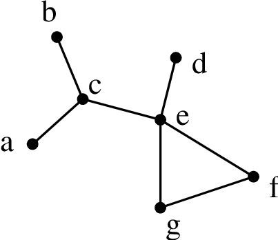
For a given graph, consider the subgraphs that can be obtained by successively removing leaves (nodes of degree 1). The vertex sets of these subgraphs are the closed sets of a convex geometry. The minimal closed set is the 2-core of the graph. Figure 1 shows a specific graph and its lattice of closed sets; for example, the closure of the set is the set .
 |
 |
An extreme point of a set is an element which is not in the closure of . The set of extreme points of is the unique minimal set whose closure is .
2.2 Antimatroids and pruning processes
Next we define antimatroids, which are equivalent to convex geometries. Let be a set, whose elements we regard as letters. A word over the alphabet is called simple if it contains no repeated letters; let be the set of simple words over .
An antimatroid is a pair where is a set and is a set of simple words satisfying:
(L1) If then ; that is, any beginning section of a word of is in .
(L2) If and , then contains a letter such that .
(L3) If and are such that and , then .
Axiom (L1) says that is left hereditary, (L2) is an exchange axiom, and (L3) states that, as we build up a word of from left to right, any letter which can be added to the word at a certain stage can still be added at any later stage.
The supports of the words in are called the feasible subsets of . The feasible subsets determine : a word is in if and only if every initial segment of it is a feasible set. The following theorem provides a one-to-one correspondence between antimatroids and convex geometries.
Theorem 2.2.
[12, Theorem III.1.3] Let be a finite set and be a collection of subsets of . Then is the collection of feasible sets of an antimatroid if and only if is the collection of closed sets of a convex geometry.
By the above theorem, the feasible sets of the antimatroid corresponding to our example of a convex geometry can be read on the descending paths from the top of the lattice of closed sets. A letter corresponds to every edge - this is the element that is removed. Any set of removed elements is the complement of a convex set, thus it is a feasible set. We will see below that the words of the antimatroid can also be read on the descending paths.
An alternative characterization of antimatroids starts by defining a set for every , which is a collection of alternative precedences for ; each precedence is a set not containing . Let be the set of words on the alphabet such that can only appear after at least one of its precedences has appeared:
In the example of Figure 1 the alternative precedences for are , , and . In general, for the process of removing leaves to obtain the -core of a graph, a vertex of degree becomes removable as soon as of its neighbors are removed. Thus its precedences are all the -subsets of its set of neighbors.
A removal process is a procedure in which the elements of a set are removed one at a time according to a given rule. If every element which is removable at some stage of the process remains removable at any later stage, we call this a pruning process.
We are now in a position to explain the correspondence between pruning processes and antimatroids. Given an antimatroid on ground set , we can consider each word of as a removal sequence, which instructs us to remove the elements of from left to right. These removal sequences describe a pruning process: if an element is removable at a certain stage described by word (that is, if ), then one of the alternative precedences of appears in . At any later stage the removal sequence will contain as a prefix, and therefore will contain that alternative precedence for as well.
Conversely, suppose we are given a pruning process on a set . For each element let the alternative precedences of be the subsets such that is removable in . Clearly the antimatroid determined by these sets of alternative precedences consists of the removal sequences in our pruning process.
Example 2.1 gives rise to an antimatroid whose words are the pruning sequences of leaves that one can successively remove from the graph. These correspond to the descending paths from the top of the lattice of closed sets; the word indicates the elements that are being removed as we walk down. For example the leftmost path in the lattice of Figure 1 gives the word , which corresponds to a valid order of successively removing leaves from the graph.
2.3 Circuits and Paths
The circuit description of a convex geometry is a good way to reveal the pruning process which generates it. A rooted set is a set with a designated element called the root. Any collection of rooted sets gives rise to a convex geometry as follows. Suppose is a family of rooted subsets of ; label them where and . Call a subset of full if implies for each ; that is, if the root of a set is never the only element of the rooted set missing from . Say a full set is accessible from if there exists a sequence of full subsets with for each . The following is, in a different language, Lemma 3.7 of [12].
Proposition 2.3.
[12] Let be a collection of rooted sets in . The collection of full subsets of which are accessible from is the collection of closed sets of a convex geometry on .
The set of rooted sets can be interpreted as pruning rules. Let for every , . Then the corresponding pruning process is the one in which an element is removable if and only if at least one element has been removed from each set in .
Conversely, from a convex geometry it is possible to recover a set of rooted sets that generates it. A free set is one of the form . A circuit is a minimal set which is not free, and one can check that each circuit has a unique element which is in the closure of the remaining ones. This element is called the root of the circuit, and is called a rooted circuit.
Even though we will not need this fact, let us point out that the collection of full sets of a family of rooted sets has a nice structure.
Proposition 2.4.
A collection is the collection of full sets determined by a family of rooted sets if and only if it contains and is closed under intersection.
Proof.
First, it is easy to see that the collection of full sets determined by a family of rooted sets contains and is closed under intersection.
Next, suppose is a collection of subsets of that contains and is closed under intersection. We start with being the complete set of rooted sets on . For every remove from all rooted sets , where and . We claim that is the collection of full sets of .
It is immediate by the construction that every is a full set. It remains to show that there are no other full sets. Suppose is a full set for . That means that all rooted sets with and have been removed. In particular has been removed for all . This implies that for every there exists such that and . Since and is closed under intersection, is in . ∎
So far in this paper, rooted sets have played the role of circuits in a convex geometry. It is worth pointing out, however, that one can consider rooted sets as paths which generate a convex geometry in a different way, as follows. Suppose is a family of rooted subsets of which we now call paths; label them where and . Let a subset of be path-full if for every there exists such that . Let it be path-closed if it is path-full, and accessible from by a sequence of path-full subsets with for each . Then the path-closed sets are the closed sets of a convex geometry, and every convex geometry arises in this way from a set of paths.
In this context, the rooted sets can again be interpreted as pruning rules. For every let . Then the corresponding pruning process is the one in which an element is removable if and only if there is a set such that every element of has been removed.
The pruning processes in the literature on random structures are generated by rules for removing elements which can usually be represented in a natural way through circuits or paths. While both points of view are equivalent, sometimes one is more natural than the other. For example, in finding the -core of a graph [25], a vertex becomes removable when at least one element has been removed from every -subset of its neighbors (circuit rule). On the other hand, in the case of identifiable vertices in hypergraphs [6] a vertex is removable if, in at least one of the hyperedges in which it appears, every other vertex has been removed (path rule).
In the rest of the paper, all the rooted sets that appear play the role of circuits.
2.4 Lattices
Finally, we can also think of convex geometries as meet-distributive lattices. A lattice is meet-distributive if for any element the interval is a Boolean lattice, where is the meet of the elements covered by . Meet-distributive lattices are precisely the posets of closed sets of convex geometries. [3, Prop. 8.7.5]
One might wonder whether something more specific can be said about the convex geometries that arise from a set of circuits each of size at most . This question will be particularly natural in Section 4, where convex geometries are applied to the -SAT problem for a fixed value of .
For the situation is very nice. Recall that a lattice is distributive if for any in .
Proposition 2.5.
[12, Cor. 3.10] Let be a set of rooted sets of size 2. The convex geometry generated by these sets is a distributive lattice. Conversely, every distributive lattice arises in this way.
For higher values of , if we start with a collection of rooted circuits of size , the resulting convex geometry generally has additional rooted circuits of different sizes. For the case of , all circuits of the generated convex geometry have size 2. However, for example, the convex geometry defined by the rooted -sets and also has as a circuit.
If we have a bound on the size of the circuits of a convex geometry, we can make the following statement. A lattice is -distributive if for any in .
Proposition 2.6.
[13, Cor. 4.3.] Let be an integer. If all circuits of a convex geometry have size at most , then its poset of closed sets is a -distributive lattice. Not every -distributive lattice arises in this way.
3 Convex geometries as interval partitions of Boolean lattices
In this section we describe our new characterization of convex geometries. We show that convex geometries on a set are characterized by the fact that they induce a certain partition of the Boolean lattice . This partition is encoded in a polynomial identity which, as we will later see, generalizes Theorem 4.2 from [17].
For any collection of subsets of , and a set in , say that an element is excludable from if is in . Let be the set of excludable elements of . When is the collection of closed sets of a convex geometry, is the set of extreme points of .
Theorem 3.1.
Let be a collection of subsets of a non-empty set . The following statements are equivalent:
- 1.
is the collection of closed sets of a convex geometry.
- 2.
As ranges over the intervals partition the Boolean lattice ; that is, for every there is a unique such that .
- 3.
For any collection of and for such that for all , we have
Proof.
1. implies 2. Notice that if is such that , then we have that ; so the only possible choice for is . It remains to notice that, since is the unique minimal set such that , and , it follows that , and therefore .
2. implies 1. We define the map , as follows: for every , let be the unique element such that . We need to show axioms (N1)-(N3) of a convex geometry : is in , is closed under intersection, and every is accessible from .
Axiom (N1) obviously holds, because is in . To show (N3), we show that every set is accessible from any superset that also belongs to . It suffices to prove that there exists an element of that is excludable from . If that were not the case, then , and both of the intervals and would contain , a contradiction.
Finally, we need to prove (N2), which states that is closed under intersection. First we prove the following statement:
If and then .
Suppose that we remove one element at a time from in any arbitrary way, with the restriction that the intermediate sets in the process must all be in and contain . We keep doing this until we cannot continue anymore; suppose the set we obtain is ; by construction, . That means that every element excludable from is in , so . Thus and we obtain the desired statement.
Now suppose and are in . From we obtain that . Similarly , so . But the reverse inclusion holds by definition, so we must have equality. It follows that is in .
2. implies 3. Observe that
Therefore, since for every there is a unique such that , it suffices to prove that for every :
This is easily seen to be true because:
3. implies 2. Consider any set , and let if and otherwise. The equality becomes:
Therefore there is exactly one set for which . ∎
The following corollary gives a characterization of pruning processes among removal processes:
Corollary 3.2.
A removal process on a set is a pruning process if and only if, for each subset of , there is a unique minimal set containing which is achievable by the removal process.
Proof.
As outlined in Section 2.2, a pruning process gives rise to a convex geometry, and in that case is just the convex closure of . For the other direction, let consist of the sets achievable by the removal process; it suffices to show that is the collection of closed sets of a convex geometry. We will show that property 2 of Theorem 3.1 holds. For any set , it holds that , because if there is an excludable element of that is not in , then would not be the minimal set containing . Furthermore, any set for which is a minimal set containing because all of its excludable elements are in . Since there is a unique such set, it is . ∎
We conclude this section by offering a probabilistic interpretation of property 3 of Theorem 3.1.
3.1 A probabilistic interpretation
Let be a convex geometry, and fix with for each element of . Define a probability distribution on the subsets of by independently deleting element with probability and keeping it with probability :
Define a probability distribution on the convex sets of by:
The implication of Theorem 3.1 tells us that is, indeed, a probability distribution. Furthermore, in order to sample from , it suffices to sample from and compute the closure of the obtained set.
Theorem 3.3.
Let be a function defined on the subsets of which depends only on . Then the expected value of when we sample from the distribution on all subsets of , equals the expected value of when we sample from the distribution on the convex sets of .
Proof.
Assuming that , the identity
| (1) |
can be established in exactly the same way as implication of Theorem 3.1. ∎
We note that Aivaliotis, Gordon, and Graveman [2] and Gordon [10] studied the problem of choosing a random subset of a convex geometry under the distribution . They related the expected rank of this random subset to the Tutte polynomial of the antimatroid. In particular, they discovered (1) in a special case which is no simpler than the general case.
The fact that is a probability distribution on is not explicitly stated in [2] or [10], and neither is the probabilistic interpretation of the right hand side of (1). However, these two results follow very easily from that work. Our theorem that the probabilistic property of Theorem 3.3 (or the weaker condition 3 of Theorem 3.1) characterizes convex geometries is new.
4 Convex geometries in the k-SAT problem
Let be a Boolean formula such as
We can assume that is written in conjunctive normal form as a conjunction of certain clauses in the variables and their negations. The Boolean satisfiability problem (SAT) is to determine whether there is some assignment of TRUE and FALSE to the variables which makes the entire formula true. The -SAT problem is the same problem when restricted to formulas with clauses of a fixed size . For there is a polynomial time algorithm for deciding satisfiability, however for the problem is NP-complete.
In their analysis of the Survey Propagation algorithm [19, 4] for 3-SAT, Maneva et al [17] discovered a polynomial identity that holds for any SAT problem and any satisfying assignment. To define this identity first we need to introduce the concept of partial assignments, where to each variable is assigned one of the values or ; the value indicates that a variable is unassigned and free to take either value. Say that a partial assignment is invalid for a clause if plugging into gives either (which makes the clause invalid) or (where the is not free to take either value). A partial assignment is valid for a formula if it is valid for all its clauses. For example, some valid partial assignments for the formula are and , and some invalid partial assignments are and .
Definition 4.1.
Given a Boolean formula , the poset of valid partial assignments is defined by decreeing that covers if is obtained from by switching a or to a .
Figure 2 shows part of the poset of valid partial assignments for the formula above. Note that in this example, somewhat surprisingly, is not greater than in , because to stay valid one must switch and from to simultaneously: and are invalid.

Definition 4.1 suggests that, given a valid partial assignment , we call a coordinate either:
(a) a star ,
(b) unconstrained if and setting keeps the assignment valid, or
(c) constrained if and setting gives an invalid assignment; that is, if is the only satisfying variable in some clause of .
Let , , , and be the sets of star, unconstrained, constrained, and numerical variables of , respectively; so and .
Maneva et al [17] defined the weight of a partial assignment to be
where and are parameters in the interval . They considered the probability distribution which assigns to a probability proportional to for every valid partial assignment . The survey propagation algorithm was then proved to be equivalent to applying the belief propagation marginalization heuristic [24] to this distribution with suitably chosen and . This distribution has the following property, which should not look surprising in view of Theorem 3.1:
Theorem 4.2.
[17] For any satisfying assignment of a Boolean formula and ,
summing over all valid partial assignments which are less than in ; that is, summing over the subposet .
Thus the probability distribution on partial assignments with may be regarded as a “smoother” version of the uniform distribution over satisfying assignments, which corresponds to the case : if we choose a valid partial assignment at random, then the probability of being under is the same for any satisfying assignment . Another consequence of the above theorem is that if the total weight of all valid partial assignments is less than 1, then the formula has no satisfying assignment. In recent work of Sinclair and the second author [18], this fact was used in conjunction with the first-moment method to bound the probability of satisfiability of a random SAT formula with clauses of sizes 2 and 3.
Consider the following experiment:
1. in a valid assignment , change a random unconstrained variable to , and
2. repeat until there are no unconstrained variables.
This procedure has been referred to as “peeling”, “whitening”,
“coarsening” and
“pruning”. We now recognize it as a pruning process on the set
of variables which have numerical values in . At each stage,
we are allowed to remove an unconstrained variable; notice that if a
variable becomes
unconstrained, it remains unconstrained throughout this process.
This experiment is equivalent to taking a random path from down the partial order , by choosing at each step a random partial assignment that is covered by the current one. For a fixed choice of , any such path terminates at the same partial assignment, which is known as a “core”. (Note, however, that different may lead to different core assignments.)
Achlioptas and Ricci-Tersenghi [1] examined the above pruning process and proved that, for and a formula chosen from a particular distribution of interest, there is a high probability that the process will terminate before removing all variables. This is not known to hold for .
With the above description of the removal process, our next result follows easily.
Theorem 4.3.
Let be a SAT formula with variables , and let be a valid (possibly partial) assignment for . Let
Then is a convex geometry. Conversely, every convex geometry arises in this way from a valid assignment for a SAT formula.
Proof.
We show that this statement is equivalent to Proposition 2.3. Consider the clauses of with a unique satisfying variable in , which give when we plug into them. If is the set of variables in such a clause (which must be a subset of ) and is the unique satisfying variable, form a rooted set . Then is clearly the convex geometry generated by these rooted sets. Conversely, given a convex geometry, one can encode its rooted sets into the clauses of a SAT formula with a valid assignment. ∎
The convex geometry corresponding to assignment in Figure 2 is the collection of sets of assigned variables in assignments lying below :
and the words of the corresponding antimatroid can be read out by going down the directed edges; the feasible sets are:
In the particular case of 2-SAT, the convex geometry is very special. By Proposition 2.5, the poset of valid partial assignments is a distributive lattice.
Notice that a SAT formula generally has several different valid partial assignments, and each assignment gives rise to a convex geometry . These different convex geometries fit together nicely, as seen in Figure 2. If and have a non-empty intersection, then their intersection is the convex geometry for the unique element with maximal for which if , and otherwise.
The machinery that we have built up now provides a more illustrative multivariate version of Maneva, Mossel, and Wainwright’s Theorem 4.2 on the probability distribution determined by a SAT problem and a valid assignment . More importantly, in view of Theorem 3.1, it tells us that the identity of Theorem 4.2 holds precisely because a SAT problem gives rise to a convex geometry. Therefore convex geometries are really the context in which this identity should be understood.
Theorem 4.4.
For a valid partial assignment of a Boolean formula with variables , let and denote the sets of star, unconstrained, and constrained variables of in , respectively. Let and be such that for all . Then, for any valid assignment of a Boolean formula ,
summing over all valid assignments which are less than in .
5 Acknowledgments
We would like to thank Elchanan Mossel for posing the question of characterizing the combinatorial objects satisfying Theorem 4.2, and Laci Lovász and Martin Wainwright for helpful discussions. We would also like to thank the referee for very useful suggestions for improving the exposition.
References
- [1] D. Achlioptas and F. Ricci-Tersenghi. On the solution-space geometry of random constraint satisfaction problems. In Proc. ACM Symp. Theory of Computing, 2006.
- [2] M. Aivaliotis, G. Gordon, and W. Graveman. When bad things happen to good trees. J. Graph Theory, 37:79–99, 2001.
- [3] A. Björner and G. Ziegler. Introduction to greedoids. In N. White, editor, Matroid applications, pages 284–354. Cambridge University Press, 1992.
- [4] A. Braunstein, M. Mézard, and R. Zecchina. Survey propagation: an algorithm for satisfiability. Random Structures and Algorithms, 27:201–226, 2005.
- [5] A. Z. Broder, A. M. Frieze, and E. Upfal. On the satisfiability and maximum satisfiability of random 3-cnf formulas. In Proc. ACM-SIAM Symp. Discrete Algorithms, pages 322–330, 1993.
- [6] R.W.R. Darling and J.R. Norris. Structure of large random hypergraphs. Annals of Applied Probability, 15:125–152, 2005.
- [7] R.P. Dilworth. Lattices with unique irreducible decompositions. Ann. Math., 41:771–777, 1940.
- [8] P.H. Edelman and R. Jamison. The theory of convex geometries. Geom. Dedicata, 19:247–274, 1985.
- [9] R. G. Gallager. Low-density parity check codes. MIT Press, Cambridge, MA, 1963.
- [10] G. Gordon. Expected rank in antimatroids. Adv. in Applied Math., 32:299–318, 2004.
- [11] B. Korte and L. Lovász. Shelling structures, convexity and a happy end. In B. Bolobás, editor, Graph theory and combinatorics, Proceedings of the Cambridge Combinatorial Conference in Honor of Paul Erdös., pages 219–232. Academic Press, London, UK, 1984.
- [12] B. Korte, L. Lovász, and R. Schrader. Greedoids. Springer-Verlag, Berlin Heidelberg, 1991.
- [13] L. Libkin. -distributivity, dimension and Carathéodory’s theorem. Algebra Universalis, 34:72–95, 1995.
- [14] M. Luby. LT codes. In Proc. IEEE Symp. Foundations of Computer Science, pages 271–282, 2002.
- [15] M. Luby, M. Mitzenmacher, and M. A. Shokrollahi. Analysis of random processes via AND-OR tree evaluation. In Proc. ACM-SIAM Symp. Discrete Algorithms, pages 364–373, 1998.
- [16] M. Luby, M. Mitzenmacher, M.A. Shokrollahi, D.A. Spielman, and V. Stemann. Practical loss-resilient codes. In Proc. ACM Symp. Theory of Computing, pages 150–159, 1997.
- [17] E. Maneva, E. Mossel, and M. J. Wainwright. A new look at Survey Propagation and its generalizations. J. ACM, 55:2–41, 2007. Extended abstract appeared in Proc. ACM-SIAM Symp. on Discrete Algorithms, 2005, pp.1089–1098.
- [18] E. Maneva and A. Sinclair. On the satisfiability threshold and clustering of solutions of random 3-SAT formulas. Theoretical Computer Science, 2008. To appear.
- [19] M. Mézard, G. Parisi, and R. Zecchina. Analytic and algorithmic solution of random satisfiability problems. Science, 297, 812, 2002. (Scienceexpress published on-line 27-June-2002; 10.1126/science.1073287).
- [20] M. Mézard, F. Ricci-Tersenghi, and R. Zecchina. Two solutions to diluted -spin models and XORSAT problems. J. Stat. Phys., 111:505, 2003.
- [21] M. Mitzenmacher. Tight thresholds for the pure literal rule. Technical Report 1997-011, DEC/SRC, 1997.
- [22] M. Molloy. The pure literal rule threshold and cores in random hypergraphs. In Proc. ACM-SIAM Symp. Discrete Algorithms, pages 672–681, 2004.
- [23] E. Mossel. Personal communication, 2004.
- [24] J. Pearl. Probabilistic reasoning in intelligent systems: networks of plausible inference. Morgan Kaufmann, Palo Alto, CA, 1988.
- [25] B. Pittel, J. Spencer, and N. Wormald. Sudden emergence of a giant k-core in a random graph. J. of Combinatorial Theory, Series B, 67:111–151, 1996.
- [26] J.W. Rosenthal, J.M. Plotkin, and J. Franco. The probability of pure literals. Journal of Computational Logic, 9:501–513, 1999.