Microwave Surface Impedance of Y₁Ba₂Cu₃O_7-δ crystals
Experiment and comparison to a $d$-wave model

Microwave measurements of the surface impedance $Z_{\mathrm{s}}=R_{\mathrm{s}}+\mathrm{i}X_{\mathrm{s}}$ of superconductors are in principle capable of yielding a wealth of precise information regarding the superconducting state, such as the gap parameter, quasiparticle density and nature of scattering. In low $T_{\mathrm{c}}$ superconductors the BCS theory provides a remarkably accurate description of experimental data for $R_{\mathrm{s}}$ and $X_{\mathrm{s}}$ over several orders of magnitude variation, including detailed effects of impurity scattering [1].

Recently, experiments which directly explore the order parameter symmetry suggest a $d_{x^{2}-y^{2}}$ order parameter [2, 3, 4] for high $T_{\mathrm{c}}$ superconductors, although some experiments which suggest a $s$-wave order parameter also exist [5, 6]. It is therefore useful to ask to what extent a $d$-wave model of superconductivity can describe the measured surface impedance of the cuprate superconductors, particularly Y₁Ba₂Cu₃O_7-δ. Some work has been already initiated in this regard [7]. Here in this paper, we present detailed results on the microwave (10 GHz) surface impedance of YBa₂Cu₃O_7-δ crystals. We also compare the complete temperature dependence to numerical calculations based upon semi-microscopic models of $d$-wave and $s$-wave superconductivity, including elastic as well as inelastic scattering effects.

The measurements were carried out in a specially designed, high sensitivity Nb cavity. The method of measuring the surface impedance of superconductors at elevated temperatures using a “hot finger” cavity method was first introduced by one of the authors in reference [8], and the principle has been used in a variety of systems reported in the literature. In the present setup, the Nb cavity is maintained either at $4.2\,{\mathrm{K}}$ or below $2\,{\mathrm{K}}$. The typical background $Q_{b}$ of the cavity can be as high as $10^{8}$. The surface resistance is measured from the temperature dependent Q using $R_{\mathrm{s}}(T)=\Gamma\,\,[Q^{-1}(T)-Q_{b}^{-1}(T)]$ and the penetration depth using $\Delta\lambda(T)=\zeta\,[f(T)-f_{b}(T)]$. The geometric factors are determined by the cavity mode, sample location and the sample size. All measurements were done in the $TE_{\mathrm{011}}$ mode with the sample at the midpoint of the cavity axis, where the microwave magnetic fields have a maximum and the microwave electric fields are zero. The method enables measurement of small crystals and thin film samples.

The crystals were grown in a ZrO₂/Y crucible using highly pure Y₂O₃, BaCO₃ and CuO powders. Crystal growth took place while slowly cooling the melt at a rate of $0.40^{\circ}\mathrm{C/h}$ in the temperature range $970^{\circ}\mathrm{C}$ to $904^{\circ}\mathrm{C}$ and in an atmosphere of $100\,$mbar O₂. After the growth the crystals were annealed in flowing oxygen in the temperature range $600^{\circ}\mathrm{C}$ to $400^{\circ}\mathrm{C}$ during $600\,$h.

We start with an analysis of the normal state properties in the hope to fix some of the normal state parameters which are required for a calculation of the conductivity in the superconducting state. Assuming local electrodynamics, i.e. skin depth limited, the normal state surface resistance $R_{\mathrm{n}}$ is given by $R_{\mathrm{n}}=\sqrt{\omega\mu_{0}\rho_{\mathrm{n}}/2}$ where $\rho_{\mathrm{n}}=\sigma_{0}^{-1}=\mu_{0}\lambda(0)^{2}\,2\Gamma=(ne^{2}\tau/m)^{-1}$. If the classical skin depth limit applies, then the microwave resistivity $\rho_{\mathrm{n}}$ should be the same as the dc resistivity, which is known to be linear. If $\rho_{\mathrm{n}}=\rho_{0}+\gamma T$, then

Figure 1 shows a comparison of the experimental data between $100\,\mathrm{K}$ and $200\,\mathrm{K}$ to the above equation. The data clearly has a sub-linear $T$ dependence, and the fit to eq. (1) is extremely good. From the fit the scattering rate $\Gamma$ can be obtained as

where $\Gamma_{\mathrm{el}}=\rho_{0}/(2\mu_{0}\lambda(0)^{2})$, and $\alpha=\gamma/(2\mu_{0}\lambda_{0}^{2})$. Table 2 gives these parameters for the studied samples under the assumption $\lambda(0)=1400\,\mathrm{\AA}$.

Figure 2 displays the low temperature behavior of $R_{\mathrm{s}}$ for the two samples of Y₁Ba₂Cu₃O_7-δ. Sample B shows a characteristic peak in $R_{\mathrm{s}}$ first reported by [9]. This is not present in sample A, whose behavior is instead closer to that of thin films.

It is evident that the $\lambda$ vs. $T$ data displayed in figure 4 do not show the exponential dependence $\Delta\lambda(T)\propto\exp(-T/T_{\mathrm{c}})$ expected for an isotropic $s$-wave superconductor. Instead the data clearly have a polynomial temperature dependence with a leading linear term [10, 11]. This, together with the nonexponential decrease of $R_{\mathrm{s}}$ at very low temperatures could be taken as indication for $d$-wave pairing.

An important prediction for any superconducting state with nodes in the gap is the presence of a finite residual conductivity $\sigma_{00}$ due to elastic scattering [12, 13]. Its value depends on the particular pair state and, if determined experimentally, could help to identify the type of pairing present. For the $d$-wave state

commonly studied for systems with cylindrical Fermi surfaces of circular cross section one has [12, 13] $\sigma_{00}=ne^{2}/m\pi\Delta_{0}$ at $T=0\,\mathrm{K}$.

This can be related to $\sigma_{\mathrm{n}}(T_{\mathrm{c}})$ by $\sigma_{00}/\sigma_{\mathrm{n}}(T_{\mathrm{c}})=2\Gamma(T_{\mathrm{c}})/\pi\Delta_{0}$. Using the values $2\Gamma(T_{\mathrm{c}})=33\,$meV, and $2\Delta_{0}/{\mathrm{k}}T_{\mathrm{c}}=4.3$ we get $\sigma_{00}/\sigma_{\mathrm{n}}(T_{\mathrm{c}})\sim 1$. Thus the residual conductivity is comparable to the normal state conductivity at $T_{\mathrm{c}}$, which is a surprisingly large value. Note that in BCS the conductivity $\sigma_{1}\rightarrow 0$ as $T\rightarrow 0$.

The relation to $R_{\mathrm{s}}$ is obtained from the limiting result when $\sigma_{2}\gg\sigma_{1}$, whence $R_{\mathrm{s}}(T\rightarrow 0)=\omega^{2}\mu_{0}^{2}\lambda(0)^{2}\sigma_{00}/2$. This can also be written as $R_{\mathrm{s}}/R_{\mathrm{n}}=0.5(\sigma_{1}/\sigma_{\mathrm{n}})/(\sigma_{2}/\sigma_{\mathrm{n}})^{3/2}$. Since the above relationship shows that $\sigma_{1}/\sigma_{\mathrm{n}}\sim 1$, the reduction in $R_{\mathrm{s}}$ from its value at $T_{\mathrm{c}}$ is entirely due to the reduction in $\lambda$ from $\delta_{\mathrm{n}}$ i.e. to the superfluid response. The intrinsic residual surface resistance $R_{\mathrm{s,\,res}}(0)$ which results from $\sigma_{00}$ is much smaller than the value measured for sample B but is compatible with the low temperature data for sample A.

Detailed numerical calculations based on the microscopic models for $s$-wave and $d$-wave superconductivity [14, 15, 16] were carried out.

With suitable choices for the Eliashberg functions it is possible to fit the measured surface resistances within the framework of isotropic strong coupling theory over a wide range of temperature from $T_{\mathrm{c}}$ down to $0.4\,T_{\mathrm{c}}$ [16], highlighting the importance of inelastic scattering processes. This is consistent with earlier measurements over the same temperature range [17]. However at lower temperatures the isotropic gap should make its presence known in the form of an $\exp(-\Delta/{\mathrm{k}}T)$ dependence, which is clearly not observed in either $R_{\mathrm{s}}$ or $\Delta\lambda$.

For this reason we focus in this paper on models of $d$-wave superconductivity, including inelastic scattering. Here we list the main ingredients of the model - details of the model are described elsewhere [16]. A weak-coupling pairing interaction was suitably chosen to give the $d_{x^{2}-y^{2}}$ order parameter $\Delta(T,\pol{k}_{F})$, see eq. (3). The self-consistency equation for the order parameter was solved to give the temperature dependence of the amplitude $\Delta_{0}(T)$, and which is found to be very similar to that for an isotropic order parameter except that $2\Delta_{0}(0)/{\mathrm{k}}T_{\mathrm{c}}=4.29$ rather than $3.52$.

Elastic scattering is parametrized by a normal state scattering rate $\Gamma_{\mathrm{el}}$ and a phase shift $\delta_{\mathrm{N}}$, which can take any value between $0$ (Born approximation) and $\pi/2$ (Unitary limit). Inelastic scattering in the superconducting state is parametrized in the form

with some function $f$ of the reduced temperature $t=T/T_{\mathrm{c}}$.

The inputs to the calculation of the surface impedance $Z_{\mathrm{s}}=(2\mathrm{i}/\sigma_{\mathrm{s}})^{1/2}$ are then $\Gamma_{\mathrm{el}}$, $\delta_{\mathrm{N}}$, $\alpha$, and $f(t)$. In order to fit the steep drop of $R_{\mathrm{s}}$ below $T_{\mathrm{c}}$ we have found it necessary to treat $2\Delta_{0}(0)/{\mathrm{k}}T_{\mathrm{c}}$ as a variable parameter.

The surface impedance is not as sensitive to the choice of model parameters as is the real part of the conductivity $\sigma_{1}$, which is also of some intrinsic interest. Unfortunately, the peak height of the experimentally determined $\sigma_{1}(T,\omega)$ depends strongly on the choice of the zero temperature penetration depth $\lambda(0)$ while the low temperature behavior of $\sigma_{1}$ can be changed substantially by subtracting from the measured surface resistance $R_{\mathrm{s}}$ a residual loss $R_{\mathrm{s}}^{\mathrm{o}}$ [9]. The choice of $R_{\mathrm{s}}^{\mathrm{o}}$ is limited by the consideration that $\sigma_{1}(T=0,\omega)$ should neither be negative nor should it exceed $\sigma_{1}(T_{\mathrm{c}},\omega)$ by a wide margin. With these restrictions we find $R_{\mathrm{s}}^{\mathrm{o}}=0.15\ \mathrm{m\Omega}$ for sample B while for sample A $R_{\mathrm{s}}^{\mathrm{o}}$ is negligible.

The peak heights in $\sigma_{1}$ are reduced when larger values for $\lambda(0)$ are selected. We have chosen $\lambda(0)$ such that the experimental $X_{\mathrm{s}}$ is linear over as large a temperature range below $T_{c}$ as possible. This gives $\lambda(0)=1800\,\mathrm{\AA}$ and $\sigma^{\mathrm{max}}_{1}(T,\omega)=30\,[\mathrm{m\Omega cm}]^{-1}$ for sample A and $\lambda(0)=2000\,\mathrm{\AA}$ and $\sigma^{\mathrm{max}}_{1}(T,\omega)=42\,[\mathrm{m\Omega cm}]^{-1}$ for sample B.

Experimental results for $\sigma_{1}$ are shown in figure 3. In the presence of purely inelastic scattering a peak in $\sigma_{1}$ should occur near $\omega/2\Gamma(T)=1$. This peak is thus expected to shift to higher temperatures as the frequency is increased and to lower temperatures when the overall magnitude $\alpha$ (eq. (2) and (4)) of the scattering rate is increased. For $f(t)=f_{1}(t)=e^{7(t-1)}-e^{-7}$ which has been suggested by Bonn et al. [9] and which is close to the result from the Nested Fermi Liquid model [18, 16], the peak in $\sigma_{1}$ occurs near $10\,\mathrm{K}$ with the peak height greatly exceeding the experimental value. This observation, taken together with the normal state data, shows that elastic scattering needs to be taken into account. When $\Gamma_{\mathrm{el}}$ given in table 2 is used as input parameter, the peak in $\sigma_{1}$ is greatly reduced. In the Born approximation $\sigma_{1}$ rises very steeply from its limiting value $\sigma_{00}$ so that the peak is still located at too low a temperature. In the unitary limit a peak is barely observable. In order to reproduce the experimental results, $\Gamma_{\mathrm{el}}$ has to be chosen much smaller than the analysis of normal state data would suggest. Figure 3 contains a reasonably close fit to the $\sigma_{1}$ data. The fit cannot be improved by varying the phase shift $\delta_{\mathrm{N}}$. Reducing $\delta_{\mathrm{N}}$ from $0.5\pi$ shifts some of the weight of the peak shown in figure 3 to the temperature at which the peak occurs in the Born approximation. At around $\delta_{\mathrm{N}}=0.35\pi$, $\sigma_{1}(T)$ acquires a distinct double peak structure not compatible with the data. We conclude that the phase shift must be close to the unitary limit $0.45\pi\leq\delta_{\mathrm{N}}\leq 0.5\pi$.

The only way to improve the fit would be to choose different temperature dependencies for $\Gamma_{\mathrm{inel}}$ with $f(t)$ decreasing faster then $f_{1}(t)=e^{7(t-1)}-e^{-7}$ for sample B and more slowly for sample A. Even though the two samples differ in oxygen contents (table 1) and by a factor of four in thickness, it does not seem plausible that intrinsic scattering events in the two samples should differ significantly in their temperature dependencies. A more likely source for this discrepancy is a temperature dependence of the “residual” surface resistance $R_{\mathrm{s,\,res}}(t)$. Models have been put forward to explain $R_{\mathrm{s,\,res}}(T)$ by weak links and relate them to $\rho_{0}$ [19].

The theoretical surface resistance for the same model parameters as those used to calculate $\sigma_{1}$ is shown in figure 2. In the case of sample B the phenomenological residual resistance $R_{\mathrm{s,\,res}}(0)=0.15\,\mathrm{m\Omega}$ has been added. Note the intrinsic residual surface resistance in the case of sample A. To fit the data near $T_{\mathrm{c}}$ we had to increase $2\Delta_{0}(0)/\mathrm{k}T_{\mathrm{c}}$ to $6.4$. This is substantially larger than the weak coupling value $4.29$, which has important implications for conclusions regarding fluctuations. The overall fit to the data is very good, showing the same small discrepancies already apparent in figure 3.

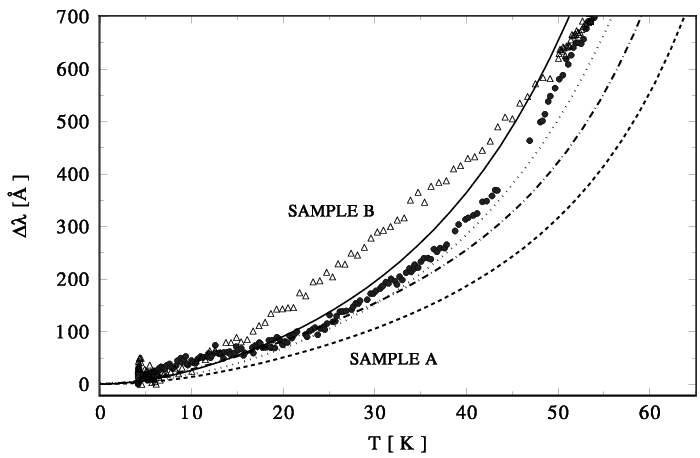
The case for $d$-wave pairing would be strengthened considerably if we could fit the shift in penetration depth equally well using exactly the same model. Experimental and theoretical results are compared in figure 4. Clearly, the agreement is less than satisfactory. Note that the calculated $\Delta\lambda$ is by no means linear, although a polynomial fit in a limited temperature range can certainly be found. The agreement could be much improved by choosing different temperature dependences for $\Gamma_{\mathrm{inel}}$. A good fit for sample A is obtained with $f_{2}(t)=t^{3}$, see figure 4. Decreasing $2\Delta_{0}(0)/\mathrm{k}T_{\mathrm{c}}$ substantially would also improve agreement in the case of $\Delta\lambda$ but would lead to serious discrepancies in the case of $R_{\mathrm{s}}$.

In figure 5 the penetration depth for sample A is plotted over the whole temperature range in the form of the superfluid density $(\lambda(0)/\lambda(T))^{2}$. For such a plot, it is necessary to assume a value of $\lambda(0)$ and this figure shows the variation of $(\lambda(0)/\lambda(T))^{2}$ resulting from different choices of $\lambda(0)$. By varying $\lambda(0)$ one can actually change the sign of the curvature of $\lambda^{2}(T))$ near $T_{\mathrm{c}}$. It is obvious that near $T_{\mathrm{c}}$, since a straight line fits the data pretty well, the behavior is described quite well by a $(1-T/T_{\mathrm{c}})^{1/2}$ dependence, which suggests a mean-field behavior of the order parameter.

Our $d$-wave calculations give a positive curvature for $1/\lambda^{2}(T)$ near $T_{\mathrm{c}}$, indicating a behavior which is slower than mean-field, i.e. $\lambda(T)\rightarrow(1-t)^{\nu}$, where $\nu>1/2$. This is possibly an artifact of the calculation because the total scattering rate (eq. (2)) at $T_{\mathrm{c}}$ is such that $T_{\mathrm{c}}$ should be substantially suppressed according to weak coupling theory. This would lead to noticeably different $T_{\mathrm{c}}$’s for the two samples. Since the $T_{\mathrm{c}}$’s are practically the same, we did not include scattering in the selfconsistency equation. Strong inelastic scattering probably has to be treated within the framework of an anisotropic strong coupling theory, which could also solve the problem of the large value for $2\Delta_{0}(0)/\mathrm{k}T_{\mathrm{c}}$ we had to assume.

In spite of the remaining discrepancies, some of which may be due to contributions from the c-axis conductivity which has not been included in the calculations, d-wave pairing seems to provide an adequate model for understanding features seen in YBa₂Cu₃O_7-δ crystals. The main features of the data appear to be reproduced, although a detailed microscopic justification of the needed parameters is not yet available. We should remark that although we have considered an explicit $d$-wave model, the essential feature is that of nodes in the gap leading to low lying quasiparticle excitations at all temperatures.

This work was supported by NSF-DMR-9223850. We thank M. Osofsky for measurements of the oxygen content of the samples, as well as the organizers of the International Symposium on HTSC in High Frequency Fields held at Cologne, where part of this collaboration was initiated.

References

- [1] S. Sridhar, J. Appl. Phys. 63, 159 (1988).
- [2] D. A. Wollman, D. J. Van Harlingen, W. C. Lee, D. M. Ginsberg, and A. J. Leggett, Phys. Rev. Lett. 71, 2134 (1993).
- [3] C. C. Tsuei, J. R. Kirtley, C. C. Chi, L. S. Yu-Jahnes, A. Gupta, T. Shaw, J. Z. Sun, and M. Ketchen, Phys. Rev. Lett. 73, 593 (1994).
- [4] I. Iguchi and Z. Wen, Phys. Rev. B 49, 12388 (1994).
- [5] P. Chaudhari and S.-Y. Lin, Phys. Rev. Lett. 72, 1084 (1994).
- [6] A. G. Sun, D. Gajewski, M. Maple, and R. C. Dynes, Phys. Rev. Lett. 72, 2267 (1994).
- [7] L. S. Borkowski and P. J. Hirschfeld, Phys. Rev. B 49, 15404 (1994).
- [8] S. Sridhar and W. L. Kennedy, Rev. Sci. Instrum. 59, 531 (1988).
- [9] D. A. Bonn, K. Zhang, R. Liang, D. Baar, and W. N. Morgan, D. C. andHardy, J. Supcond. 6, 219 (1993).
- [10] W. N. Hardy, D. A. Bonn, D. C. Morgan, R. Liang, and K. Zhang, Phys. Rev. Lett. 70, 3999 (1993).
- [11] J. Mao, D.-H. Wu, J. Peng, R. L. Greene, and S. M. Anlage, Phys. Rev. B 51, 3316 (1995).
- [12] P. A. Lee, Phys. Rev. Lett. 71, 1887 (1993).
- [13] P. J. Hirschfeld, W. O. Putikka, and D. J. Scalapino, Phys. Rev. B 50, 10250 (1994).
- [14] K. Scharnberg, J. Low Temp. Phys. 30, 229 (1978).
- [15] R. A. Klemm, K. Scharnberg, D. Walker, and C. T. Rieck, Z. Phys. B 72, 139 (1988).
- [16] C. T. Rieck et al, Intrinsic surface impedance of weak and strong coupling superconductors: Temperature dependent scattering times and anisotropic energy gaps., to be published, 1995.
- [17] S. Sridhar, D.-H. Wu, and W. L. Kennedy, Phys. Rev. Lett. 63, 1873 (1989).
- [18] A. Virosztek and J. Ruvalds, Phys. Rev. B 42, 4064 (1990).
- [19] J. Halbritter, Phys. Rev. B 48, 9735 (1993).