Mirrorless oscillation based on resonantly enhanced 4-wave mixing: All-order analytic solutions
*
Abstract
The phase transition to mirrorless oscillation in resonantly enhanced four-wave mixing in double- systems are studied analytically for the ideal case of infinite lifetimes of ground-state coherences. The stationary susceptibilities are obtained in all orders of the generated fields and analytic solutions of the coupled nonlinear differential equations for the field amplitudes are derived and discussed.
1 Introduction
The possibility to cancel the linear absorption in resonant atomic systems by means of electromagnetically induced transparency (EIT) [1] lead in recent years to fascinating new developments in nonlinear optics [2, 3]. For example coherently driven, resonant atomic vapors under conditions of EIT allow for complete frequency conversion in distances short enough, such that phase matching requirements become irrelevant [4]. Furthermore the large nonlinearities of these systems may lead to a new regime of nonlinear quantum optics on the few-photon level [5, 6] with potential applications to single-photon quantum control [7, 8] and quantum information processing.
One particularly interesting nonlinear process based on EIT is the resonantly enhanced 4-wave mixing in a double- system with counter-propagating pump modes [9]. It has been shown experimentally [10] and theoretically [11, 12] that this system can show a phase transition to mirrorless oscillations for rather low pump powers. Close to the threshold of oscillation an almost perfect suppression of quantum fluctuations of one quadrature amplitude of a combination mode of the generated fields occurs [13, 14]. Also sufficiently above threshold light fields with beat-frequencies tightly locked to the atomic Raman-transition and extremely low relative bandwidth are generated [15].
All previous studies of resonantly enhanced 4-wave mixing were done in the perturbative regime of small amplitudes of the generated fields. In the present paper I want to discuss the case of arbitrary amplitudes. Using a simplified open-system model I will derive stationary propagation equations for the field amplitudes and present analytic solutions of these equations. It will be shown that in an ideal case complete conversion can be achieved within a relatively small interaction length.
2 Model and Atomic Polarizations
I here consider the propagation of four electromagnetic waves in a medium consisting of double- atoms (see Fig.1). These waves include two counter-propagating driving fields with equal frequencies and Rabi-frequencies and , and two probe fields (anti-Stokes and Stokes) described by the complex Rabi-frequencies and , with carrier frequencies and , where is the ground-state frequency splitting. The fields interact via the long-lived coherence on the dipole-forbidden transition between the metastable ground states and . We assume that the driving field is in resonance with the transition, whereas the second driving field has a detuning from the transition. In this case linear losses of the fields due to single-photon absorption processes are minimized.
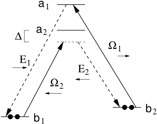
Due to coherent Raman-scattering the pump fields generate counter-propagating anti-Stokes and Stokes fields. For a sufficiently large density-length product of the medium and for a certain pump field intensity, the system shows a phase-transition to self-oscillations [10]. The feedback mechanism required for an oscillation is provided here by the gain medium: A Stokes photon spontaneously generated on the transition propagates in the direction and stimulates the generation of an anti-Stokes photon. This anti-Stokes photon has a different frequency but a fixed relative phase and propagates in the direction. It stimulates the generation of another Stokes photon upstream. The second Stokes photon will be in phase with the first one, provided that the system is approximatly phase matched and that there has been no decay of the Raman coherence. The phase-locked emission of the second Stokes photon then closes the feedback loop. We have shown in [15] that phase-matching enforces a strong pulling of the beat-note of generated and pump fields to the atomic Raman transition. I will therefore assume here that both systems are in perfect two-photon resonance.
In order to calculate the medium response to the fields, one would have to solve the atomic density matrix equations to all orders in all fields taking into account all relaxation rates. Although this is in principle possible it leads to extremely involved expressions. Instead I here use a simplified open-system model which allows to derive rather compact expressions for the atomic susceptibilities.
Since the effects of spontaneous emission are negligible in the present system, we may model all relaxations out of the excited states and by rates out of the system. In thermal equilibrium, i.e. in the absence of all fields, both lower states and are equally populated. I therefore assume – within the open-system approach – that the atoms are pumped into states or with 50% probability respectively. The corresponding rate is denoted as and will later be determined by the requirement that the total probability to find an atom in any of the states is unity. The finite lifetime of the lower-level coherence will here be described by a decay out of all states with rate . Thus the open-system model corresponds to the experimentally relevant situation of an atomic beam or a finite-temperature vapor with time-of-flight broadening. In this case the system can be described by generalized Schrödinger-equations for field amplitudes instead of density-matrix equations.
The interaction Hamiltonian of an atom at position with the fields can be written in the form
| (2) | |||||
If we denote the state vector of the atom as
| (3) |
where are the energies of the corresponding states, we find the following equations of motion of the slowly-varying state amplitudes for an atom at position
| (4) | |||||
| (5) | |||||
| (6) | |||||
| (7) |
Here I have introduced the rates and to distinguish the cases of pumping into () and into (). Note that simultaneously setting corresponds to a coherent preparation of the atoms in a 50–50 superposition of and . In order to describe an incoherent preparation in these levels one has to consider the two cases separately and add the density matrix elements following from both cases.
Solving (4–7) in steady state for the case of injection into , i.e. for and one finds
| (8) | |||||
| (9) | |||||
| (10) | |||||
| (11) |
where I have used that and have kept only the leading terms. Similarly one finds for injection into , i.e. for and :
| (12) | |||||
| (13) | |||||
| (14) | |||||
| (15) |
Taking into account only the leading order contribution in the above expressions is essentially equivalent to assuming an infinitely long lived ground-state coherence between and . In vapor cells with coated walls or by using buffer gases, lifetimes of Hyperfine coherences in alkali vapors in the millisecond regime are possible. Hence neglecting contributions from finite values of seems justified. However, in this case also linear absorption losses are neglected. As a consequence the threshold condition becomes independent on the pump intensity and an arbitrarily small flux of pump photons is sufficient to maintain oscillations [15]. If on the other hand a small but finite ground-state dephasing rate is taken into account, the threshold condition does depend on the pump intensity leading to a lower limit of the pump-photon flux. In the present paper I am interested only in the analytic behavior of the fields in the ideal limit and therefore the small but finite linear losses associated with the ground-state dephasing will be ignored.
The pump rate can be determined from the normalization condition . One finds With this one obtains for the non-diagonal density matrix elements :
| (16) | |||||
| (17) | |||||
| (18) | |||||
| (19) |
The first terms in these expressions describe the nonlinear coupling between the modes and the second ones ac-Stark shift induced changes in the refractive indices. It should be noted that there are no imaginary linear susceptibilities, i.e. there is no linear dissipation despite the fact, that and are in single-photon resonance.
3 Stationary field equations and analytic solutions
In slowly-varying amplitude and phase approximation, the field amplitudes obey the following equation of motion
| (20) | |||||
| (21) | |||||
| (22) | |||||
| (23) |
where , and are the free-space wavenumbers of the generated and pump fields, is the atomic number density and are the dipole moments of the corresponding transitions, which have been assumed to be equal for simplicity. Since the wavenumbers of the fields differ only slightly, one may approximate the coupling parameter in all equations by . Introducing field amplitudes which are slowly varying in space, and one eventually arrives at
| (24) | |||||
| (25) | |||||
| (27) | |||||
| (29) | |||||
| (30) | |||||
| (31) |
where I have dropped the tildes again for notational simplicity, and is the free-space phase mismatch. Expanding these expressions into third order of the generated fields and reproduces the equations of [15]. Equations (25–31) together with the boundary-conditions
| (32) |
where is the length of the interaction region and and are the given input amplitudes, form a nonlinear boundary-value problem. One easily verifies that the set of differential equations has always the trivial solution , and and .
As has been discussed in detail in [15], the phase mismatch is easily compensated in an optically dense vapor by a small detuning from the two-photon resonance. Oscillation occurs at frequencies such that the phase-matching condition is automatically fulfilled. I therefore set this term equal to zero in the following.
3.0.1 Constants of Motion:
The field equations have the following constants of motion. From the energy-momentum conservation follow the Manley-Rowe relations
| (33) | |||||
| (34) |
which state that each photon taken out of the pump fields or is put into the anti-Stokes and Stokes fields and respectively. Furthermore one finds that the total intensity of the pump field is constant in space
| (35) |
The same is true for the generated fields, which however follow already from the above constants of motion.
| (36) |
Without the phase terms in (25–31), which represent contributions due to ac-Stark shifts, also the quartic expression would be a constant of motion. In fact the boundary conditions for the generated fields imply that . It will be shown later on that is in any case to a very good approximation a constant of motion.
3.0.2 Amplitude-Phase Equations:
It is convenient to rewrite the field equations in terms of amplitudes and phases. Introducing and () one obtains
| (37) | |||||
| (38) | |||||
| (39) | |||||
| (40) |
where is the relative phase between the fields. It obeys the equation
| (41) | |||||
| (42) |
3.0.3 Solution for Equal Input Intensities:
Let me now consider the case of equal input intensities of both pump fields, i.e. . Making use of the constants of motion one can write
| (43) | |||||
| (44) |
with the output amplitude of the generated fields and the mixing angle as the only remaining variables. The boundary conditions are now and , if , i.e. for the non-trivial solutions.
Substituting the above expressions into (37) yields the nonlinear equation
| (45) |
where . In order to solve (45) one can in principle introduce a nonlinear stretch of the spatial coordinate according to
| (46) |
which removes the term on the r.h.s. of (45). I will show later on, however, that to a very good approximation . Thus and is used in the following.
Integrating (45) from to leads to an equation for the normalized output amplitude :
| (47) |
where is the complete elliptic integral of the first kind [16]. One easily verifies that (47) has only a real-valued solution , if , which is the threshold condition for mirrorless oscillations [10, 12]. For smaller values of the equations of motion have only the trivial solution.

Figure 2 shows the output intensity of the generated fields normalized to the input intensity of the pump fields as a function of the effective density length product . One clearly recognizes that for a sufficiently large product complete conversion can be achieved.
The spatial behavior of the field strength inside the vapor cell can be obtained from incomplete elliptical integrals following from (45). Figure 3 shows the field amplitudes inside the medium for , i.e. just above threshold and for i.e. for almost complete conversion.

Not to far above threshold, the square root in (45) can be expanded and one recovers the third-order solution obtained in [15]:
| (48) |
with
| (49) |
In order to verify the approximation , I have numerically integrated the differential equation (42) with the above solutions. Figure 4 shows the comparison between the nonlinear coordinate and for the case . One recognizes that deviates from by at most 1%. For smaller conversions an even smaller difference shows up. Therefore the approximation is very well justified. This also implies that is to a very good approximation a constant of motion.

4 Summary
In the present paper all-order atomic susceptibilities for resonantly enhanced 4-wave mixing are presented and field equations derived. The coupled nonlinear differential equations are solved analytically for the case of infinitely long-lived ground-state coherences and under the assumption of negligible phase changes due to ac-Stark shifts. Below a certain critical value of the density-length product only the trivial solution exists, where the generated Stokes and anti-Stokes components have vanishing amplitude. Above the threshold to mirrorless oscillations the photon conversion efficiency increases very rapidly and at a density-length product of about 3 times the threshold value, 95% conversion is achieved.
Acknowledgement
The author would like to thank the organizers of the International Conference on Laser Physics and Quantum Optics, ICLPQO’99, in particular Prof. Shi-Yao Zhu for the invitation and the hospitality in China. The financial support of the German Science Foundation is gratefully acknowledged.
References
- [1] for a review on EIT see: S. E. Harris, Physics Today 50, 36 (1997)
- [2] S. E. Harris, J. E. Field, and A. Imamoğlu, Phys. Rev. Lett. 64, 1107 (1990)
- [3] K. Hakuta, L. Marmet, and B. P. Stoicheff, Phys. Rev. Lett. 66, 596 (1991)
- [4] M. Jain, H. Xia, G. Yin, A. J. Merriam und S. E. Harris, Phys. Rev. Lett. 77, 4326 (1996)
- [5] H. Schmidt and A. Imamoğlu, Opt. Lett. 21, 1936 (1996), A. Imamoğlu, H. Schmidt, G. Woods, and M. Deutsch, Phys.Rev.Lett. 79, 1467 (1997)
- [6] S. E. Harris and L. V. Hau, Phys. Rev. Lett. 82, 4611 (1999)
- [7] S. Harris and Y. Yamamoto, Phys.Rev.Lett. 81, 3611 (1998)
- [8] M. Werner, and A. Imamoğlu, preprint quant-ph/9902005
- [9] P. R. Hemmer, D. P. Katz, J. Donoghue, M. Cronin-Golomb, M. S. Shahriar and P. Kumar, Opt. Lett. 20, 982 (1995)
- [10] A. S. Zibrov, M. D. Lukin, and M. O. Scully, Phys.Rev.Lett. 83 (1999), in press
- [11] M. D. Lukin, P. Hemmer, M. Loeffler, and M. O. Scully, Phys. Rev. Lett. 81, 2675 (1998)
- [12] M. D. Lukin, P. R. Hemmer, M. O. Scully, in Adv. At. Mol. and Opt. Physics, 42B, 347 (Academic Press, Boston, 1999)
- [13] H. P. Yuen and J. H. Shapiro, Opt. Lett. 4, 334 (1979)
- [14] M. D. Lukin, A. B. Matsko, M. Fleischhauer, M. O. Scully Phys. Rev. Lett. 82, 1847 (1999)
- [15] M. Fleischhauer, M. D. Lukin, A. B. Matsko, and M. O. Scully, preprint quant-ph/9907032
- [16] M. Abramowitz and I. A. Stegun, “Handbook of Mathematical Functions”, (Thun, Frankfurt/Main, 1984)