[
Thermal fluctuations in macroscopic quantum memory
Abstract
We describe macroscopic quantum memory devices based on type-II toroidal superconductors and estimate in one case and compute in another the rates at which quantum information stored in these devices “degrades” because of thermal fluctuations. In the case when the entire solid torus is superconducting, the Boltzmann factor in the rate corresponds to a well-defined critical fluctuation, and the rate is suppressed exponentially with the linear size of the system. In the case when superconductivity is confined to the surface of the torus, the rate is determined by diffusive motion of vortices around the torus and does not depend exponentially on the linear size; we find, however, that when the two dimensions of the torus are comparable the rate does not contain the usual volume enhancement factor, i.e. it does not grow with the total surface area of the sample. We describe a possible way to write to and read from this quantum memory.
pacs
PACS: 85.25.Hv, 03.67.Lx PURD-TH-99-07 quant-ph/9909024]
I Introduction
Quantum memory is a device capable of reliably storing linear superpositions of quantum states. It will be a part of quantum computer when (if) that latter is finally built and may be useful for other applications as well. (For a recent review of quantum computing with an emphasis on fault tolerance see ref. [1].)
To work as quantum memory, a physical system must satisfy a number of requirements. First, it must have at least two fairly stable quantum states. These states form a basis for linear combinations that can be stored in the device. For example, the basis may be formed by perturbative quantum states built near local energy minima, and stability of the basis states may be ensured by a large potential barrier separating them. In such cases we will loosely refer to the basis states as the ground states, or vacua, even though these ground states may not be degenerate in energy and in some cases may contain localized excitations. We note, though, that for some purposes it may be desirable to have ground states that actually are (nearly) degenerate in energy. If two basis states and forming a linear combination
| (1) |
are degenerate, the ratio will be preserved by the evolution. When the basis states are not degenerate, the relative magnitude of and will be preserved, but not the relative phase. The relative magnitude, however, can be arbitrary. In comparison, a classical two-state system will only store two values, referred to as 0 and 1.
For long-time quantum storage, one will probably need to build in some redundancy, so that the basis states refer to many microscopic (local) degrees of freedom. However, redundancy is helpful in protecting quantum information only when the local degrees of freedom in the basis states are sufficiently entangled, i.e. the basis states cannot be identified by local measurements. This condition rules out, in particular, any system in which a ground state degeneracy is due merely to spontaneous symmetry breaking by a local order parameter. (To see why, consider an easy-axis magnet, in which magnetization can be in one of two directions. The direction of magnetization can be found by measuring local magnetization in a relatively small region.) The reason why entanglement of local degrees of freedom is necessary for long-time quantum storage is that local measurements will in effect be performed by external noise, and if they can indeed distinguish between the basis states they will destroy the stored quantum information (the Schrödinger-cat scenario).
In a real sample, tunneling transitions between the basis states will cause quantum memory to deteriorate. Nevertheless, if the basis states are sufficiently entangled, tunneling between them will have to involve many local degrees of freedom, and the tunneling probability will be strongly suppressed. Known examples [2, 3] include fractional quantum Hall and similar types of rigid ground states on tori. In these cases, a typical tunneling fluctuation consists of creating a vortex-antivortex pair, transporting the vortex and the antivortex around the torus, along topologically distinct paths, and then annihilating the pair. It has been argued that, at zero temperature, the tunneling probability (and the associated energy splitting between the ground states) is generically of order where is the size of the system, and is some correlation length. So, the zero-temperature tunneling should not be a problem in practice, as long as one can keep the size of the system sufficiently large.
Of more concern are thermal fluctuations. At finite temperature, there will be a sea of vortex-antivortex pairs, with density proportional to , where is the free energy of a single vortex. (This assumes that the temperature is still low enough, so that no phase transition occurs.) One expects that motion of these “preexisting” vortices can effect transitions between ensembles built near different ground states. The question is, then, what is the rate of such transitions, at a given temperature . A single transition is sufficient to destroy the stored quantum information. So, the rate of the transitions will also be the rate at which the quantum information “degrades”, and the corresponding time will be an estimate for the maximal duration of reliable storage.
In this paper, we will compute in one case and estimate in another the rates of finite-temperature transitions between ensembles corresponding to different ground states for some of the simplest systems exhibiting multiple ground states and macroscopic entanglement. One system is a type-II superconducting film grown on the surface of a torus. In Sect. 2 we review the origin of multiple ground states in a type-II superconductor on a torus. The presence of multiple ground states in this case can be seen either via manipulations with vortices and single electrons, which produce a nontrivial phase when transported around each other, or via a semiclassical argument. Transitions between different classical vacua are topological transitions, which change a winding number of the gauge and Higgs fields. In Sect. 3 we construct a correlator that measures the rate of topological transitions at finite temperature. This correlator is analogous to the one proposed in ref. [4] to measure the rate of topological transitions in the electroweak theory. In Sect. 4 we compute the rate. The main ingredient of the computation is that vortices are well separated, and their motion is diffusive, i.e. associated with a large viscosity.
Our main result, for a film of fixed thickness, is that although the rate of topological transitions is indeed proportional to the vortex density, and so is not suppressed exponentially with (the size of the system), there is a power-law suppression. This suppression can be described by saying that there is no volume enhancement of the rate, i.e. as long as the two dimensions of the torus stay comparable, the rate will not grow with the total volume (while the total number of vortices of course will). Equivalently, the rate per unit volume will decrease with the total volume. This absence of macroscopic enhancement is directly related to the diffusive nature of the vortex motion.
It is easy to redesign the device so that the suppression of the finite-temperature rate becomes exponential with . Imagine making the superconducting film thicker, so that vortices resolve into Abrikosov flux lines; the free energy of those grows linearly with their length. In the limiting case, which is the second system we consider, the entire solid torus is superconducting, and a topological transition is mediated by a well defined critical fluctuation—a critical flux line, whose energy is proportional to . The Boltzmann factor in the rate is , where now , so the finite-temperature rate is suppressed exponentially with . The zero-temperature tunneling rate is suppressed even stronger, as an exponential of . So, a solid superconducting torus (or a wire, or a ring, or a hollow cylinder) is a good candidate for stable quantum memory. In the concluding section we discuss a possible way of writing quantum information to and reading it from this device.
We nevertheless retain interest in the two-dimensional case (the film), because a universal quantum computation is theoretically possible with non-Abelian anyons [3], and systems in which those have been argued to occur [5] are two-dimensional. In the concluding section we also discuss whether our results teach us anything about these more complex cases.
II Ground states of a toroidal superconductor
Existence of multiple ground states in a type-II superconductor on a torus can be deduced from the presence of two types of local excitations, vortices and single electrons, with their corresponding values of flux and charge. It can also be obtained from an explicit semiclassical construction of the ground states. In this section, we use the Ginzburg-Landau (GL) theory for description of the ground states. We interpret the GL expression for energy as an effective Hamiltonian for slow degrees of freedom (rather than as a thermodynamic potential, like free energy). So, we treat the GL fields as quantum fields.
The GL Hamiltonian of a superconductor is
| (2) |
where , , and are positive coefficients,
| (3) |
is minus the electric charge of a Cooper pair (), and is the speed of light; everywhere. We concentrate on the extreme type-II case; the corresponding condition on the parameters is
| (4) |
The Hamiltonian of electromagnetic field is taken, for simplicity, in the relativistic form:
| (5) |
In (2), (5) is the complex “order parameter” field (it is not really an order parameter because it is not gauge-invariant [6]), A is the electromagnetic vector potential, E and B are the electric and magnetic fields.
We first consider a superconducting film that extends from to in the direction and is periodic (toric) in the and directions. These periodic boundary conditions define what may be called a “mathematical” torus, as distinct from the surface of a physical torus, a “doughnut”, that one may produce in a laboratory. Later, we will discuss the distinction in more detail and will also consider the case when the entire solid torus is superconducting.
The vortex of the theory (2) is a short (of length ) Abrikosov flux line whose axis is parallel to the axis. A vortex carries magnetic flux of . So, if we break a Cooper pair and transport one of the electrons around the vortex, the wave function of the system will acquire a nontrivial Aharonov-Bohm factor of . As shown in refs. [7], [3], whenever transport of local excitations around each other produces such a nontrivial factor, the ground state of the system on a torus is degenerate, up to an energy splitting decreasing exponentially with the system’s linear size. For the present case, it comes out that the ground state degeneracy on a torus is at least four-fold. We do not reproduce the argument here, as it can be found in the above papers. Besides, in our case the vacuum structure admits a semiclassical interpretation, which allows us to obtain all the requisite results in a different way.
Consider classical vacua of (2), i.e. configurations of the lowest energy. On a torus, these are:
| A | (6) | ||||
| (7) |
where and are arbitrary integers, and are unit vectors in the two directions, and , are the corresponding dimensions of the torus;
| (8) |
The integers and are the winding numbers of the configuration: they count how many times the phase of winds as one travels along the torus’s noncontractible loops. We consider the case when and are comparable and assume, for definiteness, that
| (9) |
i.e. that the larger loop of the torus is in the direction.
Tunneling processes mix the perturbative vacua built near the configurations (6)–(7) into linear combinations, -vacua, analogous to those of the four-dimensional QCD [8]. If we denote the perturbative vacua as , the -vacua are
| (10) |
where and run from 0 to . In this case we need two angles because there are two winding numbers, and . A more important difference from QCD, though, is that in the present case the tunneling amplitudes, and hence the energy splittings among the vacua, are exponentially suppressed with or . This exponential suppression was found in ref. [2] in a slightly different context, see also ref. [3]. It can be explained as follows. A typical tunneling fluctuation consists of a vortex and an antivortex, which travel along topologically distinct routes: the vortex travels distance , and the antivortex distance (if we consider transitions that change ). At least one of these distances is macroscopically large, and to travel that far the object has to move very fast, or to stay in existence for very long, or to achieve a good balance between these two extremes. One finds [2] that even the fluctuation that achieves the optimal balance still has a Euclidean action proportional to , resulting in an exponentially suppressed amplitude.
In what follows we will assume that system is sufficiently large, so that the tunneling processes that change and are practically nonexistent. In this case, the linear combinations (10) are no longer special, and an equally good basis in the ground state subspace is provided by the perturbative vacua built near the classical solutions (6)–(7). From the nontrivial properties of excitations, with respect to transport around each other, we have learned that, when tunneling is neglected, there are at least four degenerate ground states. Now we find infinitely many degenerate vacua . It is easy to make four from infinitely many. Note that the ground states and can be distinguished by breaking a Cooper pair and transporting one of the electrons around the torus in the direction. Say, for the electron will pick no phase factor, while for it will pick a factor of . On the other hand, given that the charge of electron is the minimal charge in the system, there is no way to distinguish between and . Similarly, one cannot distinguish between and . So, in the absence of tunneling, instead of the infinitely many vacua we may as well consider only four “equivalence classes”, corresponding to and both being even, one being even, the other odd, and both being odd, respectively. The four vacua deduced from the quantum numbers of the excitations are representatives of these four equivalence classes.
Although, as we have seen, in the absence of tunneling we do not have to consider the entire infinite “lattice” of the vacua , sometimes it is convenient to do so. In particular, in the next section we will see that thermal fluctuations in the winding numbers are conveniently viewed as diffusion of and over an infinite lattice made by pairs of integers.
Now consider a type-II film that sits on the surface of a solid torus, a “doughnut”, whose bulk is not superconducting. There are still two winding numbers, and . For example, in this case is simply the total magnetic flux through the doughnut’s hole, in units of the flux quantum . One can change to by dragging an extra flux quantum from the outside, through the bulk of the doughnut. This is equivalent to creating a vortex and an antivortex on the outer side of the doughnut, transporting them along topologically distinct paths to the inner side, and annihilating them there, cf. ref. [2]. In quantum theory, this process occurs spontaneously, as a quantum fluctuation. It is a tunneling process between two distinct ground states that differ by one unit of . The conclusion that the tunneling rate is suppressed exponentially with (for transitions that change ) still applies.
One can switch between the ground states “by hand”, i.e. by dragging appropriate fluxes with the help of external solenoids. Switching from to , for a system that was initially in the linear superposition (1), is equivalent to interchanging and . It is hard to say, though, if this “quantum switch” can serve any useful practical purpose.
On a “doughnut”, the superconducting current in a ground state with and is of order , where is the self-inductance of the device: ; in what follows we assume the logarithm here to be of order one. The current density is then inversely proportional to the surface area of the sample. Because the current density is so low, ground states differing by a few units of or are practically indistinguishable with regard to energies of local excitations. This circumstance plays an important role in preservation of quantum coherence at finite temperature.
On the doughnut, as opposed to the “mathematical” torus—a rectangle with periodic boundary conditions, the ground states corresponding to different values of and are not exactly degenerate even in classical theory: for different values of there are different amounts of energy associated with the magnetic field trapped in the doughnut’s hole. This energy has very little influence on the rate of topological transitions, so calculation of the rate can be carried out on the “mathematical” torus. On the other hand, a real device will be a “doughnut”, and in that case the magnetic energy will lead to discrete (labelled by ) energy levels. A resonator tuned to the energy difference between two such levels may then be able to write linear superpositions of quantum states to this device, or to a solid superconducting torus, which we discuss later. Estimates related to this writing technique are given in the concluding section.
III Topological transitions at finite temperature
Consider, for definiteness, two ground states that differ by one unit of and have the same . These states may play the role of the basis states and forming the linear combination (1). When the system is at a finite temperature, excited states are also occupied. For low-lying, perturbative excited states, we can distinguish between states built near , let us call them , and those built near , call them ; we neglect tunneling between these two sectors. It is essential that, for superconducting tori that we consider here, excitation energies are nearly the same for the two sectors, even when (as on a “doughnut”) there is a sizable difference between the corresponding ground state energies. If denotes the energy of , the energy of (), and the excitation energies are, to a good accuracy, equal:
| (11) |
there is a quasiequilibrium state described by the following density matrix:
| (12) |
where
| (13) |
and ; is a normalization factor, and is temperature. This state is no less quantum-coherent than the ground state (1).
The density matrix (12) is not a fully equilibrium one, because it does not include occupation of higher excited states, those that cannot be regarded as being “near” either or . Thermal occupation of these states will determine the rate of transitions between the two sectors. Our goal in this section is to set up formalism for calculating these transition rates. We begin with the case of a type-II film on the surface of a “doughnut”.
Any two configurations that differ by one unit of or one unit of are separated by a potential barrier whose height is, to a good accuracy, twice the energy of a static vortex. In general, a system at finite temperature does not need to tunnel under a barrier; it can go over it as a result of a thermal fluctuation. In many cases, the rate of these thermal transitions can be computed by considering vicinity of the fluctuation corresponding to the top of the barrier [9]. This fluctuation is called the critical fluctuation. For a toroidal type-II film, however, calculational schemes based on expanding near a critical fluctuation are completely useless, for the following reason. The top of the barrier in this case corresponds to a vortex and an antivortex separated by distance (for transitions that change ), see Fig. 1. But at a finite temperature there is a finite density of vortices and antivortices, with a typical distance between them that is much smaller than . In this situation, a pair of widely separated vortex and antivortex cannot have any special significance. Accordingly, we expect that the rate of topological transitions will be determined by motion of vortices already populating the medium. Nucleation and annihilation of vortex-antivortex pairs will merely maintain the equilibrium concentrations of vortices and antivortices.
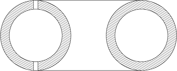
In contrast to the two-dimensional case (film), a critical fluctuation can be readily identified at finite temperature in a solid superconducting torus, or a loop of thick superconducting wire. A solid type-II torus has multiple ground states, although not as many of them as a torus in which superconductivity is confined to the surface. Loops in the direction are contractible through superconductor, so there is no winding number that would correspond to those. But still exists and still counts the number of flux quanta trapped inside the loop. Changing by dragging a flux through the loop is still operational, but instead of a vortex-antivortex pair this procedure now creates one long Abrikosov flux line through the wire’s bulk. The top of the energy barrier is reached when the flux line is along a cross-sectional diameter of the wire, see Fig. 2. The energy of this critical flux line is . The rate of change in via thermal fluctuations is proportional to the Boltzmann factor and thus decreases exponentially with . At zero temperature, when spontaneous topological transitions have to be through tunneling, the suppression is even stronger: a tunneling path is now a worldsheet in the Euclidean spacetime, and the tunneling rate goes as an exponential of .

What we need for the case of a film is a definition of the rate of topological transitions that would make no mention of a critical fluctuation. This requirement is in fact familiar from studies of topological transitions in the electroweak theory, where depending on the temperature one may or may not have a critical fluctuation to expand about. A general definition of the rate in that case is obtained by considering topological transitions as diffusion (or random walk) of the winding number [4]. The rate of the transitions is simply the diffusion rate. Here we construct a similar definition for toroidal superconducting film.
As we already mentioned, to calculate the rate for the film it is sufficient to consider the “mathematical” torus, on which the classical vacua are given by (6)–(7) and are exactly degenerate. To describe diffusion of the winding numbers, we need to generalize their definition so that it will apply away from the vacuum configurations. This generalization is not unique, but the result for the rate will be the same as long as the newly defined winding numbers are equal to and on the classical vacua (6)–(7). A suitable definition is
| (14) | |||||
| (15) |
Note that the winding numbers and are noninteger away from the classical vacua.
Diffusion of , is due to diffusive motion of vortices. We assume that the sample is homogeneous enough so that most of the vortices are not pinned. Translational motion of vortices is semiclassical, so we can define the diffusion rates from the classical equilibrium correlator
| (16) |
and a similar one for . The linear dependence on time on the right-hand side is characteristic of diffusion (in the absence of external forces), and is the definition of the rate. Eq. (16) applies at times large compared to some microscopic time characterizing interactions of vortices with the heat bath.
The precise meaning of the classical averaging in (16) is as follows. For each set of initial conditions (for the full fields A and ), we compute , then evolve the system until time , and compute . The square of the difference is then averaged over all initial conditions, using the Boltzmann distribution for those. At this point, we should remember however that the system (2) is not isolated but evolves under the influence of a heat bath. The heat bath is comprised by all degrees of freedom not explicitly present in (2)—specifically, those associated with electrons. So, the requisite evolution equation includes a random (Langevin) force, and we need to average over realizations of that force as well.
Before we proceed, it is convenient to recast the definition of the rate into a different form, which is more convenient for actual calculation. The procedure is completely standard. First, the left-hand side of (16) is trivially rewritten as
| (17) |
The correlator of time derivatives in (17) is an equilibrium correlator and thus depends only on the difference . We assume that the corresponding correlation time is finite (this assumption can be verified in our specific case). Then, at large the integral (17) is well approximated by
| (18) |
which allows us to rewrite the definition (16) of the rate as
| (19) |
As we will now show, the rate can be found explicitly by a simple calculation based on the picture of diffusing vortices.
IV Calculation of the rate
When a vortex crosses line , the line integral
| (20) |
changes by the amount of the vortex flux, i.e.
| (21) |
the sign depending on which direction the vortex is headed. If a vortex moves the entire length (in the direction), it crosses all such lines and changes , which is essentially the average of over , by . So, if a vortex moves a distance , it changes by the amount
| (22) |
Taking into account all the vortices (of which there are ) and antivortices (of which there are ), we then obtain the time derivative of as follows
| (23) |
We now substitute this expression into the formula (19) for the rate and assume that, because the vortices are well separated, the velocities of different vortices are uncorrelated. We obtain
| (24) |
The correlator of velocities in (24) is computed using the equation of motion for a single vortex. We use a simple Langevin equation of the form
| (25) |
where is the mass of a vortex, in the viscosity coefficient, and is a random force, which we assume to be Gaussian white noise; r is the position vector of the vortex, . The condition of applicability of (25) is that the response of the electronic subsystem to changes in and A is local; otherwise, there would be a nonlocal response kernel instead of the single coefficient . The response is local when the mean-free path of the electrons is much smaller than the characteristic length scale from which receives the main contribution. As we will see in Appendix, the latter length scale is the coherence length of the superconductor , so the condition of applicability of (25) is
| (26) |
i.e. the superconductor should be sufficiently “dirty”.
Calculation of had a long history and has eventually been achieved on the basis of microscopic theory [10]. It is more or less straightforward, though, to obtain an estimate, so we present it here. (We assume that the condition (26) is satisfied.) A moving vortex will constantly transfer parts of its kinetic energy to the electrons, which they will dissipate in collisions with lattice impurities. There are two mechanisms of dissipation [10]. One is Joule heat, which dissipates an amount of energy per unit time per unit volume; here is the normal conductivity of the metal, and is the electric field created by the vortex motion. The other mechanism is related to response of the electrons to changes in the magnitude of ; it dissipates an amount of order , where is the electronic mean-free time, and is the parameter from (2). These two amounts are typically of the same order of magnitude, except at temperatures close to critical, where the second amount is small. We estimate created by a moving vortex in Appendix. This allows us to estimate from
| (27) |
where is the vortex speed. The vortex mass can be estimated from
| (28) |
In Appendix, we find that the integrals in (27)–(28) are saturated at distances from the vortex center. Curiously, in our final formula for the transition rate, and will appear only via the ratio
| (29) |
Note that this ratio grows with , i.e. it is larger in a purer metal (which is still “dirty”, though, in the sense of (26)). Physically, this is because electrons in a purer metal more readily accept energy from a moving vortex.
From (25), it follows that
| (30) |
where , and can be determined by equipartition:
| (31) |
Assembling the pieces together, we obtain
| (32) |
A striking feature of this result is that it does not contain any volume enhancement: although there is a macroscopic factor of , it is essentially canceled out by the inverse powers of . The physical reason behind this suppression is the extremely long time it takes a vortex to circumnavigate the torus: diffusion through a distance of order requires time of order .
The total number of vortices and antivortices is determined by the Boltzmann distribution:
| (33) | |||||
where is the total 2d volume and is the free energy required to create a vortex. Using instead of the vortex energy takes into account thermal population of the vortex’s internal states. Substituting (33) into (32), we finally obtain
| (34) |
This is the rate of transitions that change . The rate of those that change is obtained by interchanging and .
V Discussion
As we have already mentioned, for superconducting film the exponential factor in (34) can be made practically as small as one wishes, because grows linearly with the film’s thickness. So, a thick film on the surface of a torus or, as the limiting case, a solid superconducting torus such as shown in Fig. 2 provide quantum memory that is stable against thermal fluctuations. We propose the following way to write to and read from this quantum memory.
Because magnetic field trapped in the hole of a superconducting torus (or of any other shape with a noncontractible loop) carries energy, the torus behaves as a giant “atom”, in the sense that it has a discrete energy spectrum, with different levels corresponding to different values of . We can write the absolute value of the energy difference between levels with and as
| (35) |
where is of order of the linear size of the system (cf. Sect. 2) and may depend (presumably weakly) on and . (We have restored in this formula.) The corresponding electromagnetic wavelength is
| (36) |
where is the fine-structure constant. For of order of a few cm, and , the wavelength given by (36) is in the millimeter range. It is possible that one will be able to write a linear superposition of quantum states to this device by subjecting it to a pulse of radiation of frequency in a resonant cavity, similarly to how one induces Rabi precession in atoms. One may be able to read from this quantum memory by transferring the linear superposition to radiation field in a high- cavity, as was done for atoms in the experiment of ref. [11]. Unlike a single photon in a cavity or an excited state of an atom, the basis states in our case are macroscopically entangled, so this device will be able to store the linear superposition for a much longer time.
If one wants to operate the read and write cavities at their principal resonant frequencies and use single-photon transitions, at least one of the dimensions of each cavity should be of order . We propose to use, as quantum memory, a loop of superconducting wire, such that the cross-sectional diameter of the wire is of order , while the size of the loop itself is large enough for to be on the order of centimeters. Only short arcs of the loop need to pass through the write and read cavities. This arrangement corresponds to in our formulas. We expect that the effective size of the interaction region, for interaction between cavity photons and the wire, is also of order , and hence of the same order as . In this sense, the interaction is nonlocal, so writing time may be not exponentially large. At the same time, is still macroscopic, so the rate of thermal transitions changing is suppressed.
We leave calculation of the rate of topological transitions induced by a radiation field for future work and turn, briefly, to systems with non-Abelian anyons. Theoretically, a diverse set of manipulations on degenerate states is available for some of these systems [3]. It has been argued that non-Abelian anyons are realizable as excitations of the Pfaffian state [5]. The latter is a quantum Hall state with a certain type of pairing correlation between electrons and is closely related to the state proposed in [12] as a possible explanation of the experimentally observed [13] Hall plateau. With non-Abelian anyons, nontrivial topology is not required for a sample to have degenerate ground states. It is sufficient to “puncture” the surface of the sample with a few localized excitations (vortices). If the typical distance between these vortices is macroscopic, one expects that the zero temperature tunneling between the ground states is suppressed exponentially with [3, 1].
At finite temperature, in addition to those carefully planted vortices there will be a sea of thermally excited ones. What will be the rate at which quantum memory deteriorates in this case? The exponential Boltzmann factor, like the one in (34), should still be present in the rate. In quantum Hall samples will be the larger of the free energy required to create a vortex and the free energy required to unpin it from lattice defects. Because these systems are intrinsically two-dimensional, one cannot increase at will. As an estimate of , we can use the value of temperature corresponding to the onset of strong temperature dependence of diagonal resistivity. This value can be determined experimentally. According to ref. [13], it is 100 mK for the state described in that paper.
The preexponential factor (prefactor) in the rate will be determined by motion of thermally excited vortices around a localized one. By analogy with the results of the present paper, we expect that a thermal vortex that is initially at distance from the localized one will contribute an amount of order to the prefactor. Then, the prefactor will be proportional to
| (37) |
where is either the linear size of the sample or the distance between the localized vortices, so the volume enhancement of the rate will be at most logarithmic.
While this paper was being completed, we have learned about a recent proposal [15] to use, as a basis for quantum computation, current-carrying states in superconducting loops with Josephson junctions. The authors of ref. [15] propose to obtain linear superpositions of these basis states by modulating magnetic fluxes through the loops with pulses of external current. This technique may work also for the quantum memory device proposed here, i.e. one may be able to use an external current instead of a resonating cavity to change . We plan to return to analysis of this possibility elsewhere.
Acknowledgements.
The author thanks T. Clark, S. Kivelson, S. Love, P. Muzikar, and M. Stone for discussions, and N. Giordano for pointing out ref. [15]. This work was supported in part by the U.S. Department of Energy under Grant DE-FG02-91ER40681 (Task B).Electric field of a moving vortex
Electric field produced by a moving vortex determines the vortex mass and the viscosity coefficient . Here we will compute the electric field produced at large distances from the vortex core. We will learn in the process that the region away from the core is not where most of the energy associated with the electric field is concentrated. This precludes us from actually calculating the vortex mass, but we will obtain an order of magnitude estimate.
We begin with a collection of formulas describing a static vortex, in notation close to that of ref. [14]. The magnetic field of the vortex is in the direction. We consider the extreme type-II case when the penetration depth of magnetic field is much larger than the coherence length . For the GL Hamiltonian (2),
| (38) | |||||
| (39) |
When distance from the center of the vortex is much larger than , the magnetic field of a static vortex located at the origin is approximately
| (40) |
where , and is the Macdonald function of the zeroth order. At , this magnetic field satisfies
| (41) |
We also recall that at small values of its argument is logarithmic: .
Now suppose the vortex moves through the origin with velocity v, which lies in the – plane. The rate of change of the magnetic field is
| (42) |
The changing magnetic field produces an electric field, which is related to via one of Maxwell’s equations, . The general solution to this equation in our case is
| (43) |
where is so far an arbitrary function. We fix from the condition that . This condition expresses the absence of charge separation inside the material; we expect it to hold to a good accuracy because charge separation in a metal is associated with a large (plasmon) frequency gap. Using (41), we then obtain, at large distances from the core,
| (44) | |||||
At small , the first term here goes as , but the second term goes as . When the second term dominates, .
Kinetic energy of the vortex is
| (45) |
For the field (44), the integral in (45) diverges at small , due to the singular second term in (44). This means that the main contribution to the mass comes from the core of the vortex, where (44) does not apply. Nevertheless, we can obtain an order of magnitude estimate for the mass by using (44) and cutting of the divergence at distances of the order of the core radius, . This gives
| (46) |
where is the thickness of the film. The second estimate in (46) uses the upper critical field , where is the flux quantum. From eq. (29), we can now obtain an estimate for the viscosity coefficient :
| (47) |
which is in agreement with the results of calculations based on microscopic theory [10].
References
- [1] J. Preskill, quant-ph/9712048.
- [2] X. G. Wen and Q. Niu, Phys. Rev. B 41, 9377 (1990).
- [3] A. Yu. Kitaev, quant-ph/9707021.
- [4] S. Khlebnikov and M. Shaposhnikov, Nucl. Phys. B 308, 885 (1988).
- [5] G. Moore and N. Read, Nucl. Phys. B 360, 362 (1991).
- [6] A good order parameter for superconductor is penetration depth of magnetic field, which is finite in the superconducting phase and infinite in the normal phase.
- [7] T. Einarsson, Phys. Rev. Lett. 64, 1995 (1990).
- [8] C. G. Callan, R. F. Dashen, and D. J. Gross, Phys. Lett. 63B, 334 (1976); R. Jackiw and C. Rebbi, Phys. Rev. Lett. 37, 172 (1976).
- [9] J. S. Langer, Ann. Phys. (N.Y.) 54, 258 (1969).
- [10] For a review and additional references, see A. I. Larkin and Yu. N. Ovchinnikov, in: Nonequilibrium Superconductivity, eds. D. N. Langenberg and A. I. Larkin (North-Holland, Amsterdam, 1986), p. 493.
- [11] X. Maître et al., Phys. Rev. Lett. 79, 769 (1997).
- [12] F. D. M. Haldane and E. H. Rezayi, Phys. Rev. Lett. 60, 956, 1886 (E) (1988).
- [13] R. Willet et al., Phys. Rev. Lett. 59, 1776 (1987).
- [14] E. M. Lifshitz and L. P. Pitaevskiĭ, Statistical Physics. Part 2 (Pergamon, Oxford, 1980).
- [15] J. E. Mooij et al., Science, 285, 1036 (1999).