Unextendible Product Bases, Uncompletable Product Bases and Bound Entanglement
Abstract
We report new results and generalizations of our work on unextendible product bases (UPB), uncompletable product bases and bound entanglement. We present a new construction for bound entangled states based on product bases which are only completable in a locally extended Hilbert space. We introduce a very useful representation of a product basis, an orthogonality graph. Using this representation we give a complete characterization of unextendible product bases for two qutrits. We present several generalizations of UPBs to arbitrary high dimensions and multipartite systems. We present a sufficient condition for sets of orthogonal product states to be distinguishable by separable superoperators. We prove that bound entangled states cannot help increase the distillable entanglement of a state beyond its regularized entanglement of formation assisted by bound entanglement.
I Introduction
One of the essential features of quantum information is its capacity for entanglement. When pure state entanglement is shared by two or more parties, it permits them to send quantum data with classical communication via teleportation [1]. In a more general situation two parties may not start with a set of pure entangled states, but with a noisy quantum channel. To achieve their goal of transmitting quantum data over this channel, they could use an error correcting code [2], or alternatively they can attempt to share entanglement through the channel and later use teleportation. In the latter case, the protocol starts with the preparation of entangled states by, say, Alice, who sends half of each entangled state through the noisy channel to her partner Bob. Since the channel is noisy these states will not directly be useful for teleportation. As a next step Alice and Bob go through a protocol of purification [3]; they try to distill as many as possible pure entangled states out of the set of noisy ones using only local operations and classical communication. We will abbreviate such local quantum operations supplemented by classical communication hereafter as “LQ+CC” operations. Finally, they can use these distilled states to teleport the quantum data. The amount of quantum data that can be sent via the protocol of distillation and teleportation can be higher than by ‘direct’ quantum data transmission using error correcting codes [4]. This has been one of the motivations for studying bipartite mixed state entanglement.
Let us review the definition of entanglement and introduce some notation. A density matrix on a multipartite Hilbert space is separable if we can find a decomposition of into an ensemble of pure product states in . Thus, for a bipartite Hilbert space a separable density matrix can always be written as
| (1) |
where . When a density matrix is not separable, the density matrix is called entangled. In the following we use the notation or to denote the tensor product between a -dimensional Hilbert space and a -dimensional Hilbert space. A Trace-preserving Completely Positive linear map is abbreviated as a TCP map . When a Hermitian matrix has eigenvalues greater than or equal to zero, we denote this as , i.e. is a positive semidefinite matrix. We denote the set of linear operators on a Hilbert space as .
The theory of positive linear maps has turned out to be an important tool in characterizing bipartite mixed state entanglement [5]. It has been shown [6] that all density matrices on which remain positive semidefinite under the partial transposition (PT) map, i.e. , where is matrix transposition [7], are not distillable. We will say that such density matrices have the PPT property or “are PPT”. Here a density matrix is called distillable when for all , there exists an integer and a LQ+CC procedure with , where is a singlet state.
A state which has entanglement but which is not distillable is called a bound entangled state. All entangled states which are PPT are thus bound entangled. But do such states exist? It was shown in Ref. [5] that entangled states with the PPT property do not exist in Hilbert spaces and . The first examples of entangled density matrices with the PPT property in higher dimensional Hilbert spaces were found by P. Horodecki [8]. In Ref. [9] we presented the first method for constructing bound entangled PPT states. This method relies on the notion of an unextendible product basis or UPB. This construction has also led to a method for constructing indecomposable positive linear maps [10]. In Ref. [9] we have given several examples of unextendible product bases, and therefore of bound entangled states. We showed that the notion of an unextendible product basis has another interesting feature, namely the states in the unextendible product basis are not exactly distinguishable by local quantum operations and classical communication. They form a demonstration of the phenomenon of “nonlocality without entanglement” [11].
In this paper we continue the work that was started in Ref. [9]. We will review many of the results that were presented in Ref. [9]. The paper is organized in the following way.
In section II we review some of the definitions and results that were presented in Ref. [9]. In section II.4 we present a first example and indicate a method to make bound entangled states which are based on uncompletable but not strongly uncompletable product bases. In section III we present a sufficient condition for members of an orthogonal product basis to be distinguishable by separable superoperators. In section IV we introduce the notion of an orthogonality graph associated with a product basis; this notion helps us in establishing a complete characterization of all unextendible product bases in . In section V we present unextendible product bases for multipartite and bipartite high dimensional Hilbert spaces. Again we will make fruitful use of the notion of an orthogonality graph. In section VI we report several results that are obtained in considering the use of bound entangled states. We will prove a restriction on the use of bound entangled states in the distillation of entangled states. In section VI.2 we relate the sharing of bound entanglement to the possession of a quantum channel, namely a binding entanglement channel.
II Properties of Uncompletable and Unextendible Product Bases
In this section we exhibit various properties of uncompletable and unextendible product bases, and explore their relation to local distinguishability of sets of product states and bound entanglement.
II.1 Definitions and Counting Lemma
We give the definitions of three kinds of sets of orthogonal product states. First we define an unextendible and an uncompletable product basis:
Definition 1
Consider a multipartite quantum system with parties. An orthogonal product basis (PB) is a set S of pure orthogonal product states spanning a subspace of . An uncompletable product basis (UCPB) is a PB whose complementary subspace , i.e. the subspace in spanned by vectors that are orthogonal to all the vectors in , contains fewer mutually orthogonal product states than its dimension. An unextendible product basis (UPB) is an uncompletable product basis for which contains no product state.
Thus, for an unextendible product basis S, it is not possible to find a product vector in that is orthogonal to all the members in S. For an uncompletable product basis S, it may be possible to find product vectors that are orthogonal to all the states in S, however, we will never be able to find enough states so as to complete the set S to a full basis for .
Now we give the next definition, that of a strongly uncompletable product basis, for which we will use the notion of a locally extended Hilbert space. Let , a Hilbert space of an -partite system. A locally extended Hilbert space is defined as , where is a local extension. When we are given a set of states in we can consider properties of this set embedded in a locally extended Hilbert space .
Definition 2
Consider a multipartite quantum system with parties. A strongly uncompletable product basis (SUCPB) is a PB spanning a subspace in a locally extended Hilbert space such that for all the subspace () contains fewer mutually orthogonal product states than its dimension.
Thus a strongly uncompletable product basis cannot be completed to a full product basis of some extended Hilbert space . In section II.4 we will give an example of a PB that is uncompletable but not strongly uncompletable.
We will review an example of an unextendible product basis of five states in (two qutrits) given in Ref. [9]. Let be five vectors in real three dimensional space forming the apex of a regular pentagonal pyramid, the height of the pyramid being chosen such that nonadjacent vectors are orthogonal (see Fig. 1). The vectors are
| (2) |
with and . Then the following five states in a Hilbert space form a UPB, henceforth denoted Pyramid
| (3) |

To see that these five states form a UPB, note first that they are mutually orthogonal: states whose indices differ by 2 mod 5 are orthogonal for the first party (“Alice”); those whose indices differ by 1 mod 5 are orthogonal for the second party (“Bob”). For a new state to be orthogonal to all the existing ones, it would have to be orthogonal to at least three of Alice’s states or at least three of Bob’s states. However this is impossible, since any set of three vectors spans the full three dimensional space. Therefore the entire four dimensional subspace contains no product state.
We formalize this observation by giving the necessary and sufficient condition for extendibility of a PB (the proof is given in Ref. [9]):
Lemma 1
[9] Let be an orthogonal product basis (PB) spanning a subspace of the Hilbert space of an -partite quantum system with . Let be a partition of into a number of disjoint subsets equal to the number of parties: . Let be the local rank of subset as seen by the th party. Then is extendible if and only if there exists a partition such that for all , the local rank of the th subset is less than the dimensionality of the th party’s Hilbert space. That is to say, is extendible iff .
The lemma provides a simple lower bound on the number of states in a UPB,
| (4) |
since, for smaller , one can partition S into sets of size and thus for all parties.
II.2 Unextendible Product Bases and Bound Entanglement
Every UPB on a bipartite or multipartite Hilbert space gives rise to a bound entangled state which has the PPT property. The construction is the following:
Theorem 1
[9] Let be a UPB in a Hilbert space of total dimension . The density matrix that is proportional to the projector onto ,
| (5) |
is a bound entangled density matrix.
Proof. By definition, contains no product states. Therefore is entangled. If the UPB is a bipartite UPB then we can directly apply the PT map to and find that . Then we use the fact from Ref. [6] that if a bipartite density matrix has the PPT property, it is not distillable. To derive the PPT property of we recall that the PT map is linear so we may apply it separately to the identity and to the projector onto in . The identity is invariant under the PT map. Each projector onto a product state is of the form and as such will be mapped onto
| (6) |
The product states making up the UPB are mapped onto another set of orthogonal product states. Therefore .
In case of a multipartite UPB the PPT condition cannot be used directly. However we can use the above argument to show that under every bipartite partitioning of the parties is PPT. Thus no entanglement can be distilled across any bipartite cut. If any pure ‘global’ entanglement could be distilled it could be used to create entanglement across a bipartite cut. Therefore no entanglement can be distilled and thus the density matrix is bound entangled.
It was pointed out by C.H. Bennett [12] that it is a simple matter to create a set S of nonorthogonal product states in a Hilbert space such that no other product state can be found in that is orthogonal to all the states in S. In fact, except for a set of measure zero, any set of randomly chosen product vectors whose number satisfies Eq. (4) will be unextendible in this sense. For every partitioning the new product vector to be added to the set will have to be orthogonal to other vectors for at least one party . However randomly chosen vectors will typically span a -dimensional space, and therefore such a new product vector that is orthogonal to all the members in the set cannot exist. It is not clear how such a nonorthogonal set of product states could lead to a bound entangled state. The projector on where is now the space spanned by the nonorthogonal product vectors, is entangled, but does not necessarily have the PPT property; in the set of orthogonal vectors obtained by Gram-Schmidt orthogonalization of the nonorthogonal product vectors we might find entangled vectors and therefore might not have the PPT property.
II.3 Local Distinguishability of Product Bases
When two parties Alice and Bob possess one state out of an ensemble of orthogonal product states, we may ask whether it is possible for them to determine exactly which state they have by performing local quantum operations and classical communication. As the states are orthogonal, a joint measurement for Alice and Bob that exactly distinguishes the states is always possible.
In Ref. [9] we found that when a set of product states in a multipartite Hilbert space is strongly uncompletable, it implies that the members in the set cannot be distinguished by LQ+CC. This result is captured in the following lemma:
Lemma 2
[9] Given a set of orthogonal product states on . If the set is exactly distinguishable by local von Neumann measurements and classical communication then it is completable in . If is exactly distinguishable by local POVMs and classical communication then the set can be completed in some extended Hilbert space .
The proof is given in Ref. [9]. We note that in the lemma we only allow POVMs with a finite number of outcomes and we only allow a finite number of rounds of POVM measurements. This restriction comes about because we use Neumark’s theorem [13] to convert a POVM measurement by a party into a von Neumann measurement on a locally extended Hilbert space . When the number of POVM measurement outcomes is infinite, then the extended Hilbert space is infinite dimensional. It is not clear how one can speak of completing a set of states to a full product basis for an infinite dimensional Hilbert space. We avoid the same problem by excluding the possibility for an infinite number of rounds of POVM measurements.
It is possible to strengthen the lemma one step further and include measurements that do not exactly distinguish the set of states, but make an arbitrary small error . By this we mean that we use a measurement and a decision scheme for which the probability of correctly deciding what state the parties were given, is greater than or equal to for all possible states that the parties can possess. When we allow only LQ+CC by finite means, both in space and time, it is possible to prove that when measurement plus decision schemes exist that make an arbitrary small error for all , then there will also exist a scheme that makes no error. The proof of this result is given in Ref. [14] and relies on the fact that the set of measurement and decision schemes is a finite union of compact sets.
We would like to stress that the converse of Lemma 2 does not hold. There do exist sets of orthogonal product states that are not distinguishable by LQ+CC, but which are completable. A prime example is the set of states given in Ref. [11]. For this set it was proved that even by allowing an infinite number of rounds of local measurements, it was not possible to distinguish the members with arbitrary small probability of error.
II.4 Uncompletable Product Bases and Bound Entanglement
Lemma 2 relates uncompletable product bases (UCPBs and SUCPBs) to distinguishability. We may also ask how these (S)UCPBs relate to bound entanglement. First we recall a simple observation that was presented in Ref. [9]:
Proposition 1
[9] Given a PB S on . If the set S is completable in or a locally extended Hilbert space , then the density matrix is separable.
This directly implies that a UPB is strongly uncompletable, since the state corresponding to the UPB is always entangled.
We now ask what properties the projector onto has when S is a UCPB or a SUCPB. Certainly, this projector has the PPT property; it will thus either be separable or have bound entanglement. In order to explore this question, we return to an example that was given in Ref. [9]. We consider the PB Pyr34, a curious set of states in of which the members are distinguishable by local POVMs and classical communication, but not by von Neumann measurements. Pyr34 consists of the states with the states of the Pyramid UPB as in Eq. (2) and defined as
| (7) | |||||
with normalization . Note that (addition mod ). One can show that this set, albeit extendible on , is not completable: One can at most add three vectors like , and . Therefore this set is an example of a UCPB. However it is possible to distinguish the members of this set by local POVM measurements and classical communication. With this property, Lemma 2 implies that the set is completable in a locally extended Hilbert space. The set is thus not strongly uncompletable. This again implies with Proposition 1 that the state is a separable density matrix.
The local POVM that distinguishes the members of Pyr34 starts with a POVM performed by Bob on the four-dimensional side. Bob’s POVM has five projector elements, each projecting onto a vector with , and normalization . Note that is orthogonal to vectors and , or, in general, is orthogonal to (addition mod ). This means that when Bob obtains his POVM measurement outcome, three vectors are excluded from the set; then the remaining two vectors on Alice’s side, and , are orthogonal and can thus be distinguished.
The completion of the Pyr34 set is particularly simple: Bob’s Hilbert space is extended to a five dimensional space. The POVM measurement can be extended as a projection measurement in this five-dimensional space with orthogonal projections onto the states . Then a completion of the set in are the following ten states:
| (8) |
Because the set Pyr34 is uncompletable in the Hilbert space , the state has the notable property that although it is separable, it is not decomposable using orthogonal product states [15]. If it were, those states would form a completion of the set Pyr34.
Let us now take the set Pyr34 and add one product state, say the vector
| (9) |
to make it a six-state ensemble Pyr34+. The density matrix has rank . Is still a separable density matrix? We can enumerate the product states that are orthogonal to the members of Pyr34+, which are not all mutually orthogonal:
| (10) |
These four vectors are not enough to span the full Hilbert space . This means that the range of contains only four product states, whereas has rank 6. Therefore must be entangled. The entanglement of is bound by construction. Since is entangled, Proposition 1 implies that the set Pyr34+ is a SUCPB.
So we have constructed a new bound entangled state whose range is not exempt from product states but has a product state deficit. This set is the first example of a bound entangled state related to a SUCPB, which is not a UPB. Pyr34+ shares with any UPB the fact that its members cannot be distinguished perfectly by local POVMs and classical communication. In conclusion, we have gone from a UCPB Pyr34 to a SUCPB Pyr34+, or from a separable state to a bound entangled state . This construction is an example of a general way to make a bound entangled state from a UCPB:
Lemma 3
Given a UCPB S on there always exists a (possibly empty) set of mutually orthogonal product states orthogonal to S such that when added to S to make , the density matrix is bound entangled.
Proof. We consider the density matrix which is either separable or bound entangled. If it is separable then there exists at least one product state in the range of . We add this state to S and repeat this procedure until the projector onto the complementary subspace of this augmented set is entangled. When S is uncompletable, then we cannot keep adding orthogonal product states: If we would be able to add orthogonal product states until we have a full product basis for , then the set S would be completable on the given Hilbert space , which is in contradiction with S being a UCPB.
The lemma leaves open the possibility that the only bound entangled density matrices we can find are when S has been extended all the way into a UPB. Our example Pyr34+ shows that this is not always the case.
One question of interest which we have not been able to answer is the following: Say we have a PB S which is a SUCPB, but not a UPB, such as the set Pyr34+. Will it be necessary to add more product states to this set as Lemma 3 suggests to make a bound entangled state on the complementary subspace? Or is the state where S is a SUCPB, but not a UPB, always bound entangled?
In the Figures 2 and 3 we show the network of relations that was partially discussed in this section. In section III we will discuss one of these relations, which is the question when orthogonal product states are distinguishable by separable superoperators.
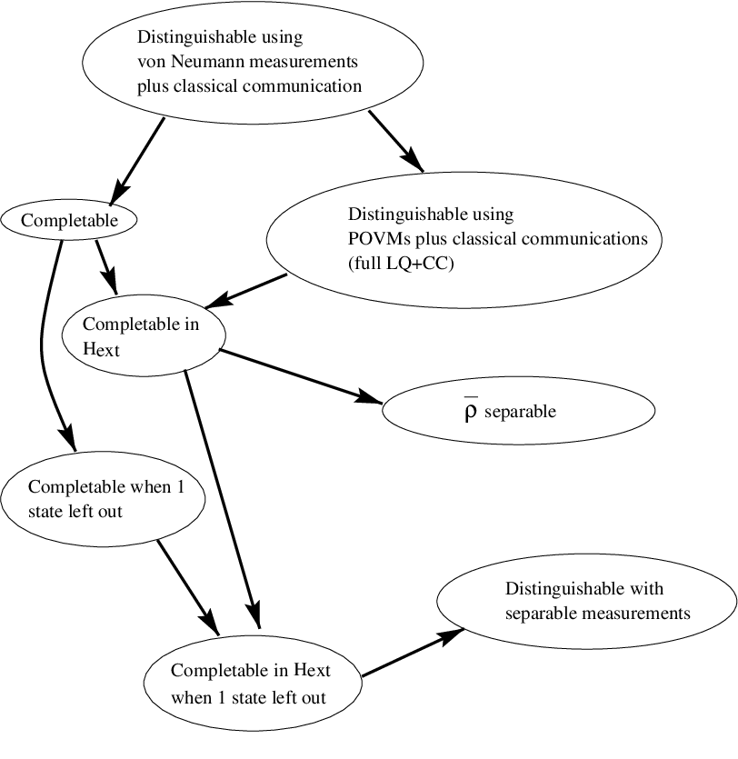

III The Use of Separable Superoperators
In this section we address the question of what kind of measurement does distinguish the members of a PB. We are interested in finding measurements that need the least amount of resources in terms of entanglement between the two or more parties. We introduce a class of quantum operations that are close relatives of operations that can be implemented by local quantum operations and classical communication, the separable superoperators and measurements:
Definition 3
[16] Let . Let . A map is separable if and only if one can write the action of on any density matrix as
| (11) |
where the “operation element” is a matrix and
| (12) |
Similarly, a quantum measurement on a multipartite Hilbert space is separable if and only if for each outcome , the operation elements for all are of a separable form:
| (13) |
Testing whether or not a superoperator is separable is not a simple problem since the operation elements of a superoperator are not uniquely defined. The results of Ref. [11] show that separable superoperators are not equivalent to local quantum operations and classical communication. There is a separable measurement for the nine states presented in Ref. [11]; it is the measurement whose operation elements are the projectors onto the nine states. But the nine states are not locally distinguishable by LQ+CC.
The following theorem gives a sufficient condition under which a set of bipartite orthogonal product states is distinguishable with the use of separable measurements. Unfortunately, it is not known what entanglement resources are needed to implement such separable measurements. They do however form a rather restricted class of operations. Since they map product states onto product states it is not possible to use them to create entanglement where none previously existed.
Theorem 2
Let S be a bipartite PB in with members. If S has the property that it is completable in or local extensions of () when any single member is removed from S, then the members of S are distinguishable by means of a separable measurement.
Proof. Denote the orthogonal rank 1 product projectors onto the states in S as . Let Si, be the set S without a particular state . Since each set Si is completable, the (unnormalized) states
| (14) |
for are separable. Note that . The projectors and for can be made to sum up to the identity by choosing the right coefficients:
| (15) |
using for projectors. Since the projectors are separable, one can decompose them into a set of rank 1 product projectors, labeled by an index . Note that one can choose mutually orthogonal projectors (for a given ) when is completable in the given Hilbert space . When is completable only in a local extension of , these projectors will be non-orthogonal. In both cases the set of product projectors
| (16) |
are the operation elements of a separable measurement. This measurement projects onto states in S or onto product states that are orthogonal to all but one state in S. With a slight modification of this measurement one can construct a measurement which distinguishes the states in S locally. Formally one replaces the projectors of Eq. (16) by
| (17) |
such that the set of states , is an orthonormal set for A and the same for B. This modification leaves Eq. (15) unchanged, so that this new set of operation elements again corresponds to a (separable) measurement. Upon this measurement, however, Alice and Bob both get a classical record of the outcome. If they perform this measurement on states in S, their outcomes will uniquely determine which state in S they were given.
We will show in section IV.1, using the method of orthogonality graphs, that all UPBs in have exactly five members. Theorem 3 (see also section IV) tells us that any set of four orthogonal bipartite product states is completable. Therefore Theorem 2 implies that all UPBs in are distinguishable by a separable measurement.
IV The Orthogonality Graph of a Product Basis
It is convenient to describe the orthogonality structure of a set of orthogonal product states on a multipartite Hilbert space by a graph, which we will call the orthogonality graph of the PB: Essentially the same graph has appeared in a connection with a problem in classical information theory [17].
Definition 4
Let be a -partite Hilbert space with . Let be an orthogonal product basis (PB) in . We represent as a graph where the set of edges have color . The states are represented as the vertices . There exists an edge of color between the vertices and , i.e. , when states and are orthogonal on . Since all the states in the PB are mutually orthogonal, every vertex is connected to all the other vertices by at least one edge of some color.
An example of an orthogonality graph is given in Fig. 4; it is the graph for the bipartite Pyramid UPB. Note that it is also possible to have several edges of different colors between two vertices when states are orthogonal for more than one party.

The representation of a PB in terms of a graph can be useful when we want to determine whether the members of the PB are distinguishable by means of local operations and classical communication. By enumerating the possible orthogonality graphs, it is not hard to prove the following
Proposition 2
The members of any multipartite PB S with three or fewer members are distinguishable by local incomplete von Neumann measurements and classical communication, and the PB is completable to a full product basis.
Proof. We first note that we need only show that the members of S are distinguishable by local von Neumann measurements to also show that S is completable because of Lemma 2. Now, when S has one member, there is nothing to distinguish and the statement is trivial. With two members, the states must be orthogonal for some party and that party can distinguish them. With three members the possible orthogonality graphs are depicted in Fig. 5. We have omitted graphs with multiply colored edges. A multiply colored edge can only make it easier to distinguish the members of the corresponding PB. Thus when a graph corresponds to a distinguishable set after we leave out any multiple coloring, it also corresponds to a distinguishable set with the multiple coloring. We have similarly omitted graphs which are the same as the graphs shown under interchange of parties as clearly those cases will follow the same line of reasoning.

In case (1a), as all the states are mutually orthogonal on Alice’s side, Alice can do a measurement that uniquely distinguishes them. In case (1b) the third state is orthogonal to both state 1 and state 2 on Alice’s side. Therefore Alice can distinguish between and . Then Bob can finish the measurement by telling apart 1 and 2 locally. In case (1c) Alice distinguishes state 2 from state 3, Bob distinguishes 1 from 2, and Charlie distinguishes 1 from 3, together determining the state.
This proposition cannot be strengthened any further: a three party UPB exists with only four members, it is the set Shifts (Eq. (22) and Fig. 8(a)). However, a stronger result may be obtained in the case of a bipartite PB:
Theorem 3
Let be a bipartite PB with four or fewer members, i.e. in any dimension (that allows for this PB). The set S is distinguishable by local incomplete von Neumann measurements and classical communication. The set is completable to a full product basis for .
Proof. We will expand on the proof of Proposition 2. When the set S has one, two, or three members, Proposition 2 applies directly. When S has four members the six possible orthogonality graphs are as given in Fig. 6. Again we omit graphs that are identical to these six under interchanging of parties, and graphs with doubly colored edges.
Case (2a) is trivial. In cases (2b), (2d), and (2e) there is always a state that is orthogonal to all the other states on one side. The measurer associated with that side can then distinguish this state from all the others. The result is that three states are left to be distinguished, which is covered by Proposition 2.

In case (2c) can be distinguished from on Alice’s side after which we are left with two orthogonal states that can be locally distinguished by Bob. In Case (2f) a different type of measurement must be carried out. In the previous cases the measurements were such that none of the states were changed by the measurement. The set of states S was simply dissected in subsets. However, Alice and Bob can carry out a more general type of measurement, namely one that can change the states. Such a measurement must be orthogonality-preserving; by this we mean that the changed states that are left over to be distinguished in a succeeding round must remain orthogonal under the measurement. In case (2f) state 2 is orthogonal to both states 3 and 4 on Alice’s side. Let Alice project with , the projector on the subspace spanned by her side of states 3 and 4, and with , the projector on her side of state 2, and possibly where , and . The projector is only used when the states 2, 3 and 4 do not yet span the full Hilbert space of Alice; if this outcome is obtained, state 1 has been conclusively identified. Otherwise, state 1 is mapped onto or . If the outcome is 2, Bob can finish the protocol by locally distinguishing 1 and 2. If the outcome is 34 we notice that we are in a three state case again and all states are still mutually orthogonal; and state 3 are still orthogonal on Alice’s side as state 3 is invariant under this projection .
These preliminary results will now be used to give a complete characterization of UPBs in .
IV.1 A Six-parameter Family of UPBs in
In Ref. [9] we presented two examples of UPBs in . One is the Pyramid set which was discussed in section II.1 and the second was the set Tiles. The following five states on form a UPB denoted as Tiles
| (18) |
Note that the first four states are the interlocking tiles of Ref. [11], and the fifth state works as a “stopper” to force the unextendibility. The set can be represented with the use of tiles as in Fig. 7. A tile can represent one or more states. For example, the tile in the upper left corner of Fig. 7 represents a state which is of the form
| (19) |
The “stopper” state is not included in the figure; as a tile it would cover the full square.

These two sets, Pyramid and Tiles, are examples of a larger six-parameter family of unextendible product bases in . We will prove that this six-parameter family gives an exhaustive characterization of UPBs in . First we note that five is the smallest number of states in a UPB in , due to Eq. (4).
We will now prove that any UPB with five members on must have an orthogonality graph as in Fig. 4. We will do so by arguing that any vertex must be connected to exactly two other vertices by an edge of the same color. The argument goes as follows. If there exists a vertex that is connected to four other vertices with edges of a single color, then we can locally distinguish this state from the other four states. Theorem 3 implies that we can also distinguish the remaining four states. Now, assume that there exists a vertex, say vertex 1, that is connected to three other vertices, corresponding, say, to the states 2, 3 and 4. Then we can distinguish between 1 and by a local projection that splits state 5 in two projected states. However this projected state 5 is still orthogonal to 1 and . Thus we are left with distinguishing a set of two or four orthogonal product states which can be done locally by Theorem 3.
Finally, it is not hard to see that if all vertices have to be connected to exactly two other vertices, the orthogonality graph in Fig. 4 is the only possible graph.
Now that we have established a unique orthogonality graph, it remains to characterize the solution set. Let , . Let be a set of six angles. We set
| (20) |
with normalizations
| (21) |
We have taken to define the first two vectors of the Alice Hilbert space; the overall phase of and and the phase of the vector are chosen so that , and the first two terms of the above expression for , are real. Also, the overall phase of is fixed so that the coefficient of is real. All the same remarks apply correspondingly to the Bob states. In order for this set of states to be a UPB we require that , , and . If this restriction is made, we see that any set of three different vectors for Alice or for Bob spans a three dimensional space. The Pyramid UPB is obtained from Eq. (20) with the parameter choices , . The parameters for the Tiles UPB are , .
We find that all the solutions having the orthogonality graph of Fig. 4 correspond to UPBs. If we had lifted the restriction on the angles, say, setting , then the set would no longer be a UPB as . At the same time the set would no longer correspond to the graph of Fig. 4, as now state is orthogonal to .
This suggests that UPBs can be characterized by their orthogonality graphs; when a set of states S has an orthogonality graph and S is a UPB then all the sets with graph are UPBs. If this conjecture were true, it would imply that we can classify UPBs by their orthogonality graphs leading to an important simplification. But in section V.3 we present a counterexample to this conjecture for three parties and seven states.
Finally to finish the characterization, we prove that any PB with six or more members in is completable. We give the proof excluding a six member UPB in Appendix A. The density matrix of a PB with seven or eight states has rank two and rank one respectively. By construction this density matrix is either a bound entangled state or a separable state, as follows from Theorem 1. It can be shown by different arguments that there exists no bound entangled state with rank less than or equal to two [18]. The state must therefore be separable. To the seven state PB we therefore can add a product vector to make it an eight state PB which is again extendible.
V Multipartite and high dimensional bipartite UPBs
In this section we introduce several examples and families of UPBs. In section V.1 we present UPBs on multi-qubit Hilbert spaces. In section V.2 we give two constructions of high dimensional bipartite UPBs based on tiling patterns such as in Fig. 7. In section V.3 we give multipartite UPBs based on a generalization of the orthogonality graph of the Pyramid UPB (Fig. 4). In section V.4 we present a bipartite high dimensional UPB which is based on quadratic residues. Finally, in section V.5 we prove that tensor products of UPBs are again UPBs.
V.1 GenShifts and other UPBs in qubit Hilbert spaces
We first give a theorem that was proved in Ref. [9]:
Theorem 4
[9] Any set of orthogonal product states in for any is distinguishable by local measurements and classical communication and therefore completable to a full product basis for .
Even though any bipartite product basis involving a qubit Hilbert space is completable, we found in Ref. [9] that a tripartite UPB involving three qubits is possible. This was the set Shifts given by the states
| (22) |
It follows from Theorem 4 that when we make any bipartite split of the three parties, say we join parties BC, that the set Shifts is completable to a full product basis for . Thus the bound entangled state that we construct from Shifts as in Eq. (5), must be separable over any bipartite split. Therefore this bound entangled state could have been made without any entanglement between A and BC, or AB and C, or C and AB. However, the state is entangled. One may say that the entanglement is delocalized over the three parties.
Our construction of Shifts can be generalized to multipartite UPBs, which we will call GenShifts. Again, because of Theorem 4, the bound entangled states based on GenShifts have a form of delocalized entanglement. The bound entangled states could have been made without entanglement between any single party and all the other remaining parties. We do not know whether the bound entangled states are separable over a split in two or more parties and all the other parties.
GenShifts is a UPB on with members, the minimal number for a UPB, Eq. (4). The first state is . The second is
| (23) |
The states and for all are chosen to be neither orthogonal nor identical. Also, is neither orthogonal nor identical to the state for all . The other states in the UPB are obtained by (cyclic) right shifting the second state, i.e. the third state is
| (24) |
These states are all orthogonal in the following way: The state is special and it is orthogonal to all the other states as they all have a for some party. Leaving this special state aside, all states are orthogonal to the next state, their first right-shifted state, by the orthogonality of and . All states are orthogonal to the nd right-shifted state by the orthogonality of and . The rd right-shifted state is made orthogonal with and . We can continue this until the last th right-shifted state and we are done.
As there are no states repeated on one side of the UPB all sets of two states span a two dimensional space; Lemma 1 implies that the set is a UPB.
The orthogonality graph for the first example of GenShifts which is just the set Shifts, is shown in Fig. 8(a). For and , the graph for GenShifts is the only orthogonality graph possible for a UPB in this Hilbert space. For graphs other than the one corresponding to GenShifts are possible. It is simple to argue that, as in the UPB (section IV.1), all PBs having the GenShifts orthogonality graph are UPBs: The orthogonality graph of GenShifts is partially characterized by the fact that there is only one edge emanating from every vertex of a particular color. This implies that no states in a set corresponding to this orthogonality graph are repeated, that is, the same state for a party is not used more than once in the set. As the set is minimal, this implies that such an orthogonality graph directly fulfills the conditions of Lemma 1; every pair of two states spans a two dimensional space. Also, when we consider a minimal PB (having members for parties) and its orthogonality graph has a doubly colored edge, then the PB cannot be a UPB. This is because the property of having a doubly colored edge directly translates into some pair of states not spanning a two dimensional Hilbert space.

Using the orthogonality-graph construction, we can prove that if the number of parties is even, then qubit UPBs with states, the minimal possible number by Lemma 1, do not exist. We show this by demonstrating that some states would have to be repeated; but repeated states permit a partitioning as in Lemma 1 which allows the introduction of another orthogonal product state. Fig. 8(b) illustrates the idea: Considering the lines of just one color, we note that two cannot emanate from the same node (otherwise there would be a repeat), but after joining them up pairwise there will be one left over, since the number of states is odd. But since this last node has no lines of the first color coming into it, it will have to have at least two of some other color emerging from it, which would again force a repeat. Therefore, the basis would be extendible.
V.2 GenTiles
We introduce a bipartite product basis GenTiles1 in where is even. These states have a tile structure which in the case of is shown in Fig. 9. The general construction goes as follows: We label a set of orthonormal states as . We define the set of ‘vertical tile’ states
| (25) |
where . Similarly, we define the set of ‘horizontal tile’ states:
| (26) |
Finally we add a ‘stopper’ state
| (27) |
The stopper state is not depicted in Fig. 9; as a tile it would cover the whole by square. The representation of the set as an arrangement of tiles informs us about the orthogonalities among some of its members. It is not hard to see that nonoverlapping tiles are orthogonal. The orthogonality of the states and for follows from the identity
| (28) |
With the same identity we can prove that the states and for are mutually orthogonal. Finally, every state or is orthogonal to the ‘stopper’ as
| (29) |
and . The set has states, much more than the minimum number in a UPB on , which is . We can prove that this construction is a UPB in and by exhaustive checking of all partitions (see Lemma 1). This procedure is hard to implement computationally for arbitrary high dimension, but one may conjecture (and prove, see Ref. [20]) that
Theorem 5
The set of states GenTiles1 form a UPB on for all even .

Another tile construction which we call GenTiles2 can be made in dimensions for , and . The construction is illustrated in Fig. 10. The small tiles which cover two squares are given by
| (30) |
These short tiles are mutually orthogonal on Bob’s side. The long tiles (in general not contiguous) that stretch out in the vertical direction in Fig. 10 are given by
| (31) |
with . Lastly we add a ‘stopper’ state
| (32) |
The total number of states is .

We can show that these states form a PB. For the states and are orthogonal on Alice’s side. We also have
| (33) |
The states and with and are orthogonal on Alice’s side. The long tiles are constructed such that they are orthogonal to the states and on Bob’s side, see Fig. 10. Therefore is orthogonal to and . The states are orthogonal to the stopper on Alice’s side. Finally, the states are orthogonal to as
| (34) |
and . We conjecture that this PB GenTiles2 is a UPB (the proof of the conjecture has been given in Ref. [20])
Theorem 6
The set of states GenTiles2 form a UPB on for , and .
Note that GenTiles2 with does not form a UPB.
V.3 Sept and GenPyramid
Let us first consider a generalization to . Define the following states
| (35) |
with and . The following seven states in form the UPB Sept
| (36) |
The orthogonality graph of these vectors is shown in Fig. 11. To prove that these states form a UPB, we must show that any subset of three of them on one of the three sides (Lemma 1) spans the full three dimensional space. As the vectors form the apex of a regular septagonal pyramid, there is no subset of three of them that lies in a two dimensional plane. It is not known whether the complementary state is separable over bipartite cuts, as with (see Eq. (22)), or whether it is a bound entangled over the bipartite cuts.

This construction can be extended to , the minimal UPB thus constructed we will call GenPyramid. We have parties and states where is a prime number. Thus one can have , etc. The states in the polygonal pyramid with vertices are defined as
| (37) |
In Sept and Pyramid, was chosen such that nonadjacent vertices were orthogonal. For larger primes one has to make a choice of which vectors to make orthogonal that depends on : in order for the vectors and to be made orthogonal by lifting these vectors out of the plane of the polygon, we must have
| (38) |
i.e. the angle between the vectors in the plane must be larger than 90 degrees. One can always find such an given a , for example, for , or 3. With the choice of one fixes and as
| (39) |
Finally, the UPB GenPyramid is
| (40) |
The primality of ensures that there are no states repeated on one side: there is no in the range such that for some integers if is prime. Orthogonality is also ensured by primality. As in Fig. 11 there will be a party for whom next neighbor states are orthogonal, there will be a party for whom all second neighbor states are orthogonal, etc. up to the th neighbor. This implies that all vertices in the orthogonality graph are mutually connected (orthogonal), so the orthogonality graph is complete. From basic three dimensional geometry it follows that any set of three vectors has full rank when and thus these generalized sets form UPBs .
It was noted by A. Peres [21] that this construction is quite general: instead of the vectors of Eq. (37), we take any set of vectors such that and such that any triplet of vectors with spans the full three dimensional space. We construct the vectors as in Eq. (40) with , with given in Eq. (38). This set can form a UPB. But in this more general construction a more complete check is required to make sure that any three different vectors are linearly independent. If we restrict ourselves to just requiring that adjacent vectors be orthogonal, we find that there are sets with the same orthogonality graph as, for example, Sept, but which are not UPBs. An example of such a set is the following:
| (41) |
For these states we have and no other states are orthogonal. We can construct a PB by replacing the states in Eq. (40) by these vectors . This PB has the same orthogonality graph as Sept. However, the vectors and lie in a two dimensional plane. This implies that we can add a new product vector to the PB thus constructed. This provides the counterexample to the idea that there is a straightforward correspondence between orthogonality graphs and UPBs.
V.4 UPBs based on quadratic residues
QuadRes is a family of UPBs, which are based on quadratic residues [22]. The UPB is a set of orthogonal product states on where is such that is a prime of the form . The set contains members, which is the minimal number for a UPB . Thus we can have , etc. The first triple is the Pyramid UPB.
Let be . Let be a group of quadratic residues, that is, elements such that
| (42) |
for some integer . is a group under multiplication. The order of the group is . The following properties hold: when and , a quadratic nonresidue, then . Also, if and , then [22]. The states of the UPB are
| (43) |
where
| (44) |
where is a real normalization constant to be fixed for orthogonality and are unit vectors of the form , etc. The dimension of the Hilbert space is , one more than the order of . One can prove that these vectors can be made orthogonal by an appropriate choice of , for :
| (45) |
One uses the properties of to find that for :
| (46) |
Thus the orthogonality relation of Eq. (45) for is of the form
| (47) |
where
| (48) |
The value of as a function of () only depends on whether , because of the group property of . Call this value when . Then when , because of Eq. (46). Finally we also need to establish that is real. One considers in which one sums over . As and when is of the form (see Theorem 82, [22]), . Thus . Both for negative as well as positive , Eq. (47) has a solution for , and thus Eq. (45) is satisfied for all .
Theorem 7
Proof. The proof requires the application of Lemma 1, that is, one must show that any set of states on either side spans the full -dimensional Hilbert space. To do this, we need to show that any subset of of the vectors defined in Eq. (44) has full rank. Checking whether a subset of these has full rank is easily seen to be equivalent to checking whether the determinant of a matrix does not vanish, where is the matrix whose entry is , being the ’th element of the set and the ’th element of the set . However, a theorem of Čebotarev [23] shows that the matrix is of full rank for any two arbitrary sets , subsets of , proving Theorem 7.
Drawn as orthogonality graphs as in Fig. 4, these UPBs are regular polygons, with a prime number (of the form ) of vertices. The elements of the quadratic residue group correspond to the periodicity of the vectors that are orthogonal on one side. For example, when , one has quadratic residues and . Thus on, say, Alice’s side, every vertex is connected to its first neighbor (1), every vertex is connected with the rd neighbor (3) etc. On Bob’s side the orthogonality pattern follows from the quadratic nonresidues.
V.5 Tensor powers of UPBs
When we have found two UPBs, we may ask whether the tensor product of them is again a UPB. The answer is yes, as indicated by the following theorem:
Theorem 8
Given two bipartite UPBs with members , on and with members , on . The PB is a bipartite UPB on .
Proof. Assume the contrary, i.e. there is a product state that is orthogonal to this new ensemble which we call . The idea is to show that this leads to a contradiction and thus PB2 is a UPB.
Note first that for any UPB a partition into a set with 0 states for Bob and all states for Alice gives rise to a (see Lemma 1); the states on Alice’s side together must span the entire Hilbert space of Alice. Also note that if one takes a tensor product of two UPBs (defined on and ) this partition in which all states are assigned to Alice still leads to .
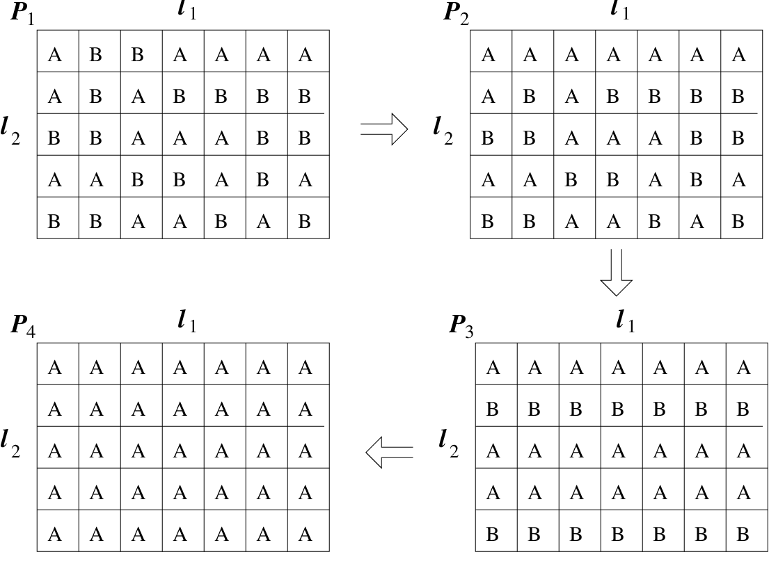
The set PB2 has members. The new hypothetical product state to be added to the set has to be orthogonal to each member either on Bob’s side or on Alice’s side, or on both sides. One can represent this hypothetical orthogonality pattern as a rectangle of size (number of columns) by (number of rows) filled with the letters A and B, depending on how the new state is orthogonal to a member of the PB2. This is illustrated as partition in Fig. 12. When the hypothetical state is orthogonal on both sides, we are free to choose an A or B in the corresponding square.
Consider a row of this rectangle, for example the first one. The pattern of As and the Bs can be viewed as a partition of the UPB and therefore one knows that one of these sets, either the A or the B set, must have full local rank. But if the A set is the one with full local rank, then the state is also orthogonal to PB2 with respect to partition (Fig. 12) in which the whole row is filled with As. This is so since the local rank is not changed (because the A rank was already full for the row) and the rank cannot increase (since states are removed from the B set). This is true for every row in turn, which leads us to partition . Then doing the same to columns, since all columns are identical they will all be full rank for either A or B, so we will obtain the unanimous partition . This partition however contradicts the fact that both sets were UPBs.
The theorem has the consequence that arbitrary tensor powers of bipartite UPBs are again UPBs. A generalization of the theorem for multipartite states is true as well; in the proof we replace A/B partitions with partitions of As, Bs, Cs etc.
VI The Use of Bound Entanglement
It has been shown [24] that bound entangled PPT states are not a usefull resource in the teleportation of quantum states. On the other hand it has also been shown [25] that bound entangled PPT states can have a catalytic effect in the (quasi) distillation of a single entangled state. In the next two sections we discuss the use of bound entangled states: in a protocol of distillation of mixed entangled states and in defining a binding entanglement channel.
VI.1 Distillation of Mixed Entangled States
We will prove that bound entangled states cannot be used to increase the distillable entanglement of a state beyond its regularized entanglement of formation assisted by bound entanglement . By a bound entangled state we mean a state that cannot be distilled, i.e. if we are given many copies of this density matrix we cannot distill any pure entanglement out of this set. These set of states includes the bound entangled PPT states and also possibly some NPT entangled states [26, 27].
We denote the density matrix of a set of pure EPR pairs or other maximally entangled states as . The precise definition of distillable entanglement uses a limit in which the number of copies of the state to be distilled goes to infinity while at the same time the fidelity of the distilled states with respect to a maximally entangled state goes to 1. In the notation we use here we omit these limits for the sake of clarity. We refer the reader to Ref. [28] for a treatment and discussion of various equivalent definitions of distillable entanglement.
We start with the following lemma:
Lemma 4
For no integer and bound entangled state does there exists a LQ+CC TCP map such that
| (49) |
Proof. Suppose Eq. (49) were true. Expanding the density matrix proportional to the identity on the dimensional Hilbert space, we obtain
| (50) |
By the linearity of it follows that
| (51) |
The fidelity of the output state in Eq. (51) with respect to is . If the output is projected into the Hilbert space of dimension is inhabited by the term of Eq. (51) this fidelity can only increase or remain the same. It has been shown by Horodecki et al. [29] that a state for which is distillable, so the output state is distillable (as ). But this is a contradiction, since the input state of Eq. (51) has only bound entanglement, and the TCP map is LQ+CC and therefore it cannot create any free entanglement. This proves that such an LQ+CC does not exist.
Lemma 5
For no integer and bound entangled state and does there exists a LQ+CC TCP map such that
| (52) |
Proof. If existed, iterated application of it times would produce the map of Lemma 49. However this cannot exist and therefore does not exist.
The distillable entanglement of a state assisted by bound entanglement, , is defined by optimizing over all LQ+CC TCP maps and bound-entangled states and values for such that
| (53) |
Proposition 3
, where () is (the -assisted) regularized entanglement of formation of .
Proof. The BE-assisted regularized entanglement of formation of a density matrix is defined by the optimal LQ+CC TCP map and optimal choice for and such that
| (54) |
Suppose . This leads to a contradiction, because the composed map
| (55) |
cannot exist by Lemma 52.
These results also provide some partial answers to the questions raised in the discussion of Ref. [30]; it bounds the use that bound entanglement can have in the distillation of mixed states. The result does leave room for nonadditivity though; for states which have it could still be that .
VI.2 Binding Entanglement Channels
As noted independently by Horodecki et al. [30], there exist quantum channels through which entanglement can be shared, but only entanglement of the bound variety. These binding entanglement channels are discussed in Ref. [30]. Here we present a simple physical argument for their existence based on bound entangled states, both of the PPT kind as well as the NPT kind (if these exist, see Ref. [26]).
Consider any bound entangled (BE) state on . With this state we define a channel which takes an -dimensional input and measures it, along with one half of , in a basis of maximally entangled states. The output of the channel is the other half of and the classical result of the measurement, see Fig. 13(a). It is easy to see that no pure entanglement can ever be shared through such a channel, as any procedure which could would also be able to distill entanglement from the BE state itself. No pure entanglement can ever be shared through such a channel, since any procedure which could would also be able to distill entanglement from the BE state itself: If Alice and Bob share many copies of , they can simulate actually having the channel by having Alice measure each of her inputs to the channel along with her half of a copy of in the basis of maximally entangled states, and telling Bob the classical result, just as the channel itself would have done. By plugging their simulated channel into a procedure that could share pure entanglement through the channel, Alice and Bob would have distilled entanglement from the bound entangled state .
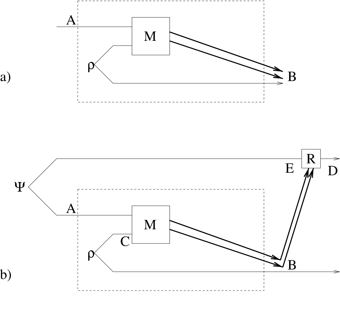
This does not yet establish the existence of a BE channel as our channel might only be able to share separable states. Now suppose Alice, whose lab is at the top of Fig. 13(b), creates a maximally entangled state in and sends half of it into the channel. Bob, whose lab is at the bottom right of the figure, sends the classical output data to Alice, who does some unitary operation R depending on those data. If the set of possible R’s is chosen correctly, the result is precisely quantum teleportation [1] of the half of at point C to point D. So a bound entangled state has been shared through the channel. Finally, we note that the actual transmission of the classical data from Bob to Alice, while a simplifying idea, is not strictly needed. That communication along with rotation R is a LQ+CC operation and therefore cannot create entanglement where there was none. So even before the classical communication the state shared between points B and E must have been bound entangled.
VII Conclusion
We have shown some of the mathematical richness of the concept of unextendible and uncompletable product bases, their relation to graph theory and number theory. By exhibiting some of this structure we have uncovered a large family of bound entangled states. We have presented the first example of a new construction for bound entangled states. It would be interesting to try to understand the geometry of uncompletable product basis in a more general way; some of the interesting open questions in this respect have been mentioned in the paper. For example, from every multipartite UPB we can derive bipartite PBs by considering the UPB over bipartite cuts. Do these PBs have any special properties; can they correspond UCPBs when the local Hilbert spaces have dimension more than 2?
The question that this work only partially addresses is one concerning the fruitful use of bound entangled states and the resources needed to implement separable superoperators. Further investigations into this matter will be worthwhile.
Acknowledgements. Part of this work was completed during the 1998 Elsag-Bailey-I.S.I. Foundation research meeting on quantum computation. We would like to thank Charles Bennett, Asher Peres, Danny Terno, Ashish Thapliyal and John Tromp for discussion. We would like to thank Noga Alon for bringing Čebotarev’s theorem to our attention, thus proving Theorem 7. JAS and DPD acknowledge support from the Army Research Office under contract number DAAG55-98-C-0041. The work of TM was supported in part by grant #961360 from the Jet Propulsion Lab, and grant #530-1415-01 from the DARPA Ultra program.
Appendix A No six member UPB in
In this appendix we prove that there cannot exist a UPB with six members in
. We use some elementary graph theory to simplify the argument. We denote the
complete graph on vertices as , i.e. in this graph all pairs of vertices
are connected by an edge. The Ramsey number (cf. Ref. [31])
is defined as the smallest number such that every coloring of the edges
of with 2 colors, say red and blue, contains either a red or a blue . The Ramsey number . This implies that the graph of any
product basis with six members contains at least three states which are mutually orthogonal either on Alice’s or Bob’s side ; they form an orthogonal
triad. Let us assume that this occurs on Bob’s side. We label these
states as . Before considering
some special cases we establish a simple rule which follows from the fact that the
states are defined on ; it is depicted in graph language
in Fig. 14. Fig. 14 says then when we have a connected
square of one color, there will be a repeated state, denoted by the equality
“” sign. Let and , then
and . Orthogonality of and
implies that either or .
Now we consider some subcases. In these cases the non UPB character of the
set is derived, either by directly showing how to extend the set or by
showing that the states can be distinguished by LQ+CC (see Lemma
2).
We have depicted the cases in Fig. 15:
(a) There exists an such that this vertex is connected to two out of , say on Bob’s side. Then state
is orthogonal to
all the members of the PB and thus the PB is extendible.
(b) None of the states is orthogonal to any of
; then Alice can perform a dissection of the set
into and . Proposition 2 then applies.
(c) There exists one state such that this vertex is connected to exactly one out of on Bob’s side. For example, . This means that Alice can do a von
Neumann measurement with and .
This will split the state , but as we have seen before a von Neumann measurement that cuts a single state is orthogonality preserving. After the measurement
three or four orthogonal states are left to be distinguished. They can be
distinguished (Proposition 2 and Theorem 3) and thus all six states can be distinguished.
(d) Here we consider the case in which two vertices, say, and
are connected to two different vertices out of
. Notice that there is a square on the vertices
2,4,3,6 on Alice’s side. This implies (see Fig. 14) that either
2 is equal to 3 on Alice’s side, which implies that 2 is also orthogonal to 5
on Alice’s side, which results in case (c), or 4 is equal to 6 on Alice’s
side which implies that 4 is orthogonal to 1 on Alice’ side which also
results in a variant of case (c).
(e) Here we consider the case in which all three vertices are connected to the three different vertices . When we try to connect, say, vertices 4 and 5 on Bob’s side, we create a square and
extra orthogonalities, such that we find examples of case (a) on Bob’s side.
If we connect all three vertices 4,5,6 on Alice’s side, we get examples of
case (a) on Alice’s side.
(f) When two vertices, say 1 and 2, are connected to the same vertex, say 4, on
Bob’s side, it must be that state 3 is equal to state 4 on Bob’s side.
Then there are three subcases. In case (f1) state 3 and therefore 4 is
not connected to 5 or 6 on Bob’s side. Let us consider
how we can connect 1 to 5 and 2 to 5. With any choices of coloring of these
edges we create examples of case (a) on either Alice’s or Bob’s side.
In case (f2) 3 and therefore 4 is only connected to, say, state 5 on
Bob’s side. Then to avoid case (a) on Bob’s side we put Alice’s
edges between 1 and and 2 and and 3 and 4. But then a case (a)
occurs on Alice’s side. In case (f3) both 3 or 4 are connected to 5 and 6 on Bob’s side; this creates a case (a) again on Bob’s side.
This establishes the no-go result for a -member UPB in .


References
- [1] C.H. Bennett, G. Brassard, C. Crépeau, R. Jozsa, A. Peres, and W.K. Wootters. Teleporting an unknown quantum state via dual classical and Einstein-Podolsky-Rosen channels. Phys. Rev. Lett., 70:1895–1899, 1993.
- [2] D. Gottesman. Stabilizer Codes and Quantum Error Correction. PhD thesis, CalTech, 1997, quant-ph/9705052.
- [3] C.H. Bennett, G. Brassard, S. Popescu, B. Schumacher, J.A. Smolin, and W.K. Wootters. Purification of noisy entanglement and faithful teleportation via noisy channels. Phys. Rev. Lett., 76:722–725, 1996.
- [4] C.H. Bennett, D.P. DiVincenzo, J.A. Smolin, and W.K. Wootters. Mixed state entanglement and quantum error correction. Phys. Rev. A, 54:3824–3851, 1996.
- [5] M. Horodecki, P. Horodecki, and R. Horodecki. Separability of mixed states: necessary and sufficient conditions. Physics Letters A, 223:1–8, 1996, quant-ph/9605038.
- [6] M. Horodecki, P. Horodecki, and R. Horodecki. Mixed state entanglement and distillation: is there a ‘bound’ entanglement in nature? Phys. Rev. Lett., 80:5239–5242, 1998, quant-ph/9801069.
- [7] This matrix transposition can be carried out in any basis. The resulting matrices that one obtains by transposing in different bases are identical up to a local unitary transformation and therefore they have identical eigenvalues which determine whether they are positive semidefinite or not.
- [8] P. Horodecki. Separability criterion and inseparable mixed states with positive partial transposition. Physics Letters A, 232:333–339, 1997, quant-ph/9703004.
- [9] C.H. Bennett, D.P. DiVincenzo, T. Mor, P.W. Shor, J.A. Smolin, and B.M. Terhal. Unextendible product bases and bound entanglement. Phys. Rev. Lett., 82:5385–5388, 1999, quant-ph/9808030.
- [10] B.M. Terhal. A family of indecomposable positive linear maps based on entangled quantum states. Accepted by Lin. Alg and Its Appl., quant-ph/9810091.
- [11] C.H. Bennett, D.P. DiVincenzo, C.A. Fuchs, T. Mor, E.M. Rains, P.W. Shor, J.A. Smolin, and W.K. Wootters. Quantum nonlocality without entanglement. Phys. Rev. A, 59:1070–1091, 1999, quant-ph/9804053.
- [12] C.H. Bennett. Private communication.
- [13] A. Peres. Quantum Theory: Concepts and Methods. Kluwer Academic Publishers, 1993.
- [14] B.M. Terhal. Quantum Algorithms and Quantum Entanglement. PhD thesis, University of Amsterdam, 1999.
- [15] D.P. DiVincenzo, B.M. Terhal, and A.V. Thapliyal. Optimal decompositions of barely separable states. Jour. of Modern Optics, 47(2/3):377–385, 2000, quant-ph/9904005.
- [16] E.M. Rains. Entanglement purification via separable superoperators. quant-ph/9707002.
- [17] L. Lovász. On the Shannon capacity of a graph. IEEE Trans. on Inf. Theory, 25:1–7, 1979.
- [18] P. Horodecki, J.A. Smolin, B.M. Terhal, and A.V. Thapliyal. Rank two bound entangled states do not exist. See also [14], quant-ph/9910122.
- [19] N. Alon and L. Lovász. Unextendible product bases. Manuscript Jan. 2000, to appear in J. of Combinatorial Theory, Ser. A.
- [20] D.P. DiVincenzo and B.M. Terhal. Product bases in quantum information theory. Submitted to the Proceedings of the XIII International Congress on Mathematical Physics, quant-ph/0008055.
- [21] A. Peres. Private communication.
- [22] G.H. Hardy and E.M. Wright. An Introduction to the Theory of Numbers. Oxford University Press, New York, fifth edition, 1979.
- [23] M. Newman. On a theorem of Čebotarev. Linear and Multilinear Algebra, 3:259–262, 1976.
- [24] M. Horodecki, P. Horodecki, and R. Horodecki. General teleportation channel, singlet fraction, and quasidistillation. Phys. Rev. A, 60:1888–1898, 1999, quant-ph/9807091.
- [25] P. Horodecki, M. Horodecki, and R. Horodecki. Bound entanglement can be activated. Phys. Rev. Lett., 82:1056–1059, 1999, quant-ph/9806058.
- [26] D.P. DiVincenzo, P.W. Shor, J.A. Smolin, B.M. Terhal, and A.V. Thapliyal. Evidence for bound entangled states with negative partial transpose. Phys. Rev. A, 61:062312, 2000, quant-ph/9910026.
- [27] W. Dür, J.I. Cirac, M. Lewenstein, and D. Bruss. Distillability and partial transposition in bipartite systems. Phys. Rev. A, 61:062313, 2000, quant-ph/9910022.
- [28] E.M. Rains. Rigorous treatment of distillable entanglement. Phys. Rev. A, 60:173–178, 1999.
- [29] M. Horodecki and P. Horodecki. Reduction criterion of separability and limits for a class of distillation protocols. Phys. Rev. A, 59:4206–4216, 1999, quant-ph/9708015.
- [30] P. Horodecki, M. Horodecki, and R. Horodecki. Binding entanglement channels. Jour. of Modern Optics, 47(2/3):347–354, 2000, quant-ph/9904092.
- [31] B. Bollobás. Graph Theory. Springer, New York, 1979.