Implementation of the Quantum Fourier Transform
Abstract
The quantum Fourier transform has been implemented on a three bit nuclear magnetic resonance (NMR) quantum computer, providing a first step towards the realization of Shor’s factoring and other quantum algorithms. Implementation of the QFT is presented with fidelity measures, and state tomography. Experimentally realizing the QFT is a clear demonstration of NMR’s ability to control quantum systems.
PACS numbers 03.67.-a, 03.67.Lx, 02.70.-c, 89.70.+c
Quantum computers are devices that process information in a way that preserves quantum coherence. Unlike a classical bit, a quantum bit, or ‘qubit,’ can be in a superposition of and at once. This nonclassical feature of quantum information allows quantum computers to perform some computations faster than classical computers. For example, quantum computers, if constructed, could factor large numbers more rapidly [1], search data basis more quickly [2], and simulate quantum systems more efficiently [3] than is possible using current classical algorithms [4] [5] [6] [7] [8] [9] [10] [11].
A key subroutine of algorithms for factoring and simulation [12] [13] [14] is the quantum Fourier transform (QFT) [15] [16] [17]. In essence the QFT takes a ‘position’ state to the corresponding ‘momentum’ state and is defined as follows:
| (1) |
Where is the dimension of the systems Hilbert space.
In general the transforms the input amplitudes as,
| (2) |
Where the coefficients are
| (3) |
For example, the two qubit QFT corresponds to the unitary operator,
This operator shows the QFT separating the input states by 0 degrees in the first row and column, and then by 90 degrees, 180 degrees and 270 degrees, multiples of .
Equation (4) shows that the QFT has effects similar to that of the classical Fourier transform. In particular, if is periodic with period , then will exhibit a spike at . This is the key to Shor’s algorithm which allows a quantum computer to factor very large numbers in polynomial time. The classical Fourier transform reveals the periodicity in functions, the QFT reveals periodicity of wavefunctions.
As formulated by Coppersmith, the QFT can be constructed from two basic unitary operations, , operating on the jth qubit
and operating on the jth and kth qubits
where .
To implement the QFT, these gates,
| (17) |
are implemented on the lead bit, . Repeating the above sequence of gates to all bits as is indexed from to will complete the QFT. This sequence of quantum logic gates can be realized NMR. The idea of using nuclear spins as the basic unit of a quantum computer was proposed by Lloyd [18], and detailed schemes for using NMR as a method of quantum computing were proposed by Cory et al [19] and Gershenfeld and Chuang [20]. In NMR a series of radio frequency pulses are used to control the excess magnetization of an ensemble of quantum states. NMR experiments are easily visualized by picturing the excess magnetization as a vector pointing in some direction and the pulses as rotations about the various axes. In addition, a bilinear coupling term in the Hamiltonian allows for quantum superposition.
The Hamiltonian of a three spin (qubit) NMR sample with -coupling is
where . The three bit QFT was implemented via NMR using the three carbon-13 spins of an alanine sample. The resonant frequency of carbon-13 at 9.4 Tesla is approximately 100.617MHz. The carbonyl was labeled spin 1, was labeled spin 2, and spin 3. The chemical shift of the three alanine carbons are 12587Hz, 0Hz, and -3435Hz respectively. Coupling constants between the three spins are = 54Hz, = 35Hz, and = 1.2Hz. Relaxation time for alanine is approximately 1.56s while is about 420ms.
The matrix described above can be broken up into idempotents . The pulse sequence of the gate can now be determined using the geometric algebra formalism [21],
| (21) |
This pulse program reads: apply a pulse along the -axis that rotates spin 90 degrees, apply a pulse along the -axis that rotates 180 degrees. Magnetization on the -axis would be rotated to the positive -axis. Since this experiment starts with the spins at thermal equilibrium (pointing along the -axis) the above sequence for the gate can be replaced by the simpler pulse along the positive -axis.
The gate, which can be constructed using the coupling between qubits, In terms of idempotents reduces to . Again using geometric algebra this yields the following pulse sequence:
The notation represents an interval of spin evolution under the coupling Hamiltonian. The final three pulses effectively perform a rotation around the -axis. These pulses are not necessary, however, since the same effect may be achieved by rotating the prior pulses of the experiment.
The complete pulse program is the combination of and gates described above. In this implementation, the necessity of performing a swap gate has been removed by reordering the bits at the appropriate interval.
The complete pulse program is,
This sequence includes a number of pulses to refocus couplings during the intervals they should be inactive.
The pulse sequence takes advantage of knowledge of the starting state of the system at the beginning and end of the program by replacing Hadamard transforms with pulses. In the middle of the sequence the full Hadamard was indeed used.
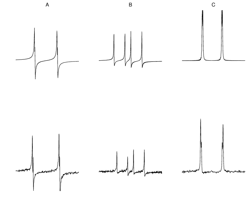
Figure 1 shows selected theoretical and experimental spectra following the quantum Fourier transform of the state on the three qubit NMR quantum computer.
The fidelity of the QFT calculated using the measure
| (38) |
is 87%. Here is the density matrix minus the part that is proportional to the identity (in NMR, this is called the ‘reduced’ density matrix; it should not be confused with the reduced density matrix got by partially tracing the density matrix for a composite quantum system over some of its subsystems). This measure reflects both imperfections in the applied pulses and delays, as well as decoherence. To a first approximation, decoherence during the course of the QFT attenuates the entire density matrix. This is shown in figure 2. Therefore, we can approximately separate the errors caused by experimental imperfections by renormalizing to its attenuated average. Using this the fidelity of the operations themselves is above 98% over the 6 gates in (11).
The fidelity of 87% corresponds to an error rate of 97.7% over the six gates which, while high, does not attain the error rate of required for robust quantum computation [22]. These errors arise primarily from spatial inhomogeneities in the radio frequency fields which we believe can be improved.
In conclusion, using NMR, the QFT has been implemented on a three bit quantum system and the fidelity with which we can transform an initially diagonal state has been measured. Although the fidelity does not reach that required for fault tolerant computing, it is easily high enough to permit studies on small quantum systems including quantum simulations. A particularly straightforward use of the QFT is in quantum chaos: as Balazs and Voros [23] pointed out, a simple version of the quantum baker’s map can be performed by QFTs and Schack [24] has shown how such a quantum map might be realized on a quantum computer [25].
The authors thank S. S. Somaroo and C. H. Tseng for helpful discussions. This work was supported by DARPA.

References
- [1] P. W. Shor, Polynomial-Time Algorithms for Prime Factorization and Discrete Logarithms on a Quantum Computer, Siam. J. Comput. 26 1484-1509 (1997), quant-ph/9508027.
- [2] L. Grover, Proceedings, 28th Annual ACM Symposium on the Theory of Computing (STOC), May 1996, pages 212-219.
- [3] S. Lloyd, Universal Quantum Simulators, Science, 273, 23 Aug. 1996.
- [4] P. Benioff, J. Stat. Phys. 22, 563, 1980.
- [5] R. P. Feynman, Simulating Physics with Computers, International Journal of Theoretical Physics, 21, Nos. 6/7, 1982.
- [6] D. Deutsch, Quantum theory, the Church-Turing principle and the universal quantum computer, Proc. R. Soc. Lond. A 400, 97-117 (1985).
- [7] A. Steane, Rept. Prog. Phys. 61, 117-173 (1998).
- [8] D. P. DiVincenzo, Two-Bit Gates are Universal for Quantum Computation, Phys. Rev. A 51, 1015 (1995).
- [9]
For an in depth discussion of quantum computing see lecture notes of J. Preskill http://www.caltech.edu/subpages/pmares.
html. - [10] D. S. Abrams, and S. Lloyd, Simulations of many-body Fermi systems on a universal quantum computer, Phys. Rev. Lett. 79 (1997).
- [11] S. S. Somaroo, et al, Quantum Simulations on a Quantum Computer, quant-ph/9905045.
- [12] D. S. Abrams and S. Lloyd, A quantum algorithm providing exponential speed increase for finding eigenvalues and eigenvectors, quant-ph/9807070.
- [13] C. Zalka, Efficient Simulation of Quantum Systems by Quantum Computers Proc. Roy. Soc. Lond. A 454 (1998) 313-322.
- [14] S. Wiesner, Simulations of Many-Body Quantum Systems by a Quantum Computer, quant-ph/9603028.
- [15] D. Coppersmith, An Approximate Fourier Transform Useful in Quantum Factoring, IBM Research Report RC19642, 1994.
- [16] A. Ekert and R. Jozsa, Quantum Computation and Shor’s Factoring Algorithm, Rev. Mod. Phys., 68, No. 3, 1996.
- [17] R. Jozsa, Quantum Algorithms and the Fourier Transform, Proc. Roy. Soc. Lond. 454 (1998).
- [18] S. Lloyd, Science, 261, 1569-1571, 1993.
- [19] D. G. Cory, A. F. Fahmy, and T. F. Havel, Proc. Nat. Acad. Sci. 94, 1634.
- [20] N. A. Gershenfeld and I. L. Chuang, Bulk Spin-Resonance Quantum Computation, Science, 275, 17 Jan. 1997.
- [21] S. S. Somaroo, D. G. Cory, T. F. Havel, Expressing the operations of quantum computing in multiparticle geometric algebra, Phys. Lett. A, 240, 1998.
- [22] E. Knill, R. Laflamme, W. H. Zurek, Resilient Quantum Computation: Error Models and Thresholds, Proc. Roy. Soc. Lond. 454 (1998).
- [23] N. L. Balazs and A. Voros, The Quantized Baker’s Transformation, Ann. of Phys., 190, (1989).
- [24] R. Schack, Using a Quantum Computer to Investigate Quantum Chaos, Phys. Rev. A 57 (1998).
- [25] This can also help study decoherence see W. H. Zurek and J. P. Paz, Quantum Chaos: A Decoherent Definition, Physica D 83 (1995).