1.4
Random Hamiltonian Models and Quantum Prediction Algorithms
Abstract
This paper describes an algorithm for selecting a consistent set within the consistent histories approach to quantum mechanics and investigates its properties. The algorithm select from among the consistent sets formed by projections defined by the Schmidt decomposition by making projections at the earliest possible time. The algorithm unconditionally predicts the possible events in closed quantum systems and ascribes probabilities to these events. A simple random Hamiltonian model is described and the results of applying the algorithm to this model using computer programs are discussed and compared with approximate analytic calculations.
1 Introduction
It is hard to find an entirely satisfactory interpretation of the quantum theory of closed systems, since quantum theory does not distinguish physically interesting time-ordered sequences of operators. In this paper, we consider one particular line of attack on this problem: the attempt to select consistent sets by using the Schmidt decomposition together with criteria intrinsic to the consistent histories formalism. For a discussion of why we believe consistent histories to be incomplete without a set selection algorithm see [1, 2] and for other ideas for set selection algorithms see [3, 4, 5, 6]. This issue is controversial: others believe that the consistent histories approach is complete in itself [7, 8, 9].
1.1 Consistent histories formalism
We use a version of the consistent histories formalism in which the initial conditions are defined by a pure state, the histories are branch-dependent and consistency is defined by Gell-Mann and Hartle’s medium consistency criterion eq. (3). We restrict ourselves to closed quantum systems with a Hilbert space in which we fix a split ; we write and we suppose that . The model described in sec. 2 has a natural choice for the split. Other possibilities are discussed in [3].
Let be the initial state of a quantum system. A branch-dependent set of histories is a set of products of projection operators indexed by the variables and corresponding time coordinates , where the ranges of the and the projections they define depend on the values of , and the histories take the form:
| (1) |
Here, for fixed values of , the define a projective decomposition of the identity indexed by , so that and
| (2) |
Here and later, though we use the compact notation to refer to a history, we intend the individual projection operators and their associated times to define the history.
We use the consistency criterion11 1 For a discussion of other consistency criteria see, for example, refs. [10, 11, 12, 13].
| (3) |
which Gell-Mann and Hartle call medium consistency, where is the decoherence matrix
| (4) |
Probabilities for consistent histories are defined by the formula
| (5) |
With respect to the splitting of the Hilbert space, the Schmidt decomposition of is an expression of the form
| (6) |
where the Schmidt states and form, respectively, an orthonormal basis of and part of an orthonormal basis of , the functions are real and positive, and we take the positive square root. For fixed time , any decomposition of the form eq. (6) then has the same list of probability weights , and the decomposition (6) is unique if these weights are all different. These probability weights are the eigenvalues of the reduced density matrix.
The idea motivating this paper is that the combination of the ideas of the consistent histories formalism and the Schmidt decomposition might allow us to define a mathematically precise and physically interesting description of the quantum theory of a closed system. We consider constructing histories from the projection operators22 2 There are other ways of constructing projections from the Schmidt decomposition [3], though for the model considered in this paper the choices are equivalent.
| (7) |
which we refer to as Schmidt projections. If the complementary projection is zero. In developing the ideas of this paper, we were influenced in particular by Albrecht’s investigations [14, 15] of the behaviour of the Schmidt decomposition in random Hamiltonian interaction models and the description of these models by consistent histories.
2 A Random Hamiltonian Model
Consider a simple quantum system consisting of a finite Hilbert space (), a pure initial state and a Hamiltonian drawn from the GUE (Gaussian Unitary Ensemble), which is defined by
| (8) |
where is a normalisation constant.
The GUE is the unique ensemble of Hermitian matrices invariant under with independently distributed matrix elements, where . The GUE is also the unique ensemble with maximum entropy, , subject to and . The book by Mehta [16] contains a short proof of this as well as further analysis of the GUE and related ensembles. All the results concerning the GUE in this thesis can be found in this book or in the appendix.
This model is not meant to represent any particular physical system, though Hamiltonians of this from are used in models of nuclear structure and have often been studied in their own right (see [16, 17] and references therein), and a large class of other ensembles approximate the GUE in the large limit.
Because is drawn from a distribution invariant under there is no preferred basis, no distinction between system and environment degrees of freedom and no time asymmetry. In other words the model is chosen so that there is no obvious consistent set: we do not already know what the answer should be. Moreover it does not single out a pointer basis that one might associate with classical states, so that the Copenhagen interpretation cannot make any predictions about a model like this in the limit. If an algorithm works for this model, when there are no special symmetries, it should work for a wide variety of models. The question whether a pointer basis can arise dynamically using Schmidt states was addressed by Albrecht in [14, 15], but no general prescription emerged from his study. Albrecht also studied the relationship between Schmidt states and consistent histories, and his studies suggested that the relationship was complicated.
The model considered here generalises Albrecht’s model: the Hamiltonian for the entire Hilbert space is chosen from a random ensemble. Albrecht also used a different distribution, but as we explain below the GUE seems more natural, though this it probably makes little difference.
Without loss of generality, we take and . With this choice and using the Hermiticity property of eq. (8) becomes
| (9) |
Therefore the diagonal elements are independently distributed, real normal random variables with mean and variance and the off-diagonal elements are independently distributed, complex normal random variables with mean and variance .
Since the Hamiltonian is invariant under the only significant degrees of freedom in the choice of initial state are the initial Schmidt eigenvalues (the eigenvalues of the initial reduced density matrix.) The usual choice in an experimental situation is an initial state of the form which corresponds to a pure initial density matrix. A more general choice in the spirit of the model is to draw the initial state from the invariant distribution subject to fixed rank . This is equivalent to choosing the first eigenvalues to be components of a random unit vector in and the remaining components to be zero.
3 Analysis
The calculations in this section are an attempt to gain insight into the expected properties of prediction algorithms applied to the random model. These calculations rest on a large number of assumptions and are at best approximations, but the conclusions are borne out by numerical simulations and the calculations do provide a rough feel for the results that different algorithms can be expected to produce. In particular they suggest that there are only narrow ranges of values for the approximate consistency parameter which are likely to produce physically plausible sets of histories. These calculations may also be applicable to other models since this model makes so few assumptions and the interaction is completely general.
In a random model there is no reason to expect exactly consistent sets of histories formed from Schmidt projections to exist, so only parameterised approximate consistency criteria such as the frequently used criterion [18, 19]
| (10) |
or the DHC (Dowker-Halliwell Criterion) [12, 13]
| (11) |
or
| (12) |
are considered in this paper and will always be the consistency parameter in these equations. We shall only discuss medium consistency criteria: the results for weak consistency are qualitatively the same.
Approximate consistency criteria were analysed further in ref. [13]. As refs. [12, 13] explain, the DHC has natural physical properties and is well adapted for mathematical analyses of consistency. We adopt it here, and refer to the largest term,
| (13) |
of a (possibly incomplete) set of histories as the Dowker-Halliwell parameter, or DHP.
If an absolute approximate consistency criterion is being used there are strong theoretical reasons for imposing a parameterised non-triviality criterion [13]. However, if the approximate DHC is being used one is not needed, though it is convenient to introduce one for computational reasons. The non-triviality parameter (which we shall always write as in this chapter) can be taken very small if the DHC is used and is not expected to influence the results — except possibly for the first projections — and the numerical simulations show that this is indeed the case. We shall refer to histories with probability less than or equal to (relative or absolute) as trivial histories and a projection that gives rise to a trivial history as a trivial projection. There are no absolute reasons for rejecting set of histories containing trivial histories — if is sufficiently small and there are not too many they are physically irrelevant — though obviously sets are preferable if all the histories are non-trivial. However, an algorithm must produce results that are approximately the same for a range of parameter values if it is to make useful predictions, and trivial histories will almost certainly vary as is changed. If the DHC is used, generically all the later projections will also change, since trivial histories can significantly influence the consistency of later projections. If an absolute consistency criterion is used trivial projections are more likely to be consistent than non-trivial projections so for many values of the parameters only trivial will be projections are made.
3.1 Repeated projections and relative consistency
Consider a history extended by the projective decomposition and the further extension of history by . This was discussed for the DHC in refs. [13, 3] and the DHP for this case was shown to be
| (14) |
The reprojection will occur unless , the approximate consistency parameter, is smaller than (14). It is easy to show that the time evolution of Heisenberg picture Schmidt projections is
| (15) |
where is the Hamiltonian,
| (16) |
are projection operators (in ) on to the Schmidt eigenspaces, their respective (distinct) eigenvalues and the derivative of the reduced density matrix.
In analysing (14) and similar expressions we make the following assumptions. First that is uncorrelated with the Schmidt states — this generally is a good approximation when there are a large number of histories. Second that is an operator drawn from the GUE with unspecified variance independent of the other variables — in some situations this assumption is exact but it generically is not.
Let , an element of the GUE with variance , then using eq. (15) (14) is
| (17) |
Because is drawn from a distribution invariant under and is independent of and , (17) can be simplified by choosing a basis in which and . (17) becomes
| (18) |
where and . Since is a set of independent, complex, normal random variables, (18) is the square root of a random variable33 3 :- a beta random variable with parameters and . This has a density function . A B(1,r-1) random variable has the same distribution as that of the inner-product squared between two independent unit vectors in ..
Suppose we choose so that reprojections will occur with some small probability — note that only choosing will definitely prevent all repeated projections. The probability of (18) being less than is
| (19) |
Therefore if
| (20) | |||||
a reprojection will occur with probability .
However, it is shown in [3] that the DHC cannot prevent trivial reprojections on the initial state if the initial density matrix has less than full rank. If the initial density matrix has rank one then the first projection will always be made with probability . A non-triviality criterion can then work in conjunction with the DHC to prevent further trivial extensions. Suppose either that the initial density matrix has rank greater than and and are two projections onto the non-zero eigenspaces, or assume that the rank is one and is a projection onto the initial state and is a projection making a history of probability . In either case, let be projection onto the null space. To prevent the trivial projection being made the parameters and must be chosen to satisfy [3]
| (21) |
Though the probability distribution for this is complicated, the approximate relation between and can be estimated by squaring both sides of eq. (21) and then taking the expectation. Note that treating as an element of the GUE is exact in this case as the terms involving are identically zero. Using results from eq. (36), eq. (21) becomes
| (22) |
where is the rank of . By assumption is order one and , so if initial reprojections will not occur. The results are the same for a relative non-triviality criterion since instead of eq. (22) we have .
3.2 Repeated projections and absolute consistency
An algorithm using an absolute parameterised consistency criterion will make nothing but trivial projections unless a parameterised non-triviality criterion is also used, so only algorithms with a non-triviality criterion are considered.
Let denote the latest time that the reprojection is approximately consistent and the earliest time at which the extension is absolutely nontrivial. We see from refs. [13, 3] that, to lowest order in ,
| (23) | |||||
| (24) |
implies
| (25) |
Again we choose so that reprojections occur with probability q and assume that and are order one, so that eq. (25) can be written
| (26) |
The l.h.s. is the same random variable as in eq. (18) so and must be chosen so that
| (27) |
The assumption that and are order one will obviously not always be valid. As more projections are made the probabilities of the histories will decrease. When both probabilities are eq. (25) is
| (28) |
so . If reprojections of smaller probability histories are to be prevented this choice of parameters is clearly more appropriate than eq. (27).
This analysis has picked a very conservative upper bound for to prevent repeated projections, since decoherence matrix terms with the other histories will tend to reduce the likelihood of repeated projections, and thus allow larger values of to be used. A more detailed analysis suggests that for relative and absolute consistency can be treated as much smaller than so that choosing a small factor larger than or respectively, are sufficient conditions.
3.3 Projections in the long time limit
The previous subsection has shown how and affect the probability of repeated projections: this subsection calculates how they affect the probability of projections as . In infinite dimensional systems, off-diagonal terms of the decoherence matrix for quasiclassical projections often tend to zero as increases [20]. In the limit one would also expect this for Schmidt projections in this model — though the limit only exists for initial density matrices of finite rank.
Consider the DHP for a Schmidt projection extending history from the set of normalised exactly consistent histories as . For and for large the Schmidt states are approximately uncorrelated with the histories. The DHP for an extension of history is
| (29) |
Since for all , eq. (29) is equal to (within a factor of )
| (30) |
The cumulative frequency distribution for (30) squared is calculated in [4] as
| (31) |
which approximately equals when . This is the probability that a pair of projections acting on one history in a set of consistent histories satisfies the medium DHC with parameter . There are distinct choices for the projections so the DHP (to within a factor of ) for extending with any Schmidt projection is
| (32) |
where range over all binary partitions of the basis Schmidt projections. The distribution for this random variable is hard to calculate but if we assume that the DHP’s for each are independent the cumulative distribution function is
| (33) |
This assumption is obviously very approximate since the different projections are all formed using the same basis. However, treating the as independent in (32) will be a lower bound for the exact result and (30) will be an upper bound for the exact result.
Suppose now we wish to choose so that the probability of making a projection at a large time is , where is close to one. Then from eq. (33)
| (34) |
For large
| (35) |
This calculation has involved a lot of assumptions and approximations, but it should accurately reflect the behaviour for . The logarithmic dependence on is a generic feature of extreme order statistics and so is the independence of the answer from the other factors and . The dependence is also expected because the mean value of the square of the inner product between two random vectors in a dimensional space is .
A generic feature of asymptotic extreme order statistics such as the previous calculation, is the slow rate of convergence and this calculation is only expected to be accurate for very large and . For actual application to particular models the exact distribution can be calculated by a computer program using Monte-Carlo methods.
For each sample the program randomly picks a set of exactly consistent histories, and then calculates the DHP for all combinations of projections on one particular history. Ten thousand samples were sufficient to produce smooth cumulative frequency distributions. These can be inverted to calculate as in fig. (1), where for example is the solid curve.
The same arguments apply for absolute consistency as , but since the consistency requirement is not normalised the expected DHP values will be reduced by a factor of — the average value for the length of a history when there are histories.
These calculations suggest that choosing is most likely to produce histories with a complicated branching structure and many non-trivial projections. In the next section we discuss the results of simulations for all values of the parameters and show that they agree with these theoretical calculations.
4 Computer simulations
The computer programs are explained and listed in ref. [4]. The results described here were carried out with a system of dimension , with an environment of dimension and with either medium absolute consistency or medium relative consistency (DHC). Fig. (1) gives the probability distribution for the DHP plotted via percentile curves as a function of the number of histories in the long time limit. For example, this graph shows that with projections will almost certainly be consistent for any number of histories, whereas for projections will probably only be consistent when there are two or three histories. When there are twenty histories it shows that for of the time the DHP will be between and . Fluctuations will only occasionally ( of the time) lie below the solid line and if has this value (for a particular number of histories) then although projections will probably occur they will occur as a result of large fluctuations from the mean. Therefore one would expect the projections to occur at widely separated times and if is changed only slightly the times generically to change completely, and indeed computer simulations show this.

The simulations described here were run for ten thousand program steps or until thirty histories had been generated. For a given set of parameters, many simulations with different Hamiltonians and initial states were carried out and were found generically to produce qualitatively the same results, though only individual simulations are described here.
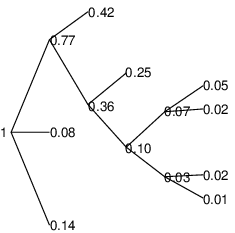

One way to look at the results of a simulation is to look at the probability tree associated with the set of histories such as fig. (2a). The root node on the far left represent the initial state, the terminal nodes represent the histories and the other nodes represent intermediate path-projected states. Each node has a probability and the lines linking the nodes have an associated projection operator and projection time. The projections associated with lines emanating to the right from the same node form a projective decomposition and all occur at the same time. The scaling of the axis and relative positions between the nodes is arbitrary, only the topology is relevant. For example, in fig. (2a) the probabilities for the histories are , , , , , , and — the probabilities of the terminal nodes.
Another useful interpretative aid is a graph of the consistency statistics fig. (2b). This graph shows the DHP for the most consistent non-trivial extension. At times where no Schmidt projections result in non-trivial histories no points are plotted, though there are no such times in fig. (2b). The program makes a projection when this value is . The flat line indicates and the crosses indicate when projections have occurred — in this case at times , , , , and (approximately). A graph of the projection times will also be used sometimes, for example fig. (4b).
When any Schmidt eigenvalues are equal their eigenspaces becomes degenerate and the corresponding Schmidt projections are not uniquely defined. The reduced density matrix varies continuously in this model and it will only be degenerate for a set of times of measure zero so generically it is possible to define the Schmidt states so that they are continuous functions of for all . This was not found to be necessary in the simulations.
4.1 Results for relative consistency
4.1.1 Rank one initial density matrix


Fig. (3) shows the probability tree and minimum consistency statistics for a simulation with and a rank one initial density matrix. As expected there is one almost immediate trivial projection. Three more projections occur and then no more. From fig. (1) the probability of a projection with five histories and is less than 1% so this result is as expected. The simulation was run for longer than is shown in the figure (until ) but no further projections occurred.


Fig. (4) shows the probability tree and projection times for a simulation with . Again there is the initial trivial projection but no other trivial projections occur. Projections then occurred at roughly equal equal time intervals until there were fifteen histories. The time between projections then rapidly increased. This is in accord with fig. (1) as the probability for a projection with fifteen histories and is around . Projections after this time only occur for large deviation away from the mean and therefore occur extremely erratically. These later projections are extremely unlikely to vary smoothly for a range of . The simulation was run until and no further projections occurred. This simulation has produced an interesting set of histories with a complicated branching structure.
The next pair of figures fig. (5) shows the results of a simulation with all the parameters unchanged except for which is now . The qualitative description is the same and the first eight or so projections are similar. After that however the two sets of histories are very different. This is the problem with the algorithm applied to this model: interesting sets of histories are produced, but they change dramatically for small changes in .
From fig. (1) choosing looks large enough so that projections will always be made before the background level is reached. The theoretical analysis also suggests that for such a large value of some repeated projections will occur. Indeed fig. (6) demonstrates that nine repeated projections occurred each giving a history of probability .


consistency statistics
An interesting alternative is to choose as a percentile from fig. (1), that is where is the number of histories. Fig. (7) demonstrates the consistency statistics for a run with chosen at the level. All of the probabilities except for the initial projection were non-trivial. Rather than the projections being made in regimes where the DHP fluctuates about its mean value most of the projections have been made at times when the DHP is monotonically decreasing, so that the histories are much more likely to vary continuously with . Two other advantages of choosing this way are that larger sets of histories are produced, and if an algorithm is designed to produce a set of histories of a certain size choosing in this way will produce a more consistent set than choosing to be constant. However, though the results are more stable (when the percentile is changed) than for constant , results from simulations show that they still change too much to single out a definite set of histories.
By looking at the consistency statistics the problem is easy to understand. Since a projection is made at the earliest possible time generically once it has been made the DHP jumps up as the most consistent projection has occurred. The consistency level then falls. While it is decreasing monotonically any change in will produce a continuous change in the time of the next projection. However, if is too far below its mean level the projection times will vary discontinuously, and all the projections afterwards will generically be completely different. Since the mean level of the DHP depends on the number of histories strongly either must be chosen sufficiently large so as to be above this or it must be chosen so as to increase with the number of histories. This is demonstrated by the first few projections as shown in fig. (8) — a close-up of fig. (7b) would also show this.
4.1.2 Other initial conditions


Simulations with a rank 2 initial state, and all other parameters remaining the same, produce the same results except that each of the initial projections is repeated producing two trivial histories with probability . We can choose according to eq. (22) to try to prevent these projections, that is choose . Since many of the histories we expect to generate will have probabilities smaller than this it is sensible to use a relative non-triviality criterion44 4 Using a relative non-triviality criterion earlier does not qualitatively change the results except that the initial trivial history would also have been extended — the results would have been qualitatively the same as for rank two initial reduced density matrices.. The analysis leading to eq. (22) is only accurate to first order in , therefor eq. (22) is only valid when is sufficiently small. If is too large the consistency level of a reprojection will start decreasing and when a reprojection eventually becomes non-trivial it will be consistent. For the example discussed there were no values of with that prevent an initial trivial reprojection. Fig. (8) demonstrates the start of a simulation with and . The graph of the consistency statistics shows the initial projection at and then that there are no non-trivial extensions until by which time the projection is not consistent. A non-trivial projection is made at and the algorithm then continues as before, with the trivial projection avoided. Because the projection has not occurred with probability there is a range of values for that do not affect the resulting histories — they are independent of . The first three projection times will obviously vary continuously for a small range of . The other projections that occurred in this simulation all occurred at much more separated times in a regime where the consistency level was not decreasing monotonically. If is chosen according to the percentile distribution in fig. (1) — that is where is the number of histories — will be small enough initially to prevent any trivial projections (with an initial density matrix of rank greater than one) and will allow a full set of histories to be built up at later times.
Simulations with a full rank initial density matrix and result in a trivial repeated projection for each initial history. If is smaller () no trivial reprojections occur. If two initial projections are made uncorrelated with the Schmidt states then further (Schmidt) projections at will not generically be trivial or consistent. In both cases, after the initial projections and possible reprojections the qualitative behaviour is the same as the rank one case.
4.2 Results for absolute consistency
To produce interesting sets of histories from an absolute consistency criterion three effects need to be balanced against each other. If is too small the most likely projections will be those that produce very small probability histories. If is too small the likelihood of repeated projections (hence trivial histories) will be high. If is too large the non-triviality criterion will dominate the algorithm and only probability (trivial) histories will be produced. Only an absolute parameterised non-triviality criterion is considered since a relative criterion will clearly produce almost nothing except infinitesimal histories. The following results demonstrate these effects.
4.2.1 Rank one initial density matrix

For example if and the initial reduced density matrix has rank one the algorithm will generically produce trivial histories. This is a particularly simple case of the analysis that suggests that if repeated projections are probable. Fig. (9) shows an example of this from a computer simulation with and . Only the first ten projections are shown. This behaviour remains the same in the limit as .

probability tree
As the ratio increases and becomes the nature of the set of histories changes. Occasionally when a reprojection becomes non-trivial it will no longer be consistent and a reprojection will not occur. A significant time may elapse before the next projection is made which will result in a non-trivial projection, which will then be followed by more trivial repeated projections. This is demonstrated in fig. (10) where and . Though this is an interesting set of histories this range of parameter values does not give a theory with predictive power since simulations show that the results vary enormously for small changes in and .


As increases past the number of histories made with probability decreases to just the initial projection. Fig. (11) shows that this range of parameter values produces interesting histories but the projections are occuring at times when the consistency level is fluctuating randomly about the mean and so will be unstable to small changes in .
4.2.2 Other initial conditions
Choosing larger rank initial reduced density matrices or initial projections does not qualitatively change the analysis. The only difference is that for and sufficiently small no trivial projections will be made.
5 Conclusions
The algorithm produces sets of histories with a complicated branching structure and with many non-trivial projections for a range of parameter values. Algorithms using the DHC produce results that are essentially the same for a wide range of (the non-triviality parameter) including the limit . However, the algorithm does not make useful predictions when applied to this model since the results vary erratically with and there is no special choice of singled out. Choosing as a function of the number of histories according to fig. (1) produces the least unstable sets of histories and the largest sets of non-trivial histories, but even in this case the algorithm does not single out a definite set.
The algorithm is less effective when used with an absolute consistency criterion: in this case the predictions of the algorithm also vary erratically with and the resulting sets of histories include fewer non-trivial histories.
The results of the simulations agree well with the theoretical analysis of section (3) and demonstrate features of the algorithm that will also apply to other models — such as the analysis of repeated projections. They also demonstrate some of the difficulties that an algorithm must overcome. These problems can be related to the discussion of recoherence in refs. [3]. The algorithm will only produce stable results (with respect to ) if the projections occur when the off-diagonal terms of the decoherence matrix are monotonically decreasing. This behaviour is only likely in a system like this for times small compared to the recurrence time of the system and when the number of histories is small compared to the size of the environment Hilbert space. The results of the model do show stability for the first few projections and if much larger spaces were used this behaviour would be expected for a larger number of histories. In particular as the size of the environment goes to infinity it is plausible that the algorithm applied to this model will produce a large, stable, non-trivial set of histories.
The Gaussian Unitary Ensemble
In the GUE the matrix elements are chosen according to the distribution
where , and . Therfore all the elements are independently, normally distributed, the diagonal with variance and the real and imaginary off-diagonal with variance . Some expectations for a normal variable with variance are
and in particular , and . Since is independent of unless and , or and
Therefore, for the elements of
Applying these results to vectors and projection operators,
| (36) | |||||
where is the rank of . For the real part or the imaginary part just take half of the above since .
References
- [1] F. Dowker and A. Kent, Phys. Rev. Lett. 75, 3038 (1995).
- [2] F. Dowker and A. Kent, J. Stat. Phys. 82, 1575 (1996).
- [3] J. N. McElwaine and A. Kent, Phys. Rev. A 55, 1703 (1997).
- [4] J. N. McElwaine, Ph.D. thesis, DAMTP, Cambridge University, 1996.
- [5] M. Gell-Mann and J. B. Hartle, gr-qc/9509054, University of California, Santa Barbara preprint UCSBTH-95-28.
- [6] C. J. Isham and N. Linden, Phys. Rev. A 55, 4030 (1997).
- [7] R. Omnès, The Interpretation of Quantum Mechanics (Princeton University Press, Princeton, 1994).
- [8] R. B. Griffiths, Phys. Rev. A 54, 2759 (1996).
- [9] M. Gell-Mann and J. B. Hartle, in Complexity, Entropy and the Physics of Information, Vol. III of SFI Studies in the Science of Complexity, edited by W. H. Zurek (Addison Wesley, Reading, 1990).
- [10] A. Kent, gr-qc/9607073, DAMTP/96-74, submitted to Ann. Phys.
- [11] S. Goldstein and D. N. Page, Phys. Rev. Lett. 74, 3715 (1995).
- [12] H. F. Dowker and J. J. Halliwell, Phys. Rev. D 46, 1580 (1992).
- [13] J. N. McElwaine, Phys. Rev. A 53, 2021 (1996).
- [14] A. Albrecht, Phys. Rev. D 46, 5504 (1992).
- [15] A. Albrecht, Phys. Rev. D 48, 3768 (1993).
- [16] M. L. Mehta, Random Matrices, 2nd ed. (Academic Press, London, 1991).
- [17] B. D. Simons and B. L. Altshuler, Phys. Rev. Lett. 70, 4063 (1993).
- [18] M. Gell-Mann and J. B. Hartle, Phys. Rev. D 47, 3345 (1993).
- [19] R. Omnès, Ann. Phys. 201, 354 (1990).
- [20] W. H. Zurek, Phys. Rev. D 26, 1862 (1982).