The problem of equilibration and the computation of correlation functions on a quantum computer
Abstract
We address the question of how a quantum computer can be used to simulate experiments on quantum systems in thermal equilibrium. We present two approaches for the preparation of the equilibrium state on a quantum computer. For both approaches, we show that the output state of the algorithm, after long enough time, is the desired equilibrium. We present a numerical analysis of one of these approaches for small systems. We show how equilibrium (time)-correlation functions can be efficiently estimated on a quantum computer, given a preparation of the equilibrium state. The quantum algorithms that we present are hard to simulate on a classical computer. This indicates that they could provide an exponential speedup over what can be achieved with a classical device.
pacs
PACS numbers: 03.67.Lx, 05.30.-d, 89.80.+h, 02.70.LqI The limits of classical computation
The power of quantum computers has been demonstrated in several algorithms, of which the most striking have been Shor’s factoring algorithm [1, 2] and Grover’s search algorithm [3]. From the very start however, the quantum computer has also held the promise of being a simulator of physical systems. This is the content of the physical version of the Church-Turing principle proposed by Deutsch [4]. Thus we might expect that the universal quantum computer can be used to simulate any experiment that we could do on a real physical system. If such a simulation can be done efficiently (that is, without exponential slowdown), it is clear that this could be one of the major applications of a quantum computer. This promise seems to have been only partly fulfilled until now; it has been shown by several researchers [5, 6] that a simulation of the unitary time evolution of a physical system that possesses some degree of locality (which realistic physical systems do) can be accomplished efficiently on a quantum computer. However, many quantities of interest that are determined by experiment, or by the use of classical simulation techniques, relate to open quantum systems, in particular to systems in thermal equilibrium. The thermal equilibrium (Gibbs) state (in the canonical ensemble) of a Hamiltonian is given by
| (1) |
where () are the eigenvectors (eigenvalues) of . is the partition function
| (2) |
and where is Boltzmann’s constant and the temperature. The physical systems that concern us in this paper will have a finite dimensional Hilbert space that can be decomposed as
| (3) |
where each represents a small, constant Hilbert space, typically associated with some (generalized) spin or other local degree of freedom. The Hamiltonian couples these local Hilbert spaces, for example in correspondence with a -dimensional spatial lattice, so that there is only coupling between adjacent “spins” on this lattice. The quantities of interest, computed in experiment or in a classical computation, are of the form
| (4) |
where are (possibly time-dependent) observables. Both for classical systems as well as for quantum systems, computational Monte Carlo methods have been developed to estimate correlation functions as in Eq. (4) [7, 8, 9]. The quantum Monte Carlo method for systems at finite temperature relies on a transformation introduced by Suzuki [10] that maps an initial quantum system on a -dimensional lattice onto a -dimensional classsical system. This conversion then makes it possible to use classical computational sampling techniques to estimate correlation functions as in Eq. (4). There seem to be (at least) two situations when this approach runs into trouble and no good computational alternatives are available [9]: (1) the correlation functions depend explicitly on time , and (2) the quantum system is of a fermionic nature. We will give a short explanation of why these problems are encountered.
The transformation from a classical to a quantum system is based on the generalized Trotter formula. Let where each is a Hamiltonian on a small constant Hilbert space. The Trotter formula reads
| (5) |
The partition function Eq. (2) (and similarly correlation functions as in Eq. (4)) can be rewritten, using the Trotter formula and the identity , where the pair of indices labels a choice of basis, as
| (6) |
where is a distribution over the values of the collection of variables and indexes the repetitions of the factors of Eq. (5) from 1 to . If the distribution is nonnegative, we can write where is now a classical Hamiltonian given by
| (7) |
with , and
| (8) |
The distribution will only be nonnegative when the matrix elements are positive. Thus it is important to choose the right sets of basis states to make the conversion to a classical sampling problem with a positive distribution. There are fermionic systems such as certain Hubbard models [9] in which it does not seem to be possible to choose such a good basis. For these systems it has turned out to be very hard to get good estimates of correlation functions by using classical Monte Carlo techniques. This problem is usually referred to as the “sign” problem.
When we are to compute time-dependent quantities, for example the function , we need to use an imaginary time to perform the conversion of Eq. (5) to a classical system (we expand with the Trotter formula). From the classical Monte Carlo sampling of the function for real , we estimate and then we could in principle analytically continue this function. However, we only have a finite number of samples of the function and each sample point has some inaccuracy. The errors that are introduced in estimating the Fourier components from this data give rise to large fluctuations when we reconstruct with the Laplace transform
| (9) |
resulting in a bad approximation for the time correlation function .
The relevance of estimating a simple time correlation function (an example of Eq.(4)) such as
| (10) |
where and are some Hermitian Heisenberg operators of the system, cannot be overestimated. Let us recall the many contexts in which Eq.(10) is used in describing experimental properties of many-particle quantum systems [11]:
When , where is the displacement field of a crystal, (10) describes the phonon dynamics of solids as probed by inelastic neutron scattering. When and are the number-density operator, the dielectric susceptibility is represented; this correlation function describes a variety of other experiments, including x-ray photoemission and the so-called x-ray edge singularity. When we study the current-current response function, we obtain the electrical conductivity as described by the Kubo formula. (The density-density and current-current response functions are intimately related via the continuity equation.) Spin-dependent quantities are also of interest: with the spin-spin correlation function, information is obtained about the magnetic susceptibility, and thus the magnon dynamics of ferromagnets and antiferromagnets, the Kondo effect, and the magnetic-dipole channel in neutron scattering. And finally, if and involve anomalous pair amplitudes which involve Fermion operators like , the presence and dynamics of a superconducting phase can be probed.
In short, the dynamic pair correlation functions provide a window on many of the interesting quantities in experimental physics, and it would be highly desirable to have a method of obtaining estimates for these quantities by simulation on a quantum computer. We will present some methods below for doing this.
In this paper we develop an approach to tackle these problems on a quantum computer. We break the problem into two parts: First, we present an approach to prepare our quantum computer in the equilibrium state of a given Hamiltonian (sections II and III). We will give two alternative routes to prepare an equilibrium state. Next we describe a procedure for efficiently estimating quantities as in Eq. (4) given that the equilibrium state has been prepared (section IV). We will not attempt to prove that our algorithms run in polynomial time even for a certain class of quantum systems and/or for certain ranges of . The equilibration problem, in its full generality, is expected to be a hard problem. Even classically there is a large class of systems that exhibit a feature called frustration, for which calculating the partition function as in Eq. (2) is a -complete problem [12]. Also, for these systems, deciding whether the energy of the ground state is lower than some constant is an NP-complete problem [13]. The quantum problem has an added difficulty: We cannot assume that we know the eigenvectors (and eigenvalues) of the Hamiltonian of the system that we would like to equilibrate. There has been no demonstration yet that a quantum computer can exponentially outperform a classical computer in estimating the partition function for certain classical systems, which would enable us to sample efficiently from the classical Gibbs distribution [14].
The quantum algorithms that we present are hard to simulate on a classical computer. In both of our equilibration algorithms we use the fact that one can implement the unitary time evolution of a local Hamiltonian on qubits in a polynomial number of steps in on a quantum computer [5]. A direct simulation of this procedure on a classical computer would cost exponential (in ) space and time and is therefore unrealistic. As we will show in section IV, given a preparation of an equilibrium state, there exists an efficient procedure on a quantum computer to calculate (time-dependent) correlation functions. As we discussed above, there is no general efficient classical algorithm with which one can estimate time-dependent correlation functions. Our quantum algorithm provides such an algorithm for a quantum computer. Lloyd and Abrams [16] have shown that the unitary simulation of a fermionic system such as the Hubbard model, either in first or second quantization, can be performed efficiently on a quantum computer. The quantum algorithms that we will present will use this unitary evolution as a building block. Therefore these algorithms can be used to compute correlation functions for the Hubbard model on a quantum computer. This is a task for which we do not have a good classical algorithm, due to the “sign” problem, as we pointed out above.
We focus our efforts on quantum equilibration algorithms for Hamiltonians of which the eigenvalues and eigenvectors are not known beforehand. These are the Hamiltonians of, for example, Heisenberg models (in more than two dimensions), Hubbard models, t-J models, XY models, or many-electron Hamiltonians in quantum chemistry. On the other hand, knowing the eigenvectors and eigenvalues of a Hamiltonian, such as in the Ising model, is no guarantee that there exists an efficient (polynomial time) classical algorithm that produces the equilibrium distribution. The situation is similar for quantum algorithms; we do not know in what cases the equilibration algorithms presented in section II and III give rise to a polynomial time algorithm (see also [15] for quantum algorithms for Ising-type models).
The process of equilibration is also essential in the actual realization of a quantum computer. One of the assumptions underlying the construction of a quantum computer [17] is the ability to put a physical system initially into a known state (or a thermal equilibrium state in the NMR quantum computer [18]), the computational state. The way this is done in an experimental setup is to let this state be the ground state of a natural Hamiltonian and subsequently to cool to low temperature such that the probability of being in this ground state is some constant. This natural Hamiltonian must be sufficiently simple for this equilibration to be achievable efficiently and also be sufficiently weak or tunable not to disturb the computation later on.
II Equilibration I
II.1 Introduction
The canonical ensemble is the ensemble of states , or a density matrix , such that has a given energy-expectation value
| (11) |
The equilibrium state in this ensemble (Eq.(1)) can be obtained by maximizing the von Neumann entropy of under this energy constraint. Another way in which the canonical ensemble is defined is by considering the possible states of a system that is in contact with an infinite heat bath at a certain temperature . The total energy of system and bath is constant, but bath and system exchange energy, so that the system equilibrates. This directly suggests that the way to prepare the equilibrium state on a quantum computer is to mimic this process. In considering the computational complexity of such a procedure, we will have to include the space and time cost of the bath, which may be large. Also, the intuitive picture of equilibration between a weakly coupled large bath and system does not tell us anything about the rate at which this equilibration occurs. Furthermore, the equilibration process assumes a bath that is already in its equilibrium state. Can we make the bath simple enough that this bath state can be prepared efficiently? In this section we study this process of equilibration. We present an algorithm and we derive expressions that completely characterize the equilibration process in an idealized case: the coupling between the bath and the system is very small, the bath is very large, and the time of interaction is large. We then proceed by a numerical study of the algorithm in realistic cases where the bath is of finite dimension, the strength of the interaction is non-zero, and the interaction time is limited.
II.2 The algorithm
Definition 1
Equilibration algorithm I.
Input-parameters:
-, the Hamiltonian of a -dimensional quantum system.
- , the inverse temperature.
-, the Hamiltonian of a -dimensional
“bath” quantum system.
-, where is the -dimensional “bath-system”
interaction Hamiltonian and is the parameter that measures the strength of the interaction between bath and system.
-, the interaction time between bath and system.
-, the number of times the bath is refreshed in the algorithm.
Define the total Hamiltonian of system and bath as
| (12) |
and the trace-preserving completely positive () map as
| (13) |
- 1.
Prepare system. We prepare the qubits in the computational state: .
- 2.
Prepare bath. We prepare the qubits of the bath in their equilibrium state of .
- 3.
Evolve system and bath for time and discard bath, that is, perform the superoperator of Eq. (13).
- 4.
Repeat steps 2 and 3 times such that
(14) for all and is some accuracy. See Appendix A for the definition of .
We put several constraints on , and . We will use local Hilbert spaces as in Eq. (3) of dimension 2 (qubits). must be a “local” Hamiltonian. We define a -local Hamiltonian on qubits as one that can be expressed as
| (15) |
where each operates on a tensor product of several small qubit Hilbert spaces, whose total dimension is . We will also assume that the eigenvalues of are all distinct; the spectrum is non-degenerate. This will simplify the upcoming analysis. In order to treat Hamiltonians with degenerate spectra a change in the perturbation theory of Section II.4 will have to be made. We expect however that with that change the main result of Section II.5, namely succesful equilibration in the idealized case, will still hold. has the linear coupling form
| (16) |
where both and are local Hamiltonians. is the Hamiltonian of a system of non-interacting qubits, i.e., it is a sum of single-qubit Hamiltonians:
| (17) |
The bath’s equilibrium state factorizes into a tensor product of qubit equilibrium states associated with each :
| (18) |
This enables us to prepare the bath (step ) efficiently. Appendix B shows that it will cost elementary qubit operations to perform step . The locality of , and is required in order to be able to simulate the unitary time evolution in time proportional to where is the accuracy with which gates are implemented [5, 19].
We also choose
| (19) |
To understand the effect of a non-zero we rewrite as
| (20) |
where . Thus choosing a non-zero effectively corresponds to a change in the Hamiltonian of the system. We now discuss the last step of the algorithm, step 4. When the superoperator has the equilibrium state as its unique fixed point, then Eq. (14) for all implies that that
| (21) |
for all , that is, the equilibration process leads to succesful convergence to the equilibrium state. There does however not exist a straightforward implementation of step 4. The first problem is that we would have to check the closeness of the th and the th iteration of for all . In practice this has to be replaced with choosing a finite set of iterations for which the invariance of is tested. This problem is also encountered in classical Monte Carlo simulations. The second problem, which is a purely quantum phenomenon, is that by measuring we might disturb . Thus to compare with we would have to run again for times. To assemble some statistics on the difference between and we have to run iterations of several times. These considerations about the verification of the convergence of the equilibration process are of course not special to the use of a quantum computer; they are the same as in the equilibration of a quantum physical system in an experimental setup. Furthermore, it would be an impractical task to try to measure all the matrix elements of ; contains an exponential amount of data of which we can extract only a polynomial amount by measurement in polynomial time. The best way to proceed is the same as what one does in classical Monte Carlo simulations [9]. If the goal of the computation is to estimate then one assembles the datapoints
| (22) |
until for a sufficiently large set of iterations . The same procedure can be carried out when the goal of the equilibration is to compute a time-dependent correlation function such as Eq. (4).
In the remainder of this section we will analyse this algorithm.
In section II.3 we give some general properties of maps.
In section II.4 we discuss the non-hermitian perturbation theory
that will be the basis of the analysis of
in the idealized case. In section II.5 we derive explicit
expressions for the idealized case. The idealized case is the case obtained
by taking the limits , and
. We develop a perturbation theory on the basis
of the assumption that of Eq. (13) is
diagonalizable. Then we can show that in this idealized case the process
has a unique fixed point which is the equilibrium state.
Finally, in sections II.7 and
II.8 we present results from numerical simulations in realistic
cases. The following questions will be adressed:
1. How does , the number of bath qubits depend on , the number of
system qubits? Are they polynomially related?
2. What is the influence of different choices for , and (Eqs.(16),(17))?
3. How do the , , and required for successful equilibration depend on generically?
The dynamics of open quantum systems, like the system in our algorithm that interacts with a bath, are most often studied with the use of a generalized master equation [20]. The exact master equation in integral form describes the time evolution of of Eq. (13):
| (23) |
where , the Liouvillian, is defined as
| (24) |
so that etc. The operator is the “memory kernel”,
| (25) |
The form in which the master equation is most often used, however, is one in which two simplifying approximations are made: (1) the Born approximation. This relates to the weakness of the interaction parameter . (2) the Markov approximation. The process described by is Markovian if we can write
| (26) |
This typically occurs when the rate at which the effect of the system on the bath is erased in the bath (in the sense of being spread throughout the bath) is much faster than the rate at which the system evolves; the system sees a “fresh” bath every time. In our algorithm this loss of correlations in the bath is enforced when after some time the bath is replaced by a new bath (step ). We would not be able to truly equilibrate a finite system with a finite-dimensional bath if we would not keep refreshing it. Since the global evolution of bath and system is unitary, eventually we will get back to the initial unentangled state and, after tracing over the bath, to the initial state of the system (a so-called Poincaré recurrence). Whether Markovian dynamics is justified will depend on the size of the bath, the strength of the interaction and the length of the interaction time. There are ways to make a simple but naive Markov approximation in Eq. (23) that lead to a master equation that fails to describe dynamics [21, 22]. The form of the master equation that does incorporate both the approximations and yields a physical completely positive map is the master equation in Lindblad form [23]:
| (27) |
where [24, 22] can be expressed with a basis of operators as
| (28) |
where is a positive semi-definite matrix. In a Lindblad equation describing the equilibration process, we expect to depend on the system Hamiltonian . The equilibrium state – if the algorithm is successful– should be a stationary state of the process, which implies that and
| (29) |
Davies [24, 25, 26] has demonstrated that a process described by where the bath is an infinite-dimensional quantum system (for example a quantum field) does equilibrate any quantum system in the limit where , but stays constant. By carefully taking a Born and Markov approximation, he derives a Lindblad equation of the form such that Eq. (29) is obeyed. We will perform a similar analysis here. The main point of difference is that we use a perturbative analysis of the dynamics which is only valid for small , but coincides in this regime with Davies’ result. We furthermore obtain more explicit expressions for the dynamics in this limit.
One can write the most general form of an that obeys a quantum detailed balance [27] condition, a stronger requirement that the stationarity of Eq. (29). Now, one might ask the following question: Could we implement this corresponding superoperator directly, without the use of a weakly coupled large bath, so as to save us time and space? We believe the answer is no, as will depend on the eigenvectors and eigenvalues of , which we do not know beforehand.
II.3 Some useful properties of TCP maps
In this section, we study some essential properties of the superoperator defined as in Eq. (13). This superoperator is a map
| (30) |
where is the algebra of bounded operators on the Hilbert space . The set is the set of maps .
The elements of can be represented as matrices. An alternative and convenient way to represent is as a -dimensional complex vector space
| (31) |
This representation leads to a matrix representation of a map on . Let be the operation elements of , i.e.
| (32) |
Then
| (33) |
with
| (34) |
One can then study the eigenvectors and eigenvalues of the matrix representation of a map. First, we will give three useful properties of maps that follow directly from their definition:
Property 1
Let be the set of positive semi-definite matrices. Let . Then
| (35) |
as is (completely) positive. Let be an eigenvector of with eigenvalue , . We have
| (36) |
as is trace-preserving. Let be the operation elements in the decomposition of as in Eq. (32). If is an eigenvector of with eigenvalue , then is also an eigenvector of with eigenvalue . This follows from
| (37) |
Let be the set of positive semi-definite matrices that have trace 1, i.e. the density matrices. Thus Property 37 implies that if a density matrix is an eigenvector of the superoperator, it must have eigenvalue 1, that is, it is a fixed point of the map. On the basis of the property of a map , we can also show the following
Proposition 1
Let . All eigenvalues of have .
Proof (by contradiction): Assume is an eigenvector of with eigenvalue . Note that Property 37 implies that has . If is hermitian, will be real. As is traceless, it must have at least one negative eigenvalue. One can always find a density matrix and a small enough such that is still a density matrix. Let operate times on this density matrix. For large enough the result will no longer be a positive semi-definite matrix: take the eigenvector of corresponding to the lowest (negative) eigenvalue . Then
| (38) |
will become negative for large enough . But Property 37 implies that is a density matrix, thus cannot be larger than 1. When is non-hermitian, we reason similarly. One can find a density matrix and a small enough such that is a density matrix. Let . Let be the smallest (and negative) eigenvalue of the traceless hermitian matrix . Then
| (39) |
will become negative for some large ( is a quasi-periodic function of so it cannot be small for all large ).
Another property about the existence of fixed points can be derived:
Proposition 2
Let . has a fixed point (which is a density matrix).
Proof: The set of density matrices is convex and compact. is a linear continuous map and . Then the Markov-Kakutani Theorem V.10.6 of [28] applies.
The existence of a fixed point does not by itself guarantee that the process described by is “relaxing”, that is for all where is the fixed point. The existence of such a limit depends on whether the fixed point is unique. This following Proposition proves that when there is unique fixed point, relaxation will occur and the relaxation rate is determined by the second largest eigenvalue of [29]:
Proposition 3
Let be the unique fixed point of a TCP map . Let , the absolute value of the second largest eigenvalue of . Then for all density matrices we have
| (40) |
where is a constant depending on the dimension of the system and denotes some polynomial in . Thus for all density matrices
| (41) |
Proof: Let be the eigenvalues of . Let be the number of distinct eigenvalues. We can bring any matrix into Jordan form by a similarity transformation [31]:
| (42) |
where
| (43) |
are orthogonal projectors and is a matrix of 1s above the diagonal in the th block or is the 0 matrix. When the eigenvalue is nondegenerate is the 0 matrix. We therefore have for and for . Call the unique largest eigenvalue and the corresponding projection . As in Eq. (42) one can write
| (44) |
where equals
| (45) |
where is a nilpotent matrix in the th block whose matrix elements are all smaller than or equal to . Note that is not present as is unique. Let be or . We use . Note that refers to the Euclidean norm of represented as a vector. This follows from for complex numbers . We have first of all
| (46) |
This expression can be bounded with the use of the similarity transformation to
| (47) |
where is defined in Appendix A and we use for density matrices. Using the expression for , Eq. (45), we can also bound
| (48) |
Combining Eq. (47) and Eq. (48) gives us the desired result Eq. (40). Eq. (41) then follows as by Proposition 1. If is diagonalizable, the nilpotents in expression Eq. (45) are not present. By going through the same steps, a bound as in Eq. (40) can be derived without the factor .
We refer the reader to [22] for discussions and references concerning the existence of a unique fixed point and other properties of relaxation for a process that is described by a Lindblad equation, Eq. (27).
The bound on the rate of convergence of Eq. (40) is far from optimal for small as we know that for any two density matrices and , . However, it is not so bad as to invalidate the main conclusion that one would like to draw from it. If is diagonalizable and then a (polynomial) number of iterations , for large , results in
| (49) |
where we used . If is not diagonalizable the convergence is possibly slowed by the factor , but there still will be a polynomial relation between and .
Finally we give a result which relates members of to the stochastic matrices. A real matrix is stochastic when the entries of its columns add up to 1, i.e. .
Proposition 4
Let . , and, , ; that is, the elements form an stochastic matrix in the indices m and n. Also, , , .
Proof: follows directly from Eq. (34). For the rest, we impose the unit trace condition on Eq. (33):
| (50) |
This must be true for all density matrices represented by . Taking gives the desired result
| (51) |
We now separate Eq. (50) into diagonal and off-diagonal parts, using the Hermiticity of the density matrix :
| (52) |
The first term of Eq. (52) is always 1 because of Eq. (51). If we require Eq. (52) when the off-diagonal terms in are (), we obtain
| (53) |
and setting the off-diagonal terms in to () gives
| (54) |
Adding these equations, we obtain the desired result
| (55) |
II.4 Perturbation theory
In this section we develop a perturbation thoery in the coupling for the superoperator . The calculation will assume the diagonalizability of . If all the eigenvalues of a matrix are distinct, is diagonalizable [31]. Therefore in many cases of interest for equilibration, this assumption for will be correct. An example of a simple superoperator that is nondiagonalizable is the following. The superoperator operates on and is given by
| (56) |
The eigenvectors of are for all , the state and . This example shows that nondiagonalizability is not a property particular to superoperators describing quantum operations but is also found in classical Markov processes.
One can formally expand the superoperator as a power series in the coupling parameter ,
| (57) |
In section II.5 we will explicitly calculate the expressions for these expansion operators. We will show (Eqs. (80)-(83)) that condition Eq. (19) implies that is zero for all . On the basis of this expansion, we will make a perturbative expansion of the eigenvalues and eigenvectors of
| (58) | |||
| (59) |
Assuming that the perturbation expansion exists for this non-Hermitian operator, it will have the same structure as in the well established procedures familiar in quantum theory for bounded Hermitian operators (see textbooks on quantum mechanics such as [30] or [31] for a more mathematical background).
In the representation of Eq. (34) reads
| (60) |
where . Unitarity of , as a matrix operator on , follows from
| (61) |
The eigenbasis of is formed by the set of matrices where are the eigenvectors of . These eigenvectors come with eigenvalues :
| (62) |
where are the eigenvalues of . Thus all density matrices of the form , and mixtures of these, have degenerate eigenvalues . If the spectrum of is non-degenerate (we assumed this in section II.2), then all other eigenvectors for have non-degenerate eigenvalues. These eigenvectors form an orthonormal set with the vector inner product on ,
| (63) |
To carry out the perturbation theory, we switch to a ket notation for the density operators and a matrix notation for the superoperators. This will make it easier for us to perform the necessary manipulations of degenerate perturbation theory, in which the degenerate sector is isolated and a diagonalization performed within it.
We first organize the diagonal, degenerate part of this vector space to be indexed. To be specific, we introduce an orthogonal basis in this vector space such that
| (64) | |||
| (65) |
In the second equation the indexing can be made consecutive by choosing
| (66) |
This organizes this new vector space into a direct-sum form , where “” and “ND” stand for diagonal and nondiagonal (or, degenerate and nondegenerate). has dimension and has dimension .
From the discussion above, we note that the degeneracy is lifted in lowest order by the second-order part of the superoperator in the sector, which we will denote . Assume that is diagonalizable via the similarity transformation
| (67) |
where is a diagonal matrix (the tilde will denote quantities expressed in the new basis , which is in general non-orthogonal). In this new basis, the degeneracy of the diagonal terms of is lifted to second order in (the diagonal terms can be written to second order as ), and since the largest off-diagonal terms in the sector are now third order, given by
| (68) |
the condition for the successful application of non-degenerate perturbation theory is now satisfied, assuming that no additional, accidental degeneracy occurs. (The condition is satisfied from the start in the ND sector.) Its form is essentially no different from the conventional perturbation expansion[30] for Hermitian operators. This expansion for the eigenvalues is
| (69) |
The form of this expansion is different depending on whether or , but only at . The perturbation expansions for the eigenvectors are
| (70) | |||
| (71) |
This expansion indicates that there is no mixing between the and ND sectors until second order in . This expansion strategy will be taken up again in the numerical simulations, Sec. II.7 (Eq. (126)).
We note that this separation of the superoperator into and sectors permits us to write the action of the superoperator Eq. (57) using a more informative expression in which these sectors are almost decoupled:
| (72) |
| (73) |
| (74) |
Note from Proposition 4 that is exactly a stochastic matrix; therefore the dynamics in the sector is that of a classical Markov process, up to second order in (since the contribution from the ND sector, Eq. (74), is ). The dynamics inside the ND sector is also simple:
| (75) |
So, to , there are no contributions to this equation from the sector. So, the low-order dynamics in the ND sector simply involves a scalar multiplication of the off-diagonal components of the input matrix .
The simplications of Eqs. (72) and (75) makes it possible to answer questions about the uniqueness of the fixed point and, in principle, the mixing properties of a repeated application of , using techniques from classical Markov processes [32]. The splitting in two sectors, each having its own relaxation times, is similar to the phenomenological description of a relaxation process by means of Bloch equations or the Redfield equation [33]. This description in terms of the longitudinal relaxation time ( sector) and transversal relaxation time (ND sector) is, for example, used in NMR [33].
Of course, the “smallness” of the operators compared to will determine how fast the perturbation series converges. We will calculate the eigenvectors of to zeroth order in and the eigenvalues to second order in . The stochastic matrix is determined in this approximation. The justification of this approximation will be given when we explicitly determine the expressions for in section II.5, where we set bounds on and such that indeed and higher order corrections are small within some norm (for example the given in [34, 35]).
II.5 Calculation of expressions
Here we will calculate the elements of the superoperator described in the last section to lowest non-trivial order in (). Truncating the expression for in Eq. (73) to second order, is defined by the expression
| (76) |
And taking in Eqs. (75,74) to second order, and using Eq. (62), we define by
| (77) |
In this section we will find expressions for and and exhibit the regime in which they give a valid description of . We also show that for a large enough bath, the equilibrium state is the fixed point of the map . We discuss under what conditions this fixed point is unique.
We will use operators in the Heisenberg representation. We denote such operators (for example on the system) as
| (78) |
The total Liouvillian is defined as
| (79) |
One can expand the operator in a perturbation series in [20], take a partial trace over the bath and identify the operators , and in Eq. (57):
| (80) |
and
| (81) |
First we consider . We use Eq. (79) and Eq. (24) to rewrite acting on as:
| (82) |
where is the time-evolved (with ) and is the time-evolved (with ) . The equilibrium state is invariant under unitary evolution with and thus . We then use the cyclic permutation invariance of the trace and to rewrite equation (82) as a simpler sum of two terms
| (83) |
Then the condition Eq. (19) implies that is 0 for any .
Let us consider the second order term. The expression for reads
| (84) | |||||
where is defined as . We write
| (85) |
Let be the matrix elements of the interaction in this eigenbasis of , . Now we can find the expression for . From Eq. (84) after integration over the variables and and with the use of Eq. (85), we find:
| (86) |
For the “decay factor” in the ND sector we find
| (87) |
with the complex conjugate of . The function is given by
| (88) |
and
| (89) |
We will now look at the idealized case, i.e., we take the limits (remember is the number of qubits in the bath)
| (90) |
When the bath is infinitely large, it will have a continuous spectrum; will be a smooth function. The rate of interaction vanishes, but as we take the limit , there is an effective non-zero interaction that is proportional to . Recall that
| (91) |
where is the Dirac delta function, which is defined as and, , . With the use of the function we find
| (92) |
and
| (93) |
with
| (94) |
and
| (95) |
where is the principal value of the integral. In order to see in what regime the perturbation theory is correct, we check whether the process described by Eq. (92) and Eq. (93) corresponds to that of a TCP map. First we verify Property 37 in Eq. (93); the eigenvalues of and are related by complex conjugation, or . The trace-preserving property (also in 37) is also obeyed:
| (96) |
Complete positivity of the map implies that must be a matrix of probabilities, that is we must have . Thus the first necessary condition for the validity of the perturbative approximation is
| (97) |
Eq. (96) and Eq. (97) together ensure that is a stochastic matrix. Complete positivity also implies via Proposition 1 that . In order that , where is some complex number, we must have that and . This real part in Eq.(93) is indeed negative as is positive, and we obtain a new condition:
| (98) |
Note that this condition is quite similar to the condition in Eq. (97).
It is not hard to see that the stochastic matrix obeys detailed balance for the equilibrium distribution:
| (99) |
as the equilibrium condition of the bath implies that
| (100) |
Thus the equilibrium density matrix is a fixed point of the idealized equilibration process. To consider whether this fixed point is unique, we note the following: If a stochastic matrix is such that all its matrix elements , then has a unique eigenvalue equal to 1 [7]. If Condition 1 is obeyed, we indeed have and therefore the absolute value of the second largest eigenvalue (in the diagonal sector) is smaller than 1. For the off-diagonal sector, Condition 2 says that the largest eigenvalue in the off-diagonal sector is strictly smaller than 1 in absolute value. Thus under these conditions, with Proposition 41, we can conclude that the process converges to the equilibrium state. The expression of coincides with the derivation given by Davies [25] for small .
One can help to speed up the process in the off-diagonal sector by “dephasing”; that is, after having the system and the bath interact for some time , we perform the operation
| (101) |
which can be implemented with the assistance of an extra register in the state which is used to condition the evolution and subsequently traced out. The dephasing has the effect of canceling off-diagonal terms in the eigenbasis of the system, i.e.
| (102) |
A complete dephasing can in general not be achieved in polynomial time in (see section III), and thus must be understood as an extra aid but not a solution to the equilibration problem.
From the expressions for and we can understand the physical picture of the interaction between bath and system. The system makes a transition from (eigen) level to level , when (1) is non-zero, (2) the bath is capable of “receiving” this quantum of energy , that is, it has a matching energy difference and (3) is non-zero. Furthermore, the more such transitions there are, the faster the off-diagonal matrix elements decay. This confirms the intuitive picture that one might have of equilibration. Note also the similarity with the Fermi Golden Rule [22, 36] that describes the transition probability from eigenlevel to in a unitary evolution that is perturbed by a time-dependent Hamiltonian.
For a finite-dimensional bath, we can express as
| (103) |
where with being the eigenstates of the bath Hamiltonian and the partition function of the bath. Taking the limits and before letting the bath grow large leads to divergent expressions for and , suggesting that the perturbation theory fails in this regime. This is not surprising, as the finiteness of the bath together with the limit will lead to Poincaré recurrences (only the interaction cycle time is long due to ).
II.6 The inverse quantum Zeno effect
In our numerical studies (sections II.7 and II.8) we have observed a phenomenon that one might call the inverse quantum Zeno effect. It is a way of mapping an arbitrary initial state onto the completely mixed state by interacting repeatedly and strongly with the state for a very short time. Here we will give a theoretical analysis that explains this observation. Consider the weak coupling expansion with given as in Eq. (81). We expand these operators around :
| (104) |
In the limit , but , and constant , the higher order terms will vanish. Thus we see that the fixed point of in this limit (assuming non-zero ) must obey
| (105) |
Notice that if we take the differential form of Eq. (104) and the prescribed limit, the equation is of the Lindblad form, Eq. (27). The state certainly meets the requirements of Eq. (105), but is it unique? If and are such that they have no eigenspaces (except for the full space) in common, and both have a non-degenerate spectrum, we can show that is the unique eigenvector. Eq. (105) requires that either or is diagonal in the same basis as . If but also , then can only be the state . What happens if is just diagonal in the same basis as ? Let be an eigenvector of with eigenvalue . We have for
| (106) |
Rewriting this expression gives
| (107) |
Now, because is diagonal in the basis of as and and have no eigenvectors in common, there exist and such that . But the eigenvalues of were non-degenerate, thus we obtain a contradiction.
When is the unique eigenvector of this process, then, with the use of Proposition 41, the repeated application as in step of the Equilibration algorithm I will eventually bring the system to the state .
We showed that for this “inverse quantum Zeno” effect to occur and have to be such that they have no partial eigenspace in common and both have a non-degenerate spectrum. If we assume that and are -local with larger or equal to 4, then this does not impose a very strong constraint on and ; the effect will occur for a generic and .
II.7 Specifications of the numerical simulation
The main purpose of this study is to understand the effects of bath size and the choice of bath and interaction Hamiltonians for a specific system Hamiltonian. In Table 1 we list some of the choices that have been made in the numerical analysis. We have randomly generated the elementary Hamiltonians that make up and , Eqs.(15), (16), (17), with a measure . We choose the diagonal elements of each uniformly in , where is sampling scale in Table 1. The absolute value of the above-the-diagonal elements of a are chosen uniformly in and its phase is chosen uniformly in . The below-the-diagonal elements of follow from Hermiticity. This defines . Note that is not a unitarily invariant measure.
We take the Hamiltonians and as sums of all possible local 2-qubit interactions ( in Table 1). For the Hamiltonian of the system we also take a sum of all possible local 2-qubit interactions. Note that this includes a set of Hamiltonians that exhibit frustration, for which we don’t expect equilibration to be particularly fast.
In section II.5 we observed that matching energy differences between bath and system are an important ingredient in the equilibration of the system, which is consistent with the intuitive picture of equilibration that was sketched in section II.1. However, as we do not know the eigenvalues of the system, we can only pick our bath so as to optimize the chance for matching level differences. The sampling scale of the bath is determined by roughly optimizing these coincidences, .
Consider the density of states of the system (the distribution of eigenvalues generated by the measure ) and the density of states of the bath. Here is the sampling scale of the system which we set to 1 (see Table 1). The quantity is the mean and is the variance of the distribution . The choice for ensures that the distributions are symmetric around :
| (108) |
To optimize for matching we choose the variances to be equal:
| (109) |
For large the bath distribution will be Gaussian (central limit theorem), whereas the system distribution will be similar to a Gaussian distribution for large (see Fig. 1). Thus, setting the variances equal brings the distributions close together.
Consider first . It is straightforward to calculate the variance of the eigenvalues of a qubit bath. Given a Hermitian matrix , the eigenvalues have
| (110) |
Let be some pattern of length , corresponding to selecting or for each qubit bath. Let be an eigenvalue of the full bath, i.e., where indicates that we select the th bit in . Then
| (111) |
We calculate for . We can write
| (112) |
where is the th local interaction Hamiltonian. We have used . Each row of has only four non-zero entries as the dimension of the local Hamiltonians was set to four. Using the fact that for all interaction terms , we obtain
| (113) |
For , we have . Comparing Eqs. (111) and (113) gives the expression for :
| (114) |
For , . Fig. 1 illustrates how this setting determines the density of states of bath and system.
The numerical work consists of a calculation of the fixed point of as a function of for a fixed and the second largest eigenvalue for different baths and different systems and temperatures. We follow a numerical procedure based on perturbation theory (Section II.4) to perform a stable numerical evaluation of these quantities. We can trust the answers from the numerical procedure only if we are in the regime in which perturbation theory is correct. This regime was heralded by the two conditions Eq. (97) and Eq. (98) in section II. Whether these conditions are obeyed depends on the specific choices of , and and . We prefer to reformulate these conditions here such that they are obeyed for the average bath, system and interaction Hamiltonian obtained by sampling using and the sampling scale. As the conditions are very similar, we take the first one, Eq. (97), and reformulate it as
| (115) |
where , the average matrix element, is defined as
| (116) |
and similarly for . is the spectral width of the bath, i.e.,
| (117) |
Here we indicate the approximations made in obtaining Eq. (115) from Condition 1 (Eq. (97)):
| (118) |
Using Eq. (103) and Eq. (85) we write the function as
| (119) |
We will approximate the matrix elements as constants and replace them by their average . Then we can use density-of-states arguments to approximate the sum over the functions by the inverse of the average spacing between the functions; this spacing is given by :
| (120) |
With these approximations, the partition-function sum over in Eq. (119) becomes exactly one. So, Eq. (119) becomes
| (121) |
Now Eq. (118) is
| (122) |
If we again approximate the matrix elements as constants and replace them by their average , and note that the sum in Eq. (122) has terms, we obtain Eq. (115).
For the simulations we have performed, we can find the values for and (note that these Hamiltonians have locality parameter , as does the system Hamiltonian ) and obtain the expression
| (123) |
for and . For a qubit system, , and we obtain
| (124) |
The quantity in Eq. (115) will function as a rescaled time which depends on the strength of and the size of system and bath. In the regime where we expect a pertubative calculation of the eigenvectors and eigenvalues of the superoperator to be fairly accurate. The dimensionless parameter associated with the temperature is given by
| (125) |
where is the spectral width of the system, Eq. (117) (). From here on, will refer to this scaled dimensionless parameter. Instead of expanding the superoperator in a series in as in Eq. (57), we write
| (126) |
where all higher order terms are grouped in . The calculation of eigenvalues and eigenvectors then follows the analysis of Section II.4. We find that the choice for the bath and the interaction Hamiltonian influences whether the equilibration will succeed or not. Let
| (127) |
where is the unit eigenvector obtained from the numerics. In Figs. 2 and 3 two extrema in dynamics are shown, each corresponding to a different choice for the system, bath, and interaction. In Fig. 2 the equilibration is successful, whereas in Fig. 3 the equilibration fails. is defined as
| (128) |
where is the second largest eigenvalue in the diagonal sector and is the average coupling strength in the time interval that we consider, which is here. Similarly, we define
| (129) |
for the nondiagonal sector.
II.8 Numerical results for equilibration
We are interested in how well a randomly chosen bath and interaction equilibrate a system and how these averages are improved by choosing larger baths. As the mixing rates and the distance to the equilibrium state will in general be oscillating functions of the scaled time (see Fig. 3) we will compute time averaged rates over a reasonable interval in ,
| (130) |
such that we are in the realm where perturbation theory is valid, Eq. (115). We denoted these time averages (not to be confused with bath averages) as and for the time averaged trace distance, Eq. (127), etc. In Fig. 4 we present histograms that show how, for a given fixed system and interaction, the equilibration process is different for a set of randomly chosen baths with fixed dimension. The insets show the distribution for the lowest bin. The vertical axis denotes the percentage of baths (the interval is given as the interval ) for a certain distance and rate. We observe that the diagonal rate distribution is very broad, and therefore the mean of the distribution is not a very good (or a very stable) measure of the generic behavior. Furthermore, we find that the rate in the diagonal sector is much worse than in the nondiagonal sector and thus is the dominant factor in setting the mixing time. This conforms to the pattern in many quantum systems, for example for nuclear spins as observed by NMR, for which is generically larger than [33].
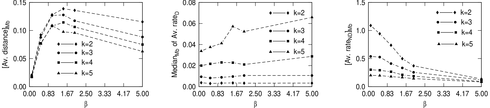
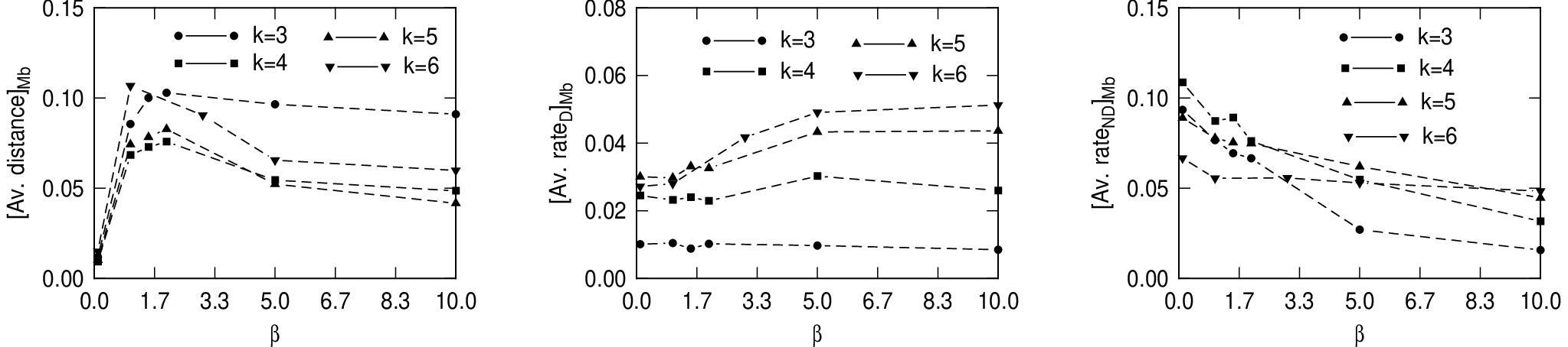
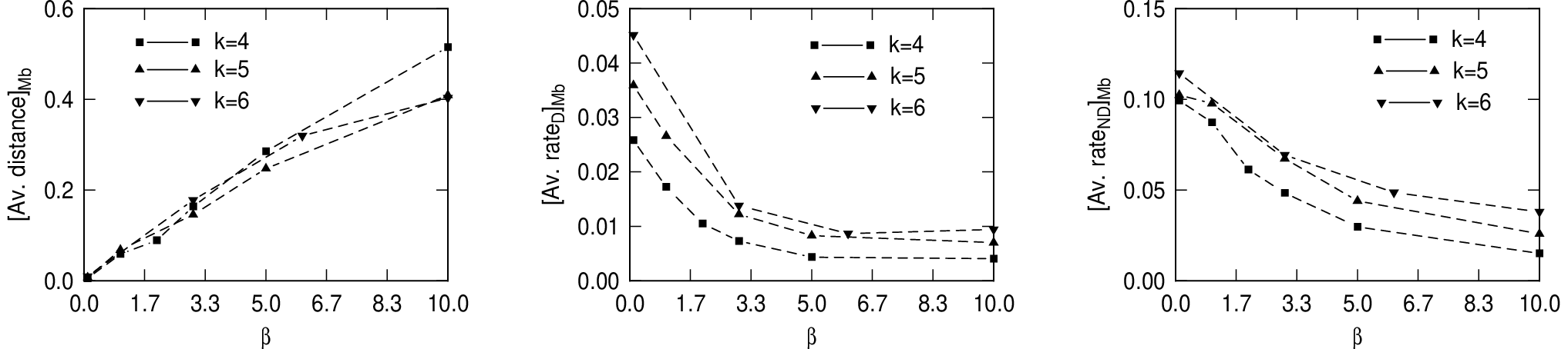
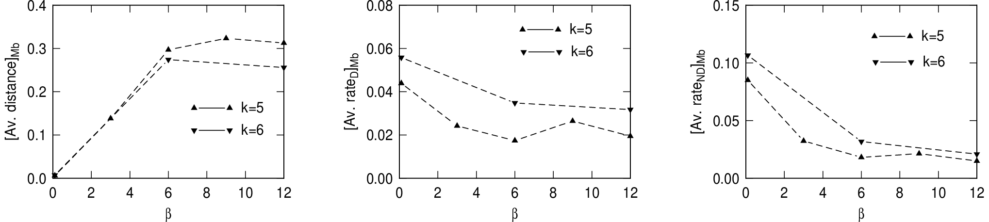
To study the dependence on and on the dimension of the bath versus the dimension of the system, we compute the following data. We pick a system Hamiltonian of qubits that has some well spread out spectrum. We set the dimension of the bath and then we randomly pick both the bath Hamiltonian and the interaction Hamiltonian. Means are denoted as . For the rates we look both at the mean and the median. The median is denoted as , see Fig. 5. The results for and are shown in Figs. 5-8. We have given the median when the mean does not give a good representation of the distribution.
These data clearly indicate that larger baths improve the process of equilibration, both in the rates (D and ND) as well as in the closeness to the equilibrium state. The effects are the most pronounced at low temperature, where equilibration is in general harder as the system must relax to a single pure ground state. To understand the closeness scale, we show in Appendix A how far apart two arbitrarily chosen density matrices are; this number lies around 1 for the dimensions that were considered. For these estimates, we see a trend towards approximations getting worse for larger system sizes for low temperature. The scaled rates and seem to be fairly constant, thus we see behavior that suggests that the rates are polynomially related to both system and bath number of qubits. We also observe that the nondiagonal rate (ND) is always higher than the diagonal rate (D). The data show a system Hamiltonian dependence, that is, the average equilibration for seems to be more succesful than for . We also observe that the difference between and becomes smaller with increasing (lower temperature). Thus, in conclusion, it seems if we pick a bath size (in number of qubits) that is polynomially related to the system size (note that the number of eigenvalues is then exponentially related), the rates of relaxation are polynomially related to the system size (in qubits); however the relaxed state could be still fairly far away from the true equilibrium state for large system sizes.
III Equilibration II
We present an alternative to the algorithm in section II. This algorithm relies on the technique for the estimation of eigenvalues, originally given in [2] (see [37, 38]). This eigenvalue estimation routine has also been used as a building block in an interesting quantum algorithm in [19] and [39].
Let be the -local Hamiltonian with non-degenerate eigenvalues as in section II. Order the eigenvalues as .
Definition 2
Equilibration algorithm II.
- 1.
Initialize the system in the (infinite temperature) completely mixed state . Also add one -qubit register set to .
- 2.
Compute eigenvalues with the use of the Fourier transform and dephase in computational eigenvalue basis, which will result in state
(131) where is a distribution, peaked at for large . The dephasing is a simple superoperator on the eigenvalue register that operates as
(132) - 3.
Prepare an additional -dimensional quantum system, the bath, also in . Add a -qubit register and one qubit register set to .
- 4.
Compute eigenvalues of the bath as for the system in step .
- 5.
Interact system and bath according the following rule (“partial swap”):
(133) where .
- 6.
Trace over the single-qubit register, all bath registers, and the eigenvalue register of the system. The system will be in some state
(134) The steps 2-6 define a map , .
- 7.
Repeat steps 2-6 times such that
(135) for all and is some accuracy.
The advantage of this algorithm is its simplicity and its similarity to a classical algorithm; we create a Markov chain in the eigenbasis of the system. The disadavantage of the algorithm is that it is very likely to be slow; the computation of the eigenvalues to high accuracy with the use of the Fourier transfrom is very likely to be exponential in the number of qubits of the system and has to be performed twice, for system and bath, in each round of the chain. First, let us show that in the case when the eigenvalues are computed exactly in steps and , i.e, the Markov chain equilibrates the system. Recall [37] that the routines of steps and compute rescaled eigenvalues
| (136) |
with and depending on the maximum and minimum eigenvalue (of which we assume that we can find an estimate) such that . In the following we will drop these primes. The chain that is created can be represented as
| (137) |
where . We have
| (138) |
Note that as required. The equilibrium state Eq. (1) obeys the detailed balance condition:
| (139) |
All the matrix elements of the Markov matrix are nonzero. Therefore the chain will have a unique fixed point which is equal to the equilibrium state due to detailed balance. Thus for all probability distributions we have
| (140) |
Notice that it is not hard to prepare the initial states of system and bath. One way to make the completely mixed state is to make a maximally entangled state and trace over the second register. This takes steps. The partial swap in step can be implemented with elementary qubit steps. The dephasing in step is introduced to keep the form of the algorithm clean, but it does not affect its output. This dephasing is implemented by measuring the eigenvalue register in the computational basis and discarding its answer. When using an -bit eigenvalue register the joint probability in the first round (after step ) is equal to
| (141) |
When is not a delta function on the eigenvalue, the Markov chain will still be in the eigenbasis of the system; It will be a concatenation of chains; the transition probability of this new chain is
| (142) |
where is a conditional probability, defined by , and is the exact chain (when ). Note that and , so that is a stochastic matrix. Let us make a few remarks about the behavior of such an approximate equilibration process. If this new Markov chain is close to the exact Markov chain, we can bound the deviation from the exact fixed point with perturbation theory [40]. Let
| (143) |
where is a deviation matrix defined by Eq. (142). Let where is the fixed point of the Markov chain . Assume that is diagonalizable. Let be the matrix defined as
| (144) |
where is the infinite iteration of . We can write in the basis where the stationary state is an eigenvector. In this basis, with diagonalizability, is of the form . We can then write
| (145) |
where is the second largest eigenvalue. For later use we note that the norm . It is possible to write the deviation in terms of and :
| (146) |
when is small enough such that is invertible. This expression can be derived from , which follows from the uniqueness of the stationary state . We now use
| (147) |
as in Proposition 41. Then using the expression for , Eq. (146) and Eq. (147) (see also below Eq. (47)) we can bound
| (148) |
Thus the size of the correction will be determined by the strength of the perturbation and the rate of convergence of the original Markov chain .
For a general , the computation of an -bit approximation of the eigenvalues is likely to cost an exponential (in ) number of elementary gates. As there are eigenvalues, knowing the bits of the values of still leaves groups of eigenvalues indistinguishable. Thus only in very special cases, if the gates can be implemented with a polynomial (in ) number of elementary steps (as in Shor’s factoring algorithm [1]) is it possible to compute the eigenvalues to high accuracy efficiently.
We have demonstrated a way to set up a Markov chain on a quantum computer that will converge to the equilibrium state for long enough time. For special Hamiltonians, there might be more efficient ways to tune and modify this kind of algorithm. The rule might be chosen to depend on other features of the eigenstates and as in the classical Metropolis algorithm where transitions are made between states that are related by local spin flips. There might be Hamiltonians for which the calculation of an eigenvalue, given the eigenvector, is efficient. Then there is the hard question of the (rapidly) mixing properties of the chain, that determines the computational efficiency of the algorithm.
IV (Time-dependent) observables
Given that we have prepared qubits in the equilibrium state corresponding to a certain Hamiltonian , we can then proceed by experimenting and measuring. The simplest measurement that we could try to perform is the estimation of the expectation value of a -local (Hermitian) observable :
| (149) |
As is local, we write where each operator operates on a Hilbert space of constant dimension . We can calculate the eigenvectors and eigenvalues of each rapidly on a (possibly) classical computer, which takes operations. If has eigenvalues that are both smaller as well as larger than zero, we define as
| (150) |
such that is positive semi-definite and has eigenvalues smaller than or equal than 1. If has only positive or zero eigenvalues, we just “normalize” the operator by dividing by , and similarly if has only negative eigenvalues. Let be a positive operator valued measurement (POVM [41]) with operation elements and and corresponding outcomes 1 and 2 such that
| (151) |
This measurement will give outcome 1 with probability
| (152) |
The operators and are given by
| (153) |
where is the diagonal form of and the diagonalizing matrix. We summarize these results in a Proposition:
Proposition 5
The estimation of where is a -local observable with precision and error-probability and () takes operations where is the time to prepare the state .
Proof: All commuting observables can be measured once for a single preparation of . To estimate a probability with precision and error probability we need samples [42]. .
More interesting is an algorithm to estimate time-dependent expectation values. Let and be two -local observables. We consider how to estimate a time-dependent quantity (identical to Eq. (10))
| (154) |
where is in the Heisenberg representation. Notice that , the time-evolved operator, will for general not be local. Thus we cannot use Proposition 5. The way these quantities come about in linear response theory [11] provides the key for how to estimate them on a quantum computer. One considers a system that is perturbed at some initial time : its time evolution is generated by the perturbed Hamiltonian () and is small. After time we consider the response of the system to the perturbation by measuring another observable . Notice that with Proposition 5, it is simple to perform this experiment. Linear response means that we take into account corrections of order , but no higher order, in the estimation of
| (155) |
where is the time-evolved system density matrix. This first-order correction takes the form [36]
| (156) |
If the disturbance we find on the right hand side the correlation function of Eq. (154). The quantity of Eq. (154) is interesting, because it can be used to compute the simplest reponse of the system, the linear response of Eq. (156), which we can directly estimate on our quantum computer, provided that both and are local. But we are of course not restricted to a linear response regime: is a parameter that we can tune freely. A sequence of measurements could determine higher response functions that will involve quantities such as
| (157) |
V Conclusion
It seems that by asking the question of how fast real quantum systems equilibrate, we have opened a Pandora’s box of hard-to-answer questions. If there are many simple quantum systems in nature that equilibrate slowly (that is, not in polynomial time) by any dynamics that does not require extensive preknowledge of the system, then it would be unreasonable to ask our quantum computer to perform this task efficiently. By relaxation in polynomial time we mean the following: in polynomial time we obtain a state that is within trace distance of the equilibrium state where is a small constant. It might be the case that leaving aside the classical phenomenon of frustration, relaxation does not take place in polynomial time. The idea here is that for a quantum system, the eigenbasis is not known beforehand, but must be singled out on the basis of an estimation of the eigenvalues, which is generically a hard problem.
This however is not in contradiction with physical and experimental reality as we know it, as the quantities that are measured in an experimental setup usually involve operators on a small number of qubits; these are the experiments that can be done efficiently (in polynomial time) and thus do not necessarily probe the system’s complete state. For example, the outcomes of the set of measurements where is one of the Pauli matrices or , completely determines the state, but there are measurements in this set. In an experimental setup, we might randomly select a polynomial subset of them and there is some small chance of order that these are the measurements that distinguish the equilibrated state from the present state in the lab that is supposed to approximate it. The estimates of time-dependent correlations could possibly be more sensitive to distance from equilibrium, as these involve time-evolved, non-local operations. The numerical study suggests that product baths whose size is polynomially related to the system can function as adequate baths in the sense of providing relaxation in polynomial time. The relaxed state could still be a rather rough approximation to the true equilibrium state, but, as we argued above, it might be a good starting point for subsequent measurements.
We have taken the bath to be part of the (cost of) the quantum computer. In any experimental setup, there is a natural bath that is used to equilibrate and cool the quantum computer. Can we use this bath for a computational problem such as equilibration? Consider for example the NMR quantum computer [18] where computation takes place at room temperature. In the regime in which the heat bath has a non-Markovian character it has been shown to be possible to alter the Hamiltonian of the system and the coupling to the bath dynamically (see [43], but also standard books on NMR [33]). These techniques could make it possible to simulate the time-evolution of a “designer” Hamiltonian and also to equilibrate the system to the equilibrium state of this designer Hamiltonian.
VI Acknowledgements
We would like to thank Charles Bennett, Daniel Loss, John Smolin, Ashish Thapliyal, Reinhard Werner, and Ronald de Wolf for stimulating discussions. DPD thanks support from the Army Research Office under contract number DAAG55-98-C-0041.
Appendix A Norms
In this Appendix we give the definitions of several norms and inner products. The inner product between vectors in can be represented on as
| (158) |
The trace norm [34, 35] is defined as
| (159) |
What makes this norm attractive is that it captures a measurable closeness of two density matrices and [35]:
| (160) |
where and are the probability distributions over outcomes that are obtained by measuring observable on and . The matrix norm is defined as
| (161) |
where is the Euclidean norm on : for . We have
| (162) |
In order to aid in the interpretation of the numerical results of section II.7, we present some numerical estimates for the average distance of two randomly chosen density matrices. We first have to choose a measure over . All density matrices can be written as with . The eigenvalues lie on a - dimensional simplex in . We use the Euclidean metric induced on the simplex. The Haar measure on the group of unitary matrices induces a uniform measure on the set of projectors . Together this defines a measure [44]. Within this measure, one can express the average distance between two density matrices and , using the unitary invariance of , as
| (163) |
Appendix B Preparation of the bath
To prepare the state
| (164) |
given , we first calculate the eigenvalues and eigenvectors of each qubit Hamiltonian . We prepare the state
| (165) |
with the eigenvalues of qubit Hamiltonian . This can be done by changing an initial state with probability into state for each . We then rotate each qubit to its eigenbasis :
| (166) |
In total we perform elementary qubit operations plus some constant classical overhead.
References
- [1] P. W. Shor, Proceedings of the 35th Annual Symposium on the Foundations of Computer Science (IEEE Press, Los Alamitos, CA 1994), p. 124.
- [2] A. Yu. Kitaev, e-print quant-ph/9511026.
- [3] L. K. Grover, Proc. of the 28th Annual ACM Symposium on Theory of Computing (ACM, Philadelphia, 1996), p.212.
- [4] D. Deutsch, Proc. Roy. Soc. Lond. A 400, 97 (1985).
- [5] S. Lloyd, Science 273, 1073 (1996).
- [6] C. Zalka, Proc. Roy. Soc. Lond. A 454, 313 (1998); S. Wiesner, quant-ph/9603028; B. M. Boghosian and W. Taylor, Physica D 120 (1998) 30-42.
- [7] J. M. Hammersley and D. C. Handscomb, Monte Carlo Methods (J.Wiley & Sons, London, 1964).
- [8] M. Suzuki, ed. Quantum Monte Carlo Methods in equilibrium and nonequilibrium systems, Springer Series in solid-state sciences (Springer-Verlag, Berlin, 1986).
- [9] H. De Raedt and W. von der Linden, Quantum Lattice Problems in The Monte Carlo Method in condensed matter physics, Topics in Applied Physics Vol. 71 (Springer-Verlag, Berlin, 1991).
- [10] M. Suzuki, Prog. Theor. Phys. 56, 1454 (1976).
- [11] S. Doniach and E. H. Sondheimer, Green’s functions for solid state physicists (Benjamin-Cummings, Reading, MA, 1974).
- [12] M. Jerrum and A. Sinclair, SIAM Journal of Computation Vol. 22, No.5, pp. 1087-1116 (1993).
- [13] F. Barahona, J. Physics. A 15, 3241 (1982).
- [14] In [15] quantum algorithms were presented to sample from the equilibrium distribution of arbitrary Ising spin glass models. The performance of these algorithms does not necessarily provide an exponential speedup over the best classical algorithms (see [12]) for the hard instances though.
- [15] D. Lidar and O. Biham, Phys. Rev. E 56, 3661 (1997).
- [16] D. S. Abrams and S. Lloyd, Phys. Rev. Lett. 79, 2586 (1997).
- [17] D. P. DiVincenzo, “Topics in quantum computers”, in Mesoscopic Electron Transport, Vol. 345 of NATO Advanced Study Institute, Series E: Applied Sciences, eds. L. Sohn, L. Kouwenhoven, and G. Schoen (Kluwer, Dordrecht, 1997), p. 657 and e-print cond-mat/9612126.
- [18] N. Gershenfeld and I. L. Chuang, Science 275, 350 (1997); D. Cory, A. Fahmy, and T. Havel, Proc. Nat. Acad. Sci. 94, 1634 (1997).
- [19] D. Abrams and S. Lloyd, e-print quant-ph/9807070.
- [20] E. Fick, G. Sauermann and W. D. Brewer, Quantum Statistics of Dynamic Processes, Springer Series in Solid-State Sciences Vol. 86 (Springer-Verlag, Berlin, 1990).
- [21] M. Celio and D. Loss, Physica A 158, 769-783 (1989).
- [22] R. Alicki and K. Lendi, Quantum dynamical semigroups and applications, Lec. Notes in Physics (Springer Verlag, Berlin, 1987).
- [23] G. Lindblad, Commun. Math. Phys. 48, 119-130 (1976).
- [24] E. B. Davies, Quantum Theory of Open Systems (Academic, New York, 1976).
- [25] E. B. Davies, Commun. Math. Phys. 39, 91-110 (1974).
- [26] E. B. Davies, Math. Annalen 219, 147-158 (1976).
- [27] R. Alicki, Rep. Math. Phys. 10, 249 (1976).
- [28] N. Dunford and J. T. Schwartz, Linear Operators, Part I (Interscience, New York, 1958).
- [29] R. F. Werner, private communication.
- [30] A. Messiah, Quantum Mechanics, Vol.II, Chapter XVI (J. Wiley & Sons, London, 1976).
- [31] R. A. Horn and C. R. Johnson, Matrix Analysis (Cambridge University Press, Cambridge, 1985).
- [32] cf. M. Jerrum and A. Sinclair, Approximation Algorithms for NP-hard Problems, edited by D. S. Hochbaum (PWS Publishing, Boston, 1996), pp. 482-520.
- [33] A. Abragam,The principles of nuclear magnetism (Oxford, Clarendon Press, 1961); R. R. Ernst, G. Bodenhausen and A. Wokaun, Principles of Nuclear Magnetic Resonance in One and Two Dimensions (Oxford, Clarendon Press, 1987). University Press, Oxford, 1961).
- [34] S. Richter and R. F. Werner, J. Stat. Phys. 82, 963 (1996).
- [35] D. Aharonov, A. Kitaev, N. Nissan, Proceedings of the 30th Annual ACM Symposium on Theory of Computation (ACM, Philadelphia, 1997), pp. 20-30.
- [36] A. L. Fetter and J. D. Walecka, Quantum Theory of many-particle systems (McGraw-Hill Book Company, New York, 1971).
- [37] R. Cleve, A. Ekert, C. Macchiavello and M. Mosca, Proc. Roy. Soc. Lond. A 454, 339 (1998).
- [38] R. Jozsa, Proc. R. Soc. Lond. A 454, 323 (1998).
- [39] D. A. Lidar and H. Wang, Phys. Rev. E 59 (1999) 2429.
- [40] cf. G. W. Stewart and Ji-guang Sun, Matrix Perturbation Theory, Computer science and scientific computing (Academic, San Diego, 1990); P. J. Schweitzer, Journal of Appl. Prob. 5, 401 (1968); M. Haviv and L. van der Heyden, Adv. Appl. Prob. 16, 804 (1984).
- [41] A. Peres, Quantum Theory: Concepts and Methods (Kluwer, Dordrecht, 1993).
- [42] W. Feller, An Introduction to Probability Theory and Its Application Vol I (J. Wiley & Sons, London, 1968).
- [43] L. Viola, E. Knill and S. Lloyd, “Dynamical Decoupling of Open Quantum Systems”, quant-ph/9809071.
- [44] K. Zyczkowski, P. Horodecki, A. Sanpera and M. Lewenstein, Phys. Rev. A 58, 883 (1998).
| dimension | N | K | ||
| locality | 4 | 4 | ||
| sampling scale a | 1 | 1 | 1 |


| dim N | mean | standard error, |
|---|---|---|
| 4 | 0.90388 | 0.00740588 |
| 8 | 0.96190 | 0.00514057 |
| 16 | 1.00294 | 0.00341226 |
| 32 | 1.01452 | 0.00220363 |
| 64 | 1.02617 | 0.00132233 |