Floquet-Markov description of the parametrically driven, dissipative harmonic quantum oscillator

Sigmund Kohler Thomas Dittrich Note: Present address: Max-Planck-Institut für Physik komplexer Systeme, Bayreuther Straße 40, Haus 16, D–01187 Dresden, Germany and Peter Hänggi Address: Institut für Physik, Universität Augsburg, Memminger Straße 6, D–86135 Augsburg, Germany

August 11, 2026

Abstract

Using the parametrically driven harmonic oscillator as a working example, we study two different Markovian approaches to the quantum dynamics of a periodically driven system with dissipation. In the simpler approach, the driving enters the master equation for the reduced density operator only in the Hamiltonian term. An improved master equation is achieved by treating the entire driven system within the Floquet formalism and coupling it to the reservoir as a whole. The different ensuing evolution equations are compared in various representations, particularly as Fokker-Planck equations for the Wigner function. On all levels of approximation, these evolution equations retain the periodicity of the driving, so that their solutions have Floquet form and represent eigenfunctions of a non-unitary propagator over a single period of the driving. We discuss asymptotic states in the long-time limit as well as the conservative and the high-temperature limits. Numerical results obtained within the different Markov approximations are compared with the exact path-integral solution. The application of the improved Floquet-Markov scheme becomes increasingly important when considering stronger driving and lower temperatures.

pacs

05.30.-d, 42.50.Lc, 03.65.Sq

I Introduction

The dynamics of microscopic systems in strong periodic fields forms a problem of fundamental significance, with a vast variety of applications in quantum optics, quantum chemistry, and mesoscopic systems. If the driving field is of a macroscopic nature, for example, a continuous-wave laser irradiation, it is appropriate to describe the complete system in a mixed quantum-classical way, i.e., to give a full quantum-mechanical account of the central system and its energy loss to ambient degrees of freedom (the electromagnetic vacuum or weakly coupled internal degrees of freedoms), but to include the field as a classical external driving force. A solution of the dynamics then requires to simultaneously eliminate the ambient freedoms and to integrate the equations of motion with an explicit time dependence. In principle, this can be done exactly using path-integral techniques. However, even a partially analytical solution within the path-integral approach is feasible only for the very simplest systems in the class addressed, in particular, for periodically driven, damped harmonic oscillators [1], or for driven dissipative two-level systems [2]. As soon as nonlinear forces come into play, the path-integral approach requires to resort to extensive and sophisticated numerics, such as Monte-Carlo calculations [3], with their own shortcomings.

In most cases of interest, it is more adequate to make as much use as possible of the methods and approximations that have been developed separately for the two problems mentioned above, quantum dissipation on the one hand and periodic driving on the other. Specifically, it is desirable to combine a Markovian approach to quantum dissipation, leading to a master equation for the density operator, with the Floquet formalism that allows to treat time-periodic forces of arbitrary strength and frequency. While the Floquet formalism amounts essentially to using an optimal representation and is exact [4], the simplification brought about by the Markovian description is achieved only on the expense of accuracy. Here, a subtle technical difficulty lies in the fact that the truncation of the long-time memory introduced by the bath, and the inclusion of the driving, do not commute: As pointed out in Ref. [5], the result of the Markov approximation depends on whether it is made with respect to the eigenenergy spectrum of the central system without the driving, or with respect to the quasienergy spectrum obtained from the Floquet solution of the driven system. In the second case it cannot be treated as a system with proper eigenstates and eigenenergies. A Markovian approach based on a quasienergy spectrum has been implemented in recent work on driven Rydberg atoms [6] and driven dissipative tunneling [7].

The purpose of the present paper is to investigate these two Markovian approaches to damped periodically driven quantum dynamics, with their specific merits and drawbacks, for a linear system where an exact path-integral solution is still available: The parametrically driven, damped harmonic oscillator allows for a very transparent and well-controlled introduction of the different approximation schemes at hand. Their quality can here be reliably checked since in this system, the quasienergy spectrum is sufficiently different from the unperturbed energy spectrum [8] (this feature is in contrast to the additively driven harmonic oscillator, where the difference of two quasienergies does not depend on the driving parameters [8]), and a comparison with the known quantum path-integral solution [1] is possible.

Moreover, by switching to a phase-space representation such as the Wigner function, it is possible to elucidate the relationship of the quantal results to the corresponding classical Liouville dynamics. Since this relation is particularly close in the case of linear systems, this provides an additional consistency check. Therefore, the emphasis of this paper is predominantly on the testing and thorough understanding of the available methods. Their application to a strongly nonlinear system where analytical path-integral solutions are far beyond our present capabilities, will be the subject of forthcoming publications.

Forming a convenient “laboratory animal” due to its simplicity and linearity, the parametrically driven harmonic oscillator still shows nontrivial behaviour, interesting in its own right. We shall give a brief review of the model and its classical dynamics in Section II. The central results of the paper, concerning the applicability and quality of the alternative Markov approximations, are presented in the course of the quantization of the system with dissipation, in Section III. Its last subsection is devoted to a discussion of the asymptotics of the quantal solutions, such as the conservative and the high-temperature limits. Section IV contains numerical results for a number of characteristic dynamical quantities as obtained for the alternative Markovian approaches, and the comparison to the path-integral solution. A summary of the various representations and levels of description addressed in the paper, with their interrelations, is given in Section V. A number of technical issues are deferred to Appendix A. Results for an additive time-dependent force in combination with a parametric periodic driving are summarized in Appendix B.

II The model and its classical dynamics

For a particle with mass $m$ moving in a harmonic potential with time-dependent frequency, the Hamiltonian is given by

H_{\rm S}(t)=\frac{p^{2}}{2m}+\frac{1}{2}k(t)x^{2},

(1)

where $k(t)$ is a symmetric and periodic function with period $T$ . A special case is the Mathieu oscillator, where $k(t)=m(\omega_{0}^{2}+\varepsilon\cos\Omega t)$ with $\Omega=2\pi/T$ . Depending on its frequency and amplitude, the driving can stabilize or destabilize the undriven oscillation. Fig. 1 shows the zones of stable and unstable motion, respectively, for the Mathieu oscillator, in the $\omega_{0}^{2}$ – $\varepsilon$ –plane. The equation of motion for a classical particle with velocity–proportional (i.e., Ohmic) dissipation in the potential given in (1) reads

\ddot{x}+\gamma\dot{x}+\frac{1}{m}k(t)x=0.

(2)

By substituting $x=y\exp(-\gamma t/2)$ , we can formally remove the damping to get an undamped equation with a modified potential

\ddot{y}+\left(k(t)/m-\gamma^{2}/4\right)y=0.

(3)

Already here, on the level of the classical equations of motion, we can apply the Floquet theorem for second-order differential equations with time-periodic coefficients. It asserts [9] that Eq. (3) has two solutions of the form

\xi_{1}(t)={\rm e}^{{\rm i}\mu t}\varphi(t),\quad\xi_{2}(t)=\xi_{1}(-t),\quad\varphi(t+T)=\varphi(t).

(4)

The solution $\xi_{2}(t)$ is related to $\xi_{1}(t)$ by the time-inversion symmetry inherent in (3). Being periodic in time, the classical Floquet function $\varphi(t)$ can be represented as a Fourier series

\varphi(t)=\sum_{n=-\infty}^{\infty}c_{n}{\rm e}^{{\rm i}n\Omega t}.

(5)

The Floquet index $\mu$ depends on the shape of the driving $k(t)$ and is defined only ${\,\rm mod\,}\Omega$ . There exist driving functions for which $\mu$ is complex so that one of the solutions $\xi_{i}(t)$ becomes unstable (cf. Fig. 1). In stable regimes $\mu$ is real. On the border between a stable and an unstable regime, $\mu$ becomes a multiple of $\Omega/2$ and the solutions $\xi_{1}(t)$ and $\xi_{2}(t)$ are not linearly independent. For given $k(t)$ , the $\xi_{i}(t)$ still depend on the damping $\gamma$ . We denote the limit $\gamma\to 0$ of the functions $\xi_{i}(t)$ by $\xi^{0}_{i}(t)$ .

The normalization of the $c_{n}$ is chosen such that the Wronskian $\cal W$ , which is a constant of motion, is given by

{\cal W}=\dot{\xi}_{1}(t)\xi_{2}(t)-\xi_{1}(t)\dot{\xi}_{2}(t)=2{\rm i},

(6)

resulting in the sum rule

\sum_{n=-\infty}^{\infty}c_{n}^{2}(\mu+n\Omega)=1.

(7)

Returning to the original $x$ –coordinate, we find that the fundamental solutions of (2) read

f_{i}(t)={\rm e}^{-\gamma t/2}\xi_{i}(t),\qquad i=1,2.

(8)

For constant frequency of the oscillator, $k(t)={\rm const}=m\omega_{0}^{2}$ , the Floquet index and the periodic function become $\mu=(\omega_{0}^{2}-\gamma^{2}/4)^{1/2}$ and $\varphi(t)=(\omega_{0}^{2}-\gamma^{2}/4)^{-1/2}$ , respectively, which reproduces the results for a damped harmonic oscillator without driving.

The Green function for Eq. (2) is constructed using Eqs. (5) and (6),

	$\displaystyle G(t,t^{\prime})$	$\displaystyle=$	$\displaystyle{\rm e}^{-\gamma(t-t^{\prime})/2}\left[\xi_{1}(t)\xi_{2}(t^{\prime})-\xi_{2}(t)\xi_{1}(t^{\prime})\right]/2{\rm i}$		(9)
		$\displaystyle=$	$\displaystyle{\rm e}^{-\gamma(t-t^{\prime})/2}\sum_{n,n^{\prime}}c_{n}c_{n^{\prime}}\sin\left[\mu(t-t^{\prime})+\Omega(nt-n^{\prime}t^{\prime})\right].$		(10)

In terms of this function, the solution of (2) with initial conditions $x(t_{0})=x_{0}$ and $p(t_{0})=p_{0}$ , reads

x(t,t_{0})=-x_{0}\frac{\partial G(t,t_{0})}{\partial t_{0}}+\frac{p_{0}}{m}G(t,t_{0}).

(11)

Since the potential breaks continuous time-translational invariance, this solution depends explicitly on the initial time $t_{0}$ .

III The dissipative quantum system

To achieve a microscopic model of dissipation, we couple the system (1) bilinearly to a bath of non-interacting harmonic oscillators [10]. The total Hamiltonian of system and bath is then given by

\hat{H}(t)=\hat{H}_{\rm S}(t)+\hat{H}_{\rm SB}+\hat{H}_{\rm B},

(12)

where

\hat{H}_{\rm B}=\sum_{\nu=1}^{N}\left(\frac{\hat{p}_{\nu}^{2}}{2m_{\nu}}+\frac{m_{\nu}}{2}\omega_{\nu}^{2}\hat{x}_{\nu}^{2}\right)

(13)

is the Hamiltonian of $N$ oscillators with masses $m_{\nu}$ , frequencies $\omega_{\nu}$ , momenta $\hat{p}_{\nu}$ , and coordinates $\hat{x}_{\nu}$ . The bath interacts with the system via

\hat{H}_{\rm SB}=-\hat{x}\sum_{\nu=1}^{N}g_{\nu}\hat{x}_{\nu}+\hat{x}^{2}\sum_{\nu=1}^{N}\frac{g_{\nu}^{2}}{2m_{\nu}\omega_{\nu}^{2}},

(14)

which couples the system to each bath oscillator $\nu$ with a strength $g_{\nu}$ . The second term in Eq. (14) serves to cancel a shift of the potential minimum due to the coupling [10, 11]. The bath is fully characterized by the spectral density of the coupling energy,

I(\omega)=\pi\sum_{\nu=1}^{N}\frac{g_{\nu}^{2}}{2m_{\nu}\omega_{\nu}}\delta(\omega-\omega_{\nu}).

(15)

We choose an initial condition of the Feynman-Vernon type, i.e., at $t=t_{0}$ the bath is in thermal equilibrium and uncorrelated to the system, i.e.

\rho(t_{0})=\rho_{\rm S}(t_{0})\otimes\rho_{\rm B,eq},

(16)

where $\rho_{\rm B,eq}=\exp(-\hat{H}_{\rm B}/k_{\rm B}T)/{\rm tr}_{\rm B}\exp(-\hat{H}_{\rm B}/k_{\rm B}T)$ is the canonical ensemble of the bath and $k_{\rm B}T$ Boltzmann’s constant times temperature.

III.1 Interaction picture and perturbation theory

Due to the bilinearity of the system-bath coupling, one can always eliminate the bath variables to get an exact, closed integro-differential equation for the reduced density matrix $\rho_{\rm S}={\rm tr}_{\rm B}\rho$ , which describes the dynamics of the central system, subject to dissipation [12, 13, 14]. In most cases, however, this equation cannot be solved exactly. In the limit of weak coupling,

	$\displaystyle\gamma$	$\displaystyle\ll$	$\displaystyle k_{\rm B}T/\hbar,$		(17)
	$\displaystyle\gamma$	$\displaystyle\ll$	$\displaystyle\Delta_{\alpha\beta},$		(18)

it is possible to truncate the time-dependent perturbation expansion in the system-bath interaction after the second-order term. The quantity $\gamma$ denotes the effective damping of the dissipative system, and $\Delta_{\alpha\beta}$ are the transition frequencies of the central system (see, e.g. Eq. (56), below). The autocorrelations of the bath decay on a time scale $\hbar/k_{\rm B}T$ , and thus in this limit instantaneously on the time scale $1/\gamma$ of the system correlations.

With the initial preparation (16), the equation of motion for the reduced density matrix in this approximation is given by [12, 13, 14]

	$\displaystyle\dot{\rho}_{\rm S}(t)$	$\displaystyle=$	$\displaystyle-\frac{{\rm i}}{\hbar}\left[\hat{H}_{\rm S}(t),\rho_{\rm S}(t)\right]-\frac{{\rm i}}{\hbar}{\rm tr}_{\rm B}\left[\hat{H}_{\rm SB},\rho_{\rm S}(t)\right]$		(19)
			$\displaystyle-\frac{1}{\hbar^{2}}\int_{0}^{\infty}{\rm d}\tau\,{\rm tr}_{\rm B}\left[\hat{H}_{\rm SB},\left[\tilde{H}_{\rm SB}(t-\tau,t),\rho_{\rm B,eq}\otimes\rho_{\rm S}(t)\right]\right].$		(19)

The tilde denotes the interaction picture defined by

	$\displaystyle\tilde{\cal O}(t,t^{\prime})$	$\displaystyle=$	$\displaystyle U_{0}^{\dagger}(t,t^{\prime})\hat{\cal O}U_{0}(t,t^{\prime}),$		(20)
	$\displaystyle U_{0}(t,t^{\prime})$	$\displaystyle=$	$\displaystyle{\cal T}\exp\left(-\frac{{\rm i}}{\hbar}\int_{t^{\prime}}^{t}{\rm d}t^{\prime\prime}(\hat{H}_{\rm S}(t^{\prime\prime})+\hat{H}_{\rm B})\right),$		(21)

where ${\cal T}$ is Wick’s time-ordering operator.

For $\hat{H}_{\rm S}$ and $\hat{H}_{\rm SB}$ as in Eqs. (13), (14), we find the master equation

$\displaystyle\dot{\rho}_{\rm S}(t)$	$\displaystyle=$	$\displaystyle-\frac{{\rm i}}{\hbar}\left[\hat{H}_{\rm S}(t),\rho_{\rm S}(t)\right]$	(22)
		$\displaystyle-\frac{1}{\hbar^{2}}\sum_{\nu=1}^{N}g_{\nu}^{2}\int_{0}^{\infty}{\rm d}\tau\Big\{S_{\nu}(\tau)\big[\hat{x},\big[\tilde{x}(t-\tau,t),\rho_{\rm S}(t)\big]\big]$
		$\displaystyle\qquad\qquad\qquad+{\rm i}A_{\nu}(\tau)\big[\hat{x},\big[\tilde{x}(t-\tau,t),\rho_{\rm S}(t)\big]_{+}\big]\Big\},$

with $[A,B]_{+}=AB+BA$ and

	$\displaystyle S_{\nu}(t)$	$\displaystyle=$	$\displaystyle\frac{\hbar}{2m_{\nu}\omega_{\nu}}\coth\left(\frac{\hbar\omega_{\nu}}{2k_{\rm B}T}\right)\cos\omega_{\nu}t,$		(23)
	$\displaystyle A_{\nu}(t)$	$\displaystyle=$	$\displaystyle-\frac{\hbar}{2m_{\nu}\omega_{\nu}}\sin\omega_{\nu}t,$		(24)

the symmetrically ordered and antisymmetrically ordered, respectively, correlation functions of the bath oscillator $\nu$ .

III.2 Markov approximation with respect to the unperturbed spectrum

So far, we have followed the standard approach to dissipative quantum dynamics in the weak coupling limit [12, 13, 14]. In the following subsections, we shall contrast a simpler Markov approximation based on the unperturbed spectrum, with a more sophisticated approach that accounts for the modification of the spectrum due to the driving.

III.2.1 Master equation

In the following, we restrict ourselves to an ohmic bath,

I(\omega)=m\gamma\omega,

(25)

fixing the relation between the macroscopic damping constant $\gamma$ and the microscopic coupling constants $g_{n}$ introduced in Eq. (14). By imposing a Drude cutoff $I(\omega)\to I(\omega)/(1-{\rm i}\omega/\omega_{\rm D})$ with $\omega_{\rm D}\gg\omega_{0},\Omega$ , divergent integrals are avoided.

In a crudest approximation, the time dependence of the system Hamiltonian is neglected in the derivation of the master equation, i.e., the incoherent terms in the master equation are calculated replacing $\hat{H}_{\rm S}(t)$ by $\bar{H}_{\rm S}=(1/T)\int_{0}^{T}{\rm d}t\,\hat{H}_{\rm S}(t)$ , i.e. the Hamiltonian with zero driving amplitude. The position operator in the interaction picture is then given by

\tilde{x}(t,t^{\prime})=\hat{x}\cos\omega_{0}(t-t^{\prime})+\frac{\hat{p}}{m\omega_{0}}\sin\omega_{0}(t-t^{\prime}).

(26)

Since the information on the phase of the driving is lost, it depends only on the difference $t-t^{\prime}$ of its arguments.

Inserting this operator and the correlation functions (23), (24) into Eq. (22), leads to the master equation

	$\displaystyle\dot{\rho}_{\rm S}$	$\displaystyle=$	$\displaystyle-\frac{{\rm i}}{\hbar}\big[\hat{H}_{\rm S}(t),\rho_{\rm S}\big]-\frac{{\rm i}}{2\hbar}\bar{\gamma}\ [\hat{x},[\hat{p},\rho_{\rm S}]_{+}]$		(27)
			$\displaystyle-\frac{\gamma}{\hbar^{2}}D_{pp}[\hat{x},[\hat{x},\rho_{\rm S}]]+\frac{\gamma}{\hbar^{2}}D_{xp}[\hat{x},[\hat{p},\rho_{\rm S}]].$		(27)

The right-hand side of this equation depends on time only through its first, the Hamiltonian, term and therefore retains the periodicity of the system Hamiltonian $\hat{H}_{\rm S}(t)$ .

This form of the master equation does not produce a positive semidefinite diffusion matrix. It consequently does not exhibit Lindblad form [13, 15, 16, 17]. The positivity of $\rho_{\rm S}$ is thus not guaranteed for all elements of the function space of density operators. The Markovian approximation implies that quantum effects on a length scale $l<\lambda_{\rm dB}=\hbar/\sqrt{4mk_{\rm B}T}$ (non-Markov effects) cannot be described selfconsistently [17, 18, 19]. Note also that within a Markov approximation, the master equation is periodic with the driving period $T=2\pi/\Omega$ (Floquet form). This is in contrast to the non-Markovian exact master equation [1]. In this latter case, the effective master equation has the structure of (27) with time-dependent coefficients $D_{xp}$ and $D_{pp}$ that depend also in a non-periodic way on the time elapsed since the preparation at $t_{0}$ . In Wigner representation, this corresponds to a time-dependent diffusion coefficient (see below).

The coefficients $\bar{\gamma}$ and $D_{pp}$ can be evaluated straightforwardly [20] to give

	$\displaystyle\bar{\gamma}$	$\displaystyle=$	$\displaystyle\gamma,$		(28)
	$\displaystyle D_{pp}$	$\displaystyle=$	$\displaystyle\frac{1}{2}m\hbar\omega_{0}\coth\frac{\hbar\omega_{0}}{2k_{\rm B}T}.$		(29)

The evaluation of the cross-diffusion $D_{xp}$ is more complex. Because we did not find it in the literature, we give the outline of its derivation. The logarithmic divergence of $D_{xp}$ is regularized by the Drude cutoff to obtain

D_{xp}=-\frac{\hbar}{2\pi}{\rm P}\int_{-\infty}^{\infty}{\rm d}\omega\coth\left(\frac{\hbar\omega}{2k_{\rm B}T}\right)\frac{\omega}{\omega^{2}-\omega_{0}^{2}}\;\frac{{\rm i}\omega_{\rm D}}{\omega+{\rm i}\omega_{\rm D}},

(30)

where P denotes Cauchy’s principal part. The integral in Eq. (30) is solved by contour integration in the upper half plane. Expressing the resulting sums by the psi function $\psi(x)={\rm d}\ln\Gamma(x)/{\rm d}x$ [21] and neglecting terms of the order $\omega_{0}/\omega_{\rm D}$ , we obtain

D_{xp}=-\frac{\hbar}{\pi}\left[\psi\left(1+{\hbar\omega_{\rm D}\over 2\pi k_{\rm B}T}\right)+C\right],

(31)

where $C$ is the Euler constant.

Interestingly enough, $m\gamma D_{xp}$ coincides with the Drude regularized divergent part of the stationary momentum variance of a dissipative harmonic oscillator [22].

It must be stressed that the dissipative terms in the master equation (27) are independent of the driving. This manifestly reflects that the time dependence of $H_{\rm S}(t)$ has not been taken into account in the incoherent terms of the master equation.

III.2.2 Wigner representation and Fokker-Planck equation

In order to achieve a description close to the classical phase-space dynamics, we discuss the time evolution of the density operator in Wigner representation. It is defined by [23]

W(x,p,t)=\frac{1}{\pi\hbar}\int_{-\infty}^{\infty}{\rm d}x^{\prime}{\rm e}^{{2\rm i}px^{\prime}/\hbar}\langle x-x^{\prime}|\rho_{\rm S}(t)|x+x^{\prime}\rangle.

(32)

The moments of the Wigner function are the symmetrically-ordered expectation values of the density operator.

Applying this transformation to the master equation (22), we obtain a c-number equation of motion,

\partial_{t}W(x,p,t)=L(t)W(x,p,t),

(33)

with the differential operator

L(t)=-{1\over m}p\partial_{x}+\gamma\partial_{p}p+k(t)x\partial_{p}+\gamma D_{pp}\partial_{p}^{2}+\gamma D_{xp}\partial_{x}\partial_{p}.

(34)

Equation (34) has the structure of an effective Fokker-Planck operator. However, for $D_{xp}\neq 0$ , the diffusion matrix is not positive semidefinite; correspondingly (33) has no equivalent Langevin representation.

As is the case for the master equation from which it has been derived, the coefficients of the Fokker-Planck operator retain the it periodicity of the driving, so that Eq. (33) has solutions of Floquet form. This fact will be exploited in the following subsection to construct the solutions.

III.2.3 Wigner-Floquet solutions

The Fokker-Planck equation for the density operator in Wigner representation, Eq. (33) with Eq. (34), offers the opportunity to make full use of the well-known and intuitive results for the corresponding classical stochastic system. In particular, a solution of the Fokker-Planck equation can be obtained directly by solving the equivalent Langevin equation [24, 25], or by using the formula for the conditional probability of a Gauss process [25]. In the present case, however, the fact that the diffusion matrix of (34) is not positive semidefinite requires to take a different route.

Since Eq. (33) with Eq. (34) represents a differential equation with time-periodic coefficients, it complies with the conditions of the Floquet theorem. Consequently, there exists a complete set of solutions of the form

W_{\alpha}(x,p,t)={\rm e}^{\mu_{\alpha}t}u_{\alpha}(x,p,t),\quad u_{\alpha}(x,p,t)=u_{\alpha}(x,p,t+T),

(35)

henceforth referred to as Wigner-Floquet functions.

We construct a solution for (33) of this form with $\mu_{00}=0$ by the method of characteristics [26], cf. the Appendix A. In the limit $t_{0}\to-\infty$ , the terms in the first line of (116), which contain the initial condition, vanish and we obtain the asymptotic solution

W_{00}(x,p,t)=\frac{1}{2\pi}\left|\begin{array}[]{cc}\sigma_{xx}(t)&\sigma_{xp}(t)\\ \sigma_{xp}(t)&\sigma_{pp}(t)\end{array}\right|^{-1/2}\exp\left\{-\frac{1}{2}\left(\begin{array}[]{c}x\\ p\end{array}\right)\left(\begin{array}[]{cc}\sigma_{xx}(t)&\sigma_{xp}(t)\\ \sigma_{xp}(t)&\sigma_{pp}(t)\end{array}\right)^{-1}\left(\begin{array}[]{c}x\\ p\end{array}\right)\right\}

(36)

with the variances

$\displaystyle\sigma_{xx}(t)$	$\displaystyle=$	$\displaystyle\frac{2\gamma D_{pp}}{m^{2}}\int_{-\infty}^{t}{\rm d}t^{\prime}\left[G(t,t^{\prime})\right]^{2},$	(37)
$\displaystyle\sigma_{xp}(t)$	$\displaystyle=$	$\displaystyle\frac{2\gamma D_{pp}}{m}\int_{-\infty}^{t}{\rm d}t^{\prime}G(t,t^{\prime})\frac{\partial}{{\partial}t}G(t,t^{\prime}),$	(38)
$\displaystyle\sigma_{pp}(t)$	$\displaystyle=$	$\displaystyle-m\gamma D_{xp}+2\gamma D_{pp}\int_{-\infty}^{t}{\rm d}t^{\prime}\left[\frac{\partial}{{\partial}t}G(t,t^{\prime})\right]^{2}.$	(39)

Note that in (37)–(39) the difference in using $D_{pp}$ and $D=D_{pp}+\gamma D_{xp}$ (see (112) in Appendix A) is meaningless, since it is a correction of order $\gamma$ . By inserting for $G(t,t^{\prime})$ the Fourier representation (10), one finds that the variances are asymptotically time-periodic.

Starting from $W_{00}$ , we construct further Wigner-Floquet functions: By solving the characteristic equations (see Appendix A), we find the two time-dependent differential operators

	$\displaystyle Q_{1+}(t)$	$\displaystyle=$	$\displaystyle f_{1}(t)\partial_{x}+m\dot{f}_{1}(t)\partial_{p},$		(40)
	$\displaystyle Q_{2+}(t)$	$\displaystyle=$	$\displaystyle f_{2}(t)\partial_{x}+m\dot{f}_{2}(t)\partial_{p}.$		(41)

They have the properties

\left[L(t)-\partial_{t},Q_{1+}(t)\right]=\left[L(t)-\partial_{t},Q_{2+}(t)\right]=0

(42)

and

	$\displaystyle Q_{1+}(t+T)$	$\displaystyle=$	$\displaystyle{\rm e}^{(-\gamma/2+{\rm i}\mu)T}Q_{1+}(t),$		(43)
	$\displaystyle Q_{2+}(t+T)$	$\displaystyle=$	$\displaystyle{\rm e}^{(-\gamma/2-{\rm i}\mu)T}Q_{2+}(t).$		(44)

Taking the commutation relation (42) into account, the functions

W_{nn^{\prime}}(x,p,t)=Q_{1+}^{n}(t)Q_{2+}^{n^{\prime}}(t)W_{00}(x,p,t),\quad n,n^{\prime}=0,1,2,\ldots

(45)

also solve Eq. (33).

Due to Eqs. (43), (44), they are of Floquet structure with the Floquet spectrum

\mu_{nn^{\prime}}=n(-\gamma/2+{\rm i}\mu)+n^{\prime}(-\gamma/2-{\rm i}\mu).

(46)

This spectrum is independent of the diffusion constants, as expected for an operator of type (34) [27], and therefore is the same as in the case of classical parametrically driven Brownian oscillator [28].

The expression for the eigenfunctions in the high-temperature limit of the (undriven) classical Brownian harmonic oscillator in Refs. [27, 29] is also of the structure (45). We can recover this solution by inserting the classical diffusion constant $mk_{\rm B}T$ and the undriven limit $\varepsilon\to 0$ for the classical solution, given in Sect. II.

III.3 Markov approximation with respect to the quasienergy spectrum

The master equation (27) can be improved by including the time-dependent term in the system Hamiltonian (1) before a Markov approximation is introduced, to account for the change in the quasienergy spectrum due to the driving.

III.3.1 Floquet theory and quasienergy spectrum

For a Schrödinger equation with time-periodic system Hamiltonian such as (1), the Floquet theorem [4] asserts that there exists a complete set of solutions of the form

|\psi_{\alpha}(t)\rangle={\rm e}^{-{\rm i}\mu_{\alpha}t}|\phi_{\alpha}(t)\rangle,\quad|\phi_{\alpha}(t+T)\rangle=|\phi_{\alpha}(t)\rangle

(47)

The quasienergy $\mu_{\alpha}$ plays the role of a phase and therefore is only defined ${\,\rm mod\,}\Omega$ , cf. Ref. [4]. We shall use the basis $\{|\psi_{\alpha}(t)\rangle\}$ as an optimal representation to decompose states and operators.

For the parametrically driven harmonic oscillator (1), the Floquet solutions for the Schrödinger equation are derived in the literature in various ways [30, 31, 32, 33]. We skip the derivation and merely present the result,

\psi_{\alpha}(x,t)=\left(\frac{\sqrt{m/\pi\hbar}}{2^{\alpha}n!\xi^{0}_{1}(t)}\right)^{1/2}\left(\frac{\xi^{0}_{1}(t)}{\xi^{0}_{2}(t)}\right)^{\alpha/2}H_{\alpha}\left(x\sqrt{m/\hbar\xi^{0}_{1}(t)\xi^{0}_{2}(t)}\right)\exp\left({\rm i}{\dot{\xi}^{0}_{1}(t)x^{2}}/2{\xi^{0}_{1}(t)}\right),

(48)

for the Floquet solutions in the stable regime, where $H_{\alpha}$ is the $\alpha$ -th Hermite polynomial, $\alpha=0,1,2,\ldots$ . The Floquet index for this solution is $\mu_{\alpha}=\mu(\alpha+1/2)$ . This gives the quasienergy spectrum

\mu_{\alpha,k}=(\alpha+1/2)\mu^{0}+k\Omega,\quad k=0,\pm 1,\pm 2,\ldots.

(49)

Note that (48) are solutions only in the stable regime. Consequently $\mu$ is real, cf. Sect. II.

In analogy to the annihilation and creation operators for the undriven harmonic oscillator, one can define operators $\hat{\Gamma}$ and $\hat{\Gamma}^{\dagger}$ which act as shift operators for the Floquet states, i.e.

	$\displaystyle\hat{\Gamma}(t)\|\psi_{\alpha}(t)\rangle$	$\displaystyle=$	$\displaystyle\sqrt{\alpha}\,\|\psi_{\alpha-1}(t)\rangle,$		(50)
	$\displaystyle\hat{\Gamma}^{\dagger}(t)\|\psi_{\alpha}(t)\rangle$	$\displaystyle=$	$\displaystyle\sqrt{\alpha+1}\,\|\psi_{\alpha+1}(t)\rangle.$		(51)

For a parametrically driven harmonic oscillator, $\hat{\Gamma}(t)$ can be expressed in terms of position and momentum operator as [31, 32]

\hat{\Gamma}(t)=\frac{1}{2\rm i}\left(\hat{x}\sqrt{\frac{2m}{\hbar}}\dot{\xi}_{1}^{0}(t)-\hat{p}\sqrt{\frac{2}{m\hbar}}\xi_{1}^{0}(t)\right).

(52)

The relations (50) and (51) can be proven by inserting the Floquet solutions (48) and using the recursion relations for Hermite polynomials [21].

The matrix element $X_{\alpha\beta}(t)$ of the position operator $x$ with the states $|\psi_{\alpha}(t)\rangle$ , which we shall need later, reads

$\displaystyle X_{\alpha\beta}(t)$	$\displaystyle=$	$\displaystyle{\rm e}^{{\rm i}(\mu_{\alpha}-\mu_{\beta})t}\langle\phi_{\alpha}(t)\|x\|\phi_{\beta}(t)\rangle$	(53)
	$\displaystyle=$	$\displaystyle\sum_{k}{\rm e}^{{\rm i}\Delta_{\alpha\beta k}t}X_{\alpha\beta k},$	(54)
$\displaystyle X_{\alpha\beta k}$	$\displaystyle=$	$\displaystyle\frac{1}{T}\int_{0}^{T}{\rm d}t\,{\rm e}^{-{\rm i}k\Omega t}\langle\phi_{\alpha}(t)\|x\|\phi_{\beta}(t)\rangle,$	(55)

with the transition frequencies

\Delta_{\alpha\beta k}=\mu_{\alpha}-\mu_{\beta}+k\Omega.

(56)

For Eqs. (54) and (55), the periodicity of the Floquet states $|\phi_{\alpha}(t)\rangle$ has been used. The Fourier components $X_{\alpha\beta k}$ are preferably evaluated in the spatial representation,

	$\displaystyle X_{\alpha\beta}(t)$	$\displaystyle=$	$\displaystyle\int_{-\infty}^{\infty}{\rm d}x\,\psi_{\alpha}(x,t)\,x\,\psi_{\beta}(x,t)$		(57)
		$\displaystyle=$	$\displaystyle\sqrt{\frac{\hbar}{2m}}\left(\sqrt{\beta}\xi^{0}_{2}(t)\delta_{\alpha,\beta-1}+\sqrt{\alpha}\xi^{0}_{1}(t)\delta_{\alpha,\beta+1}\right),$		(58)

by inserting the Fourier expansion (5) for $\xi^{0}_{i}(t)$ , to give

X_{\alpha\beta k}=\sqrt{\frac{\hbar}{2m}}\left(\sqrt{\beta}\,c_{-k}\delta_{\alpha,\beta-1}+\sqrt{\alpha}\,c_{k}\delta_{\alpha,\beta+1}\right).

(59)

III.3.2 Improved master equation

We start anew from the full master equation in the weak-coupling limit,

	$\displaystyle\dot{\rho}$	$\displaystyle=$	$\displaystyle-\frac{{\rm i}}{\hbar}\big[\hat{H}_{\rm S}(t),\rho\big]$		(60)
			$\displaystyle+\frac{1}{\pi\hbar}\int_{-\infty}^{\infty}{\rm d}\omega\,I(\omega)n_{\rm th}(\omega)\int_{0}^{\infty}{\rm d}\tau\,{\rm e}^{{\rm i}\omega\tau}\big[\tilde{x}(t-\tau,t)\rho,\hat{x}\big]+\text{h.c.}\;.$		(60)

Here, h.c. denotes the hermitian conjugate of the dissipative part and

n_{\rm th}(\omega)=\left({\rm e}^{\hbar\omega/k_{\rm B}T}-1\right)^{-1}=-n_{\rm th}(-\omega)-1

(61)

gives the thermal occupation of the bath oscillator with frequency $\omega$ . To achieve a more compact notation, we have required that $I(-\omega)=-I(\omega)$ , which for an Ohmic bath, cf. Eq. (25), is just the analytic continuation.

The fact that the Floquet states $|\psi_{\alpha}(t)\rangle$ of the undamped central system, Eq. (47), solve the Schrödinger equation, allows for a substantial formal simplification of the master equation: With the density operator being represented in this basis,

\rho_{\alpha\beta}(t)=\langle\psi_{\alpha}(t)|\rho(t)|\psi_{\beta}(t)\rangle,

(62)

the master equation takes the form

	$\displaystyle\dot{\rho}_{\alpha\beta}=\frac{1}{\pi\hbar}$		$\displaystyle\int_{-\infty}^{\infty}{\rm d}\omega\,I(\omega)n_{\rm th}(\omega)$
	$\displaystyle\times$		$\displaystyle\int_{0}^{\infty}{\rm d}\tau\,{\rm e}^{{\rm i}\omega\tau}\sum_{\alpha^{\prime}\beta^{\prime}}\left\{X_{\alpha\alpha^{\prime}}(t-\tau)\rho_{\alpha^{\prime}\beta^{\prime}}X_{\beta\beta^{\prime}}^{\ast}(t)-X_{\alpha^{\prime}\alpha}^{\ast}(t)X_{\alpha^{\prime}\beta^{\prime}}(t-\tau)\rho_{\beta^{\prime}\beta}\right\}+\text{h.c.}$		(63)

Inserting (55) and (59) and using the identity $\int_{0}^{\infty}{\rm d}\tau\,{\rm e}^{{\rm i}\omega\tau}=\pi\delta(\omega)+{\rm P}({\rm i}/\omega)$ , we arrive at the explicit equation of motion

	$\displaystyle\dot{\rho}_{\alpha\beta}$	$\displaystyle=$	$\displaystyle\frac{1}{\hbar}\sum_{\alpha^{\prime}\beta^{\prime}}\sum_{kk^{\prime}}\Big\{-I(\Delta_{\alpha^{\prime}\beta^{\prime}k^{\prime}})n_{\rm th}(\Delta_{\alpha^{\prime}\beta^{\prime}k^{\prime}}){\rm e}^{{\rm i}(\Delta_{\alpha^{\prime}\beta^{\prime}k^{\prime}}-\Delta_{\alpha\alpha^{\prime}k})t}X_{\alpha^{\prime}\alpha k}^{\ast}X_{\alpha^{\prime}\beta^{\prime}k^{\prime}}\rho_{\beta^{\prime}\beta}$		(64)
			$\displaystyle+I(\Delta_{\alpha\alpha^{\prime}k})n_{\rm th}(\Delta_{\alpha\alpha^{\prime}k}){\rm e}^{{\rm i}(\Delta_{\alpha\alpha^{\prime}k}-\Delta_{\beta\beta^{\prime}k^{\prime}})t}X_{\alpha^{\prime}\alpha k}\rho_{\alpha^{\prime}\beta^{\prime}}X_{\beta\beta^{\prime}k^{\prime}}^{\ast}\Big\}+\text{h.c.}.$		(64)

The quasienergies of the undamped central system appear in Eq. (64) by way of the $\Delta_{\alpha\beta k}$ . Since these frequencies contain only differences of quasienergies, they have a direct physical significance as transition frequencies and so may be used as arguments of $I(\omega)$ and $n_{\rm th}(\omega)$ . This is not the case for the quasienergies themselves, due to their Brillouin-zone-like ambiguity, cf. Eq. (49). Shifts of the $\Delta_{\alpha\beta k}$ brought about by the principal parts of the integrals have been neglected.

III.3.3 Rotating-wave approximation and solution in the Floquet representation

In a rotating-wave approximation (RWA), it is assumed that phase factors $\exp[{\rm i}(\Delta_{\alpha\beta k}-\Delta_{\alpha^{\prime}\beta^{\prime}k^{\prime}})t]$ , with $(\alpha,\beta,k)\neq(\alpha^{\prime},\beta^{\prime},k^{\prime})$ in Eq. (64) oscillate faster than all other time dependences and hence can be neglected. This argument applies, however, only to quasienergy spectra without systematic degeneracies or quasidegeneracies. Indeed, the harmonic potential we are presently dealing with has the peculiarity of equidistant (quasi-) energy levels, cf. Eq.(49), so that additional terms have to be kept. Here, the condition $(\alpha-\beta,k)=(\alpha^{\prime}-\beta^{\prime},k^{\prime})$ is sufficient to ensure $\Delta_{\alpha\beta k}=\Delta_{\alpha^{\prime}\beta^{\prime}k^{\prime}}$ . Therefore these terms have to be kept in RWA.

Making the RWA, substituting Eq. (59) in Eq. (64), and assuming an Ohmic bath as above, we obtain the time-independent master equation

	$\displaystyle\dot{\rho}_{\alpha\beta}$	$\displaystyle=$	$\displaystyle\frac{\gamma}{2}\left\{(N+1)\left(2\sqrt{(\alpha+1)(\beta+1)}\rho_{\alpha+1,\beta+1}-(\alpha+\beta)\rho_{\alpha\beta}\right)\right.$		(65)
			$\displaystyle\qquad+N\left.\left(2\sqrt{\alpha\beta}\rho_{\alpha-1,\beta-1}-(\alpha+\beta+2)\rho_{\alpha\beta}\right)\right\}.$		(65)

The effective thermal-bath occupation number

N=\sum_{k}\left(c_{k}^{0}\right)^{2}(\mu^{0}+k\Omega)n_{\rm th}(\mu^{0}+k\Omega)

(66)

reduces to $N=n_{\rm th}(\omega_{0})$ in the undriven limit.

Formally, this master equation coincides with that for the undriven dissipative harmonic oscillator in rotating-wave approximation [14]. It has the stationary solution

\rho^{\rm as}_{\alpha\beta}=\frac{1}{N+1}\left(\frac{N}{N+1}\right)^{\alpha}\delta_{\alpha\beta}.

(67)

The density operator of the asymptotic solution is diagonal in this representation and reads

\rho_{\rm as}(t)=\sum_{\alpha=0}^{\infty}\rho^{\rm as}_{\alpha\alpha}|\psi_{\alpha}(t)\rangle\langle\psi_{\alpha}(t)|.

(68)

The basis $\left\{|\psi_{\alpha}(t)\rangle\right\}$ corresponds to the “generalized Floquet states” introduced in Ref. [5], i.e., they are centered on the classical asymptotic solution and diagonalize the asymptotic density operator.

To get the variances of (68), we switch to the Wigner representation,

W_{\rm as}(x,p,t)=\sum_{\alpha=0}^{\infty}\rho^{\rm as}_{\alpha\alpha}W_{\alpha}(x,p,t),

(69)

where

	$\displaystyle W_{\alpha}(x,p,t)=\frac{(-1)^{\alpha}}{\pi}{\rm e}^{-z^{2}}L_{\alpha}(2z^{2}),$		(70)
	$\displaystyle z^{2}=\frac{1}{\hbar}\left(m\dot{\xi}^{0}_{1}(t)\dot{\xi}^{0}_{2}(t)x^{2}-\left(\dot{\xi}^{0}_{1}(t)\xi^{0}_{2}(t)+\xi^{0}_{1}(t)\dot{\xi}^{0}_{2}(t)\right)px+\xi^{0}_{1}(t)\xi^{0}_{2}(t)p^{2}/m\right),$		(71)

is the Wigner function corresponding to $|\psi_{\alpha}(t)\rangle$ [33], with the Laguerre polynomial $L_{\alpha}$ . Using the sum rule [21]

\sum_{\alpha=0}^{\infty}\kappa^{\alpha}L_{\alpha}(x)=(1-\kappa)^{-1}\exp\left(\frac{x\kappa}{\kappa-1}\right),

(72)

we obtain the asymptotic solution in Wigner representation as

W_{\rm as}(x,p,t)=\frac{1}{\pi(2N+1)}{\rm e}^{-z^{2}/(2N+1)}.

(73)

It is a Gaussian with the variances

$\displaystyle\sigma_{xx}(t)$	$\displaystyle=$	$\displaystyle\frac{\hbar}{m}(N+1/2)\xi^{0}_{1}(t)\xi^{0}_{2}(t),$	(74)
$\displaystyle\sigma_{xp}(t)$	$\displaystyle=$	$\displaystyle\hbar(N+1/2)\left(\dot{\xi}^{0}_{1}(t)\xi^{0}_{2}(t)+\xi^{0}_{1}(t)\dot{\xi}^{0}_{2}(t)\right)/2,$	(75)
$\displaystyle\sigma_{pp}(t)$	$\displaystyle=$	$\displaystyle\hbar m(N+1/2)\dot{\xi}^{0}_{1}(t)\dot{\xi}^{0}_{2}(t).$	(76)

To enable a comparison between the different equations of motions for the dissipative quantum system, we give for the master equation in RWA (65) also the corresponding partial differential equation in Wigner representation. For a derivation, we use the properties (50) and (51) of the operators $\hat{\Gamma}$ and $\hat{\Gamma}^{\dagger}$ , to get from the master equation (65) for the density matrix elements $\rho_{\alpha\beta}$ the corresponding operator equation

	$\displaystyle\dot{\rho}$	$\displaystyle=$	$\displaystyle-\frac{\rm i}{\hbar}\Big[\hat{H}_{\rm S}(t),\rho\Big]$		(77)
			$\displaystyle+\frac{\gamma}{2}\left\{(N+1)\left(2\hat{\Gamma}\rho\hat{\Gamma}^{\dagger}-\hat{\Gamma}^{\dagger}\hat{\Gamma}\rho-\rho\hat{\Gamma}^{\dagger}\hat{\Gamma}\right)+N\left(2\hat{\Gamma}^{\dagger}\rho\hat{\Gamma}-\hat{\Gamma}\hat{\Gamma}^{\dagger}\rho-\rho\hat{\Gamma}\hat{\Gamma}^{\dagger}\right)\right\}.$		(77)

The dissipative part of this equation is the same as for the undriven dissipative harmonic oscillator [14], but with the shift operators for Floquet states instead of the usual creation and annihilation operators.

Interestingly, the master equation in (77) now exhibits Lindblad form [13, 15].

By substituting (52), we get an operator equation which only consists of position and momentum operators. Transforming them into the Wigner representation, we find

L(t)=-\frac{1}{m}p\partial_{x}+\frac{\gamma}{2}(\partial_{x}x+\partial_{p}p)+k(t)x\partial_{x}+\frac{\gamma}{2}\left(D_{xx}(t)\partial_{x}^{2}+D_{xp}(t)\partial_{x}\partial_{p}+D_{pp}(t)\partial_{p}^{2}\right)

(78)

with the coefficients

$\displaystyle D_{xx}(t)$	$\displaystyle=$	$\displaystyle\hbar\xi^{0}_{1}(t)\xi^{0}_{2}(t)(N+1/2)/m,$	(79)
$\displaystyle D_{xp}(t)$	$\displaystyle=$	$\displaystyle\hbar\left(\dot{\xi}^{0}_{1}(t)\xi^{0}_{2}(t)+\xi^{0}_{1}(t)\dot{\xi}^{0}_{2}(t)\right)(N+1/2),$	(80)
$\displaystyle D_{pp}(t)$	$\displaystyle=$	$\displaystyle m\hbar\dot{\xi}^{0}_{1}(t)\dot{\xi}^{0}_{2}(t)(N+1/2).$	(81)

The fact that there are also dissipative terms in Eq. (78) containing derivatives with respect to $x$ is a consequence of the RWA: Its effect is equivalent to using instead of (14) the coupling Hamiltonian $H_{\rm SB}^{\rm RWA}=\sum_{\nu}g_{\nu}(ab_{\nu}^{\dagger}+a^{\dagger}b_{\nu})$ , where $a$ and $b_{\nu}$ are the usual annihilation operators of the system and the bath, respectively. This introduces an additional coupling term $\propto pp_{\nu}$ . In the next subsection we show how to avoid this RWA, by going back to the original Markov approximation, Eq. (22).

III.3.4 Fokker-Planck equation without rotating-wave approximation

In the present case of a bilinear system, driven or not, for which the classical motion is integrable, the knowledge of the classical dynamics opens a more direct access also to the quantal time evolution. Specifically, the interaction-picture position operator $\tilde{x}(t,t^{\prime})$ for the corresponding undamped quantum system is given by the solution of the classical equation of motion in the limit $\gamma\to 0$ , indicated by the superscript ⁰. In our case the classical solution is given by (11). The corresponding interaction-picture position operator reads

\tilde{x}(t,t^{\prime})=-\hat{x}\frac{\partial G^{0}(t,t^{\prime})}{\partial t^{\prime}}+\frac{\hat{p}}{m}G^{0}(t,t^{\prime}).

(82)

Inserting it into (22), we obtain a master equation in Markov approximation with respect to the quasienergy spectrum without expanding into Floquet states of the Schrödinger equation. Even with the rotating-wave approximation avoided, the resulting equation has already a simple structure: It is of the same form as the master equation derived in Sect. III.2.1, but with time-dependent transport coefficients

$\displaystyle\bar{\gamma}(t)$	$\displaystyle=$	$\displaystyle 2\gamma\int_{0}^{\infty}{\rm d}\omega\,\omega\int_{0}^{\infty}{\rm d}\tau\,\sin(\omega\tau)G^{0}(t-\tau,t),$	(83)
$\displaystyle D_{pp}(t)$	$\displaystyle=$	$\displaystyle-\frac{m\hbar}{\pi}\int_{0}^{\infty}{\rm d}\omega\,\omega\coth\left(\frac{\hbar\omega}{2k_{\rm B}T}\right)\int_{0}^{\infty}{\rm d}\tau\,\cos(\omega\tau)\left.\frac{\partial G^{0}(t-\tau,t^{\prime})}{\partial t^{\prime}}\right\|_{t^{\prime}=t},$	(84)
$\displaystyle D_{xp}(t)$	$\displaystyle=$	$\displaystyle\frac{\hbar}{\pi}\int_{0}^{\infty}{\rm d}\omega\,\omega\coth\left(\frac{\hbar\omega}{2k_{\rm B}T}\right)\int_{0}^{\infty}{\rm d}\tau\,\cos(\omega\tau)G^{0}(t-\tau,t).$	(85)

To evaluate these expressions, we substitute the undamped limit of Eq. (10),

G^{0}(t,t^{\prime})=\sum_{n,n^{\prime}}c_{n}^{0}c_{n^{\prime}}^{0}\sin\left[\mu^{0}(t-t^{\prime})+\Omega(nt-n^{\prime}t^{\prime})\right],

(86)

and exploit the sum rule (7) for the $c_{n}$ , to find, as in Sect. III.2.1,

\bar{\gamma}(t)=\gamma.

(87)

The explicit time dependence in $G(t,t^{\prime})$ results in a time dependence of the coefficients $D_{pp}$ and $D_{xp}$ . Averaging the transport coefficients over a period of driving, we find for $D_{xp}$ with the sum rule (7) again the expression (31), as in Sect. III.2.1. Here, we have to choose the cutoff $\omega_{\rm D}$ much larger than the relevant frequencies $\mu^{0}+n\Omega$ .

For $D_{pp}$ we find in an average over a period of driving

D_{pp}=\frac{1}{2}m\hbar\sum_{n=-\infty}^{\infty}\left[c_{n}^{0}(\mu^{0}+n\Omega)\right]^{2}\coth\frac{\hbar(\mu^{0}+n\Omega)}{2k_{\rm B}T}.

(88)

Unlike the corresponding expression in the Sect. III.2.1, Eq. (29), the diffusion $D_{pp}$ now accounts explicitly for the quasienergies $\hbar(\mu^{0}+n\Omega)$ instead of the energy $\hbar\omega_{0}$ . Thus the quasispectrum approach is reflected solely by a driving-induced modification of the momentum diffusion $D_{pp}$ .

The Fokker-Planck equation for $W(x,p,t)$ is now of the same structure as in the case of Markov approximation with respect to the unperturbed spectrum. Therefore the solution and the Floquet-Wigner functions remain the same, up to a different momentum diffusion $D_{pp}$ .

In contrast to the Fokker-Planck equation with RWA in the last subsection, the terms with $\partial_{x}x$ and $\partial_{x}^{2}$ are now absent. In addition, the cross diffusion $D_{xp}$ in (85) is completely different, and unrelated to the one in the RWA case (80). It originates from a principal part that has been neglected in the derivation of (78).

III.4 Asymptotics

III.4.1 The conservative limit

In contrast to the Markov approximation with RWA in Sect. III.3.3, the variances in both Markov approximations without RWA still depend on the friction $\gamma$ . To obtain the conservative limit $\gamma\to 0$ of these, we insert the Green function (10) into (37) and get

	$\displaystyle\sigma_{xx}(t)$	$\displaystyle=$	$\displaystyle-\frac{\gamma D_{pp}}{2m^{2}}\sum_{n,n^{\prime}}c_{n}c_{n^{\prime}}\left(f_{1}^{2}(t)\frac{{\rm e}^{\gamma t-{\rm i}(2\mu+(n+n^{\prime})\Omega)t}}{\gamma-{\rm i}(2\mu+(n+n^{\prime})\Omega)}\right.$		(89)
			$\displaystyle-2f_{1}(t)f_{2}(t)\frac{{\rm e}^{\gamma t-{\rm i}(n-n^{\prime})\Omega t}}{\gamma-{\rm i}(n-n^{\prime})\Omega}\left.+f_{2}^{2}(t)\frac{{\rm e}^{\gamma t+{\rm i}(2\mu+(n+n^{\prime})\Omega)t}}{\gamma+{\rm i}(2\mu+(n+n^{\prime})\Omega)}\right).$		(89)

In the limit of low damping, $\gamma\ll|\mu+n\Omega|$ for any integer $n$ , only the case $n=n^{\prime}$ of the second term in the brackets remains. Note that this condition is violated in parameter regions where the Floquet index becomes an multiple of $\Omega$ , as is the case along the borderlines of the regions of stability in parameter space (cf. Fig. 1).

For the position variance, we get

\sigma_{xx}(t)=A\frac{D_{pp}}{m^{2}}\,\xi_{1}^{0}(t)\xi_{2}^{0}(t),

(90)

where

A=\sum_{n=-\infty}^{\infty}\left(c^{0}_{n}\right)^{2}

(91)

denotes a number of order unity.

In an analogous way, we find

	$\displaystyle\sigma_{xp}(t)$	$\displaystyle=$	$\displaystyle A\frac{D_{pp}}{2m}\left(\dot{\xi}_{1}^{0}(t)\xi_{2}^{0}(t)+\xi_{1}^{0}(t)\dot{\xi}_{2}^{0}(t)\right),$		(92)
	$\displaystyle\sigma_{pp}(t)$	$\displaystyle=$	$\displaystyle AD_{pp}\,\dot{\xi}_{1}^{0}(t)\dot{\xi}_{2}^{0}(t).$		(93)

Besides the prefactor, these variances are the same as for the master equation with RWA in Sect. III.3.4.

Moreover, in this limit $\gamma\to 0$ , all diagonal elements $W_{nn}(x,p,t)$ are Floquet functions with the quasienergies $\mu_{nn}=0$ . However, they are different from the Wigner representation of the stationary solutions (73) of the corresponding Schrödinger equation, which are of course solutions of (33) with $\gamma=0$ . Due to the degeneracy of the Floquet indices, this is no contradiction. The $W_{nn}(x,p,t)$ can be viewed as dissipation-adapted Floquet functions.

For consistency, we check the uncertainty relations for the asymptotic solution. It is satisfied if the variances fulfill the inequality

\left|\begin{array}[]{cc}\sigma_{xx}(t)&\sigma_{xp}(t)\\ \sigma_{xp}(t)&\sigma_{pp}(t)\end{array}\right|=\left(\frac{D_{pp}A}{m}\right)^{2}\geq\hbar^{2}/4,

(94)

which we have verified numerically for the case of the Mathieu oscillator.

III.4.2 The high-temperature limit

In the limit of high temperatures $k_{\rm B}T\gg\hbar\omega_{\rm D}$ , we expect the Fokker-Planck equation for the Wigner function to give the Kramers equation for the classical Brownian motion [28], i.e. an equation of the form (33) with the diffusion constants $D_{xp}=0$ and $D_{pp}=mk_{\rm B}T$ .

In the standard approach (Sect. III.2) and the quasispectrum approach without RWA (Sect. III.3.4), the Fokker-Planck equation is already of the required structure. With $\psi(1)=C$ [21] the cross diffusion $D_{xp}$ vanishes in the high-temperature limit. For $D_{pp}$ , we use $\coth x=1/x+{\cal O}(x)$ and get

D_{pp}=mk_{\rm B}T\sum_{n}\left(c_{n}^{0}\right)^{2}(\mu^{0}+n\Omega).

(95)

With the sum rule (7), this reduces to $D_{pp}=mk_{\rm B}T$ .

In the quasispectrum approach with RWA in Sect. III.3.3, the variances and diffusion constants scale with $N+1/2$ . This factor reads, in the high-temperature limit,

N+\frac{1}{2}=\sum_{n}\left(c_{n}^{0}\right)^{2}\frac{k_{\rm B}T}{\hbar}=A\frac{k_{\rm B}T}{\hbar}.

(96)

Therefore the diffusion constants $D_{xx}$ and $D_{xp}$ remain finite and the Fokker-Planck operator (78) does not approach the Kramers limit for high temperatures. Nevertheless the asymptotic variances in RWA coincide for high temperatures, with the classical result in the limit $\gamma\to 0$ .

IV Numerical results

In this section, we compare our approximate results to exact ones, obtained from the path-integral solution in Ref. [1]. Specifically, we give the numerical results for the Mathieu oscillator, i.e., we use

k(t)=m\left(\omega_{0}^{2}+\varepsilon\cos\Omega t\right).

(97)

This is an experimentally important case in view of the fact that it describes the Paul trap [36].

By inserting (97) and the ansatz (5) into (3), we obtain the tridiagonal recurrence relation

\varepsilon c_{n-1}+2\left(\omega_{0}^{2}-\gamma^{2}/4-(\mu+n\Omega)^{2}\right)c_{n}+\varepsilon c_{n+1}=0.

(98)

From this equation, the classical Floquet index $\mu$ and the Fourier coefficients $c_{n}$ are determined numerically by continued fractions [24].

In the figures we use the scaled quantities $\bar{t}=\Omega t/2$ , $\bar{\omega}_{0}=2\omega_{0}/\Omega$ and $\bar{\varepsilon}=2\varepsilon/\Omega^{2}$ . The external period thus takes the value $\bar{T}=\pi$ . Position and momentum are scaled via $\bar{x}=(2\hbar/m\Omega)^{-1/2}x$ and $\bar{p}=(m\hbar\Omega/2)^{-1/2}p$ , respectively. The overbar for the scaled quantities has been suppressed in the figures.

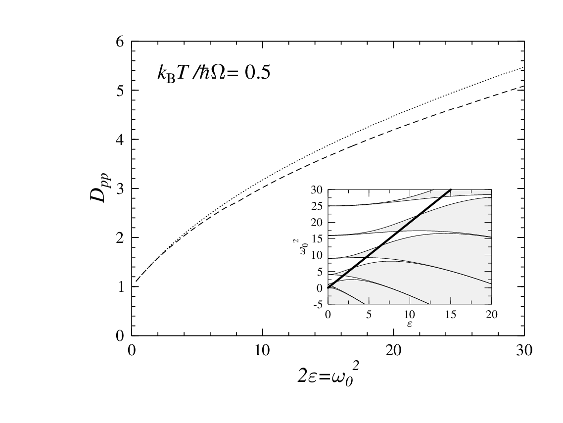
The influence of the quasienergies on the equation of motion (33) is given by different diffusion coefficients $D_{pp}$ . In Fig. 2, we compare the momentum-diffusion coefficients between the Markov approximation with respect to the unperturbed spectrum, given by Eq. (29), and the Markov approximation that relates to the quasienergy spectrum, given by Eq. (88). We have scaled the values to the classical momentum-diffusion coefficient $mk_{\rm B}T$ . The parameters $\omega_{0}^{2}$ and $\varepsilon$ are varied along the full line in the inset. Note that within the unstable regimes, perturbation theory is not valid. Nevertheless, Eq. (88) gives a smooth interpolation. The discrepances become most significant for strong driving and large $\omega_{0}^{2}$ . For both, low driving amplitude $\varepsilon\ll\omega_{0}^{2}$ and high temperature $T\gg\hbar\omega_{0}/k_{\rm B}$ , the difference vanishes.

The variances $\sigma_{xx}(t)$ and $\sigma_{pp}(t)$ of the Markov approximations without RWA are compared against the exact results [1] in the panels 3a and 3b. The chosen driving parameters $\omega^{2}=6.5\,\Omega^{2}$ and $\varepsilon=7\,\Omega^{2}$ lie inside the fifth stable zone ( $\mu=4.53513\,\Omega/2$ ). The temperature $k_{\rm B}T=0.5\,\hbar\Omega$ is sufficiently large, but with quantum effects still appreciable. We note that the improved Markov treatment in Sect. III.3.4, that accounts for the quasienergy differences, agrees better with the exact prediction. In the Figure we depict asymptotic times $\bar{t}>50$ , where transient effects have already decayed. The asymptotic co-variance elements retain the periodicity $\bar{T}=\pi$ of the external driving. For the chosen parameters the relative error is reduced by the use of the improved Markov scheme by approximately 30%.

The relative error $\eta_{xx}(t)=\sigma_{xx}^{\rm Markov}(t)/\sigma_{xx}^{\rm exact}(t)$ of the position variance for these two Markov approximations is depicted in panel 4. Note that the maximal deviations do not occur in the extrema, but happen to occur in the regions with negative slope.

As depicted with Fig. 5, the quality of both Markov approximations worsens with increasing dissipation strength $\gamma$ . This reflects the breakdown of the weak coupling approach when strong friction is ruling the system dynamics.

Results for the Markovian treatment within RWA, given in Sect. III.3.3, are depicted for the position variance $\sigma_{xx}(t)$ in Fig. 6. The driving parameters are the same as in Fig. 3. For this example, the quality of agreement to the exact result is similar for both Markov approximations. Nevertheless, the solution without RWA yields—up to a scale—a better overall agreement with the exact behaviour over a full driving period $T$ .

V Conclusion

We have used the parametrically driven harmonic oscillator as a simple working example to compare various versions of the Markovian approach to the quantum dynamics of periodically driven systems with dissipation, and to provide a synopsis of a number of alternative representations, each of which emphasizes different aspects of the same underlying physics.

The principal distinction to be made among possible Markovian approaches to the driven dissipative dynamics, refers to the degree to which changes in dynamical and spectral properties of the central system due to the driving are taken into account. In the crudest treatment, the non-unitary terms in the master equation are derived ignoring the explicit time dependence of the Hamiltonian, and the driving appears only in the unitary term. An improved master equation is obtained if the central system and the driving are coupled to the heat bath as one whole. The energy-domain quantity relevant for all subsequent developments is then the quasienergy spectrum, obtained within the Floquet formalism, instead of the unperturbed spectrum. In the time domain, the quantities entering the dissipative terms of the master equation, such as Heisenberg-picture operators of the central system, gain an explicit time dependence with the periodicity of the driving. As a bonus, the Floquet treatment of the central system with driving yields a well-adapted basis, the set of eigenstates of the Floquet operator. Representing the master equation in this basis completely removes the unitary term.

Besides the differences in representation, the use of the improved Floquet-Markov approximation in Sect. III.3.4 results mainly in a modified momentum diffusion that dependss on the quasienergy spectrum instead of the unperturbed spectrum of the central system. The difference becomes significant in the limits of strong driving amplitude and low temperature. An additive time-dependent external force, applied in addition to or instead of the parametric driving, undergoes a renormalization which vanishes, however, in the case of an Ohmic bath.

Even within the improved Markov approach, finer levels of approximation can be distinguished. A significant simplification of the master equation is achieved by a rotating-wave approximation, i.e. here, by neglecting reservoir-induced virtual transitions between Floquet states of the central system that violate quasienergy conservation. The resulting master equation has Lindblad form, with creation and annihilation operators acting on Floquet states, and thus manifestly generates a dynamical semigroup. This is not the case if the RWA is avoided. Apparently a drawback, the lack of a Lindblad structure in the master equation without RWA faithfully reflects the failure of the Markov approximation on short time scales.

An analogous situation as with the Lindblad form of the master equation arises with its Floquet structure. If all coefficients are at most periodically time dependent, then the equation of motion for the reduced density operator complies with the conditions for applicability of the Floquet theorem. As a consequence, the solutions can be cast in Floquet form, i.e., can be written as eigenfunctions of a generalized non-unitary Floquet operator that generates the evolution of the density operator over a single period. Since all variants of the Markov approximation discussed herein truncate the memory of the central system on time scales shorter than the period of the driving, the corresponding master equations have Floquet structure throughout. The exact path-integral solution, in contrast, allows for memory effects of unlimited duration and thereby generally prevents the consistent definition of a propagator over a single period.

Additional insight is gained by discussing the dynamics in terms of phase-space distributions, specifically, in terms of the Wigner representation of the density operator and its equation of motion. In this representation, the Floquet formalism is a useful device to construct and classify solutions. Since all Fokker-Planck equations obtained are time periodic, as are the corresponding master equations, their solutions may be written as eigenstates of a Wigner-Floquet operator (the Fokker-Planck operator evolving the Wigner function, integrated over a single period), or Wigner-Floquet states in short. They represent the quasiprobability distributions closest to the Floquet solutions of the corresponding classical Fokker-Planck equation.

Wigner-Floquet states with a purely real quasienergy correspond to asymptotic solutions. They are not literally stationary but retain the periodic time dependence of the driving. Since we are here dealing with a linear system, the asymptotic quasiprobability distributions follow the corresponding classical limit cycles. In the case of parametric driving, these limit cycles are trivial and correspond to a fixed point at the origin. A time dependence arises only by the periodic variation of the shape of the asymptotic distributions.

Concluding from a numerical comparison of certain dynamical quantities, for the specific case of the Mathieu oscillator, the attributes “simple” and “improved” for the two basic Markovian approaches prove adequate. Results for the Markov approximation based on the quasienergy spectrum show consistently better agreement with the exact path-integral solution than those for the Markov approximation with respect to the unperturbed spectrum. However, even in parameter regimes where the respective approximations are expected to become problematic, the differences in quality are not huge and the agreement with the exact solution is generally good. Technical advantages of the Markov approximation in general and of its various ramifications—easy analytical and numerical tractability, desirable formal properties such as Floquet or Lindblad form of the master equation—can justify to accept their quantitative inaccuracy.

Acknowledgments

Financal support of this work by the Deutsche Forschungsgemeinschaft (Grant No. Di 511/2-1 and Ha 1517/14-1) is gratefully achnowledged. We thank Christine Zerbe for providing us the numerical code for the path integral solution and Gert-Ludwig Ingold for helpful discussions.

Appendix A Solution of the Characteristic Equations

In this appendix, we solve the equation of motion for the Wigner function by the method of characteristics. For simplicity, we use here units with $m=1$ . We write $W(x,p,t)$ as

W(x,p,t)=\int{\rm d}X{\rm d}P\,{\rm e}^{{\rm i}xX+{\rm i}pP}{\rm e}^{S(X,P,t)}.

(99)

By this ansatz, equation (33) is transformed to the quasilinear partial differential equation

{\cal F}(X,S_{X},P,S_{P},t,S_{t})=0

(100)

for $S(X,P,t)$ , where ${\cal F}$ is given by

{\cal F}=S_{t}-XS_{P}+\gamma PS_{P}+k(t)PS_{X}+\gamma D_{pp}P^{2}+\gamma D_{xp}XP.

(101)

We denote the partial derivatives of $S(X,P,t)$ with respect to $X$ , $P$ and $t$ by $S_{X}$ , $S_{P}$ and $S_{t}$ , respectively.

The characteristic equations [26] of (100) are given by

$\displaystyle\dot{t}$	$\displaystyle=$	$\displaystyle\frac{\partial{\cal F}}{\partial S_{t}}=1,$	(102)
$\displaystyle\dot{X}$	$\displaystyle=$	$\displaystyle\frac{\partial{\cal F}}{\partial S_{X}}=k(t)P,$	(103)
$\displaystyle\dot{P}$	$\displaystyle=$	$\displaystyle\frac{\partial{\cal F}}{\partial S_{P}}=\gamma P-X,$	(104)
$\displaystyle\dot{S}_{X}$	$\displaystyle=$	$\displaystyle-\frac{\partial{\cal F}}{\partial X}=S_{P}-\gamma D_{xp}P,$	(105)
$\displaystyle\dot{S}_{P}$	$\displaystyle=$	$\displaystyle-\frac{\partial{\cal F}}{\partial P}=-\gamma S_{P}-k(t)S_{X}-2\gamma D_{pp}P-\gamma D_{xp}X,$	(106)
$\displaystyle\dot{S}_{t}$	$\displaystyle=$	$\displaystyle-\frac{\partial{\cal F}}{\partial t}=-\frac{{\rm d}k(t)}{{\rm d}t}PS_{X},$	(107)

whose solutions give the characteristics of the partial differential equation (100).

Equation (102) means that the characteristics can be parameterized by the time $t$ . Instead of equation (107), we will use (100) to get an expression for $S_{t}$ . So we only have to solve (103)–(106). The solutions of these equations can be traced back to the fundamental solutions $f_{i}(t)$ of the classical equation of motion (2).

From (103) and (104), we find

\ddot{P}-\gamma\dot{P}+k(t)P=0.

(108)

This is simply the classical equation of motion with a negative damping constant. Therefore the solutions for $X$ and $P$ read

	$\displaystyle P(t)$	$\displaystyle=$	$\displaystyle-c_{1+}{\rm e}^{\gamma t}f_{2}(t)+c_{2+}{\rm e}^{\gamma t}f_{1}(t),$		(109)
	$\displaystyle X(t)$	$\displaystyle=$	$\displaystyle c_{1+}{\rm e}^{\gamma t}\dot{f}_{2}(t)-c_{2+}{\rm e}^{\gamma t}\dot{f}_{1}(t),$		(110)

where $c_{i+}$ denote integration constants.

From (105) and (106) we find for $S_{X}$

\ddot{S}_{X}+\gamma\dot{S}_{X}+k(t)S_{X}=-2\gamma DP,

(111)

which is the classical equation of motion with an inhomogeneity. The effective diffusion constant $D$ is given by

D=D_{pp}+\gamma D_{xp}.

(112)

With the integration constants $c_{i-}$ , we integrate (111) with the Green function (9) to

S_{X}(t)=c_{1-}f_{1}(t)+c_{2-}f_{2}(t)-2\gamma D\int_{t_{0}}^{t}{\rm d}t^{\prime}\,G(t,t^{\prime})P(t^{\prime}),

(113)

and get by use of (105)

S_{P}(t)=c_{1-}\dot{f}_{1}(t)+c_{2-}\dot{f}_{2}(t)-2\gamma D\int_{t_{0}}^{t}{\rm d}t^{\prime}\,\frac{\partial G(t,t^{\prime})}{\partial t}P(t^{\prime})+\gamma D_{xp}P(t).

(114)

By inserting

P(t^{\prime})=G(t,t^{\prime})X(t)+\frac{\partial G(t,t^{\prime})}{\partial t}P(t),

(115)

obtained from Eqs. (109) and (110), we get a result for $S_{X}$ and $S_{P}$ that depends only on the endpoints of the characteristics. Now together with Eq. (100), we have an expression for ${\rm grad}\,S(X,P,t)=(S_{X},S_{P},S_{t})$ , which can be integrated to

	$\displaystyle S(X,P,t)$	$\displaystyle=$	$\displaystyle\Big(c_{1-}f_{1}(t)+c_{2-}f_{2}(t)\Big)X+\Big(c_{1-}\dot{f}_{1}(t)+c_{2-}\dot{f}_{2}(t)\Big)P$		(116)
			$\displaystyle-\frac{1}{2}\sigma_{xx}(t,t_{0})X^{2}-\sigma_{xp}(t,t_{0})XP-\frac{1}{2}\sigma_{pp}(t,t_{0})P^{2},$		(116)

with

$\displaystyle\sigma_{xx}(t,t_{0})$	$\displaystyle=$	$\displaystyle 2\gamma D\int_{t_{0}}^{t}{\rm d}t^{\prime}\left[G(t,t^{\prime})\right]^{2},$	(117)
$\displaystyle\sigma_{xp}(t,t_{0})$	$\displaystyle=$	$\displaystyle 2\gamma D\int_{t_{0}}^{t}{\rm d}t^{\prime}G(t,t^{\prime})\frac{\partial}{{\partial}t}G(t,t^{\prime}),$	(118)
$\displaystyle\sigma_{pp}(t,t_{0})$	$\displaystyle=$	$\displaystyle-\gamma D_{xp}+2\gamma D\int_{t_{0}}^{t}{\rm d}t^{\prime}\left[\frac{\partial}{{\partial}t}G(t,t^{\prime})\right]^{2}.$	(119)

By inserting $S(X,P,t)$ into (99), we find a solution for the Wigner function $W(x,p,t)$ .

The integration constants $c_{i\pm}$ are of course constant along the characteristics. Therefore the Poisson brackets between the expressions $c_{i\pm}(X,S_{X},P,S_{P},t)$ and ${\cal F}(X,S_{X},P,S_{P},t,S_{t})$ vanish [26]. By transforming back from Fourier space to real space, one finds that the operators $\hat{c}_{i\pm}\equiv c_{i\pm}(-{\rm i}\partial_{x},-{\rm i}x,-{\rm i}\partial_{p},-{\rm i}p,t)$ commute with the operator $\partial_{t}-L(t)$ , whose nullspace is the solution of the equation of motion. Therefore, the $\hat{c}_{i\pm}$ are shift operators in the subspace of solutions, i.e. if $W(x,p,t)$ is a solution of (33), then $\hat{c}_{i\pm}W(x,p,t)$ is also a solution.

For the $\hat{c}_{i\pm}$ we find

$\displaystyle\hat{c}_{1+}$	$\displaystyle=$	$\displaystyle\frac{1}{2}\left(f_{1}(t)\partial_{x}+\dot{f}_{1}(t)\partial_{p}\right),$	(120)
$\displaystyle\hat{c}_{2+}$	$\displaystyle=$	$\displaystyle\frac{1}{2}\left(f_{2}(t)\partial_{x}+\dot{f}_{2}(t)\partial_{p}\right)$	(121)
$\displaystyle\hat{c}_{1-}$	$\displaystyle=$	$\displaystyle{\rm i}\dot{f}_{2}(t)\Big(x+\sigma_{xx}(t,t_{0})\partial_{x}+\sigma_{xp}(t,t_{0})\partial_{p}\Big)$	(122)
		$\displaystyle-{\rm i}f_{2}(t)\Big(p+\sigma_{xp}(t,t_{0})\partial_{x}+\sigma_{pp}(t,t_{0})\partial_{p}\Big)$	(122)
$\displaystyle\hat{c}_{2-}$	$\displaystyle=$	$\displaystyle-{\rm i}\dot{f}_{1}(t)\Big(x+\sigma_{xx}(t,t_{0})\partial_{x}+\sigma_{xp}(t,t_{0})\partial_{p}\Big)$	(123)
		$\displaystyle+{\rm i}f_{1}(t)\Big(p+\sigma_{xp}(t,t_{0})\partial_{x}+\sigma_{pp}(t,t_{0})\partial_{p}\Big).$	(123)

Note that because of the linear structure of the characteristic equations, there is no ambiguity concerning the ordering of operators.

The operators $Q_{i+}(t)$ , used above, are proportional to the $\hat{c}_{i+}$ .

Appendix B The additively driven harmonic oscillator

In this appendix we present the Markovian master equation within the quasi-spectrum approach when the parametric oscillator is subjected to additional additive driving $-\hat{x}F(t)$ , i.e.

\hat{\cal H}(t)=\hat{H}_{\rm S}(t)-\hat{x}F(t).

(124)

With $\hat{H}_{\rm S}(t)$ being a time-independent harmonic oscillator, i.e., $k(t)=m\omega_{0}^{2}$ , the corresponding Markovian master equation in RWA for the dissipative system has already been given in [5]. Herein we generalize these results for the combined time-dependent system Hamiltonian in (124).

It is known that the only effect of the driving force $F(t)$ on the (quasi-) energy spectrum of a parametrically driven harmonic oscillator is an overall level shift [8]. Thus the level separations remain unaffected and we expect no change in the dissipative part of the master equation (27).

The classical equation of motion, which is also obeyed by the interaction-picture position operator, now reads

m\ddot{x}+k(t)x=F(t),

(125)

and can be integrated to yield the interaction-picture position operator

\tilde{x}(t,t^{\prime})=-\hat{x}\frac{\partial G^{0}(t,t^{\prime})}{\partial t^{\prime}}+\frac{\hat{p}}{m}G^{0}(t,t^{\prime})+\frac{1}{m}\int_{t^{\prime}}^{t}{\rm d}t^{\prime\prime}\,G^{0}(t,t^{\prime\prime})F(t^{\prime\prime}).

(126)

Thus we obtain a c-number correction to the interaction-picture position operator (82), given by the third term. After inserting (126) into (22), the generalized Markov approximation emerges as

	$\displaystyle\dot{\rho}_{\rm S}$	$\displaystyle=$	$\displaystyle\ldots+\frac{\rm i}{\hbar}F(t)\big[\hat{x},\rho_{\rm S}\big]$		(128)
			$\displaystyle-\frac{\rm i}{\hbar^{2}}\sum_{\nu}g_{\nu}^{2}\int_{0}^{\infty}{\rm d}\tau\,A_{\nu}(\tau)\big[\hat{x},\rho_{\rm S}\big]\frac{2}{m}\int_{t}^{t-\tau}{\rm d}t^{\prime}G^{0}(t-\tau,t^{\prime})F(t^{\prime}).$		(128)

The dots denote the old result for $F(t)=0$ , given by the right hand side of Eq. (27). The term in the first line stems from the reversible part of the master equation (22); the second one is a correction of the driving force due to the interaction with the bath. Thus the equation of motion for the density operator has the structure

\dot{\rho}_{\rm S}=\ldots+\frac{\rm i}{\hbar}\tilde{F}(t)\big[\hat{x},\rho_{\rm S}\big]

(129)

with an effective total driving force

\tilde{F}(t)=F(t)+\frac{2}{m\pi}\int_{0}^{\infty}{\rm d}\omega\,I(\omega)\int_{0}^{\infty}{\rm d}\tau\,\sin\omega\tau\int_{t}^{t-\tau}{\rm d}t^{\prime}G^{0}(t-\tau,t^{\prime})F(t^{\prime}).

(130)

Note that the dissipative parts of (129) are not affected by the additive driving force $F(t)$ . This makes explicit, that we must use a parametric time-dependence to study differences in the dissipative parts resulting from the Markov approximation with respect to the energy spectrum versus the Markov approximation with respect to the quasienergy spectrum.

With an Ohmic bath, $I(\omega)=m\gamma\omega$ , the integral in (130) vanishes and we obtain $\tilde{F}(t)=F(t)$ . Thus in contrast to an explicit parametric time dependence $k(t)$ in the quadratic part of the Hamiltonian, the time dependence of an additive force, in this case, does not change the Markovian master equation of the dissipative system.

References

[1] C. Zerbe and P. Hänggi, Phys. Rev. E 52, 1533 (1995).
[2] M. Grifoni, M. Sassetti, J. Stockburger, and U. Weiss, Phys. Rev. E 48, 3497 (1993); M. Grifoni, M. Sassetti, P. Hänggi, and U. Weiss, Phys. Rev. E 52, 3596 (1995).
[3] G. A. Voth, J. Phys. Chem. 97, 8365 (1993); D. E. Makarov and N. Makri, Phys. Rev. E 52, 5863 (1995).
[4] A. G. Fainshtein, N. L. Manakov, and L. P. Rapoport, J. Phys. B 11, 2561 (1978).
[5] R. Graham and R. Hübner, Ann. Phys. (NY) 234, 300 (1994).
[6] R. Blümel et al., Phys. Rev. A 44, 4521 (1991).
[7] T. Dittrich, B. Oelschlägel, and P. Hänggi, Europhys. Lett. 22, 5 (1993); B. Oelschlägel, T. Dittrich, and P. Hänggi, Acta Physica Polonica B 24, 845 (1993).
[8] V. S. Popov and A. M. Perelomov, Sov. Phys. JETP 30, 910 (1970).
[9] W. Magnus and S. Winkler, Hill’s Equation (Dover, New York, 1979); N. W. McLachlan, Theory and Applications of Mathieu Functions (Dover Publications, Inc., New York, 1964).
[10] R. Zwanzig, J. Stat. Phys. 9, 215 (1973).
[11] P. Hänggi, P. Talkner, and M. Borkovec, Rev. Mod. Phys. 62, 251 (1990); U. Weiss, Quantum Dissipative Systems, Vol. 2 of Series in Modern Condensed Matter Physics (World Scientific, Singapore, 1993).
[12] F. Haake, in Quantum Statistics in Optics and Solid-State Physics, Vol. 66 of Springer Tracts in Modern Physics, edited by G. Höhler (Springer, Berlin, 1973).
[13] R. Alicki and K. Lendi, in Quantum Dynamical Semigroups and Applications, Vol. 286 of Lecture Notes in Physics, edited by W. Beiglböck (Springer, Berlin, 1987).
[14] W. H. Louisell, Quantum Statistical Properties of Radiation (Wiley & Sons, New York, 1973).
[15] G. Lindblad, Commun. Math. Phys. 48, 119 (1976).
[16] P. Talkner, Ann. Phys (NY) 167, 390 (1986), see Appendix C therein.
[17] L. Diósi, Physica A 199, 517 (1993); L. Diósi, Europhys. Lett. 22, 1 (1993).
[18] P. Pechukas, Proc. NATO ASI “Large-Scale Molecular Systems” B258, 123 (1991).
[19] V. Ambegaokar, Berichte der Bunsengesellschaft 95, 400 (1991).
[20] I. Oppenheim and V. Romero-Rochin, Physica A 147, 184 (1987).
[21] I. M. Gradshteyn, I. S. Ryzhik, Table of Integrals, Series, and Products, 5th ed. (Academic Press, San Diego, 1994).
[22] H. Grabert, U. Weiss, and P. Talkner, Z. Phys. B 55, 87 (1984); P. Riseborough, P. Hänggi, and U. Weiss, Phys. Rev. A 31, 471 (1985); H. Grabert, P. Schramm, and G.-L. Ingold, Phys. Rep. 168, 115 (1988).
[23] E. Wigner, Phys. Rev. 40, 749 (1932); M. Hillery, R. F. O’Connell, M. Scully, and E. P. Wigner, Phys. Rep. 106, 121 (1984).
[24] H. Risken, The Fokker-Planck Equation, Vol. 18 of Springer Series in Synergetics (Springer, Berlin, 1984).
[25] P. Hänggi and H. Thomas, Phys. Rep. 88, 206 (1982).
[26] E. Kamke, Differentialgleichungen, 6 ed. (Teubner, Stuttgart, 1979), Vol. II. Partielle Differentialgleichungen.
[27] L. H’walisz, P. Jung, P. Hänggi, P. Talkner, and L. Schimansky-Geier, Z. Phys. B 77, 471 (1989).
[28] C. Zerbe, P. Jung, and P. Hänggi, Phys. Rev. E 49, 3626 (1994).
[29] U. M. Titulaer, Physica 91A, 321 (1978).
[30] V. S. Popov and A. M. Perelomov, Sov. Phys. JETP 29, 738 (1969).
[31] H. R. Lewis, Jr. and W. B. Riesenfeld, J. Math. Phys. 10, 1458 (1969).
[32] L. S. Brown, Phys. Rev. Lett. 66, 527 (1991).
[33] G. Schrade, V. I. Man’ko, W. P. Schleich, and R. J. Glauber, Quantum Semiclass. Opt. 7, 307 (1995).
[34] P. Jung and P. Hänggi, Phys. Rev. A 41, 2977 (1990); P. Jung, Phys. Rep. 234, 175 (1993).
[35] T.-S. Ho, K. Wang, and S.-I. Chu, Phys. Rev. A 33, 1798 (1986).
[36] W. Paul, Rev. Mod. Phys. 62, 531 (1990).

Refer to caption — Figure 1: Stability of equation (2) with $\gamma=0$ for the case of a Mathieu oscillator. In the white areas the Floquet index $\mu$ is real, which corresponds to stable solutions. In the shaded areas $\mu$ is complex and therefore one of the fundamental solutions (4) is unstable. On the borderlines $\mu$ becomes a multiple of $\Omega$ /2.