Self-homodyne tomography of a twin-beam state

The scheme of a self-homodyne detector is depicted in Fig. 1, along with the relevant modes of the electromagnetic field involved in the measurement. A nondegenerate optical parametric amplifier (NOPA) is injected with an input field having a strong coherent component at frequency $\omega_{0}$ with amplitudes $\alpha_{\updownarrow}$ and $\alpha_{\leftrightarrow}$ depending on the polarization, $\updownarrow$ denoting the vertical and $\leftrightarrow$ the horizontal polarization, respectively. The amplifier is pumped at the second harmonic $\omega_{p}=2\omega_{0}$ with amplitude $\alpha_{p}\gg\alpha_{\updownarrow},\alpha_{\leftrightarrow}$, such that the pump can be considered as classical and undepleted during the amplification process. At the output of the amplifier two photodetectors separately measure the intensities of a couple of orthogonally-polarized components of the field $\hat{\cal E}_{\updownarrow}$ and $\hat{\cal E}_{\leftrightarrow}$. At the output of the photodetectors, a narrow band of the photocurrent is selected, centered around frequency $\Omega\ll\omega_{0}$ (typically $\omega_{0}$ is optical/infrared, whereas $\Omega$ is a radio frequency). In the narrowband approximation and for radiation absorbed in a thin detector layer, the filtered output photocurrents are given by the (complex) operators

where $::$ denote the customary normal ordering with the (output) field annihilation-operator components $\hat{\cal E}^{+}_{\pi}$ on the right and the creation operators $\hat{\cal E}^{-}_{\pi}$ on the left, and the subindex $\pi$ runs on the two independent polarizations $\updownarrow$ and $\leftrightarrow$. In terms of the annihilation and creation operators $\hat{b}$ and $\hat{b}^{{\dagger}}$ of the relevant output modes one has

where the subindex $0$ refers to the central mode at frequency $\omega_{0}$, and $\pm$ refer to the sidebands at frequencies $\omega_{0}\pm\Omega$, respectively.

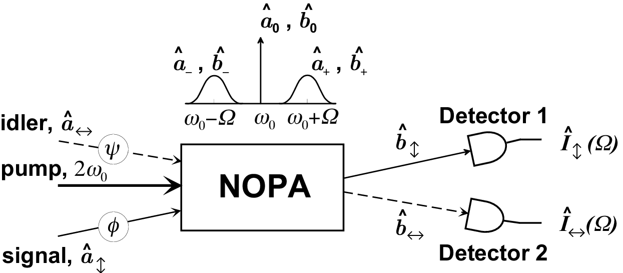
The input-output Heisenberg evolutions of the relevant field modes across the NOPA are given by

where $a$ and $a^{{\dagger}}$ denote the annihilation and creation operators for the input modes, $\mu=\cosh r$, $\nu=e^{i\theta_{p}}\sinh r$, $r\propto L\chi^{(2)}|\alpha_{p}|$ ($L$ is the amplifier length, $\chi^{(2)}$ is the effective second-order susceptibility). In the following we put $\theta_{p}=0$, namely we set the pump phase as the reference phase for all modes. We assume the mode $\hat{a}_{0\updownarrow}$ to be in a highly excited coherent state with amplitude $\alpha_{\updownarrow}$. For the purpose of measurement of the joint photon-number distribution, the mode $\hat{a}_{0\leftrightarrow}$ will also be assumed in a highly excited coherent state with amplitude $\alpha_{\leftrightarrow}$. In the case where we are interested in measuring the photon-number distribution of one beam only, the photocurrent produced by the ‘$\leftrightarrow$’-polarized beam can be ignored or the mode $\hat{a}_{0\leftrightarrow}$ can be assumed to be in the vacuum state. In the process of direct detection, the highly-excited central modes $\hat{a}_{0\updownarrow,\leftrightarrow}$ beat with the $\omega_{0}\pm\Omega$ sideband modes, thus playing the role of the LO of homodyne and heterodyne detectors. This converts the direct detectors into self-homodyne detectors whose experimental outcomes are the measured values of the following rescaled output photocurrents in the limit of strong LO’s:

where $\eta_{\updownarrow}$ and $\eta_{\leftrightarrow}$ denote the quantum efficiencies of the two photodetectors, $\alpha^{\ast}$ denotes the complex conjugate of $\alpha$, $\hat{\rho}_{\rm LO}$ represents the density operator of the LO state, and $\hbox{Tr}_{\rm LO}$ denotes the partial trace over the LO modes. In Eq. (4) $\hat{I}_{\pi}(\Omega)$ is modified from that in Eq. (2) because of the non-unity quantum efficiencies of the two photodetectors. It is given by

where $\hat{b}^{\prime}_{\gamma\pi}=\sqrt{\eta_{\pi}}\;\hat{b}_{\gamma\pi}+\sqrt{1-\eta_{\pi}}\;\hat{v}_{\gamma\pi}\;$. Here $\hat{v}_{\gamma\pi}$ for $\gamma\in\{0,+,-\}$ and $\pi\in\{\updownarrow,\leftrightarrow\}$ are independent vacuum-state operators accounting for the loss at the three frequency components of each polarization mode. For the sake of simplicity, we will assume $\eta_{\updownarrow}=\eta_{\leftrightarrow}=1$ for the rest of this Subsection. We will take into account the effect of non-unity quantum efficiency on the photocurrent probability distribution in Subsection II.2. Thus, using Eqs. (3) and quantum efficiency equal to unity, one obtains [25]

where $\phi=\mbox{arg}(\alpha_{\updownarrow}+\tau\alpha^{\ast}_{\leftrightarrow})$ is the phase of the mode $\hat{b}_{0\updownarrow}$ relative to that of the pump with $\tau=\tanh r$, and analogously $\psi=\mbox{arg}(\alpha_{\leftrightarrow}+\tau\alpha^{\ast}_{\updownarrow})$. Taking the real part of the photocurrents at given radio-frequency phases $\xi$ and $\chi$ one has

where the operator $\hat{X}_{\phi}(\hat{c})$ denotes the quadrature at phase $\phi$ of the mode with annihilation operator $\hat{c}$, namely,

and the operator $\hat{B}_{\pi}^{(\lambda)}$ is the annihilator of the polarized output mode

It is easy to check that the output modes (9) have corresponding input modes given by

and they are related by the Heisenberg evolutions

By scanning the relative phase $\phi$ between $\hat{b}_{0\updownarrow}$ and the pump mode, one can measure any quadrature $\hat{X}_{\phi}(\hat{B}_{\updownarrow}^{(\xi)})$ of the output field. If the input sideband modes $\hat{a}_{\pm}$ are in a state with a completely random phase, such as the vacuum, then the only phase reference in the output modes $\hat{b}_{\pm}$ is the pump phase $\theta_{p}=0$. In that case, the phase $\phi$ can be easily changed by delaying all the input fields with respect to the pump field, with no need to change the phase of $\hat{a}_{0\updownarrow}$ separately from the other input modes.

From Eq. (9) one can recognize that there are actually four output modes that commute with each other; hence, their quadratures could be jointly measured by the self-homodyne detectors. They are $\hat{B}_{\updownarrow}^{(\xi)}$, $\hat{B}_{\updownarrow}^{(\xi+\pi/2)}$, $\hat{B}_{\leftrightarrow}^{(\chi)}$, and $\hat{B}_{\leftrightarrow}^{(\chi+\pi/2)}$, corresponding to the “cosine” and “sine” components of the two photocurrents in Eqs. (6) at phases $\xi$ and $\chi$ respectively. The modes $\hat{B}^{(\lambda)}_{\updownarrow}$ and $\hat{B}^{(\lambda)}_{\leftrightarrow}$ are correlated due to the parametric interaction in Eq. (11). This interaction, however, does not couple the modes $\hat{B}^{(\lambda)}_{\updownarrow}$ and $\hat{B}^{(\lambda+\pi/2)}_{\leftrightarrow}$.

Since we are interested in using self-homodyne detection to measure the quadratures of two correlated modes $\hat{B}^{(\lambda)}_{\updownarrow}$ and $\hat{B}^{(\lambda)}_{\leftrightarrow}$, the radio-frequency phase $\lambda$ can always be set to zero by shifting the time origin. Then, the quadratures $\hat{X}_{\phi}(\hat{B}_{\updownarrow}^{(0)})$ and $\hat{X}_{\psi}(\hat{B}_{\leftrightarrow}^{(0)})$ are jointly measured. In the following we will use the shorthand notation $\hat{B}_{\pi}\equiv\hat{B}_{\pi}^{(0)}$ and $\hat{X}^{\pi}_{\phi}\equiv\hat{X}_{\phi}(\hat{B}_{\pi}^{(0)})$, and analogously for the input modes $\hat{A}_{\pi}\equiv\hat{A}_{\pi}^{(0)}$. For perfect detectors, the joint probability distribution of the “cosine” photocurrents with $\xi=\chi$ in Eqs. (7) coincides with the joint probability distribution of the two quadratures $\hat{X}^{\updownarrow}_{\phi}$ and $\hat{X}^{\leftrightarrow}_{\phi}$, namely,

where $|x,x^{\prime};\phi,\psi\rangle\doteq|x\rangle_{\phi}\otimes|x^{\prime}\rangle_{\psi}$ represents the simultaneous eigenvector of the two quadratures $\hat{X}^{\updownarrow}_{\phi}$ and $\hat{X}^{\leftrightarrow}_{\phi}$ with eigenvalues $x$ and $x^{\prime}$ in the Fock space ${\cal H}_{\updownarrow}\otimes{\cal H}_{\leftrightarrow}$ of the two modes $\hat{B}_{\updownarrow}$ and $\hat{B}_{\leftrightarrow}$, respectively; and $\hat{R}$ denotes their joint density operator. For detectors with non-unit quantum efficiencies $\eta_{\updownarrow}$ and $\eta_{\leftrightarrow}$, the joint probability distribution $p_{\eta_{\updownarrow}\eta_{\leftrightarrow}}(x,x^{\prime};\phi,\psi)$ of the photocurrents is the convolution [25] of the ideal probability in Eq. (12) with Gaussians for each mode of variances

In this way, the resulting output probability distribution can be written in the form

For simplicity, in the following we will assume equal quantum efficiencies $\eta_{\updownarrow}=\eta_{\leftrightarrow}\equiv\eta$ for both detectors. Notice that in the limit of unit quantum efficiency, $\eta\to 1$, one has $\Delta_{\eta}\to 0$, and the ideal probability in (12) is recovered.

We are now interested in the simplest case of measurement, that with $\omega_{0}\pm\Omega$ sidebands in the vacuum state at the input of the NOPA (i.e., parametric fluorescence). In the Schrödinger picture, Eqs. (11) correspond to the following state generated at the output of the NOPA:

where $\tau=\tanh r$, and the two-mode Fock state $|n,m\rangle$ pertaining to $\hat{B}_{\updownarrow}$ and $\hat{B}_{\leftrightarrow}$ is given by

where $|0,0\rangle$ denotes the vacuum for both the $\hat{B}_{\pi}$ modes. For the state (15) the photon-number probability is given by

where

is the average number of photons in each mode at the NOPA output due to parametric fluorescence. The main feature of the distribution (17) is the perfect correlation of the photon numbers in the signal and idler modes. The two-mode photon-number probability $p(n,m)$ of Eq. (17) is shown in Fig. 2(left).

The joint probability distribution of the output photocurrents is derived in the Appendix, and is given by

which can also be cast in the equivalent form

where

In the case that we measure only a single output photocurrent, say $\hat{}\char 16\relax_{\updownarrow}(\Omega)$—namely, we ignore the measured value of the other photocurrent $\hat{}\char 16\relax_{\leftrightarrow}(\Omega)$—the self-homodyne detector is equivalent to a conventional homodyne detector, which measures only the quadrature $\hat{X}^{\updownarrow}_{\phi}$ of mode $\hat{B}_{\updownarrow}$. The output probability distribution is given by

where the reduced density operator of the mode $\hat{B}_{\updownarrow}$ is

with $\hbox{Tr}_{\leftrightarrow}$ denoting the partial trace over the Hilbert space of the undetected mode $\hat{B}_{\leftrightarrow}$. The reduced density operator of the mode $\hat{B}_{\updownarrow}$ in Eq. (23) is that of a thermal state with the photon-number probability

where the average photon number $\bar{n}$ is given by Eq. (18). The probability distribution of the output photocurrent, Eq. (22), is a Gaussian with variance $\Delta^{2}={1\over 2}(\bar{n}+{1\over 2})+\Delta^{2}_{\eta}$, centered at zero. This result of self-homodyning of only the signal mode has been recently demonstrated experimentally [24].

Let us note that, while our analysis is aimed at the measurement of the joint signal-idler photon distribution, a similar self-homodyning approach can also be implemented to measure the joint distribution of $\pm 45^{\circ}$-polarized OPA outputs. In that case, a quadrature of the annihilation operator

is detected at a phase arg$(\alpha_{\pi}+\tau\alpha^{\ast}_{\pi})$, where the subindex $\pi$ runs on the two independent $\pm 45^{\circ}$ polarizations, namely $\nearrow$ and $\nwarrow$, and $\alpha_{\pi}$ is the coherent-state amplitude of the corresponding central-frequency component of the input. Since the interaction (25) does not couple the $+45^{\circ}$ and $-45^{\circ}$ modes with each other, the polarization non-degenerate OPA is equivalent to two degenerate OPA’s. Two-mode joint photon-number distribution is just a product of the marginal distributions for each mode, and in the case of vacuum-state input sidebands is given by [18]

where the mean photon number $\bar{n}$ in each mode is given by Eq. (18). The probability distribution (26) is shown in Fig. 2(right), next to the signal-idler joint photon-number distribution of Eq. (17). While the $\pm 45^{\circ}$ modes exhibit independent photon-number oscillations in Fig. 2(right), the signal and idler correlations in Fig. 2(left) result in oscillations of the total photon number.

The method for reconstructing the matrix elements of the density operator is based on the following resolution of the identity on the Hilbert-Schmidt space

where the integral is extended to the complex plane ${\bf C}$ for $w$, and $\hat{D}(w)=\exp(-w^{\ast}\hat{a}+w\hat{a}^{\dagger})$ denotes the displacement operator for the field mode of interest with annihilation operator $\hat{a}$. Equation (27) simply follows from the orthogonality relation for displacement operators

where $\delta_{2}(w)$ denotes the Dirac delta-function on the complex plane. By changing to polar variables $w=(i/2)ke^{i\phi}$, Eq. (27) becomes

where $\hat{X}_{\phi}=\frac{1}{2}\left(\hat{a}^{\dagger}e^{i\phi}+\hat{a}e^{-i\phi}\right)$ denotes the quadrature operator for the field mode $\hat{a}$. Then we evaluate the trace using the eigenvectors $\{|x\rangle_{\phi}\}$ of $\hat{X}_{\phi}$, and multiply and divide the function inside the integral by $\exp[(1-\eta)k^{2}/(8\eta)]$ in the following fashion:

where $p(x,\phi)={}_{\phi}\langle x|\hat{\varrho}|x\rangle_{\phi}$ is the ideal homodyne probability. Using the convolution theorem we obtain

where $p_{\eta}(x;\phi)$ is the homodyne probability distribution for non-unit quantum efficiency $\eta$, which is the convolution of $p(x,\phi)$ with a Gaussian of variance $\Delta^{2}_{\eta}$ given in Eq. (13). The kernel $\hat{K}_{\eta}(x-\hat{X}_{\phi})$ in Eq. (31) is formally given by

where convergence of the integral in Eq. (32) for the operator $\hat{K}_{\eta}(x-\hat{X}_{\phi})$ is intended in the weak sense of convergence of the matrix elements $\langle\upsilon|\hat{K}_{\eta}(x-\hat{X}_{\phi})|\upsilon^{\prime}\rangle$ between the Hilbert-space vectors $|\upsilon\rangle$ and $|\upsilon^{\prime}\rangle$, which are evaluated before integration. From Eq. (31) it follows that the matrix element $\langle\upsilon|\hat{\varrho}|\upsilon^{\prime}\rangle$ can be experimentally obtained by averaging the function $\langle\upsilon|\hat{K}_{\eta}(x-\hat{X}_{\phi})|\upsilon^{\prime}\rangle$ over the quadrature outcomes $x$ that are homodyne detected at random phases $\phi$ with respect to the LO, namely,

where the overbar denotes the experimental average. The functions $\langle\upsilon|\hat{K}_{\eta}(x-\hat{X}_{\phi})|\upsilon^{\prime}\rangle$ for different vectors $|\upsilon\rangle$ and $|\upsilon^{\prime}\rangle$ are called “pattern-functions” after Ref. [6].

In Ref. [5] the boundness of different types of matrix elements of the operator kernel $\hat{K}_{\eta}(x-\hat{X}_{\phi})$ was analyzed as a function of the quantum efficiency. It was shown that for the photon-number and coherent-state representations these matrix elements become unbounded for $\eta\leq 1/2$. The fact that $\eta=1/2$ is a lower bound for measuring the state in any (not exotic) representation was thoroughly discussed in Ref. [8]. The way in which nonunit quantum efficiency manifests its detrimental effect when approaching the lower bound is through increasingly large statistical errors. Let us restrict our attention to the photon-number representation. At $\eta=1$, as proven in Ref. [26], the statistical errors of the diagonal matrix elements $\langle n|\hat{\varrho}|n\rangle$ saturate at the limiting value $\sqrt{2/N}$ for sufficiently large $n$, independently of the state $\hat{\varrho}$ ($N$ is the number of data collected in the experiment). Also, errors of the off-diagonal elements increase very slowly versus the distance from the main diagonal. On the other hand, for $\eta<1$ the errors increase dramatically versus either $n$ or $1-\eta$, and eventually become infinite at the lower bound $\eta=1/2$ [27]. In the next section we will see how this behavior manifests itself in the two-mode tomography measurement, on the basis of numerical results from Monte-Carlo simulation experiments.

It is easy to see that Eq. (27) can be extended because of linearity to the case of $M$ modes as follows:

where $\hat{R}$ now denotes the joint $M$-mode density operator, and $\hat{D}_{l}(w_{l})$ is the displacement operator for the $l$-th mode. As a consequence, Eq. (33) is extended to the multimode measurement in the following way:

where $|\Phi\rangle$ and $|\Phi^{\prime}\rangle$ are now multimode vectors, and the experimental average is taken over the random outcomes $x_{l}$ of the joint homodyne measurement of quadratures $\hat{X}^{(l)}_{\phi_{l}}$, $l=1,...,M$, of all $M$ modes with random LO phases $\phi_{l}$ (we have also let the quantum efficiency to be different for each homodyne detector). Equation (35) agrees with the results obtained in Refs. [19].

As we have seen in Section II, in the self-homodyne measurement one can jointly measure the quadratures $\hat{X}^{\updownarrow}_{\phi}$ and $\hat{X}^{\leftrightarrow}_{\psi}$ of two different modes $\hat{B}_{\updownarrow}$ and $\hat{B}_{\leftrightarrow}$, and thus, in principle, perform a two-mode tomography of the OPA output. However, in order to perform two-mode tomography we need uncorrelated phases $\phi$ and $\psi$ for the quadratures, whereas in the self-homodyne measurement they are actually correlated. In fact, one has

In the case when we are interested in the photon distribution of one mode only, we can assume $\alpha_{\leftrightarrow}=0$. Then, by letting the phase of $\alpha_{\updownarrow}$ fluctuate with a uniform distribution from $0$ to $2\pi$, one can perform one-mode tomography of Eq. (33). On the other hand, if we are interested in the joint photon-number distribution, then we can not make the measurement by simply averaging the two-mode pattern functions over the experimental outcomes as in Eq. (35). This is because the LO phases $\phi$ and $\psi$ in this case are not independent random variables. We will show, however, that it is possible to take the correlation of $\phi$ and $\psi$ into account and still perform two-mode tomography by appropriately weighting the experimental outcomes in Eq. (35). We first rewrite Eq. (35) in the two-mode case as follows:

We focus our attention on the phase average only. For LO’s with equal intensities $|\alpha_{\leftrightarrow}|=|\alpha_{\updownarrow}|$ and phases $\varphi_{\updownarrow}=\mbox{arg}(\alpha_{\updownarrow})$ and $\varphi_{\leftrightarrow}=\mbox{arg}(\alpha_{\leftrightarrow})$, one has

After performing the change of variables

the average over the phases can be rewritten in terms of the average over the sum and difference phases with an appropriate weighting function as follows:

where the weighting function is given by

Since the input phases $\varphi_{\updownarrow}$ and $\varphi_{\leftrightarrow}$ can certainly be considered as random and uncorrelated, the same must hold true for their half-sum $\sigma$ and half-difference $\delta$ in Eq. (39). Then, the measurement of the matrix element in Eq. (37) is obtained by averaging over the experimental random phases $\sigma$ and $\delta$ with the weighting function (41). Also, the weighting function can be rewritten in terms of the gain $g(\sigma)$ of the central-frequency component that is given by

Hence, the weighting function is simply

which can be easily and independently measured for every data point while the homodyne data are collected.

This approach to phase averaging can also be used for detection of the $\pm 45^{\circ}$ modes mentioned in Subsection II.2. In that case, the quadrature phases arg$(\alpha_{\nearrow}+\tau\alpha^{\ast}_{\nearrow})$ and arg$(\alpha_{\nwarrow}+\tau\alpha^{\ast}_{\nwarrow})$ are independent, but non-uniformly distributed. Then, the averaging is done over the input phase $\sigma={\rm arg}(\alpha_{\nearrow})$ or $\sigma={\rm arg}(\alpha_{\nwarrow})$, respectively, with the weighting function (43) given by the phase-sensitive gain of the central component.

For non-unit quantum efficiency one can measure the density matrix elements for $\eta$ above the bound $\eta=1/2$. However, instead of measuring the density matrix of the state $\hat{R}$ of interest, one can always measure the density matrix of the state that has been damped—or “dressed”—by the quantum efficiency, without any limitation for $\eta$, even though such a dressed state would be less and less significant for lower quantum efficiencies. The concepts of “dressed” and “bare” states are two faces of the same measurement description when regarded in the equivalent Schrödinger and Heisenberg pictures. The conventional description corresponds to the Heisenberg picture, in which the true state—also called the “signal” or the “bare” state—is measured and the effect of quantum efficiency is ascribed to the detector observable (photocurrent). In the “dressed” state description, on the other hand, one regards the measurement with $\eta<1$ on the true state $\hat{R}$ as the corresponding hypothetical “bare measurement” with $\eta=1$, but now on the “dressed” state $\hat{R}_{\eta}$, ascribing the effect of the non-unit quantum efficiency to the quantum state itself, rather than to the detector. In other words, the effect of the non-unit quantum efficiency is regarded in a Schrödinger-like picture, with the state evolving from $\hat{R}$ to $\hat{R}_{\eta}$, where the quantum efficiency plays the role of a time parameter.

An easy way to perform tomographic measurement on a dressed state is just to use the experimental data for $\eta<1$ and analyze them using the pattern function with $\eta=1$. As shown in Subsection II.2, the effect of non-unit quantum efficiency is to convolve the quadrature-probability distributions for all LO phases with a Gaussian of variance $\Delta^{2}_{\eta}$ given by Eq. (13). This corresponds to convolving the Wigner function with an isotropic Gaussian of the same variance $\Delta^{2}_{\eta}$ in the complex plane, which, in turn, corresponds to adding Gaussian noise to the quantum state. In terms of the bare state $\hat{\varrho}$, the state $\hat{\Gamma}_{\eta}(\hat{\varrho})$ dressed with the Gaussian noise is given by [28]

where the noise-equivalent mean thermal photon number $\bar{m}$ is related to the quantum efficiency through

In the multimode case, one needs to apply the transformation (44) repeatedly, once per each mode, with the corresponding displacement operator of the mode. In the context of measuring the bare state, Eq. (44) was exploited in Ref. [29] to show that the measurement is possible even in the presence of quantum noise, however, with no more than $\bar{m}=1/2$ thermal photons.

Another way of dressing the state, which is often employed in experimental analysis of the tomographic data (see Refs. [11, 12, 24]) is to consider the state that has undergone a loss equivalent to $\eta$. In this case, the analysis is done by rescaling the output photocurrents by $\sqrt{\eta}$ instead of $\eta$ as in Eqs. (4), and then using the pattern functions for $\eta=1$. It is easy to see that this procedure corresponds to measuring the dressed state $\hat{\Lambda}_{\eta}(\hat{\varrho})$, which is related to the bare state $\hat{\rho}$ as follows:

Again, in the multimode case the transformation (46) is applied separately to all modes. One can also regard the state $\hat{\Lambda}_{\eta}(\hat{\varrho})$ in Eq. (46) as the state of the mode $\sqrt{\eta}\;\hat{a}+\sqrt{1-\eta}\;\hat{v}$—instead of the state of just the mode $\hat{a}$ of interest—where $\hat{v}$ is the independent vacuum-state mode responsible for the loss.

Before concluding this section, we need to say a few words regarding the difference between the two dressed states $\hat{\Lambda}_{\eta}(\hat{\varrho})$ and $\hat{\Gamma}_{\eta}(\hat{\varrho})$. In the loss model corresponding to $\hat{\Lambda}_{\eta}(\hat{\varrho})$, the dressed state loses some signal, and becomes the vacuum state in the limit of $\eta\to 0$, independently of $\hat{\varrho}$, which makes the state less and less meaningful for decreasing $\eta$. On the other hand, in the Gaussian-noise model corresponding to $\hat{\Gamma}_{\eta}(\hat{\varrho})$, there is no loss of signal, but the state gets an increasingly large number of thermal photons for decreasing $\eta$. In this way, the most interesting quantum features of the state—as, for example, oscillations in the photon-number probability—are lost, as shown in Ref. [5], and all states tend to look “classical”. In the next section we will see these effects at work in some Monte-Carlo numerical experiments for the two-mode case.