Statistical uncertainty in quantum optical photodetection measurements

Konrad Banaszek Address: Instytut Fizyki Teoretycznej, Uniwersytet Warszawski, Hoża 69, PL-00-681 Warszawa, Poland

August 11, 2026

Abstract

We present a complete statistical analysis of quantum optical measurement schemes based on photodetection. Statistical distributions of quantum observables determined from a finite number of experimental runs are characterized with the help of the generating function, which we derive using the exact statistical description of raw experimental outcomes. We use the developed formalism to point out that the statistical uncertainty results in substantial limitations of the determined information on the quantum state: though a family of observables characterizing the quantum state can be safely evaluated from experimental data, its further use to obtain the expectation value of some operators generates exploding statistical errors. These issues are discussed using the example of phase–insensitive measurements of a single light mode. We study reconstruction of the photon number distribution from photon counting and random phase homodyne detection. We show that utilization of the reconstructed distribution to evaluate a simple well–behaved observable, namely the parity operator, encounters difficulties due to accumulation of statistical errors. As the parity operator yields the Wigner function at the phase space origin, this example also demonstrates that transformation between various experimentally determined representations of the quantum state is a quite delicate matter.

pacs

PACS Number(s): 42.50.Dv, 42.50.Ar, 03.65.Bz

I Introduction

Over recent years, the set of tools for measuring quantum statistical properties of optical radiation has substantially enlarged. The experimental demonstration of optical homodyne tomography [1] has been followed by detailed studies of this beautiful technique [2, 3, 4, 5, 6, 7, 8], and diverse novel schemes have been proposed [9, 10, 11, 12, 13, 14]. The quantum optical “toolbox” for measuring light contains now experimentally established schemes for reconstructing various representations of its quantum state: the $Q$ function [15], the Wigner function, and the density matrix in the quadrature and the Fock bases [1, 2, 3]. A device that is used in most of quantum optical schemes to convert the quantum signal to a macroscopic level is the photodetector. Thus, photodetection is a basic ingredient of quantum optical measurements.

The quantum state can be characterized using various representations: quasidistribution functions or a density matrix in a specific basis. From a theoretical point of view, all these forms are equivalent. Each representation contains complete information on the quantum state, and they can be transformed from one to another. Any observable related to the measured systems can be evaluated from an arbitrary representation using an appropriate expression.

This simple picture becomes much more complicated when we deal with real experimental data rather than analytical formulae. Each quantity determined from a finite number of experimental runs is affected by a statistical error. Consequently, the density matrix or the quasidistribution function reconstructed from the experimental data is known only with some statistical uncertainty. This uncertainty is important when we further use the reconstructed information to calculate other observables or to pass to another representation. The crucial question is, whether determination of a certain representation with sufficient accuracy guarantees that arbitrary observable can be calculated from these data with a reasonably low statistical error. If this is not the case, the reconstructed information on the quantum state of the measured system turns out to be somewhat incomplete. Furthermore, transformation between various representations of the quantum state becomes a delicate matter.

These and related problems call for a rigorous statistical analysis of quantum optical measurements. The purpose of this paper is to provide a complete statistical description of a measurement of quantum observables in optical schemes based on photodetection. This approach fully characterizes statistical properties of quantities determined in a realistic measurement from a finite number of experimental runs. It can be applied either to determination of a single quantum observable, or to the reconstruction of the quantum state in a specific representation. Within the presented framework we study, using a simple example, the completeness of the experimentally reconstructed information on the quantum state. We demonstrate the pathological behavior suggested above, when the reconstructed data cannot be used to calculate some observables due to rapidly exploding statistical errors.

An important issue is the statistical methodology applied to retrieve information on the measured quantum system from experimental data. Various approaches have been recently developed, based on the maximum entropy principle [16], the least–squares inversion [17], and the maximum likelihood estimation [18, 19]. In this paper we will consider the most straightforward and so far the most commonly used strategy, where experimental relative frequencies are taken as estimates for quantum mechanical probability distributions. Quantum observables are reconstructed from these data via linear transformations.

Selected aspects of statistical uncertainty resulting from the finite character of the experimental data sample have been discussed in some particular cases. Systematic and statistical errors in homodyne measurements of the density matrix were studied [5, 6], and it was found that homodyne detection of quantum observables is accompanied by excess noise compared to a direct measurement [7]. Analysis of a photon counting scheme for sampling quantum phase space showed that compensation for the nonunit detection efficiency is in general not possible [20]. The present paper provides a general statistical analysis of quantum optical schemes based on photodetection.

This paper is organized as follows. The starting point of our analysis is the probability distribution of obtaining a specific histogram from $N$ runs of the experimental setup. This basic quantity determines all statistical properties of quantum observables reconstructed from a finite sample of experimental data. We characterize these properties using the generating function, for which we derive an exact expression directly from the probability distribution of the experimental outcomes. These general results are presented in Sec. II. Then, in Sec. III, we use the developed formalism to discuss the reconstruction of the photon number distribution of a single light mode, and its subsequent utilization to evaluate the parity operator $\hat{\Pi}$ . We consider two experimental schemes: direct photon counting using an imperfect detector, and homodyne detection with random phase. In both the cases we find that the evaluation of the parity operator from the reconstructed photon statistics is a very delicate matter. For photon counting of a thermal state, we show that neither the statistical mean value of $\hat{\Pi}$ nor its variance have to exist when we take into account arbitrarily high count numbers. For random phase homodyne detection, the statistical error of the parity operator is an interplay of the number of runs $N$ and the specific regularization method used for its evaluation. The example of the parity operator illustrates difficulties related to the transformations between various experimentally determined representations of the quantum state, as the parity operator yields, up to a multiplicative constant, the Wigner function at the phase space origin. Finally, Sec. IV summarizes the paper.

II Statistical analysis of experiment

In photodetection measurements, the raw quantity delivered by a single experimental run is the number of photoelectrons ejected from the active material of the detectors. The data recorded for further processing depends on a specific scheme. It may be just the number of counts on a single detector, or a difference of photocounts on a pair of photodetectors, which is the case of balanced homodyne detection. It may also be a finite sequence of integer numbers, e.g. for double homodyne detection. We will denote in general this data by $n$ , keeping in mind all the possibilities.

The experimental scheme may have some external parameters $\theta$ , for example the phase of the local oscillator in homodyne detection. The series of measurements are repeated for various settings $\theta_{i}$ of these parameters. Thus, what is eventually obtained from the experiment, is a set of histograms $\{k_{n}\}_{\theta_{i}}$ , telling in how many runs with the settings $\theta_{i}$ the outcome $n$ has been recorded. We assume that for each setting the same total number of $N$ runs has been performed.

The theoretical probability $p_{n}(\theta_{i})$ of obtaining the outcome $n$ in a run with settings $\theta_{i}$ is given by the expectation value of a positive operator valued measure (POVM) $\hat{p}_{n}(\theta_{i})$ acting in the Hilbert space of the measured system. The reconstruction of an observable $\hat{A}$ is possible, if it can be represented as a linear combination of the POVMs for the settings used in the experiment:

\hat{A}=\sum_{i}\sum_{n}a_{n}(\theta_{i})\hat{p}_{n}(\theta_{i}),

(1)

where $a_{n}(\theta_{i})$ are the kernel functions. The above formula allows one to compute the quantum expectation value $\langle\hat{A}\rangle$ from the probability distributions $p_{n}(\theta_{i})$ .

This theoretical relation has to be applied now to the experimental data. The simplest and the most commonly used strategy is to estimate the probability distributions $p_{n}(\theta_{i})$ by experimental relative frequencies $(k_{n}/N)_{\theta_{i}}$ . The relative frequencies integrated with the appropriate kernel functions yield an estimate for the expectation value of the operator $\hat{A}$ . For simplicity, we will denote this estimate just by $A$ . Thus, the recipe for reconstructing the observable $A$ from experimental data is given by the counterpart of Eq. (1):

A=\sum_{i}\sum_{n}a_{n}(\theta_{i})\left(\frac{k_{n}}{N}\right)_{\theta_{i}}.

(2)

We will now analyse statistical properties of the observable $A$ evaluated according to Eq. (2) from data collected in a finite number of experimental runs. Our goal is to characterize the statistical distribution $w(A)$ defining the probability that the experiment yields a specific result $A$ . The fundamental object in this analysis is the probability ${\cal P}(\{k_{n}\};\theta)$ of obtaining a specific histogram $\{k_{n}\}$ for the settings $\theta$ . In order to avoid convergence problems, we will restrict the possible values of $n$ to a finite set by introducing a cut–off. The probability ${\cal P}(\{k_{n}\};\theta)$ is then given by the multinomial distribution:

{\cal P}(\{k_{n}\};\theta)=\frac{N!}{(N-\sum_{n}^{\prime}k_{n})!}\left(1-{\sum_{n}}^{\prime}p_{n}(\theta)\right)^{N-\sum_{n}^{\prime}k_{n}}{\prod_{n}}^{\prime}\frac{1}{k_{n}!}[p_{n}(\theta)]^{k_{n}},

(3)

where prim in sums and products denotes the cut–off.

Let us first consider a contribution $A_{i}$ to the observable $A$ calculated from the histogram $\theta_{i}$ :

A_{i}={\sum_{n}}^{\prime}a_{n}(\theta_{i})\left(\frac{k_{n}}{N}\right)_{\theta_{i}}.

(4)

Its statistical distribution $w(A_{i};\theta_{i})$ is given by the following sum over all possible histograms that can be obtained from $N$ experimental runs:

w(A_{i};\theta_{i})=\sum_{\{k_{n}\}}{\cal P}(\{k_{n}\};\theta_{i})\delta\left(A_{i}-\frac{1}{N}{\sum_{n}}^{\prime}a_{n}(\theta_{i})k_{n}\right).

(5)

Equivalently, the statistics of $A_{i}$ can be characterized by the generating function $\tilde{w}(\lambda;\theta_{i})$ for the moments, which is the Fourier transform of the distribution $w(A_{i};\theta_{i})$ :

	$\displaystyle\tilde{w}(\lambda;\theta_{i})$	$\displaystyle=$	$\displaystyle\int\text{d}A_{i}\;e^{i\lambda A_{i}}w(A_{i};\theta_{i})$		(6)
		$\displaystyle=$	$\displaystyle\sum_{\{k_{n}\}}{\cal P}(\{k_{n}\};\theta_{i})\exp\left(\frac{i\lambda}{N}{\sum_{n}}^{\prime}a_{n}(\theta_{i})k_{n}\right).$		(6)

An easy calculation yields the explicit form of the generating function:

\tilde{w}(\lambda;\theta_{i})=\left(1+{\sum_{n}}^{\prime}p_{n}(\theta_{i})(e^{i\lambda a_{n}(\theta_{i})/N}-1)\right)^{N}.

(7)

The observable $A$ is obtained via summation of the components $A_{i}$ corresponding to all settings of the external parameters $\theta_{i}$ . As these components are determined from disjoint subsets of the experimental data, they are statistically independent. Consequently, the generating function $\tilde{w}(\lambda)$ for the moments of the observable $A$ is given by the product:

	$\displaystyle\tilde{w}(\lambda)$	$\displaystyle=$	$\displaystyle\int\text{d}A\;e^{i\lambda A}w(A)=\prod_{i}\tilde{w}(\lambda;\theta_{i})$		(8)
		$\displaystyle=$	$\displaystyle\prod_{i}\left(1+{\sum_{n}}^{\prime}p_{n}(\theta_{i})(e^{i\lambda a_{n}(\theta_{i})/N}-1)\right)^{N}.$		(8)

This expression contains the complete statistical information on determination of the observable $A$ from a finite number of runs of a specific experimental setup. The measuring apparatus is included in this expression in the form of a family of POVMs $\hat{p}_{n}(\theta_{i})$ . The quantum expectation value of these POVMs over the state of the measured system yields the probability distributions $p_{n}(\theta_{i})$ . Finally, the coefficients $a_{n}(\theta_{i})$ are given by the computational recipe for reconstructing the observable $A$ from the measured distributions.

The basic characteristics of statistical properties of the observable $A$ is provided by the mean value $\text{E}(A)$ and the variance $\text{Var}(A)$ . These two quantities can be easily found by differentiating the logarithm of the generating operator:

$\displaystyle\text{E}(A)$	$\displaystyle=$	$\displaystyle\left.\frac{1}{i}\frac{\text{d}}{\text{d}\lambda}\log\tilde{w}(\lambda)\right\|_{\lambda=0}=\sum_{i}{\sum_{n}}^{\prime}a_{n}(\theta_{i})p_{n}(\theta_{i}),$	(9)
$\displaystyle\text{Var}(A)$	$\displaystyle=$	$\displaystyle\left.\frac{1}{i^{2}}\frac{\text{d}^{2}}{\text{d}\lambda^{2}}\log\tilde{w}(\lambda)\right\|_{\lambda=0}$	(10)
	$\displaystyle=$	$\displaystyle\frac{1}{N}\left[\sum_{i}{\sum_{n}}^{\prime}a_{n}^{2}(\theta_{i})p_{n}(\theta_{i})-\sum_{i}\left({\sum_{n}}^{\prime}a_{n}(\theta_{i})p_{n}(\theta_{i})\right)^{2}\right].$	(10)

The statistical error is scaled with the inverse of the square root of the number of runs $N$ . Let us note that the second component in the derived formula for $\text{Var}(A)$ differs from that used in the discussions of homodyne tomography in Refs. [6, 7], where it was equal just to $[\text{E}(A)]^{2}$ . This difference results from different assumptions about the local oscillator phase: in Refs. [6, 7] it was considered to be a stochastic variable in order to avoid systematic errors, whereas we have assumed that the number of runs is fixed for each selected setting of the external parameters.

The goal of quantum state measurements is to retrieve the maximum amount of information on the quantum state available from the experimental data. Therefore the experimental histograms are usually processed many times in order to reconstruct a family of observables characterizing the quantum state. Of course, quantities determined from the same set of experimental data are not statistically independent, but in general may exhibit correlations. The analysis presented above can be easily extended to evaluation of any number of observables from the experimental data. If we restrict our attention to the basic, second–order characterization of these correlations, it is sufficient to discuss determination of two observables. Let us suppose that in addition to $A$ , another observable $B$ has been calculated from the histograms $\{k_{n}\}_{\theta_{i}}$ according to the formula:

B=\sum_{i}{\sum_{n}}^{\prime}b_{n}(\theta_{i})\left(\frac{k_{n}}{N}\right)_{\theta_{i}}.

(11)

The generating function $\tilde{w}(\lambda,\mu)$ corresponding to the joint probability distribution $w(A,B)$ can be found analogously to the calculations presented above. The final result is:

	$\displaystyle\tilde{w}(\lambda,\mu)$	$\displaystyle=$	$\displaystyle\int\text{d}A\text{d}B\;e^{i\lambda A+i\mu B}w(A,B)$		(12)
		$\displaystyle=$	$\displaystyle\prod_{i}\left(1+{\sum_{n}}^{\prime}p_{n}(\theta_{i})(e^{i\lambda a_{n}(\theta_{i})/N+i\mu b_{n}(\theta_{i})/N}-1)\right)^{N}.$		(12)

The covariance between the experimentally determined values of $A$ and $B$ is given by:

	$\displaystyle\text{Cov}(A,B)$	$\displaystyle=$	$\displaystyle\left.\frac{1}{i^{2}}\frac{\text{d}^{2}}{\text{d}\lambda\text{d}\mu}\log\tilde{w}(\lambda,\mu)\right\|_{\lambda,\mu=0}$
		$\displaystyle=$	$\displaystyle\frac{1}{N}\sum_{i}\left[{\sum_{n}}^{\prime}a_{n}(\theta_{i})b_{n}(\theta_{i})p_{n}(\theta_{i})-\left({\sum_{n}}^{\prime}a_{n}(\theta_{i})p_{n}(\theta_{i})\right)\left({\sum_{m}}^{\prime}b_{m}(\theta_{i})p_{m}(\theta_{i})\right)\right].$

The covariance can be normalized to the interval $[-1,1]$ using $\text{Var}(A)$ and $\text{Var}(B)$ , which yields the correlation coefficient for the pair of observables $A$ and $B$ :

\text{Corr}(A,B)=\frac{\text{Cov}(A,B)}{\sqrt{\text{Var}(A)\text{Var}(B)}}

(14)

This quantity defines whether the statistical deviations of $A$ and $B$ tend to have the same or opposite sign, which corresponds respectively to the positive or negative value of $\text{Corr}(A,B)$ .

We have assumed that the histograms $k_{n}$ have been measured for a finite number of external parameters settings $\theta_{i}$ , which is always the case in an experiment. However, in some schemes the measurement of histograms is in principle necessary for all values of a continuous parameter. For example, in optical homodyne tomography the full information on the quantum state is contained in a family of quadrature distributions for all local oscillator phases. Restriction to a finite set of phases introduces a systematic error to the measurement [6, 8].

III Phase–insensitive detection of a light mode

We will now apply the general formalism developed in the preceding section to the reconstruction of phase–independent properties of a single light mode. The basic advantage of this exemplary system is that it will allow us to discuss, in a very transparent way, pathologies resulting from the statistical uncertainty. All phase–independent properties of a single light mode are fully characterized by its photon number distribution $\rho_{\nu}$ . Therefore, it is sufficient to apply a phase–insensitive technique to measure the photon statistics of the field. We will consider two measurement schemes that can be used for this purpose: direct photon counting and random phase homodyne detection.

The photon number distribution is given by the expectation value of a family of projection operators $\hat{\rho}_{\nu}=|\nu\rangle\langle\nu|$ , where $|\nu\rangle$ is the $\nu$ th Fock state. In principle, knowledge of this distribution enables us to evaluate any phase–independent observable related to the measured field. A simple yet nontrivial observable, which we will use to point out difficulties with the completeness of the reconstructed information on the quantum state, is the parity operator:

\hat{\Pi}=\sum_{\nu=0}^{\infty}(-1)^{\nu}|\nu\rangle\langle\nu|.

(15)

This operator is bounded, and well defined on the complete Hilbert space of a single light mode. Its expectation value is given by the alternating series of the photon number distribution:

\langle\hat{\Pi}\rangle=\sum_{\nu=0}^{\infty}(-1)^{\nu}\langle\hat{\rho}_{\nu}\rangle,

(16)

which is absolutely convergent for any quantum state. Therefore, any pathologies connected to its determination from experimental data, if there appear any, cannot be ascribed to its singular analytical properties.

III.1 Direct photon counting

First, we will consider the reconstruction of phase insensitive properties of a single light mode from data measured using a realistic, imperfect photodetector. The positive operator–valued measure $\hat{p}_{n}$ describing the probability of ejecting $n$ photoelectrons from the detector is given by [21]:

\hat{p}_{n}=\;:\frac{(\eta\hat{a}^{\dagger}\hat{a})^{n}}{n!}\exp(-\eta\hat{a}^{\dagger}\hat{a}):,

(17)

where $\hat{a}$ is the annihilation operator of the light mode, and $\eta$ is the quantum efficiency of the photodetector. In the limit $\eta\rightarrow 1$ we get directly $\hat{p}_{n}=|n\rangle\langle n|$ . In a general case, the probability distribution for the photoelectron number is related to the photon statistics via the Bernoulli transformation. This relation can be analytically inverted [22], which yields the expression:

\hat{\rho}_{\nu}=\sum_{n=0}^{\infty}r_{\nu n}^{(\eta)}\hat{p}_{n},

(18)

where the kernel functions $r_{\nu n}^{(\eta)}$ are given by:

r_{\nu n}^{(\eta)}=\left\{\begin{array}[]{ll}0,&n<\nu,\\ \displaystyle\frac{1}{\eta^{\nu}}{n\choose\nu}\left(1-\frac{1}{\eta}\right)^{n-\nu},&n\geq\nu.\end{array}\right.

(19)

The inversion formula has a remarkable property that $\rho_{\nu}$ depends only on the “tail” of the photocount statistics for $n\geq\nu$ . It has been shown that the inverse transformation can be applied to experimentally determined photocount statistics for an arbitrary state of the field, provided that the detection efficiency is higher that 50% [22].

We will now discuss statistical properties of the photon number distribution determined by photon counting within the general framework developed in Sec. II. The case of perfect detection is trivial for statistical analysis. Therefore we will consider nonunit detection efficiency, which is numerically compensated in the reconstruction process using the inverse Bernoulli transformation according to Eq. (18). For all examples presented here, the efficiency is $\eta=80\%$ , which is well above the $50\%$ stability limit.

In Fig. 1 we depict the reconstructed photon number distributions for a coherent state, a thermal state, and a squeezed vacuum state. The mean values $\text{E}(\rho_{\nu})$ along with their statistical errors $[\text{Var}(\rho_{\nu})]^{1/2}$ are compared with Monte Carlo realizations of a photon counting experiment, with the number of runs $N=4000$ . It is seen that for a thermal state and a squeezed vacuum state, the statistical error of the probabilities $\rho_{\nu}$ grows unlimitedly with the photon number $\nu$ . However, any experimental histogram obtained from a finite number of runs ends up for a certain count number, and therefore the reconstructed photon statistics is zero above this number. An important feature that is evidently seen in the Monte Carlo simulations, are correlations between the consecutive matrix elements. The reconstructed photon number distribution clearly exhibits oscillations around the true values. This property can be quantified using the correlation coefficient defined in Eq. (14), which we plot for all three states in Fig. 2. For large $\nu$ ’s, $\text{Corr}(\rho_{\nu},\rho_{\nu+1})$ is close to its minimum allowed value $-1$ , which acknowledges that statistical correlations are indeed significant.

These correlations affect any quantity computed from the reconstructed photon number distribution. The parity operator is here a good example: since in Eq. (16) we sum up consecutive $\rho_{\nu}$ ’s with opposite signs, their statistical deviations do not add randomly, but rather contribute with the same sign. Consequently, the statistical error of the evaluated parity operator may be huge. It is therefore interesting to study this case in detail. In principle, we could obtain statistical properties of the reconstructed parity using the covariance matrix for the photon distribution. However, it will be more instructive to express the parity directly in terms of the photocount statistics, and then to apply the statistical analysis to this reconstruction recipe. This route is completely equivalent to studying evaluation of the parity via the photon number distribution, as all transformations of the experimental data, which we consider here, are linear.

A simple calculation combining Eqs. (15) and (18) shows that:

\hat{\Pi}=\sum_{n=0}^{K}\left(1-\frac{2}{\eta}\right)^{n}\hat{p}_{n},

(20)

where we have introduced in the upper summation limit a cut-off parameter $K$ for the photocount number. This formula clearly demonstrates pathologies related to the determination of the parity operator. For any $\eta<1$ , the factor $(1-2/\eta)^{n}$ is not bounded, which makes the convergence of the whole series questionable in the limit $K\rightarrow\infty$ . Of course, for an experimental histogram the summation is always finite, but the exploding factor amplifies contribution from the “tail” of the histogram, where usually only few events are recorded, and consequently statistical errors are significant.

Let us study these pathologies more closely using examples of a coherent state and a thermal state. For a coherent state $|\alpha\rangle$ , both the expressions for $\text{E}(\Pi)$ and $\text{Var}(\Pi)$ are convergent with $K\rightarrow\infty$ . However, the variance, given by the formula:

\text{Var}(\Pi^{\text{coh}})=\frac{1}{N}\left[\exp\left(\frac{4(1-\eta)}{\eta}|\alpha|^{2}\right)-\exp(-4|\alpha|^{2})\right],

(21)

grows very rapidly with the coherent state amplitude $\alpha$ , when the number of runs $N$ is fixed. For a thermal state with the average photon number $\bar{n}$ , the matter becomes more delicate. When $K\rightarrow\infty$ , the series (20) is convergent only for $\bar{n}<1/[2(1-\eta)]$ , which for $\eta=80\%$ gives just $2.5$ photons. Even when the mean value exists, the variance is finite only for $\bar{n}<\eta/[4(1-\eta)]$ and equals:

\text{Var}(\Pi^{\text{th}})=\frac{1}{N}\left(\frac{\eta}{\eta-4\bar{n}(1-\eta)}-\frac{1}{(1+2\bar{n})^{2}}\right).

(22)

We illustrate these results with Fig. 3, depicting Monte Carlo simulations for various average photon numbers. For coherent states, statistical fluctuations can in principle be suppressed by increasing the number of runs. For thermal states, the situation is worse: when $\bar{n}\geq 1$ , the variance cannot even be used as a measure of statistical uncertainty.

Let us recall that the bound $\eta>50\%$ for the stability of the inverse Bernoulli transformation is independent of the state to be measured. It has been obtained from the requirement that in the limit $K\rightarrow\infty$ both $\text{E}(\rho_{\nu})$ and $\text{Var}(\rho_{\nu})$ should converge. The example with the parity operator clearly shows, that the condition $\eta>50\%$ does not guarantee that the reconstructed photon number distribution can be safely used to determine an arbitrary well–behaved phase independent observable. Thus, imperfect detection is inevitably connected with some loss of the information on the measured quantum state.

We have noted that as long as finite, experimental data are concerned, evaluation of observables via intermediate quantities is equivalent to expressing them directly in terms of the measured probability distributions. One might try to circumvent the $\eta>50\%$ bound for reconstructing the photon statistics by applying the inverse Bernoulli transformation in two or more steps, and compensating in each step only a fraction of its inefficiency. Of course, such a strategy must fail, as for any finite sample of experimental data this treatment is equivalent to a single transformation which is unstable. In many–step processing this instability would be reflected in increasing correlations and statistical errors exploding to infinity.

III.2 Random phase homodyne detection

Random phase homodyne detection is a recently developed technique for measuring phase–independent properties of optical radiation, which goes beyond certain limitations of plain photon counting [23]. Data recorded in this scheme is the difference of counts on two photodetectors measuring superposition of the signal field with a strong coherent local oscillator. The count difference is rescaled by the local oscillator amplitude, and the resulting stochastic variable $x$ can be treated with a good approximation as a continuous one. The photon number distribution is reconstructed from the random phase homodyne statistics $p(x)$ by integrating it with pattern functions $f_{\nu}(x)$ [4]:

\langle\hat{\rho}_{\nu}\rangle=\int_{-\infty}^{\infty}\text{d}x\,f_{\nu}(x)p(x).

(23)

A convenient method for numerical evaluation of the pattern functions has been described in Ref. [5].

Let us now discuss statistical properties of the homodyne scheme in its discretized version used in experiments, when the rescaled count difference is divided into finite width bins. As the local oscillator phase is random, the setup has no controllable parameters, and the statistics of the observables is fully determined by $p(x)$ . Statistical errors of the density matrix in the Fock basis reconstructed via homodyne detection have been studied in Ref. [6]. Here we will focus our attention on statistical correlations exhibited by the diagonal density matrix elements, and their further utilization for evaluating phase–independent observables.

We will consider the unit detection efficiency $\eta=1$ , with no compensation in the processing of the experimental data. This is the most regular case from the numerical point of view. When $\eta<1$ and the compensation is employed, the statistical errors are known to increase dramatically [6]. In Fig. 4 we depict the homodyne reconstruction of the photon number distribution for the three states discussed in the previous subsection. For large $\nu$ , the statistical errors tend to a fixed value $\sqrt{2/N}$ , which has been explained by D’Ariano et al. using the asymptotic form of the pattern functions [6]. Again, Monte Carlo simulations suggest that the reconstructed density matrix elements are correlated, which is confirmed by the correlation coefficient for the consecutive photon number probabilities, plotted in Fig. 5. A simple analytical calculation involving the asymptotic form of the pattern functions shows, that for large $\nu$ this coefficient tends to its minimum value $-1$ .

One may now expect that no subtleties can be hidden in using the reconstructed photon number distribution to evaluate the parity operator according to Eq. (16). However, let us recall that the parity operator is equal, up to a multiplicative constant, to the Wigner function at the phase space origin [24, 25]. The Wigner function is related to the homodyne statistics via the inverse Radon transformation, which is singular. In particular, applying this transformation for the phase space point $(0,0)$ we obtain the following expression for the parity operator in terms of the homodyne statistics [26]:

\langle\hat{\Pi}\rangle=\frac{1}{2}\int_{-\infty}^{\infty}\text{d}x\,p(x)\frac{\text{d}}{\text{d}x}P\frac{1}{x},

(24)

where $P$ denotes the principal value. Due to the singularity of the inverse Radon transform, its application to experimental data has to be preceded by a special filtering procedure. This feature must somehow show up, when we evaluate the parity operator from the reconstructed photon statistics. In order to analyse this problem in detail let us discuss evaluation of the truncated parity operator $\hat{\Pi}_{K}$ from a finite part of the photon number distribution:

\langle\hat{\Pi}_{K}\rangle=\sum_{\nu=0}^{K}(-1)^{\nu}\langle\hat{\rho}_{\nu}\rangle=\int_{-\infty}^{\infty}g_{K}(x)p(x),

(25)

where

g_{K}(x)=\sum_{\nu=0}^{K}(-1)^{\nu}f_{\nu}(x)

(26)

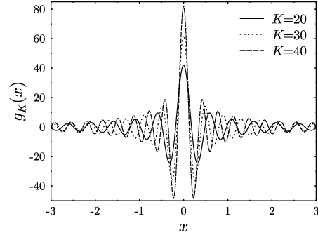
can be considered to be a regularized kernel function for the parity operator. In Fig. 6 we plot this function for increasing values of the cut–off parameter $K$ . It is seen that the singularity of the kernel function in the limit $K\rightarrow\infty$ is reflected by an oscillatory behaviour around $x=0$ with growing both the amplitude and the frequency. This amplifies the statistical uncertainty of the experimental homodyne data. In Fig. 7 we show determination of the parity operator for the three states discussed before, using increasing values of the cut–off parameter $K$ . Though we are in the region where the true photon number distribution is negligibly small, addition of subsequent matrix elements increases the statistical error in an approximately linear manner. This is easily understood, if we look again at the reconstructed photon number distributions: increasing $K$ by one means a contribution of the order of $\sqrt{2/N}$ added to the statistical uncertainty, and, moreover, these contributions tend to have the same sign due to correlations between the consecutive matrix elements. Thus, determination of the parity operator from homodyne statistics requires an application of a certain regularization procedure. It may be either the filtering used in tomographic back–projection algorithms, or the cut–off of the photon number distribution. The statistical uncertainty of the final outcome is eventually a result of an interplay between the number of experimental runs and the applied regularization scheme.

Finally, let us briefly comment on the compensation for the nonunit efficiency of the homodyne detector. First, one might think of applying a two–mode inverse Bernoulli transformation directly to the joint count statistics on the detectors. However, it is impossible in the homodyne scheme to resolve contributions from single absorbed photons due to high intensity of the detected fields. The inverse Bernoulli transformation has no continuous limit, as consecutive count probabilities are added with opposite signs. Nevertheless, the nonunit detection efficiency can be taken into account in the pattern functions [4]. In this case the statistical errors increase dramatically, and explode with $\nu\rightarrow\infty$ , which makes determination of the parity operator even more problematic. This is easily understood within the phase space picture: the distributions measured by an imperfect homodyne detector are smeared–out by a convolution with a Gaussian function [27, 28]. Evaluation of the parity operator, or equivalently, the Wigner function at the phase space origin requires application of a deconvolution procedure, which enormously amplifies the statistical error [29].

IV Conclusions

We have presented a complete statistical analysis of determining quantum observables in optical measurement schemes based on photodetection. We have derived an exact expression for the generating function characterizing statistical moments of the reconstructed observables, which, in particular, provides formulae for statistical errors and correlations between the determined quantities. These general results have been applied to the detection of phase–independent properties of a single light mode using two schemes: direct photon counting, and random phase homodyne detection. This study has revealed difficulties related to the completeness of the reconstructed information on the quantum state: in some cases the parity observable, which is a well–behaved bounded operator, effectively cannot be evaluated from the reconstructed data due to the exploding statistical error.

We have recalled that the parity operator is directly related to the value of the Wigner function at the phase space origin. Thus, our example can also be interpreted as a particular case of the transformation between two representations of the quantum state: in fact, we have considered evaluation of the Wigner function at a specific point $(0,0)$ from the relevant elements of the density matrix in the Fock basis. Therefore, our discussion exemplifies subtleties related to the transition between various quantum state representations, when we deal with data reconstructed in experiments. Though a certain representation can be determined with the statistical uncertainty which seems to be reasonably small, it effectively cannot be converted to another one due to accumulating statistical errors.

The presented study suggests that the notion of completeness in quantum state measurements should inherently take into account the statistical uncertainty. From a theoretical point of view, the quantum state can be characterized in many different ways which are equivalent as long as expectation values of quantum operators are known with perfect accuracy. In a real experiment, however, we always have to keep in mind the specific experimental scheme used to perform the measurement. This scheme defines statistical properties of the reconstructed quantities, and may effectively limit the available information on the quantum state. Determination of a family of observables does not automatically guarantee the feasibility of reconstructing the expectation value of an arbitrary well behaved operator. Reconstruction of any observable should be preceded by an analysis how significantly the final result is affected by statistical noise corrupting the raw experimental data.

Acknowledgements

The author is indebted to Professor K. Wódkiewicz for numerous discussions and valuable comments on the manuscript. This research was supported by the Polish KBN grant No. 2P03B 002 14 and by Stypendium Krajowe dla Młodych Naukowców Fundacji na rzecz Nauki Polskiej.

References

[1] D. T. Smithey, M. Beck, M. G. Raymer, and A. Faridani, Phys. Rev. Lett. 70, 1244 (1993).
[2] D. T. Smithey, M. Beck, J. Cooper, M. G. Raymer, and A. Faridani, Phys. Scr. T48, 35 (1993); M. G. Raymer, J. Cooper, H. J. Carmichael, M. Beck and D. T. Smithey, J. Opt. Soc. Am. B12, 1801 (1995).
[3] G. Breitenbach, T. Müller, S. F. Pereira, J.-Ph. Poizat, S. Schiller, and J. Mlynek, J. Opt. Soc. Am. B 12, 2304 (1995); S. Schiller, G. Breitenbach, S. F. Pereira, T. Müller, and J. Mlynek, Phys. Rev. Lett. 77, 2933 (1996); G. Breitenbach, S. Schiller, and J. Mlynek, Nature 387, 471 (1997).
[4] G. M. D’Ariano, C. Macchiavello, and M. G. A. Paris, Phys. Rev. A 50, 4298 (1994); G. M. D’Ariano, U. Leonhardt, and H. Paul, Phys. Rev. A 52, R1801 (1995); U. Leonhardt, H. Paul, and G. M. D’Ariano, Phys. Rev. A 52, 4899 (1995).
[5] U. Leonhardt, M. Munroe, T. Kiss, Th. Richter, and M. G. Raymer, Opt. Commun. 127, 144 (1996).
[6] G. M. D’Ariano, C. Macchiavello, and N. Sterpi, Quantum Semiclass. Opt. 9, 929 (1997).
[7] G. M. D’Ariano and M. G. A. Paris, Phys. Lett. A231, 325 (1997).
[8] U. Leonhardt and M. Munroe, Phys. Rev. A 54, 3682 (1996).
[9] P. J. Bardroff, E. Mayr, and W. P. Schleich, Phys. Rev. A 51, 4963 (1995).
[10] H. Paul, P. Törmä, T. Kiss, and I. Jex, Phys. Rev. Lett. 76, 2464 (1996).
[11] S. Wallentowitz and W. Vogel, Phys. Rev. A 53, 4528 (1996).
[12] K. Banaszek and K. Wódkiewicz, Phys. Rev. Lett. 76, 4344 (1996).
[13] A. Zucchetti, W. Vogel, M. Tasche, and D.-G. Welsch, Phys. Rev. A 54, 1678 (1996).
[14] K. Jacobs, P. L. Knight, and V. Vedral, J. Mod. Opt. 44, 2427 (1997).
[15] N. G. Walker and J. E. Caroll, Opt. Quant. Electron. 18, 355 (1986); J. W. Noh, A. Fougères, and L. Mandel, Phys. Rev. Lett. 67, 1426 (1991).
[16] V. Bužek, G. Adam, and G. Drobný, Phys. Rev. A 53, 3822 (1996).
[17] T. Opatrný, D.-G. Welsch, and W. Vogel, Phys. Rev. A 56, 1788 (1997); S. M. Tan, J. Mod. Opt. 44, 2233 (1997).
[18] Z. Hradil, Phys. Rev. A 55, R1561 (1997).
[19] K. Banaszek, Phys. Rev. A (in press).
[20] K. Banaszek and K. Wódkiewicz, J. Mod. Opt. 44, 2441 (1997).
[21] P. L. Kelley and W. H. Kleiner, Phys. Rev. 136, A316 (1964).
[22] T. Kiss, U. Herzog, and U. Leonhardt, Phys. Rev. A 52, 2433 (1995).
[23] M. Munroe, D. Boggavarapu, M. E. Anderson, and M. G. Raymer, Phys. Rev. A 52, R924 (1995).
[24] A. Royer, Phys. Rev. A 15, 449 (1977).
[25] H. Moya-Cessa and P. L. Knight, Phys. Rev. A 48, 2479 (1993)
[26] U. Leonhardt and I. Jex, Phys. Rev. A 49, R1555 (1994).
[27] W. Vogel and J. Grabow, Phys. Rev. A 47, 4277 (1993).
[28] U. Leonhardt and H. Paul, Phys. Rev. A 48, 4598 (1993).
[29] U. Leonhardt and H. Paul, J. Mod. Opt. 41, 1427 (1994).

Refer to caption — Figure 1: Reconstruction of the photon number distribution from photon counting for (a) a coherent state with $\langle\hat{n}\rangle=4$ , (b) a squeezed vacuum state with $\langle\hat{n}\rangle=1$ , and (c) a thermal state with $\langle\hat{n}\rangle=2$ , from $N=4000$ runs in each case. Monte Carlo simulations of a photon counting experiment, depicted with points, are compared with exact values (solid lines), with the statistical errors $[\text{Var}(\rho_{\nu})]^{1/2}$ marked as grey areas. The detection efficiency is $\eta=80\%$ .