Bures Metrics for Certain High-Dimensional Quantum Systems

Some five years ago, Hübner [1] (cf. [2]), in an article entitled, “Explicit computation of the Bures distance for density matrices,” derived a general formula for the Bures or statistical distance [3] ($d_{B}$) for $n$-dimensional density matrices ($\rho$). It took the form,

where $\mbox{d}\rho$ is the incremental change in $\rho$, and $\lambda_{i}$ is the $i$-th eigenvalue corresponding to the eigenvector $<i|$ of $\rho$.

Dittmann [4] has indicated how formula (1) can be reexpressed — using the Cayley-Hamilton identity — in terms of certain matrix invariants (thus, obviating any need for the eigenvalues and eigenvectors themselves). Slater [5] has applied Dittmann’s formula for the case $n=3$ to a set of four-parameter $3\times 3$ density matrices. (More recently still [6], we have relatedly examined the full eight-dimensional convex set of $3\times 3$, that is spin-1 density matrices.) In an infinite-dimensional (but three-parameter) setting, Twamley [7] has found the Bures metric for squeezed thermal states. Slater [8] utilized these results to find the corresponding volume element (which turns out to be simply the product of a function of the squeeze factor and a function of the inverse temperature, the phase being irrelevant in this regard). The volume elements of Bures metrics are of particular interest in that — if normalizable — they can be considered to form prior probability distributions (for purposes of Bayesian inference) over the associated quantum systems [9]. Twamley [7] has also suggested that a physical significance can be attributed to the scalar curvature of the Bures metric, in providing a parameterization (coordinate) independent measure of the accuracy of estimation of a state, given a reference state. (Scalar curvatures of Riemannian metrics on thermodynamic state spaces have been a subject of considerable analysis [10, 11].)

In this communication, we make direct use of the formula of Hübner (1) to obtain the restriction of the Bures metric for two different series of sets of $2^{n}\times 2^{n}$ density matrices of interest. In general, it requires $2^{2n}-1$ parameters to specify a $2^{n}\times 2^{n}$ density matrix. In light of the consequent severe computational demands entailed, we will limit our attention here to certain quite special density matrices, requiring but one or two parameters for their specification. We bring to the reader’s attention, however, Hübner’s remark: “The Bures metric is defined on the whole [emphasis his] space of density matrices” [2, p. 224].

We examine the associated normalized volume elements and the Gaussian curvatures for these restricted metrics. We note that in two dimensions — the framework of our first series of analyses — the Gaussian curvature is simply equal to the negative of one-half of the scalar curvature [12, p. 184]. In one dimension — the framework of our second series of analyses — there is no nontrivial notion of [intrinsic] curvature.

The starting point for our first series of analyses is the convex set of $2\times 2$ density matrices having real entries. Its members ($n=1$) are expressible as

where $(r,\theta)$ are polar coordinates ($0\leq r\leq 1$, $0\leq\theta<2\pi$), parameterizing the unit disk. An application of formula (1) to the density matrices (2) yields the Bures metric,

where

and

We observe that the elements of the metric (4) - (6) are independent of the angular parameter $\theta$. Normalizing the area (the form, of course, which “volume” takes in two dimensions) element ($\sqrt{\det{g}}=\sqrt{g_{rr}g_{\theta\theta}}$) over the unit disk, we obtain the prior probability distribution,

We have also applied Hübner’s formula (1) to the $n-$fold tensor product of the density matrix (2) with itself — corresponding to $n$ identical, independent two-level real quantum systems — for $n=2,\ldots,7$, and obtained, in all these six cases, results of the form,

and

(The eigenvalues and eigenvectors — to be used in (1) — of the $n$-fold products are directly derivable through basic rules from those of $\rho_{real}$ itself.) Since $g_{r\theta}$ has been found to equal zero, for $n=1,\ldots,7$, the polar coordinates ($r,\theta$) comprise an orthogonal curvilinear (Lamé) coordinate system in these instances, and presumably for all $n$. (The system is not isothermal or conformal [13, 14], however, in that $g_{rr}\neq g_{\theta\theta}$ — not even for a single value of $r\in[0,1]$.)

We have, following the lead of Twamley [7], computed the Gaussian curvature ($K$) — which equals one-half of the negative of the scalar curvature [12, p. 184] — of the Bures metrics reported above. For our orthogonal (polar) coordinate system, this takes the form [15, p. 105],

For $n=1,\ldots,7$, we have that $K={4\over n}$, that is, the $2^{n}\times 2^{n}$ density matrices form spaces of constant positive Gaussian curvature. (Braunstein and Milburn [17] have noted that: “there is an overall $\sqrt{N}$ improvement in the precision to which we may determine the parameter $X$ as we increase the number of identically prepared systems we can make measurements upon. This is familiar to us as the typical improvement upon increasing our sample size; here we see that it is a general limit to how well we can determine a parameter from quantum systems.”)

We have also conducted a more limited analysis of the $2\times 2$ density matrices with complex entries. These are parameterizable using spherical coordinates $(r,\theta,\phi)$ in the form,

The associated Bures metric,

for $n=1$, has elements (cf. [16, formula (15)]), being independent of the longitudinal coordinate $\phi$,

and

The volume element of this metric is normalizable to the prior probability distribution,

over the Bloch sphere [17] of two-level quantum systems, that is, the unit ball in three-space ($0\leq r\leq 1$, $0\leq\theta<\pi$, $0\leq\phi<2\pi$). The (Ricci) scalar curvature of this metric is equal to -24. We have been able to compute the Bures metric for the two-fold tensor products of $\rho_{complex}$ with itself, but the metric elements were given by highly involved algebraic expressions, which proved difficult to simplify. However, by setting $r,\theta,\phi$ to specific values a number of times, we obtained results, in all these cases, fully consistent with the proposition that these elements are, in fact, simply twice those given by ((14)-(16). (The scalar curvature would, then, be equal to -12.) This would adhere to the pattern noted above (for $n=2,\ldots,7$) with the $2\times 2$ real density matrices. Presumably, there exists a demonstrable theorem confirming that this rule holds for all $n$, for both the real and complex $2\times 2$ density matrices and, possibly other types of density matrices, as well. (The space of $n\times n$ density matrices, for $n>2$, “is not a space of constant curvature and not even a locally symmetric space, in contrast to what the case of two-dimensional density matrices might suggest” [4].)

In our other series of analyses, we also apply the formula (1) of Hübner to a series of $2^{n}\times 2^{n}$ density matrices ($n=2,\ldots,7$). Rather than the pair of polar coordinates ($r,\theta$), as in the first instance, these density matrices are parameterized in terms of a single variable ($u$ or alternatively, $\beta$ — as elaborated below). The intial (universal quantum coding) motivation for studying them was presented in an extended paper of Krattenthaler and Slater [18]. These $2^{n}\times 2^{n}$ density matrices were obtained by averaging (over the Bloch sphere of two-level quantum systems) the $n$-fold tensor products with themselves — corresponding to $n$ independent, identical systems — of the $2\times 2$ complex density matrices (12). (An analogous [unpublished] study has also been conducted, using the $2\times 2$ real density matrices, but the proofs of certain propositions have turned out — somewhat surprisingly — to be more problematical, involving an intricate triple summation, in that [lower-dimensional] context.) The averaging was performed with respect to a one-parameter ($u$) family of probability distributions,

In [19] it was argued that this family (19) could be given a thermodynamic interpretation by using the changes-of-variable, $u=1-\beta$ and $r=\sqrt{1-e^{-E}}$. One, then, arrives at a Gibbs distribution of the form,

where the energy $E$ is taken to be the negative of $\log(1-r^{2})$, the density-of-states or structure function, $\Omega(E)$, to be $\sqrt{1-e^{-E}}$, and the partition function to be

The natural interpretation of the parameter $\beta$ appears to be that of an effective polarization temperature [19, 20] (cf. [21, 22]).

Explicit formulas were reported in [18] for the eigenvalues and eigenvectors of the $2^{n}\times 2^{n}$ matrices $(\zeta_{n}(\beta))$ averaged with respect to (19). It was found that there are only $1+\lfloor n/2\rfloor$ distinct eigenvalues. The eigenvectors constructed in [18] formed bases of the $1+\lfloor n/2\rfloor$ subspaces, but were not orthogonalized within the subspaces (cf. [23, pp. 426-427]). The eigenvalues can be expressed as

with respective multiplicities,

The subspace spanned by the $m_{n,q}$ eigenvectors for the eigenvalue $\lambda_{n,q}$ corresponds to those explicit spin states [23, sec, 7.5.j] [24] with $q$ spins either “up” or “down” (and the other $n-q$ spins, of course, the reverse). The $2^{n}$-dimensional Hilbert space can be decomposed into the direct sum of carrier spaces of irreducible representations of $SU(2)\times S_{n}$. The multiplicities (23) are the dimensions of the corresponding irreps. The $q$-th subspace consists of the union of $m_{n,q}/(n-2q+1)$ copies of irreducible representations of $SU(2)$, each of dimension $(n-2q+1)$ or, alternatively, of ($n-2q+1$) copies of irreps of $S_{n}$, each of dimension $m_{n,q}/(n-2q+1)$.

The Bures metrics for the six cases ($n=2,\dots,7$) analyzed, take the simple form, $g_{\beta\beta}\mbox{d}\beta^{2}$. We have found that $g_{\beta\beta}$ equals

for $n=6$, the ratio of

to

and for $n=7$, the ratio of

to

For this series of computations, we used MATHEMATICA to obtain fully orthonormal sets of eigenvectors. In doing so, for $n>4$, computational considerations required us to resort to a somewhat indirect approach, not simply making use of the Eigensystem command, but rather the NullSpace command, coupled with our knowledge of the actual eigenvalues. (In all cases, however, it was necessary to, additionally, employ the GramSchmidt command on the vectors yielded by the Eigensystem or NullSpace command.) Since our singly-parameterized matrices for a given $n$ all commute, we could have relied upon Hübner’s formula [1, p. 242],

“which is simply the Hilbert-Schmidt metric, not on the space of density matrices itself, but on the ‘space of roots of density matrices’ rather” [1].

The numerators of the results ((24), (25)) for $n=2,3$ are simply constants. For $n>3$, the roots of the numerators also have negative real parts lying between -1 and $-n$. It is clear from immediate inspection that all the roots of the denominators for $n=2,\ldots,7$, except for 0, are no greater than -1. There are, of course, singularities of $g_{\beta\beta}$ at 0 for all these $n$, and at the other (strictly negative) roots of the denominator.

In Fig. 1, we plot $g_{\beta\beta}$ for $n=2,\ldots,7$. (There is no nontrivial concept of intrinsic curvature for one-dimensional metrics. In this regard, however, it is of interest to note that in his study of squeezed thermal states, Twamley [7] finds that the “curvature is independent of the ’unitary’ parameters $r$ and $\theta$ and only depends on the ‘non-unitary’ parameter $\beta$.) The curve for $n=7$ dominates that for $n=6$, which, in turn, dominates that for $n=5,\ldots$ All the curves are monotonically decreasing with $\beta$.

The elements of length ($\sqrt{g_{\beta\beta}}$) can be normalized over the range $\beta\in[0,\infty]$ by dividing $\sqrt{g_{\beta\beta}}$ by $\pi/6\approx$ .523599 ($n$=2), $\pi/4\approx.785398$ ($n=3$), .987405 ($n=4$), 1.1533 ($n=5$), 1.29428 ($n=6$) and 1.42688 ($n=7$).

From [18, formula (2.12)], that is, formula (22) above, we know the eigenvalues of the averaged matrices for arbitrary $n$. Since any two averaged matrices $(\zeta_{n}(\beta_{1}),\zeta_{n}(\beta_{2}))$ for distinct values of $\beta$ are known from [18] to share the same set of eigenvectors — so, $\zeta_{n}(\beta_{1})$ and $\zeta_{n}(\beta_{2})$ necessarily commute — the eigenvalues themselves are all that is required to compute the (in general, nonlocal) Bures distance between the density matrices. (I thank C. Krattenthaler for pointing this out.) This can be deduced from the general formula for the Bures distance [1],

Employing (29) for the case $n=2$, by setting $\rho_{1}=\zeta_{2}(\beta_{1}),\rho_{2}=\zeta_{2}(\beta_{2})$, we obtain

Also, for $n=3$,

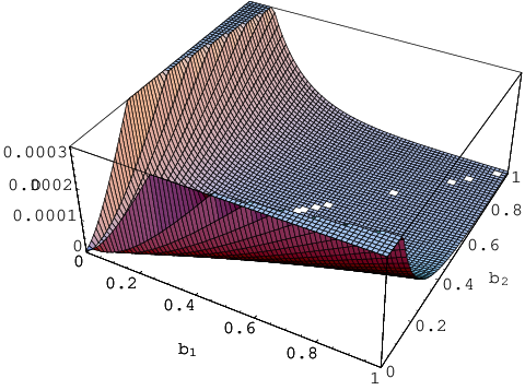
In Fig. 2, making a more intensive use of the eigenvalue formula (22), we plot the Bures distance ($d_{B}$) between $\zeta_{100}(\beta_{1})$ and $\zeta_{100}(\beta_{2})$.

(Of course, the value of $d_{B}$ along the line $\beta_{1}=\beta_{2}$ is zero.) The function shown in this figure is computed as

Given the Bures distance, we would, then, be able to obtain, the Bures metric, through the use of the formula [1, p. 241],

Employing such an approach to finding $g_{\beta\beta}$, would avoid having to compute the eigenvectors of the matrices $\zeta_{n}(\beta)$. (We, in fact, found the computation of the eigenvectors of the $256\times 256$ density matrices, $\zeta_{8}(\beta)$, to be beyond our resources.)

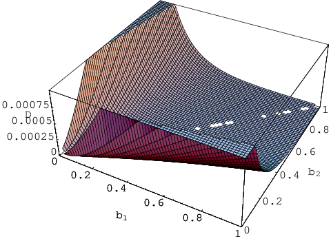
Let us, making use of (24), compare the integrated element of length

with the Bures distance itself (30) between $\zeta_{2}(\beta_{1})$ and $\zeta_{2}(\beta_{2})$. In Fig. 3, we plot the absolute value of this function (34) minus the Bures distance — given by (30).

In Fig. 4, we display the analogous result for the case $n=3$, making use of (31) and the relation,

For $n>3$, it appeared it would be necessary to employ numerical integration to evaluate $\int_{\beta_{1}}^{\beta_{2}}\sqrt{g_{\beta\beta}}\mbox{d}\beta$ to generate similar figures.

It would be of interest to study the question of whether or not the Bures distance between $\zeta_{n}(\beta_{1})$ and $\zeta_{n}(\beta_{2})$ can be achieved for some particular (geodesic) path through the unrestricted $(2^{2n}-1)$-dimensional parameter space of the $2^{n}\times 2^{n}$ density matrices (cf. [17]).