Exact two-loop vacuum polarization correction
to the Lamb shift in hydrogen-like ions
Günter Plunien, Thomas Beier and Gerhard Soff
Institut für Theoretische Physik, Technische Universität Dresden,
Mommsenstr. 13, D-01062 Dresden, Federal Republic of Germany
Hans Persson
Department of Physics, Chalmers University of Technology and
the University of Gothenburg, S-412 96 Göteborg, Sweden
PACS-numbers: 31.10.+z, 31.30.-i, 31.30.Jv
Abstract
We present a calculation scheme for the two-loop vacuum polarization correction of order to the Lamb shift of hydrogen-like high- atoms. The interaction with the external Coulomb field is taken into account to all orders in . By means of a modified potential approach the problem is reduced to the evaluation of effective one-loop vacuum polarization potentials. An expression for the energy shift is deduced within the framework of partial wave decomposition performing appropriate subtractions. Exact results for the two-loop vacuum polarization contribution to the Lamb shift of K- and L-shell electron states in hydrogen-like Lead and Uranium are presented.
I Introduction
Recent experimental progress in the spectroscopy of highly charged heavy ions [1, 2, 3, 4] demands theoretical predictions for the Lamb shift, which should include the complete set of QED radiative corrections of order but accounting for all orders in the interaction with the strong external Coulomb field. For low- elements, a potential expansion with respect to powers in is legitimate and all -corrections have recently been calculated up to the order of [5, 6]. However, for systems under consideration in recent Lamb-shift measurements such as Gold or Uranium, a value for the effective coupling already indicates that -expansion in the regime of large becomes inadequate. Instead, exact electron propagators and wave functions in the external Coulomb field of extended nuclei have to be used in calculations of all second-order diagrams (Fig. 1). Meanwhile, calculational approaches are available for most of these QED effects (see the work of Persson et al. [7] and cited references). However, the calculations are not yet complete: 1. Exact numerical evaluations of the complete set of two-photon self-energy contributions remains as a major challenge, although recent progress has been made in deriving renormalized expressions for the resulting energy shifts [12]. The lack of numerical results for these contributions represents a major uncertainy in theoretical predictions for the Lamb shift aiming for a relative precision of for the total electron binding energy. 2. Exact evaluation schemes, which also treat the loops involved to all orders in , have been developed [14] only for the combined self energy - vacuum polarization corrections SEVPabc and the two-loop ladder vacuum polarization diagram VPVPa (see Fig. 1). Values for the VPVPa correction for large -numbers have been tabulated recently [8]. The self energy-vacuum polarization S(VP)E (Fig. 1) is calculated by employing the Uehling-approximation for the loop [7]. Calculation of the higher-order contribution to this diagram are presently in progress. 3. Until now, the two-loop diagram VPVPb as well as the self energy corrected one-loop vacuum polarization contribution VPVPc (Fig. 1) where calculated only to lowest order in utilizing the Källén-Sabry polarization function [11, 9, 10].
Aiming towards the completion of the exact evaluation of all QED-radiative corrections of order , we shall present a calculation scheme which allows the higher-order -contribution of the two-loop vacuum polarization correction VPVPb to be determined. Recognizing that the diagram we wish to calculate is part of the complete ”dressed” one-loop vacuum polarization allows us to reduce the problem to the evaluation of effective one-loop corrections where the renormalization procedure is known [13, 15].
Section II contains a general discussion of ”dressed” electron propagators in arbitrary, classical external fields and of the induced vacuum polarization. In section III we specify the formulae to the situation in hydrogen-like ions. The subtraction scheme for deducing the two-loop correction from various effective one-loop contributions will be introduced. Section IV briefly reviews the renormalization procedure. An expression for the renormalized energy shift due to the higher-order (in ) part is derived. This consists of two terms which require a different numerical treatment. In order to compare the effect due to higher orders in we also present results for the two-loop correction in Uehling approximation, which will be derived in section V. In section VI we will calculate the effect of the higher-order contribution to the S-Lamb shift in hydrogen-like Lead and Uranium.
Throughout this paper, units will be used where and .
II Dressed electron propagators and one-loop vacuum polarization
We start with a brief discussion of the concept of ”dressed” electron propagators and of the corresponding ”dressed” one-loop vacuum polarization (VP). Some general formulae will be derived, which will be employed in the next section.
We shall adopt the term ”dressed” electron (positron) line for an electron (positron) moving in an arbitrary, external electromagnetic field . The wave function that accounts for the interaction with this external field is a solution of the Dirac equation:
| (1) |
Choosing free electron lines as a reference, we shall refer to the state as ”-dressed” electron line. Similarly, an electron interacting with the external Coulomb-potential generated by the (bare) nuclear charge density distribution may be called a ”Coulomb-dressed” electron. In general situations it is appropriate to divide the total external field into two parts and , i.e.:
| (2) |
where e.g. the second term may be considered a perturbation. Accordingly, considering electron states in the external field as unperturbed states, we may then call these states ”-dressed”. The propagators and describing electrons in the external field respectively are defined by
| (3) |
Note that they also satisfy the equations
| (4) |
where the (adjoint) Dirac-operators are acting to the left. In analogy to the Dyson equation defining dressed propagators in terms of improper self-energy insertions etc. we postulate an equation of the form
| (5) |
with a kernel . With the aid of equations (II) and (II) we can solve for the kernel:
| (6) |
Insertion of Eq. (6) into (5) leads to an equation for the ”-dressed” propagator (taking as the reference) which can be solved iteratively. The exact propagator appears as the sum of the unperturbed external field propagator , a part describing a single-scattering with the additional external field and a higher-order part which accounts for multiple-scattering contributions. Given a representation for a formal expression for the corresponding one-loop vacuum-polarization current induced by the total external field can be derived. For later purposes we will already specialize to the case of static external fields. Since the propagators are homogeneous in time, one obtains:
| (7) | |||||
Putting aside questions about renormalization for a moment, this formally exact equation implies that the one-loop vacuum polarization induced by the total field is given as a sum of three terms: a part induced by the external field , a single-interaction contribution and a third part taking into account multiple interactions with the additional external field .
The representation of the propagator and of the induced vacuum polarization derived above are not unique. The reason for this is provided by the fact that the decomposition of the total external field (2) is completely arbitrary. In particular, we could have chosen the free-field configuration as unperturbed reference. Consequently, the external field propagator in the defining equation (5) has to be replaced by the free Feynman propagator leading to a similar kernel (6) which will contain the total external field . In this case Eq. (7) takes the form
The free closed-loop contribution vanishes in accordance with the Furry-theorem. The induced vacuum polarization itself gives rise to a modification of the total external field:
| (9) |
The free photon propagator is given by (in Feynman gauge)
| (10) | |||||
The last line of the expression above specifies the partial wave decomposition of the photon propagator. A spherically symmetric, static external potential induces only a static vacuum polarization charge density which will also be spherically symmetric. It gives rise to an effective one-loop VP-potential:
| (11) |
III Subtraction scheme
The general considerations of the previous section may have already anticipated how we are going to deduce the two-loop vacuum polarization correction. The basic idea is to derive this contribution from an effective one-loop vacuum polarization , which is dressed with the renormalized first-order vacuum polarization potential induced by the external Coulomb field of the nucleus. At first we need to specialize Eq. (7) to (11) to the situation of bound-state QED. In the presence of a static, spherically symmetric nuclear charge density, we specify the total external field (2) as the sum of the (bare) external Coulomb potential and the renormalized, first-order vacuum polarization potential :
| (12) |
The one-loop potential is obtained from
| (13) |
after renormalization. denotes the electron propagator in the external Coulomb field. In view of Eqs. (7) and (11) the VP-dressed one-loop vacuum polarization potential formally reads
| (14) | |||||
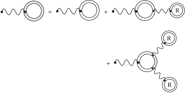
A graphical representation of the VP-dressed one-loop potential is depicted in Fig. 2. The two-loop vacuum polarization correction we are interested in appears as the second term of the decomposition (14) together with the ordinary one-loop vacuum polarization (first term). The third term accounts for all multiple interaction terms and is at least of order , since the additional potential contributes with a leading order (Uehling-term). Thus, it is legitimate to neglect this higher-order part. Consequently, we identify as the renormalized two-loop potential
| (15) | |||||
after appropriate renormalizations have been applied to the right-hand side of the above equation. Note, however, that the formal expression for the effective one-loop vacuum polarization density (first term in the curly brackets) already contains the renormalized one-loop potential , assuming that the renormalization of the exterior VP-loops can be performed separately. This issue will be adressed in the next section. We are now in the position to write down the energy shift of a bound electron state due to the exact two-loop correction:
| (16) |
In order to deduce exclusively the contribution arising from higher orders in , one has to subtract the corresponding two-loop contribution evaluated in the Uehling-approximation.
IV Renormalization
Taking the above into consideration, the problem of renormalization of the exact two-loop potential
| (17) | |||||
reduces to the problem of renormalization of the one-loop vacuum polarization. This is sugguested by Eqs. (14) and (15). It relies on the fact, that the external VP-loop is properly taken into account in terms of a VP-dressed effective one-loop, where the external VP-loop may be replaced by the renormalized first-order potential . This is supported by the notion that the electron (positron) experiences the effective nuclear charge modified by the induced vacuum polarization cloud. Procedures for renormalization of one-loop potentials involved in Eq. (15) are well known from the evaluation of the energy shift due to the first-order vacuum polarization in external Coulomb fields. We adopt the partial wave decomposition approach together with the subtraction scheme developed in [13, 15] and apply it to Eq. (15). In order to perform similar steps as in the case of the ordinary Coulomb-dressed VP-loop, we employ the equivalent representation according to Eq. (II)
| (18) | |||||
where denotes the total external potential Eq. (12). Fig. 3 shows the diagrammatic representation of Eq. (18). Further evaluation requires a partial wave decomposion of all the propagators
| (19) |
together with Eq. (10) for the photon propagator. According to the renormalization prescription developed in [15] the renormalized one-loop potential is obtained as the sum of the finite ”Wichmann-Kroll”-type contribution and of the renormalized ”Uehling”-type potential . We are lead to the following expressions:
| (20) |
together with the radial kernel
| (21) |
denotes the sum of the (bare) nuclear charge density and of the renormalized first-order vacuum polarization charge density induced by the Coulomb field of the nucleus. Eqs. (IV) and (IV) are analogous to expressions one has to deal with when deriving the renormalized, exact one-loop potential (13). Performing now the subtraction as implied by Eq. (15), we identify the renormalized two-loop vacuum polarization potential:
| (22) | |||||
| (23) | |||||
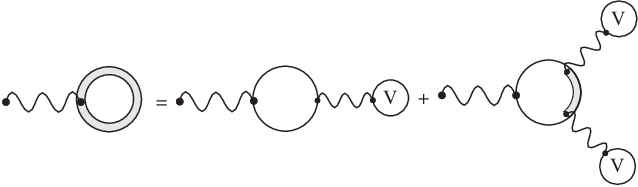
The term denotes the finite (renormalized) Uehling-type potential generated by the Uehling part of the renormalized first-order vacuum polarization charge density. The term summarizes the finite part of the Wichmann-Kroll-type potential. Since the sum over partial waves terminates at some finite each contribution in square brackets becomes well defined. The procedure described in Eqs. (22) to (IV) for deducing the renormalized exact two-loop vacuum polarization potential is depicted in Fig. 4.
For numerical evaluations, however, the representation (IV) of the potential is ruther cumbersome since it involves terms given as multiple summations over the free Dirac spectrum. A representation which is more convenient for numerical calculations can be introduced as follows: At first, we combine the one-potential terms in Eq. (IV) to a one-potential term involving the renormalized one-loop vacuum potential only. Secondly, the resulting one-potential term is replaced by the completely VP-dressed (free) one-loop potential assuming that the effects due to multiple-interaction contributions, which are at least of order , are neglegible. Thus we obtain the alternative representation:
where the states are solutions of the Dirac equation with the external potential and corresponding energy eigenvalues .
Having derived the renormalized potential , the corresponding energy shift of a bound electron state in the external Coulomb field can be evaluated according to (16).
V Two-loop contribution in Uehling approximation
Being interested primarily in the contribution to the energy shift due to higher orders in , we should subtract the Uehling-in-Uehling contribution, where the exact vacuum polarization loops are replaced by free fermion loops. Taking a uniform sphere model for the nuclear charge distribution, i.e. , the latter reads:
| (26) | |||||
The expression for may be cast into the more familiar form:
| (27) | |||||
This vacuum polarization charge density is plotted in Fig. 6. It is easily verified that the induced Uehling density (27) possesses a logarithmic singularity at the nuclear radius, which originates from the first term in the curly brackets. Integrating the Uehling charge density over the interior of the nucleus we obtain the finite induced vacuum charge
| (28) | |||||
which is exactly cancelled by the total induced charge in the exterior region .
The corresponding energy correction to the binding energy – we refer to it as Uehling-in-Uehling correction – which is part of the Källén-Sabry correction [10] reads:
| (29) |
This will be calculated separately.
VI Evaluation
We now turn to the evaluation of the higher-oder ()-contribution of the two-loop vacuum polarization to the Lamb shift of strongly bound electrons
| (30) |
where the Uehling-in-Uehling part is subtracted. Thus the effect of all higher orders in in the interaction with the external Coulomb potential contributing to the exact two-loop correction proceeds in two separate steps. Accordingly, we only need to calculate the renormalized Uehling-potential generated exclusively by the induced Wichmann-Kroll charge density
| (31) |
and the renormalized Wichmann-Kroll-type Potential according to the subtraction scheme (IV).
As a first step towards the evaluation of the energy correction (30) we consider the contribution
| (32) |
This correction to the Lamb shift of the bound state is related to the change of the Uehling potential Eq. (31) arising from the Wichmann-Kroll part of the induced vacuum polarization. At first we wish to derive an estimate for this correction to the Lamb shift of the ground state in hydrogen-like Lead and Uranium.
The Wichmann-Kroll charge density is calculated based on the partial wave decomposition of the Coulomb propagator and of the free propagator as developed in Ref. [13]. It is obtained from
| (33) | |||||
where the summation over is terminated at some maximum value . The quantities and denote the partial wave decompositions of the free and the bound propagators. Apart from the long-range tail where the Wichmann-Kroll vacuum polarization charge density is positive, a strongly pronounced maximum of negative charge density occurs in the vincinity of the nuclear surface (see Ref. [13]). Integrating over this -range one obtains a total induced negative charge
| (34) |
Since the Wichmann-kroll density is strongly localized near the nuclear surface it acts almost like an additional negatively charged spherical shell surrounding the nucleus. A strongly bound electron experiences the reduced nuclear charge. This suggests replacing the corresponding potential by the Uehling potential generated by a spherical shell carrying the negative charge as an approximation. In this case the integral Eq. (31) can be evaluated imediately. If we further employ a spherical shell model for the nuclear charge distribution, a simple scaling-law is derived. This relates the energy shift Eq. (32) with the first-order Uehling correction according to:
| (35) |
The validity of this scaling-law is supported by the fact that the numerical results for the Uehling correction do not depend significantly upon details of the extended nuclear charge distribution. With the scaling-law at hand we have an additional tool for testing the numerical results for the Wichmann-Kroll-in-Uehling contribution Eq. (32) for strongly bound electrons.
VII Results and discussion
The scaling-law Eq. (35) derived above for the ”Wichmann-Kroll in Uehling” part may only be useful as test for its complete numerical calculation. In order to employ the scaling-law the first-order Uehling correction and the Wichmann-Kroll charge density need to be determined. This can be achieved by means of very accurate numerical procedures developed earlier (see e.g. [13, 15, 8] and references therein). For a discussion of technical details encountered with the evaluation of we refer to [8]. The total induced negative charge number is obtained by integrating the Wichmann-Kroll density from the origin up to where changes its sign. Table 1 gives numerical results for the first-order Uehling correction, the induced negative charge number and for the corresponding energy shifts according to the scaling-law for the S-ground state of hydrogen-like Lead and Uranium respectively. The energy correction is repulsive, since the induced charge is negative.
Let us compare the effect of the higher-order contribution to the two-loop correction defined by Eq. (30) with the one obtained in Uehling approximation . The latter is tabulated in the first column of Table 2 for K- and L- shell electrons in hydrogen-like Lead and Uranium. This Uehling-in-Uehling contribution is attractive and amounts to less than % of the total Källén-Sabry correction to the Lamb shift as tabulated in [10]. The results for the exact two-loop correction are tabulated in the second column of Table 2.
In comparison with the exact numerical results for the Wichmann-Kroll-in-Uehling contribution as presented in the third column of Table 2 the scaling-law indeed gives the right order of magnitude but leads to a systematic overestimation due to the neglection of the long-range tail of . The numerical results for the Wichmann-Kroll-type contribution , which have been obtained according to the representation (IV), are presented in the last column of Table 2. As for the Uehling-in-Uehling correction this contribution carries the same overall sign, i.e. it also acts attractive. It comprises about % of the two-loop diagram evaluated in Uehling approximation. This result also indicates that higher-order () contributions to the one-loop polarization insertion of the photon propagator may be not small compared with the Uehling approximation. Accordingly, it may be not surprising at all, if the higher-order contribution to the S(VP)E - correction (see Fig. 1) may turn out to be important as well.
Even in the case of Uranium the order of magnitude for the total higher-order part (see Table 2) is about eV for the 1S-state, which indicates that the effect of the higher-order contributions to the two-loop vacuum polarization alone are far too small to be detected via Lamb-shift measurements with current accuracies. Furthermore, this correction is about one order of magnitude below the natural limitations for tests of QED set by nuclear polarization effects [16]. It might also be instructive to compare this effect with the uncertainties of the S-energy level caused by the uncertainties in the determination of the nuclear radii. The rms-radius for Uranium is given by fm [17] and leads to an uncertainty of about eV. Although a complete numerical evaluation of the exact Källén-Sabry diagrams, i.e., the higher-order contributions of the self-energy-corrected one-loop diagram VPVPc remain to be performed, the goals of this paper have been achieved: 1. We have presented a calculational scheme for evaluating the two-loop vacuum polarization corrections to all orders in the interaction with the external Coulomb potential. The problem is reduced to the evaluation of an effective one-loop correction. Thus, the partial wave decomposition can be employed in a similar way as it has been used successfully in calculations of the ordinary first-order vacuum polarization correction. 2. Numerical results for exact two-loop vacuum polarization correction to the Lamb shift of K- and L-shell electrons in hydrogen-like Lead and Uranium have been obtained. It turns out to be below the natural limits set by nuclear polarization effects and by the uncertainties of nuclear parameters. 3. Although the effect of the higher-order contributions to the two-loop diagram turn out to be small a further uncertainty in Lamb-shift calculations has been eliminated. Aiming for a relative precision of of theoretical predictions of the binding energy we conjecture that the still unknown exact two-photon self energy corrections remain the major source of uncertainties.
Acknowledgements.
The authors are grateful to Sten Salomonson and Per Sunnergren for interesting discussions. Financial support has been provided by the BMBF, the DFG, the DAAD, the SI, and the GSI (Darmstadt).References
- [1] J. Schweppe, A. Belkacem, L. Blumenfeld, N. Claytor, B. Feinberg, H. Gould, V. E. Costram, L. Levy, S. Misawa, J. R. Mowat, and M. H. Prior, Phys. Rev. Lett. 66, 1434 (1991).
- [2] H. F. Beyer, D. Liesen, F. Bosch, K. D. Finlayson, M. Jung, O. Kleppner, R. Moshammer, K. Beckert, H. Eickhoff, B. Franzke, F. Nolden, P. Spädtker, M. Steck, G. Menzel, R. D. Deslattes, Phys. Lett. A184, 435 (1994).
- [3] Th. Stöhlker, P. H. Mokler, K. Beckert, F. Bosch, H. Eickhoff, B. Franzke, M. Jung, T. Kandler, O. Klepper, C. Kozhuharov, R. Moshammer, F. Nolden, H. Reich, P. Rymuza, P. Spädtke, and M. Steck, Phys. Rev. Lett. 71, 2184 (1993).
- [4]
H. F. Beyer, IEEE Trans. Instrum. Meas. 44, 510 (1995);
H. F. Beyer, G. Menzel, D. Liesen, A. Gallus, F. Bosch, R. Deslattes, P. Indelicato, Th. Stöhlker, O. Klepper, R. Moshammer, F. Nolden, H. Eickhoff, B. Franzke, and M. Steck, Z. Phys. D 35, 169 (1995). - [5]
M. I. Eides and H. Grotch, D. A. Owen,
Phys. Lett. B294, 115 (1992);
M. I. Eides and H. Grotch, Phys. Lett. B301, 127 (1993);
M. I. Eides and H. Grotch, Phys. Lett. B308, 389 (1993);
M. I. Eides, S. G. Karshenboim, and V. A. Shelyuto, Phys. Lett. B 312, 389 (1993);
M. I. Eides, H. Grotch, and P. Pebler, Phys. Rev. A50, 144 (1994).
- [6]
K. Pachucki, Phys. Rev. A48, 2609 (1993);
K. Pachucki, Phys. Rev. Lett. 72, 3154 (1994). - [7] H. Persson, I. Lindgren, L. Labzowsky, T. Beier, G. Plunien, and G. Soff, Phys. Rev. A 54, 2805 (1996).
- [8] T. Beier, M. Greiner, G. Plunien, and G. Soff, accepted for publication in J. Phys. B, (1997).
- [9] T. Beier and G. Soff, Z. Phys. D8, 129 (1988).
- [10] S. M. Schneider, W. Greiner, and G. Soff, J. Phys. B26, L529 (1993).
- [11] G. Källén and A. Sabry, Mat. Fys. Medd. Dan. Vid. Selsk. 29, 17 (1955)
- [12]
L. Labzowsky and A. O. Mitrushenkov,
Phys. Lett. A198, 333 (1995);
L. Labzowsky and A. O. Mitrushenkov, Phys. Rev. A53, 3029 (1996). - [13] G. Soff and P. J. Mohr, Phys. Rev. A 38 (1988) 5066.
- [14]
H. Persson, I. Lindgren, and S. Salomonson,
Phys. Scr. T46, 125 (1993);
I. Lindgren, H. Persson, S. Salomonson, and A. Ynnermann, Phys. Rev. A47, 4555 (1993). - [15] H. Persson, I. Lindgren, S. Salomonson, and P. Sunnergren, Phys. Rev. A48, 2772 (1993).
- [16]
G. Plunien, B. Müller, and W. Greiner, Phys. Rev. A43, 5853 (1991);
A. V. Nefiodov, L. N. Labzowsky, G. Plunien, and G. Soff, Phys. Lett. A188, 371 (1996);
A. V. Nefiodov, L. N. Labzowsky, G. Plunien, T. Beier, and G. Soff, J. Phys. B29, 3841 (1996). - [17] V. Zacek, H. Bohn, H. Brum, F. von Feilitzsch, G. Giorginis, P. Kienle, S. Schuhbeck, Z. Phys. A318, 7 (1984).
| system | |||
|---|---|---|---|
| U | |||
| Pb |
| system | state | ||||
|---|---|---|---|---|---|
| U | |||||
| Pb | |||||