A Generalization of Deutsch’s Example

A quantum computer is a quantum system whose time evolution can be thought of as a computation, much in the same way as we think of the time evolution of a pocket calculator to be a computation.

For our pourposes it will suffice to model the quantum system as a “black box” and focus our attention on two discrete observables out of a complete set, which we shall call the input and output register. Following the standard notation [1], we shall indicate the computation of a function $f:A\to B$ as

the first ket describing the state of the input register and the second the state of the output register. Kets are labelled according to the elements of $A$ and $B$ they represent.

One of the most powerful features of quantum computation is quantum parallelism. The superposition principle of quantum mechanics allows us to prepare the computer in a coherent superposition of a set $I\subseteq A$ of input states. After a single run, all of the corresponding outputs $f(x)$ appear in the final state, according to the time evolution

Unfortunately, this is no “pay one, take N”. In fact, the result is an entangled state of the input and output registers and there is no single measurement allowing us to extract from it all the computed values of $f(x)$ [2]. However, it may well be possible to distil from this final state some global property of the function, thus exploiting quantum parallelism. One of the most famous examples was presented by D. Deutsch, who showed that a single quantum computation may suffice to state whether a two–valued function of a two–valued variable is constant or not [2, 3]. D. Deutsch and R. Jozsa later generalized this result [4] showing that the problem of classifying a given function

as “not constant” or “not balanced” can be solved in polynomial time by means of a quantum computer (the time required by a classical solution is exponential). Also D. R. Simon showed that the problem of determining if a function is invariant under a so–called XOR mask, while it is classically intractable, admits an efficient quantum solution [5].

All of the algorithms cited above (apart from the last, for which Simon also considered a fully probabilistic generalization) are characterized by a variable running time and zero error probability. They consist of a non–classical computation like (1) followed by a measurement of the final state of the computer, as a result of which either the correct answer is obtained or the relevant information is destroyed and an explicitly inconclusive result is returned. In the latter case one has to go through the whole procedure again, so that only an average running time for the algorithm can be estimated.

Global properties of functions that can be determined by such an algorithm are said to be Computable by Quantum Parallelism (QPC).This definition was put forward by Jozsa [2] who also demonstrated that, at least in the case of two–valued functions, the QPC properties that can be determined by means of a single computation are an exponentially small fraction of all the possible global properties.

In this paper we tackle the general problem of stating whether a function

is constant or not.

We show that for $N>2$ or $M>2$ this property is not QPC, meaning that any measurement following a computation like (1) has a finite probability of yielding a wrong result. We therefore investigate the power of quantum parallelism in a fully probabilistic setting. Assuming that the (classical) computation of $f$ on $k$ randomly sampled points yields a constant value, we calculate the posterior probability that $f$ is actually constant. We then compute the analogous probability for a quantum algorithm requiring the same number of computations of $f$. Comparison of the two results shows that our quantum strategy allows making a better guess at the solution, its indications being more likely to be correct.

We shall now briefly recall the classical example put forward by D. Deutsch [3], before confronting the problem of its generalization. Suppose we are given a function $f:\{0,1\}\to\{0,1\}$ and we are interested to know whether $f$ is constant or not. Of course there are only four such functions (i.e. four instances of the problem), namely

If all we can use is a classical computer, there is only one way to do the job: we must compute both $f(0)$ and $f(1)$ and compare them to check if they are equal. On the contrary, since in this simple case the property “$f$ is constant” is QPC, a quantum computer gives us a fair chance of finding the solution at the cost of the single computation

After the computation, the calculator halts with its input and output registers in one of four possible states, corresponding to the four possible functions:

Since the above states are linearly dependent, they cannot be distinguished with certainty. This means that no measurement can establish which function was actually computed, or, which is the same, it’s impossible to extract from the final state both the values of $f(0)$ and $f(1)$. However, we need only discriminate $|f_{1}\rangle$ and $|f_{2}\rangle$, the final states yielded by the constant functions, from $|f_{3}\rangle$ and $|f_{4}\rangle$. This can actually be done by measuring on the final state of the two registers an observable with the following non–degenerate eigenstates:

These four states can be thought of as “flags” indicating the result of the computation and have been named according to their meaning. This becomes clearer as soon as we rewrite the final states (3) on the basis of the above eigenvectors:

It is now evident that

1. 1.

   projection along the eigenvector $|\mathrm{SAME\rangle}$ can only take place if the state of the computer is either $|f_{1}\rangle$ or $|f_{2}\rangle$, i.e. when $f$ is constant;

2. 2.

   likewise, projection along the eigenvector $|\mathrm{DIFFERENT\rangle}$ can only occur if $f$ is not a constant function;

3. 3.

   regardless of the final state $|f_{i}\rangle$ of the two registers after the computation, the measurement can yield a $|\mathrm{FAIL\rangle}$ state with probability $1/2$;

4. 4.

   state $|\mathrm{ERROR}\rangle$ is orthogonal to the four final states listed above, and therefore it should show up only as a consequence of noise–induced errors.

Note that, according to the definition of the QPC class [2], the quantum algorithm can either give us the correct answer or no answer at all: as long as everything works properly, we’ll never get a wrong result. This comes in handy when we are asked to solve a decision–theoretic problem in which simply waiting has a much higher utility than taking a wrong action. In this case we can discard the FAIL results and base our decisions upon the meaningful answers, which we know to be correct.

The straightforward generalization of Deutsch’s example would go as follows. Given a function

and assuming we can perform the non–classical computation

we are asked to devise an observable $\mathcal{O}$ on the joint state of the two registers such that, after a single measurement of $\mathcal{O}$, we can either

1. 1.

   obtain a reliable indication that function $f$ is constant;

2. 2.

   obtain an equally reliable indication that $f$ is not constant, or finally

3. 3.

   get an explicitly inconclusive result.

Let $\mathcal{H}$ be the Hilbert space of the joint states of the input and output registers. If $\mathcal{E}$ is the basis of $\mathcal{H}$ formed by the (non–degenerate) eigenstates of $\mathcal{O}$, all that is needed would be the existence of two disjoint subsets $\mathcal{C},\overline{\mathcal{C}}\subset\mathcal{E}$ such that

1. i.

   all the final states obtained from the computation of constant (non–constant) functions have a non–zero projection along $\mathcal{C}$ (along $\overline{\mathcal{C}}$);

2. ii.

   the final states corresponding to non–constant (constant) functions are orthogonal to $\mathcal{C}$ (to $\overline{\mathcal{C}}$).

These two requirements are evidently fulfilled in the case of Deutsch’s example, as can be easily seen by taking $\mathcal{C}=\left\{|\mathrm{SAME}\rangle\right\}$ and $\overline{\mathcal{C}}=\left\{|\mathrm{DIFFERENT}\rangle\right\}$ (for further details see [2]).

However, as soon as the domain and range of the function $f$ grow larger, requirements i. and ii. become incompatible. What happens is that whenever $N>2$ or $M>2$ the computation of constant functions yields final states that are linearly dependent upon those obtainable from non–constant functions. This clearly forbids the existence of $\mathcal{C}$, since the final states coming from non–constant functions cannot be orthogonal to $\mathcal{C}$.

In other words, the global property “$f$ is constant” is no longer QPC in the general case. Note that, as demonstrated by Jozsa [2], this result is independent of the particular superposition used as the input state for the non–classical computation (5).

The fact that the investigated property of $f$ is not QPC compels us to work in a fully probabilistic setting in order to cope with the possibility of wrong results. Preserving the general structure of the algorithm as outlined at the beginning of the preceding section, we note that we can still devise an observable $\mathcal{O^{\prime}}$ such that any “constant” ket has a large projection along a subset $\mathcal{C^{\prime}}$ of the eigenstates of $\mathcal{O^{\prime}}$; for example, we can arrange for $\mathrm{Span}(\mathcal{C^{\prime}})$ to be the very space spanned by the “constant” vectors. The problem is now that since “non–constant” kets generally have a non–zero projection along $\mathcal{C^{\prime}}$, measuring $\mathcal{O^{\prime}}$ no longer ensures a clear–cut distinction between constant and non–constant functions. However, since “non–constant” final states do have some component along the orthocomplement of $\mathcal{C^{\prime}}$, measuring $\mathcal{O^{\prime}}$ still gives some (probabilistic) information about the computed function $f$. We are left with two asymmetrical possibilities (actually, as we shall see, a more convienient choice for $\mathcal{C^{\prime}}$ also makes an explicitly inconclusive result possible):

1. a.

   measuring $\mathcal{O^{\prime}}$ yields an eigenvalue associated to the orthocomplement of $\mathrm{Span}(\mathcal{C^{\prime}})$ in $\mathcal{H}$. Since this can only happen if the computed function $f$ is not constant, this is an exact solution to the problem.

2. b.

   measuring $\mathcal{O^{\prime}}$ projects the final state of the two registers onto a state in $\mathcal{C^{\prime}}$. If the computed function were constant, this would be the only possibility; unfortunately, as seen above, other functions may also yield the same result. We have therefore obtained only a probabilistic indication about $f$ being constant.

It is now clear that the generalized algorithm is essentially similar to a classical probabilistic algorithm, in that its results are not necessarily correct. Nevertheless, as we shall see in the following sections, the posterior probability of the function actually being constant after a result of type b. is obtained turns out to be much larger for our quantum algorithm than for the classical “sampling” strategy (see section 4).

In the rest of this section we shall deal with the choice of the observable, which constitutes the core of the algorithm.

Suppose we run the quantum algorithm $k$ times on the same function $f$ and we always get an indication that $f$ is constant (a projection onto $\mathcal{C^{\prime}}$). We need to gauge the reliability of this result, which we can do by computing the posterior probability

($\Pr(\mathrm{const}|\ k)$ for short) that the function really is constant. This quantity can also be used to compare the efficiency of the quantum algorithm against a conventional classical solution, since what we are looking for is a procedure giving the lowest probability of error in change for the same computational effort.

To evaluate (9) we use Bayes’ theorem, that is

where by $\Pr(\text{const}\wedge k)$ we mean the joint probability that $f$ is constant and that $k$ runs of the algorithm yield a “constant” outcome, corresponding to the final state being projected along $\mathcal{C}^{\prime}$. By the product rule, this can be expressed as

Assuming a uniform probability distribution on all the possible functions, we have $\Pr(\text{const})=M/M^{N}$. Regardless of the computed function $f$, FAIL results have a $1/M$ probability of showing up (see equation 8). This leads to $\Pr(k|\text{const})=\left(1-1/M\right)^{k}$. As a consequence (11) becomes

The denominator of (10) can be expanded over all the $M^{N}$ possible functions of type (4):

Since we assumed the input functions to be uniformly distributed, we have

The $k$ runs of the quantum algorithm are stochastically independent and that implies that the likelihoods $\Pr(k|f)$ appearing in (13) are simply given by

where with $\Pr({\cal C}^{{}^{\prime}}|f)$ we mean the likelihood of a single run, the probability of a projection onto ${\cal C}^{{}^{\prime}}$ when the function is $f$. So we can concentrate only on $\Pr({\cal C}^{{}^{\prime}}|f)$, which, with the help of the sum rule, can be expressed as

Here $\mathfrak{K}$ stays for event “after the measure the computer’s final state projects itself onto the subspace of all constant functions”, $\mathfrak{K}_{\alpha}$ for the projection onto the matrix $\mathsf{K}_{\alpha}$, which represents the $\alpha$-th constant function and is defined as $\left(\mathsf{K}_{\alpha}\right)_{m,n}=\delta_{m,\alpha}$, and FAIL for the projection onto $\left|\text{FAIL}\right\rangle$. We have used the fact that, thanks to the orthogonality relations, events $\mathfrak{K}_{0},\mathfrak{K}_{1},\ldots,\mathfrak{K}_{M-1}$ are mutually exclusive and so are ${\cal C}^{{}^{\prime}}$ and FAIL and that ${\cal C}^{{}^{\prime}}\cup\mathrm{FAIL}=\mathfrak{K}$ and $\bigcup_{\alpha=0}^{M-1}\mathfrak{K}_{\alpha}=\mathfrak{K}$.

As we have seen in (8), $\Pr\left(\text{FAIL}|f\right)=1/M\quad\forall~f$. On the other hand

where

is the matrix related through isomorphism $\varphi$ to the computer’s final state when the function is $f$ (Note that most of the elements of $\mathsf{F}$ are zero, since $f_{m,n}=\delta_{m,f(n)}$).

Let us now compute explicitly the trace that appears in the r.h.s. of (17):

Equation (17) then becomes

Equation (19) contains the sum of the elements appearing in the $\alpha$-th row of matrix (18). Since matrix $\mathsf{F}$ has a sole one in any column, this sum is equivalent to the number of ones in the $\alpha$-th row of $\mathsf{F}$. This gives us an idea for a smart classification of all the possible functions appearing in (13): we associate with every function an $N+1$–uple $\left(j_{0},j_{1},\ldots,j_{N}\right)$, where $j_{l}$ is the number of rows of its corresponding matrix $\mathsf{F}$ with $l$ ones and $N-l$ zeroes. Doing so we can replace the sum over $i$ appearing in (13) by a sum over the $N+1$–uples $\left(j_{0},j_{1},\ldots,j_{N}\right)$, with conditions

Condition (22) expresses the requirement that the total number of ones in matrix $\mathsf{F}$ is $N$ (or, since each column contains a sole one, that $\mathsf{F}$ has $N$ columns), while (23) is equivalent to the condition that $\mathsf{F}$ has $M$ rows. In the following, we shall indicate with ${\cal I}$ the set of the $N+1$–uples $\left(j_{0},j_{1},\ldots,j_{N}\right)$ that satisfy equations (21)–(23).

Note that, since every $N+1$–uple corresponds to more than one function, when summing over the $N+1$–uples we must use the right combinatorial factors. These, for a fixed $N+1$–uple $\left(j_{0},j_{1},\ldots,j_{N}\right)$, are given by:

the first term corresponding to column permutations and the second to row permutations.

We can now use equation (20) together with this way of classifying the functions to evaluate the total likelihood $\Pr\left(\mathfrak{K}|f\right)$ that appears as the first term in equation (16). If $f_{j_{0},j_{1},\ldots,j_{N}}$ stands for a function corresponding to the $N+1$–uple $\left(j_{0},j_{1},\ldots,j_{N}\right)$,

Consequently (16) becomes

and (15) becomes in turn

Now we can sum over all the possible $N+1$–uples with conditions (21)–(23) and with the combinatorial factors (24), obtaining the expression of equation (13) in the quantum case:

(N.B. we have used the fact that $\Pr(f)=M^{-N}\quad\forall~f$, since we suppose a prior uniform probability distribution on all the functions).

Finally, using also equation (12) we can express the posterior probability (10) in the quantum case as

In the following section we will derive the corresponding expression for the classical case.

There exists at least one obvious classical probabilistic algorithm that can be used to spot constant functions. We can simply compute the value of

on $k$ randomly chosen points of its domain and decide that $f$ is constant if its restriction to the sampled points is. This procedure, which we shall call the “sampling algorithm”, evidently constitutes the best possible classical strategy to solve the problem, since it uses up all the information we can gain on $f$ by $k$ classical computations.

In order to allow a direct comparison with the quantum algorithm, we have to find out what the posterior probabilities $\Pr(\mathrm{const}|k)$ are in this case. Starting again from Bayes’ theorem, we can express the numerator of equation (10) as

that by (14) is equal to $M/M^{N}=M^{1-N}$ (note that in the classical case $\Pr(k|\mathrm{const})=1$, since no FAIL results exist).

We must now evaluate the denominator of Bayes’ formula, namely equation (13). Choosing the $k$ inputs at random actually turns out to be inessential as long as the functions are uniformly distributed: sampling the first $k$ points $0,1,...,k-1$ is just as good. Let us therefore divide all the possible functions into two classes. The first is made up by those for which at least the first $k$ values are constant; they are $MM^{N-k}=M^{N-k+1}$. All the other functions belong to the second class. As a consequence, the likelihoods that appear in the r.h.s. of (13) are simply given by

Putting this expression in (13), and recalling (14), we can rewrite (10) as

This result is to be compared with equation (25), which gives the corresponding posterior probability after $k$ runs of the quantum algorithm. In order to do so, formula (25) must evidently be evaluated by means of a (classical!) computer. Before listing the numerical results, however, we are going to discuss two special cases that can be solved analytically in the limit of large $N$.

We shall now analyse the behaviour of our generalized quantum algorithm in the worst possible case, that is when the computed function has maximum probability of being mistaken for a constant function, even if it is not. This occurs quite naturally for a matrix of the following kind:

representing a function $g$ that is constant on its whole domain but for one point.

The resulting probability of error is given by the squared modulus of the projection of $\mathsf{G}$ on the space spanned by the set $\left\{\mathsf{K}_{0},\ldots,\mathsf{K}_{M-1}\right\}$ of the matrices associated to constant functions ²² 2 We assume that $M$ is so large that the probability of a FAIL result is negligible., that is

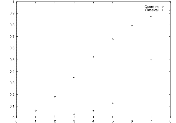
Therefore $\Pr{}_{E}$ tends to one in the limit of large $N$. Here again, in order to compensate for this we have to run the quantum algorithm several times, say $k$ (classically, we would have to sample more and more points). If we want to keep the probability of being “cheated” by an almost–constant function $g$ as low as a given value $\varepsilon$, we evidently have to choose $k$ so that $\left(\Pr{}_{E}\right)^{k}=\varepsilon$, that is

As we would expect, $k$ does tend to infinity in the limit of large $N$, meaning that exploring an even larger domain requires an infinite number of computations. It is nevertheless interesting to study the ratio $\eta=k/N$ of the number of runs to the number of elements in the domain. In the limit of large $N$, this becomes

which is a constant independent on $N$.

Therefore, if we are required to perform the computation with a worst case error probability $\varepsilon$, we have to run our quantum computer a number of times which, in the limit of large $N$, is a definite fraction $\eta$ of $N$. Equation (27) can in this case be inverted to obtain $\varepsilon$ as a function of $\eta$, yielding $\varepsilon=e^{-2\eta}$.

Coming now to the classical case, sampling a fraction $\eta$ of the points in the domain (which requires $k=\eta N$ computations) entails having a probability $\varepsilon=1-\eta$ of mistaking $g$ for $f_{0}$.

In figure 1 we plotted the worst case probability of error against $\eta$ for both the quantum and the classical algorithm in the limit of large $N$. In the quantum case $\varepsilon$ decreases more rapidly and stays well below the classical probability of error as long as $\eta$ is not too close to $1$ (remember that the “sampling” algorithm is no longer probabilistic if we compute our function over its entire domain!).

Looking now at the best case, we find that there is again a single class of functions which is easily dealt with by both algorithms, that is one–to–one functions or permutations of the points in the domain (this obviously requires $N$ to be equal to $M$).

Using the classical sampling algorithm, one can evidently be sure to distinguish an invertible function from a constant one with only two computations, since the former does not assume any value in its range more than once.

In the quantum case, permutations are associated with matrices having exactly one “1” in each row and in each column. Such matrices turn out to be orthogonal to $\mathcal{C}^{\prime}$. Therefore, a measurement of the final state yielded by a permutation can either result in a FAIL or in projection along $\overline{\mathcal{C}}$, which indicates that the function is not constant. Now FAILs can only be obtained with probability $1/N$, which luckily vanishes as $N$ grows larger. We conclude that, in the limit of large $N$, the quantum algorithm is practically guaranteed to spot a one–to–one function at first sight, after a single computation, thus doubling the efficiency of the classical algorithm.

By the way, we note that if we only had to tell constant functions from permutations—if our practical problem didn’t require us to deal with non–invertible, non–constant functions—we would be back to the original situation of Deutsch’s example. We can now see what was so special about the four functions considered by Deutsch in his original example (see equation 2). When both the domain and the range consist of two points only all non–constant functions turn out to be one–to–one, so that all ambiguity is removed.

We are including, in figures 2 through 5, some comparative graphics of the posterior probabilities $\Pr(\mathrm{const}|k)$ expressed by equations (26) and (25) versus the number $k$ of successful computations effected (by successful computation we mean all computations barring FAIL results).

As our previous analysis suggested, the quantum algorithm turns out to be far more efficient than the classical “sampling” algorithm for small values of $k/N$. We emphasize that this result is entirely dependent upon the use of quantum parallelism. This highly non–classical feature of quantum computation apparently allows a quicker exploration of the domain of function $f$, even in the case that the investigated property is not QPC.

The posterior probability $\Pr(\mathrm{const}|k)$ we used for our numerical calculations is conditoned to a sequence of $k$ “constant results” of the quantum algorithm. We have overlooked the possibility of obtaining one or more FAIL outcomes. This is particularly significant when $M=2$ (figures 2 and 3), because in such cases a FAIL result has a $1/2$ probability to show up. This means that in order to obtain $k$ projections of the final state of the computer along $\mathcal{C^{\prime}}$ one must expect to run the quantum computer $2k$ times. Nervertheless, as the graphics show, the quantum strategy always turns out to be convenient, at least for small values of $k/N$.

We finally note that as $N$ and $M$ grow larger (see for instance figure 5) the resulting posterior probabilities turn out to be so low that both the quantum and the classical algorithm are virtually useless. This entirely depends on our assumption of an uniform distribution over functions $f$, which is probably eccessively penalizing. In real–world situations, we can expect the quantum algorithm to be useful in any situation in which the “sampling” algorithm is successfully employed at the present day.

We are grateful to C. M. Becchi for posing the question which led to this work. We acknowledge the interest of G. Castagnoli and the collaboration with Elsag–Bailey; we also thank A. Ekert and C. Macchiavello for interesting discussion. Special thanks to E. Beltrametti for continuous help and advice.

References

- [1] A. Ekert, R. Jozsa: Quantum Computation and Shor’s Factoring Algorithm, Reviews of Modern Physics 68, 733–754 (1996)
- [2] R. Jozsa: Characterizing classes of functions computable by quantum parallelism, Proc. R. Soc. Lond. A (1991) 435, 563–574
- [3] D. Deutsch: Quantum theory, the Church–Turing principle and the universal quantum computer, Proc. R. Soc. Lond. A 400, 97–117 (1985)
- [4] D. Deutsch, R. Jozsa: Rapid solution of problems by quantum computation, Proc. R. Soc. Lond. A (1992) 439, 553–558
- [5] D. R. Simon: On the power of quantum computation, Proceedings of the 35th Annual IEEE Symposium on the Foundations of Computer Science, 1994, 116–123