Stability of 3 Cubic Fixed Point in Two-Coupling-Constant -Theory
Abstract
For an anisotropic euclidean -theory with two interactions the -functions are calculated from five-loop perturbation expansions in dimensions, using the knowledge of the large-order behavior and Borel transformations. For , an infrared stable cubic fixed point for is found, implying that the critical exponents in the magnetic phase transition of real crystals are of the cubic universality class. There were previous indications of the stability based either on lower-loop expansions or on less reliable Padé approximations, but only the evidence presented in this work seems to be sufficently convincing to draw this conclusion.
1 Introduction
The most elegant approach to phase transitions in many physical systems proceeds via field-theoretic renormalization group techniques [1]. The best-studied system is the isotropic Heisenberg ferromagnet with classical spin components. Its critical behavior can be described correctly by an O()-symmetric vector field theory with a quartic interaction .
In a real crystal, such an interaction is never presentably by itself. The crystalline structure gives rise to anisotropies, most prominently of cubic symmetry, which can be represented by an extra field interaction . This term breaks the O()-symmetry by favoring magnetizations along the edges or the diagonals of a hypercube in dimensions. The extended theory interpolates between an O()-symmetric and a cubic system. It has been pointed out a long time ago [2] that, depending on , the O()-symmetric and the cubic fixed point interchange their stability. For , the O()-symmetric, isotropic fixed point is stable. For the isotropy is destabilized and the trajectories of renormalization flow cross over to the cubic fixed point. Estimates using calculations up to three-loops [2]-[4] indicated that must lie somewhere between and . Resummation procedures based on Padé approximations [5] suggested to lie below , thus permitting real crystals to exhibit critical exponents of the cubic universality class. The uncertainty of these estimates have prompted Kleinert and Schulte-Frohlinde [6] to carry the expansions up to five loops. They increased the evidence for considerably, again via Padé resummation.
For a simple -theory, the Padé approximation is known to be inaccurate. At present, the most accurate renormalization group functions for that theory have been obtained by combining perturbation expansions with large-order estimates, using a resummation procedure based on Borel-transformations [7]-[13].
Intending the application of these more powerful resummation methods, the large-order behavior of renormalization group functions has recently been derived for the -vector model with cubic anisotropy, by Kleinert and Thoms [14].
It is the purpose of this letter to combine these large-order results with the five-loop perturbation expansions [6] using a simple Borel-type of resummation algorithm [7, 8], whose power has been exhibited in recent model studies by Kleinert, Thoms and Janke [15].
The results to be presented in this paper allow us to conclude with a reasonable certainty that an infrared-stable cubic fixed point exists at the physically most relevant value . However, due to the vicinity of the isotropic fixed point, the differences in the critical exponents are very hard to measure experimentally. Going beyond the Padé work in Refs. [5] and [6], we also show explicitly the instability and stability of the isotropic and the cubic fixed point, respectively.
2 Resummation
2.1 The Problem
Object of investigation is a -theory with cubic anisotropy. The corresponding energy functional reads:
| (1) |
where is the bare -component field in dimensions, and , are the bare coupling constants. In particular, we shall consider the physically most interesting case of , and continue to . The tensors associated with the two interaction terms in (1) have the following symmetrized form:
The symmetry of the action under reflection and under permutations of the field indices implies the following form of the vertex functions, persisting to all orders in perturbation theory:
| (5) |
| (6) |
The symmetry permits us to renormalize the components of the field and the composite field with only a single renormalization constant and , respectively. The bare field , the composite field , and the two coupling constants and are related to the corresponding physical objects by
| (7) |
where is a mass parameter. We employ dimensional regularization with minimal subtraction. The square brackets around indicate a renormalization of this composite operator. Recall that this renormalization is different from that of the wave function which converts to . In fact it is closely related to the mass renormalization of a theory with mass . In the minimal subtraction scheme, the corresponding renormalization constants are related by: .
The RG-functions are defined in the usual way:
| (8) |
The natural parameter for the anisotropy of the system is the ratio , and the isotropic case corresponds to . We shall use the new couplings and for the calculation of the fixed points from the resummed -functions
| (9) |
The O()-symmetric and cubic fixed points can be obtained by calculating the simultaneous zeros of and . For the physically interesting number of field components, , the infrared-stable cubic fixed point is expected to appear very close to the O()-symmetric one. Since is very small in this region, it will be sufficient to restrict the resummation efforts to the -series accompanying each power , so that the -functions at the cubic fixed point will be approximated by
| (10) | |||||
where indicates resummed -series.
From the five-loop perturbation expansion in Ref. [6], the perturbation coefficients are known up to the order . For and the number of field components , the following expansions are known:
| and | |||||
| (11) |
In addition to the five-loop expansions, the large-order behavior of and has been obtained explicitly in Ref. [14], with the result
| (12) |
The resummation algorithm to be employed in this paper will make use of all these informations.
2.2 The Algorithm
As explained in detail in Ref. [15], it is possible to reexpand a divergent perturbation series
| (13) |
in a special infinite set of Borel summable functions as
| (14) |
so that the approximation
| (15) |
has the same series as up to the powers , while reproducing the known large-order behavior of the perturbation expansion (13).
| (16) |
As shown by Janke and Kleinert in Refs. [7, 8], the natural choice for the functions are certain confluent hypergeometric functions, where for the case of two coupling constants a second index was introduced in Ref. [15]. One possibility was to use
| (17) | |||||
with
| (18) |
Then the coefficients are given by
| (19) |
where are Pochhammer’s symbols. The parameter is free to choose, and may be used to accommodate any strong-coupling power of
| (20) |
if this is known. Since in quantum field theory, this is not the case, will be chosen by the condition of best convergence of the resummed -series in Eq. (15), as explained in the next section.
2.3 Optimal Choice of Strong-Coupling Power
An idea of the relevance of is gained from the study of corresponding models in quantum mechanics, where the strong-coupling behavior can be deduced from scaling arguments. Consider first an O()-symmetric anharmonic oscillator with interaction, where is the number of components of the vector . Here the functions in Eq. (15) represent the resummed ground-state energies . In Figure 1 we have illustrated the convergence of for the anharmonic oscillator with one -component at a coupling constant . We have plotted versus the order of approximation for various values of the strong-coupling parameter . At large , the curves become increasingly independent of and approach a saturation value which coincides with the ground-state energy. This exact result does not depend on . Therefore, we choose the strong-coupling parameter under the condition that the curvature and the slope of the corresponding curve depend minimally on the variation of , when approaching the saturation region. This choice complies with the principle of minimal sensitivity (PMS) which has been used with great success to optimize variational perturbation expansions [16]. Using the discretized form of the first and second derivative, the optimal -value, to be denoted by , is found by calculating the extrema or turning points of the judicial function
| (21) | |||||
where indicates the beginning of the saturation region. In our special example, (see Figure 1.). In Eq. (21) the value of the coupling constant is chosen such that the error of the resummation becomes small and the influence of is isolated. Since the rate of convergence of the resummation decreases for increasing , we determine the optimal at a small coupling constant . In Figure 1., we have plotted the -dependence of for and . The optimal -value is found to be , which is very close to the exactly known strong-coupling parameter .
We mention that for the zero-dimensional case which corresponds to a simple integral with -interaction, the above criterion yields the exact strong-coupling parameter (see Figure 2).
In most applications of quantum field theory, perturbation series are too short to detect the formation of the saturation plateau with sufficient accuracy. We shall see in the following that for shorter series the criterion given above can be simplified without a significant loss of accuracy by neglecting the curvature term in Eq. (21). Then the slope term is deduced from the two highest known partial sums and by forming:
| (22) |
where it is important that and have gotten over the large-fluctuating initial region. Thus the optimal -value, denoted now by , will be determined from calculating the extrema or turning points of . As before, the coupling constant is chosen to be small to ensure a sensitive determination of the optimal .
As the largest available order of approximation for the RG-functions in QFT is , we have plotted in Figure 3 the -dependence of the ratio for the numbers of vector components and at a coupling constant . In the case of , a minimum exists at . For , there is no extremum, and the optimal -value lies at the turning point . In both cases the simplified criterion yields again results for which are close to the exactly known strong-coupling parameter .
It is unnecessary to know to a higher accuracy than that. In order to show this, we have compared the resummed ground-state energies of the anharmonic oscillator using various values of (see Table 1). For the coupling constants and , the rate of convergence to the exact energies depends only very little on .
Consider now the case that in Eq. (13) represents the ground-state energy of the anisotropic quartic oscillator with an interaction
| (23) |
which we have studied in detail in [15] using the Borel-type resummation algorithm of Refs. [7, 8]. When expressed in terms of the old coupling constants , via and , the expression (23) corresponds to the interaction term in the euclidean action (1) for the number of field components . It has been found in [15] that the parameter is the same for each coefficient in the -expansion of the ground-state energy , and having at each the same value as in the isotropic case. The approximation which follows from a resummation of the corresponding perturbation series in up to the order is becoming less accurate for increasing since the -expansions have fewer and fewer terms. However, taking into account the smallness of the anisotropy , the -expansion may be truncated at a finite order . This yields the approximation
which was found to be very accurate in a wide region of around . We have compared the result for the ground-state energy resummed at , which is known from Ref. [15], with the result obtained for . Figure 4 shows the -dependence of the approximated ground-state energy for the two different values of the parameter and various coupling constants . For , the two curves for and coincide. From Figure 4 and Table 1 we can thus conclude that the error which is caused by an inaccurate determination of is negligible.
2.4 Application to Quantum Field Theory
The above analysis of the anisotropic oscillator can now be applied to the corresponding model in quantum field theory. The resummation of the -functions (10) is carried out by combining the formulas (15), (17), and (19), where the function stands now for and . The parameters and follow from the large-order behavior (12), and are the same for both -functions:
| (24) |
The optimal value of the parameter is chosen to cause minimal sensitivity of the ratios and on at the small value of coupling constant [recall Eq. (10)] in accordance with the above observations for the O()-symmetric anharmonic oscillator.
The optimal values are found to be:
| (25) |
For the simultaneous solution of Eqs. (10), we have first determined for each -function all zero-point functions which are implicitly defined by
| (26) |
From the second equation in (10), we have then read off a trivial solution . Restricting attention to the region around the isotropic limit , we have found numerically a second nontrivial solution . For only one solution was found. Having obtained and the isotropic fixed point follows from the condition
| (27) |
The cubic fixed point is similarly obtained by calculating the solution of the equation:
| (28) |
3 Results
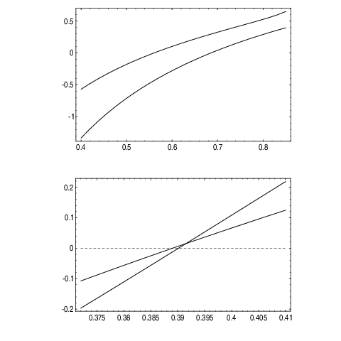
Table 2 contains the numerical values of the isotropic and the cubic fixed points for increasing order of approximation . Starting from the order a cubic fixed point is obtained which lies in the upper half of the plane of coupling constants and . Plotting the functions and , yields the cubic fixed point via the crossing point. This is shown in Figure 5 for the orders of approximation and . The cubic fixed point is found to lie very close to the isotropic one.
In order to convince ourselves of the stability of the cubic fixed point at the number of field components , we calculate the eigenvalues and of the matrix
| (29) |
using the resummed -functions (2.1). The result is contained in Table 3. If both eigenvalues are positive, the corresponding fixed point is infrared stable. For , this is definitely the case for the cubic fixed point. At the isotropic fixed point, one the other hand, one eigenvalue is negative. As the isotropic and the cubic fixed point interchange their stability at , the result corroborate the suggestion in [5] and [6] that the critical value lies below .
Thus we conclude that the critical behavior of magnetic phase transitions in anisotropic crystals with cubic symmetry is governed by the cubic, not by the isotropic Heisenberg fixed point. The corresponding critical exponents and follow from the resummed RG-functions and via the defining relations
| (30) |
Unfortunately, our result is only of fundamental interest and has no easily measurable experimental consequences. Due to the vicinity of the isotropic fixed point, the difference in the critical exponents is smaller than one percent, so that the new cubic universality class is practically indistinguishable from the isotropic class.
References
- [1]
For a review see:
E. Brézin, J. C. le Guillou, J. Zinn-Justin, in Phase Transitions and Critical Phenomena, Vol. 6, eds. C. Domb and M. S. Green, Academic Press, New York (1976);
A. Z. Patashinskii and V. I. Pokrovskii, Fluctuation Theory of Phase Transitions, Pergamon Press, Oxford (1979);
C. Itzykson and M. Drouffe, Statistical Field Theory, Vol. 1 and 2, Cambridge University Press (1989);
D. J. Amit, Field Theory, the Renormalization Group, and Critical Phenomena, World Scientific, Second Edition (1989);
J. Zinn-Justin, Quantum Field Theory and Critical Phenomena, Clarendon Press, Oxford Third Edition (1996). - [2] A. Aharony, Phys. Rev. B 8 (1973) 4270.
- [3] I. J. Ketley and D. J. Wallace, J. Phys. A 6 (1973) 1667.
- [4] E. Brezin, J. C. Le Guillou, and J. Zinn-Justin, Phys. Rev. B 10 (1974) 893; see also: A. Z. Patashinskii and V. I. Pokrovskii, in Ref. [1], Chapter VIII, point 7; I. F. Lyuksvutov, V. I. Pokrovskii and D. E. Khmel’nitskii, Sov. Phys. JETP 42 (1976) 923.
- [5] I. O. Mayer and A. I. Sokolov, Izv. Akad. Nauk SSSR Ser. Fiz. 51 (1987) 2103; I. O. Mayer, A. I. Sokolov, and B. N. Shalayev, Ferroelectrics 95 (1989) 93.
- [6] H. Kleinert and V. Schulte-Frohlinde, Phys. Lett. B 342 (1995) 284.
- [7] For a comprehensive exposition see, W. Janke and H. Kleinert, preprint in preparation.
- [8] W. Janke and H. Kleinert, Resummation of divergent Perturbation Series, World Scientific, Singapore (to be published).
- [9] J. C. Le Guillou and J. Zinn-Justin, Phys. Rev. Lett. 39 (1977) 95.
- [10] J. C. Le Guillou and J. Zinn-Justin, Phys. Rev. B 21 (1980) 3976.
- [11] J. C. Le Guillou and J. Zinn-Justin, J. Physique Lett. 46 (1985) L137.
- [12] J. C. Le Guillou and J. Zinn-Justin, J. Physique 48 (1987) 19.
- [13] J. C. Le Guillou and J. Zinn-Justin, J. Physique 50 (1989) 1365.
- [14] H. Kleinert and S. Thoms, Phys. Rev. D 52 (1995) 5926.
- [15]
H. Kleinert, S. Thoms, and W. Janke,
FU-Berlin preprint 1996 (quant-ph/9605033), Phys. Rev. A (in press). - [16]
H. Kleinert, Path Integrals in Quantum Mechanics,
Statistics and Polymer Physics, World Scientific,
Second Edition (1995);
As an example for the power of this technique see:
W. Janke and H. Kleinert, Phys. Rev. Lett. 75 (1995) 2787; Phys. Lett. A 199 (1995) 287; H. Kleinert and W. Janke, Phys. Lett. A 206 (1995) 283.
F i g u r e C a p t i o n s
Figure 1: Convergence of the ground-state energy of the anharmonic oscillator with . Resummed ground-state energies are plotted versus the order of approximation N for various strong-coupling parameters . The -dependence of the function of Eq. (21). The optimal -value is given by the minimum , very close to the exactly known value .
Figure 2: Judicial function of Eq. (21) to determine the strong-coupling power for the simple integral , plotted as a function of for . The optimal parameter lies at the lowest value of , and is found to be equal to the exact one. It can be shown that for , already the zeroth order of the resummation algorithm used in this paper reproduces the exact value of [8]. This is the origin of the cusp and at .
Figure 3: The -dependence of the ratio in Eq. (22) for the O()-symmetric anharmonic oscillator at constant coupling strength and various numbers of field components . For the simple anharmonic oscillator the optimal -value lies at the minimum. For the two-component oscillator () the optimal value lies at the turning point.
Figure 4: Ground state energy of the anisotropic oscillator with the interacting potential (23), as a function of the anisotropy parameter for two coupling constants and . Comparison is made between the approximation obtained once for the exact strong-coupling parameter and once for . In the case , differences are invisible at this graphical resolution. For comparison, results from another resummation scheme, variational perturbation theory (VPT) [16], obtained in Ref. [15] are shown as well.
Figure 5: Determination of the cubic fixed point , . The nontrivial zeros and of the -functions and are plotted against [see Eqs. (10) and (26)]. The the values of and are found from the intersection point. Up to the order of approximation , no cubic fixed point exist. For the order of approximation , the cubic fixed point is given by , .


| 1 | 0.561496 | 0.56235 | 0.83055 | 0.849631 |
|---|---|---|---|---|
| 2 | 0.558592 | 0.558614 | 0.78297 | 0.784942 |
| 3 | 0.559232 | 0.559254 | 0.812948 | 0.816638 |
| 4 | 0.559142 | 0.559142 | 0.801761 | 0.802012 |
| 5 | 0.559143 | 0.559143 | 0.802206 | 0.802487 |
| 6 | 0.559147 | 0.559147 | 0.805103 | 0.805518 |
| 7 | 0.559146 | 0.559146 | 0.803901 | 0.803937 |
| 8 | 0.559146 | 0.559146 | 0.803115 | 0.803072 |
| 9 | 0.559146 | 0.559146 | 0.803852 | 0.803924 |
| exact | 0.559146 | 0.803770 | ||
| 2 | 0.560616 | 0 | don’t exist | |
| 3 | 0.440796 | 0 | 0.50208 | 0.291074 |
| 4 | 0.393506 | 0 | 0.400199 | 0.037862 |
| 5 | 0.4012 | 0 | 0.411057 | 0.063068 |
| 6 | 0.389037 | 0 | 0.39154 | 0.015309 |
| 4 | 0.782796 | 0.0048920 | 0.784532 | -0.00502046 |
|---|---|---|---|---|
| 5 | 0.764835 | 0.00851725 | 0.763966 | -0.00886277 |
| 6 | 0.80609 | 0.00212717 | 0.80658 | -0.00214788 |