[

]

The real wave functions in association with real Hamiltonians are frequently encountered in numerous physical problems, not to speak of condensed matter physics. There exists still an unresolved problem in defining the Berry phase concerned with the real eigenfunctions in that the gauge potential cannot be defined. The Berry phase [1, 2, 3, 4] arises from a $U(1)$ gauge potential as a result of the adiabatic transition involving the single-valued, complex, non-degenerate eigenstates of a fast subsystem coupled to a slow subsystem. In the following we briefly draw an attention to the main issue of the present work.

In a system described by the time-dependent Hamiltonian $H({\bf R}(t))$ through a slowly varying parameter ${\bf R}$,

the total phase change of the state $|\psi\rangle$ round a closed loop for a time period of $T$ is given by

where the Berry phase $\gamma_{n}(C)$ in the first factor is given by

and $|\psi(0)\rangle=|n;{\bf R}(0)\rangle$ at $t=0$. To obtain a non-zero value of $\gamma_{n}$, the above eigenstate $|n;{\bf R}(t)\rangle$ needs to be single-valued, complex and non-degenerate. Thus one cannot define the gauge potential

from the use of the real eigenfunctions.

In order to allow for the case of multi-valuedness of the complex eigenstates $|n;{\bf R}\rangle$ Berry[1] derived the following expression of the ‘magnetic field’ from (2),

To avoid a confusion found in the literature, once again we stress that $|n;{\bf R}\rangle$ above is the complex (but not real) and multi-valued eigenstate. From this expression one finds the existence of ‘magnetic monopole(s)’ corresponding to the degenerate eigenstates $|m;{\bf R}^{*}\rangle$ at singular point(s), ${\bf R}={\bf R}^{*}$ in the parameter space ${\bf R}$.

The objective of the present study is two-fold; one is to rigorously discuss, in terms of the gauge potential, the Berry phase with the multi-valued real eigenfunctions, and the other, to newly examine the variation of the Berry phase with the strength of electron correlations for a coupled system made of a hole, the fast subsystem, and a phonon, the slow subsystem. In addition, we discuss the two distinctively different cases from which the Berry phase arises; one from a many-body background system and the other from no such background.

As mentioned above, the magnetic field ${\bf B}$ is not definable with the use of the multi-valued real eigenstates $|n;{\bf R}(t)\rangle$, since the gauge potential ${\bf A}({\bf R})$ vanishes. However, by a proper gauge transformation it is possible to define the Berry phase as will be discussed below. The gauge invariance of the equation of motion (1) necessitates the local gauge transformation of the form

The Berry phase $\gamma_{n}(C)$ is then

We now compute the magnetic field ${\bf B}({\bf R})$,

with $m\neq n$ since $\grave{}\langle\nabla_{\!\scriptscriptstyle R}n;{\bf R}|n;{\bf R}\rangle\acute{}\times\grave{}\langle n;{\bf R}|\nabla_{\!\scriptscriptstyle R}|n;{\bf R}\rangle\acute{}$ is a real vector. We find from (1)

The insertion of (8) into (7) and a refinement of its result leads to

Here both $|m;{\bf R}\rangle$ and $|n;{\bf R}\rangle$ are now the real eigenstates unlike the ones in Expression (4). It is important to realize from (7) and (9) that ${\bf A}({\bf R})\neq 0$ but ${\bf B}({\bf R})=0$ at other than the degenerate (singular) point(s) ${\bf R}={\bf R}^{*}$. Thus the Berry phase for the real eigenstates is realized as a type of the Aharonov-Bohm phase.

Let us first examine a one-body problem involving no background. For a particle with spin in the constant magnitude of a magnetic field with slowly varying orientation constrained in the 2-D plane, the Hamiltonian becomes real; $H={{\mbox{\boldmath$\sigma$}}}\cdot{\bf R}=\left(\begin{array}[]{cc}R_{3}&R_{1}\\ R_{1}&-R_{3}\end{array}\right)$ with $\sigma$, the Pauli spin matrix. Choosing $\lambda_{n}(\theta)=nk\theta$ with $k$ being a non-zero integer we write the gauge transformation,

The insertion of (10) into (6) leads to the Berry phase of $\gamma_{n}=-2\pi nk$. The eigenstate of an electron coupled to the magnetic field ${\bf B}$ confined in the 2-D $x$-$z$ plane is real and double-valued. For the double-valued real eigenstates of $|n;\theta\rangle=\left(\begin{array}[]{c}\cos\theta/2\\ \sin\theta/2\end{array}\right)$ with $n=\frac{1}{2}$ as a spin component along the magnetic field, the Berry phase factor round the closed path which encircles $k$ (many) ‘solenoids’ or a single solenoid of strength $k$ is then $\gamma_{n}(C)=-k\pi$. The Berry phase is thus equivalent to the flux in the ‘magnetic solenoid’ with ‘strength’ $-n$ which vertically pierces through the 2-D plane if there exists only one singular point in the plane. In the present case of a particle with no background, the Berry phase is independent of the choice of a path as long as the closed path encircles the solenoids. For the single unit of the solenoid, i.e., $k=1$, the Berry phase factor is $\gamma_{n}(C)=-\pi$ as expected. This is simply an Aharonov-Bohm phase type through the closed path which encloses the single solenoid $k=1$. It is now realized that the geometric phase (Berry phase) with the real eigenstates is composite in nature as it is determined by both the intrinsic property, i.e., the spin of the particle and the magnetic flux of the solenoid. Later we will examine the intrinsic property (spin) of a particle (hole) coupled to a phonon in the many-body background of antiferromagnetic spin correlations. It is now clear that for the real eigenstates $|n;{\bf R}\rangle$ the local gauge transformation $|n;{\bf R}\rangle\acute{}=e^{i\lambda_{n}({\bf R})}|n;{\bf R}\rangle$ is essential for realizing the presence of the gauge potential and the ‘magnetic solenoid’ as in the case of the Aharonov-Bohm phase.

Let $S$ be a simply connected surface bounded by a closed loop in a parameter space ${\bf R}$. If the phase change of the eigenstates $|n;{\bf R}\rangle$ occurs when transported adiabatically round a closed loop on $S$ there must be at least one singular point where $|n;{\bf R}\rangle$ is discontinuous, due to the intersection of potential energy surfaces [4, 5, 6]. In the following we show an interesting case of the Aharonov-Bohm type Berry phase with the choice of a many-body system as a background, in which there can be any number $k$ of singular points through which the ‘magnetic solenoids’ pass vertically through the 2-D plane.

By considering the Holstein-type electron (hole)-phonon coupling [7, 8, 9] we use the effective single-band Holstein-Hubbard model Hamiltonian [10] for a two-dimensional square lattice,

with $n_{i\sigma}=c_{i\sigma}^{\dagger}c_{i\sigma}$. Here the real Hamiltonian $H({\bf R})$ depends on the time-dependent external parameter ${\bf R}$ corresponding to local lattice distortions. $c_{i\sigma}^{\dagger}~(c_{i\sigma})$ is the creation (annihilation) operator of an electron with spin $\sigma$ at site $i$. $t$ represents the electron hopping strength; $U$, the electron-correlation strength; $g$, the electron (hole)-phonon coupling constant and $K$, the spring constant. The local Holstein distortion $R_{i}$ for an in-plane breathing mode at the lattice site $i=(i_{x},i_{y})$ is defined by [11, 12]

where $\Delta_{i}^{x}~(\Delta_{i}^{y})$ is the displacement of oxygen from equilibrium along the positive $x$ ($y$) direction at the lattice site $i$ in the CuO₂ plane and the other two, along the negative $x$ $(y)$ direction as shown in Fig. 1. Unlike the Holstein-$tJ$ model Hamiltonian [11, 12, 13] the Holstein-Hubbard model Hamiltonian [10] above has an advantage of investigating the geometric phase (Berry phase) varying with the strength of correlation in the background.

To obtain the Berry phase for the real ground state wave function, we treat a $4\times 4$ periodic lattice with a hole surrounded by the background of nearly half-filled antiferromagnetic spins. To describe the propagation of the local lattice distortions round a closed path, we write

with $\tau$ being the dimensionless time lapse, $0\leq\tau\leq 1$ between the lattice sites; the lattice distortion (breathing) occurs at site $A$ at $\tau=0$ and at site $B$ at $\tau=1$. In this manner, a closed path in the parameter space ${\bf R}$ can be defined.

The mean field (Hartree-Fock) approximation [14] of (11) is

where the two component spinor is $\psi_{i}=\left(\begin{array}[]{c}c_{i\uparrow}\\ c_{i\downarrow}\end{array}\right)$ and the spin operators are defined by $S_{z}(i)=\frac{1}{2}(c_{i\uparrow}^{\dagger}c_{i\uparrow}-c_{i\downarrow}^{\dagger}c_{i\downarrow})$, $S_{+}(i)=c_{i\uparrow}^{\dagger}c_{i\downarrow}$, $S_{-}(i)=c_{i\downarrow}^{\dagger}c_{i\uparrow}$, and $n(i)=c_{i\uparrow}^{\dagger}c_{i\uparrow}+c_{i\downarrow}^{\dagger}c_{i\downarrow}$.

By minimizing the total energy with respect to the average spin densities $\langle S_{z}(i)\rangle$, $\langle S_{+}(i)\rangle$ and $\langle S_{-}(i)\rangle$, the linearized Hamiltonian (14) was self-consistently treated for the lattice of the periodic $4\times 4$ unit cell. For various values of $U$ and $g$ between $0t$ and $10t$ we evaluated the Berry phase factors. Schüttler et al. [13] employed the Holstein-$tJ$ model by choosing sufficiently strong hole-phonon coupling. Our computed results of the Berry phase factor in the region of strong correlation and large hole-phonon coupling agreed with their results for the case of one-hole tunneling with various paths shown in Fig. 2.

For numerical evaluations of the Berry phase factor we used the path integral approach [3, 13]; the adiabatic quantum transition involving the eigenstate $|n;{\bf R}\rangle$ round a closed path is given by

where the first factor is the dynamic phase factor and the last one, the geometric phase (Berry phase) factor given by

Only for the single-valued complex eigenstates $|n;{\bf R}\rangle$ the Berry phase $\gamma_{n}$ can be obtained directly from the relations (2) and (4). For the real eigenstate with the Hamiltonian (14) we evaluated the adiabatic Berry phase factor (16) by computing the ground state electronic wave functions at each time step $t_{k}$. Lately we [15] found that in scattering processes the role of non-adiabatic intermediate transitions may be important. In such cases, the expression (16) is invalid.

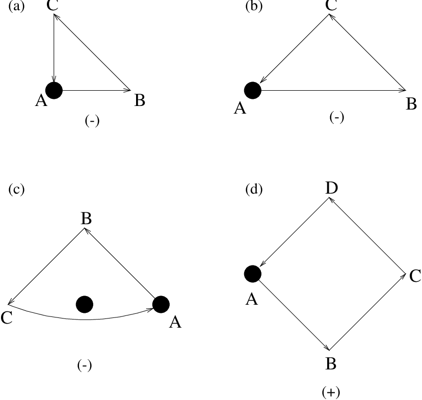
In Fig. 1 a single CuO₄ unit [11, 12] that appears in the CuO₂ planar square lattice of high $T_{c}$ copper-oxide superconductors is drawn to exhibit the local lattice distortions $\Delta_{i}^{x,y}$ involving a copper atom at the center and its four surrounding oxygen atoms. By choosing the strong correlation of $U=6t$ and the electron-phonon coupling of $g=6t$ for various closed paths, the sign of the computed Berry phase factors are shown in Fig. 2. In Fig. 3 we computed each single particle state involving 7 electrons with spin-up and 8 electrons with spin-down respectively for the doping case of one hole with spin-up for the path shown in Fig. 2(b). Due to the limited space we show only the lowest unoccupied energy level denoted as a dotted line for the spin-up electrons. A hole coupled to the local lattice distortion (breathing mode) may move around with some possibility of making a closed loop in the two-dimensional square lattice. A midway point (denoted as $\uparrow$ in Fig. 3) is where a symmetric lattice distortion occurs between two neighboring sites, say, $A$ and $B$. At such midway points the energy gap between the HOMO (the highest occupied molecular orbital) and the LUMO (the lowest unoccupied molecular orbital) is found to be a minimum, indicating that there exist degenerate points in the lattice distortion parameter space $\{R_{i}\}$. The HOMO-LUMO gap becomes a maximum at sites $A$, $B$ and $C$ which correspond to the symmetry breaking points.

In the case of relatively strong electron correlations (large $U$), the computed Berry phase factor was $-1$ for all the triangular closed paths and $+1$ for the closed path of the square shown in Fig. 2. We found that there exists an odd number of degenerate points (singular points), namely 3 of them for the former and an even number of degenerate points, i.e., 4 for the latter. For the case of sufficiently weak correlations, say, $U\leq t$, it is quite interesting to note that the computed Berry phase factor is $+1$ even for the triangular closed paths, contrary to the case of strong correlations. Thus our findings are as follows; the hole behaves as a particle of spin 0 for the background of weak correlations and as a spin $\frac{1}{2}$ fermion for the background of relatively strong correlations. We further found that the Berry phase factor for the hole which behaves as a spin $\frac{1}{2}$ fermion in the background of strong correlations is subject to change its sign depending on the nature of closed paths, i.e., the number of degenerate points that can exist round the closed paths in the parameter space.

The direct use of the multi-valued real eigenstates for defining the ‘magnetic flux’ or the Berry phase is not justifiable. We argued, on the two grounds, the validity of the local gauge transformation $|n;{\bf R}\rangle\acute{}=e^{i\lambda_{n}({\bf R})}|n;{\bf R}\rangle$ with $|n;{\bf R}\rangle$, the real eigenstate; namely the gauge invariance of the equation of motion (1) and the realization of $\lambda_{n}$ as a ‘Aharonov-Bohm’ phase type. In short, using the local gauge transformation we were able to define the ‘magnetic flux’ of a solenoid and thus the Berry phase of the Aharonov-Bohm phase type. We then explored the Berry phase for the adiabatic transitions involving a hole coupled to the lattice distortion (breathing mode) in the antiferromagnetic background of both weakly and strongly correlated electrons.

The following findings are in order. The strength of electron correlations affects the sign of the Berry phase factor; round the simplest triangular closed paths the Berry phase factor of the hole is $+1$ for the case of weak correlation, indicating the hole state of spin 0, and $-1$ for the case of strong correlation, indicating the hole state of spin $\frac{1}{2}$. However the Berry phase factor for the spin $\frac{1}{2}$ fermionic hole depends on the nature of the closed paths, e.g., $-1$ for the triangular closed paths and $+1$ for the square closed path. This is because the sign of the Berry phase factor is determined by the number $k$ of degenerate points (singular points) at which the fluxes pierce through the 2-D plane, depending on the characteristics of closed paths in the parameter space. Thus this is quite different from the system with no background in which the sign of the Berry phase does not depend on the choice of closed paths, as was discussed earlier.

One (S.H.S.S) of the authors is highly grateful to Professor Han-Yong Choi for rendering him an essential part of his current computer code. He acknowledges the financial supports of the Korean Ministry of Education BSRI (1996) and POSTECH/BSRI special programs. He is also grateful to the SRC program (1996) of the Center for Molecular Science at KAIST.

References

- [1] M. V. Berry, Proc. R. Soc. Lond. A 392, 45 (1984)
- [2] B. Simon, Phys. Rev. Lett. 51, 2167 (1983)
- [3] H. Kuratsuji and S. Iida, Prog. Theor. Phys. 74, 439 (1985)
- [4] C. A. Mead and D. G. Truhlar, J. Chem. Phys. 70, 2284 (1979)
- [5] G. Herzberg and H. C. Longuet-Higgins, Disc. Farad. Soc. 35, 77 (1963); H. C. Longuet-Higgins, Proc. R. Soc. Lond. A 344, 147 (1975)
- [6] A. J. Stone, Proc. R. Soc. Lond. A 351, 141 (1976)
- [7] T. Holstein, Ann. Phys. (N.Y.) 8, 325 (1959); 8, 343(1959)
- [8] D. Emin and T. Holstein, Phys. Rev. Lett. 30, 323 (1976)
- [9] J. Hubbard, Proc. Roy. Soc. A 276, 238 (1963); 281, 401 (1964)
- [10] J. Zhong and H.-B. Schüttler, Phys. Rev. Lett. 69, 1600 (1992)
- [11] H. Röder, H. Fehske and H. Büttner, Phys. Rev. B 47, 12420 (1993)
- [12] H. Fehske, H. Röder, A. Mistriotis and H. Büttner, J. Phys.: Condens. Matter 5, 3565 (1993)
- [13] H.-B. Schüttler, K. Yonemitsu and J. Zhong, J. Supercond. 8, 555 (1995); K. Yonemitsu, H.-B. Schüttler, and J. Zhong, unpublished results
- [14] H. Y. Choi, Phys. Rev. B 44, 2609 (1991)
- [15] S.-H. Suck Salk, Phys. Rev. A 53, 2433 (1996)