Decoherence in the dynamical quantum phase transition of the transverse Ising chain

Recently, the dynamics of quantum phase transitions sachdev attracted increasing interest, see, e.g., dziarmaga; cincio+sen; fubini. In contrast to thermal transitions (usually driven by the competition between energy and entropy), they are characterized by a fundamental change of the ground state structure (e.g., from para- to ferro-magnetic) at the critical value of a variable external parameter (e.g., magnetic field). Quantum phase transitions are induced by quantum rather than thermal fluctuations and thus may occur at zero temperature. At the critical point, the energy levels become arbitrarily close and thus the response times diverge (in the continuum limit). Consequently, during the sweep trough such a phase transition by means of a time-dependent external parameter, small external perturbations or internal fluctuations become strongly amplified – leading to many interesting effects, see, e.g., group_phase; vidal; zurek; damski; sengupta. One of them is the anomalously high susceptibility to decoherence (see also fubini): Due to the convergence of the energy levels at the critical point, even low-energy modes of the environment may cause excitations and thus perturb the system. Here, we study the decoherence caused by a small coupling to a rather general reservoir for the quantum Ising chain in a transverse field, which is considered a prototypical example sachdev for a second-order quantum phase transition (and further possesses the advantage of being analytically solvable).

Apart from the general understanding of quantum phase transitions, these investigations are also relevant for quantum computing: By constructing the Hamiltonian appropriately, it is possible to encode the solution to hard computational problems (such a factoring large numbers) in its ground state. In order to reach this solution state, we may start off with a simpler Hamiltonian whose ground state is easy to prepare as the initial configuration. If we now steadily transform it to the problem Hamiltonian, the adiabatic theorem tells us that we stay near the ground state if the evolution is slow enough – and thus finally end up in (or close to) the desired solution state (adiabatic quantum computing farhi; sarandy). However, somewhere on the way from the simple initial configuration to the final state, there is typically a critical point which bears strong similarities to a quantum phase transition (e.g., vanishing gap and diverging entanglement in the continuum limit latorre; gernot). Based on this similarity, it seems gernot that adiabatic quantum algorithms corresponding to second-order quantum phase transitions should be advantageous compared to isolated avoided level crossings (which are analogous to first-order transitions). For an adiabatic quantum algorithm (Grover’s search routine roland) based on a single isolated avoided level crossing markus, the impact of decoherence induced by a low-temperature bath with a well-behaved spectral distribution does not destroy the scalability of the system. However, as we shall see below, the situation may be very different for second-order transitions. These investigations are particularly relevant in view of the recent announcement (see, e.g., dwave) regarding the construction of an adiabatic quantum computer with 16 qubits in the form of a two-dimensional Ising model.

The open system under consideration is described by the total Hamiltonian ${H}$ which can be split up into that of the closed system ${H}_{\rm{sys}}$ and the bath ${H}_{\rm{bath}}$ acting on independent Hilbert spaces ${\mathfrak{H}}_{\rm{sys}}\otimes{\mathfrak{H}}_{\rm{bath}}={\mathfrak{H}}$

plus an interaction $\lambda\,{H}_{\rm{int}}$ between the two, which is supposed to be weak $\lambda\ll 1$ in the sense that it does not perturb the state of the system drastically. Note, however, that the change of the bath caused by the interaction with the system need not be small. In order to describe the evolution of the combined quantum state $|\Phi(t)\rangle\in{\mathfrak{H}}$, we expand it into the instantaneous system energy eigenbasis ${H}_{\rm{sys}}(t)|\Psi_{s}(t)\rangle=E_{s}(t)|\Psi_{s}(t)\rangle$ in ${\mathfrak{H}}_{\rm{sys}}$ via $|\Phi(t)\rangle=\sum_{s}a_{s}(t)|\Psi_{s}(t)\rangle\otimes|\alpha_{s}(t)\rangle$, where $a_{s}$ are the corresponding amplitudes and $|\alpha_{s}\rangle\in{\mathfrak{H}}_{\rm{bath}}$ denote the associated (normalized but not necessary orthogonal) states of the reservoir. Insertion of this expansion into the Schrödinger equation $i|\dot{\Phi}(t)\rangle={H}(t)|\Phi(t)\rangle$ yields ($\hbar=1$)

with the energy gaps $\Delta E_{sr}(t)=E_{s}(t)-E_{r}(t)$ of the system and the total phase (including the Berry phase)

containing the energy shift $H_{\rm{int}}^{sr}=\langle\alpha_{s}|\langle\Psi_{s}|{H}_{\rm{int}}|\Psi_{r}\rangle|\alpha_{r}\rangle$ and $H_{\rm{bath}}^{sr}=\langle\alpha_{s}|{H}_{\rm{bath}}|\alpha_{r}\rangle$. Evidently, there are two contributions for transitions in the Hilbert space ${\mathfrak{H}}_{\rm{sys}}$ of the system: The first term on the right-hand side of Eq. (2) describes the transitions caused by a non-adiabatic evolution (see, e.g., sarandy). Note, however, that the factor $\langle\alpha_{s}|\alpha_{r}\rangle$ and the additional phases in Eq. (3) give rise to extra terms in the adiabatic expansion. The second term in Eq. (2) directly corresponds to transitions caused by the interaction with the bath. Since we are mainly interested in the impact of the coupling to the bath, we shall assume a perfectly adiabatic evolution channels of the system itself $\langle\Psi_{s}|\dot{H}_{\rm{sys}}|\Psi_{r}\rangle\ll\Delta E_{sr}^{2}$ such that the first term in Eq. (2) is negligible and the second one dominates.

The quantum Ising chain of $n$ spins we are going to study exhibits a time-dependent nearest-neighbor interaction $g(t)$ plus transverse field $B(t)=1-g(t)$

where ${\bm{\sigma}}_{j}=(\sigma^{x}_{j},\sigma^{y}_{j},\sigma^{z}_{j})$ are the spin-1/2 Pauli matrices acting on the $j$th qubit and periodic boundary conditions ${\bm{\sigma}}_{n+1}={\bm{\sigma}}_{1}$ are imposed. Choosing $g(0)=0$ and $g(T)=1$ where $T$ is the evolution time, the system evolves from the paramagnetic state $|\rightarrow\rightarrow\rightarrow\dots\rangle$ trough a second-order sachdev quantum phase transition at $g_{\rm cr}=1/2$ to the ferromagnetic phase $|\uparrow\uparrow\uparrow\dots\rangle$ or $|\downarrow\downarrow\downarrow\dots\rangle$.

A major advantage of the above Hamiltonian is that it can be diagonalized exactly sachdev. Let us briefly review the main steps of the diagonalization of ${H}_{\rm{sys}}$, where we switch temporarily to the Heisenberg picture for convenience: The set of $n$ qubits in (4) can be mapped to a system of $n$ spinless fermions $c_{j}$ via the Jordan-Wigner jordan transformation given by $\sigma^{x}_{j}=1-2c_{j}^{{\dagger}}c_{j}$ and $\sigma^{z}_{j}=-(c_{j}^{{\dagger}}+c_{j})\prod_{\ell<j}\sigma^{x}_{\ell}$. In terms of the fermionic operators $c_{j}^{{\dagger}}$ and $c_{j}$, the Hamiltonian assumes a bilinear form containing $(1-g)(1-2c_{j}^{{\dagger}}c_{j})$ and $g(c_{j+1}c_{j}+c_{j+1}^{{\dagger}}c_{j}+c_{j}^{{\dagger}}c_{j+1}+c_{j}^{{\dagger}}c_{j+1}^{{\dagger}})$, i.e., the fermion number $n_{j}=c_{j}^{{\dagger}}c_{j}$ is not conserved in general. This bilinear form can now be diagonalized by a Fourier transformation $c_{j}=\sum_{k}\tilde{c}_{k}\,e^{-ik(ja)}/\sqrt{n}$ followed by a Bogoliubov bogoliubov transformation $\tilde{c}_{k}(t)=u_{k}(t)\,\gamma_{k}+iv_{k}^{*}(t)\,\gamma_{-k}^{{\dagger}}$. Since the new set of fermionic operators $\gamma_{k}$ is supposed to be time-independent, the Bogoliubov coefficients $u_{k}$ and $v_{k}$ must satisfy dziarmaga the equations of motion $i\dot{u}_{k}=-\alpha_{k}u_{k}+\beta_{k}v_{k}$ and $i\dot{v}_{k}=\alpha_{k}v_{k}+\beta_{k}u_{k}$, where $\alpha_{k}(t)=2-4g(t)\cos^{2}(ka/2)$ and $\beta_{k}(t)=2g(t)\sin(ka)$. For an adiabatic evolution $\langle\Psi_{s}|\dot{H}_{\rm{sys}}|\Psi_{r}\rangle\ll\Delta E_{sr}^{2}$, these equations of motion can be solved approximately via $u_{k}(t)\approx[\alpha_{k}(t)+\epsilon_{k}(t)]\exp\{-i\int_{0}^{t}dt^{\prime}\epsilon_{k}(t^{\prime})\}/{\cal N}_{k}(t)$ as well as $v_{k}(t)\approx-\beta_{k}(t)\exp\{-i\int_{0}^{t}dt^{\prime}\epsilon_{k}(t^{\prime})\}/{\cal N}_{k}(t)$ with the normalization ${\cal N}_{k}=\sqrt{2\epsilon_{k}^{2}+2\alpha_{k}\epsilon_{k}}$ ensuring $|u_{k}|^{2}+|v_{k}|^{2}=1$ and the single-particle energies

All the excitation energies $\epsilon_{k}$ assume their minimum values $\epsilon_{k}^{\rm min}=2|\sin(ka/2)|$ at the critical point $g_{\rm cr}=1/2$. In the following, we study the scaling of the involved quantities in the continuum limit $n\uparrow\infty$. In view of the $k$-spectrum $k\in\pi(1+2{\mathbb{Z}})/(an)\;:\;|ka|<\pi$, where $a$ is the lattice spacing, the minimum gap scales as $\Delta E_{\rm min}={\mathcal{O}}(1/n)$. Finally, the Hamiltonian (4) reads

and hence its (instantaneous) ground state contains no fermionic quasi-particles $\forall_{k}{\gamma}_{k}|\Psi_{0}(t)\rangle=0$. Without the environment, the number of fermionic quasi-particles $\gamma_{k}^{{\dagger}}\gamma_{k}$ would be conserved and the system would stay in an eigenstate (e.g., ground state) for an adiabatic evolution.

Of course, the impact of decoherence depends on the properties of the bath and its interaction with the system (decoherence channels). In order to derive generally applicable results, we do not specify the bath ${H}_{\rm{bath}}$ in much detail and start with an interaction $\lambda\,{H}_{\rm{int}}$ which is always present: In the Hamiltonian ${H}_{\rm{sys}}$ in Eq. (4), the transverse field $B(t)=1-g(t)$ appears as a classical control parameter $B_{\rm cl}$. However, the external field $B\to B_{\rm cl}+\delta B$ does also possess (quantum) fluctuations $\delta B$, which couple to the system of Ising spins. Therefore, we start with the following interaction Hamiltonian

where $\delta B$ denotes the reservoir operator. Incidentally, this interaction Hamiltonian yields the same matrix elements as the non-adiabatic corrections $\langle\Psi_{s}|\dot{H}_{\rm{sys}}|\Psi_{r}\rangle$ in Eq. (2), which can therefore be calculated analogously.

Starting in the system’s ground state $a_{0}(t=0)=1$, the excitations $s>0$ caused by the weak interaction $\lambda H_{\rm{int}}$ with the bath $\mathfrak{A}_{s}=a_{s}(T)\exp\{i\varphi_{s}(T)\}$ can be calculated via response theory, i.e., the solution of Eq. (2) to first order in $\lambda\ll 1$ is

We have subsumed all relevant properties of the environment into the spectral function $f(\omega)$ of the bath

where $\Delta\varphi_{s}$ coincides with $\varphi_{s}-\varphi_{0}$ in Eq. (3) apart from the system’s energy gap $\Delta E_{s0}$ and is typically dominated by the contribution from $H_{\rm{bath}}^{ss}-H_{\rm{bath}}^{00}$. As a first approximation, we assume that $f(\omega)$ does not change significantly if we increase the system size $n$ (scaling limit).

After inserting the Jordan-Wigner jordan transformation, the matrix element in Eq. (Decoherence in the dynamical quantum phase transition of the transverse Ising chain) reads

where the $\approx$ sign refers to the adiabatic approximation. Thus, it is only non-vanishing for excited states $|\psi_{s}\rangle$ containing two quasi-particles $s=(k,-k)$ with opposite momenta and hence we get $\Delta E_{s0}=2\epsilon_{k}$. In order to solve the remaining time integrals, it is useful to distinguish different $\omega$-regimes: First of all, in order to have a quantum phase transition (or a working adiabatic quantum computer), the environment should be cold enough to permit the preparation of the system in the initial ground state, i.e., $\omega\ll 2=\epsilon_{k}(t=0)$. For intermediate positive frequencies $2\gg\omega\gg\Delta E_{s0}^{\rm min}\approx 2|ka|$, we may solve the time integral via the saddle-point (or stationary phase) approximation. The saddle-point condition for the exponent in Eq. (Decoherence in the dynamical quantum phase transition of the transverse Ising chain) reads $\omega=\Delta E_{s0}(t_{*})=2\epsilon_{k}(t_{*})$, which corresponds to energy conservation. This condition yields two saddle points shortly before and after the transition $g(t_{*}^{\pm})\approx 1/2\pm\sqrt{\omega^{2}-4k^{2}a^{2}}/8$. For the spectral excitation amplitude $\mathfrak{A}_{s}^{\omega}$ defined via $\mathfrak{A}_{s}=\int d\omega\,f_{s}(\omega)\,\mathfrak{A}_{s}^{\omega}$, the saddle-point approximation yields

Of course, the result depends on the interpolation dynamics $g(t)$, see Table 1. For a constant speed interpolation $g(t)=t/T$, the run-time needed for an adiabatic evolution scales as $T={\mathcal{O}}(n^{2})$ due to the minimum gap $\Delta E_{\rm min}={\mathcal{O}}(1/n)$. For adapted interpolation dynamics $\dot{g}(t)\propto\Delta E(t)$ or $\dot{g}(t)\propto\Delta E^{2}(t)$, however, one may achieve shorter run-times of $T={\mathcal{O}}(n\ln n)$ or $T={\mathcal{O}}(n)$, respectively schaller2006b.

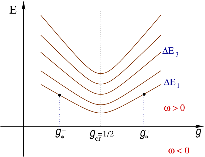
The next (higher-order) terms of the saddle-point expansion scale with ${\mathcal{O}}(\lambda\dot{g}(t_{*})[\omega^{2}-4k^{2}a^{2}]^{-1/2}/\omega)$ and hence the saddle-point approximation breaks down if $\omega$ approaches the minimum gap $\Delta E_{s0}^{\rm min}\approx 2|ka|$, see Fig. 1. In this case, we may obtain an upper bound for the time integral in Eq. (Decoherence in the dynamical quantum phase transition of the transverse Ising chain) via omitting all phases, see Table 1. For frequencies far below $2|ka|$, the saddle points at $g(t_{*}^{\pm})\approx 1/2\pm\sqrt{\omega^{2}-4k^{2}a^{2}}/8$ move away from the real axis and thus the amplitudes are exponentially suppressed in the adiabatic limit

for $g(t)=t/T$ and similarly for the other interpolations. Finally, for negative frequencies $\omega<0$, the saddle points collide with the branch cut generated by the square-root in $\epsilon_{k}$. By deforming the integration contour into the complex plane, it can be shown via an argumentation analogous to schaller2006b that the amplitudes are also exponentially suppressed in this case. This result can be understood in the following way: For frequencies $\omega$ below the lowest excitation energies, the energy $\omega$ of the reservoir modes is not sufficient for exciting the system via energy-conserving transitions. Hence excitations can only occur via non-adiabatic processes for which energy-conservation becomes ill-defined, but these processes are suppressed if the evolution is slow enough.

In summary, we studied the quantum phase transition from paramagnetic to ferromagnetic phase in the quantum Ising chain in a transverse field via its analytical diagonalization and calculated the excitation probabilities channels caused by a weak coupling to a rather general environment (including possible non-perturbative behavior of the reservoir). Since the Ising model is considered sachdev a prototypical example for a second-order quantum phase transition, we expect our results to reflect general features of second-order transitions. For the decoherence channel (7) which is always present (though possibly not the dominant channel), we already found that the total excitation probability increases with system size $n$ (continuum limit): Even though the probability for the lowest excitation $k=\pm\pi/(an)$ can be kept under control for a bath which is well-behaved in the infra-red limit (see also markus), the existence of many excited states $k\in\pi(1+2{\mathbb{Z}})/(an)\;:\;|ka|<\pi$ converging near the critical point causes the growth of the error probability for large systems. This growth can be slowed down a bit via adapted interpolation schemes $g(t)$, but not stopped. Other decoherence channels will display the same general behavior: E.g., for $\omega\gg|ka|$, the associated amplitudes scale as $\mathfrak{A}_{s}^{\omega}={\mathcal{O}}(\lambda\phi_{s}(t_{*})/\sqrt{\dot{g}(t_{*})})$, where $\phi_{s}$ denotes the matrix element in analogy to (10). Typically, for a homogeneous coupling to the bath, $\phi_{s}$ does not strongly depend on the system size $n$ (for given $ka$ and $\omega$). Since $\dot{g}(t_{*})$ decreases for $n\uparrow\infty$ or at least remains constant [for $\dot{g}(t)\propto\Delta E^{2}(t)$], the total excitation probability again increases with system size $n$ few.

Using the analogy between adiabatic quantum algorithms and quantum phase transitions latorre; gernot, this result suggests scalability problems of the corresponding adiabatic quantum algorithm – unless the temperature of the bath stays below the ($n$-dependent) minimum gap childs_robust or the coupling to the bath decreases with increasing $n$. These problems are caused by the accumulation of many levels at the critical point $g=1/2$, which presents the main difference to isolated avoided level crossings (corresponding to first-order phase transitions) discussed earlier markus. It also causes some difficulties for the idea of thermally assisted quantum computation (see, e.g., amin) since, in the presence of too many available levels, the probability of hitting the ground state becomes small.

Therefore, in order to construct a scalable adiabatic quantum algorithm in analogy to the Ising model, suitable error-correction methods will be required. As one possibility, one might exploit the quantum Zeno effect and suppress transitions in the system by constantly measuring the energy, see for example childs_zeno. As another interesting idea, let us study a spatial sweep through the phase transition, i.e., we do not cross the critical point in a homogeneous way, but adopt the following step-wise interpolation: Starting from the initial Hamiltonian $\sigma^{x}_{1}+\sigma^{x}_{2}+\sigma^{x}_{3}+\sigma^{x}_{4}+\dots$, we change it slowly to $\sigma^{z}_{1}\sigma^{z}_{2}+\sigma^{x}_{3}+\sigma^{x}_{4}+\dots$ and afterwards to $\sigma^{z}_{1}\sigma^{z}_{2}+\sigma^{z}_{2}\sigma^{z}_{3}+\sigma^{x}_{4}+\dots$ etc. This corresponds to a nonlinear interpolation path between the two Hamiltonians. In this case, the minimum gap (in the relevant subspace that is even under bit flip) remains independent of the system size $n$ and the run-time $T$ scales linear in $n$ (number of steps). Hence, decoherence could be strongly suppressed for a low-temperature bath. Of course, the generalization of all these concepts and results to more interesting cases such as the (NP-complete) two-dimensional Ising model is highly non-trivial and requires further investigations.

This work was supported by the Emmy-Noether Programme of the German Research Foundation (DFG) under grant SCHU 1557/1-2 and by grant SCHU 1557/2-1.

^∗ email: schuetz@theory.phy.tu-dresden.de

References

- (1)
- (2) S. Sachdev, Quantum Phase transitions, (Cambridge University Press, Cambridge, UK, 1999).
- (3) J. Dziarmaga, Phys. Rev. Lett. 95, 245701 (2005).
- (4) L. Cincio et al., pre-print: cond-mat/0701768 (2007); A. Sen(De), U. Sen and M. Lewenstein, Phys. Rev. A 72, 052319 (2005).
- (5) A. Fubini, G. Falci and A. Osterloh, pre-print: quant-ph/0702014 (2007).
- (6) R. Schützhold et al.,Phys. Rev. Lett. 97, 200601 (2006); R. Schützhold, Phys. Rev. Lett. 95, 135703 (2005).
- (7) G. Vidal et al.,Phys. Rev. Lett. 90, 227902 (2003).
- (8) W. H. Zurek, U. Dorner, and P. Zoller, Phys. Rev. Lett. 95, 105701 (2005).
- (9) B. Damski, Phys. Rev. Lett. 95, 035701 (2005).
- (10) K. Sengupta, S. Powell, and S. Sachdev, Phys. Rev. A 69, 053616 (2004).
- (11) E. Farhi et al., Science 292, 472 (2001); E. Farhi, et al., pre-print: quant-ph/0001106 (2000).
- (12) M. S. Sarandy, L.-A. Wu and D. A. Lidar, Quant. Inf. Proc. 3, 331 (2004).
- (13) J. I. Latorre and R. Orús, Phys. Rev. A 69, 062302 (2004).
- (14) R. Schützhold and G. Schaller, Phys. Rev. A 74, 060304(R) (2006).
- (15) J. Roland and N. J. Cerf, Phys. Rev. A 65, 042308 (2002).
- (16) M. Tiersch and R. Schützhold, pre-print: quant-ph/0608123 (2006).
- (17) IEEE Spectrum online, Tech Talk, February 13th (2007).
- (18) Without the coupling to the environment , the system would stay in its ground state. Thus the only decoherence channel available is heating (i.e., excitations), the phase damping and decay channels, for example, play no major role here.
- (19) G. Schaller, S. Mostame, and R. Schützhold, Phys. Rev. A 73, 062307 (2006).
- (20) A. M. Childs, E. Farhi, and J. Preskill, Phys. Rev. A 65, 012322 (2001).
- (21) P. Jordan and E. Wigner, Z. Phys. 47, 631 (1928).
- (22) E. Lieb et al., Ann. Phys. (N.Y.) 16, 407 (1961); S. Katsura, Phys. Rev. 127, 1508 (1962).
- (23) M. H. S. Amin, Peter J. Love, and C. J. S. Truncik, preprint: cond-mat/0609332.
- (24) If only a few spins are coupled to the environment, the matrix element (for given and ) will generically decrease and then the error probability may be kept under control [for ].
- (25) A. M. Childs et al., Phys. Rev. A 66, 032314 (2002).