Coherent State Distinguishability in Continuous Variable Quantum Cryptography
Abstract
We use the probability of error as a measure of distinguishability between two pure and two mixed symmetric coherent states in the context of continuous variable quantum cryptography. We show that the two mixed symmetric coherent states (in which the various components have the same real part) never give an eavesdropper more information than two pure coherent states.
I Introduction
The security of coherent state continuous variable quantum key distribution (CV-QKD) Wee04; Sil02 is fundamentally based on the inability of an eavesdropper to perfectly distinguish between non-orthogonal quantum states Nie00. In this paper, we look at how much information a potential eavesdropper can gain when trying to distinguish between two pure coherent states as opposed to distinguishing between two mixed coherent states. This is of particular interest in CV-QKD protocols, such as post-selection Sil02), where it is important to determine if an eavesdropper obtained more information in the case of distinguishing between two pure coherent states or distinguishing between two mixed states.
II Probability of Error
In our analysis, we will use the probability of error () measure to distinguish between quantum states. We point out that one could potentially consider other distinguishability measures such as the Kolmogorov distance, the Bhattacharyya coefficient and the Shannon distinguishability (for a review of these measures see Fuc97). However, as we shall see the probability of error measure has a number of useful properties and can be directly calculated for the quantum states we consider in our analysis.
We consider the distinguishability between two general quantum states that are described by the two density matrices and . It was originally shown by Helstrom Hel76 that the probability of error between these two density matrices is minimized by performing an optimal positive operator-valued measure (POVM) Nie00. In this case, the probability of error for the distinguishing between two general quantum states can be expressed as Fuc97
| (1) |
where and are the eigenvalues of the matrix . We note that when the two states are indistinguishable the probability of error is . On the other hand, in the case when the two states are completely distinguishable the probability of error is .

III Distinguishing Pure and Mixed Coherent States
We now look at distinguishing between two coherent states using the previously defined probability of error. A coherent state is defined as where is the displacement operator. It is also a minimum uncertainty state and an eigenstate of the annihilation operator , i.e.
| (2) |
where is the amplitude of the electromagnetic wave Ger05. Any two coherent states and are always non-orthogonal and only approach orthogonality (i.e. ) when where the magnitude is . In the following analysis we will define a coherent state displace in the amplitude and phase quadratures Ger05, by an amount and respectively, as . Consequently, we can write the density operators of two pure coherent states and that we consider here as
| (3) | |||||
In our analysis we also consider two mixed coherent states, i.e. an equally weighted mixture of coherent states mirrored in the phase quadrature and with both mixtures having the same amplitude component. The density operators corresponding to these two mixed states, and , are defined as
| (4) | |||||
Figure (1a) and Fig. (1b) give a two-dimensional phase space illustration of the two pure coherent states and the two mixed coherent states defined by Eq. (2) and Eq. (3) respectively.
According to Eq. (1) we need to determine the eigenvalues of for both the two pure states and two mixed states. To do this we write in its matrix representation which can be expanded in terms of the orthogonal Fock or number states defined as Ger05
| (5) |
where is the creation operator of a harmonic oscillator and . For example, the coherent state written in terms of this Fock basis is
| (6) |
Once is written in matrix form we can then numerically determine its eigenvalues. In this Fock state expansion the inner product of an arbitrary coherent state with a Fock state is given by
| (7) | |||
| (8) |
where and are Fock states. Calculating the general matrix coefficients for the case of the two pure coherent states we obtain
| (9) |
Similarly for the two mixed state case we find
| (10) | |||||
Numerically we calculate the eigenvalues of Eq. (9) and Eq. (10) up to certain values of and . Then according to Eq. (1) this will give us the probability of error in distinguishing between two quantum states. Now having numerically calculated we would like to interpret this in terms of the information gained from using the distinguishing measure.
IV Shannon Information
In the context of CV-QKD it is important to determine how much Shannon information an eavesdropper can obtain by distinguishing between two (pure or mixed) quantum states. The information obtained by distinguishing between two states can be calculated using the Shannon information formula for a binary symmetric channel Sha48
| (11) |
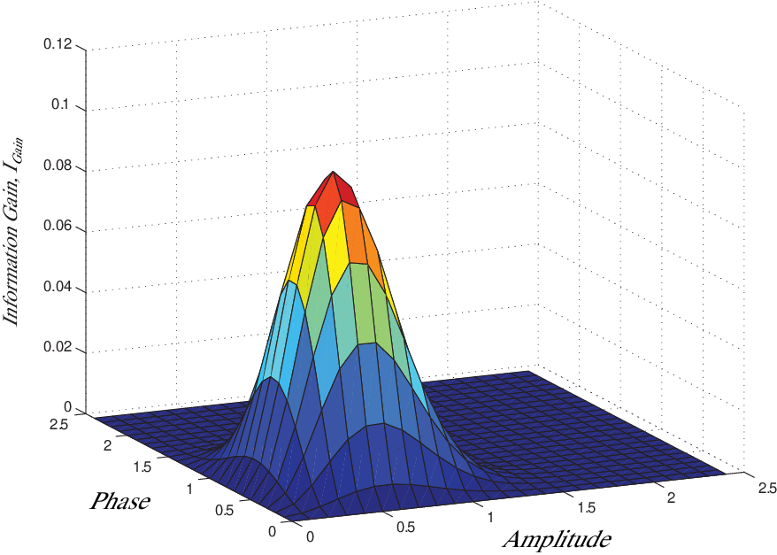
Figure (2) shows the difference between the Shannon information obtained by distinguishing between two coherent states compared with distinguishing between two mixed states . This information difference is defined as . Figure (2) plots in terms of the amplitude and phase quadrature displacements of the pure and mixed states as defined in Eq. (3) and Eq. (4), respectively. Here we have expanded up to Fock states, i.e. in our numerical analysis.
There are two main features of this plot. Firstly, we notice that, given our distinguishability measure and initial configuration of coherent states in phase space, two mixed states never give more information than two pure state, i.e. . Secondly, there is a flat region where the information gain is zero, i.e. the information from distinguishing between two mixed states is the same as that of two pure states. This means as we move the states further and further apart in the amplitude quadrature (while keeping the phase quadrature fixed), the probability of error tends to zero and hence an information gain of zero. The same result occurs when the amplitude quadrature is fixed while varying the phase quadrature. This is somewhat surprising because the more separated two mixed states become the more indistinguishable they are and consequently less information can be extracted. But in this case what it is telling us is that at some point the two mixed states start “behaving” like two pure states.
V Conclusion
In conclusion, we have shown that a continuous variable quantum key distribution protocol where an eavesdropper needs to distinguish between two pure coherent states, rather than two mixed coherent states (where the various mixtures have the same amplitude component), the eavesdropper will never get more information from the two mixed coherent states. We showed this using the probability of error as the distinguishability measure along with the Shannon information formula.
We would like to thank the Australian Research Council for support.
References
- (1) C. Weedbrook et al, Phys. Rev. Lett. 93, 170504 (2004) (and references therein).
- (2) C.Silberhorn et al, Phys. Rev. Lett. 89, 167901 (2002).
- (3) M.A. Nielsen and I.L. Chuang, Quantum Computation and Quantum Information (Cambridge University Press, 2000).
- (4) C.A.Fuchs and J. van de Graaf, IEEE Trans. Info. Theory, 45, 1216 (1999).
- (5) C. W. Helstrom, Quantum Detection and Estimation Theory (Academic, New York, 1976).
- (6) C.C.Gerry and P.L.Knight, Introductory Quantum Optics, Cambridge, (2005).
- (7) C.E. Shannon, Bell Syst. Tech. J. 27, 623 (1948).