Efficient quantum processing
of 3–manifold topological invariants
S Garnerone, A Marzuoli and M Rasetti
†Dipartimento di Fisica, Politecnico di Torino, corso Duca degli Abruzzi 24, 10129 Torino (Italy);
♯ Institute for Scientific Interchange, Villa Gualino, Viale Settimio Severo 75, 10131 Torino (Italy);
‡Dipartimento di Fisica Nucleare e Teorica, Università degli Studi di Pavia and Istituto
Nazionale di Fisica Nucleare, Sezione di Pavia, via A. Bassi 6, 27100 Pavia (Italy)
PACS: 03.67.Lx (Quantum Computation); 11.15.–q (Gauge field theories); 04.60.Kz (Lower dimensional models in Quantum Gravity); 02.10.Kn (Knot theory); 02.20.Uw (Quantum Groups)
MSC: 81P68 (Quantum Computation and Cryptography); 57R56 (Topological Quantum Field Theories); 57M27 (Invariants of knots and –manifolds); 68Q15 (Complexity Classes)
—————————————
(1) silvano.garnerone@polito.it
(2) annalisa.marzuoli@pv.infn.it
(3) mario.rasetti@polito.it
Abstract
A quantum algorithm for approximating efficiently –manifold topological invariants in the framework of Chern–Simons–Witten (CSW) topological quantum field theory at finite values of the coupling constant is provided. The model of computation adopted is the –deformed spin network model viewed as a quantum recognizer in the sense of [1], where each basic unitary transition function can be efficiently processed by a standard quantum circuit.
This achievement is an extension of the algorithm for approximating polynomial invariants of colored oriented links found in [2, 3]. Thus all the significant quantities –partition functions and observables– of quantum CSW theory can be processed efficiently on a quantum computer, reflecting the intrinsic, field–theoretic solvability of such theory at finite .
The paper is supplemented by a critical overview of the basic conceptual tools underlying the construction of quantum invariants of links and –manifolds and connections with algorithmic questions that arise in geometry and quantum gravity models are discussed.
1 Introduction
The possibility of computing quantities of topological or geometric nature was recognized as a major achievement for quantum information theory in a series of paper by Michael Freedman and co–workers [4, 5, 6] (see also [7] for an introduction). Their ‘topological quantum computation’ setting, intrinsically fault–tolerant and protected from decoherence, was designed to comply with the behavior of ‘modular functors’ of Chern–Simons–Witten (CSW) non–abelian topological quantum field theory (TQFT) [8, 9, 10], the gauge group being typically . In physicists’ language, such functors are partition functions and correlators of the quantum theory and, owing to gauge invariance and invariance under diffeomorphisms, which freeze out local degrees of freedom, they share a global, ‘topological’ character. More precisely, the physical observables are associated with topological invariants of knots –the prototype of which is the Jones polynomial [11]– and the generating functional is an invariant of the –dimensional ambient manifold, the Reshetikhin–Turaev–Witten invariant [12, 8].
The search for efficient quantum algorithms to compute
(approximations of) knot invariants has been carried out
by several groups in the last few years.
Within the framework of topological
quantum computation the existence of an
effective procedure has been taken for granted
by resorting to the fact that this model
is polynomially reducible to
the standard quantum circuit model [13].
Later on, this implicit proof has been supported by the fundamental notion
of ‘additive approximation’ introduced in [14] and
borrowed in all the alternative approaches.
The first explicit algorithm for the Jones polynomial
of a knot presented as the plat closure of a braid
has been constructed in [15] by efficiently approximating
unitary matrices associated with a particular representation
of the braid group,
while in [16] the knot presentation
and the representation of the braid group
are generalized (these notions will be
defined in the following sections).
It is worth stressing that both these approaches rely on the standard
model of quantum computation, namely the quantum
circuit model based on qubits, elementary
unitary gates and related algorithmic techniques
such as the so–called Hadamard trick [13].
The approach we proposed in [2, 3]
differs from the previous ones in many respects.
First, we were able to handle more general knot invariants,
namely ‘colored’ link polynomials (a link is a multicomponent knot)
which reduces to Jones’ in a particular case. Secondly, the
model of quantum computation we adopted, that we refer to as the –deformed
spin network model, is in some sense a blending
of the computational schemes mentioned above framed
within the background provided by the theory of
finite–states quantum machines [1].
This topic will be addressed in Section 2, while
a few conceptual questions and implications of our model of computation
will be discussed in the last section of this introduction.
In the main part of the paper, section 3, we extend our efficient algorithm for approximating colored link polynomial to deal with ‘quantum’ –manifold invariants.
In order to overcome the difficulties due to the fact that we shall resort to concepts and definitions arising in many different contexts (low–dimensional topology, quantum group theory, CSW field theory, –dimensional quantum gravity models, classical and quantum complexity theory), we shall illustrate in the next few paragraphs the basic conceptual tools underlying the construction of such ‘universal’ invariants.
1.1 From quantum topology to topological quantum field theory
The term ‘quantum topology’ was introduced by Turaev [17] to denote implications on the topological side of the algebraic theory of quantum groups –technically, deformations of universal enveloping algebras of Lie groups. The latter, based on the pioneering work of Drinfel’d [18] and Jimbo [19], was inspired by theoretical physics from its very beginning since quantum groups and associated –matrix representations are the basic tools of quantum inverse scattering methods and are the backbone of exactly solvable models in statistical mechanics [20].
The deformation parameter was originally assumed to be a real number related to Planck constant by , therefore it is commonly referred to as a ‘quantum’ deformation, while the ‘classical’, undeformed Lie group simmetry is recovered at the particular value (. When dealing with quantum invariants of knots and –manifolds [17, 21] is most often a complex root of unity, the case being considered as the ‘trivial’ one. However, in a topologist’s language, ‘classical’ topological invariants are not the –counterparts of ‘quantum’ invariants, but rather the usual invariants of algebraic and geometric topology, typically related to the fundamental group and homology groups of manifolds and submanifolds.
As Roberts remarks in the introduction to [21] the standard topological invariants were created in order to distinguish between things and, owing to their intrinsic definitions, it is clear what kind of properties they reflect. For instance, the Euler number of a smooth, closed and oriented surface determines completely its topological type and can be defined as , where is the number of handles of . On the other hand, quantum invariants of knots and –manifolds were discovered, but their indirect constuction based on quantum group technology often hides information about the purely topological properties they are able to detect.
What is lost at the topological level is however well paid back by the possibility of bridging this theory with a plenty of issues in pure mathematics and theoretical physics (cfr. the review [21] and the list of references therein). To the early connections mentioned above (quantum inverse scattering, exact solvable models) it is worth adding the operator algebra approach used originally by Jones in defining his knot polynomial [11]. However, the most profitable development of the theory was that suggested by Schwarz and formalized by Witten [8] (see [22] for a review and original references).
Indeed, recognizing quantum invariants as partition functions and vacuum
expectation values of physical observables in
Chern–Simons–Witten
topological quantum field theory provides a ‘physical’ explanation of
their existence and properties. Even more radically, one could speak of a ‘conceptual’
explanation, as far as the topological origin of these invariants keeps on
being unknown. In this wider sense, quantum topology might be thought of
as the mathematical substratum of an CSW topological field theory
quantized according to the path integral prescription (the coupling constant
is constrained to be an integer related to the deformation parameter by ).
The CSW environment provides not only the physical interpretation of quantum
invariants but it does include as well all the historically distinct definitions [23].
In particular, monodromy representations of the braid group [24] appear in
a variety of conformal field theories since point–like ‘particles’ confined in –dimensional
regions evolve along braided worldlines ([25] and references therein).
As a matter of fact, the natural extension of CSW theory
to a –manifold
endowed with a non empty –dimensional boundary
induces on a specific quantized boundary conformal
field theory, namely the
Wess–Zumino–Witten (WZW) theory at level [8, 26].
The latter provides in turn the framework for
dealing with –colored links presented as closures of oriented
braids and associated with Kaul unitary representation of the braid
group [28, 27]. A further extension of this representation
proposed by the same author in [29]
is used in this paper to construct explicitly the quantum –manifold invariants
in the form originally defined in [30] within a purely algebraic setting.
Such quantities are essentially the Reshetikhin–Turaev–Witten
invariants [12] evaluated for –manifolds presented as complements of
knots/links in the –sphere , up to an overall normalization.
1.2 Algorithmic complexity of Chern–Simons–Witten theory
As mentioned in the introductory remarks, the ‘quantum field’ computer [4, 5, 6]
is a model of computation designed to process quantities of topological
nature arising in CSW environment and thus
‘effienciency’ of any calulation –such as that of Jones knot polynomial–
should be guaranteed by definition (we leave aside here the issue of ‘exact’
versus ‘approximate’ calculation at least for the moment).
However, when dealing with algorithmic questions, the
model of computation adopted should comply with the commonly accepted
paradigms of theoretical computer science.
Turing machines, together with the polynomially equivalent
circuit models based on elementary boolean
gates, represent the universal schemes which allow
problems and algorithms to be grouped into classical complexity classes [31].
In quantum computing, the notions of quantum Turing machine –and associated quantum
circuits based on qubits and unitary elementary gates–
can be introduced and represent the standard, universal model
of computation [13].
It was shown in [5] that CSW functors at the fifth root of
unity, whose domain is restricted to
collections of ‘topological’ qubits (disks with three marked points)
on which suitable unitary representations of the braid groups and
act, do reproduce the standard elementary
gates of the quantum circuit model. The physical support of such information processing
consists of anyonic systems obeying particular types of braid statistics, and
work is in progress on the experimental side to check the implementability
of such approach
(see [32] and also [33] for
a different kind of implementation of braiding operators).
Based the above properties, a sort of ‘minimal’ realization
of the full quantum field computer is (polynomially equivalent to) the quantum circuit,
and indeed the work of [15] and [16] on quantum computation of the Jones invariant
does not depend at all on any field theoretic background.
Generally speaking, this
is satisfactory for the aim of introducing an ad hoc
computing model for treating anyonic quantum systems; yet is somehow disturbing
because classical Turing machines and their probabilistic counterparts
are able to simulate efficiently only any dynamical systems governed by classical
laws at any degree of accuracy.
Even the objection that we are in the presence of a quantum field theory
–not simply a quantum mechanical many–body system–
is misleading since the CSW model is exacly solvable at the full quantum level
(for each fixed value of the coupling constant) without resorting to
any approximation such as the low–energy limit [22, 23].
The crucial feature of possessing
only global, purely topological degrees of freedom makes quantum CSW theory
likely to be simulated within a computational scheme based on a discrete
space of states and able to implement polylocal braiding
operations.
As will be illustrated in section 2, the universal model of computation able to handle
all discrete, many–body quantum systems described by (real or virtual)
pure angular momenta states (not simply
two–level systems) as well as solvable field theories
of CSW–type is the (–deformed) spin network proposed in [2, 3].
As already recognized in [4] the task of computing the Jones polynomial of a knot or link represents a major achievement since it is the simplest observable in quantum CSW theory and then its calculation is a testing ground of the effectiveness of topological quantum computation. However, the interest in this algorithmic problem has recently grown in connection with the search for new testing grounds for quantum information theory in general, without necessarily exploiting the physical meaning of the invariant.
The reason why Jones link polynomial is so crucial in the computational context relies on the fact that a ‘simpler’ link invariant, the Alexander–Conway polynomial, can be computed efficiently, while the problem of computing –variable polynomials –such as the HOMFLY invariant– is –hard (see [34, 21, 35] for definitions of these invariants, original references and accounts of algorithmic questions).
The issue of computational complexity of the –variable Jones polynomial in classical information theory can be summarized in
Problem 1
How hard is it to determine the Jones polynomial of a link ?
A quite exhaustive answer has been provided in (JVW), where the evaluation of the Jones polynomial
of an alternating link at a root of unity is shown to be
–hard, namely computationally intractable in a very strong sense.
Recall first that
‘alternating’ links are special instances of links, the planar diagrams of which exhibit
over and under crossings, alternatively. Thus the evaluation of the invariant of generic,
not only alternating links is at least as hard. Secondly, the computation becomes feasible
when the argument of the polynomial is a 2nd, 3rd, 4th, 6th root of unity,
so that the first not easy case involves a 5th root of unity
(refer to [35] for details on this technical issue).
Finally, the complexity class can be defined as the class of enumeration problems
in which the structures that must be counted are recognizable in polynomial time.
A problem in is said to be –complete if for any other problem in
, is polynomial–time reducible to ; if a polynomial time algorithm were found
for any such problem, it would follow that . A problem is –hard
if some –complete problem is polynomial–time reducible to it. Other instances of
–complete problems are the counting of Hamiltonian paths in a graph [31] and the more intractable
problems arising in statistical mechanics, such as the enumeration of all configurations contributing to ground
state partition functions [20].
The computational intractability of Problem 1 does not rules out the possibility of ‘approximating’ efficiently Jones invariant, so that we may ask
Problem 2
How hard is it to approximate the Jones polynomial of a link at a fixed root of unity ( 2nd, 3rd, 4th, 6th root)?
Loosely speaking, the approximation we are speaking about is a number such that, for any choice of a small , the numerical value of , when we substitue in its expression the given value of , differs from by an amount ranging between and (see section 3.2 below for a more precise statement). In the framework of classical complexity theory no algorithm to handle efficiently Problem 2 exists, while the answer in the quantum computational context was given in [14] (see also [16]):
The approximation of the Jones polynomial of a link presented as the closure of a braid at any fixed root of unity is –complete. Moreover, this problem is universal for quantum computation, namely is the ‘prototype’ of all problems efficiently solvable on a quantum computer.
Recall that is the computational complexity class of problems which can be solved in polynomial time by a quantum computer with a probability of success at least for some fixed (bounded) error. In [14] it was proved that , where is defined as the class of languages accepted in polynomial time by a quantum Turing machine with an oracle for the language defined by Problem 2. This equality between computational classes implies that, if we find out an efficient quantum algorithm for Problem 2, then the problem itself is complete for the class , namely each problem in this class can be efficiently reduced to a proper approximate evaluation of the Jones polynomial of a link [16].
Explicit, efficient quantum algorithms for approximating the Jones polynomial
were proposed by Aharonov, Jones and Landau [15] and by Wocjan and Yard [16],
while an early attempt can be found in [36].
In our papers [2, 3] we proved that efficient algorithms can be implemented for
approximating the larger class of ‘colored’ Jones polynomials of links
(addressed also in [37]).
The issue of colored link invariants brings us back to the quantum CSW environment, where they represent the most general gauge invariant physical observables of the theory, being vacuum expectation values of generic Wilson loop operators [8, 22, 23]. In section 3 we shall provide a generalization of our algorithm for colored polynomials to handle the quantum –manifold invariants introduced in 1.1.
Summarizing our results, we have shown that all the significant quantities –partition functions and observables– in quantum CSW theory can be efficiently approximated at finite values of the coupling constant . The intrinsic field–theoretic solvability of CSW theory is thus reflected by its computability on a quantum computer. Looking at the question the other way around, classical computational intractability of Jones and colored polynomials can be viewed as a consequence of their quantum nature. This feature has prevented up to now both exact and approximate efficient calculations of such topological quantities on classical (probabilistic) machines as it happens for simulations of any non trivial ‘genuine’ quantum mechanical system (see e.g. Feynman’s proof in [38]).
1.3 Quantized geometry versus quantum computing
In this section we address some implications of our results
in connection with algorithmic questions that may arise in other physical theories whose
dynamical variables have a geometric character, typically quantum gravity models in
and
spacetime dimensions.
We have however to face preliminarly a conceptual dilemma, namely whether
i) an abstract universal model of computation, able to simulate any discrete quantum system including solvable topological field theories, must exists by its own
or
ii) a (suitably chosen) quantum system is by itself a computing machine whose internal evolution can reproduce the proper dynamics of classes of physical systems.
The second alternative is becoming quite popular thanks to Lloyd’s model, where a net of computing units generates a (superposition of) spacetimes [39] (see also [40] where similar ideas were anticipated).
The idea that many (if not all) aspects of our reality may be thought of as ‘outputs’ of some kind of information processing is both appealing and intriguing. In this connection the role of information theory and its tools is so enhanced that it becomes a unifying paradigm. Of course the classical version of hypothesis i) is usually taken for granted as far as, on the one hand, a (probabilistic) Turing machine is capable of simulating the evolution of any classical system within a given accuracy, and, on the other, all concrete, finite–size realizations of the abstract machine obey the laws of classical physics. The praticability of hypothesis ii) depends heavily on which system is chosen as a simulator and which types of boundary or initial conditions must be imposed to reproduce the dynamical behavior of observed physical systems. Moreover, the concept of ‘efficient’ processing of information seems difficult to be handled without an abstract reference model of computation.
With the previous remarks in mind, we favour assumption i), where the reference model of computation can be represented by the spin network simulator [41, 42, 43] (see also [44]) or its –deformed, finite–size counterpart [2, 3] (see also section 2 below). Note however that it may be tempting to assert that the spin network –thought of as a real net of interacting spin variables– can play as well the role of the reference quantum system in statement ii). This is due to the fact that the recoupling theory of angular momenta –representing the algebraic substratum of the simulator– is the main ingredient of the ‘spin network models’ introduced by Ponzano and Regge [45] and Penrose [46]. Here classical, discretized euclidean geometry arises from recouplings of quantum angular momenta in the asymptotic, large angular momentum limit (see [42], section 5 for a brief account). Thus, much in the sense of ii), spin networks may act –under suitable constraints– as computing machines able to process information encoded into quantum spins to output ‘quantized’ –geometries obeying Einstein equations in the classical limit.
Thinking back to the issue of algorithms for quantum invariants defined in the
framework of quantum CSW theory, our results can be used to test the algorithmic
complexity of quantum gravity models in spacetime dimensions too. This
achievement can be justified –independently from spin network models–
by exploiting the close connection between CSW theory and gravity both
as classical field theories and at the quantum level [8, 26]
(classical gravity with a positive cosmological constant, reinterpreted as
an gauge theory, is quantized through the Euclidean path integral prescription).
For a closed orientable Riemannian –manifold , let
denote the Witten partition function associated with the classical
CS action , being the connection –form. The functional
for finite is the partition function of
Euclidean quantum gravity in the first–order form, where
the coupling constant is related to the cosmological constant by
.
11
1
Note in passing that the invariant ,
on the one hand, equals the Turaev–Viro invariant
for triangulated –manifolds [47] and, on the other, can be derived
by relating gravity to a BF–type topological field theory [8, 22, 26].
The point here is that every manifold in the class considered here can be presented
as the the complement of a link in the –sphere (technically, by surgery
along a framed version of , see section 3.1),
so that
and , where
is the Reshetikhin–Turaev–Witten quantum invariant introduced in 1.1.
Thus the results on algorithms for quantum invariants of links and –manifolds
summarized in 1.2 work equally well in the context of Euclidean
quantum gravity models, reflecting once more the exact solvability of
the theory for finite .
An even more interesting connection between quantum invariants and quantum gravity emerges when dealing with canonical quantization methods applied to general relativity in dimensions. We refer in particular to the ‘loop representation’ based on Ashtekar ‘connection representation’ of canonical gravity (see [48, 49] for reviews and original references). The Reshetikhin–Turaev–Viro invariants act there as quantum states associated with the boundary –geometries (spatial slices of spacetimes). Such states were shown to satisfy both the quantum diffeomorphism constraint and the quantum Hamiltonian constraint (Wheeler–DeWitt equation) once a cut–off –related to the deformation parameter – has been fixed. Thus quantum invariants constitute the natural kinematical arena of loop quantum gravity [50]. This sketchy scenario hides however the necessity of introducing new types of quantum invariants –the perturbative invariants– which arise when the cut–off of the underlying quantum field theory is removed.
In the CSW field–theoretic setting, perturbative invariants emerge as
coefficients of the asymptotic expansion of the partition function
as (see [21], ch. 7). Besides a first term that
corresponds to the semiclassical approximation of (saddle point),
each contribution in the expansion is times a power series in
(here is the CS action evaluated for the flat connection ).
Perturbative invariants are the coefficients of the powers evaluated by using –loop
Feynman diagrams. No complete perturbative treatment of quantum CSW theory is available at present,
and the meaning of such invariants in geometric topology is only conjectured in a few cases.
We are interested here in discussing briefly the ‘volume conjecture’ concerning
special classes of hyperbolic –manifolds (recall that the volume
is a topological invariant for such manifolds). Note also that
most manifolds obtained by surgery on framed links in the
–sphere can be endowed with hyperbolic metrics.
Focusing in particular on ‘hyperbolic knots’, namely
those knots which give rise to finite volume
hyperbolic –manifolds, the volume conjecture proposed
in [51, 52]
(see also the review [21]
for extended versions) can be cast in the form
| (1) |
where is a hyperbolic knot and the notation
stands for the –colored polynomial of evaluated at .
As pointed out many times, all quantum algorithms dealing with link polynomials
are established for a fixed choice of the root of unity appearing in the argument
of the invariants, while the volume
conjecture involves the analysis of the asymptotic behavior of single–colored
polynomials of a same knot for increasing values of the coloring itself.
It would be interesting to explore the possibility of borrowing some of the techniques employed in [53] for dealing with the asymptotics of the Jones polynomial to test conjecture (1) within the computational framework for colored polynomials addressed in the present paper.
Note finally that the relevance of this issue for quantum gravity stems from the observation that all vacuum solutions of Einstein field equations in dimensions with a negative cosmological constant are hyperbolic metrics. As recently shown by Carlip [54], the smallest hyperbolic volumes give rise to the largest contributions in the saddle point term of the path integral of the quantum theory. This implies in turn that the so–called ‘real tunneling geometries’ are most probable (a real tunneling geometry represents the transition from a compact Riemannian spacetime to a Lorentian one within the framework of the Hartle–Hawking ‘no boundary’ approach to quantum cosmology [55]). On the other hand, the possibility of controlling such invariants from the algorithmic point of view might help also in selecting weights to be assigned to –geometries in the ‘sum over topologies’ within a ‘fully quantum’ cosmology theory.
2 Processing braiding operators
2.1 –deformed spin network and quantum recognizers
As pointed out in the introduction, our reference
model of computation to deal with quantum topological invariants
derived from Kaul unitary representations of colored oriented braids [27, 28]
is given by the –deformed spin netwok model.
The (undeformed) spin network simulator has been extensively
addressed elsewhere [42] but for the convenience of the reader
we have collected in appendix A a few mathematical details.
However, in order to
recognize the necessity of introducing a –deformed
version, it is worth to discuss here the (categorical) foundations
of the quantum theory of angular momenta.
The computational space of the spin network simulator
–modelled as a graph– encodes the representation ring
of the Lie group –namely finite–dimensional Hilbert spaces
supporting irreducible representations (irreps) of endowed
with two binary operations, tensor product
and direct sum (that provide a ring
structure over the field )– together
with all the unitary operators relating (multiple tensor products of)
such spaces.
Unlike the usual quantum
circuit model [13], here it is possible to handle directly eigenstates
of binary coupled angular momentum variables labelled by
integers and half–integers (in units) and
not simply –qubit states labelled by the fundamental irrep
. The (re)coupling theory of
angular momenta provides the whole class of unitary transformations that can be
performed on many–body quantum systems described by pure angular
momentum binary coupled sets of eigenstates ([56], topic 12).
The unitaries that we need here
(referred to as –gates in section 3 of [42]) are phase transformations,
related to swaps of two contiguous spins, and
recoupling trasformations expressed in terms of –coefficients of
and related to changes in the interaction schemes of the
angular momenta ().
Within the framework of the categorical approach, the representation ring is an instance of a unitary tensor category, endowed with intertwiner spaces and two basic morphisms, a ‘twist’ (a trivial type of ‘braiding’) and an ‘associator’ [57], [58]. The former acts on the tensor product of two Hilbert spaces supporting irreps of by exchanging the order of the factors, namely
| (2) |
The explicit action of
on a (binary coupled) state is a trivial phase transform, see (62),
(63) in appendix A.
The associator relates different binary bracketing structures
in the triple tensor product of irreps
| (3) |
and is implemented on a binary coupled state as a Racah transform involving one Racah–Wigner –symbol (see (60), (61) in appendix A). Note that both (2) and (3) are isomorphisms (unitary morphisms between intertwiner spaces in the categorical language) but the associator reflects a true (physically measurable) modification of the way in which intertwiner spaces are coupled.
The remarkable fact, derived from the general theory of braided tensor categories [59], is that more complicated multiple tensor products can be handled without introducing any further independent morphism. Actually, multiple tensor product spaces can be related by different combinations of braidings and associators, so that the basic morphisms must satisfy compatibility conditions, a so–called pentagon identity and two exagon identies. In the more concrete language of recoupling theory, each –symbol can be obtained as a combination of phase and Racah transforms and the non–uniqueness of such decomposition is translated into the Biedenharn–Elliott (pentagon) identity and the Racah identity (see e.g. [56] or [60] for their explicit expressions).
In order to deal with non–trivial braiding operators –to be used in connection with the study of braid group representations and braid statistics (typically occuring in anyonic systems)– we are forced to modify the operation in (2) by introducing a genuine, non–trivial braiding morphism [59]
| (4) |
A consistent way of modifying the tensor category to include non–trivial braidings can be achieved by moving to the representation ring of the –deformed Hopf algebra of the Lie group , ( a root of unity). The resulting braided tensor category is the ‘universal’ algebraic structure underlying the constructions of quantum invariants of links and –manifolds outlined in 1.1 and 1.2. (We refer the reader to [2] and to [61] for short technical surveys of the quantum group and CSW approaches.).
According to the above remarks, it should be clear that the ‘–deformed’ spin network model of computation [2, 3] is modelled on the –tensor category
| (5) |
where we have denoted by the –counterpart of the associator in (3). Once suitable basis sets are chosen in the finite collection of irreducible spaces , the unitary morphisms and can be made explicit. In particular turns out to contain the –deformed counterpart of the –symbol and, regarding it as a unitary matrix, it is also referred to as ‘duality’ (or ‘fusion’) matrix borrowing the language of conformal field theories [25].
The efficient quantum algorithm for (approximating) –colored link polynomials we obtained in [3] relies on a two–level procedure which can be summarized as follows.
- •
Kaul unitary representation of colored oriented braids –associated with links presented as plat closures of such braids– is processed on the –spin network (5) in a number of steps that grows polynomially in the size of the input. In particular, each elementary computational step is implemented by applying either or (see section 2.2 below).
- •
The basic –morphisms , in the Kaul representation can be efficiently compiled on a standard quantum computer, by means of universal elementary gates acting on suitable qubit--registers. 22 2 This result is quite interesting by itself as recently pointed out in [62] where relations between the basic morphisms and large Fourier transforms are addressed.
The problem of finding out efficient algorithms to compute the fundamental functions of the quantum theory of angular momenta –Clebsch–Gordan coefficients, –symbols– has attracted much attention [63]. However, to our knowledge, there are neither classical nor quantum algorithms avalaible for evaluating these functions for arbitrary values of their arguments. The crucial remark is that a ––symbol with arbitrary entries can be efficiently compiled and approximated on a quantum circuit independently of the input size of the algorithmic problem owing to the presence of the natural cut–off provided by (see section 3.2, in particular footnote 8). Then we realize once more that the –symmetry of solvable topological field theories is indissolubly tied with the effective computability of these models.
In order to analyze in more details the first topic above we need to frame the –deformed spin network model within the theory of quantum automata and quantum languages. According to [1] a quantum recognizer is a particular type of finite–states quantum machine defined as a 5–tuple , where
- 1.
is a set of basis states, the internal states;
- 2.
is an –dimensional Hilbert space and we shall denote by a start state expressed in the given basis;
- 3.
and are finite alphabets for input and output symbols respectively ( denotes the null symbol);
- 4.
is the subset of transition matrices of the form , where is a unitary matrix which determines the state vector evolution and is a projection operator associated with the output measurement on (suitable complete sets of observables associated with) the upgraded state vector.
In this kind of machine the output alphabet is chosen in such a way that a word written in the input alphabeth must be either accepted or rejected, while for the null symbol the requirement is (the identity matrix). Thus the one–step transition matrices applied to the start state can in principle assume the forms
- a)
,
- b)
with ,
- c)
with ,
according to whether no measure is performed (case a)), or the output is ‘accept’/‘reject’, namely cases b) /c) respectively.
The general axioms stated above can be suitably adapted to make this machine able to recognize a language endowed with a word–probability distribution over the set of words . In particular, for any word the recognizer one–step transition matrix elements are required to be of the form on reading each individual symbol , namely no measurement is performed at the intermediate steps (here run from 1 to , the dimension of the Hilbert space ). Each must satisfy the condition
| (6) |
and the recognizer upgrades the (normalized) initial state to
| (7) |
Then the machine assigns to the word the number
| (8) |
which corresponds to the probability of accepting the word as a whole.
More generally, the machine accepts a word according to an a priori probability distribution with a word–probability treshold if
| (9) |
In what follows the accuracy will be set to , so that the two probability distributions and coincide.
2.2 The Kaul representation as a quantum language
In this section we shall show that
the –deformed spin network computational
scheme (5) embodies
families of quantum finite–states machines
(or quantum automata)
– parametrized by the labels of irreps of
, root of unity–
that recognize the language generated by the
braid group according to a probability
distribution given by the square of the modulus of
the –colored link polynomial.
This construction complies essentially
with what we have done in [2], but
here we should stress the interpretation
of the Kaul representation [28]
as a quantum language, on the one hand,
and the role played by the probability distribution, on the other
(leaving aside details on the field–theoretic background material).
The basic ingredients of Kaul’s construction are oriented geometric braids (see Fig. [1]), the strands of which are endowed with ‘colorings’ given by irreps labels. An –strand colored oriented braid is defined by two sets of assignments with , corresponding to the spin labelling the strand and to the orientation of the strand, with (for the strand going into or away, respectively, from a horizontal rod from which the braid issues). The first set of assignments is associated to the upper rod, the second to the lower rod (we use the convention that two braids are composed in the downward direction). The conjugate of is defined as . It follows that the assignments on the lower rod are just a permutation of the conjugates of the assignments on the upper rod. A colored and oriented braid can thus be represented by the symbol
| (10) |
where for some and and a permutation of .
The composition of two colored oriented braids is well defined only if the orientations and the colors of the two braids match at the merging points, as shown in Fig. [2].

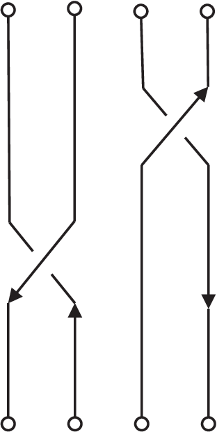
The group of colored oriented braid is generated by the identities (one for each assignment of colors and orientations on a topologically unentangled braid) and by the braids of type , as shown in Fig. [3].

The collection of for are the standard generators of the (colored) braid group and satisfy the following defining relations
| (11) |
The inverse of a generator , ,
corresponds
to the under–crossing of the
left strand in Fig. [3] (right).
In order to obtain a link (multicomponent knot) from a colored braid we
need to ‘close up’ the braid. For our purposes we may consider only the plat closure
(or platting) of a colored braid,
defined for braids which possess an even number of
strands and whose assignments match as follows (see also Fig. [4] )
| (12) |

Since any (colored oriented) link can be obtained as the plat closure of a braid [64], we do not lose generality for what concerns the class of links that can be handled.
The further step consists in embedding the –strand braid into a –sphere with two three–balls removed, giving rise to a –manifold with two boundaries (topologically two -spheres with opposite orientations). The intersections (‘punctures’) of the braid (12) with the boundaries inherit the colorings and orientations from the corresponding strands of the braid (to be associated with Wilson line operators in the ambient CSW topological field theory). Following [8], finite dimensional Hilbert spaces are associated with to the two boundaries , and the basis sets in these spaces are the so–called conformal blocks of the boundary Wess–Zumino–Witten conformal field theory at level , with external lines labelled by (different) irreps of ( is related to CSW coupling constant by , so that from now on we set ). Two particular types of conformal block bases are needed to deal with braids the plat closures of which will give rise to colored oriented links, and their combinatorial patterns are shown in Fig. [5] and Fig. [6].


The (orthonormal) basis sets are constructed by taking particular binary coupling schemes of the ‘incoming’ angular momentum variables which must sum up to give a spin– total singlet state.33 3 Incidentally, such a choice complies also with the conditions necessary for the construction of error avoiding codes and implies as well the robustness of the scheme [65, 66]. The procedure can be carried out by parallelling the , undeformed case (see appendix A) but here the labels of the irreps ’s (integer and half–integers) are constrained to range from to and the binary bracketings on tensor products are decomposed according to rules of representation theory (see e.g. [61], section 3).
Looking at the combinatorial structure of Fig. [5], the most general odd–coupled basis is consistently labelled as
| (13) |
where stands for the ordered string , and . In the even–coupled case depicted in Fig. [6], the states of the basis are denoted by
| (14) |
where is the same as before while and .
The basis vectors associated to the conformal blocks (13) and (14) are related to each other by
| (15) |
where the symbol
represents the unitary duality matrix (or –deformed recoupling coefficient).
As pointed out in section 2.1, it is
a standard result that any such duality matrix can be decomposed into
(sums of) products of ’basic’ duality matrices or – symbols,
see section 3.2 below.
A graphical representation of the decomposition (15) in the case
of eight incoming spin variables is shown in Fig.[7].

Note that the graphical representation of the basic duality transformation (the matrix counterpart of the associator in the language of tensor categories) can be also drawn in the most familiar form shown in Fig. [8].

As proved in [28], the colored polynomial of a link , presented as the plat closure of a colored braid as defined in (12), is given by
| (16) |
where , is the quantum dimension of the irrep labelled by and the quantum integer is defined as
| (17) |
Thus can be evaluated by taking the trace of the matrix elements of the composite braiding operator in the Kaul representation with respect to the odd–coupled basis, where all the intermediate quantum numbers are constrained to give singlet eigenstates (a similar result would hold true for the even–coupled basis).Moreover, can be decomposed into a finite sequence of unitary matrices (diagonal matrices in the odd–coupled basis adopted in (16)) and duality matrices of the type (15) to be applied whenever a switch to the even–coupled basis is needed, namely when an even occurs in the decomposition (see [28] for the explicit expression of these matrices).
The construction outlined above can be cast into an effective
process of calculation by resorting the concept of quantum recognizer
introduced in section 2.1.
The recognizer is defined,
for a fixed root of unity ,
by the 5–tuple
,
where
- •
- •
is the ordered tensor product of –dimensional Hilbert spaces supporting irreps of labelled by , with .
- •
is the braid group on strands whose generators and their inverses represent the input alphabet (we may add the identity element as null symbol).
- •
{ accept, reject, } is the output alphabet.
- •
The transition matrices are expressed in terms of , denoting collectively the Kaul unitary representation matrices, while the projectors are defined as in the general case given in section 2.1.
According to the above definitions, we provide the automaton with an input word of length (written in the alphabeth by natural composition in )
| (18) |
and such that the (plat) closure of the –strand braid gives the link to be processed. Dropping for simplicity all the matrix indices, the unitary evolution of the automaton is achieved by applying the sequence
| (19) |
to a start ket
in the odd–coupled basis (13).
Whenever an odd–braiding (or
) occurs, the
automaton one–step evolution upgrades the internal state
by inserting the eigenvalue of the associated unitary .
On the other hand, when an even–braiding
(or )
must be implemented, the automaton has to change the parity
of the internal state by means of a duality matrix
(15), so that the effective transformation is given by
the product . Since any duality transformation
can be split into a sequence of basic duality matrices, we may look at
the – symbol as representing an ‘elementary’, one–step evolution of
the automaton. By resorting to standard results
in graph theory it is possible to estimate
how many – symbols are needed to decompose the most
general –recoupling coefficient [67], [2]. In the present case
the upper bound can be expressed in terms of , the braid index
(or, equivalently, the number of strands of the input braid).
On the basis of the above remarks, the time complexity
function (number of computational steps) for
processing a braid–word of length
on the quantum recognizer
is bounded from above by [2]
| (20) |
implying that the automaton processes efficiently such braids.
Let us finally comment on the ‘probability distribution’ entering into the definition of a quantum automaton that recognizes a language in a probabilistic sense (end of section 2.1). On the basis of the expression of the colored link invariant given in (16) and by comparison with the word probability of a quantum recognizer defined in (8), it should be quite clear that the probability naturally associated with a link processed on is the square modulus of its colored polynomial (note that the positivity conditions required in (6) are always satisfied).
In order to check this result in a concrete case, the explicit construction of the –spin network automaton that recognizes the braid group language with a probability distribution given by the square modulus of the Jones polynomial is carried out in appendix B.
3 Efficient quantum algorithms for –manifold
quantum invariants
3.1 Colored framed links and 3–manifold quantum invariants
The quantum invariants of –manifolds that we are going to discuss –within the mathematical framework developed in [30], see also [68]– can be obtained as combinations of polynomial invariants of ‘framed’ unoriented links in the –sphere on the basis of theorem 1 stated below. It is worth noting that in the CSW environment the necessity of introducing framings is physically motivated by the requirement of general covariance of the quantized field theory (see e.g. ch. 3 of [23]).
Loosely speaking, a framed oriented link is obtained from a link –thought of as made of knotted strings– by thickening its strings to get oriented ‘ribbons’. If has knot components , for each we introduce another closed path oriented in the same way as and lying within an infinitesimal neighborhood of (knots and links are embedded in or in ). The overall topology of the link is not modified, but for each we now have an extra variable telling us how many times the oriented ribbon is ‘twisted’. Denoting by the framing of the link , is the self–linking number of the band, or equivalently the linking number between the knot and its framing curve which winds times in the right–handed direction. The twist of the band is not independent from , and the simplest choice we can made is to set
where is the writhe of the --th component.
44
4
Given a link diagram , namely a projection of the oriented link
onto a plane, we can define two numerical invariants associated with such diagrams.
The writhe number is given by
where are the crossing points and
according to whether there appears an over–crossing of the left strand over the right strand
or an under–crossing (both strands are oriented upward).
The linking number, defined for a link with more than one component knot,
is defined for each pair of components as .
It can be shown that the writhe is a regular isotopy invariant
for knots and link and the linking number is an ambient isotopy invariant for links.
Recall that two links in (or ) are ambient isotopic if they can be
continuously deformed one into the other. It can be shown that
two links are ambient isotopic if and only if their diagrams
are connected by a finite sequence of Reidemeister moves of
type I, II, II. Regular isotopy is a restricted
type of equivalence among links where the allowed
Reidemeister moves are of type II and III. It is worth noting that
the colored link polynomials (16) are invariants of
regular isotopy while an associated ambient isotopy invariant can
be obtained by multiplying by
, where is the writhe
defined above.

The type of framing usually adopted is the ‘vertical’ framing, where the frame is thought to be placed vertically above the link diagram. Looking at Fig. [9], the framing can be represented by putting the writhe number nearby the band or even by writing next to the string representing (a portion of) .
The –manifolds we are going to consider are closed, connected and oriented,
namely compact and without boundary. In general any such manifold
can be presented as the union of several components
–endowed with –dimensional boundaries–
glued together by suitable identification prescriptions on the
points lying in their boundaries. If the components are sewed together in
a different way a topologically different manifold
may be obtained (recall that two manifolds are topologically equivalent
iff they are homeomorphic, namely there exists a one–to–one
continuous map between them). The new
manifold
is said to be obtained from by means of ‘surgery’.
The fundamental theorem that
characterizes (equivalence classes of homeomorphic) –manifolds
reads [69, 70]
Theorem 1. Every closed, connected and orientable –manifold can be obtained by surgery on an unoriented framed link in the –sphere .
Following [23], let us illustrate in some details
the (Dehn) surgery procedure referred to in the statement of the theorem
in the simple case of a knot (–component link) .
The building blocks of the construction are solid tori, so let us
begin the discussion by considering
the –dimensional torus
(the cartesian product of two unit circles).
A point in can be specified by the
coordinates in
the complex plane and in particular
a point lying on the longitude has coordinate while
a point in a meridian has coordinate .
A solid torus is a –manifold
homeomorphic to , where
is the –dimensional disc. The boundary
of is the torus
.
A framing on the solid turus is a particular
homeomorphism .
Given a framing of ,
is a meridian while is a longitude.
A tubular neighborhood of a knot in
is an embedding
such that .
The framing of a knot
is defined as the framing of the tubular neighborhood of the
knot. In particular, the standard framing of a
knot is such that the linking number is
equal to zero.
Representing the unit disc in the complex plane,
the points of have coordinates
with .
The self–homeomorphisms of ,
defined explicitly by
| (21) |
are the basic twist operations of .
Given a tubular neighborhood of a knot
with standard framing ,
the right–handed and left–handed twist of
are related to the by
| (22) |
A Dehn surgery performed along a (framed) knot can be described as follows.
- 1.
remove the interior of a tubular neighborhood of (the resulting manifold is the complement torus);
- 2.
consider and as distinct spaces;
- 3.
glue back and by identifying the points in their boundaries through a given homeomorphism .
The resulting manifold is recovered by setting
| (23) |
and it is completely specified by the knot and by the chioce of the gluing homomorphism . Equivalently, the surgery is characterized by the knot and by a closed curve representing , where is the meridian of .
Dehn surgery is a simple and constructive prescription which basically consists in removing and sewing back solid tori from the –sphere. However, since different surgery instructions may give rise to homeomorphic manifolds, it is crucial to define the equivalence relations that identify the surgery instructions providing the same (homeomorphism class of) –manifold. Once these rules are taken into account, the classification problem for –manifolds can be actually reduced to the problem of classification of knots (links).
The equivalence relations among
surgery instructions yielding a same –manifold
are topological operations on framed link diagrams known as
Kirby moves.
I move. The configuration described by the unknot
, with framing , enclosing
unlinked strands , with framing ,
lying on a ribbon
can be changed into the configuration where
is removed and the ribbon is twisted in the clockwise
direction from below, see Fig. [10]. The framing
of the components ’s must be changed
according to
| (24) |
where is the square of the linking number between and .

II move. An unknotted link with framing can be removed without affecting the rest of the link, see Fig. [11];

III move. This is the ‘inverse’ of the first move and amounts to change the configuration containing with framing into the anti–clockwise twisted ribbon of ’s and without . Here the framings change according to
| (25) |
IV move. This is the ‘inverse’ of the second move. An unknotted link with framing can be removed without affecting the rest of the link.
The extension of the results stated above in order to deal with –colored surgery links to be associated with –manifold invariants can be carried in a quite straightforward way. The construction developed in [2, 3] and summarized in section 2.3 basically relies on Kaul unitary representation of (colored) oriented braids on strands [28] and thus we need preliminarly to generalize such a representation to deal with unoriented braids and links. The goal can be achieved by suitably modifying the eigenvalues of the elementary braiding matrices in the odd–coupled basis introduced in (13) according to [29]
| (26) |
where and are the quadratic Casimir
invariants associated with the irreps .
The in the exponent of the parameter refer to left–handed
(respectively, right–handed) half–twists in two parallel strands carrying the coloring
and it can be easily checked that these eigenvalues
do not depend on the orientations but only on the over/under–crossing features
(the colored strands are ordered from left to right
as happened for oriented braids, see (10) and Fig. [3]).
It is worth noting that the duality matrices (15) –needed
whenever an even braiding has
to be applied– are independent from orientations of the strands,
so that they can be used in the present context with no further modification.
According to Theorem 1, what we really have to handle are colored links in the vertical framing and then the effect of adding or deleting a in the writhe of the link must be properly taken into account (this operation in the standard framing would not affect the topology of the link). Referring in particular to a –colored framed unknot , the associated link invariant turns out to be changed into
| (27) |
where on the left–handed sides
denote the vertical framing while in the right–handed sides
there appears the knot invariant of the unknot in the standard –framing, whose numerical
value is given by the –dimension
defined in (17). The latter
relations provide in practice the operatorial
content of Kirby moves applied to framed colored links.
Then the requirement of invariance under Kirby moves of the
forthcoming –manifold topological invariants makes it necessary to
compensate the effects of (3.1) by resorting to
properties of the so–called linking matrix.
For a framed link whose components
have framings respectively,
the linking matrix is a symmetric matrix defined as
| (28) |
where is the linking
number between the component knots and .
The signature of the linking matrix, denoted by ,
is the difference between the
number of positive and negative eigenvalues of .
With these preliminary definitions, let us state the following theorem,
the original proof of which can be found in [12, 30] (see also [68]).
Theorem 2. For a closed, connected and oriented –manifold obtained by surgery in the –sphere along an unoriented colored framed link with link components and for any fixed root of unity the quantity
(29) is a topological invariant of the –manifold endowed with the framing assignment .55 5 This means in practice that, on applying Kirby moves I-IV to , the value of the invariant does not change, namely depends only on the homeomorphism class of the –manifold. Note however that we are not in the presence of a complete –manifold invariant since there exist topologically distinct manifolds with the same .
The extension of the theorem to deal with surgery operations performed on manifolds topologically different from and to situations in which –deformations of other semisimple Lie groups are involved can be found in the reference quoted above. All such invariants are collectively referred to as –manifold ‘quantum invariants’ or even as ‘state sum models’ by noticing that an expression like (29) can be interpreted as a partition function over suitably weighted ‘states’ represented by the link polynomials with different colorings.
Here , , run over and the summation is performed over all admissible colorings. in the previous expression is the ‘unoriented’ counterpart of the polynomial for the link with coloring assignment on its components and the summation is performed over all admissible colorings.
It is worth noting that the presentation of the colored links
used both in section 2.2 (see (16)) and in (26)
is slightly different from the presentation
given in Theorem 2 above, even
though we keep on using the same notation for the colorings.
In the latter case a coloring is assigned to each of the link components,
while in the former we label the strands of the associated braid
with colors (see e.g. Fig. [4]).
However, what really matters is the fact that both
presentations of the link give rise to the same invariant,
as could be proved by exploiting the properties
of the –representation ring.
From the computational viewpoint this
twofold choice does not matter
as well because we could efficiently implement
the transformation from a given link diagram to any
associated closed braid on a classical computer
(see e.g. section 2 of [61] for a discussion
on classical algorithmic questions about braids and links).
Expression (29)
makes it manifest the overall dependence on the framing in the factor
,
but in what follows we are going to express the link
polynomials
as expectation values of Kaul unitary representation [29]
worked out for an unoriented –strands braid the
plat closure of which gives the link under examination.
3.2 Quantum algorithm for approximating –manifold invariants
In this section we shall describe the quantum algorithm for computing the colored polynomial and the associate invariant defined in (29). This algorithm is an extension of the quantum algorithm proposed in [2, 3] which efficiently approximated the value of the colored Jones polynomials (16).
As anticipated in section 1.2 we need in the present context the notion of additive approximation introduced [14] (see also [16]). Given a normalized function , where denotes an instance of the problem, we have an additive approximation of its value for each if we can associate with a random variable such that
| (30) |
for any . Moreover, the time needed to achieve the approximation must be polynomial in the size of the problem and in . Then the problem we are interested in can be stated formally as follows.
Approximating –manifold invariants.
Given a framed link with component knots , framing , a positive integer , and a set of allowed colors , we want to sample out a random variable –representing an additive approximation of the value of the normalized –manifold invariant evaluated at – in such a way that the following condition holds true
(31) The size of the problem is expressed in terms of the number of crossings of the surgery link and by the number of strands of the associate braid, (as it happened for colored link polynomials), but we shall need to handle properly the whole set of allowed colorings and the framing as well.66 6 From now on we agree that the invariant is normalized by the product of the –dimensions associated with the link components, namely by the factor .
As anticipated in section 2.1, the quantum algorithms for evaluating (additive approximations of) topological invariants in the framework of quantum CSW theory are based on a two–level procedure outlined already in [3] in connection with colored link polynomials and improved here for –manifold invariants. The rationale underlying our procedure is briefly summarized below while technical details are developed in the rest of the section.
- (A)
Within the computational model of the –deformed spin network recognizer (section 2) both topological and field–theoretic data –encoded into a framed colored link associated with a unitary braiding operator in the Kaul representation [29]– are efficiently processed. The estimate of the time complexity function (number of computational steps) required to complete the calculation given in (20) still holds true.
- (B)
By resorting to standard quantum circuit model techniques and related approximation schemes it can be shown that
- a)
the start state of the recognizer needed for processing the –manifold invariant is efficiently encoded into a qubit register;
- b)
the braiding operator associated with the framed link –already split into a sequence of ‘elementary’ braiding and duality transformations on the basis of the recognizer design– can be efficiently compiled on a standard quantum circuit applied to the start qubit register;
- c)
by resorting to the Hadamard test [15] –an efficient sampling procedure which provides the expectation value of an unitary operator on a (qubit) state– it is possible to estimate the value of the invariant from a series of measurements on an ancilla qubit coupled to the start state.
This two–level computational process for the approximation of –manifold invariants in the sense of (31) is thus efficient with respect to the standard model of quantum computation and not simply from the viewpoint of the –deformed automaton model.
- a)
- (C)
The expectation value of the braiding operator evaluated on the start state and sampled as described above, can in turn be related to a suitable probability distribution on the language(s) recognized by . In view of the properties of such distributions (cfr. the concluding remarks of sections 2.1 and 2.2 and appendix B), the whole procedure can be reinterpreted by saying that the automaton recognizes the language of the braid group with a probability distribution given by the square modulus of the (normalized) invariant .
Given an unoriented link presented as the plat closure of a –strands
braid with a fixed set of colorings (see section 2.2 for the oriented case,
in particular Fig. [4]), let us denote again the conformal block odd–coupled basis
of the boundary WZW theory by as in (13)
and Fig. [5].
Here
and
and both and the intermediate quantum numbers
take values in the collection , bounded form
above by the coupling constant of quantum CSW theory.
Each spin quantum number can be encoded into a qubit register made of
qubits, where
denotes the smallest integer
, see Fig. [12].

Since an element of the basis is specified by quantum numbers (j,p and r), we need
| (32) |
qubits to encode one basis vector. The ordering on such quantum register is shown in Fig. [13], where the three sets of quantum numbers are associated with a j–register, a p–register and a r–register respectively.

The unitary braiding operator associated with the –strands unoriented braid
under consideration can be decomposed –following the scheme explained
in section 2.2 and updating the representation according to [29]–
into ‘elementary’ odd braidings and duality trasformation.
The elementary braiding matrices are diagonal in the odd–coupled basis,
so that their action can be easily implemented on the quantum register
of Fig. [13]. The quantum
gate realization of is simply the
identity matrix on the –registers,
while the –register is modified by the action
of a SWAP gate and a phase gate with a phase factor given by
the eigenvalue in equation (26).77
7
Recall that a SWAP
acting on two qubits , is the operation
which corresponds to the matrix

The duality transformation introduced formally in (15) must be applied whenever an even elementary braiding matrix is encountered in order to recover the current, odd–coupled basis. The associated (–deformed) coefficient can be split into a sequence of ‘elementary’ duality transformations according to
(see Fig. [7]
of section 2.2 for the graphical representation of such decomposition).
Each symbol in the latter expression is the matrix form of a –
coefficient (see Fig. [8]), namely
| (46) |
where the labels of the quantum numbers has been slightly changed to comply with the following standard explicit expression of the –
The symbols are combinatorial factors involving
the factorials of –dimensions (see appendix I of [28]),
where the factorial of a –number is defined as
.
For each choice of the entries (in the allowed set
)
the latter power series is actually a summation over the finite set of (integer and half–integers)
’s that yields non–negative quantum integers.
From the remarks above it should be clear that the problem of efficiently
implementing (3.2), namely the most general change of basis,
is equivalent to the simpler problem of efficiently
compiling a sequence of – symbols or elementary duality matrices
(46). But any such coefficient (i.e. the symbol
with a fixed set of entries) can be easily and efficiently evaluated with
a classical computer owing to the finiteness of its explicit expression
(3.2).
On the other hand, it is necessary to make explicit the
action of the matrix (46) on the qubit register, namely
on an Hilbert space of dimension
for each admissible set of entries.
88
8
The ‘classical’ –symbol can be expressed in terms of
a series similar to (3.2), but the encoding
of such symbols on qubit registers would depend explicitly on the values of the entries,
so that the computation is not obvioulsy efficient with respect
to the size of the input data, see footnote 2 in section 2.1.

The circuit realization is shown in Fig. [15], where the j–register acts as a control register on the qubits of the p(r)–registers involved in the transformation. The transformation can then be thought of as a gate with a ‘block structure’, or a multiplexor associated with the block structure depicted in Fig. [16]. Each block corresponds to a particular configuration of the j–qubits, and the matrix element inside the block are –, up to suitable factors (equation (46)).
On the basis of the decomposition in (3.2) we realize that the allowed elementary duality matrices are always parametrized by the set of those quantum numbers which remain unchanged when they are applied to the proper registers. The crucial remark here consists in noticing that the dimension of these matrices is independent of the size of the problem, determined by the index of the braid group and the number of crossings. Since there exist efficient methods to approximate unitary matrices of a given dimension [71], a sequence of universal gates can be always worked out that efficiently approximate every – as well (see [72] for more details).

The number of elementary duality transformations needed to decompose a general duality transformation (7) is , linear in the size of the problem under consideration. The action of a – recoupling transformation on the register of Fig. [13] is shown in Fig. [17]. Note however that, once all the gates represented by – have been applied, it is necessary to swap some of the qubits in order to recover the proper order in the register, see Fig. [18].


Upon applying a – recoupling transformation we end up in
the even–coupled basis
(see (14) and Fig. [6]) which
diagonalizes the even braiding matrices
of the Kaul representation. Their action on the (even) qubit register can then be implemented
by paralleling the procedure described in the odd case.
The further step consists in going back to the
basis, which can be achieved by means of the finite sequence of
– transformations shown in Fig. [19],
eventually completed by a suitable sequence of SWAPS to recover the
initial ordering of the start register.

This completes the analysis of the quantum circuit which implements efficiently the Kaul representation [29] on the Hilbert space spanned by the odd–coupled basis of conformal blocks (point b) at the beginning of this section).
For what concerns the preparation of the start state according to point a), notice once more that we have considered so far the case of an unoriented link (plat closure of a –strands braid) with a fixed coloring set . As already pointed out in the case of oriented links (see section 2.2, (16) and appendix B) the start state of the automaton calculation is a singlet vector in the odd–coupled basis
| (51) |
which can be efficiently encoded into the qubit register of Fig. [13] as a particular case of the construction carried out above. Then the polynomial for an unoriented, framed link can be recovered as the (trace of the) expectation value of the associated braiding operator in the updated Kaul representation. However, the start state of the recognizer needed for processing the –manifold invariant must be prepared in order to comply with the summation over the colorings in (29). The goal can be achieved in a quite staightforward way by resorting to quantum parallelism, as described in the following.
As before, we first split the qubit register into three ordered parts, the j-, p– and r–registers. Then we initialize the j–register into the following weighted superposition of states
| (52) |
with ( in the number of link components and the coefficients ’s are defined as in Theorem 2 of section 3.1). Since the link can be considered as the plat closure of a braid word , the quantum circuit needed to encode the start state can be implemented by the following composition of unitary gates
| (53) |
where is the SWAP gate on the j–register and is the state obtained from the application of the circuit .
The following sequence of equalities shows that this quantum circuit actually gives the required –manifold invariant
| (54) | |||||
Recall that the signature of the linking matrix can be easily computed classically once the linking matrix (28) (which is part of the topological input data of the algorithmic problem) is given.
4 Concluding remarks
We have shown that all the significant quantities –partition functions and
observables– in quantum CSW theory can be efficiently approximated
by quantum algorithms at finite values of the
coupling constant , reflecting the intrinsic field–theoretic solvability of this theory.
The efficiency of the quantum algorithms is proved on the basis of a two–level
computational scheme which relies on the implementation of unitary representations of the braid group
proposed in [28, 29]. In particular, as shown in section 3.2, the representation needed
to handle –manifold quantum invariants can be efficiently compiled on
a quantum circuit equipped with a suitable start qubit register,
namely within the ‘standard’ model of quantum computation.
The relevance of our result in connection with the algorithmic complexity of quantum CSW
theory has been extensively addressed in section 1.2, while further developments and
applications to geometry and quantum gravity models had already been discussed in 1.3.
More generally, it would be interesting to improve our approach, on the one hand,
by handling quantum topological invariants arising from CSW theories
with arbitrary semi–simple Lie
groups [73] and, on the other,
by exploring the quantum computational complexity
of solvable models in statistical mechanics [74].
Finally, let us comment in some more details the issue concerning the model of quantum computation adopted . As pointed out in (A) and (C) of section 3.2, a central role in our procedure is played by the quantum recognizer able to process efficiently the language generate by the braid group with transition matrices given by Kaul unitary representations (section 2.2 and 3.2) and probability distributions associated with quantum topological invariants. It may be tempting to proceed without this step, processing directly the unitary representations within the quantum circuit scheme of computation. However, we proved in section 3.2 that the basic morphisms of the –tensor category on which the recognizer is modelled can be efficiently compiled and approximated on a quantum circuit (in particular the implementation of a – transformation is independent of both the input size of the algorithmic problem and on the values of its entries; see also footnotes 2, section 2.1 and 8, section 3.2).
This achievement, quite remarkable as it is by itself, opens as well the further possibility of looking at the –spin network simulator as the fundamental model of computation for a wide range of algorithmic problems in geometric topology and group theory. According to the quantum recognizer definition given in section 2.1, the specific problems that can be dealt with it require the selection of suitable start states –that must be efficiently encoded into qubit registers– and of (possibly constrained) sets of transition matrices. We conjecture that the approximate evaluation of invariants for (colored) triangulations in dimension and should require minor modifications of the scheme employed in this paper for processing quantum invariants of links and –manifolds.
Acknowledgments
We are in debt with Romesh Kaul for clarifying remarks on his work
and for suggesting us possible further developments.
Appendix A. The spin network quantum simulator
The universal model of quantum computation proposed in [41, 42, 43] relies on the (re)coupling theory of angular momenta [56, 60]. It can be thought of as a generalization of the standard quantum circuit model in which the computational Hilbert spaces are binary–coupled eigestates of –angular momenta (whose quantum numbers range over ) and unitary transformations (‘gates’) are expressed in terms of recoupling coefficients ( symbols) connecting pairs of inequivalent binary coupling schemes.99 9 The model can be extended to include Wigner rotations in the eigenspace of the total angular momentum, see section 3.2 of [42].
The architecture of the spin network is modelled as an fiber space structure over a discrete base space
| (55) |
which encodes all possible computational Hilbert spaces as well
as all gates for any fixed number of incoming angular momenta
(see appendix A of [42] and [43] for more details).
The base space represents the vertex set of a regular,
–valent graph, the so–called twist–rotation graph [67]
with cardinality , i.e.
the quadruple factorial number.
, the edge set of the graph, will be associated with permitted transformations
between pairs of verices as described below.
There exists a 1:1 correspondence
| (56) |
between the vertices of and the computational Hilbert spaces of the simulator, where denotes the binary bracketing structure that we are going to describe. For a given value of , is the simultaneous eigenspace of the squares of Hermitean, mutually commuting angular momentum operators
| (57) |
together with the operator (the projection of the total angular momentum
along the quantization axis).
The associated quantum numbers are
and , where in integer steps. If
denotes the factorized Hilbert space, namely the –fold tensor product
of the individual eigenspaces of the ’s, the operators
’s represent intermediate angular momenta generated, through Clebsch–Gordan series,
whenever a pair of ’s are coupled.
As an example, by coupling
sequentially the ’s according to the scheme
– which generates
,
, and so on –
we would get a binary bracketing structure of the type
, where we add an overall bracket labeled by the quantum
number of the total angular momentum . Note that, as far as ’s
quantum numbers are involved, any value belonging to
is allowed, while the ranges of the ’s are suitably
constrained by Clebsch–Gordan decompositions
(e.g., if
).
We denote a binary coupled basis of angular
momenta in the –representation
and the corresponding Hilbert space appearing in (56) as
| (58) |
where the string inside is not necessarily
ordered, is the shorthand notation for the current binary bracketing structure and
the ’s are uniquely associated with the chain of pairwise couplings selected by .
For a given value of
each has dimension over
and thus there exists one isomorphism
| (59) |
for each admissible binary coupling scheme of incoming spins.
It is worth stressing that such isomorphic spaces are physically inequivalent
as far as they are associated with different schemes of (binary) interactions.
The vector space is interpreted as the typical fiber attached to each vertex
of the fiber space structure (55) through the isomorphism (59).
For what concerns unitary operations acting on the computational Hilbert spaces (58), it can be shown [56] that any symbols of can be splitted into ‘elementary gates’ represented by Racah and phase transformations (in the categorical language of section 2.1 they are referred to as the basic morphisms introduced in (3) and (2), respectively). A Racah transform applied to a basis vector of the type (58) is defined formally as
| (60) |
where we are using here Latin letters to denote both incoming (’s in the previous notation) and intermediate (’s) spin quantum numbers. The explicit expression of (60) reads
| (61) |
where there appears the Racah–Wigner symbol of and here plays the role of the total angular momentum quantum number. Owing to the Wigner–Eckart theorem, the magnetic quantum number is not affected by such transformation, and the same holds true for a general, recoupling coefficient. Recall also that the square of the symbol in (61) represents the probability that a system prepared in the state will be measured in the state .
The edge set of the twist–rotation graph is a subset of the Cartesian product where an (undirected) arc between two vertices and
| (64) |
exists iff the underlying Hilbert spaces are related to each other by an elementary unitary operation of the type (60) or (62). Note also that elements in can be considered as mappings
| (65) |
connecting each given decorated vertex to one of its nearest
vertices and thus define a ‘transport
prescription in the horizontal sections’ belonging to the total space
of the fiber bundle (55).
The structure of the graph in the case of incoming
spin variables is shown in Fig. [20]
(such a combinatorial pattern encoding both binary–coupled Hilbert spaces
and trasformations among them was used for the first time in [75]).

The crucial feature that characterizes the graph arises from the compatibility conditions relating the basic morphisms (60) and (62) (referred to as the exagon and pentagon relations, see section 2.1). The Racah identity and the Biedenharn–Elliott identity together with the orthogonality conditions for symbols (see e.g. [60] for their explicit expressions) ensure that any simple path in with fixed endpoints can be freely deformed into any other, providing identical quantum transition amplitudes at the kinematical level.
For what concerns the –deformed spin network modelled on the
–tensor category
defined in (5) of section 2.1, we omit here all
techical details and refer the reader to section 4 of [3] (see also the appendix
of [28] for both definitions and notations). As already pointed out, the basic morphism
is implemented in this case by means of a – symbol defined in
(3.2) while the braiding
is to be associated with the over– or under–crossings
of two contiguous strands belonging to (colored) braids
(see e.g. the eigenvalue equation (26) of the odd braiding
operators employed in section 3.2).
A pictorial representation
of –deformed spin network graph is shown in Fig. [21].

Appendix B. Automaton calculation
The Jones polynomial [11] is a particular instance of colored link polynomial where the labels of the conformal block basis correspond to the fundamental, –irrep of . This allows us to simplify the notation for the states of the recognizer defined in section 2.2 by setting
since the coloring assignment is always a string of –spins. The start state of the automaton is chosen to be , i.e. all the internal labels are equal to , as depicted in Fig. [22].

As discussed at the end of section 2.2, let us provide the automaton with an input word of length corresponding to an unitary evolution expressed in terms of the sequence given in (19).
In order to complete the definition of we need explicit expressions for (accept) and (reject) (see section 2.1). We choose the following
| (66) |
The ‘a priori’ probability distribution for the language generated by the braid group that we choose is the square modulus of the Jones polynomial of the plat closure of the braid , namely
| (67) |
where is the root of unity at which the polynomial is evaluated. Using the properties of the Kaul representation (see (16)) and (66) there follows that
Thus we have shown that
the spin network quantum automaton recognizes ‘exactly’
(namely with a word–probability treshold , see (9)
in section 2.1)
the braid group language according to the ‘Jones probability distribution’.
A similar result holds true for the families of automata
parametrized by that recognize
the braid group language with a probability
distribution given by the colored polynomial
(16).
References
- [1] Wiesner K and Crutchfield J P 2006 Computation in finitary quantum processes eprint quant-ph/0608206
- [2]
Garnerone S Marzuoli A and Rasetti M 2006
J. Phys.: Conf. Ser. 33 95;
2006 Open Sys. & Information Dyn. 13 373;
2006 Quantum automata, braid group and link polynomials eprint quant-ph/0601169 - [3]
Garnerone S Marzuoli A and Rasetti M 2006
An efficient quantum algorithm for colored Jones polynomials
eprint quant-ph/0606167;
Quantum geometry and quantum algorithms eprint quant-ph/0607203 - [4] Freedman M H 1998 Proc. Natl. Acad. Sci. USA 95 98
- [5] Freedman H M, Kitaev A and Wang Z 2002 Commun. Math. Phys. 227 587
- [6] Freedman H M, Larsen M and Wang Z 2002 Commun. Math. Phys. 227 605
- [7] Preskill J 2004 Topological quantum computing for beginners (http://online.kitp.ucsb.edu.online/exotic_ c04/preskill/ )
- [8] Witten E 1989 Commun. Math. Phys. 121 351
- [9] Atiyah M F 1989 Topological quantum field theories Publ. Math. IHES 68 175
- [10] Birmingham D, Blau M, Rakowski M and Thomson G 1991 Phys. Rep. 209 129
- [11] Jones V F R 1985 Bull. Amer. Math. Soc. 12 103; 1987 Ann. of Math. 126 335
- [12] Reshetikhin N and Turaev V G 1991 Invent. Math. 103 547
- [13] Nielsen M A and Chuang I L 2000 Quantum Computation and Quantum Information (Cambridge University Press)
- [14] Bordewich M, Freedman M, Lovász L and Welsh D 2005 Combinatorics, Probability and Computing 14 737
- [15] Aharonov D, Jones V and Landau Z 2005 A polynomial quantum algorithm for approximating the Jones polynomial eprint quant-ph/0511096
- [16] Wocjan P and Yard J 2006 The Jones polynomial: quantum algorithms and applications in quantum complexity theory eprint quant-ph/0603069
- [17] Turaev V G 1994 Quantum Invariants of Knots and –Manifolds (Berlin: de Gruyter)
- [18] Drinfel’d 1987 Quantum groups in Proc. of ICM 1986 (Providence, RI: Amer. Math. Soc.) 798
- [19] Jimbo M 1985 Lett. Math. Phys. 10 63; 1986 Lett. Math. Phys. 11 247
- [20] Wu F Y 1992 Rev. Mod. Phys. 64 1099
- [21] Ohtsuki T ed 2002 Problems on invariants of knots and 3–manifolds RIMS Geometry and Topology Monographs Vol. 4, eprint math.GT/0406190
- [22] Kaul R K, Govindarajan T R and Ramadevi P 2005 Schwarz type topological quantum field theories eprint hep-th/0504100 Encycl. Math. Phys. (Amsterdam: Elsevier)
- [23] Guadagnini E 1993 The Link Invariants of the Chern–Simons Field theory (Berlin: de Gruyter)
- [24] Kohno T 1988 Adv. Studies in Pure Math. 16 255
- [25] Gomez C, Ruiz–Altaba M and Sierra G 1996 Quantum Group in Two–dimensional Physics (Cambridge University Press)
- [26] Carlip S 1998 Quantum Gravity in 2+1 dimensions (Cambridge University Press)
- [27] Ramadevi P, Govindarajan T R and Kaul R K 1994 Mod. Phys. Lett. A 9 3205
- [28] Kaul R K 1994 Commun. Math. Phys. 162 289
- [29] Kaul R K 1999 Chern–Simons theory, knot invariants, vertex models and three–manifold invariants in Horizons in World Physics Vol. 227 (New York; Nova Science Publ.) eprint hep-th/9804122
- [30] Kirby R and Melvin P 1991 Invent. Math. 105 473
- [31] Garey M R and Johnson D S 1979 Computers and intractability, a guide to the theory of NP–completeness (New York: Freeman and Co.)
- [32] Freedman M, Nayak C and Shtengel K 2005 Phys. Rev. Lett. 94 066401
- [33] Zhang C, Scarola V W, Tewari S and Das Sarma S 2006 Anyonic braidings in optical lattices eprint quant-ph/0609101
- [34] Birman J S and Brendle T E 2005 Braids: a survey eprint math.GT/0409205, in Handbook of Knot Theory Menasco W and Thistlethwaite eds (Amsterdam: Elsevier)
- [35] Jaeger F, Vertigan D L and Welsh D J A 1990 Math. Proc. Camb. Phil. Soc. 108 35
- [36] Subramanian V and Ramadevi P 2002 Quantum computation of Jones polynomial eprint quant-ph/0210095
- [37]
Kauffman L H and Lomonaco S J 2006
Topological quantum computing and the Jones polynomial
eprint quant-ph/0605004;
2006 q-deformed spin networks, knot polynomials and anyonic topological quantum computation eprint quant-ph/0606114 - [38] Feynman R P 1982 Int. J. Theor. Phys. 21 467
- [39] Lloyd S 2005 A theory of quantum gravity based on quantum computation eprint quant-ph/0501135
- [40]
Zizzi P A 2002 Quantum computing spacetime
eprint gr-qc/0204007;
2003 Spacetime at the Planck scale: the quantum computer view eprint gr-qc/0304032;
2004 Computability at the Planck scale eprint gr-qc/0412076 - [41] Marzuoli A and Rasetti M 2002 Phys. Lett. A 306 79
- [42] Marzuoli A and Rasetti M 2005 Ann. Phys. 318 345
- [43] Marzuoli A and Rasetti M 2005 Int. J. Quant. Inf. 3 65
- [44] Marzuoli A and Rasetti M 2006 Natural Computing DOI: 10.1007/s11047-006-9018-4 eprint cs.CC/0610171
- [45] Ponzano G and Regge T 1968 Semiclassical limit of Racah coefficients in Spectroscopic and group theoretical methods in physics Bloch F et al. eds (Amsterdam: North–Holland) 1
- [46] Penrose R 1971 Angular Momentum: an approach to combinatorial space–time in Quantum Theory and Beyond Bastin T ed (Cambridge University Press) 151
- [47] Turaev V G and Viro O Ya 1992 Topology 31 865
- [48] Gambini R and Pullin J 1996 Loops, knots, gauge theories and quantum gravity (Cambridge University Press)
- [49] Rovelli C 2004 Quantum Gravity (Cambridge University Press)
- [50]
Gambini R, Griego J and Pullin J 1997
Phys. Lett. B 413 260;
1998 Phys. Lett. B 425 41 - [51] Kashaev R M 1995 Mod. Phys. Lett. A 10 1409
- [52] Murakami H and Murakami J 2001 Acta Math. 186 85
- [53] Aharonov D and Arad I 2006 The BPQ–hardness of approximating the Jones polynomial eprint quant-ph/0605181
- [54] Carlip S 2005 Class. Quant. Grav. 22 4381
- [55] Hartle J B and Hawking S W 1983 Phys. Rev. D 28 2960
- [56] Biedenharn L C and Louck J D 1981 The Racah–Wigner Algebra in Quantum Theory Encyclopedia of Mathematics and its Applications Vol. 9 Rota G-C ed (Reading MA: Addison–Wesley)
- [57] Fuchs J and Schweigert C 1997 Symmetries, Lie Algebras and Representation (Cambridge University Press)
- [58] Joyce W P 2001 J. Math. Phys. 42 1346; 2004 J. Math. Phys. 45 3859
- [59] Joyal A and Street R 1993 Adv. Math. 102 20
- [60] Varshalovich D A , Moskalev A N and V.K. Khersonskii 1988 Quantum theory of Angular Momentum (Singapore: World Scientific)
- [61] Garnerone S, Marzuoli A and Rasetti M 2006 Laser Physics 16 1582
- [62] Freedman M H and Wang Z 2006 Large Fourier transform never exactly realized by braiding conformal blocks eprint cond-mat/0609411
- [63] Bacon D, Harrow A and Chuang I L 2006 Phys. Rev. Lett. 97 170502
- [64] Birman J S 1974 Braids, Links and Mapping Class Groups (Princeton NJ: Princeton Univ. Press)
- [65] Zanardi P and Rasetti M 1999 Phys. Lett. A 264 94
- [66] Pachos J, Zanardi P and Rasetti M 2000 Phys. Rev. A 61 010305(R)
- [67] Fack V, Lievens S and Van der Jeugt J 2002 Discr. Math. 245 1
- [68] Lickorish W B R 1997 An Introduction to Knot theory (New York: Springer)
- [69] Lickorish W B R 1962 Ann. Math. 76 531
- [70] Wallace A 1960 Canad. J. Math. 12 503
- [71] Shende V V, Bullock S S and Markov I L 2006 Trans. Computer-Aided Design 25 1000
- [72] Garnerone S 2007 Quantum algorithms for topological invariants PhD Thesis (Politecnico di Torino, Italy)
- [73] Kaul R K and Ramadevi P 2001 Commun. Math. Phys. 217 295
- [74] Lidar D A 2004 New. J. Phys. 6 167
- [75] Aquilanti V and Coletti C 2001 Chem. Phys. Lett. 344