Deriving a Fault-Tolerant Threshold for a Global Control Scheme
Abstract
In this paper, adapted from the author’s PhD thesis, we present otherwise unpublished results relating to global control schemes, culminating in the calculation of a fault-tolerant threshold for one such scheme. As with early fault-tolerant threshold results, the aim is to calculate a positive number, not to optimise it. We also discuss how the results might affect other related schemes, such as those based on cellular automata.
In some physics settings, such as optical lattices, while we can initialise states of a large number of qubits, the control of individual qubits is particularly challenging. In other systems, while single-qubit addressing may be feasible, the scaling requirements of needing many control elements for each and every qubit, and for the interactions between qubits, make device structures very complex, and it would be desirable to reduce these. In these realisations, we should see if an architecture can be designed that is suited to the physical situation, ensuring that it is at least as powerful as the theoretical architecture for Quantum Computation, by demonstrating a universal set of quantum gates.
In order to avoid single-qubit addressing, we assume that we have a set of fields that we can control. These fields address the whole device in some way, and it is our task to see how to compose these to give universal computation, and to address the parallelism requirements for error correction and fault-tolerance. In the early sections, we present a review of of the global control scheme we use Benjamin 2002, including the required structures for error correction and fault-tolerance of the computational qubits Benjamin et al. 2003 and the auxiliary (classical) states Kay 2005. We then detail the calculation of a fault-tolerant threshold in this restricted scenario, comparing the trade-offs of different assumptions. This is adapted from Kay 2006a.
I Introduction to Global Control
I.1 State Transfer by Global Control

A relatively simple protocol that can be used to demonstrate some of the ideas of global control is that of state transfer. The scenario is that we start with a chain of qubits (Fig. 1), and the qubit at one end has some quantum state, , stored on it. We would like to transfer this state to the opposite end of the chain11 1 We know how to do this with no time-varying interaction by engineering a fixed interaction Hamiltonian, as in Christandl et al. 2004; Christandl et al. 2005; Kay 2006b, but let us disregard this for the moment.. A typical way to do this would be to to perform swap gates one at a time so that the state is discretely moved from qubit 1 to qubit 2, and then from qubit 2 to qubit 3 and so on. However, we can do exactly the same with global control. In this situation, we only allow pulses to be sent to the entire device. For example, we could allow a global pulse to turn on an interaction between alternate pairs of qubits. Specifically, one might think of turning on an interaction of the form
which gives a series of swap operations. By alternating this with a second global field that activates the interaction
you can quickly convince yourself that it is possible to achieve the desired state transfer. It is pair-wise interactions of this form that we will use to create a general quantum computation protocol with global fields. This state transfer protocol has two notable advantages over the permanently coupled spin chain known from studies of perfect state transfer Christandl et al. 2004; Christandl et al. 2005; Kay 2006b. Firstly, we can perform the transfer whenever we want, without the complications of moving the state onto an ancillary device. Secondly, the transfer occurs independently of the states of the other qubits in the system; there are no controlled-phase gates applied during transfer.
I.2 Quantum Computation
We shall now examine, following Benjamin 2002, how to perform a Quantum Computation on a one-dimensional chain of qubits with two switchable fields. We discuss this as it is the minimal case, so more complex systems should always be able to use this system, generally with refinements available which can significantly decrease the overheads involved in this simple scenario Benjamin 2004. The concept was originally introduced by Lloyd Lloyd 1993, and, although his constructions were not minimal, have formed the basis of all subsequent schemes.
Let us take a simple chain of qubits and allow pair-wise interactions between them. These should be grouped like the Hamiltonians and , but allow general two-qubit gates instead of a simple swap gate (denoted by and respectively). Further, we shall make a distinction between the odd-numbered qubits (denoted A) and the even-numbered ones (B), as shown in Fig. 1. The desire for a general 2-qubit interaction may seem like we’re demanding a lot of the system, but there are simple ways to rephrase this requirement. For example, we can consider the ability to perform arbitrary single-qubit rotations on all the A qubits or on all the B qubits. Coupling this with a single 2-qubit interaction, such as a controlled-phase, is enough to create any arbitrary two-qubit interaction Nielsen and Chuang 2000.
The first thing to note is that by alternating applications of and , we can move the states on the A qubits independently of those on the B qubits (this is just state transfer again), assuming a chain of infinite length. The way that we plan to implement the computation is to place computational qubits only on the As. We somehow initialise one of the B qubits in the state and take every other qubit to be, initially, in the state. At this stage it might appear that we are avoiding single-qubit control by creating a single-qubit state at the start of the computation. However, this is easier than single-qubit gates in general because there are other properties that we can take advantage of, such as edge effects at the end of the chain. How we perform the initialisation will be determined by the physical system Vollbrecht et al. 2004; Kay and Pachos 2004; Kay et al. 2006; Calarco et al. 2004, but for the moment we can assume that we have control over a single qubit at the end of the chain. Our state transfer protocol can therefore be used to move this unique state, known as the Control Unit (cu), such that it is adjacent to any A qubit that we desire. At that point, we can perform a gate , i.e. a controlled- operation, which means that the operation is performed on the qubit to the right of the cu. Everywhere else, the control qubit is in the state, and so nothing happens. As a result, we have performed a one-qubit gate on a specific qubit using global pulses.

All we now have to do is show how to perform a two-qubit gate, such as a controlled-not. The basic way that we plan to do this is show how to entangle the cu and the control qubit. The state transfer protocol can then be used to move the cu to the target qubit, where it performs a standard one-qubit gate, before moving the cu back to the control qubit, and reversing the entangling steps to return the cu to its original state (Fig. 2). This is the most involved part of a global control scheme, and requires some modification of the structure already outlined. We now choose to shift the computational qubits such that they are spaced onto every third A qubit, the rest being left in the state22 2 There is some small reduction in terms of the cost of qubits that can be made here, but it has been neglected for the sake of clarity. This reduction is present in the device structure of Fig. 3.. Having moved the cu to the right of the control qubit, the entangling sequence proceeds as follows (reading from left to right):
The second step of this process copies the state of the cu onto the (empty) A qubit to its right. This is allowed because it’s in a classical state. If the cu is absent, the step does nothing, and the two terms cancel each other. However, if the cu is present, a is introduced. Since , it is possible to see that the cu gets deactivated conditionally on the state of the qubit to its left (the control qubit), thus giving the result we require.
There are a number of useful points to notice about this protocol. Firstly, if the qubit that we use as the control is a classical bit (i.e. a definite or ), this acts as a flag that indicates whether or not to deactivate the cu. Care does need to be taken, however. For example, if we continued with this cu and tried to perform a controlled gate with it, then, during the entangling step, the location where the original entangling steps takes place creates a new cu as well. Such additional interactions are easily compensated for, provided we remember that they happen. We’ll come back to this process of enabling/disabling cus, as it is very useful in error correction procedures. Secondly, if we were to measure, simultaneously, all of the B qubits immediately after the entangling operation, given that we know that every B qubit other than the cu is in the state, this acts as a measurement on the cu and, therefore, acts as a measurement on the single qubit that was acting as the control qubit. The cu can still be recovered afterwards so that we can continue with the computation. While not described in the original proposal, Benjamin 2002, this measurement method is supported by the architecture presented.
This means that we now have a universal set of operations in this globally controlled structure, only requiring initialisation of the cu.
I.3 Minimality of Encoding
The scheme that we have presented here encodes a single computational qubit in every six physical spins. Slight modification of this idea allows the reduction to ten spins for two computational qubits. It is, naturally, an interesting question as to whether this is the minimal encoding. We can give simple arguments that indicate that this is indeed the case. Let us assume that we wish to keep the idea of a control unit. It is clear that this will have to be able to move relative to the computational qubits. As a result, we must already introduce a doubling of the spins (to divide them into As and Bs).
In addition, we must consider the two-qubit gate. There are two possible concepts as to how this could be implemented. Firstly, we could consider the already outlined mechanism of coherently disabling the cu. Since this must be a reversible process, it must leave the information about the original cu somewhere so that it can be recovered. Given that we are using qubits33 3 In Kay and Pachos 2004; Kay et al. 2006 we reduced the overhead by using higher dimensional systems, this information must be stored on an additional system, and hence could either be placed on another A qubit, requiring a trebling of the device size (an extra A to store the state of the cu and an extra A to give a break between the stored cu and the next computational qubit), or by placing it on another B, without increasing the device size. We cannot achieve this for a similar reason to that which is outlined below for the futility of the second mechanism for a two-qubit gate.
The second possibility for implementing a two-qubit gate is to use the cu to ‘pull’ a computational qubit along with it, as it moves through the device towards the target qubit. To achieve this, the cu must be capable of implementing a set of operations that swaps its nearest-neighbours. However, in order to achieve this (without performing the swap anywhere else), the two qubits to be swapped must interact. This interaction can only occur through the cu because we only have two-body interactions, and hence cannot be controlled by the cu. Therefore, this is impossible.
We are therefore left with the scheme outlined so far. A slight improvement can be made by realising that we only have to perform a single two-qubit gate at any time. As a result, we only need to store an inactive cu in one place. Therefore, pairs of qubits can share the region of spins where the cu can be stored. This reduces the requirements from 6 physical spins per qubit to 10 spins for every 2 qubits.
I.4 Device Size

In order to move to a global control scenario, we have had to switch from a situation where every single qubit would have been a computational qubit, to one where every qubit is computational, with an additional knock-on cost to the number of steps required in the protocol. When we want to consider a physical device, enumeration of these costs may be important. In particular, if we know how many qubits we can reasonably build in a system, how many computational qubits can we get out? One hidden cost of the global control scheme is that of edge effects. The state transfer protocol, which smoothly moves the row of A qubits through the row of B qubits assumes an infinitely long chain. If we have a finite size of chain, what happens at the ends is that some states that were stored on A qubits start piling up on qubits labelled by B, and it is possible that pairs of computational qubits would be adjacent to each other during gate processes, causing additional, unwanted interactions. To avoid this, it is necessary to ensure that there is sufficient ‘padding’ (i.e. a large number of qubits in the state at either end of the device) for the A states to move into. This means that to implement computational qubits, the device needs to contain physical spins.
II Error Correction
If the operations that we perform are perfect, then our scheme is complete – we can implement a universal set of gates in an efficient manner. In reality we will not be able to implement these operations perfectly and therefore we require error correction Benjamin et al. 2003. At first glance, this is a huge obstacle, for two main reasons.
Firstly, we have set up our system so that we can implement only one operation at a time. Aharonov and Ben-Or Aharonov and Ben-Or 1999 have proved that this is insufficient to be able to implement error correction, and that a degree of parallelism of at least is required for computation on qubits. We can consider introducing multiple cus into the device to satisfy this condition, as depicted in Fig. 4. In that case, however, we have lost the ability to implement individual gates within the device, such as during those periods between phases of error correction. To address this problem we will require a method for switching between the two phases where we have different arrangements of cus.
The second problem with error correcting a global control scheme is that traditional descriptions of error correction involve making measurements to determine the locations of errors. These measurement results will be different for each encoded qubit, and hence the required correction will be different as well. As a result, even though we need to run multiple cus in parallel, it appears that they have to do different things! This problem can be circumvented by making the correction procedure coherent.
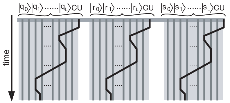
We need to ensure that we error correct all the qubits in our system. This means not only the computational qubits, but also the cus and the ‘buffer’ qubits – all those in a classical state that do not play an active role in the computation. To start with, we shall consider that all the classical states are stable, and just describe error correction for the computational qubits.
II.1 Coherent Correction Procedures
When error correction is performed, the scheme typically follows the process of performing syndrome extraction so that some ancilla qubits contain information on the errors. After that, the ancillas are measured and we act depending on the results in some fixed, logical way. Hence, we might as well include this logic in a quantum circuit that feeds the error information directly back to the encoded qubit. This way, the correction procedure is the same for every encoded qubit, independent of what errors have occurred. The information on what errors occurred is left in the ancilla qubits, which then need to be reset. This idea is illustrated in Fig. 5.
II.2 Ancilla Reset
In order to avoid needing to measure and correct, we need to be able to reset qubits that are in an unknown state to the state. To achieve this, we assume that our qubits are not just qubits but have a third level, which we can populate from either of the states and . However, we will also assume that this third level, which is at some higher energy than the computational states, has a dissipative decay to one particular state, say . This is essentially the same idea as algorithmic cooling Boykin et al. 2002. The reset procedure is denoted in our circuits by .
II.3 Switchable Parallelism

In order to perform computation on our device, we require the ability to switch between two different scenarios. Firstly, we need a cu for every encoded qubit, so that we can perform error correction on it. Secondly, we need a single cu in the computer so that we can perform the algorithmic part of our computation. Thankfully, we have already seen how we can switch a cu off – we just use the first steps of a two-qubit gate, where the control qubit is a classical state. This classical state indicates whether the cu should be left switched on or not. We can therefore consider a slight modification of our device structure. We have many repeating blocks of qubits, each encoding a single logical qubit. Adjacent to each block is another qubit, which is initialised in a classical state. All of these are set to , except for one, which is set to . This additional qubit in the block of is referred to as the Switching Station (ss).
Our computer starts off in error-correcting mode, i.e. with one cu for every logical qubit. When we want to perform a computational step, we move the cus to the sss (given the regular spacing of all the cus and sss, this happens simultaneously for all of them) and perform the first step of a two-qubit gate. This deactivates all the cus in a reversible manner in every ss, except for the one that is set to , leaving a single cu for performing the algorithmic steps that we require.
Ideally, between two phases of error correction we would be able to perform an arbitrary computational step. However, given the one-dimensional organisation of our computer, we have to accept that for increasing device size, this is impossible. Instead, when we have to perform gates between distant qubits, we substitute this for a series of swap gates to gradually move the qubits closer together, so that they can eventually be interacted. One subtlety, however, is that our single cu appears in a single position, and so we need an increasing number of steps just to move it into the correct position. In the same way that we can move a computational qubit along the array, we can move the cu’s starting position along the array. We achieve this by understanding how the deactivated cus are stored in a pattern of on physical qubits. Our single-qubit gate protocol allows us to create this pattern in the region where our cu remains switched on, and remove it from the next ss along.
II.4 Parallelism for Fault Tolerance

Benjamin originally introduced the idea of sss in Benjamin 2000, where he referred to them as sub-computers. Each sub-computer had a unique label, and the cus would perform a computation on each label to decide whether they should be deactivated, allowing arbitrary patterns of cus to be created. The concept of sss is much more limited – we only need two different patterns of cus. As a result, these sss only require a fixed proportion of the device size, whereas the labels for the sub-computers grew with . While this is still a relatively modest cost, the computation time to create arbitrary patterns of cus must require steps.
The next logical question is whether there are fixed patterns of cus that we can usefully create, while still requiring only a fixed proportion of the device size, and only requiring a fixed amount of the computation time. In particular, we would like to consider the configurations for fault-tolerance (FT). In this scenario, we desire the ability to switch from a single cu to sets of cus that are active every encoded qubits, where is an integer from 0 (the original ec pattern) up to some maximum level, . This is because an encoded qubit consists of computational qubits. Hence, when we concatenate a single level of code, the encoded qubits that we now produce consist of of the originally encoded qubits. This continues up the levels of concatenation, yielding the indicated power law. The number of levels of concatenation, , is independent of the number of qubits that we want to perform computation on, it only depends of the accuracy to which we desire our final computation. Hence, within our ss we could envisage qubits, each indicating whether a particular cu should be turned on at each level of concatenation. This would require a minimum of computation at each step (one gate), and still only requires a fixed proportion of the device size.
This expanded ss is actually more powerful than we require, and could be useful for some more advanced ideas, such as super-cus. The rationale behind a super-cu is that when we operate on concatenated codes, most of the operations that we perform can be done so bitwise. Instead of using a single cu and repeating the same operation many times, it would be more sensible to have a super-cu, which consists of a dense block of cus, allowing us to perform these bitwise steps with a single command. However, for the most simple form of fault-tolerance, this expanded ss is more complex than we require. Instead of qubits, we can reduce it to qubits, and a small additional computation. The point here is that we can organise it so that when we require a cu every qubits instead of every qubits, we only have to switch off cus (there is no need to reactivate any). As a result, we just need the label of the ss to say at which level the corresponding cu gets switched off. Hence, we only have to encode the numbers to , which can be achieved in qubits. Of course, we also have to store the single extra number () that marks the location of the single cu which we retain for performing the algorithmic steps of the computation.
| Initial Step () | ||
|---|---|---|
| Intermediate Steps | ||
| Final Step () |
We must still show how the actual process of activation/deactivation of cus occurs. To achieve this, we will start with a cu active in every ss44 4 If we are just switching from one level of concatenation to another, it will generally more efficient to by-pass this step, and just use the already active cus., and perform a small (reversible) computation on the label of the ss. This computation will output a single bit onto an ancilla qubit, which can be used for the activation/deactivation procedure as before. We give the required computation in Tab. 1. The concept of the circuit is quite simple to understand. We wish to determine if . Starting with the most significant bit of each, if , then and there is no need to continue Similarly, if , there is no need to continue. We then move to the next most significant bit. We only compare bit if all the more significant bits of and are equal. This continues until termination of the sequence, either because the answer is determined, or because we have run out of bits (in which case we must also know the answer, but the terminating step is consequently slightly different).
We therefore see that it is possible to generate sufficient parallelism for fault-tolerance. In subsequent sections, we will ensure that we have taken into account all necessary considerations by deriving a fault-tolerant threshold for our scheme. However, before we do this, we must consider all the other qubits in the system, not just the computational qubits.
III Error Correction of the Control Units
We have now presented a scheme that appears to be able to perform arbitrarily accurate computation on the one-dimensional globally controlled array, even in the presence of (small) errors. However, this scheme has implicitly assumed the stability of all the classical states in the system - all the padding states, the labels in the sss and the cus. If any of these become corrupted, the whole computation can become corrupted. As a first step towards protecting these, we can simply state that our regular device structure guarantees the locations of these classical states in a periodic way. Hence, potentially, we could create global pulses that just address these. For example, the B qubits should always be classical states (unless we’re in the middle of performing a two-qubit gate). By applying regular measurement to these classical states, we get a Zeno effect which prohibits transition of a classical state into its complement. In the long-run, this is not sufficient for arbitrarily accurate computation, but may delay the requirement for more aggressive schemes of error correction.
Eventually, we require the ability to perform error correction on the cus. The first step in doing this is to acknowledge that these are classical states and, hence, we only have to protect them against bit-flips, and not phase-flips. As such, we can use a classical repetition code to protect the information. We still intend to perform our computation with single cus, but at the error correcting stage we will switch on different sets of triples of cus. These triples will compare themselves to each other and attempt correction. This step is somewhat non-trivial because we must allow the potentially faulty cus to control their own actions, and yet we still need to be sure that the correction will result. One way in which this can be achieved was first presented in Kay 2005.
So, instead of using a single cu for a computation, we shall now use three of them. We do not intend to perform any part of the algorithm with all three cus present, as this will be less efficient than switching off two of them. We can initially align these with computational qubits. The patterning needs to be chosen with care in order to minimise the complexity of the protocol. We target an operation on a single qubit by applying a controlled-phase gate () with each of the three cus, separated by the single qubit rotations , , and applied to all the qubits. The resulting evolution on the targeted qubit is
Any qubits that are far enough away from the cus will not be affected by the s, and hence will be subject to the evolution , which we select to be the identity transformation i.e. . We need to create sequences such that we can apply an arbitrary rotation to the qubit we want, but do nothing to any of the other qubits. This necessarily includes qubits that get affected by one or two of the s. The first step is to select a patterning of the cus such that no qubit ever experiences 2 s (unless an error has occurred). The simplest example is to align the cus with qubits , and (note the gap, ).
In the fault-tolerant scenario that we have been describing, the most efficient way of introducing these three cus is by relabelling the switching stations using the following protocol. If the label was non-zero, add 1 to the value (these correspond to the qubits for each block). Label the zero-valued sss that are 1 and 3 sss away from these relabelled sss with the number 1 (corresponding to qubits and ). So, by deactivating all cus in regions controlled by sss with 0 labels, we get the regular patterning that is required, and we can still access the parallelism required for fault-tolerance. In fact, by repeating this procedure at every level of concatenation, this enables patterns of cus for fault-tolerance at a cost of a single extra bit in each ss.
The 1-2-4 arrangement of cus can still cause unavoidable applications of single gates,
Clearly, if we apply the sequence twice, all of these will be removed, while the targeted qubit experiences the evolution
which, given that we have a free choice of , and , must contain sufficient freedom to create any single-qubit rotation that we desire (up to a global phase).
Now that we are using a cu that has some redundancy in it, there is enough information to be able to correct for errors. There are two stages involved in making use of this information. Firstly, we must perform a syndrome extraction, placing information about any errors that have occurred on an ancilla qubit (which would otherwise have been a computational qubit). Secondly, we must feed back from this ancilla to be able to correct the faulty part of the cu.
If one of the cus suffers a bit flip, then only the targeted qubit will be affected. We can therefore neglect all other qubits, and just concentrate on the ancilla that we will be targeting, and which will initially be in the state . For the three bits that can get flipped, the resulting evolution will be one of
| or |
Using either or , the evolution when the cu has no error is 11. The results if there have been errors are shown in Table 2, where
is either 2 or 3, where . We thus have free choice of and to make this remaining evolution (for example, and ), which enables the error syndrome to be placed on the ancilla. Similarly, we can create the evolution just by changing to . If we wanted to create the Hadamard gate, we would set
| Error occurs on cu: | ||
|---|---|---|
| none | 11 | 11 |
| 1 | 11 | |
| 2 | ||
| 3 | 11 |

How can this information be used to correct the right error? If we apply , i.e. we have set , then the target (ancilla) qubit is flipped if there is an error on either of the first two cus. We then use the circuit in Fig. 8 to feed back the error syndrome from the ancilla to the first cu, where part (a) is controlled by both cus 2 and 3. If the error occurred on the second cu, then the feedback process won’t occur. Therefore, we can correct for a single error on any of the cus by repeating the process.
Alternatively, we could target the same ancilla with pulse sequences such as , which would flip the ancilla only if an error has occurred on the second cu. In the previous method, we created the local pattern of 2 s on neighbouring A qubits which is required to feed information back to the cus by using the cus. This is susceptible to error if a nearby B qubit that should be a gets flipped to a (the local pattern can be created in several places). However, this alternative technique allows us to make one of those s a fixed classical state (within the ss, say), and then we need concentrate on only flipping the one ancilla next to it. In this case, if only a single error occurs somewhere, correction is localised in the right area of the device, and is stable against other B qubits being flipped.
III.1 Stability of the Classical States
Now that we know how to keep the cus stable, it is relatively easy to see how to keep the other classical states stable. We don’t even need error correction, we just need to reset the qubits conditional on the presence of the now perfect cu. If the reset procedure is imperfect, then it just gets corrected in the next round of resets. This involves two steps, one which corrects those on qubits and another that corrects those on qubits. Both of these will occur in the regime where there is one cu activated for every ss. Resetting the buffers is simple - we just move the cu next to each of them and send out the reset command, much as we would for a single-qubit gate. This requires a fixed number of steps, independent of device size.
To correct the buffers, we move the cu adjacent to the result qubit in the ss (the one which is used as the control bit), and switch it to the state. We also do that to an adjacent qubit (i.e. the nearest physical qubit, not the next computational qubit). This creates the unique local patterning which is used to feed operations back onto the qubits (see Fig. 2). Hence we move all the buffer qubits between these two s and reset them. One potential risk is an interaction with the cu when it is adjacent to one of the s during the feedback process. Since the mechanism for the reset procedure will depend on the physical implementation, this question is difficult to answer, but we can at least say that if we were applying a unitary operation, there is no additional interaction.
One might think that the unique patterning, the same as found in the two-qubit gate, could be used to deactivate the cu, meaning that all the qubits should be in the state, so we could globally apply the reset procedure to all of them. Unfortunately, this process would also move the imperfections of the qubits onto the qubits, and, in turn, move some of the computational qubits onto qubits (if there are errors on some of the buffers). This reminds us that if there are imperfections in the qubits, these will be mapped onto the qubits, including the computational qubits. However, error correction will correct for these provided they occur sufficiently infrequently.
Having reset the buffer qubits, we need to reset, or otherwise stabilise, the qubits in the sss. We can use the different levels of concatenation in the fault-tolerant scenario to our advantage for performing resets of different organisations of qubits. Consider the scenario where we have a cu enabled for every sss. Between their own sss, there are sss which all store the value 0 and have deactivated cus. Thus, we can reset all of these. Note, however, that they can’t reset their own states. At higher levels of concatenation, there is a cu for every sss. Regularly spaced between each of these are sss which contain the number and deactivated cus that have not been corrected yet. So, we can move the active cus along and reset all of these. Eventually, at the top level of concatenation, there are some switching stations that have never been reset. We cannot correct them with the single cu (errors would build up too quickly as the device size scales), so this would appear to be a problem. However, it is not. We have gone to a level of concatenation that is as good as we need i.e. it is sufficiently good that it is safe to assume that the top level of concatenation is stable. Hence, it is acceptable for these cus to correct their own sss – the effect that we are concerned with is precisely the same effect as the termination of the hierarchy of concatenation instead of continuing it ad infinitum.
IV Error Correction of Quantum Cellular Automata
As we have presented it here, our physical model corresponds in a natural way to a particular realisation of quantum computation – optical lattices. In particular, we have assumed we can perform operations on the A qubits, controlled by the B qubits to their right (for example). Another global control scenario which, again, has a physical counterpart, is that our qubits can only determine the total spin of their neighbours, Benjamin 2001; Benjamin 2002; Benjamin and Bose 2003. Our global pulses then take the form of , which causes all the qubits to flip their value if the total spin of their neighbours is 0 (i.e. one qubit is spin up, and the other is spin down). This is precisely the model of quantum cellular automata (see Perez-Delgado and Cheung 2005 and references therein). All of the above work on error correction, cus, sss etc. can be developed in this scenario. However, there is one vital difference, in that all schemes that have so far been discovered require an encoding of the computational qubits across several physical qubits. This introduces an additional complication, which was carefully circumvented by our choice of physical model – the computational basis itself must be stabilised. In particular, the logical qubits exist inside a subspace of these physical qubits, and if a faulty pulse sequence causes a departure from this subspace, an error correcting code can do nothing about this. Some measures can be taken, such as stabilisation of the basis via the Zeno effect. This can potentially work to a similar level as error correction, in that we may be able to correct for a single error occurring between two Zeno pulses. However, it is still possible that two errors could occur, and ruin the computation. Hence, these ideas are not sufficient for a fully fault-tolerant scenario. Even after the work of the next section, therefore, the possibility of fault-tolerance in a quantum cellular automata remains an interesting open question. It may be solvable using the techniques of Lidar et al. 1999; Bacon et al. 2000; Wu et al. 2002; Byrd et al. 2005, where it is shown that it is possible to keep encoded qubits within a particular subspace, and especially Mohseni and Lidar 2005 where this is done under a form of global control. We have not, as yet, explored this possibility.
We can even justify that, using the concept of a cu, we must use an encoded basis for the CA model. This argument is simply a symmetry argument. Let us assume that we can encode the qubits and the cu in single spins. Since all the qubits will behave the same, and the cu must do something different to the computational qubits, we can envisage placing the computational qubits on s, and the cu on a . We then need to move the cu relative to the computational qubits.
If we were to send a pulse , then clearly we cannot do anything on just the cu. If we send a pulse , then we can perform operations on the neighbours of the cu by setting . However, by symmetry, both neighbouring qubits perform the same operations i.e. if we can find a sequence of pulses to propagate the cu to the left, it also moves to the right. We can either choose to use this symmetry in our system, which requires us to double its size, so the cu is encoded on 2 spins, or we can break the symmetry with respect to and by choosing an encoding of the computational basis over an even number of spins. Raussendorf and others have showed another way to use the symmetry of the system without requiring a cu in the system (effectively by using edge effects to replace the cu) Raussendorf 2005; Fitzsimons and Twamley 2006.
V Deriving Fault-Tolerance and Constructing the Circuits
Having presented a globally controlled architecture that supports fault-tolerance, we would now like to calculate the error rate below which the error improves with each round of concatenation, and hence below which we can make our computation arbitrarily accurate. The approach that we take is to follow the proofs of Aliferis et al. 2006, which provide a rigorous derivation of a threshold. The authors then proceed to evaluate this threshold under the assumptions of arbitrary parallelism, non-nearest neighbour interactions and the ability to perform measurements. Under the assumption of global control, we have to remove all these simplifications, so we expect the threshold to be significantly worse. As with initial threshold estimates, however, the important point is not how large or small such an error rate is, but that a critical error rate does exist. The ability to derive a threshold in this model is also very useful because it is closely related to quantum cellular automata Perez-Delgado and Cheung 2005, and whether fault-tolerant computation can be achieved with them. However, as previously described, there are still outstanding issues related to the fault-tolerance of a quantum cellular automaton.
The calculation of a fault-tolerant threshold proceeds approximately as follows. First of all, we select a universal (generally over-complete) set of gates that we want to work with. Then we construct our error correcting circuit out of these gates, ensuring that (in this case) a single error occurring within the circuit propagates to no more than one output qubit. We then take each gate in our universal set (constructed to act on an encoded qubit), and apply the error correction circuit to all the logical input and output qubits. This idea is shown schematically in Fig. 9 for the controlled-not gate acting on the Steane [[7,1,3]] code, where the controlled-not is implemented by applying it bitwise on the physical qubits.
The construction of our circuits has to take into account all the mechanisms that we require, such as the cus, the buffer qubits, nearest-neighbour interactions etc. One of the primary simplifying assumptions that we will make is that the cus and buffer qubits are stable. We can do this because we will be able to construct a fault-tolerant scheme for these, with their own threshold . We expect this threshold will be much larger than the threshold for the computation that we wish to implement (primarily because all the states are classical, so we just have to use a repetition code, which is vastly simpler). Since this threshold is much larger, we can assume that the time required to implement it is a negligible fraction of the computation time, and hence we can just neglect it.
In order to take into account the physical structure of our device, we shall formulate all the gates in terms of nearest-neighbour interactions, with the additional caveat that gate must be applied to a qubit that either is, or is adjacent to, the qubit that gate was applied to. In this way, we don’t have to worry about the cu running up and down the whole time, it just moves to its neighbour, costing a maximum of 3 swap operations. As such, the swap gates that we will add to the circuits are only present to correctly evaluate the number of ‘wait’ operations – we do not actually implement the swap operations. As such, the propagation of errors through these gates is irrelevant. In fact, this is very important because otherwise these swap gates could cause the errors to propagate to every qubit involved, which is certainly undesirable.
We also have to remember that we can only apply one gate at a time in each error correcting block, and that we have to apply the ‘do nothing’ operation on the rest of the qubits. This adds significantly to the number of steps in the scheme.
Now that we have written out the circuits under these constraints, we count up the number of locations in which an error can occur in each of the circuits. We then take just the gate (plus the error corrections) that has the largest location count (), as this will be the one the determines the threshold. Typically, this gate will be the one with the most inputs and outputs. If errors occur with probability independently at each location, then the probability of errors occurring within the circuit is
The motivation for the construction demonstrated in Fig. 9 now becomes clear – it was proven in Aliferis et al. 2006 that all single errors get corrected by these circuits. The probability of an error on the logical qubits is thus the probability that the error does not get corrected,
The approximation is valid because we expect (as will be confirmed in Sec. VIII) that is a small quantity. The computation can be performed to arbitrary accuracy provided , so equality gives an error correcting threshold, . The threshold can then be improved by enumerating the number of benign locations. These are the pairs of locations at which errors can occur and the logical qubits are still corrected. The first term in the expansion is therefore reduce from to .
| (1) | |||||
We intend to calculate the threshold for one particular error correcting code, the Steane 7-qubit code. Primarily, this is because the majority of gates can be performed on encoded qubits in a bit-wise manner, making them very simple. Secondly, this will give us a useful point of comparison with Aliferis et al. 2006, which also uses this code.
The aim of the remainder of this section is to describe general tactics that allow us to take a specific gate which acts on an encoded qubit and show how it can be performed, ensuring that if only a single error occurs in the circuit, only a single physical qubit from each encoded qubit is affected on the output (of course, we don’t mind what happens to ancillas, provided these errors do not propagate to the encoded qubit).
Naturally, some of our gate constructions are automatically fault-tolerant. In particular, any bitwise gates are fault-tolerant because there are no operations that can transfer an error from one physical qubit to another in the same encoded qubit. This highlights the reason for choosing the Steane code – a universal set of gates exists where only a single gate cannot be applied in a bitwise manner. Note that the gate , which we introduce in the next section allows other gates to be applied in a bitwise manner.
V.1 Propagation of Errors
In order to ensure that our gate constructions are fault-tolerant, it is important to understand how errors propagate between qubits. The following identities may be useful:
These essentially state that bit-flip errors propagate from control to target, whereas phase-flip errors propagate in the opposite direction. Hence, if we’re going to use some ancillas in the gate constructions, we will only have to ensure they’re correct with respect to one type of error, a more realistic task than protecting them against all errors.
V.2 Cat States and Majority Voting
The significant problem for fault-tolerant circuits arises when we have to output multiple operations onto a single ancilla, which is then used to feedback information onto the original qubits. See, for example, Fig. 5. In this example, syndrome extraction is achieved by performing four controlled-not gates, each controlled by the same ancilla (initially in the state), targeting the four different qubits from which we are extracting the syndrome. If an error occurs on this ancilla after the first controlled-not, for example, then it can feed through the other gates to affect the other three qubits.
This problem is circumvented by replacing the single ancilla with four ancillas, prepared in a ‘cat’ state, (named for Schrödinger’s cat). Each of the four controlled-nots is then controlled by a different ancilla. From there, we can take a vote between the four ancillas, onto a fifth, as to what the correct value is, and this can then be used as the control for the feedback operation. There are two different types of vote that we use, depending on the situation. We refer to these as weak and strong majority voting.
V.2.1 Weak Majority Voting
In the example discussed so far, we wanted to calculate the single bit which was the syndrome of a set of operators. We divided this into four separate operators, and the result that we required was the binary sum of these operators, since we only have to take into account the possibility that there is a single error anywhere. In fact, this is most easily achieved using a slightly modified version of the cat state,
| (30) |
This state is an equal superposition of all 4-bit strings with an even weight (i.e. an even number of 1s). If the four target qubits are in the correct -state, then this state is invariant. However, if one of them is faulty, one of the ancilla qubits is flipped and we have an equal superposition of all 4-bit strings with odd weight. Therefore, this difference is very easy to detect, each ancilla performs a controlled-not onto a fifth ancilla. If a single error occurs at this stage, then it is only this fifth ancilla which matters.
We now just have to be sure that the state in Eqn. (30) can be created fault-tolerantly from . Note that phase errors in the final state do not matter to us. We start by creating a cat state by applying to a single qubit, and then performing controlled-nots. If a bit-flip has occurred on the control qubit, then this propagates to all the target qubits. However, we will then apply a Hadamard to all the qubits, and hence convert these into phase-flip errors. These do not propagate to the computational qubits, only affecting the single ancilla bit at the end. If a phase-flip has occurred on one of the targets before the controlled-not, then the ancilla was in the state, and hence phase errors are irrelevant. Hence, if a single error occurs, it results in bit-flips on no more than one qubit in the state of Eqn. (30).
This operation is particularly apparent in the circuit for error correction, Fig. 15.
V.2.2 Strong Majority Voting
The other situation that we are interested in, although not explicitly given in Fig. 15, we refer to as strong majority voting. In this situation, we wish to detect the error on a particular qubit several times. For example, in Fig. 5, a particular computational qubit is targeted by three controlled-nots performing the syndrome extraction. If it were to suffer an error between these three, the error could propagate to a second qubit due to an incorrect determination of the syndrome. In this case, we want to provide a constant value for the syndrome extraction steps, stored on an ancilla. If the ancilla gets flipped at some stage, then the encoded qubit would be falsely corrected, but it would only introduce a single error, not two.
This proceeds by forming a cat state on several (say 4) ancillas, . Controlled-not gates are then applied, each controlled by a different ancilla and targeting the same qubit. These qubits can then be used to vote, onto a fourth ancilla, as to whether the qubit had suffered an error. If the state is more than a single flip away from the cat state, then it was caused by a fault on the computational qubit. An alternative methodology is depicted in Fig. 10.
VI Fault-Tolerant Gates
In order to calculate a threshold, we have to specify what set of gates we are going use. All the circuits which we construct must be in terms of these primitives. The list specified here is certainly not minimal, but the more gates we have, the simpler the circuits that we can construct.
- 1.
Hadamard Gate,
- 2.
Bit-Flip,
- 3.
Phase-Flip, , and root,
- 4.
controlled-not
- 5.
swap
- 6.
gate,
- 7.
Toffoli gate (controlled-controlled-not)
With this set of gates, we have to construct circuits on the next level of encoded qubits to implement the entire set, and a circuit to implement error correction of the encoded qubits (this circuit is referred to as ec), such that if a single error occurs in any of the circuits, this affects no more than one of the qubits on each logical qubit.
The construction of some of these gates requires some additional sub-circuits including, in particular,
- 1.
Preparation of cat states on physical qubits, .
- 2.
Conversion of logical qubit to a classical repetition code, denoted . e.g.
- 3.
Preparation of
- 4.
State preparation, particularly , using an input state Boykin et al. 1999.
- 5.
The error correction circuit, ec.
VI.1 Bitwise Gates
The gates , , , , c-not and swap are all applied bitwise, and are, therefore, comparatively simple. Their value of is almost entirely determined by the product of the number of applications of ec and the number of locations in an ec. There are slight differences if we assume we have a super-cu such that all 7 gates can be applied simultaneously, or whether we have to apply them one at a time (in which case there are a number of ‘wait’ operations, which contribute to the number of locations). However these are counted, the values of will not be comparable to some of the other gates.
Let us demonstrate the required counting with an example of an encoded cnot gate. Consider Fig. 9 ignoring, for now, the blocks of error correction. No two cnot gates act on the same qubits, so in principle all seven of them can be performed simultaneously. Each cnot gate counts as a single location, so this gate has 7 locations. Since this gate does not require any measurements, the result is the same when we remove the ability to perform measurements. If we remove the parallelism restriction, then only one gate can be applied at a time. Therefore, there are 13 locations for each of 7 time steps (12 locations where the ‘wait’ operation happens, and a single location for the cnot that we are applying). This gives 91 locations. With a restriction to gates between nearest-neighbours, we must introduce a series of swap gates to interlace the qubits from the two different logical qubits, as depicted in Fig. 11. The swap gates are not correctly ordered for the sake of space. However, it is clear that they can be implemented such that the cu would only have to jump to its nearest-neighbour to be able to implement the next gate. This requires a total of 42 swap gates, which are implemented one at a time. Hence, the total location count is . Finally, we move to the physical model, where we need to count the number of physical operations required to generate each of the interactions. In particular, to move the cu from one qubit to its neighbour requires 3 swap operations. Hence the total number of time steps increases by a factor of 4. The new location count is . However, this is actually somewhat misleading for a threshold argument because these additional swap gates only affect the lowest level of concatenation. All higher levels just act on logical qubits, which do not have these separations. We can take this into account when calculating the threshold. Let be the threshold for the first level of concatenation and higher, while is the threshold at the physical level. We can therefore write that
which should improve our threshold estimate, .
VI.2 The Gate
When constructing a universal gate set, one only needs either the Toffoli gate or the gate. The gate typically gives a lower threshold value due to the fact that it acts on fewer qubits. However, the Toffoli, as described below, is very useful to us because we perform so many of these gates during the coherent feedback part of error correction.
In order to apply the gate, we first make an ancilla state, , as detailed in Boykin et al. 1999. This is input to the circuit specified in Fig. 12, where the only additional component that we require is the gate , which is specified below.
VI.3 The Toffoli Gate
The Toffoli gate, or controlled-controlled-not, is the worst-case gate, simply because of the number of inputs and outputs. The typical fault-tolerant construction was first suggested by Shor Shor 1996, and has been altered to work deterministically in the absence of measurements Aharonov and Ben-Or 1999; Boykin et al. 1999. We might also consider an alternative construction, using Fig. 13. At first glance, this circuit would seem to be much worse because it includes 6 applications of , and hence 6 applications of , compared to only 2 applications in Boykin et al. 1999. However, we may be able to gain some advantage by surrounding each gate by ec circuits. In this case, all single errors are corrected within each gate. Hence the only pairs of locations which are not benign are contained within blocks of ec-gate-ec. Therefore, this could, potentially, represent a significant reduction in the number of non-benign pairs of locations, even if the number of locations has increased. Note that due to our available parallelism, we will also surround all the ‘wait’ operations with ecs as well.
We must remember that we are limited to nearest-neighbour interactions, which means that we must keep track of the locations of the ancilla qubits, and count the swap operations required to move past these as well. It may also be useful to note that it does not matter which qubit the target qubit is, the number of required operations is the same (a swap operation moves from the start of the circuit to the end).
It turns out that this operation is superior for a threshold under the most restrictive set of assumptions, which relates to our model of global control. Given that this represents an improvement, it is also relevant to ask whether it is more efficient to not include the Toffoli in our set of gates, and just expand it each time it is used in the ec circuit. This would allow us to use a gate with fewer inputs and outputs as the worst-case gate, which could, potentially counter-act the increase in size of the ec circuit.
VI.4 N
This is by far the most complicated gate, and follows the construction of Boykin et al. 1999. As specified in that paper, the action of the gate is to take two inputs. One is a logical qubit, , and the other is a set of 7 qubits, all in the physical state. The output is then of the form
However, we have chosen to represent this as a one-qubit gate to clearly indicate the fact that, in constructing this state, a single error can have a catastrophic effect on the logical states, and so they can no longer be used in the computation (only the physical qubits can).
The output of this gate is not a logical qubit, as with other gates. It is, instead, a classical repetition code. Given that we will never perform error correction on this circuit, this is perfectly allowable. Any gates that are controlled off this repetition code can be performed bitwise.
In essence, the gate is constructed by making use of the observation that the codewords of the Steane code have an even (odd) number of s for the () state. Hence, performing a weak majority vote from the codeword onto an ancilla gives one of the seven bits required for the classical repetition code. Since we must repeat this sequence seven times, controlled by the same qubits in the codeword, a strong majority vote should first be used. This would perhaps be the way that would give the smallest threshold (see Sec. VII.2), although we chose to directly follow the circuits given in Boykin et al. 1999, which replace the strong majority voting step with a stabilization process (syndrome extraction).
VII Fault-Tolerant Threshold for the Computation
VII.1 Circuit for ec
We have to be careful about the construction of a fault-tolerant error-correcting circuit. In particular, the error-correcting circuits previously shown, such as in Fig. 5 are not fault-tolerant, because if an error occurs on a qubit while the syndrome is being measured, the error remains on this qubit, and a different qubit is ‘corrected’. Instead, we need to create a different circuit, that protects against errors of this form by using a degree of redundancy, and then majority voting, as described in Sec. V.2.
In terms of the primitives defined, the circuit in Fig. 15 fulfills all the requirements of a circuit that corrects single errors on its inputs, and does not catastrophically propagate errors that occur during the circuit. Depending on how much parallelism is available (i.e. whether we can perform more than one operation simultaneously on a given block), the arrangement of ancillas (and in particular, the number of ancillas used) can be optimised to reduce the number of locations in the circuit.
Note that a single application of this circuit for error correction (while we require two applications for error correction) can also be used to fault-tolerantly prepare an encoded qubit in the state, just by supplying in place of the logical qubit to be corrected. Given that we only need to prepare the state at the beginning of any of our gates, we can incorporate this part in the application of the ec before the start of each gate, thereby reducing the required number of time steps.
For simplicity, we have left one important part out of the circuit in Fig. 15, which corrects a significant oversight in the circuit as shown. In particular, if a single error occurs on one of the computational qubits between sets of controlled-not gates that feed the error information onto the qubits, then not only do we have a fault on that qubit, but we apply a correction to a different qubit. This is avoided at the start of the circuit by performing a strong majority vote process on each of the computational qubits which is to be read more than once. In the following subsection, we will learn that we are further justified in not depicting this part of the circuit because the extra gates are benign with respect to the rest of the circuit, and hence makes a negligible difference to the threshold estimate that we will make (however, we must remember that this process takes a certain number of steps, and adds to the number of error locations on the rest of the circuit).
With this circuit in place, we are now in a position to enumerate the number of locations for each type of gate. These results are given in Tab. 3. We therefore take the Toffoli gate as being the one with the most locations (once we’ve placed error correcting units on each input and output). In this case , and an approximate error threshold is given by .
Gate Inputs No No Restricted NN Physical & Outputs restrictions measurements parallelism interactions Model , , , 1 7 7 49 49 196 cnot 2 7 7 91 637 2695 T 1 237 2023 4926 10498 34018 Toffoli 3 N/A 6279 41952 123663 447357 155 5 This output is a classical repetition code of 7 qubits, not an encoded qubit. N/A 1127 3078 5990 15692 ec N/A 142 1486 2928 4982 19724
VII.2 Benign Locations
In Aliferis et al. 2006, counting the benign locations for pairs of errors provided a significant enhancement to the fault-tolerant threshold. However, the task was far simpler in that paper because the gate constructions used far fewer operations (due to the availability of measurement, arbitrary parallelism and non-nearest-neighbour operations), and because the gates were constructed out of Clifford operators, which means that the effect of errors can easily be calculated by propagating the errors through the circuit, which can be efficiently simulated on a classical computer. As such, our task is far harder, and we do not intend to count all the benign pairs. However, we can make (or re-use from Aliferis et al. 2006) some very simple arguments.
- 1.
If there is a ‘wait’ operation, then the locations either side of it form a pair. If there are multiple wait operations in a row, then all possible pairs of locations are benign.
- 2.
This can be generalised because the circuits are constructed in such a way that if an error affects one qubit of the 7, then for all time it only affects this one, and its equivalent qubits in the other logical qubits of the gate. Hence, if a second error occurs on this qubit, it acts as only a single error, and, therefore, all pairs along these lines are benign.
- 3.
All pairs of locations in an ec that acts on the input qubits are benign Aliferis et al. 2006.
- 4.
Pairs of errors that occur on two different output ec blocks are benign. This is clear because there are no gates that can cause the two errors to be present on the same logical qubit.
- 5.
A single error that occurs within a strong majority vote (except for those on the output ancilla) is benign with respect to any single error that occurs externally to that process. This is because the majority vote clears the effect of that error, just leaving the single error which gets corrected. By using a cat state of at least 6 qubits, it can also be made benign with respect to pairs of errors that occur within the circuit.
VII.3 Threshold
We are now in a position to enumerate the number of operations required for each gate, and make a first estimate as to the number of benign pairs. We have chosen to split this into a series of steps, building up slowly to the final threshold. This allows us to see where the basic costs of a global control scheme come into effect. Firstly, we evaluate the threshold allowing arbitrary parallelism and measurements. For this, we get a value of . This is comparable to the value of , obtained by Aliferis et al. 2006, but indicates that our simple evaluation of the number of benign pairs actually misses a large fraction. This suggests that all further results would benefit from more rigorous accounting of the benign pairs.
If we disallow measurements, then not only do our gate sequences get larger, but we also have to include the Toffoli gate in our set of gates. As a result, the threshold sees its most significant hit at this point, where we find . If we further assume that we have only a single cu in each error correcting block, then all gates have to be performed sequentially, instead of in parallel, thereby adding a lot of extra ‘wait’ operations. These further reduce the threshold to . Next, we must add in sets of swap operations so that the gates are always performed between nearest-neighbours and, further, even single-qubit gates must be performed on adjacent qubits. These leave us with a threshold of . Recall that adding in these nearest-neighbour interactions would mean that the circuits are not fault-tolerant if we were to apply the swaps (although it is known how to make such a structure fault-tolerant Szkopek et al. 2006). However, in the present case, these gates just serve to count the number of operations while the cu is moving independently. Hence, this calculation is valid here, but not for a general nearest-neighbour scheme.
Finally, we must take into account the physical model where we actually have to perform 3 swap operations to move between adjacent computational qubits. As already discussed, however, this only has to be done at the lowest level of concatenation, which means that its contribution is not as significant as it might otherwise have been. The final threshold that we find is
This threshold simply provides a bound – the real threshold is certainly higher. However, the intention of this calculation was not to optimise this bound, simply to show that a bound exists for a global control scheme. In particular, theoretical calculations of thresholds, such as Aliferis et al. 2006; Aharonov and Ben-Or 1999, give results several orders of magnitude worse than current numerical computations indicate. For example, while Aliferis et al. 2006 calculates a threshold of , numerical estimates Knill 2004 put the threshold for similar assumptions to be closer to 0.03. We estimate that, had we used the strong majority voting version of the gate , instead of the version of Boykin et al. 1999, the threshold would have been approximately , although making an accurate count of the number of benign locations is more demanding.
VIII Fault-Tolerant Threshold for the Classical States
To finish the argument, we must now demonstrate fault-tolerant error correcting circuits for the classical states and calculate their threshold, . We expect such a threshold to be significantly larger because the encoding is much smaller (only 3 qubits as opposed to 7), and because our ecs only have to correct for one type of error – bit-flips. Phase-flips don’t affect the final result. Although only 3 cus may be active (per block), we have to remember that, actually, we are trying to stabilise all 7 of the cus associated with that level of concatenation.
As before, we must construct a list of the required operations, and build them out of the circuit primitives. In this case, the most costly operation will involve moving a cu’s resting place from one ss to its neighbour. At all levels of concatenation except the lowest, the move operation involves four controlled-not gates (two in each ss) and seven swap gates (to move the cu from one ss to the other). However, in our previous calculation of the threshold, we did not decompose the two-qubit gate into the one-qubit gate steps, we merely took it as a primitive. The cu’s manipulation of sss is exactly the same as a two-qubit gate, and so we shall count each of these as a primitive. At the lowest level of concatenation, we must also move past all the buffer qubits, requiring 28 swap operations instead.
Before and after this move operation, we must apply error correction to the cus. This involves changing the array of cus available (one step), and then performing the procedures described in Sec. III. These procedures correct one of the three cus, and hence must be repeated three times to ensure that errors do not propagate catastrophically. Subsequently, we use these 3 to reset all the cus from the previous level of concatenation. This step is necessary because we are not operating, in the end, on encoded qubits, but with the single cus and must therefore propagate the extra stability due to this round of error correction to all the cus. As a result, we have a total of locations at which errors can occur. This gives pairs of locations at which faults could occur. Making no effort to enumerate the benign pairs, we simply quote , realising that this is insignificant compared to the value of , above, as we expected. If we have a physical implementation in which we can match the main threshold, , and the classical states obey a threshold , then we can implement approximately
operations between each phase of error correction on the cus. Hence, the classical threshold will have an insignificant contribution to the overall threshold, justifying our exclusion of it from the full calculation. We have skipped over arguing that the operations we perform uphold the requirements of non-propagation of single errors. One could most simply justify that this can be done by moving to a 5-bit code instead of a 3-bit code. That way, even if a single error occurs during the error correction step, and discounting the particular bit being corrected, there are still 3 other unaffected bits forming a majority, and hence single errors can be prevented from propagating.
IX Summary and Conclusions
The main result of this paper is simply stated – that a globally controlled architecture has a fault-tolerant threshold which is a positive number. In achieving this result, we have made two basic assumptions. Firstly, we have treated the classical and quantum states as two distinct sections, and only errors on the computational qubits contribute to the final threshold. We have justified this by also calculating a threshold for the classical bits, which is much smaller. However, a more elegant approach would be to combine the two elements. The second, implicit, assumption is that our computer was correctly initialised with the required patterning of classical states. One might expect that our fault-tolerant protocols would enable us to correctly initialise these patterns from some smaller initial configuration but there is, as yet, no rigour behind these expectations.
Given that little effort was expended in optimising the threshold, one might expect that significant improvements can be made to the calculated value. One is also given hope, since it was observed in Kay et al. 2006 that moving to a global control scheme allows alterations to (in this case) typical optical lattice schemes, such as changing from red-detuned lasers to blue-detuned, which brings significant (order of magnitude) benefits to some decoherence mechanisms, thereby compensating for some of the cost of moving to such a scheme.
An open question that still remains is whether, for other global control schemes, the basis states (such as those required for use with cellular automata), can be stabilised. Our results only apply at the level of logical qubits, not the underlying physical model, except that the two coincide for our chosen model.
This work was supported by Clare College, Cambridge and the European Commission through the Integrated Projects SCALA (CT-015714) and QAP (IST-3-015848).
References
- Benjamin (2002) S. C. Benjamin, Phys. Rev. Lett. 88, 017904 (2002).
- Benjamin et al. (2003) S. C. Benjamin, A. Bririd, and A. Kay (2003), quant-ph/0308113.
- Kay (2005) A. Kay (2005), quant-ph/0504197.
- Kay (2006a) A. Kay, Ph.D. thesis, University of Cambridge (2006a), URL http://cam.qubit.org/users/Alastair/thesis.pdf.
- Christandl et al. (2004) M. Christandl, N. Datta, A. Ekert, and A. J. Landahl, Phys. Rev. Lett. 92, 187902 (2004).
- Christandl et al. (2005) M. Christandl, N. Datta, T. Dorlas, A. Ekert, A. Kay, and A. J. Landahl, Phys. Rev. A 71, 032312 (2005).
- Kay (2006b) A. Kay, Physical Review A 73, 032306 (2006b).
- Benjamin (2004) S. C. Benjamin, New J. Phys. 6, 61 (2004).
- Lloyd (1993) S. Lloyd, Science 261, 1569 (1993).
- Nielsen and Chuang (2000) M. A. Nielsen and I. L. Chuang, Quantum Computation and Quantum Information (Cambridge University Press, Cambridge, UK, 2000).
- Vollbrecht et al. (2004) K. Vollbrecht, E. Solano, and J. I. Cirac, Phys. Rev. Lett. 93, 220502 (2004).
- Kay and Pachos (2004) A. Kay and J. K. Pachos, New Journal of Physics 6, 126 (2004).
- Kay et al. (2006) A. Kay, J. K. Pachos, and C. S. Adams, Physical Review A 73, 022310 (2006).
- Calarco et al. (2004) T. Calarco, U. Dorner, P. Julienne, C. Williams, and P. Zoller, Phys. Rev. A 70, 012306 (2004).
- Aharonov and Ben-Or (1999) D. Aharonov and M. Ben-Or (1999), quant-ph/9906129.
- Boykin et al. (2002) P. O. Boykin, T. Mor, V. Roychowdhury, F. Vatan, and R. Vrijen, Proc. Natl. Acad. Sci. USA 99, 3388 (2002).
- Benjamin (2000) S. C. Benjamin, Phys. Rev. A 61, 020301 (2000).
- Benjamin (2001) S. Benjamin (2001), quant-ph/0104117.
- Benjamin and Bose (2003) S. C. Benjamin and S. Bose, Phys. Rev. Lett. 90, 247901 (2003).
- Perez-Delgado and Cheung (2005) C. A. Perez-Delgado and D. Cheung (2005), quant-ph/0508164.
- Lidar et al. (1999) D. A. Lidar, D. Bacon, and K. B. Whaley, Phys. Rev. Lett. 82, 4556 (1999).
- Bacon et al. (2000) D. Bacon, J. Kempe, D. A. Lidar, and K. B. Whaley, Phys. Rev. Lett. 85, 1758 (2000).
- Wu et al. (2002) L.-A. Wu, M. S. Byrd, and D. A. Lidar, Phys. Rev. Lett. 89, 127901 (2002).
- Byrd et al. (2005) M. S. Byrd, D. A. Lidar, L.-A. Wu, and P. Zanardi, Phys. Rev. A 71, 052301 (2005).
- Mohseni and Lidar (2005) M. Mohseni and D. A. Lidar, Phys. Rev. Lett. 94, 040507 (2005).
- Raussendorf (2005) R. Raussendorf, Phys. Rev. A 72, 052301 (2005).
- Fitzsimons and Twamley (2006) J. Fitzsimons and J. Twamley, Phys. Rev. Lett. 97, 090502 (2006).
- Aliferis et al. (2006) P. Aliferis, D. Gottesman, and J. Preskill, Quant. Inf. Comput. 6, 97 (2006).
- Boykin et al. (1999) P. O. Boykin, T. Mor, V. Roychowdhury, and F. Vatan (1999), quant-ph/9907067.
- Shor (1996) P. W. Shor, in 37th Annual Symposium on Foundations of Computer Science (IEEE Press, 1996), pp. 56–65.
- Szkopek et al. (2006) T. Szkopek, P. Boykin, H. Fan, V. Roychowdhury, E. Yablonovitch, G. Simms, M. Gyure, and B. Fong, IEEE Trans. Nano. 5, 42 (2006).
- Knill (2004) E. Knill, Quantum computing with very noisy devices (2004), quant-ph/0410199.