Non-universal level statistics in a chaotic quantum spin chain
Abstract
We study the level statistics of an interacting multi-qubit system, namely the kicked Ising spin chain, in the regime of quantum chaos. Long range quasi-energy level statistics show effects analogous to the ones observed in semi-classical systems due to the presence of classical periodic orbits, while short range level statistics display perfect statistical agreement with random matrix theory. Even though our system possesses no classical limit, our result suggest existence of an important non-universal system specific behavior at short time scale, which clearly goes beyond finite size effects in random matrix theory.
Keywords:
many body system, quantum dynamics, quantum chaos, classical chaos, quantum statistics,periodic orbitspacs
05.30.-d,05.45.Mt,05.45.PqI Introduction
One of the key discoveries of quantum chaos has been the so-called quantum chaos conjecture, originally proposed in Refs. qcc a. It claims that even simple non-integrable quantum systems, whose dynamics is sufficiently complex (say, dynamically mixing in the classical limit), possess quantum fluctuations which can be described by a universal ensemble of random matrices without any free parameters Mehta 1991. Although a strict mathematical proof of this conjecture is still missing, its theoretical understanding has recently been considerably deepened qcc b. Still, it is known from the early years of quantum chaos Berry 1985, that level fluctuations exhibit universal features only on sufficiently small energy scales, or long time scales, whereas one obtains system specific non-universal features on long energy scales (short time-scales) which can be usually understood and computed in terms of classical orbits.
Therefore it seems that the picture is quite complete and satisfactory for systems possessing a well defined classical limit. But what about simple systems which do not have a classical limit, e.g., systems of interacting fermions, or systems of interacting qubits? In such systems, dynamical complexity can be reached in the thermodynamic limit of many interacting particles Prosen 1999a. In some exactly solvable cases formal similarities between the thermodynamic limit and the semi-classical limit can be established Prosen 1999b. For example, one may start by considering simple, non-integrable, many-particle Hamiltonians with local interaction which are specified by only a few (non-random) parameters. Can quantum spectral fluctuations of such systems be described by universal ensembles of random matrices? If yes, what are the energy scales of such universality? Is there a breaking of universality at sufficiently large energy ranges? How does the universality breaking scale in the thermodynamic limit? In this paper we address these questions in a simple dynamical system, namely an Ising chain of spin particles on a 1d ring, kicked periodically with a homogeneous, tilted magnetic field. We performed careful numerical calculations of quasi-energy spectra and their statistical analysis. For appropriate values of model’s parameters, corresponding to strong integrability breaking, we indeed find both, the universality regime for sufficiently small energy scales, where no statistically significant deviations from random matrix prediction of infinitely dimensional Circular Orthogonal Ensemble (COE) could be detected, and a non-universality regime for large energy scales (or small times, corresponding to few kicks), where clear, statistically significant deviations from Random Matrix Theory (RMT) prediction have been found. Most notably, our analysis shows that the spectral form factor exhibits significant deviations from RMT at the time scale corresponding to one or few kicks (Floquet periods). This result could be intuitively understood as a qubit analogy of “shortest periodic orbit” correction, but its precise theoretical understanding is at present open.
II The system
The system we study is a kicked Ising chain (KIC) Prosen 2002, namely a ring of spin particles which interact with their nearest neighbors via a homogeneous Ising interaction of dimensionless strength and being periodically kicked with a homogeneous magnetic field of dimensionless strength . During the free evolution, i.e. between the kicks, the system evolves with the unitary propagator
| (1) |
and the action of the kick is described by the unitary operator
| (2) |
with being the Pauli matrices of particle and . The Floquet operator for one period is thus
| (3) |
We must also impose periodic conditions in order to close the ring: . During this paper we shall use the so called computational basis, which is composed of joint eigenstates of . This set of basis states can be written as .
In order to understand the spectrum one must first discuss the symmetries in the system. Let us start with the translational symmetry. The corresponding operator is defined on the computational basis as , and is extended to the entire Hilbert space by linearity. The action of this operator is to rotate the particles in the ring by one site. The eigenvalues of are with . Hence the Hilbert space is foliated into subspaces . The evaluation of the dimensionality of each of these subspaces is described in Appendix A. The evolution operator (3) is translationally invariant, and hence .
The next symmetry is an external reflection . Its action on the basis reads , and also . The two symmetries, and , do not commute. It must be noticed that if , then . This provides an additional symmetry within the subspace (and for even ). Thus these marginal subspaces are regarded as “special” and have slightly different properties than the rest. We shall not consider them for the purpose of statistical analysis in this article.
Finally, we define the anti-unitary symmetry . It acts as a mirror reflection within each spin with respect to the plane that contains both and the unitary vector in the direction (the direction of the Ising interaction). We can rotate our coordinate system around the axis in each qubit so that only has components in the and directions. Then, is simply complex conjugation, provided that and are set real, as is the usual choice. This symmetry operation also changes the sign of the momentum. Composing , we arrive to an anti-unitary symmetry that preserves the momentum i.e. an anti-unitary symmetry within each .
Concluding, has a rotational symmetry that foliates the spectrum into different sectors; the sector has identical spectrum as the sector . Hence for a fixed number of qubits we expect to have a maximum of relevant sectors, each sector having a Hilbert space dimension . Since each sector has an internal anti-unitary symmetry, we shall compare the statistical properties of system’s spectrum to those of Dyson’s Circular Orthogonal Ensemble Mehta 1991 of random matrices, of appropriate dimension.

For the rest of the presentation we fix parameter values of our system , for which the integrability of the model is strongly broken. We believe that for these parameter values the system is a generic representative of quantum chaos. Using highly optimized numerical methods (see appendix B) we have been able to diagonalize the model accurately for sizes up to qubits. The eigenvalues of the Floquet propagator have been written as , where are known as quasi-energies, and have been grouped with respect to the known quasi-momentum . Statistical analyses of desymmetrized quasi-energy spectra and their interpretation are given in the following sections. In order to compare with the RMT formulae we normalize the quasi-energies, i.e. write , in order to have mean level spacing equal to one ( denotes the dimension of the Hilbert space). Similarly, will denote the spectral variable, unfolded to a unit mean level spacing.
III Universality regime

Let us first analyze the most commonly studied spectral statistics of chaotic systems, that is the nearest neighbor level spacing distribution . is the probability that the distance between two nearby (unfolded) quasi-energies is between and . has been computed for the KIC and compared to the exact random matrix COE result (computed from Pade approximants Dietz and Haake 1990) with satisfactory results (not shown). However, since the details of such plot depend on the size of the binning of histograms, we prefer to show the cumulative (integrated) level spacing distribution . In fig. 1 we show a comparison of , both for the KIC and the exact infinitely-dimensional COE result, with the Wigner surmise . The expected statistical fluctuation of cumulative probability can be estimated Prosen and Robnik 1993 as
| (4) |
and gives a very realistic estimate of actual fluctuations of our dynamical system. We plot the results both for individual quasi-momentum subspaces, and averaged over all . In conclusion, based on the nearest neighbor level spacing distribution we find no significant deviations from universality, i.e. from COE model statistics.

Further on, we have studied other statistical measures of quasi-energy spectra, which are more sensitive to long-range spectral correlations, namely the number variance and the form factor Mehta 1991. The spectral form factor , is defined for discrete time as , and for infinitely dimensional COE has the form
| (5) |
denotes the discrete Heisenberg time, namely the number of kicks in which the average quasi-energy level separation grows to . Asymptotic finite dimension corrections to the form factor have been computed, and for small , the result reads
| (6) |
The number variance gives the variance of the number of levels in an unfolded spectral interval of length . The RMT formula for infinitely dimensional COE predicts a monotonically increasing variance , where is the Euler constant Mehta 1991. However, for a finite spectrum of quasi-energy levels this is not possible, since when the energy difference reaches the range of the spectrum the number of levels counted will always be the maximum and hence the number variance will be zero. For arbitrary finite dimension , there is an exact relationship Prosen et al. 2001 between and that accounts for the finite range of the spectrum:
| (7) |
Truncating the above series at finite with the form factor given by eq. (6) provides an excellent asymptotic approximation to the COE number variance for finite .

In figure 2 we compare the spectral form factor of the KIC with the infinitely dimensional COE, on a global time scale (on the order of Heisenberg time ). Of course, since the form factor is not self-averaging we had to perform some averaging over short time-windows in order to wash away the statistical fluctuations. We find no notable deviation from the COE. In order to estimate the expected fluctuations due to a finite sample of systems (namely a set of quasi-momenta ) we have also generated a similar average over the same number of random matrices of equivalent size. In the inset we plot the deviations of the form factor computed for the KIC, and the corresponding finite average over random members of the COE, from the exact RMT prediction. We observe that both behave similarly. In addition, we find very good agreement for the number variance of the KIC with the infinitely dimensional COE on short and intermediate spectral ranges (see fig. 3). In the inset the finite size fluctuations are also compared with the ones computed from appropriate finite samples of finite dimensional COE. Again we observe agreement.
IV Deviations from universality

As explained in the previous section, we expect that the number variance for a finite spectrum reaches a maximal value at (i.e. ). Actually as already mentioned, one can compute a good analytical approximation to COE averages of number variance for finite using eq. (7), and the saturation can be understood as a consequence of discreteness of time in the sine-like transformation on the RHS of (7).
Do the spectra of KIC in the regime of quantum chaos follow the same saturation as would be expected for typical members of the COE or not? We have performed detailed numerical checks of these questions and report the results in the following figures. In fig. 4 we plot the number variance for two different number of qubits (14 and 18), for the KIC. We find a very clear and notable difference: the data for the KIC tends to saturate at different, lower value of the unfolded spectral parameter , than COE, which typically saturate only at . Furthermore, the plateau is quite notorious. In the next plot (fig. 5) we have determined the saturation threshold and the saturation value as a function of the number of qubits .
Numerical results suggest that , namely that is proportional to though it is smaller by a large constant factor. The saturation value thus increases logarithmically with , or linearly with .

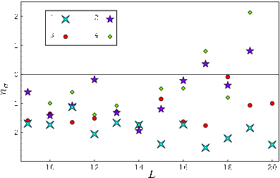
Perhaps a more clear picture is obtained after going into the time domain and inspecting the form factor for a few kicks, which correspond to large spectral ranges of . This regime is analogous to the non-universality regime corresponding to the shortest classical periodic orbit in quantum chaotic systems with well defined (semi)classical limit. However, we should not forget that our spin chain does not have any well defined classical limit or semi-classical regime. Still, it seems that , , etc., notably deviate from expectations of COE of the same dimensions as the KIC propagator. Indeed, in fig.6 we show as a function of , both for individual quasi-momentum subspaces and the average over all relevant , and find very clear and systematic deviation from COE expectation . Furthermore, deviation of is much bigger that expected COE fluctuation of which can be computed as Actually, in the limit , few higher moments can be computed as well and COE distribution of is conjectured to be exponential. In fig. 7 we plot the relative deviation of , for , from expected COE average in terms of the number of expected standard deviations. It is clear that, at least for one kick, the deviation is exceeding COE model significantly. Namely we find the deviation in the same direction for all different numbers of qubits , and for almost all it is exceeding two standard deviations. We also find statistically significant deviations from COE for other values of , in particular for , while the deviations for even arguments are less clear and conclusive.
A specialized reader may inquire for a comparison with the DODO random matrix ensemble (which resembles semi-separable systems Prosen et al. 2001). We note that the deviations from the COE observed in this article cannot be accounted by the semi-separable structure of the Floquet operator (3).
V Conclusions
We have performed numerical calculations of large quasi-energy spectra of an interacting multi-qubit system, namely the kicked Ising chain. No analytical solution of the model is known, i.e. the model is believed to be non-integrable. Consistently with previous results in the literature Pineda et al. 2006, we find good agreement of short-range level statistics of the model with Dyson’s ensemble of circular random matrices. However, when looking in detail at certain long-range spectral statistics, corresponding to short-times, we find notable and significant deviations from random matrix theory. This result reminds of non-universal regimes in semi-classical chaos widely studied in the 1990’s. However, this behaviour cannot be attributed to periodic-orbits, since the system lacks any sensible definition of a classical limit.
We believe that the numerical results are intriguing and await for theoretical explanation, perhaps in the direction of suggesting a new, abstract semi-classical picture (perhaps along the lines of Ref.K. S. Gibbons et al. 2006).
Acknowledgements.
We acknowledge discussion with T. H. Seligman and F. Leyvraz. We are grateful for many insights gained in discussions with C. Bunge and E. Brady. The work of C.P. was supported by Dirección General de Estudios de Posgrado (DGEP). T.P. acknowledges support from Slovenian Research Agency (program P1-0044 and Grant No. J1-7347). CP thanks the University of Ljubljana and its group for Nonlinear Dynamics and Quantum Chaos for hospitality.References
- qcc (a) G. Casati, F. Valz-Gris and I. Guarneri, Lett. Nuovo Cimento 28, 279 (1980); O. Bohigas, M.-J. Giannoni and C. Schmit, Phys. Rev. Lett. 52, 1 (1984).
- Mehta (1991) M. L. Mehta, Random Matrices (Academic Press, San Diego, California, 1991), 2nd ed.
- qcc (b) S. Müller, S. Heusler, P. Braun, F. Haake and A. Altland, Phys. Rev. Lett. 93, 014103 (2004); Phys. Rev. E 72, 046207 (2005).
- Berry (1985) M. V. Berry, Proc. R. Soc. London, Ser. A 400, 229 (1985).
- Prosen (1999a) T. Prosen, Phys. Rev. E 60, 3949 (1999a).
- Prosen (1999b) T. Prosen, Phys. Rev. E 60, 1658 (1999b).
- Prosen (2002) T. Prosen, Phys. Rev. E 65(3), 036208 (2002).
- Dietz and Haake (1990) B. Dietz and F. Haake, Z. Phys. B 80, 153 (1990).
- Prosen and Robnik (1993) T. Prosen and M. Robnik, J. Phys. A 26, 2371 (1993).
- Prosen et al. (2001) T. Prosen, T. H. Seligman, and H. A. Weidenmüller, Europhys. Lett. 55(1), 12 (2001).
- Pineda et al. (2006) C. Pineda, R. Schafer, T. Prosen, and T. Seligman, Phys. Rev. E 73(6), 066120 (2006).
- K. S. Gibbons et al. (2006) K. S. Gibbons, M. J. Hoffman, and W. K. Wootters, Phys. Rev. A 70, 062101 (2006).
- (13) F. Leyvraz, private communication, 2006.
- Ketzmerick et al. (1999) R. Ketzmerick, K. Kruse, and T. Geisel, Physica D 131, 247 (1999), eprint cond-mat/9712209.
- Berrondo et al. (1986) M. Berrondo, A. V. Bunge, and C. F. Bunge, Computers & Chemistry 10, 269 (1986).
Appendix A Dimensions of the invariant subspaces
Consider the computational basis of the Hilbert space of qudits . Let us generalize the translation operator allowing the ’s to have integer values between 0 and . The Hilbert space is foliated into subspaces such that for any , and . Let be the orthogonal projection operator, such that , for any . An elegant solution to the problem of calculating is presented here, following ley.
We first study the condition under which a state is projected to the null ket (zero vector). Let be the smallest positive integer such that ; we call the primitive period of . The action of the projection operator on is
| (8) |
with . Notice that if and only if . Since is the sum of a geometric series, its calculation is straightforward: if and only if . As a conclusion we obtain that if and only if .
Define the equivalence relation in as: if there exists an integer such that . Furthermore, if , then , but if , then . In other words, elements in different equivalence classes, are projected to orthogonal states. Thus counting the equivalence classes which are not projected to yields .
Let be the number of equivalence classes whose elements have given primitive period . If we call the number of elements in that have primitive period , then, . Notice that
| (9) |
as the only allowed values for are the divisors of . Using Möbius inversion formula we obtain
| (10) |
Möbius function is defined over the positive integers as , if is divisible by the square of a prime, and in any other case, where is the number of prime factors of . Then, collecting our results,
| (11) |
since the only possible primitive periods are the divisors of . However the value of is well approximated by for large values of .
Appendix B The optimal basis for diagonalization of KIC
To get the spectra used in this paper, it is crucial to develop an optimal diagonalization scheme. Though the techniques relaying on Lanczos method Ketzmerick et al. 1999 are fast they are not completely reliable. They loose precision as soon as some eigenvalues are close enough. In our experience the Lanczos method allows to obtain the full spectra for systems of up to 21 qubits, but the intrinsic numerical error becomes comparable to the mean level spacing. Even for 18 qubits, the biggest numerical error in one level is already bigger than the smallest inter-level spacing. As we are performing very precise tests we require that our levels are highly reliable, making Lanczos a prohibitively inexact method. We prefer using direct diagonalization with specialized routines Berrondo et al. 1986.
Let be the symmetrized version of , which however has the same spectrum due to unitary equivalence. Using an appropriate basis is important both to take advantage of the natural block diagonal decomposition of (due to symmetry ) and its symmetric character (due to symmetry ). The basis is constructed as follows. Let be a representative of a class defined by (see App. A), and such that . If then both are used as members of the basis. If at least one of is not the null ket, and can be incorporated into the base. By choosing from all different classes we build a complete basis in . Moreover, this basis is invariant under and is orthogonal.