Decoherence of two qubit systems:
A random matrix description
Abstract
We study decoherence of two non-interacting qubits. The environment and its interaction with the qubits are modelled by random matrices. Decoherence, measured in terms of purity, is calculated in linear response approximation. Monte Carlo simulations illustrate the validity of this approximation and of its extension by exponentiation. The results up to this point are also used to study one qubit decoherence. Purity decay of entangled and product states are qualitatively similar though for the latter case it is slower. Numerical studies for a Bell pair as initial state reveal a one to one correspondence between its decoherence and its internal entanglement decay. For strong and intermediate coupling to the environment this correspondence agrees with the one for Werner states. In the limit of a large environment the evolution induces a unital channel in the two qubits, providing a partial explanation for the relation above.
pacs
03.65.Yz,03.65.-w,03.65.Ud1 Introduction
In recent experiments [1, 2, 3, 4] it has been demonstrated that it is possible to protect ever larger entangled quantum systems, often arrays of qubits, ever more efficiently from decoherence. This improved protection of states makes a more detailed analysis of decoherence desirable. In the context of fidelity decay, a random matrix description [5, 6] is accessible and very effective in describing experiments [7, 8, 9]. A close connection between the dynamics of fidelity decay and decoherence has been shown in some instances [10, 11], which suggests to apply methods successful in one field to the other. Based on some previous work we shall therefore analyse in detail the consequences of using random matrix theory (RMT) to model decoherence [6, 12, 13] for the case of two non-interacting qubits or a single qubit as the central system.
Two perspectives make such a random matrix treatment particularly attractive. First, reduction of decoherence may, in some instances, be achieved by isolating some “far” environment (including spontaneous decay) to a degree that it can, to first approximation, be neglected. Then it can happen that the Heisenberg time of the relevant “near” environment is finite on the time scale of decoherence. In such a case it becomes relevant that RMT shows, in linear response approximation, a transition from linear to quadratic decay at times of the order of the Heisenberg time. This behaviour is seen with spin chain environments [14], and is essential for the success of the theory in describing the above mentioned experiments of fidelity decay. Note also that the concept of a two stage environment has been used for basic considerations [15]. Second, the long term goal must be to describe in one theory the decay of fidelity that includes undesirable deviations of the internal Hamiltonian of the central system, together with decoherence.
This study is focussed on weak coupling of one or two qubits to an environment, and thus we can use the correlation function approach proposed for purity decay in echo-dynamics [16], treating the coupling as the perturbation [6]. The linear response approximation will be sufficient and in this approximation the ensemble averages, which we have to take in any RMT model, are feasible though somewhat tedious. Exact solutions, which exist in some instances for the decay of the fidelity amplitude [17, 18], seem to be out of reach at present, because they would require the evaluation of four-point functions.
Assume that the qubit(s) are initially in a pure state, and evolve under their own local Hamiltonians. The qubit(s) are coupled independently via random matrices to a large environment in turn described by another random matrix. The coupling to the environment gives rise to decoherence. Averaging both the coupling and the environment Hamiltonian over the RMT ensembles yields the generic behaviour. We then focus on the correspondence between decoherence and entanglement decay for a Bell state. We find a relation between this two quantities, that can be partially understood assuming unitality. This relation in most cases coincides with the corresponding one obtained for Werner states. For that part, it is essential that the two qubits do not interact. Otherwise, the coupling between the qubits would act as an additional sink (or source) for internal entanglement – a complication we wish to avoid. However, a residual coupling between the qubits should be taken into account at some point [19]. A preliminary study of some aspects of this system has been presented in [13], but here we shall present a more general picture: First, we allow for local one-qubit Hamiltonians. They have a considerable effect on decoherence. Second, we cover exhaustively all possible initial states. Third, we study the consequences of the whole system being time-reversal invariant. Indeed, we present the mathematical procedure in detail using both the Gaussian unitary (GUE) and the Gaussian orthogonal (GOE) ensembles [20, 21] for the description of the environment and the coupling. The two ensembles correspond to time reversal invariance (TRI) breaking and conserving dynamics respectively. All these cases are treated on equal footing.
In section 2 we shall state the model, recall the linear response formalism for echo dynamics, and show how it can be adapted to forward evolution. In section 3 we shall discuss decoherence of a single qubit, which already shows some interesting features by itself and serves as a warm up for the more complicated case of two qubits. The details of the calculations are given in the appendices. This shall be treated in section 4, starting from the situation where one qubit is a spectator, exerting influence only through entanglement. More general cases are analysed and reduced to the spectator situation. Most analytic results will be accompanied by Monte Carlo simulations. In section 5 we investigate the correspondence between decoherence (purity) and entanglement (concurrence) as both evolve in time. We end with conclusions in section 6.
2 General considerations
In this section, we describe the general framework for our study of decoherence. We consider one- and two-qubit systems, coupled to an environment which is modelled using random matrix theory. The one-qubit case is introduced in section 2.1, the two-qubit case in section 2.2. The quantities studied in this paper are defined in section 2.3 and the tools used to solve the problem are introduced in section 2.4.
2.1 The model for one qubit
We describe decoherence by considering explicitly the additional degrees of freedom (henceforth called “environment”) which are interacting with the qubit. We follow the unitary time evolution of a pure, initially separable, state in the product space , where (of dimension two) and (of dimension ) denote the Hilbert spaces of the qubit and the environment, respectively. As time evolves, the qubit and the environment become more and more entangled, which means that after tracing out the environmental degrees of freedom, the state of the qubit becomes more and more mixed. For such a setup, the Hamiltonian is of the following form
| (1) |
Here, represents the Hamiltonian acting on the qubit, the Hamiltonian of the environment, and the coupling between the qubit and the environment. The real parameter controls the strength of the coupling. For notational ease, and if there is no danger of confusion, we omit extensions with the identity, as it is done in (1).
We describe both the coupling and the dynamics in the environment within random matrix theory. To this end, and are chosen from either the GUE or the GOE, depending on whether we wish to describe a TRI breaking or TRI conserving situation. The Hamiltonian implies another free parameter of the model, namely the level splitting of the two level system representing the qubit.
We shall study the time evolution of an initially pure and separable state
| (2) |
where and . At any time , the state of the whole system is thus , and the state of the single qubit is . While the state of the qubit is yet another free parameter in our model, we assume the state of the environment to be random. This means that the state is chosen from an ensemble which is invariant under unitary transformations. In practice, this means that the coefficients are chosen as complex random Gaussian variables, and subsequently the state is normalized.
2.2 The model for two qubits
For the two qubit case, we need to introduce the additional Hilbert spaces of dimension two and of dimension , which correspond to the second qubit and its environment respectively. As in the one-qubit case, the dynamics in the space of the two qubits (henceforth called “central system”) is obtained by considering the unitary evolution in whole Hilbert space and subsequently tracing-out the environmental degrees of freedom (henceforth called “environment”). As initial states, we use pure states in the whole Hilbert space, which are separable with respect to any combination of , , and :
| (3) |
Typically, we assume that at the two qubits (and hence the state ) to be entangled. This is the main new ingredient, as compared to the one-qubit case. In this work we shall consider three different dynamical scenarios, all explicitly excluding any interaction between the two qubits:

- (a)
The spectator Hamiltonian: In this case the two qubits evolve under separate Hamiltonians and acting on the Hilbert spaces and , respectively. In addition, we assume that only the first qubit is coupled to an environment, such that the total Hamiltonian reads
(4) where , , and are defined as in (1). This situation is shown schematically in figure 1(a). If we choose an initial state where the two qubits are already entangled, this provides the simplest situation which allows to study entanglement decay. If the two qubits are initially not entangled, the process reduces effectively to the one-qubit case, described previously section 2.1. The special case has been considered in Ref. [13].
- (b)
The separate environment Hamiltonian: This case differs from the spectator model only inasmuch as the second qubit is also coupled to an environment. Both environments are assumed to be non-interacting. The total Hamiltonian then reads
(5) where and describe the coupling to – and the dynamics in the additional environment. Both quantities are chosen independently from the respective random matrix ensembles, in perfect analogy with and . The real parameters and fix the coupling strengths to either environment. This model, see figure 1(b), may describe two qubits that are ready to perform a distant teleportation, where each of them is interacting only with its immediate surroundings. It can also represent a pair of qubits that, although close together, interact with different and independent degrees of freedom.
- (c)
The joint environment Hamiltonian: The third case, shown in figure 1(c), describes a situation in which both qubits are coupled to the same environment, even though the coupling matrices are still independent. In that case, the total Hamiltonian reads
(6) where describes the coupling of the second qubit to the environment. It is chosen independently from the same random matrix ensemble as .
2.3 The measures
As a measure of decoherence we use purity. This measures the degree of mixedness of a density matrix representing a physical system. Purity is defined as
| (7) |
It reaches a maximum value of one when the state is pure, i.e. when for some . Otherwise it is less than one and reaches a minimum when the state is completely mixed. We use purity instead of e.g. the von Neumann entropy because it is simpler to handle from an algebraic point of view. Note that for one qubit both quantities are equivalent, and for two qubits they contain similar information [22].
The other measure considered here is concurrence. It quantifies the degree of entanglement of two qubits in a pure or mixed state. It is a measure used extensively in the literature [23] that is straightforward to calculate. It is closely related to the entanglement of formation, which measures the minimum number of Bell pairs needed to create an ensemble of pure states representing the state to be studied [24]. Given a density matrix representing the state of two qubits, concurrence is defined as
| (8) |
where are the eigenvalues of the matrix in non-increasing order. The superscript ∗ denotes complex conjugation in the computational basis and is a Pauli matrix [25]. The concurrence has a maximum value of one for Bell states, and a minimum value of zero for separable states. Furthermore, it is invariant under bilocal unitary operations.
Both, purity and concurrence, provide a measure of entanglement, but in the present context they quantify completely different aspects of the problem. Purity will be used to quantify the entanglement between the pair of qubits and the environment i.e. decoherence. Concurrence will be used to measure the entanglement within the pair. Although they are not fully independent, information about one provides little knowledge about the other. E.g. a state with purity one can have full entanglement (a Bell pair) or null entanglement (a separable pure state).
2.4 Echo dynamics and linear response theory
We shall calculate the value of purity as a function of time analytically, in a perturbative approximation. To perform this task it is useful to consider each of the above Hamiltonians [(1), (4), (5), and (6)], as composed by an unperturbed part and a perturbation with a parameter. The unperturbed part corresponds to the operators that act on each individual subspace alone whereas the perturbation corresponds to the coupling among the different subspaces; for example in the one qubit case and . For the case of two qubits, can be taken as . We shall use the tools developed in A for a linear response formalism in echo dynamics. In order to do so we must formally write the problem in this language.
We write the Hamiltonian as
| (9) |
and introduce the evolution operator and the echo operator defined by
| (10) |
respectively (). For the calculation of purity at a given time , we replace the forward evolution operator by the corresponding echo operator . Even though the resulting states are different, i.e. , they are still related by the local (in the two qubits and the environment) unitary transformation . Since such transformations do not change the entanglement properties, it holds that . This step is crucial, since the echo operator admits a series expansion with much larger range of validity (both, in time and perturbation strength). The numerical simulations are all done with forward evolution alone as they require less computational effort.
The Born expansion of the echo operator up to second order reads
| (11) |
with
| (12) |
and being the coupling in the interaction picture. Using this expansion we calculate the purity of the central system, averaged over the coupling and the Hamiltonian of the environment.
3 One qubit decoherence
We first study the GUE case with and without an internal Hamiltonian governing the qubit. The next step is to work out the GOE case. There we concentrate on the case with no internal Hamiltonian governing in the qubit since we want to keep the discussion as simple as possible to focus on the consequences of the weaker invariance properties of the ensemble.
Here, we study the evolution under the Hamiltonian
| (13) |
where the initial state
| (14) |
is the product of a fixed pure state and a random pure state ; see (2). At any later time, the state of the qubit and its purity are given by
| (15) |
In A, we compute the average purity as a function of time in the linear response approximation (11), following the steps outlined in section 2.4. The average is taken with respect to the coupling , the random initial state and the spectrum of . In the limit of , we obtain [(74), (77)]
| (16) | |||
| (17) |
where for the TRI case, and for the non-TRI case. The correlation functions , and are defined in B. deserves special attention, since all the dependence of the environment is via the function
| (18) |
where the ’s are the eigenenergies of and is the corresponding Heisenberg time. The two-point form factor, , is known analytically for the GUE () and the GOE (), which are the two cases treated here [21].
3.1 The GUE case
We are now in the position to give an explicit formula for in the GUE case. This formula will generally depend on some properties of the initial condition . We wish to write in the most general way, but grouping together cases, equivalent due to the invariance properties of the problem.
Recall that represents an ensemble of Hamiltonians in which and , whereas (together with the initial condition ) remains fixed throughout the calculation. The operations under which the ensemble is invariant are local (with respect to the partitioning of the Hilbert space into and ), unitary (due to the invariance properties of the GUE), and leave invariant. Hence the transformation matrices must be of the form with a real number and a unitary operator acting on .
This freedom allows to choose a convenient basis to solve the problem. On one hand, it allows to write in diagonal form (as done in A), and on the other hand, we can use it to represent the initial state of the qubit in such a way that there is no phase shift between the two components of the qubit. This can be achieved by appropriately choosing (see also the discussion in section 4.1). We thus write, without loosing generality
| (19) |
where and denote the eigenstates of . Notice that if and , is an eigenstate of . Finally, we choose the origin of the energy scale in such a way that the Hamiltonian of the qubit can be written as . Hence, is the only relevant parameter describing the initial state.
We obtain the average purity from the general expression in (16) and (17). For a pure initial state the relevant correlation functions and are given in (114), (116), and (109), respectively. Using the symmetry of the resulting integrand with respect to the exchange of and , we find
| (20) |
with
| (21) |
quantifying the “distance” between and the eigenbasis of .
Let us consider following two limits for . The “degenerate limit”, where the level splitting is much smaller than the mean level spacing of the environmental Hamiltonian, and the “fast limit”, where the level splitting is much larger. In the latter case, the internal evolution of the qubit is fast compared with the evolution in the environment.
The degenerate limit leads to the known formula [13]
| (22) |
with
| (23) |
The result does not depend on the initial state of the qubit. Due to the degeneracy all states are eigenstates of and thus equivalent. The leading term of the purity decay is linear before the Heisenberg time and quadratic after the Heisenberg time. Similar features were already observed in fidelity decay and purity decay in other contexts [6].
In the fast limit (), purity is obtained from (20) by replacing with one when it is multiplied with the function [see (18)], and with zero everywhere else. For finite care must be taken, since we are assuming Zeno time (which is given by the “width of the -function”) to be much smaller than all other time scales, such that . The resulting expression is
| (24) |
Typically (depending on the initial state), this formula again displays a dominantly linear decay below the Heisenberg time, and a dominantly quadratic decay above, similar to (22).

In figure 2 we compare numerical simulations of the average purity (symbols) with the corresponding linear response result (dashed lines) based on (20). The numerical results are obtained from Monte Carlo simulations with 15 different Hamiltonians and 15 different initial conditions for each Hamiltonians. We wish to underline two aspects. First, the energy splitting in general leads to an attenuation of purity decay. Even though a strict inequality only holds for the limiting cases, (for ), we may still say that increasing tends to slow down purity decay. This result is in agreement with earlier findings on the stability of quantum dynamics [26]. Second, for the fast limit and an eigenstate of () we find linear decay even beyond the Heisenberg time. A similar behaviour has been obtained in [6], but there an eigenstate of the whole Hamiltonian was required.
In [13] it was shown that exponentiation of the linear response result leads to very good agreement beyond the validity of the original approximation. We use the formula (126)
| (25) |
where is truncation to second order in of the expansion (20), and the estimated asymptotic value of purity for , see C. From figure 2 we see that the exponentiation indeed increases the accuracy of the bare linear response approximation.
3.2 The GOE case
We now drop leaving , resulting in
| (26) |
where acts on and on . The resulting ensemble of Hamiltonians is invariant under local orthogonal transformations. In the environment, this allows again to diagonalize . In the qubit it allows rotations of the kind . If such transformations are represented on the Bloch sphere, they become rotations around the axis. Hence, they can take any point on the Bloch sphere onto the -plane. Supposing this point represents the initial state, it shows that we may assume to be of the form
| (27) |
In this expression, denotes the angle of the point representing the initial state with the -plane (see figure 3).

In order to obtain the linear response expression for we again make use of (16) and (17). However, apart from the correlation functions used in the GUE case, we have now to consider in addition , as given in (121). The special case can simply be obtained by setting . This yields
| (28) |
After evaluating the double integral in (16), we obtain
| (29) |
where
| (30) |
is the double integral of the form factor. It can be computed analytically, but the resulting expression is very involved [5]. For our purpose it is sufficient to note that for , (as in the GUE case), whereas for , grows only logarithmically.

In figure 4 we show for (green squares) and for (blue circles). In contrast to the GUE case (degenerate limit), the average purity depends on the initial state via the angle . The fastest decay of purity is observed for , where the image under the time reversal operation becomes orthogonal to the initial state. The slowest decay is observed for , which characterizes states which remain unchanged under the time reversal symmetry operation. These statements can be directly translated to the von Neumann entropy . For one qubit it has a one to one relation with purity
| (31) |
Observe the entropy scale on figure 4.
Due to the dependence of (29) on , different initial conditions in the Bloch sphere will yield different behaviours of purity. However for a fixed value of we numerically check that there is self averaging (not shown), meaning that different members of the ensemble behave the same as the average, in the large limit. As for one qubit the von Neumann entropy is a function of purity, this behaviour will also be observed in this quantity. The consequences of the weaker invariance properties of the GOE will be analysed in detail in a more general framework in a latter paper.
4 Two qubit decoherence
In this section, we address the question whether entanglement within a given system affects its decoherence, if the system is coupled to an environment. We discuss the three different situations described in section 2.2.
4.1 The spectator Hamiltonian
The spectator Hamiltonian discussed in section 2.2, reads
| (32) |
In order to study the decoherence of the initial state
| (33) |
we use the fact that the dynamics in also decouples from that in and , i.e. that commutes with all other terms in the Hamiltonian. The quantum echo of after time is
| (34) |
Since remains a pure state in for all times,
| (35) |
As the echo operator acts as the identity on the second qubit,
| (36) |
where . We may therefore compute the purity of the spectator model, without ever referring explicitly to the second qubit. Any dependence of the decay of the purity on the entanglement between the two qubits is encoded into the initial density matrix . This also implies that we can use the results obtained in A, and hence (16) and (17) remain valid. The only difference is that for the correlation functions , , and , we now have to insert the respective expressions which apply for mixed initial states of the first qubit. These expressions are given in B.
4.1.1 The GUE case:
We again wish to write the initial condition in its simplest form. We must respect the structure of (4), but take advantage of all its invariance properties. Given a fixed , the ensemble of Hamiltonians is invariant under local operations of the form where is any unitary operator acting on the environment, a real number, and is any unitary operator acting on the second qubit.
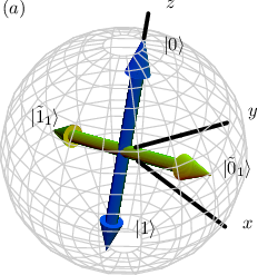

The freedom in the environment allows to write in diagonal from, whereas the freedom within the qubits allows to choose a basis in which the state can be written as
| (37) |
and still, is diagonal. To find this basis we start using the Schmidt decomposition to write
| (38) |
with being an orthonormal basis of particle . For the first qubit, we fix the axis of the Bloch sphere (containing both and ) parallel to the eigenvectors of , and the axis perpendicular (in the Bloch sphere) to both the axis and . The states contained in the plane are then real superpositions of and , which implies that and for some . In the second qubit it is enough to set and . This freedom is also related to the fact that purity only depends on . A visualization of this procedure is found in figure 5. The angle measures the entanglement () whereas the angle is related to an initial magnetization.
The general solution for purity using this parametrization is
| (39) |
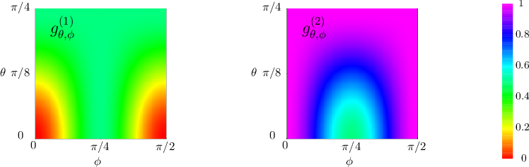
where the geometric factors , and are expressed as
| (40) | |||||
| (41) |
in terms of the functions and , defined in (21). Both geometric factors are shown in figure 6. Equation (39) is obtained from (16) and (17) by insertion of the (114) and (120) for and , respectively.
We consider again two limits for . In the degenerate limit () purity decay is given by
| (42) |
where is defined in (23). The result is independent of since a degenerate Hamiltonian is, in this context, equivalent to no Hamiltonian at all. The -dependence in this formula shows that an entangled qubit pair is more susceptible to decoherence than a separable one.
In the fast limit () we get
| (43) |
For initial states chosen as eigenstates of we find linear decay of purity both below and above Heisenberg time. In order for to be an eigenstate of it must, first of all, be a pure state (in ). Therefore this behaviour can only occur if or . Apart from that particular case, we observe in both limits, the fast as well as the degenerate limit, the characteristic linear/quadratic behaviour before/after the Heisenberg time similar to the one qubit case.

In figure 7 we show numerical simulations for . We average over 30 different Hamiltonians each probed with 45 different initial conditions. We contrast Bell states (, ) with separable states (, ), and also systems with a large level splitting () in the first qubit with systems having a degenerate Hamiltonian (). The results presented in this figure show that entanglement generally enhances decoherence. This can be anticipated from figure 6, since for fixed , increasing the value of (and hence entanglement) increases both and . At the same time we find again that increasing tends to reduce the rate of decoherence, while a strict inequality only holds among the two limiting cases (just as in the one qubit case). From , it follows that . Therefore, for fixed initial conditions and greater than 0, . This is the second aspect illustrated in figure 7.
In order to extend the formulae to longer times/smaller purities we exponentiate them using the results of C. The numerical simulations (see figure 7) agree very well with that heuristic exponentiated linear response formula. In one case (blue rhombus) where the agreement is not so perfect, we found that it is the inaccurate estimate of the asymptotic value of purity, which leads to the deviations.
4.1.2 The GOE case:
Let us consider the GOE average of both and . We have to take into consideration the weaker symmetry properties of the GOE ensemble as compared with the GUE. When averaging and over the GOE, we are again confronted with the fact that the invariance group is considerably smaller than in the GUE case. In this context the initial entanglement between the two qubits has a crucial importance since it “transports” the invariance properties from the spectator to the coupled qubit.
For the sake of simplicity, we focus on the degenerate limit setting . Note that on the basis of the results in A, the general case can be treated similarly and the corresponding result will be presented at the end of this subsection.
We first specify the operations under which the spectator Hamiltonian (32), considered as a random matrix ensemble, is invariant. As both, the internal Hamiltonian of the environment and the coupling, are selected from the GOE the invariance operations form the group
| (44) |
and have the structure , with being an orthogonal matrix (acting in ), a real number, and a unitary operator acting on the spectator qubit.
The direct product structure of the invariance group oblige us to respect the identity of each particle, but allows to analyse each qubit separately. For instance, if we would replace the random coupling matrix with one, which involves both qubits, the invariance group would be . As a consequence, purity decay would become independent of the entanglement within the qubit pair: for any entangled state one can find a orthogonal matrix which maps the state onto a separable one.
We write the initial condition as in (38). For the coupled particle follows the same analysis made in section 3.2. We can thus write and, in order to respect orthogonality, . For the second qubit we have the same complete freedom as in (4.1.1). We thus select and to erase the relative phase in the first qubit and finally write the initial state as
| (45) |
The average purity is still given by the double integral expression in (16). However, in the present case the mixed initial state must be used. For , the resulting integrand reads
| (46) |
where , and are given in (114), (120), and (124), respectively. Evaluating the double integral, we obtain
| (47) |
where is given in (30). As in the GUE case, this result depends on the entanglement of the initial state, and, as in the one-qubit GOE case, it also depends on . Again it turns out that Bell states are more susceptible to decoherence than separable states. Note however, that purity as a function of is not monotonous. Hence, a finite increase of entanglement does not guarantee that the purity decreases everywhere in time. For separable states, , we retrieve formula (29). However, for completely entangled states, , and the dependence on is lost. This is understood from a physical point of view, noticing that any bilocal unital channel (in particular unitary operations) on a Bell state can be reduced to a single local unitary operation acting on a single qubit i.e. for any local unitary operation , there exists such that
| (48) |
( is any 2 qubit pure state with , e.g. ). We can then say that the invariance properties in the second qubit are inherited from the first qubit via entanglement.
Let us obtain the standard deviation for the different possible initial conditions in the qubits. We want to analyse the situation separately for a fixed value of concurrence. Then, as the invariant measure of the ensemble of initial conditions, and fixing the amount of entanglement, we shall use the tensor product of the invariant measures in each of the qubits. Since there is no dependence of (47) on the second qubit, the appropriate invariant measure is trivially inherited from the invariant measure for a single qubit. The resulting value for the standard deviation is
| (49) |
Based on A and B we can also obtain the average purity for . The parametrization of the initial states is more complicated since two preferred directions arise, one from the eigenvectors of the internal Hamiltonian and the other from the invariance group. The result can be expressed in the form given in (16), with
| (50) |
The angle is related to a phase shift between the components of any of the eigenvectors of the initial density matrix .
4.2 The separate environment Hamiltonian
We proceed to study purity decay with other configurations of the environment. Consider the separate environment configuration, pictured in figure 1(b). The corresponding uncoupled Hamiltonian is
| (51) |
and the coupling is
| (52) |
From now on we assume that the internal Hamiltonians of the environment and the couplings are chosen from the GUE. Generalization for the GOE can be obtained along the same lines using the corresponding results of section 4.1.2. The initial condition has a separable structure with respect to both environments, see (3). Next we calculate the coupling in the interaction picture. It separates into two parts acting on different subspaces , where
| (53) |
Notice that () does not depend on (). Since and are uncorrelated quadratic averages separate as
| (54) |
This leads to a natural separation of each of the contributions to purity
| (55) |
where denotes the average purity with particle being a spectator, as given in section 4.1. In this way, the problem reduces to that of the spectator model. The respective expressions in section 4.1 may be used. For instance, if we assume broken TRI, we obtain from (39)
| (56) |
where and are the correlation functions of the corresponding environments defined in exact correspondence with (18), for and respectively. If in one or both of the qubits, the level splitting in the internal Hamiltonians is very large/small compared to the Heisenberg time in the corresponding environment (denoted by and for and , respectively) the degenerate and/or fast approximations may be used. As an example, if and we find
| (57) |
whereas if and
| (58) |
It is interesting to note that if we have two separate but equivalent environments (i.e. both Heisenberg times are equal), we get exactly the same result as for a single environment. Also notice that the Hamiltonian of the entire system separates and thus the total entanglement of the two subsystems ( and ) becomes time independent.
4.3 The joint environment configuration
The last configuration we shall consider is the one of joint environment; see figure 1(c). Its uncoupled Hamiltonian is
| (59) |
whereas the coupling is given by
| (60) |
Notice the similarity with (51) and (52). However, as discussed in the introduction, they represent very different physical situations. The coupling in the interaction picture can again be split , where
| (61) |
Note the slight difference with (53). However still and are uncorrelated, enabling us to write again (54).
From now on, the calculation is formally the same as in the separate environment case. Hence we can inherit the result (56) directly, taking into account that since they come from the same environmental Hamiltonian, the two correlation functions are the same. In case any of the Hamiltonians fulfils the fast or degenerate limit conditions, the corresponding expressions to (57) and (58) can be written. As an example, if the first qubit has no internal Hamiltonian, and the second one has a big energy difference, the resulting expression for purity decay is
| (62) |
where is the Heisenberg time of the joint environment. Monte Carlo simulations showing the validity of the result were done with satisfactory results, comparable to those obtained in figure 7. The parameter range checked was similar to that in the figure.
5 A relation between concurrence and purity
In the previous section we have found that purity decay is very sensitive to the initial degree of entanglement between the two qubits. In other words, we related the behaviour of purity in time to the degree of entanglement (measured by concurrence) at . In this section, we study the relation between purity and entanglement (again measured by concurrence) as both are evolving in time. We focus on initial states which are Bell states such that purity and concurrence are both maximal and equal to one at . Since concurrence is defined in terms of the eigenvalues of a hermitian -matrix, an analytical treatment even in linear response approximation is much more involved than in the case of purity. Instead, we work with a phenomenological relation between purity decay and concurrence discovered in [27] and further studied in [13]. It proves to be valid in a wide parameter range, and it allows to obtain an analytic prediction for concurrence decay.
We study the relation between concurrence and purity on the -plane, where we plot concurrence against purity with time as a parameter. Since the initial state is a Bell state, the starting point is always at . In this plane not all points are allowed for physical states; two constrains appear. The first one follows from the ranges of and . The second restriction follows from the “monogamy” of entanglement: if a qubit is very entangled with another qubit, it cannot be very entangled with the rest of the universe (i.e. the environment), implying some degree of purity. Conversely if the qubit is very entangled with the universe, it cannot be entangled with the other qubit. This statement can be made quantitative, which leads to the concept of maximally entangled mixed states. They define the upper bound of the set of admissible states (the corresponding area on the -plane is shown in figure 8(a) in grey). Another region of interest corresponds to those states, which form the image of a Bell state under the set of bi-local unital operations [28] (red area in the same figure). Finally, we have the Werner states , , which define a smooth curve on the -plane (black solid line). The analytic form of this curve is [13]
| (63) |
and will be referred to as the Werner curve. Note that states belonging to the Werner curve are not necessarily Werner states.


The spectator and separate environment configuration are strictly bi-local, whereas the joint environment configuration becomes bi-local in the large limit. None of the three types of environmental couplings are strictly unital. In this limit we find from our numerical simulations that all -curves fall into the region defined by the bi-local unital operations.
For figure 8(b), we perform numerical simulations of the spectator Hamiltonian assuming broken time reversal symmetry (GUE case). We compute the average purity as well as the average concurrence as a function of time. This average is over 15 different Hamiltonians and 15 different initial states for each Hamiltonian. We fix the level splitting in the coupled qubit to and consider two different values and for the coupling to the environment. figure 8(b) shows the resulting -curves for different dimensions of . Observe that for both values of , the curves converge to a certain limiting curve inside the red area (defined by the set of bi-local unital channels) as tends to infinity. While for , this curve is at a finite distance of the Werner curve, for it practically coincides with . To check this statement in more detail, consider the numerical -curve obtained from our simulations and define its distance to the Werner curve as
| (64) |
The behaviour of is shown in figure 9(a). For (black dots), the error goes to zero, which means that the corresponding -curves indeed converge to the Werner curve. In fact from a comparison with the black solid line we may conclude that the deviation is inversely proportional to the dimension of . By contrast, for (red dots), the error tends to an approximately constant value, in line with the assertion that the numerical results converge to a different curve. In figure 9(b) we plot the error as a function of , for different dimensions of as indicated in the figure legend. The results suggest that the convergence to the Werner curve occurs as long as which is of the order of for . In fact for all studied, we found a critical value such that the -curves converge to the Werner curve as long as . For all studied couplings led to convergence to the Werner curve.


In the presence of TRI the -curves again converge to the Werner curve, for values of the coupling greater than a critical value . As in the GUE case, this critical value depends on . However, in contrast to the GUE case, we find that remains finite for . In the other configurations considered (the joint and the separate environment), the behaviour is similar. In those cases it is the largest (of the two) coupling strengths which determines whether the -curves converge to the Werner curve, or not.
A partial explanation for this particular behaviour in the plane is provided in [28]. The authors find that for unital channels, the possible points in the plane that can be accessed are limited to a small 2-dimensional region, see figure 8(a).

We test the unitality of the channels induced by the non-unitary evolution in the following way. Since we want to test , we prepare an initial pure condition that leads to a completely mixed state in the qubit (let us focus on the spectator case), i.e. ,
| (65) |
with . We let the state evolve with a particular member of the ensemble of Hamiltonians defined in (1). Afterwards we evaluate the Euclidean distance of the resulting mixed state in the qubit from the fully mixed state, within the Bloch sphere. The average distance is plotted as a function of the size of the environment in figure 10. We conclude that the unitality condition is approached algebraically fast as the size of the environment increases. This by no means explains the generic accumulation to the Werner curve, but certainly restricts the possibilities; furthermore, for high purities/concurrences the area converges to the curve , hence providing a satisfactory explanation in this regime.


Sufficiently close to , the above arguments imply a one to one correspondence between purity and concurrence, which simply reads . This allows to write an approximate expression for the behaviour of concurrence as a function of time
| (66) |
using the appropriate linear response result for the purity decay. The corresponding expressions have been discussed in detail in the previous section. (66) has similar limits of validity as the linear response result for the purity. Thus, in a sense, we may call it a linear response expression for concurrence decay.
In those cases, where the coupling is beyond the critical coupling and where the exponentiated linear response expression (25) holds for the average purity, we can write down a phenomenological formula for concurrence decay, which is valid over the whole range of the decay
| (67) |
In figure 11 we show random matrix simulations for concurrence decay in the joint environment configuration. We consider small couplings which lead to the Gaussian regime for purity decay, as well as strong couplings which lead to the Fermi golden rule regime. We find good agreement with the prediction (67), except for the Gaussian regime when we switch-on a fast internal dynamics in both qubits (). These level splitting are so large, that the coupling strengths are much smaller than , which leads to the deviations observed.
Note that, in the separate environment case, the entanglement of the two subsystems defined on the spaces and is constant in time. For the initial conditions we use, the entanglement stems entirely from the two qubits. The concurrence of these two qubits decays because the constant entanglement spreads over all constituents of the two large subspaces.
6 Conclusions and outlook
We have derived general linear response formulae for the decay of purity for one and two qubits. The initial states are grouped in relevant families and the dependence on these families is analysed in detail. In particular we see that time reversal invariance will generally increase the number of families we have to consider, though entanglement will undo some of this in the two-qubit case. We do not discuss the well-known quadratic decay at very short (Zeno) times, though it obviously occurs in our model [6]. We find the linear decay resulting from the usual master equation treatment at short times, but we see the crossover to quadratic decay as we approach the Heisenberg time. This crossover is important if decoherence is dominated by a few degrees of freedom coupled to the central system, leading to a finite Heisenberg time in the relevant environment. We show that the quadratic term is absent if we choose an eigenstate of the intrinsic Hamiltonian of the central system.
In general we can say that entanglement between the qubits accelerates decoherence mainly by affecting the prefactors in the linear response expression. Internal dynamics introduces an additional term but also affects the prefactors. It tends to stabilize the system though the interplay with entanglement does not make this statement strict for small changes.
The analysis of concurrence decay and its relation to purity decay largely confirms previous findings [13, 27] in this more general setting. In particular the time-evolution follows the purity - concurrence relation of Werner states. We use this relation to give an analytic, albeit heuristic, formula for concurrence decay. Actually the relation shows small deviations for very weak couplings, and small concurrences. We obtain some understanding of these findings by showing that the process becomes unital in the limit of a large environment.
We thus have given a rather complete description of the time-evolution of decoherence and entanglement of two non-interacting qubits. From a technical point of view we find a remarkable sequence of argumentation. In linear response approximation, all two-qubit configurations can be reduced to the spectator case. This case is equivalent to a single qubit, initially in a mixed state yet not entangled with the environment. The evolution of the mixed central system is obtained in the appendix in the linear response approximation. This result in turn allows to derive the general formulae for all cases mentioned above. While this allowed a simple unified representation of the two-qubit problem in the framework of an RMT model, actually one readily suspects, that this result is more general, and this is indeed the case as we shall see in a forthcoming paper [29]. Another line, that could be easily followed, is to consider a random interaction between the two qubits and a joint coupling to the environment. While such a study is easy and has some interest, the real problem to tackle is to introduce time dependent operations such as gates, while the decoherence modelled by RMT acts. Another open problem that can be tackled in this framework is a situation of a near and far environment the first coupled weakly and the second extremely weakly. The first should probably have a finite Heisenberg time on a time scale relevant to the system, while the second more likely would have very dense spectrum and thus an infinite Heisenberg time. Finally, recall that we used formally echo dynamics for purely technical reasons. Yet this could be used to great advantage if we simultaneously want to study internal errors in the implementation of a quantum algorithm on a physical device as well as decoherence effects. As RMT is extremely successful in describing fidelity decay it seems to be the optimal approach.
Appendix A One-qubit purity decay for pure and mixed states
Here, we consider the one-qubit decoherence in a more general context. One-qubit decoherence as described in section 3 deals with a separable initial state , where is a pure state of a single qubit coupled to an environment in the pure state . We consider here arbitrary, finite dimensions of and , and we allow to be mixed. The latter poses some problems on the physical interpretation of purity as a measure for decoherence. However, these can be avoided by taking the point of view of the environment, as it becomes entangled with the central system. That means we consider the purity of the state of the environment after tracing out the central-system’s degrees of freedom; see (36). If we consider the entanglement with a spectator being responsible for the mixedness of , we can use the following results to describe purity decay in the spectator model.
In this sense, the result can be applied to the spectator model described in section 4.1.
We will derive explicit expressions for the average purity as a function of time, where the average is only over the random coupling. These expressions involve a few elemental spectral correlation functions, whose properties will be discussed in B. As detailed in section 2.4, we work with the echo operator in the linear response approximation (11). Note that is hermitian, while, due to time-order inversion, is not.
The purity of the evolving state
Let and be two density matrices, defined on the Hilbert space . We define the purity form as a function of pairs of such quantum states,
| (68) |
Since any linear operator acting on can be expanded in terms of separable operators of the form , linearity implicitly defines the purity form for arbitrary linear operators. For arbitrary operators acting both on , the purity form has the following property:
| (69) |
The purity defined in (7) can be expressed in terms of the purity form as
| (70) |
Note that on the RHS of this equation, we first take the trace over the central system, i.e. we consider the purity of the state of the environment after tracing out the central degrees of freedom. With this little twist we can describe the one-qubit decoherence in section 3 and the spectator model in section 4.1 at the same time.
Purity decay in the linear response approximation
To average purity, we use (11) to compute in linear response approximation
| (71) |
Keeping terms only up to second order in :
| (72) | |||
In the next step, we perform the ensemble average over the coupling. As a result, the terms linear in vanish. For the remaining terms, we use the properties in (69) and the fact that is hermitian, to obtain
| (73) |
In order to pull out the same double integral of and , we use the time ordering symbol . It allows to write for the average purity as a function of time
| (74) | |||
| (75) |
where and are short forms for the coupling matrices and , respectively. The arguments and of the coupling matrices are interchanged in the second and fourth term of . This does not change the value of the integral of course, but it facilitates to handle common terms in the following considerations.
The general result
The limit :
If the dimension of the Hilbert space of the environment goes to infinity, the corresponding correlation functions simplify, as discussed in B. We are then left with
| (77) |
A.1 Appendix A.1 The GUE case
The integrand in (75) consists of four terms. These terms will be considered, one after the other. We will always first average the argument of the purity form. Only then we perform the partial traces over subsystem , and therefore the final trace over the environment. The averaging is only over the coupling, and it is done by applying two simple rules, as described below.
For the coupling in the product eigenbasis of , we use either random Gaussian unitary (GUE) or orthogonal (GOE) matrices. Their statistical properties are completely characterized by the following second moments (for notational ease we ignore the subscript 1,e for a moment)
| (78) |
where if is taken from the GOE, while if is taken from the GUE. In the interaction picture we then find:
| (79) |
:
We first compute the average
| (80) |
where we have used the averaging rule, (79), as well as the fact that the time-ordering operator requests to exchange with whenever . The indices and denote basis states in , while the indices and denote basis states in . We can rewrite that expression in a more compact form by employing the diagonal matrices , defined in (105):
| (81) |
Now we apply the partial traces over subsystem
| (82) |
The final trace over the environment yields
| (83) |
:
:
We first compute the average
| (87) |
Then we apply the partial traces over subsystem
| (88) |
The final trace over the environment yields
| (89) |
:
We first compute the average
| (90) |
We apply the partial traces over subsystem
| (91) |
The final trace over the environment yields
| (92) |
A.2 The GOE case
In the GOE case, the average over the coupling yields, besides the previously considered GUE-term an additional one; see (79). In the following we will redo the calculation of the previous subsection, but consider only that additional term. As a reminder, we add the subscript 2 to the brackets which denote the ensemble average.
:
We first compute the average
| (93) |
where we have used the averaging rule, (79). Here the time-ordering operator has no effect. Now we apply the partial traces over subsystem
| (94) |
The final trace over the environment yields
| (95) |
:
:
We first compute the average
| (99) |
Then we apply the partial traces over subsystem
| (100) |
The final trace over the environment yields
| (101) |
:
We first compute the average
| (102) |
We apply the partial traces over subsystem
| (103) |
The final trace over the environment yields
| (104) |
Appendix B Some particular correlation functions relevant for the average purity decay
B.1 Definitions
Averaging over the perturbation (i.e. the coupling) leads to expressions which may involve the diagonal matrix
| (105) |
Here, denotes one of the two subsystems considered in A, either the qubit or the environment. Evidently, the energies are the eigenvalues of the corresponding Hamiltonian. In the derivations in A, the expectation value of with respect to the initial state are of particular importance. These are denoted by
| (106) |
In this work, is always a pure state.
We will also encounter another type of correlation function, which may be defined as follows
| (107) |
If the initial state is pure, this quantity becomes the return probability. At it gives the purity of . In the case of GOE averages, we also encounter the correlation function
| (108) |
B.2 Properties
The limit of infinite dimension (of ):
In the main part of this paper, we focus on the limit, where the dimension of the environment(s) becomes infinite. In that case it makes sense to perform an additional spectral average over and/or . In the case of this yields
| (109) |
where is the two-point spectral form factor with time measured in units of the Heisenberg time for the corresponding spectral ensemble. In the limit of large dimension we find for the other correlation functions:
| (110) | |||
| (111) |
For random pure states, as considered in the present work, both correlation functions are at most of order one at . For they drop very quickly and soon become of order . This happens on the same time scale, where drops from values of the order to values of the order one. In that sense we consider these correlation functions to contribute only corrections to the result given in (77).
The different correlation functions for a single qubit
A single qubit is a two level system. The most general pure initial state is given by , with . The most general mixed state is given by , with , real, , and arbitrary pure states with . We will now investigate the behaviour of the different correlation functions , and as it depends on the initial state and the Hamiltonian .
- (a)
Assume . Then
(112) holds, so
(113) - (b)
For we still have
(114) - (c)
Assume . Then we find for
(115) This expression only depends on the absolute values squared of the coefficients and . Therefore we may parametrize them without loss of generality as and . We then find
(116) - (d)
For a general mixed state we find
(117) where we have used that . Note that the coefficients may be arranged into a square unitary matrix, and must therefore be of the following general form
(118) This shows that , and that
(119) Since it is convenient to set and such that we may write and obtain
(120) - (e)
Assume again that . Then we find for
(121) However, as discussed in section 3.2, a natural symmetry around the axis (in the Bloch sphere picture) appears for . In that case, using as defined in that section, one can prove that
(122) using elementary geometric and trigonometric considerations.
- (f)
For a general mixed state we find
(123) It follows from (118) that , such that the equality holds, just as in the case of . Therefore we may write
(124) Note that the only difference to in case (d) is the additional phase in the argument of the cosine function. Using the same angle defined with (45), in complete analogy with (27), and using (122) we obtain
(125)
Appendix C The exponentiation
The linear response formulae derived throughout the article are expected to work for high purities or, equivalently, when the first two terms in the series (11) approximate the echo operator well; it is of obvious interest to extend them to cover a larger range. The extension of fidelity linear response formulae has, in some cases, been done with some effort using super-symmetry techniques. This has been possible partly due to the simple structure of fidelity, but trying to use this approach for a more complicated object such as purity seems to be out of reach for the time being. Exponentiating the formulae obtained from the linear response formalism has proven to be in good agreement with the exact super-symmetric and/or numerical results for fidelity, if the perturbation is not too big. The exponentiation of the linear response formulae for purity can be compared with Monte Carlo simulations in order to prove its validity. We wish to explain the details required to implement this procedure in this appendix.
Given a linear response formula (for which ), and an expected asymptotic value for infinite time , the exponentiation reads
| (126) |
This particular form guaranties that equals for short times, and that The particular value of will depend on the physical situation; in our case it will depend on the configuration and on the initial conditions.
Let us write the initial condition as
| (127) |
for some rotated qubits , . In each of the qubits interacting with the environment we assumed that for long enough times, the totally depolarizing channel will act (recall that the totally depolarizing channel is defined as for any density matrix ). Hence, for the spectator configuration, the final value of purity is
| (128) |
whereas for both the joint and the separate environment configuration we use the value
| (129) |
Good agreement is found with Monte Carlo simulations for moderate and strong ºcouplings.
References
References
- [1] H. Häffner, W. Hänsel, C. F. Roos, J. Benhelm, D. Chek-al-kar, M. Chwalla, T. Körber, U. D. Rapol, M. Riebe, P. O. Schmidt, C. Becher, O. Gühne, W. Dür, and R. Blatt. Scalable multiparticle entanglement of trapped ions. Nature, 438:643, December 2005.
- [2] C. A. Sackett, D. Kielpinski, B. E. King, C. Langer, V. Meyer, C. J. Myatt, M. Rowe, Q. A. Turchette, W. M. Itano, D. J. Wineland, and C. Monroe. Experimental entanglement of four particles. Nature, 404:256, Mar 2000.
- [3] Zhi Zhao, Yu-Ao Chen, An-Ning Zhang, Tao Yang, Hans J. Briegel, and Jian-Wei Pan. Experimental demonstration of five-photon entanglement and open-destination teleportation. Nature, 430:54, Jul 2004.
- [4] H. Häffner, F. Schmidt-Kaler, W. Hänsel, C. F. Roos, T. Körber, M. Chwalla, M. Riebe, J. Benhelm, U. D. Rapol, C. Becher, and R. Blatt. Robust entanglement. Applied Physics B: Lasers and Optics, 81:151, Jul 2005.
- [5] T. Gorin, T. Prosen, and T. H. Seligman. A random matrix formulation of fidelity decay. New J. Phys., 6:20, 2004.
- [6] Thomas Gorin, Tomaž Prosen, Thomas H. Seligman, and Marko Žnidarič. Phys. Rep., 435:33, 2006.
- [7] R. Schäfer, H.-J. Stöckmann, T. Gorin, and T. H. Seligman. Experimental verification of fidelity decay: From perturbative to Fermi golden rule regime. Phys. Rev. Lett., 95(18):184102, 2005.
- [8] R. Schäfer, T. Gorin, T. H. Seligman, and H.-J. Stöckmann. Fidelity amplitude of the scattering matrix in microwave cavities. New J. Phys., 7:152, 2005.
- [9] T. Gorin, T. H. Seligman, and R. L. Weaver. Scattering fidelity in elastodynamics. Phys. Rev. E, 73(1):015202(R), 2006.
- [10] W.H. Zurek. Decoherence and the transition from quantum to classical. Phys. Today, 44(10):36, 1991.
- [11] T. Gorin, T. Prosen, T. H. Seligman, and W. T. Strunz. Connection between decoherence and fidelity decay in echo dynamics. Phys. Rev. A, 70(4):042105, 2004.
- [12] T. Gorin and T. H. Seligman. A random matrix approach to decoherence. J. Opt. B, 4(4):S386, 2002.
- [13] Carlos Pineda and Thomas H. Seligman. Bell pair in a generic random matrix environment. Phys. Rev. A, 75(1):012106, 2007.
- [14] C. Pineda, private communication, 2006.
- [15] Wojciech Hubert Zurek. Decoherence, einselection, and the quantum origins of the classical. Rev. Mod. Phys., 75(3):715, May 2003.
- [16] Tomaž Prosen and Thomas H Seligman. Decoherence of spin echoes. J. Phys. A, 35(22):4707, 2002.
- [17] H.-J. Stöckmann and R. Schäfer. Fidelity Recovery in Chaotic Systems and the Debye-Waller Factor. Phys. Rev. Lett., 94(24):244101, June 2005.
- [18] T. Gorin, H. Kohler, T. Prosen, T. H. Seligman, H.-J. Stöckmann, and M. Žnidarič. Anomalous slow fidelity decay for symmetry-breaking perturbations. Phys. Rev. Lett., 96(24):244105, 2006.
- [19] G. L. Celardo, C. Pineda, and M. Žnidarič. Stability of quantum Fourier transformation on Ising quantum computer. Int. J. Quantum Inf., 3(3):441, 2005.
- [20] Èlie Cartan. Quasi composition algebras. Abh. Math. Sem. Hamburg, 11:116, 1935.
- [21] Madan Lal Mehta. Random Matrices. Academic Press, San Diego, California, second edition, 1991.
- [22] Tzu-Chieh Wei, Kae Nemoto, Paul M. Goldbart, Paul G. Kwiat, William J. Munro, and Frank Verstraete. Maximal entanglement versus entropy for mixed quantum states. Phys. Rev. A, 67(2):022110, 2003.
- [23] Florian Mintert, André R R Carvalho, Marek Kús, and Andreas Buchleitner. Measures and dynamics of entangled states. Phys. Rep., 415(4):207, 2005.
- [24] Scott Hill and William K. Wootters. Entanglement of a pair of quantum bits. Phys. Rev. Lett., 78(26):5022, 1997.
- [25] William K. Wootters. Entanglement of formation of an arbitrary state of two qubits. Phys. Rev. Lett., 80(10):2245, 1998.
- [26] Tomaž Prosen and Marko Žnidarič. Stability of quantum motion and correlation decay. J. Phys. A, 35(6):1455, 2002.
- [27] Carlos Pineda and Thomas H. Seligman. Evolution of pairwise entanglement in a coupled n-body system. Phys. Rev. A, 73(1):012305, 2006.
- [28] Mario Ziman and Vladimir Buzek. Concurrence versus purity: Influence of local channels on bell states of two qubits. Phys. Rev. A, 72(5):052325, 2005.
- [29] T. Gorin, C. Pineda, and T. H. Seligman. 2007. To be published.