The Canonical Function Method and its applications in Quantum Physics
Abstract
The Canonical Function Method (CFM) is a powerful method that solves the radial Schrödinger equation for the eigenvalues directly without having to evaluate the eigenfunctions. It is applied to various quantum mechanical problems in Atomic and Molecular physics with presence of regular or singular potentials. It has also been developed to handle single and multiple channel scattering problems where the phaseshift is required for the evaluation of the scattering cross-section. Its controllable accuracy makes it a valuable tool for the evaluation of vibrational levels of cold molecules, a sensitive test of Bohr correspondance principle and a powerful method to tackle local and non-local spin dependent problems. To submit to Rev. Mod. Phys. (2006).
pacs
03.65.-w,31.15.Gy,33.20.TpI Introduction
The Canonical Function Method (CFM) is a powerful means for solving the Radial Schrödinger Equation (RSE), a singular boundary value problem (SBVP) with a stringent dual requirement of regularity near the origin () where the potential is large and near infinity () where the potential is very small.
The CFM turns this SBVP into a regular initial value problem and allows full and accurate determination of the spectrum of the Schrödinger operator.
The CFM can handle bound states and scattering states, spinless and spin-dependent, single channel or multi-channel problems and possesses several features that makes it of interest for solving a large variety of problems in Quantum Mechanics of Atoms, Molecules and Scattering. Those capabilities are based essentially on the following main characteristics:
- •
Its capability to transform a SVBP into a regular initial value problem (RIVP), means mathematically that the CFM belongs to a family of Invariant Embedding Methods (IEM). Those essentially transform a boundary value problem into an initial value problem. The CFM is even more powerful than standard IEM techniques since it turns the nature of the problem from singular to regular.
- •
The evaluation of the Schrödinger operator spectrum is done without performing diagonalization, bypassing the evaluation of the eigenfunctions. This allows to preserve a high degree of numerical precision that is required in solving sensitive eigenvalue problems arising in Cold Molecules or large -limit problems where levels to evaluate are very close to the continuum limit or dissociation.
The numerical precision gained with the bypass of intermediate digonalization operations is reminiscent of the Golub-Reinsch algorithm (see for instance ref. Recipes) used for the singular value decomposition of arbitrary rectangular matrices.
This review is organised as follows: The next section is a description of the CFM with highlights of its mathematical aspects and its generalisation to the multichannel case. In section III the mathematical and numerical techniques of the radial Schrödinger equation are discussed and the full procedure for dealing with general potentials, energy levels and evaluation of phaseshifts is detailed in section IV. In the rest of the sections, we apply the CFM method systematically to a variety of problems highlighting its successes and showing its limitations whenever they show up. While, the versatility of the method is illustrated with the help of this selection of examples, the list below is by no means exhaustive but serves the purpose of underlining the breadth of applications of the CFM.
- •
Energy levels for regular and singular potentials (radial case)
- •
Potential estimation (in parametric or pseudo form) from spectroscopic data
- •
Test of the Bohr Correspondence Principle
- •
Vibrational energy levels of Cold Molecules and application to the molecule in the and electronic states. The Lennard-Jones molecule case is also studied.
- •
Local and Non-Local Exchange problems.
- •
Accurate Phase shift evaluation for regular and singular potentials.
In the last section before the conclusion, we treat the general but non obvious (regular and singular) 1D potentials to illustrate how the method can be applied in this case of lesser interest than the 3D’s.
In the Appendix we provide information linking the various units used since the review contains results spanning several fields of physics where different systems of units are used. The boundary conditions affecting the spectrum determination via the matching conditions at a single radial point are also discussed in the Appendix.
II The Canonical Function Method (CFM)
The CFM Kobeissi82 is a powerful means for solving the Radial Schrödinger
Equation (RSE). The mathematical difficulty of the RSE lies in the fact it is a singular boundary value
problem. The CFM turns it into a regular initial value problem and allows the full determination of the
spectrum of the Schrödinger operator bypassing the evaluation of the eigenfunctions.
The partial wave form of the RSE is written as:
| (1) |
where is the reduced mass and is the reduced probability amplitude for orbital angular momentum and eigenvalue .
The boundary conditions are:
| (2) |
The CFM developed initially by Kobeissi Kobeissi91 and his coworkers to integrate the RSE,
consists of writing the general solution representing the probability
amplitude as a function of the radial distance
in terms of two basis functions and for some energy .
Generally, the RSE is rewritten in a system of units such that
(see Appendix on units):
| (3) |
At a selected distance , a well defined set of initial conditions are satisfied by the canonical functions and their derivatives ie: with and with . Thus we write:
| (4) |
The method of solving the RSE is to proceed from simultaneously towards the origin () and towards infinity (). Expressing the continuity condition of the ”wavefunction” and its derivative at the point from the left () and right () yields (see Appendix on matching and boundary conditions):
| (5) |
When the integration is performed, the ratio of the dependent canonical functions is monitored until
saturation with respect to is reached at both limits ( and ).
The saturation of the ratio with yields a position independent
eigenvalue function .
The latter is mathematically defined with the help of two associated energy functions:
| (6) |
and:
| (7) |
as:
| (8) |
its zeroes expressing the continuity of and its derivative at the point (matching conditions) yield the spectrum of the RSE. In practice we have:
| (9) |
and:
| (10) |
with the radial coordinates where saturation is observed (within
some predefined tolerance) respectively in and .
An example of typical behaviour of is
displayed in Fig. 1. The eigenfunctions may be obtained for any
where is a zero of .

The eigenvalue function definition depends on the type of boundary conditions at hand.
In the Appendix we describe the general boundary conditions case and the corresponding
matching conditions along with the corresponding eigenvalue function.
The shape of provides a deep insight into the physical significance of the CFM method. The latter transforms a SBVP from the open interval to the finite interval defined by the saturation coordinates of the energy functions. This means the CFM maps an arbitrary potential onto the infinite square well problem defined by in the open interval and (see section VII for additional information). In fact, for the infinite square well problem has a (see also ref. Johnson).
The speed and accuracy of the CFM method have been tested and compared to standard integration algorithms such as the order four Runge-Kutta (RK4) method, Numerov etc.. in a variety of cases and for a wide of range of potentials.
More specifically, being selected as the starting point for the
integration, the -axis is divided into intervals
in a way such that the potential can be series expanded over
(see refs Fornberg1; Fornberg2).
The expansion uses coefficients so that the local
expression of the total potential is defined as:
| (11) |
In order to perform integration, we use the following variable step difference equation:
| (12) |
| (13) |
where the are a particular set of canonical functions and the are their derivatives in the interval . The are given by the recursion formula for energy obtained from series expanding eq. 3:
| (14) |
with and .
In practice, the above sums over are truncated to a cutoff value (instead of )
chosen large enough so that the remainder error is less than a selected
truncation error .
Given and , the integration step for the interval
is deduced from
.
At the starting point of integration , the starting step size is thus determined,
and the procedure is repeated at leading to and so forth
until we reach after steps.
These equations allow the propagation of the solution from one point to the next using a variable step and a local series expansion of variable order controlled by the truncation error . The accuracy of the results are monitored with respect to the decrease of and the procedure is referred to as the VSCA (Variable Step with Controlled Accuracy) method.
Generally, one avoids using or evaluating the radial wavefunction but if one insists on evaluating it, the canonical functions and are used to determine the radial wavefunction at any energy via the expression:
| (15) |
where and are the radial wavefunction and its derivative at the initial distance .
Before proceeding any further, the essential test of any method that pretends solving the RSE is the Coulomb potential and the essential case to test the accuracy and reliability of the CFM is the (textbook) Hydrogen atom.
The CFM results are shown in Table. 1 along with the exact analytical results.
| Index | CFM (Ry) | Exact (Ry) |
|---|---|---|
| 1 | -1.00000 | -1.00000 |
| 2 | -0.250000 | -0.250000 |
| 3 | -0.111111 | -0.111111 |
| 4 | -6.25000(-2) | -6.25000(-2) |
| 5 | -4.00000(-2) | -4.00000(-2) |
| 6 | -2.77778(-2) | -2.77778(-2) |
| 7 | -2.04082(-2) | -2.04082(-2) |
| 8 | -1.56250(-2) | -1.56250(-2) |
| 9 | -1.23457(-2) | -1.23457(-2) |
| 10 | -1.00000(-2) | -1.00000(-2) |
| 11 | -8.26446(-3) | -8.26446(-3) |
| 12 | -6.94444(-3) | -6.94444(-3) |
| 13 | -5.91716(-3) | -5.91716(-3) |
| 14 | -5.10204(-3) | -5.10204(-3) |
| 15 | -4.44445(-3) | -4.44445(-3) |
| 16 | -3.90625(-3) | -3.90625(-3) |
| 17 | -3.46021(-3) | -3.46021(-3) |
| 18 | -3.08642(-3) | -3.08642(-3) |
| 19 | -2.77008(-3) | -2.77008(-3) |
| 20 | -2.50000(-3) | -2.50000(-3) |
| 21 | -2.26757(-3) | -2.26757(-3) |
| 22 | -2.06612(-3) | -2.06612(-3) |
| 23 | -1.89036(-3) | -1.89036(-3) |
| 24 | -1.73611(-3) | -1.73611(-3) |
It is remarkable to notice that all digits (calculated by CFM and analytically) are
all same.
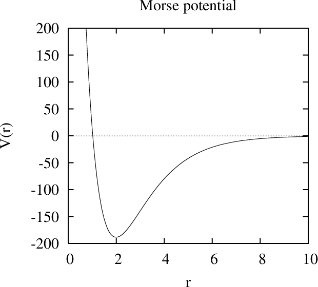
The classical Morse potential is the simplest model for the evaluation of vibrational spectra of diatomic molecules. First of all, we have analytical expressions for the levels, secondly it provides a stringent test of the CFM before embarking into more sophisticated cases such as weakly bound or cold molecules (also called long-range molecules).
The Morse potential is given by:
| (16) |
with the values equal respectively to 188.4355, 0.711248, 1.9975 in au. The analytic expression for the levels is:
| (17) |
with max . Hence the number of levels is given by: .
Working with units such that and , the Morse potential and the eigenvalue function are displayed in the figures below. The table contains the levels calculated by CFM and compared to the analytical case. Again, like in the pure Coulomb case treated previously, the agreement is perfect and we found all the levels () as predicted analytically.
| Index | CFM | Exact |
|---|---|---|
| 1 | -178.798248 | -178.798538 |
| 2 | -160.282181 | -160.283432 |
| 3 | -142.778412 | -142.78006 |
| 4 | -126.287987 | -126.288445 |
| 5 | -110.807388 | -110.808578 |
| 6 | -96.3395233 | -96.3404541 |
| 7 | -82.8832169 | -82.884079 |
| 8 | -70.4389801 | -70.4394531 |
| 9 | -59.0056 | -59.0065727 |
| 10 | -48.5851288 | -48.5854378 |
| 11 | -39.1754532 | -39.1760521 |
| 12 | -30.77771 | -30.7784157 |
| 13 | -23.3919983 | -23.3925247 |
| 14 | -17.0183048 | -17.018383 |
| 15 | -11.6557436 | -11.6559868 |
| 16 | -7.3050122 | -7.30533791 |
| 17 | -3.9661877 | -3.9664371 |
| 18 | -1.6390723 | -1.63928342 |
| 19 | -0.3238727 | -0.32387724 |

II.1 The Multichannel case
The CFM can be extended to the multichannel (or multi-component) problem, where the functions
and are no longer scalar functions of and .
Mulichannel case occurs when we have a potential well with several local minima or when
we are dealing with Scattering problems requiring simultaneously incident and
scattered wavefunctions. In addition, spin leads naturally to multicomponent wavefunctions.
Starting from a Schrödinger system of equations of the form:
| (18) |
where:
| (19) |
The elements of the matrix are physical operators and the unknown functions are partial radial waves satisfying the boundary conditions at and :
| (20) |
Following Friedman and Jamieson Friedman, we rewrite the -component equation as a set of coupled Schrödinger equations for a matrix potential with elements :
| (21) |
where .
Using linear superposition, we can write the full solution as:
| (22) |
where, as before, is an arbitrary point between zero and infinity, are independant particular solutions satisfying the set of initial conditions:
| (23) |
Going from the indicial to the matrix representation, we can build a matrix that depends on the energy and radial position defined by:
| (24) |
where and are matrices whose elements are the functions.
The analogue of the eigenvalue function is now given by the determinant equation:
| (25) |
The eigenvalues are given by the zeroes of the determinant .
Let us apply the above to the particular case where the matrix potential Friedman is a constant coupling matrix multiplying a scalar function :
| (26) |
The dependence is contained solely in the radial function
where is the scalar potential (minimum) equilibrium value.
is a full (66) constant matrix that may be diagonalised by the
similarity transformation: .
is a non-singular real constant matrix and is a (66) diagonal
matrix. Picking a coupling matrix similar to a diagonal matrix whose elements
=1..6 are respectively: , the initial
fully coupled six-channel problem 26 is transformed into six uncoupled
Schrödinger equations that are solved with the multichannel CFM. The full spectrum
of is made from the union of the sets of eigenvalues of the six individual
Schrödinger equations.
In order to benchmark the CFM results, we note that this multichannel example is nothing other than a special matrix form of the Morse potential. Then, we have access to the full spectrum analytically as in the scalar Morse case:
| (27) |
where and .
In order to perform a detailed numerical comparison between the
numerical performance of the CFM
and the multichannel Morse potential analytical results, we take:
cm-1 and Å.
The comparison between the computed and the exact eigenvalues displayed
in table 3 shows that they are almost indistinguishable.
| Exact | CFM | |
|---|---|---|
| (6,0) | -42.550 055 679 356 | -42.550 055 679 344 |
| (5,0) | -36.833 989 511 483 | -36.833 989 511 484 |
| (4,0) | -25.669 697 220 176 | -25.669 697 220 173 |
| (3,0) | -22.179 491 924 311 | -22.179 491 924 313 |
| (2,0) | -17.625 492 133 612 | -17.625 492 133 614 |
| (6,1) | -13.650 167 038 069 | -13.650 167 038 068 |
| (1,0) | -12.143 593 539 448 | -12.143 593 539 445 |
| (5,1) | -10.501 968 534 449 | -10.501 968 534 446 |
| (4,1) | -5.009 091 660 529 | -5.009 091 660 528 |
| (3,1) | -3.538 475 772 933 | -3.538 475 772 933 |
| (2,1) | -1.876 476 400 837 | -1.876 476 400 834 |
| (6,2) | -.750 278 396 781 | -.750 278 396 781 |
| (1,1) | -.430 780 618 346 | -.430 780 618 346 |
| (5,2) | -.169 947 557 416 | -.169 947 557 416 |
II.2 Evaluation of energy spectra and phaseshift
Before treating any problem with the CFM a number of constraints should be underlined in order to properly tackle any problem with this method whether it pertains to energy spectra evaluation or phaseshift:
- •
General considerations:
- –
The potential is spherically symmetric.
- –
The interval of interest should be of infinite length.
- –
Ill-conditioning and accuracy: The spectrum depends on the zeroes of . This subtraction leads to inaccuracies because the entire spectrum depends on the zeroes of in the single channel case or in the multichannel case.
- –
issue and the number of eigenvalues: The number of eigenvalues depend strongly on . should be increased until a like diagram for the energy function is obtained.
For short-range potentials, should be close to the minimum of the potential or the equilibrium value of the radial distance . If is far from minimum, it will see only those levels close to the value of .
- –
- •
Energy spectra calculations:
- –
The method being sensitive to convergence for and , One has to check that for the canonic functions and are diverging near the origin in the same way (saturation of the ratio).
- –
One has to check that for the canonic functions and have reached their Asymptotic behaviour (of the Coulombic form ).
Note: This is not true for the phase.
- –
One should have a regular structure of the type for the energy function in the single channel (or in the multichannel) case.
- –
The method is very sensitive to .
- –
Forward integration step : typically it is 0.1 to 1 in energy calculations. In phase calculations it is 0.1 to 0.01. It is sensitive to the energy used. When the energy increases the step should be decreased. There is a compromise to be reached because if the step is too much reduced any physical quantity will saturate immediately.
- –
- •
Phaseshift calculations:
- –
The phase stability might be reached long before the asymptotic regime in is reached. Typically the phase is stable when the potential is about 0.1 au.
- –
One has to check that for the canonic functions and are diverging near the origin in the same way (saturation of the ratio).
- –
The method being very sensitive to , we ought to treat separately the different types of potential. The general rules are enunciated below:
- *
Short-range potentials: Typically for all angular momentum and energies. For large energies should be reduced.
- *
Long-range potentials: Typically for all but for small energies (1-10 au). For large energies should be reduced to 0.1.
- *
- –
Bessel functions are used for Short-range potentials only. Trigonometric functions are used for Long-range and Short-range potentials potentials.
- –
Forward integration step : typically it is 0.1 to 1 in energy calculations. In phase calculations it is 0.1 to 0.01. It is sensitive to the energy used. When the energy increases the step should be decreased. There is a compromise to be reached because if the step is too much reduced any physical quantity will saturate immediately.
- –
The stability of the CFM is based on the following: two independent sets of solutions are generated at some central point, integrating inwards to the origin and outwards to the asymptotic region. Both contain linear combinations of the regular and the irregular solutions, and by suitably combining them, the irregular solution is eliminated. Integration can be made out to a very large radius, allowing the phaseshift to be determined by matching to plane or Coulomb wave solutions. It is not necessary to obtain a series expansion of the solution in order to start the integration, making it unnecessary to series expand the potential.
- –
The method can be successfully applied to scattering problems where the phaseshift is of paramount importance in the determination of the scattering cross section. Of particular importance are (e,2e) scattering problems that are dealt with in section VII.
- –
A final point to consider when dealing with the CFM using standard integration methods is that one cannot in general proceed toward the origin because of the potential singularity (for instance, the RK method blows up at ) in contrast with the VSCA algorithm.
III Potential estimation from spectroscopy
The high accuracy of the CFM allows to retrieve the potential (in parametric or pseudo form) from
the observed atomic or molecular spectra. We exploit the Quantum Defect (QD) as an
indicator of the results obtained by the CFM in order to find the optimal
parameters of the potential.
QD information is widely exploited in modern spectroscopy, to characterize
Rydberg states and in the calculation of the photoionization cross sections of various
atomic and molecular species Jungen; Aymar96.
We show in this section that QD information, used within the Distorted Wave Born
Approximation (DWBA) framework Whelan, might also prove useful for the description of
ionization processes by presenting an alternative way to account for the short
range interactions (static and exchange) in the calculation of the final state
continuum distorted waves. The range of validity of this approach reaches beyond
that Riley of the commonly used Furness-McCarthy local exchange
approximation Furness. Compared to the determination of the Hartree-Fock
non-local operator Winkler, which becomes rapidly a tedious task as the size
of the target increases, our method allows for a target-independent procedure which
can be readily applied to much larger atomic or molecular systems.
The parameters of the Green-Sellin-Zachor Green69 parametric form of the
electron-ion potential are optimized in order to reproduce the QD using the
CFM Kobeissi82. Several parametric potentials are discussed extensively
in the literature and we already used several functional forms Aymar96
adapted to different atomic systems. We have studied Tannous99 the
QD of some rare gases with the Klapisch parametric potential Klapisch71
and found that in some cases it was very difficult to optimize parameters that
provide an accurate representation of the experimental QD. We believe, the
Green-Sellin-Zachor Green69 is better suited to our present study as the parameter
space is small (two-dimensional) which allows for an efficient search of the optimized parameters.
The electron-ion potentials obtained for each Rydberg series are further modified to account classically for the electron-electron interaction in the final state. Calculations performed within the DWBA framework for the ionization of argon in the equal energy sharing geometry , which is reasonably well documented both theoretically and experimentally, clearly validate our approach and shows significant improvements over previous treatments.
III.1 Optimisation procedure
An extensive review of the applications of model potentials has been given by Hibbert Hibbert82 and Aymar et al. Aymar96. The functional form suggested by Green et al. Green69 is given by:
| with | (28) |
where and are parameters that are determined by the optimisation procedure.
The optimisation problem, at hand, is over-determined since the experimental set of energy levels
might consist of tens of values whereas the potential depends only on two
numbers, namely and . This over-determination allows us to use
several criteria for the optimisation procedure and later on select the best one
that achieves results closest to experiment.
The optimization procedure consists of defining an objective function
and finding its minimum in the two-dimensional parameter space , .
The objective function is a quadratic consisting of the difference
between some picked levels and those produced by the parametric potential through the
solution of the RSE with the CFM.
We adopted several strategies based on the following observations:
The QD value is not stable for the low levels but tends
to reach a stable value when the energy increases.
Despite the stability of the QD for the higher levels,
the experimental (and therefore) numerical accuracy decreases when
the energy increases.
Therefore a compromise should be achieved by selecting the levels in order to
define the objective function to minimize.
We found that a reasonable compromise should be based on the following operations that differ with the selected rare gas:
- 1.
Pick some level and take the average of a number of higher ones.
- 2.
Pick two high levels for which the QD has stabilised within a given accuracy.
- 3.
Pick a low level and a high one for which the QD has already stabilised.
All the above operations should yield roughly the same values for
the parameters before running the final check in order to test the
accuracy of the obtained eigenvalues.
| Series | ||
|---|---|---|
| =0 | 3.625 | 1.036 |
| =1 | 3.62 | 1.06 |
| =2 | 3.6344 | 1.036 |
The optimization program itself is based on a globally convergent
method for solving non-linear system of equations: the multidimensional
secant method developed by Broyden Broyden.
It is based on a fast and accurate method for the iterative evaluation
of the Jacobian of the objective function needed during the minimisation
procedure.
It is a Quasi-Newton method that consists of approximating the Jacobian
and updating it with an iterative procedure. It converges superlinearly
to the solution like all secant methods.
There are several ways to perform the integration of the RSE on the basis of the CFM. One may use a fixed step scheme such as the explicit RK4 method or a variable step (VSCA) procedure. Optimization wise, the RK4 method is faster than VSCA but less accurate. To judge the accuracy of our optimization we compare in table 4 our results for the energy levels and corresponding QD obtained using the RK4 and VSCA integration scheme with those of Szydlik et al. Szydlik74. The results displayed in table 4 clearly favor, as expected, the VSCA integration scheme. In contrast to the VSCA, the RK4 integration scheme is limited to fourth order accuracy. Table 4 further shows the sensitivity of the QD to the numerical values of the calculated energy levels. Despite small differences between the energy values obtained with the RK4 and VSCA methods, the corresponding QD’s largely differ. This sensitivity of the QD is the main motivation for using it rather than the raw energy levels in our optimization procedure.
| Experimental levels | RK4 | VSCA |
|---|---|---|
| -0.309522 | -0.214082 | -0.310563 |
| -0.124309 | -9.87422(-2) | -0.124506 |
| -6.76780(-2) | -5.69743(-2) | -6.76904(-2) |
| -4.25540(-2) | -3.70845(-2) | -4.25546(-2) |
| -2.92210(-2) | -2.60593(-2) | -2.92238(-2) |
| -2.13080(-2) | -1.93126(-2) | -2.13062(-2) |
| -1.62200(-2) | -1.48846(-2) | -1.62210(-2) |
| -1.27620(-2) | -1.18223(-2) | -1.27614(-2) |
| -1.03020(-2) | -9.61654(-3) | -1.03015(-2) |
| -8.49000(-3) | -7.97521(-3) | -8.49011(-3) |
| -7.11800(-3) | -6.72092(-3) | -7.11771(-3) |
| Experimental QD | RK4 | VSCA |
|---|---|---|
| 0.202561 | 0.838726 | 0.205576 |
| 0.163723 | 0.817645 | 0.165967 |
| 0.156063 | 0.810516 | 0.156415 |
| 0.152366 | 0.807174 | 0.152400 |
| 0.150046 | 0.805324 | 0.150326 |
| 0.149399 | 0.804191 | 0.149110 |
| 0.148104 | 0.803444 | 0.148345 |
| 0.148016 | 0.802940 | 0.147808 |
| 0.147664 | 0.802574 | 0.147425 |
| 0.147091 | 0.802298 | 0.147161 |
| 0.147199 | 0.802084 | 0.146957 |
IV Vibrational spectra of Cold Molecules
A new kind of high precision molecular spectroscopy is probing long-range forces between constituent atoms of molecules. This spectroscopy is based on using light to combine two colliding cold-trapped atoms into a tenuous molecule.
The burgeoning field of ”Photoassociation Spectroscopy” is allowing very precise measurement of lifetimes of the first excited states of Alkaline atoms and observation of retardation effects and long-range forces. It provides a means of probing accurately the weak interaction between these atoms Jones96.
The agreement between theory and experiment requires simultaneously a highly accurate representation of the interaction potential as well as a highly reliable method for the calculation of the corresponding energy levels.
Since our aim is directed towards the latter problem, we make use of an alternative method to evaluate the energy levels for the potential at hand instead of comparing to the experimental values in order to assess the validity of our results.
The determination of the vibrational spectra of these very tenuous molecules is extremely subtle specially for the highest levels which play an important role in photoassociation spectroscopy. Thus a careful control of accuracy is needed in order to diagonalise the Hamiltonian without losing accuracy for all energies including those close to the dissociation limit.
The magnitudes of potential energy, distance and mass values in these kinds of molecules stand several orders of magnitude above or below what is encountered in ordinary short-range molecules.
For instance, the typical intramolecular potential well depth at the equilibrium distance of about 100 (Bohrs), is a fraction of a cm-1 while the reduced mass is several 10,000 electron masses. All these extreme values require special numerical techniques in order to avoid roundoffs, divergences, numerical instability and ill-conditioning during processing.
As a first example, Johnson et al. Johnson introduced a variant of the Morse potential
with parameters given by .
While the mass parameter in the Morse case is 0.5 ,
in the Johnson case it is very large and equal to 9114.44 .
Large values of the mass parameter lead to a very shallow well
in the potential energy (see fig. 4) that means a very small
binding energy making the molecule extremely weak. This then corresponds to the so-called
long-range or cold molecule because of the extremely low molecular binding
energy. In addition the potential width around the minimum is very broad implying large
quantum fluctuations in the ground state in contrast to the ordinarily deep
and narrow Morse potential.
The potential energy is given by:
| (29) |

| Index | Exact | CFM | Johnson |
|---|---|---|---|
| 0 | 497.668182 | 497.726562 | 498. |
| 1 | 1481.66138 | 1481.67773 | 1482. |
| 2 | 2449.65503 | 2449.69922 | 2450. |
| 3 | 3401.64697 | 3401.70508 | 3402. |
| 4 | 4337.6416 | 4337.69531 | 4338. |
| 5 | 5257.63672 | 5257.68164 | 5258. |
| 6 | 6161.63232 | 6161.66016 | 6162. |
| 7 | 7049.62842 | 7049.63672 | 7050. |
| 8 | 7921.62256 | 7921.67969 | 7922. |
| 9 | 8777.62012 | 8777.70508 | 8778. |
| 10 | 9617.61719 | 9617.67578 | 9618. |
| 11 | 10441.6133 | 10441.6348 | 10442. |
| 12 | 11249.6113 | 11249.6504 | 11250. |
| 13 | 12041.6084 | 12041.6914 | 12042. |
| 14 | 12817.6074 | 12817.6465 | 12818. |
| 15 | 13577.6055 | 13577.6445 | 13578. |
| 16 | 14321.6045 | 14321.666 | |
| 17 | 15049.6045 | 15049.6191 | |
| 18 | 15761.6035 | 15761.666 | |
| 19 | 16457.6035 | 16457.6484 | |
| 20 | 17137.6055 | 17137.6523 | |
| 21 | 17801.6055 | 17801.6484 | |
| 22 | 18449.6074 | 18449.6328 | |
| 23 | 19081.6094 | 19081.6562 | |
| 24 | 19697.6113 | 19697.6406 | |
| 25 | 20297.6152 | 20297.666 | |
| 26 | 20881.6172 | 20881.6562 | |
| 27 | 21449.6211 | 21449.6602 | |
| 28 | 22001.625 | 22001.668 | |
| 29 | 22537.6289 | 22537.6328 |
In order to perform the eigenvalue calculation we rescale the parameters such that they are as close as possible to the Morse potential described previously. The scaling yields the parameters: These values yield in a straightforward way all the eigenvalues (62 in total), the first thirty only being displayed in Table 7.
IV.1 Vibrational energy levels of the molecule
Since vibrational spectra of the Johnson molecule is determined accurately and to arbitrary accuracy with the CFM, we move on to tackle the molecule. The energy levels of the and electronic states of the molecule are determined from the Ground state up to the continuum limit. The method is validated by comparison with previous results obtained by Stwalley et al. Stwalley78 using the same potential and Trost et al. Trost98 whose work is based on the Lennard-Jones potential adapted to long-range molecules.
The method we use in this work adapts well to this extreme situation with the proviso of employing a series of isospectral scaling transformations we explain below.
We apply the CFM to the calculation of the vibrational energy levels of a diatomic molecule where the interaction between the atoms is given by the Movre and Pichler potential Movre77.
We start with the electronic state of the molecule. The corresponding potential is given by:
| (30) |
where .
is the internuclear distance and the parameter is such that:
| (31) |
Identification of the large limit yields the result: . In the calculations below, we have used Hartrees. like Stwalley et al.Stwalley78. The parameter Rydbergs is the atomic spin-orbit splitting. Given and , the equilibrium internuclear distance is .
The peculiarities of the and electronic states of the molecule are evident in fig. 5. The state is higher that the and the number of vibrational levels is smaller because the potential is shallower. This has important consequences as we we explore the vibrational spectrum below.


We scale all energies with a factor (usually cm-1) with the use of equation (1). Then we scale all distances with a typical length transforming the RSE appropriately. This double transformation is reflected generally in the potential coefficients preserving thus the functional form of the potential.
In order to gauge the accuracy of the spectra, we perform the integration of the RSE with two different methods: the fixed step RK4 and the variable step VSCA methods Kobeissi91.
The VSCA method is based on a series expansion of the potential and the corresponding solution to an order such that a required tolerance criterion is met. Ideally, the series coefficients are determined analytically to any order, otherwise loss of accuracy occurs leading quickly to numerical uncertainties as discussed later.

Table 8 shows the results we obtain with the RK4 method. The limitation of the RK4 method to fourth order hampers the finding of levels beyond the 33rd (see table 8). In order to find the higher levels we have to select an algorithm that enables us to tune the accuracy well beyond the fourth order.
Pushing the accuracy within the framework of a fixed step method has the effect of reducing substantially the integration step. In order to avoid this problem, we use a variable step that adjusts itself to the desired accuracy, the VSCA method.
This method is powerful and flexible enough to find all the desired energy levels and allows us to find one additional level that was not detected before. It should be noted that the last three levels given by Stwalley at al. Stwalley78 were extrapolated and not calculated. The agreement between our calculated levels and those of Stwalley et al. Stwalley78 is quite good. We believe that the small discrepancy, increasing as we progress towards the dissociation limit, is due to a loss of accuracy associated with traditional methods in sharp contrast with the CFM.
| Index | RK4 (cm-1) | Stwalley et al. (cm-1) | Ratio |
|---|---|---|---|
| 1 | -1.7864563 | -1.7887 | 1.00126 |
| 2 | -1.5595812 | -1.5617 | 1.00136 |
| 3 | -1.3546211 | -1.3566 | 1.00146 |
| 4 | -1.1704091 | -1.1723 | 1.00162 |
| 5 | -1.0057168 | -1.0075 | 1.00177 |
| 6 | -0.8592746 | -0.86087 | 1.00186 |
| 7 | -0.7297888 | -0.73125 | 1.00200 |
| 8 | -0.6159592 | -0.61729 | 1.00216 |
| 9 | -0.5164938 | -0.51770 | 1.00234 |
| 10 | -0.4301231 | -0.43120 | 1.00250 |
| 11 | -0.3556114 | -0.35657 | 1.00270 |
| 12 | -0.2917683 | -0.29261 | 1.00288 |
| 13 | -0.2374567 | -0.23820 | 1.00313 |
| 14 | -0.1916004 | -0.19224 | 1.00334 |
| 15 | -0.1531898 | -0.15374 | 1.00359 |
| 16 | -0.1212858 | -0.12176 | 1.00391 |
| 17 | -9.5022481(-02) | -9.5438(-02) | 1.00437 |
| 18 | -7.3608067(-02) | -7.3940(-02) | 1.00451 |
| 19 | -5.6325397(-02) | -5.6599(-02) | 1.00486 |
| 20 | -4.2530440(-02) | -4.2754(-02) | 1.00526 |
| 21 | -3.1650256(-02) | -3.1831(-02) | 1.00571 |
| 22 | -2.3180032(-02) | -2.3323(-02) | 1.00617 |
| 23 | -1.6679434(-02) | -1.6791(-02) | 1.00669 |
| 24 | -1.1768423(-02) | -1.1854(-02) | 1.00727 |
| 25 | -8.1226859(-03) | -8.1873(-03) | 1.00795 |
| 26 | -5.4687973(-03) | -5.5165(-03) | 1.00872 |
| 27 | -3.5792655(-03) | -3.6136(-03) | 1.00959 |
| 28 | -2.2675456(-03) | -2.2916(-03) | 1.01061 |
| 29 | -1.3831324(-03) | -1.3995(-03) | 1.01183 |
| 30 | -8.0680818(-04) | -8.1747(-04) | 1.01321 |
| 31 | -4.4611287(-04) | -4.5276(-04) | 1.01490 |
| 32 | -2.3077899(-04) | -2.3503(-04) | 1.01842 |
| 33 | -9.4777816(-05) | -1.1252(-04) | 1.18720 |
| 34 | -4.8564(-05) | ||
| 35 | -1.8262(-05) | ||
| 36 | -5.6648(-06) | ||
| 37 | -1.3175(-06) | ||
| 38 | -1.9247(-07) | ||
| 39 | -1.1215(-08) | ||
| 40 | -4.1916(-11) |
| Index | Stwalley et al. (cm-1) | VSCA (cm-1) | Ratio |
|---|---|---|---|
| 1 | -1.7887 | -1.7864488 | 1.00126 |
| 2 | -1.5617 | -1.5595638 | 1.00137 |
| 3 | -1.3566 | -1.3546072 | 1.00147 |
| 4 | -1.1723 | -1.1703990 | 1.00162 |
| 5 | -1.0075 | -1.0057071 | 1.00178 |
| 6 | -0.86087 | -0.8592631 | 1.00187 |
| 7 | -0.73125 | -0.7297908 | 1.00200 |
| 8 | -0.61729 | -0.6159534 | 1.00202 |
| 9 | -0.51770 | -0.5164882 | 1.00235 |
| 10 | -0.43120 | -0.4301217 | 1.00251 |
| 11 | -0.35657 | -0.3556148 | 1.00269 |
| 12 | -0.29261 | -0.2917693 | 1.00288 |
| 13 | -0.23820 | -0.2374560 | 1.00313 |
| 14 | -0.19224 | -0.1916002 | 1.00334 |
| 15 | -0.15374 | -0.1531893 | 1.00359 |
| 16 | -0.12176 | -0.1212854 | 1.00391 |
| 17 | -9.5438(-02) | -9.5022588(-02) | 1.00437 |
| 18 | -7.3940(-02) | -7.3608452(-02) | 1.00450 |
| 19 | -5.6599(-02) | -5.6325744(-02) | 1.00485 |
| 20 | -4.2754(-02) | -4.2530867(-02) | 1.00525 |
| 21 | -3.1831(-02) | -3.1650591(-02) | 1.00570 |
| 22 | -2.3323(-02) | -2.3180420(-02) | 1.00615 |
| 23 | -1.6791(-02) | -1.6679756(-02) | 1.00667 |
| 24 | -1.1854(-02) | -1.1768655(-02) | 1.00725 |
| 25 | -8.1873(-03) | -8.1228816(-03) | 1.00793 |
| 26 | -5.5165(-03) | -5.4689541(-03) | 1.00869 |
| 27 | -3.6136(-03) | -3.5793742(-03) | 1.00956 |
| 28 | -2.2916(-03) | -2.2676168(-03) | 1.01058 |
| 29 | -1.3995(-03) | -1.3831806(-03) | 1.01180 |
| 30 | -8.1747(-04) | -8.0683859(-04) | 1.01318 |
| 31 | -4.5276(-04) | -4.4613249(-04) | 1.01486 |
| 32 | -2.3503(-04) | -2.3110168(-04) | 1.01700 |
| 33 | -1.1252(-04) | -1.1035443(-04) | 1.01962 |
| 34 | -4.8564(-05) | -4.7468345(-05) | 1.02308 |
| 35 | -1.8262(-05) | -1.7767388(-05) | 1.02784 |
| 36 | -5.6648(-06) | -5.4747950(-06) | 1.03471 |
| 37 | -1.3175(-06) | -1.2597092(-06) | 1.04588 |
| 38 | -1.9247(-07) | -1.2716754(-07) | 1.51352 |
| 39 | -1.1215(-08) | ||
| 40 | -4.1916(-11) |
| Index | RK4 (cm-1) | Stwalley et al.(cm-1) | Ratio |
|---|---|---|---|
| 1 | 0.1319536 | 0.13212 | 1.00126 |
| 2 | 9.0057392(-02) | 9.0192(-02) | 1.00149 |
| 3 | 5.9472159(-02) | 5.9574(-02) | 1.00171 |
| 4 | 3.7821597(-02) | 3.7896(-02) | 1.00197 |
| 5 | 2.3027828(-02) | 2.3080(-02) | 1.00227 |
| 6 | 1.3324091(-02) | 1.3359(-02) | 1.00262 |
| 7 | 7.2562182(-03) | 7.2787(-03) | 1.00310 |
| 8 | 3.6714971(-03) | 3.6849(-03) | 1.00365 |
| 9 | 1.6950002(-03) | 1.7024(-03) | 1.00437 |
| 10 | 6.9533077(-04) | 6.9904(-04) | 1.00533 |
| 11 | 2.4102039(-04) | 2.4492(-04) | 1.01618 |
| 12 | 6.8430(-05) | ||
| 13 | 1.3446(-05) | ||
| 14 | 1.4122(-06) | ||
| 15 | 3.8739(-08) | ||
| 16 | 1.2735(-12) |
| Index | Stwalley et al. (cm-1) | VSCA (cm-1) | Ratio |
|---|---|---|---|
| 1 | 0.13212 | 0.13244150 | 1.00243 |
| 2 | 9.0192(-02) | 9.07598688(-02) | 1.00630 |
| 3 | 5.9574(-02) | 6.01645742(-02) | 1.00991 |
| 4 | 3.7896(-02) | 3.83982868(-02) | 1.01325 |
| 5 | 2.3080(-02) | 2.34584275(-02) | 1.01640 |
| 6 | 1.3359(-02) | 1.36187753(-02) | 1.01944 |
| 7 | 7.2787(-03) | 7.44243743(-03) | 1.02250 |
| 8 | 3.6849(-03) | 3.77999552(-03) | 1.02581 |
| 9 | 1.7024(-03) | 1.75281307(-03) | 1.02961 |
| 10 | 6.9904(-04) | 7.23013793(-04) | 1.03430 |
| 11 | 2.4492(-04) | 2.54856605(-04) | 1.04057 |
| 12 | 6.8430(-05) | 7.18249908(-05) | 1.04961 |
| 13 | 1.3446(-05) | 1.43120199(-05) | 1.06441 |
| 14 | 1.4122(-06) | 1.53931042(-06) | 1.09001 |
| 15 | 3.8739(-08) | 4.66022073(-09) | |
| 16 | 1.2735(-12) |
The estimation of accuracy of the results hinges basically
on two operations, integration and determination of the zeroes
of the eigenvalue function . The superiority of the VSCA
method is observed in the determination of the upper levels that are
not detected by the RK4 method (see Tables 1 and 2).
In addition, it is observed in the behavior of the eigenvalue ratio
versus the index. While in both cases (RK4 and VSCA) the ratio increases steadily as
the index increases because we are probing higher excited states, in the
RK4 case it rather blows up as dissociation is approached. We use typically
series expansion to order 12 in VSCA with a tolerance of .
In the root search of , the tolerance required for a zero
to be considered as an eigenvalue is .
This does not imply that we disagree as strongly as 0.13%, for instance,
with the Ground state value (see Tables 1 and 2) found by Stwalley et al.
Stwalley78 for the simple reason, we use a splitting energy
Rydbergs corresponding to an equilibrium
internuclear distance .
Stwalley et al. do not provide explicitly the value of they use,
however Jones et al. Jones96 use a value that is slightly
different.
We move on to treat the electronic state of the molecule. The potential associated with the electronic state of the molecule is a lot more involved. Its VSCA implementation is particularly difficult because of the complex functional of the potential as we explain below. Analytically, the VSCA algorithm requires performing a Taylor series expansion to any order around an arbitrary point Kobeissi90.
Numerically, this is still an open problem for arbitrary functions. If one turns toward the use of LISP based symbolic manipulation techniques cumbersome expressions are produced hampering any progress. Special methods based on analytical fitting expressions are needed in order to turn the series coefficients into a more manageable form (see refs Fornberg1; Fornberg2).
The first step is to determine the electronic state of the molecule by solving the Movre et al. Movre77 secular equation such that:
| (32) |
where and . In addition, , and .
The parameter is such that:
| (33) |
Identification of the large limit yields to the result: . We have used in the calculations below =1.383 Hartrees. like Stwalley et al. The parameter Rydbergs is the same as for the state.
Table 4 displays the results we obtain with the RK4 method that cannot find more than 11 levels due to accuracy limitations.

The next results for the electronic state of the molecule are obtained with the VSCA method as shown in table 5. We find an additional 15-th level in contrast to Stwalley et al. who found fourteen and extrapolated the last two levels.
The corresponding graph of the eigenvalue function is displayed in
Fig. 6 below.
IV.2 Lennard-Jones molecules
We apply our methodology to the Lennard-Jones case. Our results are compared to the results obtained by Trost et al. Trost98. We start with the levels obtained with the RK4 method. The energy unit is the absolute value of potential well depth. The Asymmetric Lennard-Jones potential (ALJ) is given by:
| (34) |
It depends on and that yield an equilibrium distance at and a potential depth . In order to compare with the appropriate litterature, Trost et al. Trost98 use rather the general parameterisation:
| (35) |
It is scaled in such a way that the energy is expressed in units of the
potential well depth . When , we obtain
and . and the radial distance is in
where is a reduced scaled mass given by . Numerically Trost et al. use which
is the order of magnitude encountered in long-range molecules within
the framework of their system of units.
The potential energy in these units is displayed in Fig. 7.
The RK4 methods yields the results displayed in Table 6.
The accuracy limitation of the RK4 results in losing the uppermost level 24. Thus we move on to the results obtained with the superior VSCA method. All levels are obtained with the VSCA and the agreement with Trost et al. results is perfect as witnessed by the ratio values of Table 6. The eigenvalue function obtained with the VSCA method as a function of energy is displayed in Fig. 8.
V Test of Bohr Correspondance Principle
LeRoy and Bernstein LeRoy70 used a WKB approximation to derive a semi-classical
formula (SCF) for the distribution
of vibrational levels near the dissociation limit of diatomic molecules. If the long-range
interatomic potential is of the form their formula allows the determination of
the dissociation energy as well as the tail of the potential ( and ) from the
experimental energies of the highest vibrational levels. Furthermore, this analysis opens
the possibility of testing directly Bohr Correspondence Principle (BCP) that states
the agreement between semi-classical
and quantum results improves for larger quantum numbers.
We consider the rotationless (L=0) and the electronic states of the molecule
correlating asymptotically to the atomic and states. The interaction between the
atoms is represented by the Movre-Pichler Movre77 potential that behaves as as
and we use the same parameters as those of Stwalley et al. Stwalley78.
The Asymmetric Lennard-Jones potential (ALJ) is also considered in
the highly unsymmetric case (we tackle here the case and ,
therefore we have asymptotically ) and the Trost et al. Trost98 case.
Both potentials are tailored to the study of Long-range molecules.
The determination of the vibrational spectra of these very tenuous molecules
is extremely subtle especially for the highest levels which play an important role in photoassociation
spectroscopy. Special care is needed in order to diagonalise the Hamiltonian without losing
accuracy for all energies including those close to the dissociation limit.
The magnitudes of potential energy, distance and mass values in this kind of molecules stand several
orders of magnitude above or below what is encountered in ordinary short-range molecules. For instance the typical intramolecular
potential well depth at the equilibrium distance of about 100 (Bohrs), is a
fraction of a cm-1 while the reduced mass is several 10,000 electron masses as
observed in the Johnson case previously. All these
extreme values require special numerical techniques in order to avoid roundoffs, divergences,
numerical instability and ill-conditioning during processing.
Accuracy and its control being of paramount importance in this work, the CFM Kobeissi82 is an excellent candidate because it bypasses the calculation of the eigenfunctions. This avoids losing accuracy associated with the numerical calculation specially with rapidly oscillating wave functions of highly excited states close to the dissociation limit.
The semi-classical approximation has been already discussed in the literature Boisseau98; Trost98. Here we refer to the original LeRoy and Bernstein formulation.
The next section is a discussion of the the Semi-classical analysis as formulated by LeRoy and Berstein with its implications. We present further the results we obtain for the vibrational levels of the molecule and electronic states. We present an additional validation of the method with the ALJ molecular potential.
V.1 Semi-classical analysis
The derivation of the LeRoy and Bernstein LeRoy70 SCF is based on the WKB condition for the eigenvalues of a potential :
| (36) |
where is the reduced mass, is the energy of the level indexed by and
are the the corresponding classical turning points.
Near the dissociation limit, one considers as a continuous function of and by differentiation of eq. (36) one obtains:
| (37) |
Using the asymptotic expression of and changing the variable of integration to , we obtain:
| (38) |
This integral can be expressed in terms of incomplete Euler Beta functions we use to check the accuracy and validate the results. LeRoy and Bernstein LeRoy70 SCF is derived by taking the limit which leads to:
| (39) |
| Index | RK4 | Trost et al. | Ratio |
|---|---|---|---|
| 1 | -0.9410450 | -0.9410460 | 1.000001 |
| 2 | -0.8299980 | -0.8300020 | 1.000005 |
| 3 | -0.7276400 | -0.7276457 | 1.000008 |
| 4 | -0.6336860 | -0.6336930 | 1.000011 |
| 5 | -0.5478430 | -0.5478520 | 1.000017 |
| 6 | -0.4698130 | -0.4698229 | 1.000021 |
| 7 | -0.3992870 | -0.3992968 | 1.000025 |
| 8 | -0.3359470 | -0.3359561 | 1.000027 |
| 9 | -0.2794670 | -0.2794734 | 1.000023 |
| 10 | -0.2295070 | -0.2295117 | 1.000021 |
| 11 | -0.1857220 | -0.1857237 | 1.000009 |
| 12 | -0.1477510 | -0.1477514 | 1.000003 |
| 13 | -0.1152270 | -0.1152259 | 0.999990 |
| 14 | -8.776970(-02) | -8.7766914(-02) | 0.999968 |
| 15 | -6.498640(-02) | -6.4982730(-02) | 0.999944 |
| 16 | -4.647400(-02) | -4.6469911(-02) | 0.999912 |
| 17 | -3.181750(-02) | -3.1813309(-02) | 0.999868 |
| 18 | -2.059000(-02) | -2.0586161(-02) | 0.999814 |
| 19 | -1.235370(-02) | -1.2350373(-02) | 0.999731 |
| 20 | -6.659580(-03) | -6.6570240(-03) | 0.999616 |
| 21 | -3.048890(-03) | -3.0471360(-03) | 0.999425 |
| 22 | -1.053690(-03) | -1.0527480(-03) | 0.999106 |
| 23 | -1.645210(-04) | -1.9834000(-04) | 1.205560 |
| 24 | -2.6970000(-06) |
| Index | VSCA | Trost et al. | Ratio |
|---|---|---|---|
| 1 | -0.9410443 | -0.9410460 | 1.000002 |
| 2 | -0.8299963 | -0.8300020 | 1.000007 |
| 3 | -0.7276415 | -0.7276457 | 1.000006 |
| 4 | -0.6336915 | -0.6336930 | 1.000002 |
| 5 | -0.5478480 | -0.5478520 | 1.000007 |
| 6 | -0.4698206 | -0.4698229 | 1.000005 |
| 7 | -0.3992947 | -0.3992968 | 1.000005 |
| 8 | -0.3359533 | -0.3359561 | 1.000008 |
| 9 | -0.2794718 | -0.2794734 | 1.000005 |
| 10 | -0.2295109 | -0.2295117 | 1.000003 |
| 11 | -0.1857222 | -0.1857237 | 1.000008 |
| 12 | -0.1477498 | -0.1477514 | 1.000010 |
| 13 | -0.1152247 | -0.1152259 | 1.000010 |
| 14 | -8.7766358(-02) | -8.7766914(-02) | 1.000006 |
| 15 | -6.4982534(-02) | -6.4982730(-02) | 1.000003 |
| 16 | -4.6469838(-02) | -4.6469911(-02) | 1.000002 |
| 17 | -3.1813146(-02) | -3.1813309(-02) | 1.000005 |
| 18 | -2.0585953(-02) | -2.0586161(-02) | 1.000010 |
| 19 | -1.2350173(-02) | -1.2350373(-02) | 1.000016 |
| 20 | -6.6568735(-03) | -6.6570240(-03) | 1.000023 |
| 21 | -3.0470500(-03) | -3.0471360(-03) | 1.000028 |
| 22 | -1.0526883(-03) | -1.0527480(-03) | 1.000057 |
| 23 | -1.9832170(-04) | -1.9834000(-04) | 1.000092 |
| 24 | -2.6957891(-06) | -2.6970000(-06) | 1.000449 |
where is a constant we calculate below for n=3 and n=6. Integrating the above equation yields:
| (40) |
where is the uppermost vibrational level index and is generally not an integer that depends on interactions having shorter range LeRoy70; Stwalley78.
Taking the origin of energies at the dissociation limit and following Gao Gao99, we define a length scale with:
| (41) |
This length should be larger than any length scale encountered in the system. In the case n=3, one defines a dimensionless bound-state energy by the scaling:
| (42) |
With the use of eq. (40) this leads to:
| (43) |
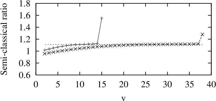
This implies that the spacing between two scaled neighbouring vibrational levels taken to power (1/6) is a universal constant given by numerically equal to 1.11292.
In the Lennard-Jones and the Trost et al. cases (n=6), the scaled bound-state energy takes the form:
| (44) |
Proceeding like the previous case, eq. (40) leads to:
| (45) |
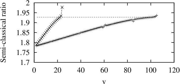
In this case, the spacing between two scaled neighbouring vibrational levels taken to power (1/3) is given by numerically equal to 1.92763. Thus, one has to determine the vibrational levels and examine the limit of as increases.
V.2 Test with the molecule
We apply the CFM to the calculation of the vibrational energy levels of a
diatomic molecule where the interaction between the atoms is given by the Movre and Pichler
potential Movre77; Jones96.
After scaling all energies with a factor (usually cm-1) and all distances with a typical
length the potential coefficients in the RSE are transformed in a way such that
the functional form of the potential is preserved.
The eigenvalue function depicted in fig. 10 shows that the shape is observed again indicating that the CFM is able to perform accurately as previously despite the extreme sensitivity of this problem.

The integration of the RSE is performed with the VSCA method
Kobeissi91. This method is superior to fixed step methods and is based on a series
expansion of the potential and the corresponding solution to an order such that a required
tolerance criterion is met. Ideally, the series coefficients are determined analytically to
any order, otherwise loss of accuracy occurs leading quickly to numerical uncertainties.
This method is powerful and flexible enough to find all the sought levels plus additional
levels not detected before by Stwalley et al. Stwalley78. It should be noted that
the last three levels given by
Stwalley at al. Stwalley78 were extrapolated and not calculated. The agreement
between the rest of our own calculated levels and those of Stwalley et al. is quite good.
We find all sought levels plus an additional level that was not detected before.
The agreement between our calculated levels and those of Stwalley et al. Stwalley78
turns out to be very good.
The semi-classical analysis is displayed in Fig. 9. It shows clearly that the sequence of Vibrational levels approaches the semi-classical limit 1.11292. The departure from this limit at the uppermost side of the spectrum is stronger for the than for the state. A crossover region is spanned by the semi-classical limit and appears to be narrower for the than for the case.
V.3 Test with Lennard-Jones molecules
We apply our methodology to the Asymmetric Lennard-Jones case (ALJ) as considered by Trost et al. Trost98. After obtaining good agreement between the CFM eigenvalues and Trost et al.’s we display the results of the semi-classical analysis in Fig. 6. The sequence of neighbouring levels approaches the theoretical limit 1.92763. The departure from this limit at the uppermost side of the spectrum is stronger for the Trost case than for the ALJ case and the width of the crossover region is almost zero in the Trost et al. case.
Gao Gao99 applied this analysis to sequences of neighbouring levels with his own
calculated levels and claimed that BCP breaks down for all quantum systems in which the asymptotic
interaction is of the form with .
Additionally Gao found that the agreement between his calculated levels and the SCF is better around the middle of the vibrational spectra contrary to Stwalley et al.’s Stwalley78 and our work.
Fig. 2 clearly shows that the semi-classical limit is reached as we increase the quantum number for the and states of the molecule. The departure is obtained with the levels we obtained at the high end of the spectra with the VSCA method based on the CFM. The crossover region is wider in the case and the departure is smaller.
On the other hand, Fig. 3 pertaining to the Lennard-Jones () case shows that
the crossover region is quite narrow for the ALJ as well as the Trost et al. case in comparison
with the case. The departure is also stronger in the Trost case.
Additional work is needed is order to tie the width of the crossover region
to the asymptotic character of the potential.
VI Exchange: local and non-local
Calculations of cross sections for photoionisation require the resolution of the integro-differential equations satisfied by the radial parts of the free electron wavefunctions. Very often a simplifying approximation is made through replacement of the exchange operator by a central equivalent exchange potential (Furness and McCarthy Furness, Bransden and Noble Bransden). While this is probably satisfactory for electrons with energies of a few eV and more it may cause problems near to threshold. Furthermore, to interpret the new generation of experiments using polarized electrons the proper inclusion of exchange may well be important. There exists a means of exact solution of the equation for the radial wavefunction including static and static-exchange terms (the diagonal parts of the direct potential and the exchange operator) and a polarisation potential. This is the Distorted Wave Polarised Orbital (DWPO) method of McDowell et al McDowella which was developed for Distorted Wave Born calculations of excitation of Hydrogen (McDowell et al McDowellb) and of Helium Scott and replaces the integro-differential equation by coupled differential equations. In both cases, only an s-state of the atom is considered and the central potentials are expressed in analytical form.
The phaseshift and the wavefunction in the asymptotic region were determined by use of the analytic second order JWKB solution (Burgess Burgess). The solutions are started by means of series expansions at the origin and continued by Numerov Numerov integration: the form of series corresponding to the regular solution is imposed by taking a power at the origin in the partial wave. For small the choice of integration step and changeover point is delicate, since convergence of the series requires small r whereas the Numerov integration becomes unstable (picking up some of the irregular solution) if it is started at too small a radius.
Accuracy in evaluating the scattering phaseshift produced in electron atom collisions
is demanded in order to estimate reliably the cross section Raw.
In (e, 2e) Whelan
collision type experiments, triple Differential Cross
Sections (TDCS) for electron impact ionization of an atom or ion, estimated within
the Distorted Wave Born Approximation (DWBA), are required.
Computational difficulties such as instabilities, lack of accuracy or convergence slow-down
arise in solving the corresponding Schrödinger equation. The latter has to respect Pauli exclusion
principle stating that the wave function of the incident electron be anti-symmetric with the wave
functions of the electrons in the target atom or molecule. In the
Hartree-Fock formulation, this requirement leads to the presence of non local
terms in the resulting coupled differential equations satisfied by the radial parts of the free
electron wavefunctions Raw; Whelan. The non-local kernel of the integro-differential
type equation originating from the exchange operator is often simplified and
a central LEE potential is used or some decoupling
procedure is employed Henry. A review of the different methods to treat
this problem on the basis of the Lippman-Schwinger equation is given
by Rawitscher et al. Raw.
Furness and McCarthy Furness and Bransden and Noble Bransden cover the
DWBA aspects.
Using a local exchange potential approximation is probably satisfactory for
electrons with energies of a few eV and
more, however it may cause problems near to threshold. On the other hand,
the interpretation of experiments using polarized electrons, requires
proper account for exchange. In addition, it is worthwhile to
develop a version of the DWBA Whelan including
non-local exchange and applicable to heavy atom targets.
This stems from the fact, the
successful Converged Close Coupling (CCC) approach of Bray Bray
becomes increasingly difficult to apply as target complexity increases.
The Distorted Wave Polarised Orbital (DWPO) method is a means
for extracting the exact solution of
the radial wave equation with static, static-exchange
terms (the diagonal parts of the direct potential and the exchange operator)
and some polarisation potential. It has been developed by
McDowell et al McDowella for DWBA
calculations for the ionization of Hydrogen (McDowell et al
McDowellb) and of Helium Scott. It replaces the integro-differential
equation by coupled differential equations. Only an s-state of
the Hydrogen or Helium atoms is considered and the central potentials are
expressed in analytical form.
The phaseshift and the wavefunction in the asymptotic region are determined
by use of the analytic second order JWKB solution (Burgess Burgess). If the
energy of the free electron is Ry, the integro-differential
equation can be rewritten in terms of the variable but the
value of the radius out to which exchange and the short-range part of the
static potential remain significant, is determined by the extent of the electron
cloud of the atom. For small , the second order JWKB solution is valid only
at radii very much larger than that of the asymptotic zone where
exchange and short-range potentials are negligible.
VI.1 The integro-differential equation
We consider the impact of a free electron of energy Ry on a one-electron atomic system of nuclear charge in a atomic state of energy Ry with a radial wavefunction . For a free electron with angular momentum quantum numbers , if we include only on-diagonal potentials and exchange operators and replace the neglected off-diagonal coupling potentials by a polarisation potential , its radial wavefunction satisfies the integro-differential equation:
| (46) |
where:
| (47) |
and:
| (48) |
This integro-differential equation can be transformed into the following system of coupled differential equations, which is the starting point for McDowell et al McDowella; McDowellb:
| (49) |
where
| (50) |
is a term appearing for the special case of zero orbital momentum (). is the Kronecker delta and
| (51) |
Our aim is to solve this system subject to the boundary conditions McDowella; McDowellb for the Hartree functions:
| (52) | |||||
where is a normalisation factor, is the phaseshift for specific and and are respectively:
- •
multiplied spherical Bessel and Neumann functions when (so that is a short range potential falling off faster than as tends to infinity);
- •
regular and irregular Coulomb wavefunctions when (so that is a long range potential behaving like when tends to infinity).
In the more general case of an ion with a frozen core and an outer shell of electrons in states of radial wavefunction , and a free electron in the state we have a larger set of coupled equations:
| (53) |
where:
| (54) |
and:
| (55) |
These equations are subject to the boundary conditions, for all possible values:
| (56) | |||||
and are angular integrals which depend on the number of electrons in the ion outer shell and the angular momentum coupling scheme. is a central potential for attraction of an electron by the core and is the total energy of the outer shell electrons. This is not applicable to hydrogenic ions as the degeneracy of the energy in makes it essential to include channel coupling potentials. We will not consider it further here except to note that imposes the triangular rule and even. This gives an idea of the number of different present and the extent of the problem we ultimately wish to solve, in the case of more complex atoms.
VI.2 The CFM for solving the DWPO equations
In order to facilitate the presentation it is convenient to use in place of and in place of so as to rewrite the coupled equation system (2) as a special case of the more general system:
with
| (58) |
We can construct the general solution of the above equations as (see Kobeissi and Fakhreddine Kobeissi91a):
| (59) |
where and are two different pairs of independent solutions of the homogeneous system:
| (60) | |||||
| (61) |
satisfying the initial conditions at an arbitrary point
and is a particular solution of the inhomogeneous system:
| (62) | |||||
| (63) |
satisfying the initial conditions at
| (64) |
The general solution in matrix form is written as:
| (65) |
with
Each column of the (2x2) matrices and is a particular solution of 61 with initial values given by VI.2. The column matrix: is a particular solution of 63 with initial condition given by 64. Using the boundary conditions 56 imposes: , which leads to where is the inverse of the matrix .
Thus, the constant matrices at point , and are related by:
| (73) |
where the matrices and are given by:
| (74) |
Substituting back into 65 we then get:
| (75) |
the functions and are related to the particular solutions and by:
| (76) |
We notice again that and are particular solutions of system (8) since they are linear combinations of and .
The initial values at the arbitrarily chosen starting point are:
| (77) |
where is the unit matrix. The solution constructed from and is a particular solution of the coupled equations (8) for which the functions are regular at the origin.
VI.3 Phaseshift calculation
From the first of boundary conditions we can determine the phaseshift from:
| (78) |
We follow Kobeissi et al Kobeissi91 in using the recursion relations for and :
| (79) |
The function can be obtained for any radius . We calculate it at large values and examine its behaviour. When it tends to a constant limit, we consider that the asymptotic region has been reached and the phaseshift is determined modulo .
Numerically, the phaseshift is actually calculated with the following steps:
- 1.
An arbitrary point is chosen as the origin to proceed with the integration.
- 2.
The canonical functions , and are computed for : Eqs 61 and 63 are integrated starting at with , and initialised with VI.2 and 64. The matrices and are deduced. Progressing toward the origin , the integration is stopped when the matrices and attain stable values. Numerically, this is done by monitoring the values of their determinants.
- 3.
The computation of and serves to calculate the other canonical functions and and consequently estimate and .
- 4.
Repeating the computation with allows to calculate the ancillary functions , and (relations 78 and 79). The calculation is stopped when attains a stable value corresponding to . The stability of the phaseshift value is attained when the ratio , where is the interval obtained after integration steps and is termed the stability error.
The phaseshift overall error (desired error or tolerance)
depends on both and as well as computer/compiler arithmetic,
roundoff errors and intermediate algorithmic/numerical operations. We estimate it through
a comparison with analytical or other available results
(such as asymptotic or at special points).
For small the outward Numerov integration of the regular solution can
get out of control if it picks up a tiny fraction of the irregular
solution, because of ill-conditioning due to round-off errors. An alternative
is to modify the potential by introducing a hard core:
is set artificially to infinity for , where
is the starting point of the integration and retains its
original form for .
As mentioned by Bayliss Bayliss et al, this
method gives results sensitive to the point in the classically forbidden
region at which the integration is started. If the starting point is too
small some solutions become unstable; if it is too large for the initial
conditions used, the solution is inaccurate.
In the CFM, the solutions , and
initially generated are in fact linear
combinations of the regular and irregular solutions of the coupled equations
and by taking the linear combinations and
we eliminate from them the irregular solution.
VI.4 Phaseshift accuracy and comparison to the S-IEM
We apply the present method to the case of the collision of a low-energy electron with atomic hydrogen, i.e. generating the wavefunctions needed for DWBA calculations of electron impact ionization of atomic hydrogen. In this case the static potential is given by:
| (80) |
Like McDowell and collaborators, we use a Callaway-Temkin polarisation potential (see Drachman and Temkin Drachman) of the form:
| (81) |
To integrate the coupled equation system, preference is given in the present work to the VSCA method described above. The latter method was shown by Kobeissi et al Kobeissi88; Kobeissi91b; Fakhreddine99 to be highly accurate in the case of both single and coupled differential equations. It requires potentials to be expressed in analytical form. Numerical potentials can generally be fitted by piecewise analytical or polynomial functions such as cubic splines. The integration can be safely taken out to a very large radius, where assumes its asymptotic form and the phaseshift determined. We refer to this method as the CFM Exact Exchange (CFMEE).
In order to further gauge the reliability of our results, we performed a series of calculations varying the stability error and the truncation error in order to test the accuracy and convergence speed of our method. The tests are displayed in the tables below for the singlet case:
| Stability error | ||||||
|---|---|---|---|---|---|---|
| 10-4 | 10-6 | 10-8 | 10-10 | 10-12 | 10-14 | |
| 0.1 | 2.54421122 | 2.53027301 | 2.5274412 | 2.52744125 | 2.52744125 | 2.52744125 |
| 0.2 | 2.06575195 | 2.03935101 | 2.03407088 | 2.03407088 | 2.03407088 | 2.03407088 |
| 0.3 | 1.70757716 | 1.67206099 | 1.66518977 | 1.66518968 | 1.66518968 | 1.66518968 |
| 0.4 | 1.42957123 | 1.3914665 | 1.38497592 | 1.38497592 | 1.38497592 | 1.38497592 |
| 0.5 | 1.2095031 | 1.17365026 | 1.16825708 | 1.16825708 | 1.16825708 | 1.16825708 |
| 0.6 | 1.03735556 | 1.00552357 | 1.00072357 | 1.00072404 | 1.00072404 | 1.00072404 |
| 0.7 | 0.90616322 | 0.87811171 | 0.87375939 | 0.87376024 | 0.87376024 | 0.87376024 |
| 0.8 | 0.80734542 | 0.78365856 | 0.77961723 | 0.77961723 | 0.77961723 | 0.77961723 |
| 0.9 | 0.75274001 | 0.75420532 | 0.71342049 | 0.71342026 | 0.71342027 | 0.71342027 |
| 1.0 | 0.69239713 | 0.7010382 | 0.6701203 | 0.6701203 | 0.6701203 | 0.6701203 |
| Truncation error | ||||||
| 10-4 | 10-6 | 10-8 | 10-10 | 10-12 | 10-14 | |
| 0.1 | 3.00127274 | 3.0307537 | 2.52412523 | 2.52463171 | 2.52558189 | 2.5274412 |
| 0.2 | 2.82900282 | 2.88186498 | 2.02681296 | 2.02795407 | 2.03007799 | 2.03407088 |
| 0.3 | 2.65292424 | 1.65536145 | 1.65611743 | 1.65755527 | 1.66025047 | 1.66518977 |
| 0.4 | 2.4734271 | 1.37484701 | 1.37567631 | 1.37717447 | 1.37993599 | 1.38497592 |
| 0.5 | 1.15828993 | 1.15870411 | 1.15948866 | 1.16092162 | 1.16354419 | 1.16825708 |
| 0.6 | 2.14501974 | 0.9920774 | 0.99279684 | 0.9941118 | 0.99649203 | 1.00072357 |
| 0.7 | 0.86558783 | 0.8658675 | 0.86653892 | 0.86774235 | 0.86992432 | 0.87375939 |
| 0.8 | 1.8745865 | 0.77331792 | 0.7738408 | 0.77481281 | 0.77655005 | 0.77961723 |
| 0.9 | 1.72900321 | 0.70870253 | 0.70910062 | 0.70982718 | 0.71113237 | 0.71342049 |
| 1.0 | 1.60803611 | 0.66656396 | 0.66686498 | 0.66741118 | 0.6684008 | 0.6701203 |
Recently, Rawitscher et al. Raw obtained very accurate results for the phaseshift at
for momentum in the absence of any polarization potential
but with rigorous inclusion of the Fock exchange term. They obtained the phaseshifts
and scattering lengths in the singlet and triplet states. The method they use,
the S-IEM (Spectral Integral Equation Method), is based on partitioning the
integration interval into a fixed number of partitions expressing
the integration kernel with a set of four different functions. This transforms the problem into
a block tridiagonal matrix system built from sets of 4x4 block matrices corresponding
each to a given partition Raw.
The phaseshift expressed in the form versus momentum is displayed
for the singlet and the triplet in Fig. 5. Our results (crosses) fall exactly on top
of the continuous curves for the singlet and the triplet obtained by
Rawitscher et al. Raw with the S-IEM. Whenever, either of the curves cross the horizontal
axis, the phaseshift value is modulo () and is singular.
The CFM method like the S-IEM, had no particular difficulty (instability or
slowing down) in reproducing the singularity
and the phaseshifts were obtained as described in section 5.1, for arbitrarily
small values of the momentum ( in units).

The rate of convergence as a function of stability error of the CFM result for the triplet phaseshift at is displayed in table 15 along with the S-IEM result. It is remarkable to observe that as the stability error is decreased, we obtain steady convergence toward the S-IEM result. If we consider, in that case, the S-IEM result as exact, we can infer that the overall desired error (tolerance) behaves as , implying that is a good indicator of accuracy despite its deterioration across intermediate arithmetic operations.
| Stability error | |
|---|---|
| 10-4 | 1.8927821 |
| 10-5 | 1.8773093 |
| 10-6 | 1.8724465 |
| 10-7 | 1.8708870 |
| 10-8 | 1.8703880 |
| 10-9 | 1.8702301 |
| 10-12 | 1.8701771 |
| S-IEM | 1.8701579 |
The scattering length for the electron-hydrogen atom scattering is based on the low momentum expansion of the scattering phaseshift:
| (82) |
where the effective range Raw. The left-hand side of the above expression is calculated for two very small values of the momentum differing by a factor of two and the values of and are solved for Raw. This procedure is repeated for decreasing values of and stability error until the numerical value of the result is obtained to a given number of significant figures. In table 16, we display the results of the CFM and S-IEM for the singlet case. The agreement between the S-IEM result for the scattering length 8.100312397 and the corresponding CFM result (8.100307932) is excellent.
| Stability error | |||
|---|---|---|---|
| 10-4 | 10-6 | 10-8 | |
| 10-2 | 8.058030140 | 8.104593677 | 8.109676748 |
| 10-3 | 8.081922310 | 8.098359718 | 8.100205405 |
| 10-4 | 8.093862531 | 8.099570349 | 8.100235983 |
| 10-5 | 8.098414768 | 8.100045256 | 8.100281954 |
| 10-6 | 8.100073345 | 8.100226775 | 8.100299303 |
| 10-8 | 8.100305162 | 8.100305163 | 8.100307932 |
| S-IEM | 8.100312397 | ||
The CFM result is obtained for a value of momentum
and stability error , whereas the S-IEM result was obtained with
a value of momentum , and maximum integration range with
approximately 1000 mesh points.
Finally we display in table 17 the result for the triplet scattering length as momentum
decreases steadily toward .
| k | a |
|---|---|
| 10-2 | 2.3497331 |
| 10-3 | 2.3493995 |
| 10-4 | 2.3493961 |
| 10-5 | 2.3493961 |
| 10-6 | 2.3493961 |
| 10-7 | 2.3493961 |
| 10-8 | 2.3493961 |
| S-IEM | 2.3493961 |
Roche et al. Roche developed, recently, an exact exchange method, within the DWBA, for the evaluation of high and low energy electron impact ionisation experiments on Hydrogen and Lithium, with presence of polarisation. In the table below, we compare our results (CFMEE) to theirs for the singlet and triplet s-wave phaseshifts at high energies. The polarisation used is of the form: .
| Energy in eV | CFMEE | Roche et al. Roche |
|---|---|---|
| 14.6 | -1.46166 | -1.46084 |
| 15.0 | -1.4720848 | -1.47127 |
| 15.6 | -1.48717379 | -1.48642 |
| 17.6 | -1.53373849 | -1.53297 |
| 20.0 | - 1.58264557 | -1.51896 |
| 25.0 | -1.66616627 | -1.66483 |
| 30.0 | -1.73100847 | -1.73061 |
| Energy in eV | CFMEE | Roche et al. Roche |
|---|---|---|
| 14.6 | -1.45993029 | - 1.43966 |
| 15.0 | -1.46697595 | - 1.44676 |
| 15.6 | -1.47691298 | - 1.45683 |
| 17.6 | -1.50572363 | - 1.48681 |
| 20.0 | -1.53328328 | - 1.51529 |
| 25.0 | -1.57639125 | - 1.56060 |
| 30.0 | -1.60975092 | - 1.59548 |
The remarkable agreement shows that our method performs well at high energies and presence of polarisation, with methods using exact exchange instead of local exchange. Our work has also shown that a distorted wave code, with exact treatment of exchange and Numerov integration, breaks down with appearance of numerical instabilities at energies below about 5 eV. Codes with LEE potentiels give poor results for low partial waves at energies below 15 eV.
VII One-dimensional potential problems
In the last section before the conclusion, we apply the CFM to a couple of 1D potentials to illustrate once again its capabilities beyond the focus of this work mainly concerned with the 3D case.
The archetypical 1D problem is the infinite square well potential of width defined by:
,
the eigenvalues are given by:
with is the particle mass (not necessarily an electron as generally assumed).
In order to conform with the CFM general framework, one transforms the closed finite interval
to the open infinite interval .
It is interesting to note that while, in general, the CFM maps an arbitrary potential
(infinite interval) over the infinite square well potential (finite interval),
this problem might be viewed exactly as the reverse mapping.
With the use of the transformation
the Schrödinger equation is transformed into:
| (83) |
with the boundary conditions: .
The Schrödinger equation defined over the interval
acquires a first-order derivative term becoming:
| (84) |
The VSCA algorithm derived earlier for the standard Schrödinger equation must be altered into (using units such that ):
| (85) |
where the are, respectively, the coefficients of the series expansion of and
over the interval .
The results are displayed in the table below proving once again the remarkable
versatility of the CFM method.
| CFM | Index | Exact | Ratio |
|---|---|---|---|
| 0.004 440 783 | 1 | 0.004 444 444 | 0.9992 |
| 0.017 917 823 | 2 | 0.017 777 776 | 1.0078 |
| 0.040 324 728 | 3 | 0.039 999 999 | 1.0081 |
| 0.071 671 344 | 4 | 0.071 111 105 | 1.0078 |
| 0.111 964 293 | 5 | 0.111 111 104 | 1.0076 |
| 0.161 208 108 | 6 | 0.159 999 996 | 1.0075 |
| 0.219 427 973 | 7 | 0.217 777 774 | 1.0075 |
| 0.286 566 615 | 8 | 0.284 444 422 | 1.0074 |
| 0.362 612 218 | 9 | 0.359 999 985 | 1.0072 |
| 0.447 584 212 | 10 | 0.444 444 418 | 1.0070 |
| 0.541 484 714 | 11 | 0.537 777 781 | 1.0068 |
| 0.644 318 163 | 12 | 0.639 999 986 | 1.0067 |
| 0.756 076 396 | 13 | 0.751 111 090 | 1.0066 |
| 0.876 762 569 | 14 | 0.871 111 095 | 1.0064 |
| 1.006 386 52 | 15 | 0.999 999 94 | 1.0063 |
After proving the success of the CFM over a finite interval we move on
to the standard application over the usual infinite interval .
Double-minimum Potential Well (DPW) problems are interesting to solve as they arise
in many areas of Atomic, Molecular and even Solid State physics.
They are encountered in highly excited Rydberg states of atoms in crossed electric and
magnetic fields and in certain molecular potential curves.
When two-dimensional electron layers (such as in semiconducting heterostructures)
are placed in perpendicular electric and magnetic fields, a potential well with
two minima, for the electronic motion normal to the surface, arises.
A DPW can be symmetric or asymmetric and one has to adapt in each case the appropriate boundary condition imposed by the CFM (see Appendix on matching and boundary conditions).
An interesting DPW is the symmetric Double Gaussian potential investigated by Hamilton and Light Ham. It is given by:
The values of the parameters: are respectively: 12.0,0.1,5.0 in standard a.u such that .
The results shown for all the 24 levels in table 21 prove unambigously the accuracy of the CFM method and its high level of competitivity with respect to the somehow sophisticated method used by Hamilton and Light Ham based on Distributed Gaussian Basis sets inspired from Quantum Chemistry Techniques.
| CFM | Index | Hamilton and Light |
|---|---|---|
| -11.250 418 469 | 0 | -11.245 199 313 |
| -9.779 202 594 | 2 | -9.773 496 902 |
| -8.387 701 732 | 4 | -8.381 307 510 |
| -7.079 415 041 | 6 | -7.072 039 562 |
| -5.858 805 474 | 8 | -5.849 958 02 |
| -4.732 231 858 | 10 | -4.720 829 36 |
| -3.709 907 559 | 12 | -3.694 518 38 |
| -2.807 436 691 | 14 | -2.798 251 92 |
| -2.022 064 904 | 16 | -2.089 661 3 |
| -1.293 090 067 | 18 | -1.462 202 9 |
| -0.601 483 056 | 20 | -0.771 081 |
| -0.067 153 689 | 22 | -0.177 181 |
| -11.250 421 409 | 1 | -11.245 199 313 |
| -9.779 225 834 | 3 | -9.773 496 902 |
| -8.387 719 137 | 5 | -8.381 307 491 |
| -7.079 412 929 | 7 | -7.072 038 846 |
| -5.858 811 221 | 9 | -5.849 940 0 |
| -4.732 171 001 | 11 | -4.720 509 6 |
| -3.709 113 861 | 13 | -3.690 475 6 |
| -2.801 628 760 | 15 | -2.763 219 7 |
| -2.000 566 637 | 17 | -1.924 577 |
| -1.255 332 005 | 19 | -1.149 254 |
| -0.561 216 170 | 21 | -0.457 88 |
| -0.045 810 537 | 23 | -0.003 41 |
Johnson has studied an asymmetric DWP consisting of the sum of a Morse and a Gaussian resulting in the expression:
The values of the parameters are (following Johnson Johnson) in (cm-1, Å system of units) are: 104 cm-1, 1.54 Å-1, 200.0 Å-2, 31250.0 cm-1, 1.5 Å, 1.6 Å respectively.
Eigenvalues for the asymmetric double minimum potential problem are given in table 22 and a comparison between Johnson’s Johnson results and the CFM are displayed below.
| Index | Johnson | CFM |
|---|---|---|
| 0 | 1302.500 | 1302.498 972 |
| 1 | 3205.307 | 3205.303 782 |
| 2 | 4227.339 | 4227.336 543 |
| 3 | 5144.251 | 5144.243 754 |
| 4 | 6064.241 | 6064.225 881 |
| 5 | 7092.679 | 7092.664 815 |
| 6 | 7614.622 | 7614.603 506 |
| 7 | 8911.545 | 8911.513 342 |
| 8 | 9095.696 | 9095.679 497 |
| 9 | 10208.350 | 10208.318 142 |
| 10 | 10869.289 | 10869.255 077 |
| 11 | 11482.475 | 11482.457 956 |
| 12 | 12353.799 | 12353.766 422 |
| 13 | 12972.473 | 12972.453 117 |
| 14 | 13690.455 | 13690.436 602 |
| 15 | 14435.350 | 14435.321 044 |
VIII Conclusions
In this review, we have shown that the CFM is a very powerful and accurate method that is able to solve a large variety of quantum problems such as:
- •
Energy levels for regular and singular potentials (radial case)
- •
Pseudo-potential estimation (parametric potential) from spectroscopic data
- •
Accurate Phase shift evaluation for regular and singular potentials
- •
Test of the Bohr Correspondence Principle
- •
Vibrational energy levels of Cold Molecules and application to the molecule in the and electronic states. The Lennard-Jones molecule case is also studied.
- •
Local and Non-Local Exchange problems.
- •
Energy levels for regular and singular potentials (general 1D case)
Its mathematics is quite subtle since it enables one to find the Vibrational
spectra of tenuous molecules where energies and distances are so remote from
the ordinary short-range molecules case that special techniques
should be developed in order to avoid numerical instabilities and uncertainties.
The CFM has been tested succesfully in Long-range and Short-range potentials
for Atomic and Molecular states and gives accurate
results for bound and free states Kobeissi82; Kobeissi90; Kobeissi91.
The tunable accuracy of our method allows to evaluate eigenvalues
close to the ground state as well as close to highly excited states near
the continuum limit to a large number of digits without any extrapolation.
The CFM compares favorably with many different sophisticated techniques such as those developed, for instance (to cite a few), by Raptis et al. Raptis85; Raptis87, Johnson Johnson, Hamilton et al. Ham and Rawitscher et al. Raw. The CFM approach remains the same despite the wide variability of the mentioned problems.
The VSCA integration method used gives the right number of all the levels
and the variation of the eigenvalue function definitely determines the
total number of levels. Generally it requires performing analytically Taylor
series expansion to any order of an arbitrary potential function that might
require the combination of numerical, symbolic manipulation, functional
fitting and analytic function continuation techniques
(see refs Fornberg1; Fornberg2). Despite these challenges,
the results of the VSCA are rewarding.
The use of the RK4 and the VSCA methods jointly paves the way to a precise
comparative evaluation of the accuracy of the spectra obtained. In practice,
the RK4 method can be used in optimisation problems whereas the VSCA is more
adapted to the direct evaluation of the spectra.
Since the CFM bypasses the calculation of the eigenfunctions, it avoids losing accuracy associated with the numerical calculation specially with rapidly oscillating wave functions of highly excited states. This is specially needed in the study of the sensitive problem of determining the vibrational spectra of cold molecules.
We did not consider molecular rotation, nevertheless the CFM
is adapted to solve accrately Ro-Vibrational problems as well as any RSE
diagonalisation problem (see for instance ref. Kobeissi90).
Regarding spin dependent scattering problems we applied the CFM to local
and non-local exchange integrating exactly the coupled equations originating from
integro-differential equations.
We benchmarked and tested our integration method at extremely small
energies for momentum and found that it performs again very well
against stability error and truncation error .
Our results were validated with a highly
accurate method, the recently developed S-IEM Raw. The results we find
(phaseshifts and scattering lengths) agree with the S-IEM results for
the singlet, triplet cases for an arbitrarily small value of momentum ( ).
In conclusion, the (single channel and multichannel) CFM enables one to tackle precisely weakly
bound states in atoms and (simple and cold) molecules as well as
low-energy scattering of atoms
and molecules and can be extended straightforwardly to Bose-Einstein
condensation problems Trost98.
Acknowledgements: This work is dedicated to the memory of Hafez Kobeissi
(1936-1998), our past teacher (CT and KF) and colleague
who laid the foundations of the CFM. Part of this work was performed on the IDRIS
(Cray and IBM Clusters) machines at the CNRS (Orsay).
We would like to acknowledge helpful correspondance with Jeff Cash (Imperial College),
Ronald Friedman (Purdue), Bengt Fornberg (Caltech) and John W. Wilkins (Ohio state).
APPENDIX
Atomic and other units
In atomic and molecular physics, it is convenient to use the elementary charge , as the unit of charge, and the electron mass as the unit of mass (although for some purposes the proton mass, , or the unified mass unit amu, is more convenient). Electrostatic forces and energies in atoms are proportional to , which has dimensions , and another quantity that appears all over in quantum physics is which has dimensions ; so it is convenient to choose units of length and time such that and .
The atomic unit of length is then (by dimensional analysis alone)
| (86) |
This is called the Bohr radius, or simply the bohr (0.529 Å), because in the ”Bohr model” the radius of the smallest orbit for an electron circling a fixed proton is . In the full quantum theory the particles do not follow an orbit, but the expectation value of the electron-proton distance in the Hydrogen ground state is exactly ).
The atomic unit of energy is the Hartree (27.2 eV) given by:
| (87) |
The unit of time is .
The Hartree is twice the ground state energy of the Hydrogen atom equal to the Rydberg (13.6 eV). In atomic and molecular spectroscopy, one uses rather the cm-1 an energy corresponding to a wavelength of 1cm or sometimes a frequency unit, the Hz. We refer the reader to the table below giving the conversion factors between the different energies.
| J | eV | Hz | cm-1 | ||
|---|---|---|---|---|---|
| 1 J | = | 1 | 6.24151.1018 | 1.50919.1033 | 5.03411.1022 |
| 1 eV | = | 1.60219.10-19 | 1 | 2.41797.1014 | 8.06547.103 |
| 1 Hz | = | 6.62619.10-34 | 4.13570.10-15 | 1 | 3.33564.10-11 |
| 1 cm-1 | = | 1.96648.10-23 | 1.23935.10 -4 | 2.99792.1010 | 1 |
Matching and boundary conditions
The CFM is based on the extraction of the eigenvalues from the zeroes of the eigenvalue function defined from the saturation of the left () and right () functions and given by the ratios of the canonical functions and . This was described previously in the case the boundary conditions are . In the general case we write:
| (88) |
The canonical functions satisfy the conditions:
| (89) |
Let us rewrite the system 88 at the two boundaries :
| (90) |
and at :
| (91) |
Extracting from above the left and right ratios:
| (92) |
we can tackle several types of boundary conditions providing below the energy functions and that determine the eigenvalue function:
| (93) |
Some of the boundary conditions are, for instance:
- 1.
Standard (Dirichlet) case:
The boundary conditions yield:(94) - 2.
Derivative asymmetric case type I:
The boundary conditions yield:(95) - 3.
Derivative asymmetric case type II:
The boundary conditions yield:(96) - 4.
Derivative (Neumann type) boundary conditions:
The boundary conditions yield:(97)
These formulas can also be generalised to arbitrary (Cauchy or mixed type) boundary conditions:
| (98) |
and to the multichannel case. For instance, in the 1D symmetric Double Gaussian potential the boundary conditions correspond to above case No.3 whereas the asymmetric case corresponds to case No. 2.
References
- [1] M. Aymar, C. H. Green, and E. Luc-Koenig, Rev. Mod. Phys. 68, 1015 (1996).
- [2] M. Aymar and M. Crance: J. Phys. B 13, p. 2527-2544 (1980).
- [3] Bar Shalom A 1983 PhD. Thesis University of Jerusalem.
- [4] Bayliss W E and Peel S J 1982 Comput. Phys. Commun. 25 7
- [5] C. Boisseau, E. Audouard, J. Vigué and V. V. Flambaum: Eur. J. Phys. D12, 199 (2000).
- [6] C. Boisseau, E. Audouard, J. Vigué: Europhys. Lett. 41, 349 (1998).
- [7] Bransden B H and Noble C J 1976 J. Phys. B: At. Mol. Opt. Phys. 9 1507.
- [8] Bray I 1994 Phys. Rev. Lett. 73 1088.
- [9] Broyden, CG: Mathematics of Computation, 19, 557 (1965).
- [10] Burgess A 1963 Proc. Phys. Soc. 81 442.
- [11] A. Crubellier, O. Dulieu, F. Masnou-Seeuws, M. Elbs, H. Knockel and E. Tiemann, Eur. Phys. J. D6, 211 (1999).
- [12] Drachman R J and Temkin A 1972 Case Studies in Atomic Physics II, ed. E W McDaniel and M R C McDowell, North Holland, 399
- [13] Fakhreddine K, Tweed R., Nguyen G., Tannous C., Langlois J. and Robaux O., Can. J. Phys. June 2006
- [14] Fakhreddine K and Kobeissi H 1994 Int. J. Quantum Chem. 49 773.
- [15] Fakhreddine K, Kobeissi H and Korec M 1999 Int. J. Quantum Chem. 73 325.
- [16] B. Fornberg, ACM Trans. on Mathematical Software Vol. 7, No 4, 512 (1981).
- [17] B. Fornberg, ACM Trans. on Mathematical Software Vol. 7, No 4, 542 (1981).
- [18] R. S. Friedman and M. J. Jamieson: CPC 62, 53 (1991).
- [19] Furness J B and McCarthy I E 1973 J. Phys. B: At. Mol. Opt. Phys. 6 2280.
- [20] Bo Gao Phys. Rev. Lett. 83, 4225 (1999).
- [21] A. E. S. Green, D. L. Sellin and A. S.Zachor, Phys. Rev. 184, 1 (1969).
- [22] I P Hamilton and J C Light: J. Chem. Phys. 84, 306 (1986).
- [23] Henry R.J. W., Rountree S. P. and Smith E.R. 1981 Comp. Phys. Comm. 23 233.
- [24] H. Hibbert, Adv. At. Mol. Phys. 18 309 (1982).
- [25] B. R. Johnson: J. Chem. Phys. 67, 4086 (1977).
- [26] K. M. Jones, P. S. Julienne, P. D. Lett, W. D. Philips, E. Tiesinga and C. J. Williams, Eur. Phys. Lett. 35, 85 (1996).
- [27] C. Jungen, Molecular Applications of Quantum Defect Theory, Institute of Physics Publishing (1996).
- [28] M. Klapisch, Comp. Phys. Comm. 2, 239 (1971).
- [29] H. Kobeissi, J. Phys. B 15, 693 (1982).
- [30] H. Kobeissi and M. Kobeissi, J. Comp. Phys. 77, 501 (1988).
- [31] H. Kobeissi, K. Fakhreddine and M. Kobeissi, Int. J. Quantum Chemistry, XL, 11 (1990).
- [32] Kobeissi H and Fakhreddine K 1991a J. Phys. II (France) 1 899.
- [33] Kobeissi H and Fakhreddine K 1991b J. Comput. Phys. 95 505.
- [34] Kobeissi H Fakhreddine K and Kobeissi M 1991 Int. J. Quantum Chem.XL 11.
- [35] H. Kobeissi, K. Fakhreddine J. Physique II (France) 1, 38 (1991).
- [36] R. J. LeRoy and R. B. Bernstein, J. Chem. Phys. 52, 3869 (1970).
- [37] R. P. McEachran, A. D. Stauffer, J. Phys. B 16, 4023 (1983).
- [38] I. E. McCarthy, Aust. J. Phys. 48, 1 (1995).
- [39] McDowell M R C, Morgan L and Myerscough V P 1974a Comput. Phys. Commun. 7 38.
- [40] McDowell M R C, Myerscough V P and Morgan L 1974b J. Phys. B: At. Mol.Opt. Phys. 24 657.
- [41] C. E. Moore, Atomic energy levels, NBS Publications (1971).
- [42] M. Movre and G. Pichler, J. phys. B10, 2631 (1977).
- [43] Numerov B 1933 Obser. Cent. Astrophys. (Russ.) 2 188.
- [44] C. Pan and A. F. Starace, Phys Rev A 45, 4588 (1992).
- [45] R. K. Peterkop, Theory of Ionization of Atoms By Electron Impact (Colorado Associated University Press, Boulder) (1977).
- [46] A. D. Raptis and J.R. Cash: CPC 36, p. 113-119 (1985).
- [47] A. D. Raptis and J.R. Cash: CPC 44, p. 95-103 (1987).
- [48] A. R. P. Rau and M. Inokuti: Am. J. Physics, 65, p. 221-225 (1997).
- [49] Rawitscher G.H, Kang S-Y and Koltracht I. 2003 J. Chem. Phys. 118 9149.
- [50] Numerical Recipes in C: The Art of Scientific Computing, W. H. Press, W. T. Vetterling, S. A. Teukolsky and B. P. Flannery, Second Edition, page 389, Cambridge University Press (New-York, 1992).
- [51] M.E. Riley and D.G. Trular,J. Chem. Phys. 63, 2182 (1975).
- [52] P.J.P. Roche, S. Kawano, C.T. Whelan, J. Rasch, H. R. J. Walters, R. J. Allan, J. Langlois and C. Tannous 2001, Chapter 7, pp. 81-90, in Many-Particle Spectroscopy of Atoms, Molecules, Clusters and Surfaces edited by J. Berakdar and J. Kirschner, Kluwer Academic/Plenum Publishers (New-York, 2001).
- [53] C. Jungen, A.L. Roche, M Arif, Phil. Trans. A 355, 2520 (1997).
- [54] Rouet F, Tweed R J and Langlois J J. Phys. B: At. Mol. Opt. Phys. 29 1767 (1996).
- [55] B. Rouvellou, S. Rioual, J. Roeder, A. Pochat, J. Rasch, C. T. Whelan, H. R. J. Walters and R. J. Allan, Phys. Rev. A 57, 3621 (1998).
- [56] Scott T and McDowell M R C 1975 J. Phys. B: At. Mol. Opt. Phys. 8 1851.
- [57] W.C. Stwalley, Y.H. Uang and G. Pichler, Phys. Rev. Lett. 41, 1165 (1978).
- [58] P. P. Szydlik and A. E. S.Green, Phys. Rev. A9, 1885 (1974).
- [59] C. Tannous, K. Fakhreddine and J. Langlois, J. Phys. IV France 9 Pr6-71 (1999).
- [60] J. Trost, C. Eltschka and H. Friedrich: J. Phys. B31, 361 (1998).
- [61] I. E. McCarthy and E. Weigold, Electron-atom collisions, Cambridge University Press (1995).
- [62] Whelan C. T. 1999 in New Directions in Atomic Physics, edited by C.T. Whelan, R. M. Dreizler, J. H. Macek and H. R. J. Walters (Kluwer/Plenum, New York).
- [63] K. D. Winkler, D. H. Madison and H. P. Saha J. Phys. B 32, 1987 (1999).