Efficient quantum state transfer in spin chains via adiabatic passage

Reliable quantum communication between distant nodes in a quantum network is of uttermost importance for quantum computation and information [1]. For relatively short distances, since the pioneering works of S. Bose [2] and V. Subrahmanyam [3] spin chains are considered to be good candidates to perform this task. However, due to dispersion in the free evolution, the fidelity of the transmission through such a chain decreases as the number of spins is increased. This problem was first circumvented through local engineering of the (nearest-neighbor) couplings in the chain to obtain a perfect channel [4]. Since then, many schemes have been proposed to maximize transfer fidelity and practicability. Coupling the outer spins only weakly to the chain allows to perturbatively obtain an effective Hamiltonian for the two outer sites only [5, 6]. Also, dispersion can be minimized by suitably encoding a quantum state in several neighbouring spins [7, 8]. If the quantum state is encoded in two parallel, uncoupled spin chains (’dual-rail’ encoding), then a suitable measurement at the end of the chain allows to conclude that the state has been transferred successfully [9]. All these schemes rely on chains or ladders of spin-$1/2$s. Transfer of gaussian states has been studied in chains of harmonic oscillators [10, 11]. For most protocols, no temporal control of the couplings inside the chain is necessary. However, usually it is inevitable to control the first and the last coupling in order to start the transport and to receive the state at the other side, respectively. Especially the control of the last coupling often is crucial to retrieve the state with maximal fidelity.

Here we study quantum state transfer in one-dimensional (1D) spin-$1$ systems, requiring a (limited) temporal control of all the couplings in the chain. We focus on the most general isotropic spin-$1$ Hamiltonian, the generalized Heisenberg model. Its rich phase diagram, which includes several paradigmatic anti–ferromagnetic phases of strongly correlated many–body systems, has been intensively studied for the last two decades (see, e.g., [12] and references therein). Still, properties of ground states and low excitations are under debate in certain regions [12]. Recently, this type of Hamiltonians has attracted a renewed interest because their clean realization is possible by loading spin-1 atoms (e.g., ⁸⁷Rb or ²³Na) into a deep 1D optical lattice [13, 14, 15]. Quantum state transfer through spin-1 chains governed by the generalized Heisenberg Hamiltonian has been studied in [16] for the case when the chain with all couplings fixed and identical is prepared in its ground state. Like in the spin-$1/2$ case, the free evolution after a single spin is coupled to the chain presents dispersion. Therefore the transfer is generically non-perfect. However, certain (anti-ferromagnetic) regions in the phase diagram give rise to particularly high transport fidelities. The transfer mechanisms in these cases are strikingly different from those in spin-$1/2$ chains which usually start from a ferromagnetic state.

Here we propose a scheme that uses adiabatic passage techniques to obtain arbitrarily perfect state transfer ¹¹ 1 During completion of this manuscript, an article of T. Ohshima et al. has appeared [29] which discusses quantum state transfer in spin-$1/2$ chains through adiabatic dark state passage. . It requires the ability to modify even and odd couplings in the chain independently. Such a control can be realized for atoms confined in an optical lattice via super-lattice techniques. By choosing the duration of the process long enough, the scheme allows to increase the transport fidelity arbitrarily close to unity, without the need for a precise control of the couplings. A transfer scheme using adiabatic passage techniques is inevitably slow as compared to the speed of propagation of a low excitation in the system with all couplings active and identical (the same happens for schemes using local engineering of couplings or working in the perturbative regime). We will, however, demonstrate that optimal control techniques allow to significantly reduce the duration of the transport process.

The paper is organized as follows: In Section 2 we introduce the spin-1 generalized Heisenberg Hamiltonian with bilinear-biquadratic nearest-neighbor couplings. In Section 3 we provide a description of the transfer scheme and discuss in detail its performance. In Section 4 we consider optimization via optimal control techniques. A realistic implementation of the proposed scheme in a system of ultracold atoms confined in a deep optical lattice is discussed in Section 5. Finally, we conclude in Section 6.

We consider a one-dimensional chain of $N$ spin-1s, coupled through the most general isotropic 1D Hamiltonian (the generalized Heisenberg, or bilinear-biquadratic, Hamiltonian) with nearest-neighbor interactions

Here, $\hat{\mbox{\boldmath$J$}}_{i}$ denotes the vector of spin-1 operators for site $i$ and $\alpha\geq 0$ fixes the coupling strength. The first term in $\hat{H}_{\rm bb}$ is the usual linear Heisenberg interaction. The second, quadratic, Heisenberg term does not appear in spin-1/2 systems, as in that case any power of $(\hat{\mbox{\boldmath$J$}}_{i}\hat{\mbox{\boldmath$J$}}_{i+1})$ can be expressed as a combination of a constant and a linear term. The properties of $\hat{H}_{\rm bb}$ often become more intuitive if it is expressed in terms of two-site operators $P^{(i,i+1)}_{S}$, projecting sites $i,\,i+1$ onto manifolds with total spin $S$. Using the relation

we obtain

with $\lambda_{0}=-2\cos\theta+4\sin\theta,\,\lambda_{1}=-\cos\theta+\sin\theta,$ and $\lambda_{2}=\cos\theta+\sin\theta$ [13]. Note that is always possible to set the smallest $\lambda_{i}$ to zero by adding a multiple of the identity to $\hat{H}_{\rm bb}$.

Properties of this spin-1 Hamiltonian, Eq. (1), especially of its ground-states, have been extensively studied (see, e.g, [12, 13, 15, 17, 18, 19]. It is the interplay between the bilinear and biquadratic coupling which gives rise to a rich manifold of ground states. The ground state is ferromagnetic (i.e., magnetized) for $\frac{1}{2}\pi<\theta<\frac{5}{4}\pi$ and anti-ferromagnetic (i.e., non-magnetized) otherwise. Here we concentrate on the fully dimerized phase, $\theta=-\pi/2$. To better understand its properties, let us start by considering a system of only two coupled sites. Since for $\theta=-\pi/2$ the two-site Hamiltonian takes (after a constant shift) the simple form $\hat{H}_{\rm bb}^{(i,i+1)}=-\hat{P}_{0}^{(i,i+1)}$, the energy is minimized by a singlet state $|s\rangle_{12}=\left(|1\rangle_{1}|-1\rangle_{2}+|-1\rangle_{1}|1\rangle_{2}-|0\rangle_{1}|0\rangle_{2}\right)/\sqrt{3}$. Here we denote the three eigenstates of $\hat{J}_{z}$ as $|\pm 1\rangle$, $|0\rangle$. For more than two sites, such a configuration cannot be repeated on neighboring bonds. Still, for an even number of sites and open boundary conditions, a good caricature of the ground state is given by a dimer (or valence bond) state, which has a singlet on each second bond. Though we concentrate here on $\theta=-\pi/2$, the scheme we propose works in a region of the phase diagram around this point.

To achieve the state transfer, we assume an odd number of sites, $N=2n+1$, and modify the Hamiltonian Eq. (1) as follows (here and in the following we set $\theta=-\pi/2$):

i.e., we introduce the parameter $x\in[-1,1]$ to be able to adjust the ratio between even and odd couplings. For $x=1$ ($x=-1$) only even (odd) couplings are non-zero. Realization of such a Hamiltonian for ultracold atoms (as ²³Na) confined in an optical lattice is discussed in Sec. 5.

Let us start by analyzing in detail a system of $N=3$ sites. Setting initially $x=1$, only the coupling between sites $2$ and $3$ is turned on, while the first site is decoupled. The (degenerate) ground state then consists of an arbitrarily oriented spin at site $1$ and the two other spins paired into a singlet. Thus

On the other hand, if $x=-1$, only the first two spins are coupled. In the ground state they then form a singlet, while the last spin is in an arbitrary state $|\phi^{\prime}\rangle$:

We will now show that $|\psi_{x=1}^{0}(\phi)\rangle$ and $|\psi_{x=-1}^{0}(\phi)\rangle$ are connected via an adiabatic path as $x$ is changed continuously from $1$ to $-1$. Then, a protocol to transfer an arbitrary state $|\phi\rangle$ between the two spins at the end of the chain can be constructed as follows: (i) at $t=t_{\rm start}$ choose $x=1$ and prepare the system in its ground state, with the first spin initialized to the state $|\phi\rangle$ to be transported: $|\psi(t=t_{\rm start})\rangle=|\psi_{x=1}^{0}(\phi)\rangle$; (ii) change $x$ to reach $x=-1$ at $t=t_{\rm final}$. If the total duration of the process $T=t_{\rm final}-t_{\rm start}$ is long enough to have a sufficiently slow change of $x$, then according to the adiabatic theorem [20] the system remains in the same band of instantaneous eigenstates, and $|\psi(t=t_{\rm final})\rangle\approx|\psi_{x=-1}^{0}(\phi)\rangle$. Note that a precise timing for decoupling and/or reading out the final spin after the transport is not crucial here (as it is for transport schemes using fixed couplings [2, 4, 3]), as the coupling of the last spin is adiabatically set to zero.

We take $|\phi\rangle=|\phi^{\prime}\rangle=|1\rangle$ and denote $|L\rangle\equiv|1\rangle_{1}|s\rangle_{23},\,|R\rangle\equiv|s\rangle_{12}|1\rangle_{3}$. Observing $P_{0}^{(12)}|L\rangle=|R\rangle/3$, we find that $\hat{H}_{\rm bb}(x)$ only acts in the subspace spanned by $\{|L\rangle,\,|R\rangle\}$. As $\langle L|R\rangle=1/3$, we introduce an orthonormal basis as

The Hamiltonian, restricted to this basis and shifted by $-\alpha\mathbbm{1}/2$, reads

Corresponding eigenvectors are

with $\tan\xi(x)=2\sqrt{2}x$. The energy eigenvalues are $\epsilon_{\mp}=\mp\alpha\sqrt{1+8x^{2}}/6$. We have $|-\rangle_{x\rightarrow 1}=|L\rangle$ and $|-\rangle_{x\rightarrow-1}=|R\rangle$. Since due to the adiabatic theorem the system remains in the same band of instantaneous eigenstates when the parameter $x$ is changed slowly from $+1$ to $-1$, population can be transferred from $|L\rangle$ to $|R\rangle$ through adiabatic passage. Notice that the time dependence in $|\pm\rangle_{x}$ and $\epsilon_{\pm}$ is explicit through the control parameter $x(t)$.

A characterization of the adiabatic regime necessary to obtain transport with high fidelity is provided by the condition [21]

Here it is assumed that $x$ is changed at a constant rate, i.e., $dx/dt=2T^{-1}$, and $T$ then is the total duration of the process. Furthermore,

is the coupling between $|-\rangle_{x}$ and $|+\rangle_{x}$, and

is the energy difference of the two levels. Using Eqns. (12) and (13) we obtain $T\gg 3\sqrt{2}/\alpha$. In this limit, first order perturbation theory allows to obtain an estimation of the final population $p_{+}$ of $|+\rangle$ due to the non-adiabatic coupling [22] ($\hbar=1$):

The excited state population $p_{+}$ is plotted in Fig. 1 as a function of the total process duration $T$. For $T$ large, the term $\exp(T\int_{x^{\prime}=1}^{x}dx^{\prime}\,\Delta(x^{\prime}))$ oscillates rapidly, and due to destructive interference the excited state population nearly averages to zero after one cycle. For this reason, $p_{+}$ generically decreases as $T$ is increased. The additional dips in the curve correspond to values of $T$ for which interference is such that $p_{+}$ is reduced after the whole process.

For $|\phi\rangle=|0\rangle,\,|-1\rangle$ the same effective Hamiltonian (Eq. 8; in the respective basis) is obtained. Thus any state is transferred with the same efficiency and the same dynamical phase as $|1\rangle$. This follows from the rotational symmetry of the Hamiltonian as well as of the initial state of the chain. Additional terms in the Hamiltonian breaking the rotational symmetry will in general introduce differences in the dynamical phases and a change in the adiabaticity condition. As an example, let us discuss the presence of a global magnetic field term $\alpha h\sum_{i}\hat{J}^{z}_{i}$ in the Hamiltonian (4). We assume $h$ to be small in order to still have a dimerized ground state. The energy of the states $|\pm\rangle_{x}$ then is shifted by $\alpha hS_{\rm tot}$, where $-1\leq S_{\rm tot}\leq 1$ is the total magnetization of the chain. Both, $|+\rangle_{x}$ and $|-\rangle_{x}$, are shifted by the same amount, such that the couplings and thus the adiabaticity condition are not altered. However, the shift depends on the initial state $|\phi\rangle$, and a differential dynamical phase is introduced. This can be corrected after the transfer by applying a local unitary to the last spin. Dynamical phases from fluctuations of $h$ around a constant value nearly average out, as long as they happen on a time scale short compared to the total process duration. Large field fluctuations on short time scales additionally might spoil the adiabaticity, leading to larger couplings to excited states.

We can immediately generalize this scheme for a larger chain with an odd number of spins. For $x=1$, only even couplings are turned on. Then the ground state consists of a decoupled spin at site $i=1$, and all other spins are paired into singlets:

On the other hand, if $x=-1$, such that only odd coupling are active, then the ground state has again $n$ pairs of singlets, now with the last spin decoupled:

The magnetization $\hat{\mbox{\boldmath$M$}}=\langle\sum_{i}\hat{\mbox{\boldmath$J$}}_{i}\rangle$ of $|\psi_{x=-1}^{0}\rangle$ and $|\psi_{x=+1}^{0}\rangle$ is completely fixed by the first and the last spin, respectively, as the rest of the chain is non-magnetized. Also, the magnetization is conserved under the rotationally invariant set of Hamiltonians $\hat{H}_{\rm bb}(x)$, and moreover it can be shown that for any $-1\leq x\leq 1$ the ground state is unique for a given magnetization $M_{z}$ [18]. In a finite system, it is furthermore separated by a gap from the first excited state. We can thus apply the same protocol as for $N=3$ for transporting an unknown state of the first spin to the last one.

An example of the population transfer via adiabatic passage is depicted in Fig. 2 for a chain of 5 sites. The first spin is initialized to $|\phi\rangle=|1\rangle$. Populations of $|1\rangle$ for site $i$, $p_{i}(t)={}_{i}\langle 1|\rho_{i}|1\rangle_{i}$ ($\rho_{i}$ is the reduced density matrix of site $i$), are shown as a function of time as $x$ is changed linearly from $1$ to $-1$ in a time interval $T=80\alpha^{-1}$ ($\hbar=1$). As expected, a significant increase of the population of $|1\rangle$ is only present for odd sites. For perfect adiabatic evolution, we should find $p_{i}(t)=p_{N-i}(T-t)$. The deviations (wiggles for $t>T/2$) stem from non-adiabatic transitions.

Let us discuss the conditions required to be in the adiabatic regime (Eq. (11)) for a chain of length $N$. Using $|\langle\psi^{1}(x)|d/dx|\psi^{0}(x)\rangle|=|\langle\psi^{1}(x)|(d\hat{H}_{\rm bb}/dx)|\psi^{0}(x)\rangle/\Delta(x)|$ and

together with $||\hat{P}_{0}^{i,i+1}||=1$, $c(x)$ can be bound from above as $c(x)\leq(N-1)/\Delta(x)$. The minimal gap $\min_{x}\Delta(x)$ is more difficult to estimate. For $N$ odd and $\theta=-\pi/2$ it is know from the equivalence of $\hat{H}_{\rm bb}(x=0)$ to an XXZ model, that in the thermodynamic limit, i.e., for $N\rightarrow\infty$, the gap vanishes: $\lim_{N\rightarrow\infty}\Delta_{\rm min}=0$ [24]. For small chains, we find that the $\min_{x}\Delta(x)$ decreases approximately linear in $1/N$. Then the minimal value $T$ necessary for being in the adiabatic regime grows approximately with the third power of the number of sites.

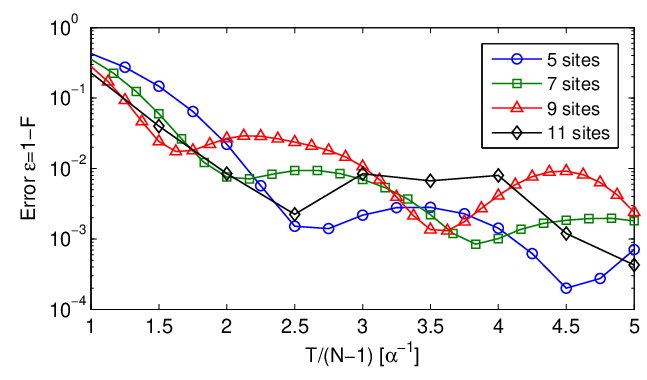
The error of the transfer process is given by $\epsilon=1-F$, with $F={}_{N}\langle 1|\rho_{N}(T)|1\rangle_{N}$ being the transfer fidelity. In Fig. 3, the error $\epsilon$ is plotted for different durations of the process and for chains of various lengths. Clearly, $\epsilon$ decreases as the transfer process is made slower. The maximal velocity $T/(N-1)$ permitted for state transfer with fixed maximal error decreases as $N$ is increased.

For the Hamiltonian considered here, the decrease of the transfer velocity as the number of sites is increased cannot be avoided, since the gap to the first excited state closes for $N\rightarrow\infty$. For small chains ($N\leq 11$) we have performed an exact diagonalization of $\hat{H}_{\rm bb}(x)$ to obtain $c(x)$ and $\Delta(x)$. Figs. 4 (a,b) show typical values of $c(x)$ and $\Delta(x)$ for the coupling of the ground state to the first excited state (both with the same total spin). The gap $\Delta(x)$ decreases approximately linear for $|x|$ varying from $1$ to $0$, while $c(x)$ is well described by a Lorentzian function. Clearly, both are sharply peaked at $x=0$. This suggest to use optimal control techniques to increase the (mean) transfer velocity by adapting the change of the spin-spin couplings, i.e., $dx(t)/dt$, to the instantaneous energy difference $\Delta(x)$ and the coupling $c(x)$.

In [22], a method has been developed to obtain an optimized path $x=x_{\rm opt}(t)$ which allows to suppress excitations to other states, i.e., to reduce the transition probability

To this aim, we replace $\int_{t^{\prime}=0}^{t}dt^{\prime}\Delta(x^{\prime}(t))=\frac{T}{T_{0}}\tau(t)$ (where $T_{0}$ is chosen to have $\tau(0)=0$ and $\tau(T)=1$), such that the integral becomes the Fourier transform of a function $u(\tau)\equiv\frac{dx(\tau)}{d\tau}c(x(\tau))$. Now, for $u(\tau)$ we choose a Blackman pulse [23] to reduce the side lobes of the Fourier transform. The shape $x(t)$ is then obtained from solving two differential equations in order to obtain first $x(\tau)$ (from inverting the equation for $u(\tau)$) and subsequently $\tau(t)$.

An example of a path $x(t)$ obtained in such a way is plotted in Fig. 4 (c). The dependence of the transfer error on the mean velocity $T/(N-1)$ if such an optimized path is used, is plotted in Fig. 5. Compared to the results for a linear change of $x$ in time, displayed in Fig. 3, the error for a given mean velocity is typically more than one magnitude smaller for the optimized path.

Let us finally discuss the implementation of the bilinear–biquadratic Heisenberg Hamiltonian and the realization of the spatial–temporal control of the couplings. We consider atoms with spin $F=1$ (i.e., atoms with an $2F+1$-dimensional hyperfine degree of freedom) at low temperatures confined in a deep (1D) optical lattice. The system then is well described via the Bose-Hubbard Hamiltonian [13, 26]

Here $\hat{a}_{i,\sigma}$ annihilates a particle in a hyperfine state with $m_{F}=\sigma$ at site $i$, $\hat{n}_{i}=\sum_{\sigma}\hat{a}_{i,\sigma}^{\dagger}\hat{a}_{i,\sigma}$ is the number of particles, and $\hat{\mbox{\boldmath$F$}}_{i}=\sum_{\sigma\sigma^{\prime}}\hat{a}^{\dagger}_{i,\sigma}\hat{\mbox{\boldmath$T$}}_{\sigma\sigma^{\prime}}\hat{a}_{i,\sigma^{\prime}}$ is the (total) spin operator on site $i$ ($\hat{\mbox{\boldmath$T$}}$ being the usual spin-$1$ matrices). The tunneling amplitude $t$ is obtained from the overlap of the Wannier functions $w(x)$ [26]. Tunneling conserves both, the total spin $S$ and the total spin projection $m_{S}$. The parameters $c_{0}=(g_{0}+2g_{2})/3$ and $c_{2}=(g_{2}-g_{0})/3$ depend on the effective 1D interaction strengths in the spin $S$ channel, $g_{S}$. Those are proportional to the two-body spin-dependent scattering length $a_{S}$. Their absolute strength can be controlled via the orthogonal confinement, the relative strength moreover can be changed via (magnetic or optical) Feshbach resonances. Note that due to the bosonic character of the particles, on-site contact interactions are zero for odd total spin.

The ratios $t/c_{0},\,t/c_{2}$ between tunneling and on-site interactions are tunable via the lattice parameters (lattice depth and orthogonal confinement). For $t\ll|c_{0}|,\,|c_{2}|$ the system is in a Mott-insulating state with atoms being quenched at fixed lattice sites. Here we will only consider the case of having a single particle per lattice site [15], and assume tunneling to be sufficiently weak compared to on-site interactions, such that it can be treated perturbatively with $t/c_{0}$ as small parameter. Then, the following effective spin-spin Hamiltonian can be obtained in second order perturbation theory [13]:

where $\tilde{c}_{2}=c_{2}/c_{0}$. This Hamiltonian is equivalent to the one of Eq. (1). For ²³Na, the bare values of the scattering lengths are very similar: $a_{0}=46a_{B},\,a_{2}=52a_{B}$ [27]. Then $\tilde{c}_{2}\approx 0.04$ and $\theta\approx-0.74\pi$. However, through auxiliary magnetic and electric fields, it is possible to modify the system such that the complete anti-ferromagnetic part of the phase diagram can be reached [14].

Let us now move to the realization of the adiabatic passage. The necessary spatial-temporal variation of the couplings can be realized by two pairs of laser beams of wavelengths $\lambda$ and $\lambda/2$, respectively, and identical polarizations, counter-propagating in $x$ direction (additional optical potentials in $y$- and $z$-direction are necessary to confine the atoms in 3D). The trapping potential in $x$-direction seen by the atoms then is proportional to the square of the electric field. Thus

where $I_{\rm half}$ and $I_{\rm full}$ are the corresponding laser intensities. We have introduced an additional phase shift $\phi_{\rm full}$ for the laser of wavelength $\lambda$. The effective spin-spin-coupling is proportional to $t^{2}$, see Eq. (20), which in turn has an exponential dependence on the height of the potential between adjacent sites. Setting only $I_{\rm half}>0$ (and $I_{\rm full}=0$), a lattice (with a distance of $\lambda/4$ between adjacent sites) is defined with all couplings being equal. We assume this lattice to be loaded with a single particle per site in the ground state. Setting $\phi_{\rm full}=\pi/2$, then $I_{\rm full}$ is increased to strongly reduce the coupling between each second pair of sites. At the same time, $I_{\rm half}$ has to be adjusted to keep the tunneling between the other sites in a regime where the effective Hamiltonian (20) is valid. This provides the initial situation for the transport process, c.f., Fig. 6 (a). After preparation of the first spin, $I_{\rm full}$ is decreased to zero (adjusting properly also $I_{\rm half}$; see Fig. 6 (b)), and $\phi_{\rm full}$ is set to zero. Then increasing $I_{\rm full}$ again allows to turn off selectively only the other subset of spin-spin-couplings [Fig. 6 (c)]. This procedure realizes the change of the Hamiltonian necessary for the adiabatic passage transfer process.

Finally, we can make a rough estimation of the time scales of the process which can be achieved with realistic optical lattice parameters. For ²³Na, $\lambda/2=514\,$nm, and for tight orthogonal confinement, in the perturbative regime ($|t/c_{0}|\ll 1$) couplings $\alpha=\hbar J$ with $J\approx 100\ldots 200\,$s^-1 could be achieved, leading to $T_{N=9}\approx(1\ldots 25)\cdot 10^{-2}\,$s for $N=9$ sites and an error $\epsilon<10^{-2}$ in the optimized case. For atoms with spin $F=1$, like Sodium, deep in the Mott insulating phase, decoherence is caused either by 3-body losses or by scattering of photons. Notice, however, that 3-body losses are relevant only for filling factors larger than two. If the lasers forming the optical lattice are far detuned from all atomic resonances, the spontaneous scattering rate is highly suppressed and coherence times much larger than $T_{N=9}$ are easily accessible. That means that the transport scheme we propose via adiabatic passage in spin chains should be experimentally realizable.

In this article we have presented a scheme to transfer a quantum state through a spin chain using an adiabatic passage technique. The most remarkable features of this scheme are the following. First, the transfer fidelity can be made arbitrarily close to one by increasing the transfer time. Second, as long as the change of the couplings is adiabatic, the transport fidelity does not depend on the exact path $x(t)$ in parameter space. There is thus no need of a precise control of couplings and timing. Third, in contrast to other transfer schemes in spin chains, there is no need for a receiver, meaning that once the transfer has been accomplished the system remains frozen.

We have applied this method to a spin-$1$ chain in the anti-ferromagnetic dimerized phase. Using standard optimal control techniques, we have shown that the transfer velocity can be substantially increased if an optimized path in parameter space is chosen. We have proposed a realistic experimental implementation of adiabatic passage transfer using ultracold atoms and optical superlattices.

In the spin-$1$ dimerized phase, the transfer velocity is limited by the fact that for a chain with an odd number of sites the gap vanishes as $N\rightarrow\infty$. Identifying a system with similar characteristics but with a gap that persists in the thermodynamic limit would allow for finite transfer velocities regardless the size of the chain.

We thank Diego Porras for enlightening discussions. We acknowledge support from MEC (Spanish Government) under contracts AP2005-0595, FIS 2005-04627, -014697, -01369, EX2005-0830, CIRIT SGR-00185, CONSOLIDER-INGENIO2010 CSD2006-00019 “QOIT”.

References

- [1] C.H. Bennett and D.P. DiVincenzo. Quantum information and computation. Nature 404, 247 (March 2000).
- [2] S. Bose. Quantum Communication through an Unmodulated Spin Chain. Phys. Rev. Lett. 91, 207901 (2003).
- [3] V. Subrahmanyam. Entanglement dynamics and quantum-state transport in spin chains. Phys. Rev. A 69, 034304 (2004).
- [4] M. Christandl, N. Datta, A. Ekert, and A.J. Landahl. Perfect State Transfer in Quantum Spin Networks. Phys. Rev. Lett. 92, 187902 (2004).
- [5] Y. Li, T. Shi, B. Chen, Z. Song, and C.-P. Sun. Quantum-state transmission via a spin ladder as a robust data bus. Phys. Rev. A 71, 022301 (2005).
- [6] A. Wojcik, T. Luczak, P. Kurzynski, A. Grudka, T. Gdala, and M. Bednarska. Unmodulated spin chains as universal quantum wires. Phys. Rev. A 72, 034303 (2005).
- [7] T.J. Osborne and N. Linden. Propagation of quantum information through a spin system. Phys. Rev. A 69, 052315 (2004).
- [8] H.L. Haselgrove, Optimal state encoding for quantum walks and quantum communication over spin systems. Phys. Rev. A 72 062326 (2005).
- [9] D. Burgarth and S. Bose. Conclusive and arbitrarily perfect quantum-state transfer using parallel spin-chain channels. Phys. Rev. A 71, 052315 (2005).
- [10] M.B. Plenio, J. Hartley, and J. Eisert. Dynamics and manipulation of entanglement in coupled harmonic systems with many degrees of freedom. New J. Phys. 6, 36 (2004).
- [11] M.B. Plenio and F.L. Semião. High efficiency transfer of quantum information and multiparticle entanglement generation in translation-invariant quantum chains. New J. Phys. 7, 73 (2005).
- [12] K. Buchta, G. Fáth, Ö. Legeza, and J. Sólyom Probable absence of a quadrupolar spin-nematic phase in the bilinear-biquadratic spin-1 chain. Phys. Rev. B 72, 054433 (2005).
- [13] A. Imambekov, M. Lukin, and E. Demler. Spin-exchange interaction of spin-one bosons in optical lattices: singlet, nematic, and dimerized phases. Phys. Rev. A 68, 063602 (2003).
- [14] J.J. García-Ripoll, M.A. Martin-Delgado, and J.I. Cirac. Implementation of Spin Hamiltonians in Optical Lattices. Phys. Rev. Lett. 93, 250405 (2004).
- [15] M. Rizzi, D. Rossini, G. De Chiara, S. Montangero, and R. Fazio. Phase Diagram of Spin-1 Bosons on One-Dimensional Optical Lattices. Phys. Rev. Lett. 95, 240404 (2005).
- [16] O. Romero-Isart, K. Eckert, and A. Sanpera. Quantum State Transfer in Spin-1 Chains: Uncovering the Magnetic Order. quant-ph/0610210.
- [17] I. Affleck, T. Kennedy, E.H. Lieb, and H. Tasaki. Valence bond ground states in Isotropic Quantum Antiferromagnets. Comm. Math. Phys. 115, 477 (1988).
- [18] S.K. Yip. Dimer State of Spin-1 Bosons in an Optical Lattice. Phys. Rev. Lett. 90, 250402 (2003).
- [19] A. Laeuchli, G. Schmid, and S. Trebst. Spin nematic correlations in bilinear-biquadratic S=1 spin chains. cond-mat/0607173.
- [20] L.I. Schiff. Quantum Mechanics. New York 1968.
- [21] S. Guérin, S. Thomas, and H. R. Jauslin. Optimization of population transfer by adiabatic passage. Phys. Rev. A 65, 023409 (2002).
- [22] W. Hänsel, J. Reichel, P. Hommelhoff, and T. W. Hänsch. Trapped-atom interferometer in a magnetic microtrap. Phys. Rev. A 64, 063607 (2001).
- [23] E. Harris The use of windows for harmonic analysis with the discrete Fourier transform. Proc. IEEE 66, 51 (1978).
- [24] G. Albertini. Is the purely biquadratic spin 1 chain always massive? cond-mat/0012439.
- [25] J.J Garcia-Ripoll. Time evolution algorithms for Matrix Product States and DMRG. New J. Physics 8, 305 (2006).
- [26] M. Lewenstein, A.Sanpera, V. Ahufinger, B. Damski, A. Sen De, and U. Sen. Ultracold atomic gases in optical lattices: Mimicking condensed matter physics and beyond. cond-mat/0606771.
- [27] J.P. Burke Jr., C.H. Greene, and J.L. Bohn. Multichannel Cold Collisions: Simple Dependences on Energy and Magnetic Field. Phys. Rev. Lett. 81, 3355 (1998).
- [28] A. Widera, F. Gerbier, S. Fölling, T. Gericke, O Mandel and I. Bloch, Coherent Collisional Dynamics in Optical Lattices. Phys. Rev. Lett. 95, 190405 (2005).
- [29] T. Ohshima, A. Ekert, D.K.L. Oi, D. Kaslizowski, and L.C. Kwek. Robust state transfer and rotation through a spin chain via dark passage. quant-ph/0702019.