Dipartimento di Fisica “E. R. Caianiello”
Facoltà di Scienze Matematiche Fisiche e Naturali
Dr. Fabrizio Illuminati
\HUGEENTANGLEMENT OF
GAUSSIAN
STATES
Coordinator: Prof. G. Vilasi
Abstract
This Dissertation collects results of my own work on the interpretation, characterization, quantification and application of bipartite and multipartite entanglement in Gaussian states of continuous variable (CV) systems.11 1 Most of the research achievements presented here are published in (or under consideration for) scientific papers, as listed on page 15.B.1. My publications will be quoted as [GAx] throughout the Dissertation. Some results, excluding the most recent advances, are also summarized in a book chapter [GA22]. The structural and theoretical parts of this Dissertation are the basis for a review article [GA23].
In the context of investigating connections between bipartite entanglement and global and local degrees of information [GA1, GA6], we show how entanglement of two-mode Gaussian states can be accurately quantified in terms of the global and local amounts of mixedness [GA2, GA3], and efficiently estimated experimentally by direct measurements of the associated purities [GA2, GA8]. More generally, we discuss different measures of bipartite entanglement and show their inequivalence in ordering two-mode Gaussian states [GA7]. For multimode Gaussian states endowed with local symmetry with respect to a given bipartition, we show how the multimode block entanglement can be completely and reversibly localized onto a single pair of modes by local, unitary operations [GA4, GA5].
We then analyze the distribution of entanglement among multiple parties in multimode Gaussian states [GA12], introducing a new entanglement monotone, the ‘contangle’, adapted to a CV scenario [GA10]. We prove that, in all Gaussian states of an arbitrary number of modes, entanglement distributes (as already observed for qubit systems) according to a monogamy law [GA10, GA15]. Focusing on three-mode Gaussian states, we study their genuine tripartite entanglement by means of the residual contangle [GA10], we discuss their usefulness for quantum communication implementations [GA16], and we investigate in detail their distributed entanglement structure [GA11], evidencing how, under a strong symmetry, an arbitrary tripartite entanglement coexists with a limited, nonzero bipartite entanglement: a feature named ‘promiscuous’ entanglement sharing [GA10]. We then unfold how in four-mode Gaussian states with more relaxed symmetry constraints, entanglement can be infinitely promiscuous (at variance with the corresponding states of qubits), with a coexistence of an unlimited four-partite entanglement and an unlimited residual bipartite entanglement in two pairs of modes [GA19].
We moreover study entanglement distribution in harmonic lattices with an underlying ‘valence bond’ structure [GA13, GA17], and, in the general case of pure N-mode Gaussian states, we provide standard forms under local operations [GA18], which yield an efficient characterization of generic entanglement, together with an optimal scheme to engineer such states in the lab with minimal resources [GA14]. Operationally, multipartite entanglement in symmetric N-mode Gaussian resources is qualitatively and quantitatively proven to be equivalent to the success of multiparty CV quantum teleportation networks [GA9]. We conclude with an application of our machinery to a relativistic setting: namely, we study Gaussian entanglement sharing between modes of a free scalar field from the perspective of observers in relative acceleration, interpreting the entanglement loss due to the Unruh effect in the light of a redistribution of entanglement between accessible and unaccessible causally disconnected modes [GA20]. Such studies are of relevance in the context of the information loss paradox in black holes [GA21].
![[Uncaptioned image]](0702069v1/dedica.png)
![[Uncaptioned image]](0702069v1/lifesentanglement.png)
Life’s Entanglement. CR
Studio Inc., 2002.
http://www.crstudioinc.com/paint/54.html
Foreword
Three years have passed quickly but at the same time filled with entertainment, work and new experiences which have left an indelible footprint on my formation. I have shared this adventure with many people, and it is a pity I cannot list them all here for brevity reasons.
Many thanks with sincere appreciation and esteem to my advisor Dr. Fabrizio Illuminati for all the simultaneously funny and serious time, for having taught me how to make top-quality research and how to write papers in a unique style. We had many animated discussions, and he was always prompt to give me wise advices without ever imposing his point of view, or preventing me to take my own decisions. Thanks also for his breathtaking attributes when referring to me in letters of support. I am grateful to Prof. Silvio De Siena, who leads with Fabrizio the Quantum Theory and Quantum Technologies Group in Salerno: his patience, experience and friendliness have been useful in several critical moments. It is impossible not to smile while thinking of, and thanking my friend and colleague Dr. Alessio Serafini (now at Imperial College, London), arguably the only person with whom I was able to establish a ‘proper’ collaboration (and who managed to have me doing calculations with pencil and paper): he is to be blamed for introducing me to continuous variable systems and Gaussian states. I hope to keep sharing ideas with him, even though the shiny “basset-crew” trio (me, him and Fabrizio) is now spatially separated.
During my PhD I had the luck of spending one year in the Centre for Quantum Computation (CQC) of the University of Cambridge. I cannot recall how many interesting discussions (mostly at lunch-time) arose there, and an estimate of how much the Cambridge experience was good for myself (on both professional and personal grounds) would surely result in a lower bound. Hence I express all my gratitude to my host Dr. Marie Ericsson for the joy of making physics together, for her enthusiastic attitude towards work, and for the friendship born during my year at CQC. Accordingly, I thank Prof. Artur Ekert, director of the CQC, who accepted me as a full member, and whose (quantum) capacity of efficiently transmitting advices in short-time interactions is probably close to infinity.
I acknowledge collaborating with several researchers during these years. First, thanks to the experimental group of Prof. Claude Fabre (Lab. Kastler-Brossel, Paris), and specifically to Dr. Julien Laurat (now at Caltech), Dr. Thomas Coudreau, Gaëlle Keller and José Augusto Oliveira-Huguenin, for the fruitful exchanges and for letting me see what a beam-splitter is in reality. Thanks also to Tohya Hiroshima for welcoming our contribution to the proof of the monogamy of entanglement in all Gaussian states, and to Ivette Fuentes-Schuller for the relativistic insights coming from our joint project on continuous variable entanglement in non-inertial reference frames. I am furthermore deeply grateful to a series of colleagues, not enumerated here, whom I met in various venues and with whom I discussed for brief or long time, learning new things and understanding old ones.
Thanks to Alfonso and to all my friends, colleagues and officemates both in Salerno and in Cambridge: time without them would have been duller and less productive. Thanks to my parents, my sister and all close members of my family, for their neverending encouragement and for the trust they placed in me. Special thanks to www.enigmi.net for keeping my brain active during this last year.
My unlimited thanks and love to Samanta, whom I had the pleasure and honor to marry in the middle of our PhD. Thanks for all her support, hints, criticisms, proofreading, thanks for reminding me of the sentence quoted in the caption of Fig. 12, thanks for all her delicious dinners, her sweetness, her patience, her kisses, her love, for all her being herself. Thanks for making a better man out of me… and for the miracle of life which blessed her and me.
Gerardo
Part I Preliminaries
![[Uncaptioned image]](0702069v1/briansguide.png)
Brian’s guide to quantum
mechanics. John Walker, 2006.
http://www.briansguide.net/index.cgi?ID=1140392885-C-CSI
Introduction
About eighty years after their inception, quantum mechanics and quantum theory are still an endless source of new and precious knowledge on the physical world and at the same time keep evolving in their mathematical structures, conceptual foundations, and intellectual and cultural implications. This is one of the reasons why quantum physics is still so specially fascinating to all those that approach it for the first time and never ceases to be so for those that are professionally involved with it. In particular, since the early nineties of the last century and in the last ten-fifteen years, a quiet revolution has taken place in the quantum arena. This revolution has progressively indicated and clarified that aspects once thought to be problematic, such as quantum non-separability and “spooky” actions at a distance, are actually not only the origin of paradoxes but rather some of the key ingredients that are allowing a deeper understanding of quantum mechanics, its applications to new and exciting fields of research (such as quantum information and quantum computation), and tremendous progress in the development of its mathematical and conceptual foundations. Among the key elements of the current re-foundation of quantum theory, entanglement certainly plays a very important role, also because it is a concept that can be mathematically qualified and quantified in a way that allows it to provide new and general characterizations of quantum properties, operations, and states.
The existence of entangled states, stemming directly from the superposition principle, can be regarded as a founding feature, or better “the characteristic trait” (according to Schrödinger) of quantum mechanics itself. Entanglement arises when the state of two or more subsystems of a compound quantum system cannot be factorized into pure local states of the subsystems. The subsystems thus share quantum correlations which can be stronger than any classical correlation. Quantum information science was born upon the key observation that the exploitation of such nonclassical correlations enables encoding, processing and distribution of information in ways impossible, or very inefficient, with classical means. Hence the possibility of implementing entangled resources resulted in futuristic proposals (quantum teleportation, quantum cryptography, quantum computation, …) which are now made, to a certain extent, into reality. On a broader perspective, it is now recognized that entanglement plays a fundamental role in the physics of many-body systems, in particular in critical phenomena like quantum phase transitions, and in the description of the interactions between complex systems at the quantum scale.
Despite its prominent role in the physics of microscopic but also macroscopic systems, it still stands as an open issue to achieve a conclusive characterization and quantification of bipartite entanglement for mixed states, and especially to provide a definition and interpretation of multipartite entanglement both for pure states and in the presence of mixedness. While important insights have been gained on these issues in the context of qubit systems (two-level quantum systems traditionally employed as the main logical units for quantum computing and quantum information in general), a less satisfactory understanding has been achieved until recent times on higher-dimensional systems, as the structure of entangled states in Hilbert spaces of high dimensionality scales exhibiting a formidable degree of complexity.
However, and quite remarkably, in systems endowed with infinite-dimensional Hilbert spaces (where entanglement can arise between degrees of freedom with continuous spectra), recent advances have been recorded for what concerns the understanding and the quantification of the entanglement properties of a restricted class of states, the so-called Gaussian states. Gaussian states distinctively stand out of the infinite variety of continuous variable systems, because on one hand they allow a clean framework for the analytical study of the structure of non-local correlations, and on the other hand they are of great practical relevance in applications to quantum optics and quantum information. Two-mode and multimode coherent and squeezed Gaussian states are indeed key resources, producible and manipulatable in the lab with a high degree of control, for a plethora of two-party and multi-party quantum communication protocols, ranging from deterministic teleportation and secure key distribution, to quantum data storage and cluster computation.
This PhD Dissertation collects my personal contributions to the understanding, qualification, quantification, structure, production, operational interpretation, and applications of entanglement in Gaussian states of continuous variable systems. Let us briefly mention some of the most important results, the majority of which have appeared in Refs. [GA2—GA20].
In the first place we enriched the well-established theory of bipartite entanglement in two-mode Gaussian states, providing new physically insightful connections between the entanglement and the degrees of information associated with the global system and its subsystems. We thus showed that the negativity (an entanglement monotone) can be accurately qualified and quantitatively estimated in those states by direct purity measurements. We also proved that different entanglement quantifiers (negativities and Gaussian entanglement measures) induce inequivalent orderings on the set of entangled, nonsymmetric two-mode Gaussian states. We then extended our scope to investigate multimode, bipartite entanglement in -mode Gaussian states endowed with some symmetry constraints, and its scaling with the number of the modes; this study was enabled by our central observation that entanglement in such states is unitarily localizable to an effective two-mode entanglement. We could thus extend the validity of the necessary and sufficient positive-partial-transposition condition for separability to bisymmetric Gaussian states of an arbitrary number of modes, and exactly quantify the block entanglement between different mode partitions, revealing signatures of a genuine multipartite entanglement arising among all modes. Under these premises, we developed ex novo a theory of multipartite entanglement for Gaussian states, based on the crucial fact that entanglement cannot be freely shared and its distribution is constrained to a monogamy inequality, which we proved to hold for all (pure and mixed) -mode Gaussian states distributed among parties. To this aim, we introduced new continuous variable entanglement monotones, namely (Gaussian) ‘contangle’ and Gaussian tangle, for the quantification of entanglement sharing in Gaussian states. Implications of this analysis include, in particular, the definition of the ‘residual contangle’ as the first bona fide measure of genuine multipartite (specifically, tripartite) entanglement in a continuous variable setting, a complete quantitative analysis of multipartite entanglement in the paradigmatic instance of three-mode Gaussian states, the discovery of the promiscuous nature of entanglement sharing in symmetric ‘GHZ/’ Gaussian states, and the demonstration of the possible coexistence of unlimited bipartite and multipartite entanglement in states of at least four modes.
Our investigation was not confined to theoretical and structural aspects of entanglement only. Along parallel lines, we got interested on one hand in how to produce bipartite and/or multipartite entanglement in the lab with efficient means, and on the other hand in how to optimally employ such entanglement for practical applications, endowing the entanglement itself with an operational interpretation. In the case of two-mode Gaussian states, we joined an experiment concerning production, characterization and manipulation of entanglement in the context of quantum optics. In the three- and four-mode instances, we proposed several schemes to efficiently engineer family of Gaussian states with relevant entanglement properties. In general, we devised an optimal scheme to produce generic pure -mode Gaussian states in a standard form not encoding direct correlations between position and momentum operators (and so encompassing all the instances of multimode Gaussian states commonly employed in practical implementations); such an analysis allows to interpret entanglement in this subclass of Gaussian states entirely in terms of the two-point correlations between any pair of modes. In this respect, one theoretical result of direct interest for the characterization of entanglement in Gaussian states, is the qualitative and quantitative equivalence we established between the presence of bipartite (multipartite) entanglement in two-mode (-mode) fully symmetric Gaussian states shared as resources for a two-party teleportation experiment (-party teleportation network), and the maximal fidelity of the protocol, optimized over local single-mode unitary operations performed on the shared resource. In the special case of three-mode, pure GHZ/ states, this optimal fidelity is a monotonically increasing function of the residual contangle (which quantifies genuine tripartite entanglement), providing the latter with a strong operational significance. Based on this equivalence, we presented a proposal to experimentally verify the promiscuous sharing structure of tripartite Gaussian entanglement in such states in terms of the success of two-party and three-party teleportation experiments. Telecloning with three-mode Gaussian resources was also thoroughly investigated.
We finally considered two applications of the Gaussian machinery to the companion areas of condensed matter/statistical mechanics, and relativity theory. Concerning the former, we studied entanglement distribution in ground states of translationally invariant many-body harmonic lattice systems endowed with a Gaussian ‘valence bond’ structure. We characterized the range of correlations in such harmonic models, connecting it to the degree of entanglement in a smaller Gaussian structure, named ‘building block’, which enters in the valence bond construction. We also discussed the experimental production of Gaussian valence bond states of an arbitrary number of modes, and their usefulness for multiparty telecloning of coherent states. On the other hand, in a relativistic setting we studied the distribution of entanglement between modes of a free scalar field from the perspective of observers in relative acceleration. The degradation of entanglement due to the Unruh effect was analytically characterized for two parties sharing a two-mode Gaussian state in an inertial frame, in the cases of either one or both observers undergoing uniform acceleration. Within the monogamy framework, we precisely explained the loss of entanglement as a redistribution of the inertial entanglement into multipartite quantum correlations among accessible and unaccessible modes from a non-inertial perspective.
This Dissertation is organized as follows.
Part I is devoted to introducing the main ingredients of our analysis, entanglement on one side, and Gaussian states on the other. In particular, Chapter 1 contains the basics of entanglement theory: how to quantify quantum information, the separability problem, different entanglement measures, and a discussion on entanglement sharing. In Chapter 2 we give a self-contained introduction to phase-space and symplectic methods in the study of Gaussian states of infinite-dimensional bosonic systems, we discuss the covariance matrix formalism, and we provide a classification of pure and mixed Gaussian states according to the various standard forms that the associated covariance matrices can take.
We collect in Part II all results concerning bipartite entanglement of Gaussian states with two or more modes. In Chapter 3 we illustrate the machinery of bipartite entanglement qualification and quantification in Gaussian states. The massive Chapter 4 contains our specific results on two-mode Gaussian states, including the existence of extremally (minimally and maximally) entangled states at given degrees of mixedness, and the different orderings induced on entangled states by different measures of entanglement. In Chapter 5 we describe the unitary (and therefore reversible) localization of bipartite multimode entanglement to a bipartite two-mode entanglement in fully symmetric and bisymmetric multimode Gaussian states, and its scaling with the number of modes.
Multipartite entanglement of Gaussian states is the topic of Part III. In Chapter 6 we present our crucial advances in the understanding of entanglement sharing in multimode Gaussian states, including the proof of the monogamy inequality on distributed entanglement for all Gaussian states. Multipartite entanglement of three-mode Gaussian states is analyzed in Chapter 7 by discussing the structural properties of such states, and the main consequences of the monogamy inequality, such as the quantification of genuine tripartite entanglement, and the promiscuous nature of entanglement sharing in Gaussian states with symmetry properties. Chapter 8 deals with the remarkable property of multipartite entanglement in Gaussian states (as opposed to low-dimensional systems), to coexist to an arbitrary extent with bipartite entanglement, in simple families of states of at least four modes, within the holding of the monogamy inequality.
In Part IV we show how to engineer multimode Gaussian resources with optical means. Chapter 9 contains schemes for the production of extremally entangled two-mode states, as well as experimental results on the production, characterization and manipulation of two-mode entanglement with a novel optical setup. In Chapter 10 we provide a systematic investigation on the preparation of several families of three- and four-mode Gaussian states with peculiar entanglement properties, providing efficient schemes. Chapter 11 deals instead with the general instance of pure -mode Gaussian states, in which case for the relevant family of ‘block-diagonal’ states an optimal state engineering recipe is proposed, which enables to connect generic entanglement to operationally meaningful resources.
The companion Part V looks at entanglement from a practical perspective for quantum information and communication implementations, and other less conventional applications. Bipartite and multipartite teleportation-based communication (including telecloning) with Gaussian states is studied in Chapter 12, where the equivalence between optimal teleportation fidelity and shared entanglement is established, together with an experimentally testable connection between teleportation efficiency, multipartite entanglement, and promiscuous sharing structure. Entanglement distribution and the investigation of the correlation range in many-body harmonic rings with a Gaussian valence bond structure is addressed in Chapter 13. The degradation of Gaussian entanglement as detected by accelerated observers is instead investigated in Chapter 14, and interpreted in terms of an entanglement re-distribution in multipartite form among accessible and unaccessible modes from a non-inertial perspective.
Part VI concludes this Dissertation with a summary on the various applications of Gaussian entanglement not covered by our personal research, a brief discussion about recent advances in the qualification and quantification of entanglement in non-Gaussian states — a field of investigation that is to a large extent yet to be fully explored — and an overview on open problems and current research directions. Appendix 15 contains some tools of symplectic analysis necessary for the structural characterization of the covariance matrix of pure Gaussian states.
Chapter 1 Characterizing entanglement
According to Erwin Schrödinger, quantum entanglement is not “one but rather the characteristic trait of quantum mechanics, the one that enforces its entire departure from classical lines of thought” [201]. Entanglement has been widely recognized as a fundamental aspect of quantum theory, stemming directly from the superposition principle and quantum non-factorizability. Remarkably, it is now also acknowledged as a fundamental physical resource, much on the same status as energy and entropy, and as a key factor in the realization of information processes otherwise impossible to implement on classical systems. Thus the degree of entanglement and information are the crucial features of a quantum state from the point of view of Quantum Information Theory [163, 111]. Indeed, the search for proper mathematical frameworks to quantify such features in general (mixed) quantum states cannot be yet considered accomplished. In view of such considerations, it is clear that the full understanding of the relationships between the quantum correlations contained in a multipartite state and the global and local (i.e. referring to the reduced states of the subsystems) degrees of information of the state, is of critical importance. In particular, it would represent a relevant step towards the clarification of the nature of quantum correlations and, possibly, of the distinction between quantum and classical correlations in mixed quantum states [112, 13, 101].
We open this Chapter with a discussion about the interpretation and measures of information in quantum systems. We then move to a detailed discussion about quantum entanglement, its definition, qualification and quantification in the bipartite and, to some extent, in the multipartite setting. Special attention will be devoted to the fundamental property of entanglement to be distributed in a so-called “monogamous” way, and the implications of such feature for the characterization of many-body entanglement sharing.
1 Information contained in a quantum state
Both discrete-variable and continuous-variable systems, endowed respectively with a finite-dimensional and a infinite-dimensional Hilbert space, can be efficiently employed in quantum information theory for the encoding, manipulation and transmission of information. In this context, it is natural to question how much information a quantum state contains.
Suppose we have prepared a physical system in a certain state and we would like to test the system somehow, for instance with a measurement. Before performing the experimental verification, we can only predict the probabilities associated to the possible outcomes. After the measurement, one of these outcomes will have occurred and we will possess a complete information (certainty) about the state of our system.
The degree of information contained in a state corresponds to how much certainty we possess a priori on predicting the outcome of any test performed on the state [177].
1.1 Purity and linear entropy
The quantification of information will in general depend not only on the state preparation procedure, but also on the choice of the measurement with its associated probabilities . If for any test one has a complete ignorance (uncertainty), i.e. for a system in a -dimensional Hilbert space one finds , then the state is maximally mixed, in other words prepared in a totally random mixture, with density matrix proportional to the identity, . For instance, a photon emitted by a thermal source is called ‘unpolarized’, reflecting the fact that, with respect to any unbiased polarization measurement, the two outcomes (horizontal/vertical) have the same probability. The opposite case is represented by pure quantum states, whose density matrix is a projector , such that . A pure state of a quantum system contains the maximum information one has at disposal on the preparation of the system. All the intermediate instances correspond to a partial information encoded in the state of the system under consideration.
A hint on how to quantify this information comes from the general properties of a quantum density operator. We recall that
It is thus natural to address the trace of as purity of a state ,
| (1) |
The purity is a measure of information. For states of a Hilbert space with , the purity varies in the range
reaching its minimum on the totally random mixture, and equating unity of course on pure states. In the limit of continuous variable systems , the minimum purity tends asymptotically to zero.
Accordingly, the “impurity” or degree of mixedness of a quantum state , which characterizes our ignorance before performing any quantum test on , can be quantified via the functional
| (2) |
The quantity (ranging between and ) defined by Eq. (2) is known as linear entropy and it is a very useful measure of mixedness in quantum information theory due to its direct connection with the purity and the effective simplicity in its computation. Actually, the name ‘linear entropy’ follows from the observation that can be interpreted as a first-order approximation of the canonical measure of lack-of-information in quantum theory, that is Von Neumann entropy. In practice, the two quantities are not exactly equivalent, and differences between the two will be singled out in the context of characterizing entanglement, as we will see in the next Part.
1.2 Shannon–Von Neumann entropy
Let us go back to our physical system and to our ensemble of a priori known probabilities , associated to the possible outcomes of a particular measurement we are going to perform on the system. If we imagine to repeat the measurement on copies of the system, all prepared in the same state, with arbitrarily large, we can expect the outcome “system in state ” be obtained times. Based on our knowledge on the preparation of the system, we are in the position to predict the statistical frequencies corresponding to the different outcomes, but not the order in which the single outcomes will be obtained. Assuming that, on measurement runs, outcome is obtained times, outcome times, and so on, the total number of permutations of the outcomes is given by For , also the individual frequencies will diverge, , so that by using Stirling’s formula one finds
The expression
| (3) |
is named entropy associated to the probability distribution : it is a measure of our ignorance prior to the measurement.
The notion of entropy, originating from thermodynamics, has been reconsidered in the context of classical information theory by Shannon [213]. In quantum information theory the probabilities of Eq. (3) are simply the eigenvalues of the density matrix , and Shannon entropy is substituted by Von Neumann entropy [258]
| (4) |
Purity , linear entropy and Von Neumann entropy of a quantum state are all invariant quantities under unitary transformations, as they depend only on the eigenvalues of . Moreover, Von Neumann entropy satisfies a series of important mathematical properties, each reflecting a well-defined physical requirement [260]. Some of them are listed as follows.
- •
Concavity.
(5) with . Eq. (5) means that Von Neumann entropy increases by mixing states, i.e. is greater if we are more ignorant about the preparation of the system. This property follows from the concavity of the log function.
- •
Subadditivity. Consider a bipartite system (described by the Hilbert space ) in the state . Then
(6) where are the reduced density matrices associated to subsystems . For states of the form , Eq. (6) is saturated, yielding that Von Neumann entropy is additive on tensor product states:
(7) The purity, Eq. (1), is instead multiplicative on product states, as the trace of a product equates the product of the traces:
(8) - •
It is interesting to remark that Ineq. (6) is in sharp contrast with the analogous property of classical Shannon entropy,
| (11) |
Shannon entropy of a joint probability distribution is always greater than the Shannon entropy of each marginal probability distribution, meaning that there is more information in a global classical system than in any of its parts. On the other hand, consider a bipartite quantum system in a pure state . We have then for Von Neumann entropies: , while . The global state has been prepared in a well defined way, but if we measure local observables on the subsystems, the measurement outcomes are unavoidably random and to some extent unpredictable. We cannot reconstruct the whole information about how the global system was prepared in the state (apart from the trivial instance of being a product state ), by only looking separately at the two subsystems. Information is rather encoded in non-local and non-factorizable quantum correlations — entanglement — between the two subsystems. The comparison between the relations Eq. (6) and Eq. (11) clearly evidences the difference between classical and quantum information.
1.3 Generalized entropies
In general, the degree of mixedness of a quantum state can be characterized completely by the knowledge of all the associated Schatten –norms [18]
| (12) |
In particular, the case is directly related to the purity , Eq. (1), as it is essentially equivalent (up to normalization) to the linear entropy Eq. (2). The -norms are multiplicative on tensor product states and thus determine a family of non-extensive “generalized entropies” [17, 232], defined as
| (13) |
These quantities have been introduced independently Bastiaans in the context of quantum optics [17], and by Tsallis in the context of statistical mechanics [232]. In the quantum arena, they can be interpreted both as quantifiers of the degree of mixedness of a state by the amount of information it lacks, and as measures of the overall degree of coherence of the state.
The generalized entropies ’s range from for pure states to for completely mixed states with fully degenerate eigenspectra. We also mention that, in the asymptotic limit of arbitrary large , the function becomes a function only of the largest eigenvalue of : more and more information about the state is discarded in such an estimate for the degree of purity; considering for any non-pure state in the limit , yields a trivial constant null function, with no information at all about the state under exam. We also note that, for any given quantum state, is a monotonically decreasing function of .
1.4 Mutual information
The subadditivity property (6) of Von Neumann entropy is at the heart of the measure typically employed in quantum information theory to quantify total — classical and quantum — correlations in a quantum state, namely the mutual information [101]
| (16) |
where is the state of the global system and correspond to the reduced density matrices. Mutual information quantifies the information we obtain on by looking at the system in its entirety, minus the information we can extract from the separate observation of the subsystems. It can in fact be written as relative entropy between and the corresponding product state ,
| (17) |
where the relative entropy, a distance-like measure between two quantum states in terms of information, is defined as [243]
| (18) |
If is a pure quantum state [], the Von Neumann entropy of its reduced states quantifies the entanglement between the two parties, as we will soon show. Being in this case, one says that the pure state also contains some classical correlations, equal in content to the quantum part, .
In mixed states a more complex scenario emerges. The mere distinction between classical correlations, i.e. producible by means of local operations and classical communication (LOCC) only, and entanglement, due to a purely quantum interaction between subsystems, is a highly nontrivial, and not generally accomplished yet, task [112, 101].
We are now going to summarize the most relevant results to date concerning the qualitative and quantitative characterization of entanglement.
2 Entanglement and non-locality
From a phenomenological point of view, the phenomenon of entanglement is fairly simple. When two physical systems come to an interaction, some correlation of a quantum nature is generated between the two of them, which persists even when the interaction is switched off and the two systems are spatially separated22 2 Entanglement can be also created without direct interaction between the subsystems, via the so-called entanglement swapping [22].. If we measure a local observable on the first system, its state collapses of course in an eigenstate of that observable. Surprisingly, also the state of the second system, wherever it is (in the ideal case of zero environmental decoherence), is modified instantly. Responsible for this “spooky action at a distance” [73] is the non-classical and non-local quantum correlation known as entanglement.
Suppose we have a bipartite or multipartite quantum state: well, the answer to an apparently innocent question like
Does this state contain quantum correlations?
is extremely hard to be achieved [111, 13, 188]. The first step concerns a basic understanding of what such a question really means.
One may argue that a system contains quantum correlations if the observables associated to the different subsystems are correlated, and their correlations cannot be reproduced with purely classical means. This implies that some form of inseparability or non-factorizability is necessary to properly take into account those correlations. For what concerns globally pure states of the composite quantum system, it is relatively easy to check if the correlations are of genuine quantum nature. In particular, it is enough to check if a Bell-CHSH inequality [19, 58] is violated [96], to conclude that a pure quantum state is entangled. There are in fact many different criteria to characterize entanglement, but all of them are practically based on equivalent forms of non-locality in pure quantum states.
These equivalences fade when we deal with mixed states. At variance with a pure state, a mixture can be prepared in (generally infinitely) many different ways. Not being able to reconstruct the original preparation of the state, one cannot extract all the information it contains. Accordingly, there is not a completely general and practical criterion to decide whether correlations in a mixed quantum state are of classical or quantum nature. Moreover, different manifestations of quantum inseparability are in general not equivalent. For instance, one pays more (in units of Bell singlets) to create an entangled mixed state — entanglement cost [24] — than what one can get back from reconverting into a product of singlets — distillable entanglement [24] — via LOCC [276]. Another example is provided by Werner in a seminal work [264], where he introduced a parametric family of mixed states (known as Werner states) which, in some range of the parameters, are entangled (inseparable) without violating any Bell inequality on local realism, and thus admitting a description in terms of local hidden variables. It is indeed an open question in quantum information theory to prove whether any entangled state violates some Bell-type inequality [1, 229].
In fact, entanglement and non-locality are different resources [42]. This can be understood within the general framework of no-signalling theories which exhibit even more non-local features than quantum mechanics. Let us briefly recall what is intended by non-locality according to Bell [20]: there exists in Nature a channel that allows one to distribute correlations between distant observers, such that the correlations are not already established at the source, and the correlated random variables can be created in a configuration of space-like separation, i.e. no normal signal (assuming no superluminal transmission) can be the cause of the correlations [73, 19]. A convenient description of the intriguing phenomenon of non-locality is already known: quantum mechanics describes the channel as a pair of entangled particles. But such interpretation is not the only one. In recent years, there has been a growing interest in providing other descriptions of this channel, mainly assuming a form of communication [227], or the usage of an hypothetical “non-local machine” [189] able to violate the CHSH inequality [58] up to its algebraic value of (while the local realism threshold is and the maximal violation admitted by quantum mechanics is , the Cirel’son bound [57]). Usually, the motivation for looking into these descriptions does not come from a rejection of quantum mechanics and the desire to replace it with something else; rather the opposite: the goal is to quantify how powerful quantum mechanics is by comparing its achievements to those of other resources. The interested reader may have a further look at Ref. [98].
3 Theory of bipartite entanglement
3.1 Pure states: qualification and quantification
Definition 1
A pure quantum state is separable if it can be written as a product state, i.e. if there exist and such that
| (19) |
Otherwise, is an entangled state.
Qualifying entanglement means having an operational criterion which would allow us to answer our original question, namely if a given state is entangled or not.
To this aim, it is useful to write a pure quantum state in its unique Schmidt decomposition [191],
| (20) |
| (21) | |||||
| (22) |
The number of non-zero terms in the expansion (20) is known as Schmidt number, the positive numbers are the Schmidt coefficients, and the local bases and are the Schmidt bases.
From the Schmidt decomposition it follows that the reduced density matrices of ,
| (23) |
have the same nonzero eigenvalues (equal to the squared Schmidt coefficients) and their total number is the Schmidt number . One can then observe that product states are automatically written in Schmidt form with , i.e. the reduced density matrices correspond to pure states (. On the other hand, if a state admits a Schmidt decomposition with only one coefficient, then it is necessarily a product state. We can then formulate an entanglement criterion for pure quantum states. Namely, a state of a bipartite system is entangled if and only if the reduced density matrices describe mixed states,
| (24) |
with defined by Eq. (21).
We thus retrieve that bipartite entanglement of pure quantum states is qualitatively equivalent to the presence of local mixedness, as intuitively expected. This connection is in fact also quantitative. The entropy of entanglement of a pure bipartite state is defined as the Von Neumann entropy, Eq. (4), of its reduced density matrices [21],
| (25) |
The entropy of entanglement is the canonical measure of bipartite entanglement in pure states. It depends only on the Schmidt coefficients , not on the corresponding bases; as a consequence it is invariant under local unitary operations
| (26) |
It can be shown [190] that cannot increase under LOCC performed on the state : this is a fundamental physical requirement as it reflects the fact that entanglement cannot be created via LOCC only [245, 249]. It can be formalized as follows. Let us suppose, starting with a state of the global system , to perform local measurements on and , and to obtain, after the measurement, the state with probability , the state with probability , and so on. Then
| (27) |
Note that entanglement cannot increase on average, i.e. nothing prevents, for a given , that . On this the concept of entanglement distillation is based [23, 24, 97]: with a probability , it is possible to increase entanglement via LOCC manipulations.
3.2 Mixed states: entanglement vs separability
A mixed state can be decomposed as a convex combination of pure states,
| (28) |
Eq. (28) tells us how to create the state described by the density matrix : we have to prepare the state with probability , the state with probability , etc. For instance, we could collect copies () of the system, prepare of them in the state , and pick a random system.
The problem is that the decomposition of Eq. (28) is not unique: unless is already a pure state, there exist infinitely many decompositions of a generic in ensembles of pure states, meaning that the mixed state can be prepared in infinitely many different ways. One can expect that this has some consequence on the entanglement. Let us suppose we have a bipartite system and we detect, by local measurements, the presence of correlations between the two subsystems. Given the ambiguity on the state preparation, we cannot know a priori if those correlations arose from a quantum interaction between the subsystems (meaning entanglement) or were induced by means of LOCC (meaning classical correlations). It is thus clear that a mixed state can be defined separable (classically correlated) if there exist at least one way of engineering it by LOCC; on the other hand it is entangled (quantumly correlated) if, among the infinite possible preparation procedures, there is no one which relies on LOCC only [264].
Definition 2
A mixed quantum state of a bipartite system, described by the Hilbert space , is separable if and only if there exist coefficients , and states and , such that
| (29) |
Otherwise, is an entangled state.
For pure states, the expansion Eq. (29) has a single term and we recover Def. 1, i.e. the only separable pure states are product states. For mixed states, not only product states (containing zero correlations of any form) but in general any convex combination of product states is separable. This is obvious as the state of Eq. (29) contains only classical correlations, since it can be prepared by means of LOCC.
However, Def. 2 is in all respects impractical. Deciding separability according to the above definition would imply checking all the infinitely many decomposition of a state and looking for at least one of the form Eq. (29), to conclude that the state is not entangled. This is clearly impossible. For this reason, several operational criteria have been developed in order to detect entanglement in mixed quantum states [144, 43, 143]. Two of them are discussed in the following.
3.2.1 Positive Partial Transposition criterion
One of the most powerful results to date in the context of separability criteria is the Peres–Horodecki condition [178, 118]. It is based on the operation of partial transposition of the density matrix of a bipartite system, obtained by performing transposition with respect to the degrees of freedom of one subsystem only. Peres criterion states that, if a state is separable, then its partial transpose (with respect e.g. to subsystem ) is a valid density matrix, in particular positive semidefinite, The same holds naturally for . Positivity of the partial transpose (PPT) is therefore a necessary condition for separability [178]. The converse (i.e. separable) is in general false. The Horodecki’s have proven that it is indeed true for low-dimensional systems, specifically bipartite systems of dimensionality and , in which case PPT is equivalent to separability [118]. For higher dimensional systems, PPT entangled states (with ) have been shown to exist [122]. These states are known as bound entangled [119] as their entanglement cannot be distilled to obtain maximally entangled states. The existence of bound entangled (undistillable) states with negative partial transposition is conjectured as well [71, 68], yet a fully rigorous analytical proof of this fact is still lacking [1].
Recently, PPT criterion has been revisited in the continuous variable scenario by Simon [218], who showed how the transposition operation acquires in infinite-dimensional Hilbert spaces an elegant geometric interpretation in terms of time inversion (mirror reflection of the momentum operator). It follows that the PPT criterion is again necessary and sufficient for separability in all -mode Gaussian states of continuous variable systems33 3 Gaussian states of a -mode continuous variable system are by definition states whose characteristic function and quasi-probability distributions are Gaussian on a -dimensional real phase space. See Chapter 2 for a rigorous definition. with respect to bipartitions [218, 70, 265]. We have extended its validity to “bisymmetric” Gaussian states [GA5], i.e. invariant under local mode permutations in the -mode and in the -mode partitions, as detailed in Sec. 9.1.
3.2.2 Entanglement witnesses
A state is entangled if and only if there exists a Hermitian operator such that and for any state , where is the convex and compact subset of separable states [118, 229]. The operator is the witness responsible for detecting entanglement in the state . According to the Hahn-Banach theorem, given a convex and compact set and given , there exists an hyperplane which separates from . Optimal entanglement witnesses induce an hyperplane which is tangent to the set [145]. A sharper detection of separability can be achieved by means of nonlinear entanglement witnesses, curved towards the set of separable states [105, 125].
Entanglement witnesses are quite powerful tools to distinguish entangled from separable states, especially in practical contexts. With some preliminary knowledge about the form of the states one is willing to engineer or implement in a quantum information processing, one can systematically find entanglement witnesses in terms of experimentally accessible observables, to have a direct tool to test the presence of quantum correlations, as demonstrated in the lab [15, 30, 106, 148].
3.3 Mixed states: quantifying entanglement
The issue of quantifying bipartite entanglement cannot be considered accomplished yet. We are assisting to a proliferation of entanglement measures, each motivated by a special context in which quantum correlations play a central role, and each accounting for a different, sometimes inequivalent quantification and ordering of entangled states. Detailed treatments of the topic can be found e.g. in Refs. [43, 117, 188, 54]. In general, some physical requirements any good entanglement measure should satisfy are the following.
3.3.1 Properties of entanglement monotones
- •
Nullification. . If is separable, then .
- •
Normalization. For a maximally entangled state in dimension, , it should be
(30) - •
Local invariance. The measure should be invariant under local unitary transformations,
(31) - •
LOCC monotonicity. The measure should not increase on average upon application of LOCC transformations,
(32) - •
Continuity. The entanglement difference between two density matrices infinitely close in trace norm should tend to zero,
(33)
Additional requirements (not strictly needed, and actually not satisfied even by some ‘good’ entanglement measures), include: additivity on tensor product states, ; convexity, with ; reduction to the entropy of entanglement Eq. (25) on pure states. The latter constraint is clearly not necessary, as it is enough for a quantifier to be a strictly monotonic and convex function of another measure which satisfies the above listed properties, in order for to be regarded as a good entanglement measure. Another interesting property a good entanglement measure should satisfy, which becomes crucial in the multipartite setting, is monogamy in the sense of Coffman-Kundu-Wootters [59]. In a tripartite state ,
| (34) |
A detailed discussion about entanglement sharing and monogamy constraints [GA12] will be provided in Sec. 4, as it embodies the central idea behind the results of Part III of this Dissertation.
3.3.2 Entanglement measures
We will now recall the definition of some ‘popular’ entanglement measures, which have special relevance for our results obtained in the continuous variable scenario. The author is referred to Refs. [188, 54] for better and more comprehensive reviews.
- •
Entanglement of formation.— The entanglement of formation [24] is the convex-roof extension [167] of the entropy of entanglement Eq. (25), i.e. the weighted average of the pure-state entanglement,
(35) minimized over all decompositions of the mixed state . An explicit solution of such nontrivial optimization problem is available for two qubits [273], for highly symmetric states like Werner states and isotropic states in arbitrary dimension [231, 257], and for symmetric two-mode Gaussian states [95]. The additivity of the entanglement of formation is currently an open problem [1].
- •
Entanglement cost.— The entanglement cost [24] quantifies how much Bell pairs one has to spend to create the entangled state by means of LOCC. It is defined as the asymptotic ratio between the minimum number of used Bell pairs, and the number of output copies of ,
(36) The entanglement cost, a difficult quantity to be computed in general [252], is equal to the asymptotic regularization of the entanglement of formation [110], , and would coincide with if the additivity of the latter was proven.
- •
Distillable entanglement.— The converse of the entanglement cost is the distillable entanglement [24], which is defined as the asymptotic fraction of Bell pairs which can be extracted from copies of the state by using the optimal LOCC distillation protocol,
(37) The distillable entanglement vanishes for bound entangled states. The quantity can be regarded as the undistillable entanglement. It is strictly nonzero for all entangled mixed states [276], meaning that LOCC manipulation of quantum states is asymptotically irreversible apart from the case of pure states (one loses entanglement units in the currency exchange!).
- •
Relative entropy of entanglement.— An intuitive way to measure entanglement is to consider the minimum “distance” between the state and the convex set of separable states. In particular, the relative entropy of entanglement [244] is the entropic distance [i.e. the quantum relative entropy Eq. (18)] between and the closest separable state ,
(38) Note that the closest separable state is typically not the corresponding product state ; the relative entropy between and is indeed the mutual information Eq. (17), a measure of total correlations which therefore overestimates entanglement (being nonzero also on separable, classically correlated states).
Let us recall that the all the above mentioned entanglement measures coincide on pure states, , while for generic mixed states the following chain of analytic inequalities holds [120, 69, 117],
| (39) |
- •
Negativities.— An important class of entanglement measures is constituted by the negativities, which quantify the violation of the PPT criterion for separability (see Sec. 3.2.1), i.e. how much the partial transposition of fails to be positive. The negativity [283, 74] is defined as
(40) where
(41) is the trace norm of the operator . The negativity is a computable measure of entanglement, being
(42) where the ’s are the negative eigenvalues of the partial transpose.
In continuous variable systems, the negativity is still a proper entanglement measure [253], even though a related measure is more often used, the logarithmic negativity [253, 74, 186],
(43) The logarithmic negativity is additive and, despite being non-convex, is a full entanglement monotone under LOCC [186]; it is an upper bound for the distillable entanglement [74], , and it is the exact entanglement cost under operations preserving the positivity of the partial transpose [12]. The logarithmic negativity will be our measure of choice for the quantification of bipartite entanglement of Gaussian states (see Part II) and on it we will base the definition of a new entanglement measure for continuous variable systems, the contangle [GA10], which will be exploited in the analysis of distributed multipartite entanglement of Gaussian states (see Part III).
- •
Squashed entanglement.— Another interesting entanglement measure is the squashed entanglement [55] which is defined as
(44) where is the quantum conditional mutual information, which is often also denoted as . The motivation behind comes from related quantities in classical cryptography that determine correlations between two communicating parties and an eavesdropper. The squashed entanglement is a convex entanglement monotone that is a lower bound to and an upper bound to , and is hence automatically equal to on pure states. It is also additive on tensor products, and continuous [5]. Cherry on the cake, it is also monogamous i.e. it satisfies Eq. (34) for arbitrary systems [133]. The severe drawback which affects this otherwise ideal measure of entanglement is its computability: in principle the minimization in Eq. (44) must be carried out over all possible extensions, including infinite-dimensional ones, which is highly nontrivial. Maybe the task can be simplified, in the case of Gaussian states, by restricting to Gaussian extensions. This is currently under our investigation, but no significant progress has been achieved yet.
3.3.3 Entanglement-induced ordering of states
Let us remark that having so many entanglement measures (of which only a small portion has been recalled here) means in particular that different orderings are induced on the set of entangled states. One can show that any two LOCC-monotone entanglement measures can only impose the same ordering on the set of entangled states, if they are actually exactly the same measure [255]. Therefore there exist in general pairs of states and such that and , according to two different entanglement monotones and (see Sec. 15 for an explicit analysis in the case of two-mode Gaussian states [GA7]). Given the wide range of tasks that exploit entanglement [163], one might understand that the motivations behind the definitions of entanglement as ‘that property which is exploited in such protocols’ are manifold. This means that situations will almost certainly arise where a state is better than another state for achieving one task, but for achieving a different task is better than . Consequently, the fact that using a task-based approach to quantifying entanglement will certainly not lead to a single unified perspective, is somehow expected.
In this respect, it is important to know that (in finite-dimensional Hilbert spaces) all bipartite entangled states are useful for quantum information processing [151]. For a long time the quantum information community has used a ‘negative’ characterization of the term entanglement, essentially defining entangled states as those that cannot be created by LOCC alone [188]. However, remarkably, it has been recently shown that for any non-separable state according to Def. 2, one can find another state whose teleportation fidelity may be enhanced if is also present44 4 We have independently achieved a somehow similar operational interpretation for (generally multipartite) continuous-variable entanglement of symmetric Gaussian states in terms of optimal teleportation fidelity [GA9], as will be discussed in Sec. 36. [151, 150, 35]. This is interesting as it allows us to positively characterize non-separable states as those possessing a useful resource that is not present in separable states. The synonymous use of the terms non-separable and entangled is hence justified.
4 Multipartite entanglement sharing and monogamy constraints
It is a central trait of quantum information theory that there exist limitations to the free sharing of quantum correlations among multiple parties. Such monogamy constraints have been introduced in a landmark paper by Coffman, Kundu and Wootters, who derived a quantitative inequality expressing a trade-off between the couplewise and the genuine tripartite entanglement for states of three qubits [59]. Since then, a lot of efforts have been devoted to the investigation of distributed entanglement in multipartite quantum systems. In this Section, based on Ref. [GA12], we report in a unifying framework a bird’s eye view of the most relevant results that have been established so far on entanglement sharing. We will take off from the domain of qubits, graze qudits (i.e. -dimensional quantum systems), and drop the premises for the fully continuous-variable analysis of entanglement sharing in Gaussian states which will presented in Part III.
4.1 Coffman-Kundu-Wootters inequality
The simplest conceivable quantum system in which multipartite entanglement can arise is a system of three two-level particles (qubits). Let two of these qubits, say A and B, be in a maximally entangled state (a Bell state). Then no entanglement is possible between each of them and the third qubit C. In fact entanglement between C and A (or B) would imply A and B being in a mixed state, which is impossible because they are sharing a pure Bell state. This simple observation embodies, in its sharpest version, the monogamy of quantum entanglement [230], as opposed to classical correlations which can be freely shared.
We find it instructive to look at this feature as a simple consequence of the no-cloning theorem [274, 67]. In fact, maximal couplewise entanglement in both bipartitions AB and AC of a three-particle ABC system, would enable perfect telecloning [159] of an unknown input state, which is impossible due to the linearity of quantum mechanics. The monogamy constraints thus emerge as fundamental properties enjoyed by quantum systems involving more than two parties, and play a crucial role e.g. in the security of quantum key distribution schemes based on entanglement [81], limiting the possibilities of the malicious eavesdropper. Just like in the context of cloning, where research is devoted to the problem of creating the best possible approximate copies of a quantum state, one can address the question of entanglement sharing in a weaker form. If the two qubits A and B are still entangled but not in a Bell state, one can then ask how much entanglement each of them is allowed to share with qubit C, and what is the maximum genuine tripartite entanglement that they may share all together. The answer is beautifully encoded in the Coffman-Kundu-Wootters (CKW) inequality [59]
| (45) |
where denotes the entanglement between qubit A and subsystem (BC), globally in a state , while denotes entanglement between A and B in the reduced state obtained tracing out qubit C (and similarly for exchanging the roles of B and C). Ineq. (45) states that the bipartite entanglement between one single qubit, say A, and all the others, is greater than the sum of all the possible couplewise entanglements between A and each other qubit.
4.2 Which entanglement is shared?
While originally derived for system of three qubits, it is natural, due to the above considerations, to assume that Ineq. (45) be a general feature of any three-party quantum system in arbitrary (even infinite) dimensions. However, before proceeding, the careful reader should raise an important question, namely how are we measuring the bipartite entanglement in the different bipartitions, and what the symbol stands for in Ineq. (45).
Even if the system of three qubits is globally in a pure state, its reductions will be obviously mixed. As seen in Sec. 3.3, there is a piebald scenario of several, inequivalent measures of entanglement for mixed states, and each of them must be chosen, depending on the problem one needs to address, and/or on the desired use of the entangled resources. This picture is consistent, provided that each needed measure is selected out of the cauldron of bona fide entanglement measures, at least positive on inseparable states and monotone under LOCC. Here we are addressing the problem of entanglement sharing: one should not be so surprised to discover that not all entanglement measures satisfy Ineq. (45). In particular, the entanglement of formation, Eq. (35), fails to fulfill the task, and this fact led CKW to define, for qubit systems, a new measure of bipartite entanglement consistent with the quantitative monogamy constraint expressed by Ineq. (45).
4.2.1 Entanglement of two qubits
For arbitrary states of two qubits, the entanglement of formation, Eq. (35), has been explicitly computed by Wootters [273], and reads
| (46) |
with and . The quantity is called the concurrence [113] of the state and is defined as
| (47) |
where the ’s are the eigenvalues of the matrix in decreasing order, is the Pauli spin matrix and the star denotes complex conjugation in the computational basis . Because is a monotonic convex function of , the concurrence and its square, the tangle [59]
| (48) |
are proper entanglement monotones as well. On pure states, they are monotonically increasing functions of the entropy of entanglement, Eq. (25).
The concurrence coincides (for pure qubit states) with another entanglement monotone, the negativity [283], defined in Eq. (40), which properly quantifies entanglement of two qubits as PPT criterion [178, 118] is necessary and sufficient for separability (see Sec. 3.2.1). On the other hand, the tangle is equal (for pure states ) to the linear entropy of entanglement , defined as the linear entropy , Eq. (2), of the reduced state of one party.
4.3 Residual tripartite entanglement
After this survey, we can now recall the crucial result that, for three qubits, the desired measure such that the CKW inequality (45) is satisfied is exactly the tangle [59] , Eq. (48). The general definition of the tangle, needed e.g. to compute the leftmost term in Ineq. (45) for mixed states, involves a convex roof analogous to that defined in Eq. (25), namely
| (49) |
With this general definition, which implies that the tangle is a convex measure on the set of density matrices, it was sufficient for CKW to prove Ineq. (45) only for pure states of three qubits, to have it satisfied for free by mixed states as well [59].
Once one has established a monogamy inequality like Ineq. (45), the following natural step is to study the difference between the leftmost quantity and the rightmost one, and to interpret this difference as the residual entanglement, not stored in couplewise correlations, that hence quantifies the genuine tripartite entanglement shared by the three qubits. The emerging measure
| (50) |
known as the three-way tangle [59], has indeed some nice features. For pure states, it is invariant under permutations of any two qubits, and more remarkably it has been proven to be a tripartite entanglement monotone under LOCC [72]. However, no operational interpretation for the three-tangle, possibly relating it to the optimal distillation rate of some canonical ‘multiparty singlet’, is currently known. The reason lies probably in the fact that the notion of a well-defined maximally entangled state becomes fuzzier when one moves to the multipartite setting. In this context, it has been shown that there exist two classes of three-party fully inseparable pure states of three qubits, inequivalent under stochastic LOCC operations, namely the Greenberger-Horne-Zeilinger (GHZ) state [100]
| (51) |
and the state [72]
| (52) |
From the point of view of entanglement, the big difference between them is that the GHZ state has maximum residual three-party tangle [] with zero couplewise quantum correlations in any two-qubit reduction, while the state contains maximum two-party entanglement between any couple of qubits in the reduced states and it consequently saturates Ineq. (45) []. The full inseparability of the state can be however detected by the ‘Schmidt measure’ [75].
4.4 Monogamy inequality for N parties
So far we have recalled the known results on the problem of entanglement sharing in finite-dimensional systems of three parties, leading to the definition of the residual tangle as a proper measure of genuine tripartite entanglement for three qubits. However, if the monogamy of entanglement is really a universal property of quantum systems, one should aim at finding more general results.
There are two axes along which one can move, pictorially, in this respect. One direction concerns the investigation on distributed entanglement in systems of more than three parties, starting with the simplest case of qubits (thus moving along the horizontal axis of increasing number of parties). On the other hand, one should analyze the sharing structure of multipartite entanglement in higher dimensional systems, like qudits, moving, in the end, towards continuous variable systems (thus going along the vertical axis of increasing Hilbert space dimensions). The final goal would be to cover the entire square spanned by these two axes, in order to establish a really complete theory of entanglement sharing.
Let us start moving to the right. It is quite natural to expect that, in a -party system, the entanglement between qubit and the rest should be greater than the total two-party entanglement between qubit and each of the other qubits. So the generalized version of Ineq. (45) reads
| (53) |
with . Proving Ineq. (53) for any quantum system in arbitrary dimension, would definitely fill the square; it appears though as a formidable task to be achieved for a computable entanglement measure. It is known in fact that squashed entanglement [55], Eq. (44), is monogamous for arbitrary partitions of arbitrary-dimensional systems [133], yet its impracticality renders this result of limited relevance. However, partial encouraging results have been recently obtained which directly generalize the pioneering work of CKW.
Osborne and Verstraete have shown that the generalized monogamy inequality (53) holds true for any (pure or mixed) state of a system of qubits [169], proving a longstanding conjecture due to CKW themselves [59]. Again, the entanglement has to be measured by the tangle . This is an important result; nevertheless, one must admit that, if more than three parties are concerned, it is not so obvious why all the bipartite entanglements should be decomposed only with respect to a single elementary subsystem. One has in fact an exponentially increasing number of ways to arrange blocks of subsystems and to construct multiple splittings of the whole set of parties, across which the bipartite (or, even more intriguingly, the multipartite) entanglements can be compared. This may be viewed as a third, multifolded axis in our ‘geometrical’ description of the possible generalizations of Ineq. (45). Leaving aside in the present context this intricate plethora of additional situations, we stick to the monogamy constraint of Ineq. (53), obtained decomposing the bipartite entanglements with respect to a single particle, while keeping in mind that for more than three particles the residual entanglement emerging from Ineq. (53) is not necessarily the measure of multipartite entanglement. Rather, it properly quantifies the entanglement not stored in couplewise correlations, and thus finds interesting applications for instance in the study of quantum phase transitions and criticality in spin systems [168, 170, 198].
4.5 Entanglement sharing among qudits
The first problem one is faced with when trying to investigate the sharing of quantum correlations in higher dimensional systems is to find the correct measure for the quantification of bipartite entanglement. Several approaches to generalize Wootters’ concurrence and/or tangle have been developed [199, 156]. In the present context, Yu and Song [278] have recently established a CKW-like monogamy inequality for an arbitrary number of qudits, employing an entanglement quantifier which is a lower bound to the tangle for any finite . They define the tangle for mixed states as the convex-roof extension Eq. (49) of the linear entropy of entanglement for pure states. Moreover, the authors claim that the corresponding residual tangle is a proper measure of multipartite entanglement. Let us remark however that, at the present stage in the theory of entanglement sharing, trying to make sense of a heavy mathematical framework (within which, moreover, a proof of monotonicity of the -way tangle under LOCC has not been established yet for , not even for qubits) with little, if any, physical insight, is likely not worth trying. Probably the CKW inequality is interesting not because of the multipartite measure it implies, but because it embodies a quantifiable trade-off between the distribution of bipartite entanglement.
In this respect, it seems relevant to address the following question, raised by Dennison and Wootters [66]. One is interested in computing the maximum possible bipartite entanglement between any couple of parties, in a system of three or more qudits, and in comparing it with the entanglement capacity of the system. Their ratio would provide an immediate quantitative bound on the shareable entanglement, stored in couplewise correlations. Results obtained for , and (using the entanglement of formation) suggest for three qudits a general trend of increasing with increasing [66]. While this is only a preliminary analysis, it raises intriguing questions, pushing the interest in entanglement sharing towards infinite-dimensional systems. In fact, if saturated to for , this would entail the really counterintuitive result that entanglement could be freely shared in this limit! We notice that, being the entanglement capacity infinite for , vanishes if the maximum couplewise entanglement is not infinite. And this is the case, because again an infinite shared entanglement between two two-party reductions would allow perfect telecloning [238] exploiting Einstein-Podolsky-Rosen (EPR) [73] correlations, but this is forbidden by quantum mechanics.
Nevertheless, the study of entanglement sharing in continuous variable systems yields surprising consequences, as we will show in Part III of this Dissertation. We will indeed define proper infinite-dimensional analogues of the tangle [GA10, GA15], and establish the general monogamy inequality (53) on entanglement sharing for all -mode Gaussian states distributed among parties [GA15]. An original, possibly “promiscuous” structure of entanglement sharing in Gaussian states with some symmetry constraints will be also elucidated [GA10, GA11, GA16, GA19].
Chapter 2 Gaussian states: structural properties
In this Chapter we will recall the main definitions and set up our notation for the mathematical treatment of Gaussian states of continuous variable systems. Some of our results concerning the evaluation of entropic measures for Gaussian states [GA3] and the reduction of Gaussian covariance matrices into standard forms under local operations [GA18] will be included here as well.
5 Introduction to continuous variable systems
A continuous variable (CV) system [40, 77, 49] of canonical bosonic modes is described by a Hilbert space
| (54) |
resulting from the tensor product structure of infinite-dimensional Fock spaces ’s. One can think for instance to the quantized electromagnetic field, whose Hamiltonian describes a system of harmonic oscillators, the modes of the field,
| (55) |
Here and are the annihilation and creation operators of a photon in mode (with frequency ), which satisfy the bosonic commutation relation
| (56) |
From now on we will assume for convenience natural units with . The corresponding quadrature phase operators (position and momentum) for each mode are defined as
| (57) | |||||
| (58) |
We can group together the canonical operators in the vector
| (59) |
which enables us to write in a compact form the bosonic commutation relations between the quadrature phase operators,
| (60) |
where is the symplectic form
| (61) |
The space is spanned by the Fock basis of eigenstates of the number operator , representing the Hamiltonian of the non-interacting mode via Eq. (55). The Hamiltonian of any mode is bounded from below, thus ensuring the stability of the system, so that for any mode a vacuum state exists, for which . The vacuum state of the global Hilbert space will be denoted by . In the single-mode Hilbert space , the eigenstates of constitute the important set of coherent states [259], which is overcomplete in . Coherent states result from applying the single-mode Weyl displacement operator to the vacuum , , where
| (62) |
and the coherent amplitude satisfies . In terms of the Fock basis of mode a coherent state reads
| (63) |
Tensor products of coherent states of different modes are obtained by applying the -mode Weyl operators to the global vacuum . For future convenience, we define the operators in terms of the canonical operators ,
| (64) |
One has then , which entails .
5.1 Quantum phase-space picture
The states of a CV system are the set of positive trace-class operators on the Hilbert space , Eq. (54). However, the complete description of any quantum state of such an infinite-dimensional system can be provided by one of its -ordered characteristic functions [16]
| (65) |
with , standing for the Euclidean norm of . The vector belongs to the real -dimensional space , which is called phase space, in analogy with classical Hamiltonian dynamics. One can see from the definition of the characteristic functions that in the phase space picture, the tensor product structure is replaced by a direct sum structure, so that the -mode phase space is , where is the local phase space associated with mode .
The family of characteristic functions is in turn related, via complex Fourier transform, to the quasi-probability distributions , which constitute another set of complete descriptions of the quantum states
| (66) |
As well known, there exist states for which the function is not a regular probability distribution for any , because it can in general be singular or assume negative values. Note that the value corresponds to the Husimi ‘Q-function’ [124] and thus always yields a regular probability distribution. The case corresponds to the so-called ‘Wigner function’ [266], which will be denoted simply by . Likewise, for the sake of simplicity, will stand for the symmetrically ordered characteristic function . Finally, the most singular case brings to the celebrated ‘P-representation’, which was introduced, independently, by Glauber [99] and Sudarshan [223].
The quasiprobability distributions of integer order , and are deeply related to, respectively, the antinormally ordered, symmetrically ordered and normally ordered expressions of operators. More precisely, if the operator can be expressed as for , where is a, say, symmetrically ordered function of the field operators, then one has [44, 45]
where and takes the same form as the operatorial function previously introduced. The same relationship holds between and the antinormally ordered expressions of the operators, and between and the normally ordered ones. We also recall that the normally ordered function of a given operator is provided by its Wigner representation. This entails the following equalities for the trace
| (67) |
and for the purity
| (68) |
of a state , which will come handy in the following. The various Appendixes of Ref. [16] contain other practical relations between the relevant properties of a density matrix and the corresponding phase-space description.
The (symmetric) Wigner function can be written as follows in terms of the (non-normalized) eigenvectors of the quadrature operators (for which , , for ) [218]
| (69) |
From an operational point of view, the Wigner function admits a clear interpretation in terms of homodyne measurements [203]: the marginal integral of the Wigner function over the variables ,
gives the probability of the results of homodyne detections on the remaining quadrature [GA8] (for more details see Sec. 28).
Table 1 is a useful scheme to summarize the properties of quantum phase spaces. It will be completed in the next Section, where powerful tools special to Gaussian states and Gaussian operations will be reviewed.
| Hilbert space | Phase space | |
|---|---|---|
| dimension | ||
| structure | ||
| description |
pictures for -mode continuous variable systems.
6 Mathematical description of Gaussian states
The set of Gaussian states is, by definition, the set of states with Gaussian characteristic functions and quasi-probability distributions on the multimode quantum phase space. Such states are at the heart of information processing in CV systems [GA22, GA23, 40] and are the main subject of this Dissertation.
6.1 Covariance matrix formalism
From the definition it follows that a Gaussian state is completely characterized by the first and second statistical moments of the quadrature field operators, which will be denoted, respectively, by the vector of first moments and by the covariance matrix (CM) of elements
| (70) |
First moments can be arbitrarily adjusted by local unitary operations, namely displacements in phase space, i.e. applications of the single-mode Weyl operator Eq. (62) to locally re-center the reduced Gaussian corresponding to each single mode55 5 Recall that the reduced state obtained from a Gaussian state by partial tracing over a subset of modes is still Gaussian.. Such operations leave any informationally relevant property, such as entropy and entanglement, invariant: therefore, first moments are unimportant to the whole scope of our analysis and from now on (unless explicitly stated) we will set them to without any loss of generality.
With this position, the Wigner function of a Gaussian state can be written as follows in terms of phase-space quadrature variables
| (71) |
where stands for the real phase-space vector . Despite the infinite dimension of the Hilbert space in which it lives, a complete description of an arbitrary Gaussian state (up to local unitary operations) is therefore encoded in the CM , which in the following will be assumed indifferently to denote the matrix of second moments of a Gaussian state, or the state itself. In the formalism of statistical mechanics, the CM elements are the two-point truncated correlation functions between the canonical continuous variables. We notice also that the entries of the CM can be expressed as energies by multiplying them by the quantity , where is the frequency of each mode , in such a way that is related to the mean energy of the state, i.e. the average of the non-interacting Hamiltonian Eq. (55). This mean energy is generally unbounded in CV systems.
As the real contains the complete locally-invariant information on a Gaussian state, we can expect some constraints to exist to be obeyed by any bona fide CM, reflecting in particular the requirements of positive-semidefiniteness of the associated density matrix . Indeed, such condition together with the canonical commutation relations imply
| (72) |
Ineq. (72) is the only necessary and sufficient constraint the matrix has to fulfill to be the CM corresponding to a physical Gaussian state [220, 219]. More in general, the previous condition is necessary for the CM of any, generally non-Gaussian, CV state (characterized in principle by the moments of any order). We note that such a constraint implies . Ineq. (72) is the expression of the uncertainty principle on the canonical operators in its strong, Robertson–Schrödinger form [197, 200, 208].
For future convenience, let us define and write down the CM of an -mode Gaussian state in terms of two by two submatrices as
| (73) |
Each diagonal block is respectively the local CM corresponding to the reduced state of mode , for all . On the other hand, the off-diagonal matrices encode the intermodal correlations (quantum and classical) between subsystems and . The matrices all vanish for a product state.
In this preliminary overview, let us just mention an important instance of two-mode Gaussian state, the two-mode squeezed state with squeezing factor , where the (phase-free) two-mode squeezing operator is given by
| (74) |
In the limit of infinite squeezing (, the state approaches the ideal Einstein-Podolsky-Rosen (EPR) state [73], simultaneous eigenstate of total momentum and relative position of the two subsystems, which thus share infinite entanglement. The EPR state is unnormalizable and unphysical: two-mode squeezed states, being arbitrarily good approximations of it with increasing squeezing, are therefore key resources for practical implementations of CV quantum information protocols [40] and play a central role in the subsequent study of the entanglement properties of general Gaussian states. A two-mode squeezed state with squeezing degree (also known in optics as twin-beam state [259]) will be described by a CM
| (75) |
The CM of -mode coherent states (including the vacuum) is instead the identity matrix.
6.2 Symplectic operations
A major role in the theoretical and experimental manipulation of Gaussian states is played by unitary operations which preserve the Gaussian character of the states on which they act. Such operations are all those generated by Hamiltonian terms at most quadratic in the field operators. As a consequence of the Stone-Von Neumann theorem, the so-called metaplectic representation [219] entails that any such unitary operation at the Hilbert space level corresponds, in phase space, to a symplectic transformation, i.e. to a linear transformation which preserves the symplectic form , so that
| (76) |
Symplectic transformations on a -dimensional phase space form the (real) symplectic group [10]. Such transformations act linearly on first moments and by congruence on CMs, . Eq. (76) implies , . Ideal beam-splitters, phase shifters and squeezers are all described by some kind of symplectic transformation (see e.g. [GA8]). For instance, the two-mode squeezing operator Eq. (74) corresponds to the symplectic transformation
| (77) |
where the matrix is understood to act on the couple of modes and . In this way, the two-mode squeezed state, Eq. (75), can be obtained as exploiting the fact that the CM of the two-mode vacuum state is the identity matrix.
Another common symplectic operation is the ideal (phase-free) beam-splitter, whose action on a pair of modes and is defined as
| (78) |
with being the annihilation operator of mode . A beam-splitter with transmittivity corresponds to a rotation of in phase space ( amounts to a balanced 50:50 beam-splitter, ), described by a symplectic transformation
| (79) |
Single-mode symplectic operations are easily retrieved as well, being just combinations of planar (orthogonal) rotations and of single-mode squeezings of the form
| (80) |
acting on mode , for . In this respect, let us mention that the two-mode squeezed state Eq. (75) can also be obtained indirectly, by individually squeezing two single modes and in orthogonal quadratures, and by letting them interfere at a 50:50 beam-splitter. The total transformation realizes what we can call a “twin-beam box”,
| (81) |
which, if applied to two uncorrelated vacuum modes and (whose initial CM is the identity matrix), results in the production of a pure two-mode squeezed Gaussian state with CM exactly equal to from Eq. (75).
In general, symplectic transformations in phase space are generated by exponentiation of matrices written as , where is antisymmetric [10]. Such generators can be symmetric or antisymmetric. The operations , Eq. (79), generated by antisymmetric operators are orthogonal and, acting by congruence on the CM , preserve the value of . Since gives the contribution of the second moments to the average of the Hamiltonian , these transformations are said to be passive (they belong to the compact subgroup of ). Instead, operations , Eq. (77), generated by symmetric operators, are not orthogonal and do not preserve (they belong to the non-compact subgroup of ). This mathematical difference between squeezers and phase-space rotations accounts, in a quite elegant way, for the difference between active (energy consuming) and passive (energy preserving) optical transformations [268].
Let us remark that local symplectic operations belong to the group . They correspond, on the Hilbert space level, to tensor products of unitary transformations, each acting on the space of a single mode. It is useful to notice that the determinants of each submatrix of a -mode CM, Eq. (73), are all invariant under local symplectic operations .66 6 The invariance of the off-diagonal terms follows from Binet’s formula for the determinant of a matrix [18], plus the fact that any symplectic transformation has . This mathematical property reflects the physical requirement that both marginal informational properties, and correlations between the various individual subsystems, cannot be altered by local operations only.
6.2.1 Symplectic eigenvalues and invariants
A crucial symplectic transformation is the one realizing the decomposition of a Gaussian state in normal modes. Through this decomposition, thanks to Williamson theorem [267], the CM of a -mode Gaussian state can always be written in the so-called Williamson normal, or diagonal form
| (82) |
where and is the CM
| (83) |
corresponding to a tensor product state with a diagonal density matrix given by
| (84) |
where denotes the number state of order in the Fock space . In the Williamson form, each mode with frequency is a Gaussian state in thermal equilibrium at a temperature , characterized by an average number of thermal photons which obeys Bose-Einstein statistics,
| (85) |
The quantities ’s form the symplectic spectrum of the CM , and are invariant under the action of global symplectic transformations on the matrix . The symplectic eigenvalues can be computed as the orthogonal eigenvalues of the matrix [207] and are thus determined by invariants of the characteristic polynomial of such a matrix [208]. One global symplectic invariant is simply the determinant of the CM (whose invariance is a consequence of the fact that ), which once computed in the Williamson diagonal form reads
| (86) |
Another important invariant under global symplectic operations is the so-called seralian [GA6], defined as the sum of the determinants of all submatrices of a CM , Eq. (73), which can be readily computed in terms of its symplectic eigenvalues as
| (87) |
The invariance of in the multimode case [208] follows from its invariance in the case of two-mode states, proved in Ref. [211], and from the fact that any symplectic transformation can be decomposed as the product of two-mode transformations [123].
6.2.2 Symplectic representation of the uncertainty principle
The symplectic eigenvalues encode essential information on the Gaussian state and provide powerful, simple ways to express its fundamental properties [211]. For instance, let us consider the uncertainty relation (72). Since the inverse of a symplectic operation is itself symplectic, one has from Eq. (76), , so that Ineq. (72) is equivalent to . In terms of the symplectic eigenvalues the uncertainty relation then simply reads
| (88) |
Inequality (88) is completely equivalent to the uncertainty relation (72) provided that the CM satisfies .
We can, without loss of generality, rearrange the modes of a -mode state such that the corresponding symplectic eigenvalues are sorted in ascending order
With this notation, the uncertainty relation reduces to . We remark that the full saturation of the uncertainty principle can only be achieved by pure -mode Gaussian states, for which
meaning that the Williamson normal form of any pure Gaussian state is the vacuum of the -mode Hilbert space . Instead, mixed states such that and , with , only partially saturate the uncertainty principle, with partial saturation becoming weaker with decreasing . Such states are minimum-uncertainty mixed Gaussian states in the sense that the phase quadrature operators of the first modes satisfy the Robertson-Schrödinger minimum uncertainty, while for the remaining modes the state indeed contains some additional thermal correlations which are responsible for the global mixedness of the state.
We can define in all generality the symplectic rank of a CM as the number of its symplectic eigenvalues different from , corresponding to the number of non-vacua normal modes [GA14]. A Gaussian state is pure if and only if , while for mixed -mode states one has according to their degree of partial minimum-uncertainty saturation. This is in analogy with the standard rank of finite-dimensional (density) matrices, defined as the number of non-zero eigenvalues; in that case, only pure states have rank , and mixed states have in general higher rank. As we will now show, all the informational properties of Gaussian states can be recast in terms of their symplectic spectra.
A mnemonic summary of the main structural features of Gaussian states in the phase-space/CM description (including the definition of purity given in the next subsection) is provided by Table 2.
| Hilbert space | Phase space | |
|---|---|---|
| dimension | ||
| structure | ||
| description | ||
| bona fide | ||
| operations | ||
| pure states | ||
| purity |
7 Degree of information encoded in a Gaussian state
Several entropic measures able to quantify the degree of information (or lack thereof) encoded in a quantum states and, equivalently, its degree of purity (or lack thereof) have been introduced in Sec. 1. Here, based on Ref. [GA3], we illustrate their evaluation for arbitrary Gaussian states.
7.1 Purity and generalized entropies
The generalized purities defined by Eq. (12) are invariant under global unitary operations. Therefore, for any -mode Gaussian state they are only functions of the symplectic eigenvalues of . In fact, a symplectic transformation acting on is embodied by a unitary (trace preserving) operator acting on , so that can be easily computed on the Williamson diagonal state of Eq. (83). One obtains [GA3]
| (89) |
where
A first remarkable consequence of Eq. (89) is that
| (90) |
Regardless of the number of modes, the purity of a Gaussian state is fully determined by the global symplectic invariant alone, Eq. (86). We recall that the purity is related to the linear entropy via Eq. (2), which in CV systems simply becomes . A second consequence of Eq. (89) is that, together with Eqs. (13) and (15), it allows for the computation of the Von Neumann entropy , Eq. (4), of a Gaussian state , yielding [211]
| (91) |
where
| (92) |
Such an expression for the Von Neumann entropy of a Gaussian state was first explicitly given in Ref. [115]. Notice that diverges on infinitely mixed CV states, while is normalized to . Let us remark that, clearly, the symplectic spectrum of single-mode Gaussian states, which consists of only one eigenvalue , is fully determined by the invariant . Therefore, all the entropies ’s (and as well) are just increasing functions of (i.e. of ) and induce the same hierarchy of mixedness on the set of one-mode Gaussian states. This is no longer true for multi-mode states, even for the relevant, simple instance of two-mode states [GA3], as we will show in the following.
Accordingly, for an arbitrary Gaussian state the mutual information, Eq. (16), quantifying the total (classical and quantum) correlations between two subsystems [101], can be computed as well. Namely, for a bipartite Gaussian state with global CM , the mutual information yields [115, 211]
| (93) |
where each Von Neumann entropy can be evaluated from the respective symplectic spectrum using Eq. (91).
7.2 Comparison between entropic measures
Here we aim to find extremal values of (for ) at fixed in the general -mode Gaussian instance, in order to quantitatively compare the characterization of mixedness given by the different entropic measures [GA3]. For simplicity, in calculations we will employ instead of . In view of Eqs. (89) and (90), the possible values taken by for a given are determined by
| (94) | |||
| (95) |
The last constraint on the real auxiliary parameters is a consequence of the uncertainty relation (88). We first focus on the instance , in which the function is concave with respect to any , for any value of the ’s. Therefore its minimum with respect to, say, occurs at the boundaries of the domain, for saturating inequality (95). Since takes the same value at the two extrema and exploiting , one has
| (96) |
Iterating this procedure for all the ’s leads eventually to the minimum value of at given purity , which simply reads
| (97) |
For , the mixedness of the states with minimal generalized entropies at given purity is therefore concentrated in one quadrature: the symplectic spectrum of such states is partially degenerate, with and . We have identified states of this form as being mixed states of partial minimum uncertainty.
The maximum value is achieved by states satisfying the coupled transcendental equations
| (98) |
where all the products run over the index from to , and
| (99) |
It is promptly verified that the above two conditions are fulfilled by states with a completely degenerate symplectic spectrum: , yielding
| (100) |

The analysis that we carried out for can be straightforwardly extended to the limit , yielding the extremal values of the Von Neumann entropy for given purity of -mode Gaussian states. Also in this case the states with maximal are those with a completely degenerate symplectic spectrum, while the states with minimal are those with all the mixedness concentrated in one quadrature. The extremal values and read
| (101) | |||||
| (102) |
The behaviors of the Von Neumann and of the linear entropies for two-mode Gaussian states are compared in Fig. 1.
The instance can be treated in the same way, with the major difference that the function of Eq. (94) is convex with respect to any for any value of the ’s. As a consequence we have an inversion of the previous expressions: for , the states with minimal at given purity are those with a fully distributed symplectic spectrum, with
| (103) |
On the other hand, the states with maximal at given purity are those with a spectrum of the kind and . Therefore
| (104) |
The distance decreases with increasing [GA3]. This is due to the fact that the quantity carries less information with increasing , and the knowledge of provides a more precise bound on the value of .
8 Standard forms of Gaussian covariance matrices
We have seen that Gaussian states of -mode CV systems are special in that they are completely specified by the first and second moments of the canonical bosonic operators. However, this already reduced set of parameters (compared to a true infinite-dimensional one needed to specify a generic non-Gaussian CV state) contains many redundant degrees of freedom which have no effect on the entanglement. A basic property of multipartite entanglement is in fact its invariance under unitary operations performed locally on the subsystems, Eq. (31). To describe entanglement efficiently, is thus natural to lighten quantum systems of the unnecessary degrees of freedom adjustable by local unitaries, and to classify states according to standard forms representative of local-unitary equivalence classes [146]. When applied to Gaussian states, the freedom arising from the local invariance immediately rules out the vector of first moments, as already mentioned. One is then left with the real parameters constituting the symmetric CM of the second moments, Eq. (73).
In this Section we study the action of local unitaries on a general CM of a multimode Gaussian state. We compute the minimal number of parameters which completely characterize Gaussian states, up to local unitaries. The set of such parameters will contain complete information about any form of bipartite or multipartite entanglement in the corresponding Gaussian states. We give accordingly the standard form of the CM of a completely general -mode Gaussian state. We moreover focus on pure states, and on (generally mixed) states with strong symmetry constraints, and for both instances we investigate the further reduction of the minimal degrees of freedom, arising due to the additional constraints on the structure of the state. The analysis presented here will play a key role in the investigation of bipartite and multipartite entanglement of Gaussian states, as presented in the next Parts.
8.1 Mixed states
Here we discuss the standard forms of generic mixed -mode Gaussian states under local, single-mode symplectic operations, following Ref. [GA18]. Let us express the CM as in Eq. (73), in terms of sub-matrices , defined by
each sub-matrix describing either the local CM of mode () or the correlations between the pair of modes and ().
Let us recall the Euler decomposition (see Appendix 15.A) of a generic single-mode symplectic transformation ,
| (105) |
into two single-mode rotations (“phase shifters”, with reference to the “optical phase” in phase space) and one squeezing operation. We will consider the reduction of a generic CM under local operations of the form . The local symmetric blocks can all be diagonalized by the first rotations and then symplectically diagonalized (i.e., made proportional to the identity) by the subsequent squeezings, such that (thus reducing the number of parameters in each diagonal block to the local symplectic eigenvalue, determining the entropy of the mode). The second series of local rotations can then be applied to manipulate the non-local blocks, while leaving the local ones unaffected (as they are proportional to the identity). Different sets of entries in the non-diagonal sub-matrices can be thus set to zero. For an even total number of modes, all the non-diagonal blocks , ,…, describing the correlations between disjoint pairs of quadratures can be diagonalized (leading to the singular-value diagonal form of each block), with no conditions on all the other blocks. For an odd number of modes, after the diagonalization of the blocks relating disjoint quadratures, a further non-diagonal block involving the last mode (say, ) can be put in triangular form by a rotation on the last mode.
Notice finally that the locally invariant degrees of freedom of a generic Gaussian state of modes are , as follows from the subtraction of the number of free parameters of the local symplectics from the one of a generic state — with an obvious exception for , for which the number of free parameters is , due to the rotational invariance of single-mode Williamson forms (see the discussion about the vacuum state in Appendix 15.B.1).
8.1.1 Standard form of two-mode Gaussian states
According to the above counting argument, an arbitrary (mixed) Gaussian state of two modes can be described, up to local unitary operations, by parameters. Let us briefly discuss this instance explicitly, to acquaint the reader with the symplectic playground, and since two-mode Gaussian states are the paradigmatic examples of bipartite entangled states of CV systems.
The expression of the two-mode CM in terms of the three matrices , , , that will be useful in the following, takes the form [see Eq. (73)]
| (106) |
For any two-mode CM there is a local symplectic operation which brings in the standard form [218, 70]
| (107) |
States whose standard form fulfills are said to be symmetric. The covariances , , , and are determined by the four local symplectic invariants , , , . Therefore, the standard form corresponding to any CM is unique (up to a common sign flip in and ).
Entanglement of two-mode Gaussian states is the topic of Chapter 4.
8.2 Pure states
The CM of a generic -mode pure Gaussian state satisfies the condition
| (108) |
This follows from the Williamson normal-mode decomposition of the CM, , where is a symplectic transformation. Namely,
The matrix identity Eq. (108) provides a set of (not mutually independent) polynomial equations that the elements of a generic CM have to fulfill in order to represent a pure state. A detailed analysis of the constraints imposed by Eq. (108), as obtained in Ref. [GA18], is reported in Appendix 15. Here, it suffices to say that by proper counting arguments the CM of a pure -mode Gaussian state is determined by parameters in full generality. If one aims at evaluating entanglement, one can then exploit the further freedom arising from local-unitary invariance and reduce this minimal number of parameters to (see Appendix 15.B.1)
| (109) |
An important subset of pure -mode Gaussian states is constituted by those whose CM which can be locally put in a standard form with zero direct correlations between position and momentum operators, i.e. with all diagonal submatrices in Eq. (73). This class encompasses basically all Gaussian states currently produced in a multimode setting and employed in CV communication and computation processes, and in general all Gaussian states of this form are ground states of some harmonic Hamiltonian with spring-like interactions [11]. For these Gaussian states, which we will refer to as block-diagonal — with respect to the vector of canonical operators reordered as — we have proven that the minimal number of local-unitary-invariant parameters reduces to for any [GA14]. As they deserve a special attention, their structural properties will be investigated in detail in Sec. 32.1, together with the closely related description of their generic entanglement, and with the presentation of an efficient scheme for their state engineering which involves exactly optical elements (single-mode squeezers and beam-splitters) [GA14]. Notice from Eq. (109) that not only single-mode and two-mode states, but also all pure three-mode Gaussian states are of this block-diagonal form: an explicit standard form from them will be provided in Sec. 21.2, and exploited to characterize their tripartite entanglement sharing as in Ref. [GA11].
8.2.1 Phase-space Schmidt decomposition
In general, pure Gaussian states of a bipartite CV system admit a physically insightful decomposition at the CM level [116, 29, 92], which can be regarded as the direct analogue of the Schmidt decomposition for pure discrete-variable states (see Sec. 3.1). Let us recall what happens in the finite-dimensional case. With respect to a bipartition of a pure state into two subsystems and , one can diagonalize (via an operation which is local unitary according to the considered bipartition) the two reduced density matrices , to find that they have the same rank and exactly the same nonzero eigenvalues (). The reduced state of the higher-dimensional subsystem (say ) will accomodate additional ’s in its spectrum. The state takes thus the Schmidt form of Eq. (20).
Looking at the mapping provided by Table 2, one can guess what happens for Gaussian states. Given a Gaussian CM of an arbitrary number of modes, where subsystem comprises modes and subsystem , modes (with ), then one can perform the Williamson decomposition Eq. (82) in both reduced CMs (via a local symplectic operation ), to find that they have the same symplectic rank, and the same non-unit symplectic eigenvalues (). The reduced state of the higher-dimensional subsystem (say ) will accomodate additional ’s in its symplectic spectrum. With respect to an arbitrary bipartition, therefore, the CM of any pure -mode Gaussian state is locally equivalent to the form , with
| (110) |
Here each element denotes a submatrix, in particular the diamonds () correspond to null matrices, to the identity matrix, and
The matrices contain the symplectic eigenvalues of both reduced CMs. By expressing them in terms of hyperbolic functions, and by comparison with Eq. (75), one finds that each two-mode CM
encoding correlations between a single mode from and a single mode from , is a two-mode squeezed state with squeezing . Therefore, the Schmidt form of a pure -mode Gaussian state with respect to a bipartition (with , ) is that of a direct sum [116, 92]
| (111) |
where mode , mode , and is the CM of the vacuum state of mode . This corresponds, on the Hilbert space level, to the product of two-mode squeezed states, tensor additional uncorrelated vacuum modes in the higher-dimensional subsystem ( in our notation) [29]. The phase-space Schmidt decomposition is a very useful tool both for the understanding of the structural features of Gaussian states in the CM formalism, and for the evaluation of their entanglement properties. Notice that the validity of such a decomposition can be extended to mixed states with fully degenerate symplectic spectrum, i.e. Williamson normal form proportional to the identity [29, 92].
As a straightforward consequence of Eq. (111), any pure two-mode Gaussian state is equivalent, up to local unitary operations, to a two-mode squeezed state of the form Eq. (75), therefore the minimum number of local-unitary degrees of freedom for pure Gaussian states with is just one (the squeezing degree), in accordance with Eq. (109), and as explained by alternative arguments in Appendix 15.B.1. In other words, according to the notation of Eq. (107), any pure two-mode Gaussian state is symmetric () and its standard form elements fulfill .
Notice also that the phase-space decomposition discussed here is special to Gaussian states and is independent from the general Schmidt decomposition at the Hilbert space level, Eq. (20), which can be obtained for any pure state. For CV systems, it will contain in principle infinite terms, as the local bases are infinite-dimensional. To give an example, the two-mode squeezed state, whose CM in its “phase-space Schmidt decomposition” is of the form Eq. (75), admits the following Hilbert-space Schmidt decomposition [16]
| (112) |
with local Schmidt bases given by the number states in the Fock space of each mode.
8.3 Symmetric states
Very often in quantum information, and in particular in the theory of entanglement, peculiar roles are played by symmetric states, that is, states that are either invariant under a particular group of transformations — like Werner states of qudits [264] — or under permutation of two or more parties in a multipartite system, like ground and thermal states of some translationally invariant Hamiltonians (e.g. of harmonic lattices) [11]. Here we will introduce classes of Gaussian states invariant under all permutation of the modes (fully symmetric states) or exhibiting such permutation-invariance locally in each of the two subsystems across a global bipartition of the modes (bisymmetric states). For both we will provide a standard form based on the special properties of their symplectic spectrum. We will limit ourself to a collection of results, which will be useful for the computation and exploitation of entanglement in the corresponding states. All the proofs can be found in Ref. [GA5]. Unless explicitly stated, we are dealing with generally mixed states.
8.3.1 Fully symmetric Gaussian states
We shall say that a multimode Gaussian state is “fully symmetric” if it is invariant under the exchange of any two modes. In the following, we will consider the fully symmetric -mode and -mode Gaussian states and , with CMs and . Due to symmetry, we have that the CM, Eq. (73), of such states reduces to
| (113) |
where , , and are real symmetric submatrices (the symmetry of and stems again from the symmetry under the exchange of any two modes).
Standard form.— Let be the CM of a fully symmetric -mode Gaussian state. The blocks and of , defined by Eq. (113), can be brought by means of local, single-mode symplectic operations into the form and .
In other words, the standard form of fully symmetric -mode states is such that any reduced two-mode state is symmetric and in standard form, see Eq. (107).
Symplectic degeneracy.— The symplectic spectrum of is -times degenerate. The two symplectic eigenvalues of , and , read
| (114) |
where is the -times degenerate eigenvalue.
Obviously, analogous results hold for the -mode CM of Eq. (113), whose submatrices can be brought to the form and and whose -times degenerate symplectic spectrum reads
| (115) |
8.3.2 Bisymmetric M N Gaussian states
Let us now generalize this analysis to the -mode Gaussian states, whose CM result from a correlated combination of the fully symmetric blocks and ,
| (116) |
where is a real matrix formed by identical blocks . Clearly, is responsible of the correlations existing between the -mode and the -mode parties. Once again, the identity of the submatrices is a consequence of the local invariance under mode exchange, internal to the -mode and -mode parties. States of the form of Eq. (116) will be henceforth referred to as “bisymmetric” [GA4, GA5]. A significant insight into bisymmetric multimode Gaussian states can be gained by studying the symplectic spectrum of and comparing it to the ones of and .
Symplectic degeneracy.— The symplectic spectrum of the CM Eq. (116) of a bisymmetric -mode Gaussian state includes two degenerate eigenvalues, with multiplicities and . Such eigenvalues coincide, respectively, with the degenerate eigenvalue of the reduced CM , and with the degenerate eigenvalue of the reduced CM .
Equipped with these results, we are now in a position to show the following central result [GA5], which applies to all (generally mixed) bisymmetric Gaussian states, and is somehow analogous to — but independent of — the phase-space Schmidt decomposition of pure Gaussian states (and of mixed states with fully degenerate symplectic spectrum).
Unitary localization of bisymmetric states.— The bisymmetric -mode Gaussian state with CM , Eq. (116) can be brought, by means of a local unitary (symplectic) operation with respect to the bipartition with reduced CMs and , to a tensor product of single-mode uncorrelated states, and of a single two-mode Gaussian state comprised of one mode from the -mode block and one mode from the -mode block.
For ease of the reader and sake of pictorial clarity, we can demonstrate the mechanism of unitary reduction by explicitly writing down the different forms of the CM at each step. The CM of a bisymmetric -mode Gaussian state reads, from Eq. (116),
| (117) |
According to the previous results, by symplectically reducing the block to its Williamson normal form, the global CM is brought to the form
where the blocks and are the Williamson normal blocks associated to the two symplectic eigenvalues of . The identity of the submatrices is due to the invariance under permutation of the first modes, which are left unaffected. The subsequent symplectic diagonalization of puts the global CM in the following form (notice that the first, -mode reduced CM is again a matrix of the same form of , with ),
| (118) |
with and . Eq. (118) shows explicitly that the state with CM , obtained from the original state with CM by exploiting local unitary operations, is the tensor product of uncorrelated single-mode states and of a correlated two-mode Gaussian state.
According to this reduction, one immediately has that the amount of entanglement (quantum correlations) present in any bisymmetric multimode Gaussian state can be localized (concentrated) in an equivalent two-mode Gaussian state (i.e. shared only by a single pair of modes), via local unitary operations [GA5]. These results and their consequences will be discussed in detail in Chapter 5. Let us just note that fully symmetric Gaussian states, Eq. (113), are special instances of bisymmetric states with respect to any global bipartition of the modes.
Part II Bipartite entanglement of Gaussian states
![[Uncaptioned image]](0702069v1/entanglement_pamelaott.png)
Entanglement. Pamela Ott,
2002.
http://www.hottr6.com/ott/
Chapter 3 Characterizing entanglement of Gaussian states
In this short Chapter we recall the main results on the qualification and quantification of bipartite entanglement for Gaussian states of CV systems. We will borrow some material from [GA22].
9 How to qualify bipartite Gaussian entanglement
9.1 Separability and distillability: PPT criterion
The positivity of the partially transposed state (Peres-Horodecki PPT criterion [178, 118], see Sec. 3.2.1) is necessary and sufficient for the separability of two-mode Gaussian states [218] and, more generally, of all -mode Gaussian states under bipartitions [265] and — as we are going to show — of symmetric and bisymmetric -mode Gaussian states (see Sec. 8.3) under bipartitions [GA5]. In general, the partial transposition of a bipartite quantum state is defined as the result of the transposition performed on only one of the two subsystems (say ) in some given basis. In phase space, the action of partial transposition amounts to a mirror reflection of the momentum operators of the modes comprising one subsystem [218]. The CM , where subsystem groups modes, and subsystem is formed by modes, is then transformed into a new matrix
| (119) |
with
| (120) |
Referring to the notation of Eq. (73), the partially transposed matrix differs from by a sign flip in the determinants of the intermodal correlation matrices, , with modes and modes .
The PPT criterion yields that a Gaussian state (with and arbitrary) is separable if and only if the partially transposed is a bona fide CM, that is it satisfies the uncertainty principle Eq. (72),
| (121) |
This reflects the positivity of the partially transposed density matrix associated to the state . For Gaussian states with and not endowed with special symmetry constraints, PPT condition is only necessary for separability, as bound entangled Gaussian states, whose entanglement is undistillable, have been proven to exist already in the instance [265].
We have demonstrated the existence of “bisymmetric” -mode Gaussian states for which PPT is again equivalent to separability [GA5]. In view of the invariance of PPT criterion under local unitary transformations (which can be appreciated by the definition of partial transpose at the Hilbert space level) and considering the results proved in Sec. 8.3 on the unitary localization of bisymmetric Gaussian states, see Eq. (118), it is immediate to verity that the following property holds [GA5].
- ➢
PPT criterion for bisymmetric multimode Gaussian states. For generic bipartitions, the positivity of the partial transpose (PPT) is a necessary and sufficient condition for the separability of bisymmetric -mode mixed Gaussian states of the form Eq. (116). In the case of fully symmetric mixed Gaussian states, Eq. (113), of an arbitrary number of modes, PPT is equivalent to separability across any global bipartition of the modes.
This statement is a first important generalization to multimode bipartitions of the equivalence between separability and PPT for bipartite Gaussian states [265]. In particular, it implies that no bisymmetric bound entangled Gaussian states can exist [265, 91] and all the multimode block entanglement of such states is distillable. Moreover, it justifies the use of the negativity and the logarithmic negativity as measures of entanglement for these multimode Gaussian states, as will be done in Chapter 5.
In general, the distillability problem for Gaussian states has been also solved [91]: the entanglement of any non-PPT bipartite Gaussian state is distillable by LOCC. However, we remind that this entanglement can be distilled only resorting to non-Gaussian LOCC [76], since distilling Gaussian states with Gaussian operations is impossible [78, 205, 90].
9.1.1 Symplectic representation of PPT criterion
The partially transposed matrix of any -mode Gaussian CM is still a positive and symmetric matrix. As such, it admits a Williamson normal-mode decomposition [267], Eq. (82), of the form
| (122) |
where and is the CM
| (123) |
The quantities ’s are the symplectic eigenvalues of the partially transposed CM . While the symplectic spectrum of encodes the structural and informational properties of a Gaussian state, the partially transposed spectrum encodes a complete qualitative (and to some extent quantitative, see next Section) characterization of entanglement in the state. Namely, the PPT condition (121), i.e. the uncertainty relation for , can be equivalently recast in terms of the parameters ’s as
| (124) |
We can, without loss of generality, rearrange the modes of a -mode state such that the corresponding symplectic eigenvalues of the partial transpose are sorted in ascending order
in analogy to what done in Sec. 6.2.2 for the spectrum of . With this notation, PPT criterion across an arbitrary bipartition reduces to for all separable Gaussian states. As soon as , the corresponding Gaussian state is definitely entangled. The symplectic characterization of physical versus PPT Gaussian states is summarized in Table 3.
| Physicality | Separability | |
|---|---|---|
| density matrix | ||
| covariance matrix | ||
| symplectic spectrum |
9.2 Additional separability criteria
Let us briefly mention alternative characterizations of separability for Gaussian states.
For a general Gaussian state of any bipartition, a necessary and sufficient condition states that a CM corresponds to a separable state if and only if there exists a pair of CMs and , relative to the subsystems and respectively, such that the following inequality holds [265], . This criterion is not very useful in practice. Alternatively, one can introduce an operational criterion based on iterative applications of a nonlinear map, that is independent of (and strictly stronger than) the PPT condition, and completely qualifies separability for all bipartite Gaussian states [93].
Note also that a comprehensive characterization of linear and nonlinear entanglement witnesses (see Sec. 3.2.2) is available for CV systems [125], as well as operational criteria (useful in experimental settings) based on the violation of inequalities involving combinations of variances of canonical operators, for both two-mode [70] and multimode settings [240].
However, the range of results collected in this Dissertation deal with classes of bipartite and multipartite Gaussian states in which PPT holds as a necessary and sufficient condition for separability, therefore it will be our preferred tool to check for the presence of entanglement in the states under consideration.
10 How to quantify bipartite Gaussian entanglement
10.1 Negativities
From a quantitative point of view, a family of entanglement measures which are computable for general Gaussian states is provided by the negativities. Both the negativity , defined by Eq. (40), and the logarithmic negativity , Eq. (43), are entanglement monotones under LOCC [283, 253, 74, 186]. Note that they fail to be continuous in trace norm on infinite-dimensional Hilbert spaces; however, this problem can be circumvented by restricting to physical states with finite mean energy [79]. The negativities provide a proper quantification of entanglement in particular for arbitrary and bisymmetric Gaussian states, directly quantifying the degree of violation of the necessary and sufficient PPT criterion for separability, Eq. (124).
Following [253, 207] and [GA3, GA4], the negativity of a Gaussian state with CM is given by
| (125) |
Here the set is constituted by the symplectic eigenvalues of the partially transposed CM . Accordingly, the logarithmic negativity reads
| (126) |
For the interpretation and the computation of the negativities, a little lemma by A. Serafini may be precious [208]. It states that, in a -mode Gaussian state with CM , at most
| (127) |
symplectic eigenvalues of the partial transpose can violate the PPT inequality (124) with respect to a bipartition. Thanks to this result, in all Gaussian states and in all bisymmetric Gaussian states (whose symplectic spectra exhibit degeneracy, see Sec. 8.3), the entanglement is not only qualified, but also completely quantified (according to the negativities) in terms of the smallest symplectic eigenvalue of the partially transposed CM alone.77 7 Notice that such a result, in the special instance of two-mode Gaussian states, had been originally obtained in [GA2, GA3], as detailed in the next Chapter. For the state is separable, otherwise it is entangled; the smaller , the more entanglement is encoded in the corresponding Gaussian state. In the limit of vanishing partially transposed symplectic eigenvalue, , the negativities grow unboundedly.
10.2 Gaussian convex-roof extended measures
In this subsection, based on part of Ref. [GA7], we consider a family of entanglement measures exclusively defined for Gaussian states of CV systems. The formalism of Gaussian entanglement measures (Gaussian EMs) has been introduced in Ref. [270] where the “Gaussian entanglement of formation” has been defined and analyzed. Furthermore, the framework developed in Ref. [270] is general and enables to define generic Gaussian EMs of bipartite entanglement by applying the Gaussian convex roof, that is, the convex roof over pure Gaussian decompositions only, to any bona fide measure of bipartite entanglement defined for pure Gaussian states.
The original motivation for the introduction of Gaussian EMs stems from the fact that the entanglement of formation [24], defined by Eq. (35), involves a nontrivial minimization of the pure-state entropy of entanglement over convex decompositions of bipartite mixed Gaussian states in ensemble of pure states. These pure states may be, in principle, non-Gaussian states of CV systems, thus rendering the analytical solution of the optimization problem in Eq. (35) extremely difficult even in the simplest instance of one mode per side. Nevertheless, in the special subset of two-mode symmetric mixed Gaussian states [i.e. with in Eq. (106)], the optimal convex decomposition of Eq. (35) has been exactly determined, and it turns out to be realized in terms of pure Gaussian states [95]. Apart from that case (which will be discussed in Sec. 12.2), the computation of the entanglement of formation for nonsymmetric two-mode Gaussian states (and more general Gaussian states) has not yet been solved, and it stands as an open problem in the theory of entanglement [1]. However, the task can be somehow simplified by restricting to decompositions into pure Gaussian states only. The resulting measure, known as Gaussian entanglement of formation [270], is an upper bound to the true entanglement of formation and obviously coincides with it for symmetric two-mode Gaussian states.
In general, we can define a Gaussian EM as follows [GA7]. For any pure Gaussian state with CM , one has
| (128) |
where can be any proper measure of entanglement of pure states, defined as a monotonically increasing function of the entropy of entanglement (i.e. the Von Neumann entropy of the reduced density matrix of one party).
For any mixed Gaussian state with CM , one has then [270]
| (129) |
If the function is taken to be exactly the entropy of entanglement, Eq. (25), then the corresponding Gaussian EM is known as Gaussian entanglement of formation [270].
In general, the definition Eq. (129) involves an optimization over all pure Gaussian states with CM smaller than the CM of the mixed state whose entanglement one wishes to compute. This corresponds to taking the Gaussian convex roof. Despite being a simpler optimization problem than that appearing in the definition Eq. (35) of the true entanglement of formation, the Gaussian EMs cannot be expressed in a simple closed form, not even in the simplest instance of (nonsymmetric) two-mode Gaussian states. Advances on this issue were obtained in [GA7], and will be presented in Sec. 15.
Before that let us recall, as an important side remark, that any Gaussian EM is an entanglement monotone under Gaussian LOCC. The proof given in Sec. IV of Ref. [270] for the Gaussian entanglement of formation, in fact, automatically extends to every Gaussian EM constructed via the Gaussian convex roof of any proper measure of pure-state entanglement.
Chapter 4 Two-mode entanglement
This Chapter collects our theoretical results on the characterization of the prototypical entangled states of CV systems, i.e. two-mode Gaussian states. Analytical quantification of the negativities (and their relationship with global and marginal entropic measures) [GA2, GA3, GA6] and of the Gaussian entanglement measures [GA7] will be presented. An experiment concerning the production and manipulation of two-mode entanglement with linear optics [GA8] will be described in Chapter 9. The present Chapter represents, in our hope, a comprehensive reading for the basic understanding of bipartite entanglement in CV systems.
11 Symplectic parametrization of two-mode Gaussian states
To study entanglement and informational properties (like global and marginal entropies) of two-mode Gaussian states, we can consider without loss of generality states whose CM is in the -invariant standard form, Eq. (107) [218, 70]. Let us recall it here for the sake of clarity,
| (130) |
For two-mode states, the uncertainty principle Ineq. (72) can be recast as a constraint on the invariants and [211],
| (131) |
The symplectic eigenvalues of a two-mode Gaussian state will be denoted as and , with , with the uncertainty relation (88) reducing to
| (132) |
A simple expression for the can be found in terms of the two invariants (invariants under global, two-mode symplectic operations) [253, 211, GA2, GA3]
| (133) |
According to Eq. (130), two-mode Gaussian states can be classified in terms of their four standard form covariances , , , and . It is relevant to provide a reparametrization of standard form states in terms of symplectic invariants which admit a direct interpretation for generic Gaussian states [GA2, GA3, GA6]. Namely, the parameters of Eq. (130) can be determined in terms of the two local symplectic invariants
| (134) |
which are the marginal purities of the reduced single-mode states, and of the two global symplectic invariants
| (135) |
which are the global purity, Eq. (90), and the seralian, Eq. (87), respectively. Eqs. (134–135) can be inverted to provide the following physical parametrization of two-mode states in terms of the four independent parameters , and ,
| (136) | |||||
The uncertainty principle Eq. (131) and the existence of the radicals appearing in Eq. (136) impose the following constraints on the four invariants in order to describe a physical state
| (137) | |||||
| (138) | |||||
| (139) |
The physical meaning of these constraints, and the role of the extremal states [i.e. states whose invariants saturate the upper or lower bounds of Eqs. (138–139)] in relation to the entanglement, will be carefully investigated in Sec. 13.3.
12 Entanglement and symplectic eigenvalues
12.1 Partial transposition and negativities
The PPT condition for separability, Eq. (121) has obviously a very simple form for two-mode Gaussian states. In terms of symplectic invariants, partial transposition corresponds to flipping the sign of ,
| (140) |
with . For a standard form CM, Eq. (130), this simply means , . Accordingly, the seralian , Eq. (87), is mapped under partial transposition into
| (141) |
From Eq. (133), the symplectic eigenvalues of the partial transpose of a two-mode CM are promptly determined in terms of symplectic invariants [211, GA2, GA3],
| (142) |
The PPT criterion can be then recast as the following inequality
| (143) |
equivalent to separability. In other words, it yields a state separable if and only if . Accordingly, the logarithmic negativity Eq. (126) is a decreasing function of only,
| (144) |
as for the biggest symplectic eigenvalue of the partial transpose one has for all two-mode Gaussian states [GA2, GA3].
12.2 Entanglement of formation for symmetric states
The optimal convex decomposition involved in the definition Eq. (35) of the entanglement of formation [24] (which, in principle, would run over ensembles of non-Gaussian pure states), has been remarkably solved in the special instance of two-mode symmetric mixed Gaussian states [i.e. with in Eq. (130)] and turns out to be Gaussian. Namely, the absolute minimum is realized within the set of pure two-mode Gaussian states [95], yielding
| (146) |
with
| (147) |
Such a quantity is, again, a monotonically decreasing function of the smallest symplectic eigenvalue of the partial transpose of a two-mode symmetric Gaussian CM , thus providing a quantification of the entanglement of symmetric states equivalent to the one provided by the negativities.
As a consequence of this equivalence, it is tempting to conjecture that there exists a unique quantification of entanglement for all two-mode Gaussian states, embodied by the smallest symplectic eigenvalue of the partially transposed CM, and that the different measures simply provide trivial rescalings of the same unique quantification. In particular, the ordering induced on the set of entangled Gaussian state is uniquely defined for the subset of symmetric two-mode states, and it is independent of the chosen measure of entanglement. However, in Sec. 15 we will indeed show, within the general framework of Gaussian entanglement measures (see Sec. 10.2), that different families of entanglement monotones induce, in general, different orderings on the set of nonsymmetric Gaussian states, as demonstrated in [GA7].
Let us mention that, for nonsymmetric two-mode Gaussian states, lower bounds on the entanglement of formation are available [196].
12.3 EPR correlations
A deeper insight on the relationship between correlations and the smallest symplectic eigenvalue of the partial transpose is provided by the following observation, which holds, again, for symmetric two-mode Gaussian states only [GA3].
Let us define the EPR correlation [95, 196] of a CV two-mode quantum state as
| (148) |
where for an operator . If then the state does not possess non-local correlations [70]. The idealized EPR state [73] (simultaneous eigenstate of the commuting observables and ) has . As for standard form two-mode Gaussian states, Eq. (130), one has
| (149) | |||||
| (150) | |||||
| (151) |
Notice that is not by itself a good measure of correlation because, as one can easily verify, it is not invariant under local symplectic operations. In particular, applying local squeezings with parameters and local rotations with angles to a standard form state, we obtain
| (152) |
with . Now, the quantity
has to be invariant. It corresponds to the maximal amount of EPR correlations which can be distributed in a two-mode Gaussian state by means of local operations. Minimization in terms of is immediate, yielding , with
| (153) |
The gradient of such a quantity is null if and only if
| (154) | |||||
| (155) |
where we introduced the position , necessary to have entanglement, see Eq. (145). Eqs. (154, 155) can be combined to get
| (156) |
Restricting to the symmetric () entangled () case, Eq. (156) and the fact that imply . Under such a constraint, minimizing becomes a trivial matter and yields
| (157) |
We thus see that the smallest symplectic eigenvalue of the partially transposed state is endowed with a direct physical interpretation: it quantifies the greatest amount of EPR correlations which can be created in a Gaussian state by means of local operations.
As can be easily verified by a numerical investigation, such a simple interpretation is lost for nonsymmetric two-mode Gaussian states. This fact properly exemplifies the difficulties of handling optimization problems in nonsymmetric instances, encountered, e.g. in the computation of the entanglement of formation of such states [95]. It also confirms that, in the special subset of two-mode (mixed) symmetric Gaussian states, there is a unique interpretation for entanglement and a unique ordering of entangled states belonging to that subset, as previously remarked.
13 Entanglement versus Entropic measures
Here we aim at a characterization of entanglement of two-mode Gaussian states and in particular at unveiling its relationship with the degrees of information associated with the global state of the system, and with the reduced states of each of the two subsystems.
As extensively discussed in Chapter 1, the concepts of entanglement and information encoded in a quantum state are closely related. Specifically, for pure states bipartite entanglement is equivalent to the lack of information (mixedness) of the reduced state of each subsystem. For mixed states, each subsystem has its own level of impurity, and moreover the global state is itself characterized by a nonzero mixedness. Each of these properties can be interpreted as information on the preparation of the respective (marginal and global) states, as clarified in Sec. 1. Therefore, by properly accessing these degrees of information one is intuitively expected to deduce, to some extent, the status of the correlations between the subsystems.
The main question we are posing here is
What can we say about the quantum correlations existing between the subsystems of a quantum multipartite system in a mixed state, if we know the degrees of information carried by the global and the reduced states?
In this Section we provide an answer, which can be summarized as “almost everything”, in the context of two-mode Gaussian states of CV systems. Based on our published work [GA2, GA3, GA6], we will demonstrate, step by step, how the entanglement — specifically, measured by the logarithmic negativity — of two-mode Gaussian states can be accurately (both qualitatively and quantitatively) characterized by the knowledge of global and marginal degrees of information, quantified by the purities, or by the generalized entropies of the global state and of the reduced states of the two subsystems.
13.1 Entanglement vs Information (I) – Maximal negativities at fixed global purity
The first step towards giving an answer to our original question is to investigate the properties of extremally entangled states at a given degree of global information. Let us mention that, for two-qubit systems, the existence of maximally entangled states at fixed mixedness (MEMS) was first found numerically by Ishizaka and Hiroshima [126]. The discovery of such states spurred several theoretical works [246, 158], aimed at exploring the relations between different measures of entanglement and mixedness [261] (strictly related to the questions of the ordering induced by these different measures [255, 247], and of the volume of the set of mixed entangled states [283, 282]).
Unfortunately, it is easy to show that a similar analysis in the CV scenario is meaningless. Indeed, for any fixed, finite global purity there exist infinitely many Gaussian states which are infinitely entangled. As an example, we can consider the class of (nonsymmetric) two-mode squeezed thermal states. Let , Eq. (74), be the two mode squeezing operator with real squeezing parameter , and let be a tensor product of thermal states with CM , where denotes, as usual, the symplectic spectrum of the state. Then, a nonsymmetric two-mode squeezed thermal state is defined as , corresponding to a standard form CM with
| (158) | |||||
Inserting Eqs. (158) into Eq. (143) yields the following condition for a two-mode squeezed thermal state to be entangled
| (159) |
For simplicity we can consider the symmetric instance () and compute the logarithmic negativity Eq. (144), which takes the expression
Notice how the completely mixed state () is always separable while, for any , we can freely increase the squeezing to obtain Gaussian states with arbitrarily large entanglement. For fixed squeezing, as naturally expected, the entanglement decreases with decreasing degree of purity of the state, analogously to what happens in discrete-variable MEMS [261].
It is in order to remark that the notion of Gaussian maximally entangled mixed states acquires significance if also the mean energy is kept fixed [153], in which case the maximum entanglement is indeed attained by (nonsymmetric) thermal squeezed states. This is somehow expected given the result we are going to demonstrate, namely that those states play the role of maximally entangled Gaussian states at fixed global and local mixednesses (GMEMS) [GA2, GA3].
13.2 Entanglement vs Information (II) – Maximal negativities at fixed local purities
The next step in the analysis is the unveiling of the relation between the entanglement of a Gaussian state of CV systems and the degrees of information related to the subsystems. Maximally entangled states for given marginal mixednesses (MEMMS) had been previously introduced and analyzed in detail in the context of qubit systems [GA1]. The MEMMS provide a suitable generalization of pure states, in which the entanglement is completely quantified by the marginal degrees of mixedness.
For two-mode Gaussian states, it follows from the expression Eq. (142) of that, for fixed marginal purities and seralian , the logarithmic negativity is strictly increasing with increasing . By imposing the saturation of the upper bound of Eq. (138),
| (160) |
we determine the most pure states for fixed marginals; moreover, choosing immediately implies that the upper and the lower bounds on of Eq. (139) coincide and is uniquely determined in terms of , . This means that the two-mode states with maximal purity for fixed marginals are indeed the Gaussian maximally entangled states for fixed marginal mixednesses (GMEMMS) [GA3]. They can be seen as the CV analogues of the MEMMS [GA1]. The standard form of GMEMMS can be determined by Eqs. (136), yielding
| (161) |


In Fig. 2 the logarithmic negativity of GMEMMS is plotted as a function of the marginal linear entropies , in comparison with the behavior of the tangle (an entanglement monotone equivalent to the entanglement of formation for two qubits [273, 59], see Sec. 4.2.1) as a function of for discrete variable MEMMS. Notice, as a common feature, how the maximal entanglement achievable by quantum mixed states rapidly increases with increasing marginal mixednesses (like in the pure-state instance) and decreases with increasing difference of the marginals. This is natural, because the presence of quantum correlations between the subsystems implies that they should possess rather similar amounts of quantum information. Let us finally mention that the “minimally” entangled states for fixed marginals, which saturate the lower bound of Eq. (138) (), are just the tensor product states, i.e. states without any (quantum or classical) correlations between the subsystems.88 8 Note that this is no longer true in two-qubit systems. In that instance, there exist LPTP (“less pure than product”) states, whose global purity is smaller than the product of their two marginal purities, implying that they carry less information than the uncorrelated product states. Surprisingly, they can even be entangled, meaning that they somehow encode negative quantum correlations. The LPTP states of two qubits have been discovered and characterized in [GA1]. Recently, the notion of negative quantum information has been reinterpreted in a communication context [121].
13.3 Entanglement vs Information (III) – Maximal and minimal negativities at fixed global and local purities
What we have shown so far, by simple analytical bounds, is a general trend of increasing entanglement with increasing global purity, and with decreasing marginal purities and difference between them. We now wish to exploit the joint information about global and marginal degrees of purity to achieve a significative characterization of entanglement, both qualitatively and quantitatively. Let us first investigate the role played by the seralian in the characterization of the properties of two-mode Gaussian states. To this aim, we analyze the dependence of the eigenvalue on , for fixed and :
| (162) |
The smallest symplectic eigenvalue of the partially transposed state is strictly monotone in . Therefore the entanglement of a generic Gaussian state with given global purity and marginal purities , strictly increases with decreasing . The seralian is thus endowed with a direct physical interpretation: given the global and the two marginal purities, it exactly determines the amount of entanglement of the state. Moreover, due to inequality (139), is constrained both by lower and upper bounds; therefore, both maximally and, remarkably, minimally entangled Gaussian states exist, at fixed global and local degrees of purity. This fact admirably elucidates the relation between quantum correlations and information in two-mode Gaussian states [GA2, GA3, GA6], summarized as follows.
- ➢
Entanglement at given degrees of information encoded in two-mode Gaussian states. The entanglement, quantified by the negativities, of two-mode (mixed) Gaussian states is tightly bound from above and from below by functions of the global and the marginal purities, with only one remaining degree of freedom related to the symplectic invariant .
13.3.1 GMEMS and GLEMS: Extremally entangled states and purity-based separability criteria
We now aim to characterize extremal (maximally and minimally) entangled Gaussian states for fixed global and marginal purities, along the lines of [GA2, GA3]. As it is clear from Eq. (134), the standard form of states with fixed marginal purities always satisfies , . Therefore the complete characterization of maximally and minimally entangled states is achieved by specifying the expression of their coefficients .
GMEMS.— Let us first consider the states saturating the lower bound in Eq. (139), which entails maximal entanglement. They are Gaussian maximally entangled states for fixed global and local purities (GMEMS), admitting the following standard form parametrization
| (163) |
It is easily seen that such states belong to the class of asymmetric two-mode squeezed thermal states, Eq. (158), with squeezing parameter and symplectic spectrum given by
| (164) |
| (165) |
In particular, any GMEMS can be written as an entangled two-mode squeezed thermal state [satisfying Ineq. (159)]. This provides a characterization of two-mode thermal squeezed states as maximally entangled states for given global and marginal purities. We can restate this result as follows: given an initial tensor product of (generally different) thermal states, the unitary operation providing the maximal entanglement for given values of the local purities ’s is given by a two-mode squeezing, with squeezing parameter determined by Eq. (164). Note that the same states have also been proven to be maximally entangled at fixed global purity and mean energy [153], as already mentioned. Nonsymmetric two-mode thermal squeezed states turn out to be separable in the range
| (166) |
In such a separable region in the space of purities, no entanglement can occur for states of the form Eq. (163), while, outside this region, they are properly GMEMS. As a consequence, we obtain a sufficient entropic condition for separability: all two-mode Gaussian states whose purities fall in the separable region defined by inequality (166), are separable.
GLEMS.— We now consider the states that saturate the upper bound in Eq. (139). They determine the class of Gaussian least entangled states for given global and local purities (GLEMS). Violation of inequality (166) implies that
Therefore, outside the separable region, GLEMS fulfill
| (167) |
Considering the symplectic diagonalization of Gaussian states and the definition of the seralian , Eq. (87), it immediately follows that the invariant condition (167) is fulfilled if and only if the symplectic spectrum of the state takes the form , . We thus find that GLEMS are characterized by a peculiar spectrum, with all the mixedness concentrated in one ‘decoupled’ quadrature. Moreover, by comparing Eq. (167) with the uncertainty relation (88), it follows that GLEMS are the mixed Gaussian states of partial minimum uncertainty (see Sec. 6.2.2). They are therefore the most “classical” mixed Gaussian states and, in a sense, this is compatible with their property of having minimum entanglement at fixed purities. GLEMS are determined by the standard form correlation coefficients
Quite remarkably, recalling the analysis presented in Sec. 7.2, it turns out that the GLEMS at fixed global and marginal purities are also states of minimal global entropy for , and of maximal global entropy for .
According to the PPT criterion, GLEMS are separable only if
Therefore, in the range
| (169) |
both separable and entangled states two-mode Gaussian states can be found. Instead, the region
| (170) |
can only accomodate entangled states. The very narrow region defined by inequality (169) is thus the only region of coexistence of both entangled and separable Gaussian two-mode mixed states, compatible with a given triple of purities. We mention that the sufficient condition for entanglement (170), first obtained in Ref. [GA2], has been independently rederived in Ref. [87].
Let us also recall that for Gaussian states whose purities saturate the rightmost inequality in Eq. (138), GMEMS and GLEMS coincide and we have a unique class of entangled states depending only on the marginal purities : they are the Gaussian maximally entangled states for fixed marginals (GMEMMS), introduced in Sec. 13.2.
All the previous necessary and/or sufficient conditions for entanglement — which constitute the strongest entropic criteria for separability [164] to date in the case of Gaussian states — are collected in Table 4 and allow a graphical display of the behavior of the entanglement of mixed Gaussian states as shown in Fig. 3. These relations classify the properties of separability of all two-mode Gaussian states according to their degree of global and marginal purities.
| Degrees of purity | Entanglement properties |
|---|---|
| unphysical region | |
| separable states | |
| coexistence region | |
| entangled states | |
| unphysical region |

13.4 Entanglement vs Information (IV) – Maximal and minimal negativities at fixed global and local generalized entropies
Here we introduce a more general characterization of the entanglement of generic two-mode Gaussian states, by exploiting the generalized entropies, defined by Eq. (13) and computed for Gaussian states in Eq. (89), as measures of global and marginal mixedness. For ease of comparison we will carry out this analysis along the same lines followed before, by studying the explicit behavior of the global invariant , directly related to the logarithmic negativity at fixed global and marginal purities. This study will clarify the relation between and the generalized entropies and the ensuing consequences for the entanglement of Gaussian states.
We begin by observing that the standard form CM of a generic two-mode Gaussian state can be parametrized by the following quantities: the two marginals (or any other marginal because all the local, single-mode entropies are equivalent for any value of the integer ), the global entropy (for some chosen value of the integer ), and the global symplectic invariant . On the other hand, Eqs. (13,89,133) provide an explicit expression for any as a function of and . Such an expression can be exploited to study the behavior of as a function of the global purity , at fixed marginals and global (from now on we will omit the explicit reference to fixed marginals). One has
| (171) |
where we have defined the inverse participation ratio
| (172) |
and the remaining quantities and read
| (173) | |||||
Now, it is easily shown that the ratio is increasing with increasing and has a zero at for any ; in particular, its absolute minimum is reached in the limit . Thus the derivative Eq. (171) is negative for , null for (in this case and are of course regarded as independent variables) and positive for . This implies that, for given marginals, keeping fixed any global for the minimum (maximum) value of corresponds to the maximum (minimum) value of the global purity . Instead, by keeping fixed any global for the minimum of is always attained at the minimum of the global purity . In other words, for fixed marginal entropies and global , the quantity decreases with increasing global purity, while for fixed marginal properties and global , increases with increasing .
This observation allows to determine rather straightforwardly the states with extremal . They are extremally entangled states because, for fixed global and marginal entropies, the logarithmic negativity of a state is determined only by the one remaining independent global symplectic invariant, represented by in our choice of parametrization. If, for the moment being, we neglect the fixed local purities, then the states with maximal are the states with minimal (maximal) for a given global with (see Sec. 7.2 and Fig. 1). As found in Sec. 7.2, such states are minimum-uncertainty two-mode states with mixedness concentrated in one quadrature. We have shown in Sec. 13.3.1 that they correspond to Gaussian least entangled mixed states (GLEMS) whose standard form is given by Eq. (). As can be seen from Eq. (), these states are consistent with any legitimate physical value of the local invariants . We therefore conclude that all Gaussian states with maximal for any fixed triple of values of global and marginal entropies are GLEMS.
Viceversa one can show that all Gaussian states with minimal for any fixed triple of values of global and marginal entropies are Gaussian maximally entangled mixed states (GMEMS). This fact is immediately evident in the symmetric case because the extremal surface in the vs. diagrams is always represented by symmetric two-mode squeezed thermal states (symmetric GMEMS). These states are characterized by a degenerate symplectic spectrum and encompass only equal choices of the local invariants: . In the nonsymmetric case, the given values of the local entropies are different, and the extremal value of is further constrained by inequality (139)
| (174) |
From Eq. (171) it follows that
| (175) |
because . Thus, is an increasing function of at fixed and , and the minimal corresponds to the minimum of , which occurs if inequality (174) is saturated. Therefore, also in the nonsymmetric case, the two-mode Gaussian states with minimal at fixed global and marginal entropies are GMEMS.
Summing up, we have shown that the two special classes of GMEMS and GLEMS, introduced in Sec. 13.3 for fixed global and marginal linear entropies, are always extremally entangled two-mode Gaussian states, whatever triple of generalized global and marginal entropic measures one chooses to fix. Maximally and minimally entangled states of CV systems are thus very robust with respect to the choice of different measures of mixedness. This is at striking variance with the case of discrete variable systems, where it has been shown that fixing different measures of mixedness yields different classes of maximally entangled states [261].
13.4.1 Inversion of extremally entangled states
We will now show that the characterization provided by the generalized entropies leads to some remarkable new insight on the behavior of the entanglement of CV systems. The crucial observation is that for a generic , the smallest symplectic eigenvalue of the partially transposed CM, at fixed global and marginal entropies, is not in general a monotone function of , so that the connection between extremal and extremal entanglement turns out to be, in some cases, inverted. In particular, while for the GMEMS and GLEMS surfaces tend to be more separated as decreases, for the two classes of extremally entangled states get closer with increasing and, within a particular range of global and marginal entropies, they exchange their role. GMEMS (i.e. states with minimal ) become minimally entangled states and GLEMS (i.e. states with maximal ) become maximally entangled states. This inversion always occurs for all .
To understand this interesting behavior, let us study the dependence of the symplectic eigenvalue on the global invariant at fixed marginals and at fixed for a generic . Using Maxwell’s relations, we can write
| (176) |
Clearly, for GMEMS and GLEMS retain their usual interpretation, whereas for they exchange their role. On the node GMEMS and GLEMS share the same entanglement, i.e. the entanglement of all Gaussian states at is fully determined by the global and marginal entropies alone, and does not depend any more on . Such nodes also exist in the case in two limiting instances: in the special case of GMEMMS (states with maximal global purity at fixed marginals) and in the limit of zero marginal purities. We will now show that, besides these two asymptotic behaviors, a nontrivial node appears for all , implying that on the two sides of the node GMEMS and GLEMS indeed exhibit opposite behaviors. Because of Eq. (171), can be written in the following form
| (177) |
with and defined by Eq. (173) and


The quantity in Eq. (177) is a function of and of the marginals; since we are looking for the node (where the entanglement is independent of ), we can investigate the existence of a nontrivial solution to the equation fixing any value of . Let us choose that saturates the uncertainty relation and is satisfied by GLEMS. With this position, Eq. (177) becomes
The existence of the node depends then on the behavior of the function
| (179) |
In fact, as we have already pointed out, is always positive, while the function is an increasing function of and, in particular, it is negative for , null for and positive for , reaching its asymptote in the limit . This entails that, for , is always positive, which in turn implies that GMEMS and GLEMS are respectively maximally and minimally entangled two-mode states with fixed marginal and global entropies in the range (including both Von Neumann and linear entropies). On the other hand, for any one node can be found solving the equation . The solutions to this equation can be found analytically for low and numerically for any . They form a continuum in the space which can be expressed as a surface of general equation . Since the fixed variable is and not it is convenient to rewrite the equation of this surface in the space , keeping in mind the relation (104), holding for GLEMS, between and . In this way the nodal surface can be written in the form
| (180) |
The entanglement of all Gaussian states whose entropies lie on the surface is completely determined by the knowledge of , and . The explicit expression of the function depends on but, being the global purity of physical states, is constrained by the inequality
The nodal surface of Eq. (180) constitutes a ‘leaf’, with base at the point and tip at the point , for any ; such a leaf becomes larger and flatter with increasing (see Fig. 4).
For , the function defined by Eq. (179) is negative but decreasing with increasing , that is with decreasing . This means that, in the space of entropies , above the leaf GMEMS (GLEMS) are still maximally (minimally) entangled states for fixed global and marginal generalized entropies, while below the leaf they are inverted. Notice also that for no node and so no inversion can occur for any . Each point on the leaf–shaped surface of Eq. (180) corresponds to an entire class of infinitely many two-mode Gaussian states (including GMEMS and GLEMS) with the same marginals and the same global , which are all equally entangled, since their logarithmic negativity is completely determined by and . For the sake of clarity we provide the explicit expressions of , as plotted in Fig. 4 for the cases (a) , and (b) ,
| (181) | |||||


13.4.2 Classifying entangled states with generalized entropic measures
Apart from the relevant ‘inversion’ feature shown by entropies for , the possibility of an accurate characterization of CV entanglement based on global and marginal entropic measures still holds in the general case for any . In particular, the set of all Gaussian states can be again divided, in the space of global and marginal ’s, into three main areas: separable, entangled and coexistence region. It can be thus very interesting to investigate how the different entropic measures chosen to quantify the degree of global mixedness (all marginal measures are equivalent) behave in classifying the separability properties of Gaussian states. Fig. 5 provides a numerical comparison of the different characterizations of entanglement obtained by the use of different entropies, with ranging from to , for symmetric Gaussian states (). The last restriction has been imposed just for ease of graphical display. The following considerations, based on the exact numerical solutions of the transcendental conditions, will take into account nonsymmetric states as well.
The mathematical relations expressing the boundaries between the different regions in Fig. 5 are easily obtained for any by starting from the relations holding for (see Table 4) and by evaluating the corresponding for each . For any physical symmetric state such a calculation yields
| entangled, | |||||
| (183) | |||||
| coexistence, | |||||
| separable. |
Equations (183) were obtained exploiting the multiplicativity of norms on product states and using Eq. (97) for the lower boundary of the coexistence region (which represents GLEMS becoming entangled) and Eq. (100) for the upper one (which expresses GMEMS becoming separable). Let us mention also that the relation between any local entropic measure and the local purity is obtained directly from Eq. (89) and reads
| (184) |
We notice prima facie that, with increasing , the entanglement is more sharply qualified in terms of the global and marginal entropies. In fact the region of coexistence between separable and entangled states becomes narrower with higher . Thus, somehow paradoxically, with increasing the entropy provides less information about a quantum state, but at the same time it yields a more accurate characterization and quantification of its entanglement. In the limit all the physical states collapse to one point at the origin of the axes in the space of generalized entropies, due to the fact that the measure is identically zero.


14 Quantifying entanglement via purity measures: the average logarithmic negativity
We have extensively shown that knowledge of the global and marginal generalized entropies accurately characterizes the entanglement of Gaussian states, providing strong sufficient and/or necessary conditions. The present analysis naturally leads us to propose an actual quantification of entanglement, based exclusively on marginal and global entropic measures, according to the approach introduced in Refs. [GA2, GA3].
Outside the separable region, we can formally define the maximal entanglement as the logarithmic negativity attained by GMEMS (or GLEMS, below the inversion nodal surface for , see Fig. 4). In a similar way, in the entangled region GLEMS (or GMEMS, below the inversion nodal surface for ) achieve the minimal logarithmic negativity . The explicit analytical expressions of these quantities are unavailable for any due to the transcendence of the conditions relating to the symplectic eigenvalues.
The surfaces of maximal and minimal entanglement in the space of the global and local are plotted in Fig. 6 for symmetric states. In the plane the upper and lower bounds correctly coincide, since for pure states the entanglement is completely quantified by the marginal entropy. For mixed states this is not the case but, as the plot shows, knowledge of the global and marginal entropies strictly bounds the entanglement both from above and from below. For , we notice how GMEMS and GLEMS exchange their role beyond a specific curve in the space of ’s. The equation of this nodal curve is obtained from the general leaf–shaped nodal surfaces of Eqs. (180–), by imposing the symmetry constraint (). We notice again how the ’s with higher provide a better characterization of the entanglement, even quantitatively. In fact, the gap between the two extremally entangled surfaces in the ’s space becomes smaller with higher . Of course the gap is exactly zero all along the nodal line of inversion for .


Let us thus introduce a particularly convenient quantitative estimate of the entanglement based only on the knowledge of the global and marginal entropies. Let us define the average logarithmic negativity as
| (185) |
We will now show that this quantity, fully determined by the global and marginal entropies, provides a reliable quantification of entanglement (logarithmic negativity) for two-mode Gaussian states. To this aim, we define the relative error on as
| (186) |
As Fig. 7 shows, this error decreases exponentially both with decreasing global entropy and increasing marginal entropies, that is with increasing entanglement. In general the relative error is ‘small’ for sufficiently entangled states; we will present more precise numerical considerations in the subcase . Notice that the decaying rate of the relative error is faster with increasing : the average logarithmic negativity turns out to be a better estimate of entanglement with increasing . For , is exactly zero on the inversion node, then it becomes finite again and, after reaching a local maximum, it goes asymptotically to zero (see the insets of Fig. 7).
All the above considerations, obtained by an exact numerical analysis, show that the average logarithmic negativity at fixed global and marginal entropies is a very good estimate of entanglement in CV systems, whose reliability improves with increasing entanglement and, surprisingly, with increasing order of the entropic measures.
14.1 Direct estimate of two-mode entanglement
In the present general framework, a peculiar role is played by the case , i.e. by the linear entropy (or, equivalently, the purity ). The previous general analysis on the whole range of generalized entropies , has remarkably stressed the privileged theoretical role of the instance , which discriminates between the region in which extremally entangled states are unambiguously characterized and the region in which they can exchange their roles. Moreover, the graphical analysis shows that, in the region where no inversion takes place , fixing the global yields the most stringent constraints on the logarithmic negativity of the states (see Figs. 5, 6, 7). Notice that such constraints, involving no transcendental functions for , can be easily handled analytically. A crucial experimental consideration strengthens these theoretical and practical reasons to privilege the role of . In fact, can indeed, assuming some prior knowledge about the state (essentially, its Gaussian character), be measured through conceivable direct methods, in particular by means of single-photon detection schemes [87] (of which preliminary experimental verifications are available [263]) or of the upcoming quantum network architectures [80, 86, 165]. Very recently, a scheme to locally measure all symplectic invariants (and hence the entanglement) of two-mode Gaussian states has been proposed, based on number and purity measurements [195]. Notice that no complete homodyne reconstruction [62] of the CM is needed in all those schemes.
As already anticipated, for we can provide analytical expressions for the extremal entanglement in the space of global and marginal purities [GA2]
Consequently, both the average logarithmic negativity , defined in Eq. (185), and the relative error , given by Eq. (186), can be easily evaluated in terms of the purities. The relative error is plotted in Fig. 7(b) for symmetric states as a function of the ratio . Notice, as already pointed out in the general instance of arbitrary , how the error decays exponentially. In particular, it falls below in the range , which excludes at most very weakly entangled states (states with ).99 9 It is straightforward to verify that, in the instance of two-mode squeezed thermal (symmetric) states, such a condition corresponds to . This constraint can be easily satisfied with the present experimental technology: even for the quite unfavorable case the squeezing parameter needed is just . Let us remark that the accuracy of estimating entanglement by the average logarithmic negativity proves even better in the nonsymmetric case , essentially because the maximal allowed entanglement decreases with the difference between the marginals, as shown in Fig. 2(a).
The above analysis proves that the average logarithmic negativity is a reliable estimate of the logarithmic negativity , improving as the entanglement increases [GA2, GA3]. This allows for an accurate quantification of CV entanglement by knowledge of the global and marginal purities. As we already mentioned, the latter quantities may be in turn amenable to direct experimental determination by exploiting recent single-photon-detection proposals [87] or in general interferometric quantum-network setups. Let us stress, even though quite obvious, that the estimate becomes indeed an exact quantification in the two crucial instances of GMEMS (nonsymmetric thermal squeezed states) and GLEMS (mixed states of partial minimum uncertainty), whose logarithmic negativity is completely determined as a function of the three purities alone, see Eqs. (, ).
15 Gaussian entanglement measures versus Negativities
In this Section, based on Ref. [GA7], we add a further piece of knowledge on the quantification of entanglement in two-mode Gaussian states. We compute the Gaussian entanglement of formation and, in general, the family of Gaussian entanglement measures (see Sec. 10.2), for two special classes of two-mode Gaussian states, namely the states of extremal, maximal and minimal, negativities at fixed global and local purities (GMEMS and GLEMS, introduced in Sec. 13.3 [GA2, GA3]). We find that the two families of entanglement measures (negativities and Gaussian entanglement measures) are not equivalent for nonsymmetric two-mode states. Remarkably, they may induce a completely different ordering on the set of entangled two-mode Gaussian states: a nonsymmetric state can be more entangled than another state , with respect to negativities, and less entangled than the same state , with respect to Gaussian entanglement measures. However, the inequivalence between the two families of measures is somehow bounded: we show that, at fixed negativities, the Gaussian entanglement measures are rigorously bounded from below. Moreover, we provide strong evidence hinting that they should be bounded from above as well.
15.1 Geometric framework for two-mode Gaussian entanglement measures
The problem of evaluating Gaussian entanglement measures (Gaussian EMs) for a generic two-mode Gaussian state has been solved in Ref. [270]. However, the explicit result contains so “cumbersome” expressions (involving the solutions of a fourth-order algebraic equation), that they were judged of no particular insight to be reported explicitly in Ref. [270].
We recall here the computation procedure [GA7] that we will need in the following. For any two-mode Gaussian state with CM in standard form Eq. (130), a generic Gaussian EM is given by the entanglement of the least entangled pure state with CM , see Eq. (129). Denoting by (respectively ) the submatrix obtained from by canceling the even (resp. odd) rows and columns, we have
| (189) |
All the covariances relative to the “position” operators of the two modes are grouped in , and analogously for the “momentum” operators in . The total CM can then be written as a direct sum . Similarly, the CM of a generic pure two-mode Gaussian state in block-diagonal form (it has been proven that the CM of the optimal pure state has to be with all diagonal submatrices as well [270]) can be written as , where the global purity of the state imposes (see Appendix 15.B.1). The pure states involved in the definition of the Gaussian EM must thus fulfill the condition
| (190) |
This problem is endowed with a nice geometric description [270]. Writing the matrix in the basis constituted by the identity matrix and the three Pauli matrices,
| (191) |
the expansion coefficients play the role of space-time coordinates in a three-dimensional Minkowski space. In this picture, for example, the rightmost inequality in Eq. (190) is satisfied by matrices lying on a cone, which is equivalent to the (backwards) light cone of in the Minkowski space; and similarly for the leftmost inequality. Indeed, one can show that, for the optimal pure state realizing the minimum in Eq. (129), the two inequalities in Eq. (190) have to be simultaneously saturated [270]. From a geometrical point of view, the optimal has then to be found on the rim of the intersection of the forward and the backward cones of and , respectively. This is an ellipse, and one is left with the task of minimizing the entanglement of [see Eq. (128)] for lying on this ellipse.1010 10 The geometric picture describing the optimal two-mode state which enters in the determination of the Gaussian EMs is introduced in [270]. A more detailed discussion, including the explicit expression of the Lorentz boost needed to move into the plane of the ellipse, can be found in [135].
At this point, let us pause to briefly recall that any pure two-mode Gaussian state is locally equivalent to a two-mode squeezed state with squeezing parameter , described by the CM of Eq. (75). The following statements are then equivalent: (i) is a monotonically increasing function of the entropy of entanglement; (ii) is a monotonically increasing function of the single-mode determinant [see Eq. (106)]; (iii) is a monotonically decreasing function of the local purity [see Eq. (90)]; (iv) is a monotonically decreasing function of the smallest symplectic eigenvalue of the partially transposed CM ; (v) is a monotonically increasing function of the squeezing parameter . This chain of equivalences is immediately proven by simply recalling that a pure state is completely specified by its single-mode marginals, and that for a single-mode Gaussian state there is a unique symplectic invariant (the determinant), so that all conceivable entropic quantities are monotonically increasing functions of this invariant, as shown in Sec. 7 [GA3]. In particular, statement (ii) allows us to minimize directly the single-mode determinant over the ellipse,
| (192) |
with given by Eq. (191).
To simplify the calculations, one can move to the plane of the ellipse with a Lorentz boost which preserves the relations between all the cones; one can then choose the transformation so that the ellipse degenerates into a circle (with fixed radius), and introduce polar coordinates on this circle. The calculation of the Gaussian EM for any two-mode Gaussian state is thus finally reduced to the minimization of from Eq. (192), at given standard form covariances of , as a function of the polar angle on the circle [135]. This technique had been applied to the computation of the Gaussian entanglement of formation by minimizing Eq. (192) numerically [270] (see also [56]). In addition to that, as already mentioned, the Gaussian entanglement of formation has been exactly computed for symmetric states, and it has been proven that in this case the Gaussian entanglement of formation is the true entanglement of formation [95].
Here we are going to present new analytical calculations, first obtained in [GA7], of the Gaussian EMs for two relevant classes of nonsymmetric two-mode Gaussian states: the states of extremal negativities at fixed global and local purities [GA2, GA3], introduced in Sec. 13.3. We begin by writing the general expression of the single-mode determinant Eq. (192) in terms of the standard form covariances of a generic two-mode state, Eq. (130), and of the polar angle . After some tedious but straightforward algebra, one finds [GA7]
| (193) | |||
where we have assumed without any loss of generality. This implies that, for any entangled state, and , see Eq. (145). The Gaussian EM, defined in terms of the function on pure states [see Eq. (128)], coincides then for a generic two-mode Gaussian state with the entanglement computed on the pure state with , where . Accordingly, the symplectic eigenvalue of the partial transpose of the corresponding optimal pure-state CM , realizing the infimum in Eq. (129), reads [see Eq. (142)]
| (194) |
As an example, for the Gaussian entanglement of formation [270] one has
| (195) |
with defined by Eq. (147).
Finding the minimum of Eq. (193) analytically for a generic state is a difficult task. By numerical investigations, we have found that the equation can have from one to four physical solutions (in a period) corresponding to extremal points, and the global minimum can be attained in any of them depending on the parameters of the CM under inspection. However, a closed solution can be found for two important classes of nonsymmetric two-mode Gaussian states, GMEMS and GLEMS (see Sec. 13.3), as we will now show.
15.2 Gaussian entanglement measures for extremal states
We have shown in Sec. 13.3 that, at fixed global purity of a two-mode Gaussian state , and at fixed local purities of each of the two reduced single-mode states, the smallest symplectic eigenvalue of the partial transpose of the CM (which qualifies its separability by the PPT criterion, and quantifies its entanglement in terms of the negativities) is strictly bounded from above and from below. This entails the existence of two disjoint classes of extremal states, namely the states of maximum negativity for fixed global and local purities (GMEMS), and the states of minimum negativity for fixed global and local purities (GLEMS) [GA2, GA3].
Recalling these results, it is useful to reparametrize the standard form covariances Eq. (130) of a general entangled two-mode Gaussian states, whose purities satisfy Ineq. (170) (see also Table 4), as follows,
| (196) | |||||
| (197) | |||||
where the two local purities are regulated by the parameters and , being , and the global purity is . The coefficient embodies the only remaining degree of freedom (related to ) needed for the complete determination of the negativities, once the three purities have been fixed. It ranges from the minimum (corresponding to the GLEMS) to the maximum (corresponding to the GMEMS). Therefore, as it varies, encompasses all possible entangled two-mode Gaussian states compatible with a given set of assigned values of the purities (i.e. those states which fill the entangled region in Table 4). The constraints that the parameters must obey for Eq. (107) to denote a proper CM of a physical state are, from Eqs. (137–139): , , and
| (198) |
If the global purity is large enough so that Ineq. (198) is saturated, GMEMS and GLEMS coincide, the CM becomes independent of , and the two classes of extremal states coalesce into a unique class, completely determined by the marginals and . We have denoted these states as GMEMMS in Sec. 13.2, that is, Gaussian two-mode states of maximal negativity at fixed local purities [GA3]. Their CM, from Eq. (2), is simply characterized by , where we have assumed without any loss of generality that (corresponding to choose, for instance, mode as the more mixed one: ).
In general (see Table 4), a GMEMS () is entangled for
| (199) |
while a GLEMS () is entangled for a smaller , namely
| (200) |
15.2.1 Gaussian entanglement of minimum-negativity states (GLEMS)
We want to find the optimal pure state entering in the definition Eq. (129) of the Gaussian EM. To do this, we have to minimize the single-mode determinant of , given by Eq. (193), over the angle . It turns out that, for a generic GLEMS, the coefficient of in the last line of Eq. (193) vanishes, and the expression of the single-mode determinant reduces to the simplified form
| (201) |
with and are the covariances of GLEMS, obtained from Eqs. (196,197) setting .
The only relevant solutions (excluding the unphysical and the trivial ones) of the equation are and
Studying the second derivative for one finds immediately that, for
| (202) |
(remember that ), the solution is a minimum. In this range of parameters, the other solution is unphysical (in fact ), so is the global minimum. When, instead, Ineq. (202) is violated, has a local maximum for and two minima appear at . The global minimum is attained in any of the two, given that, for GLEMS, is invariant under reflection with respect to the axis . Collecting, substituting, and simplifying the obtained expressions, we arrive at the final result for the optimal :
Here .
Immediate inspection crucially reveals that is not in general a function of the symplectic eigenvalue alone. Therefore, the Gaussian EMs, and in particular, the Gaussian entanglement of formation, are not equivalent to the negativities for GLEMS. Further remarks will be given in the following, when the Gaussian EMs of GLEMS and GMEMS will be compared and their relationship with the negativities will be elucidated.
15.2.2 Gaussian entanglement of maximum-negativity states (GMEMS)
The minimization of from Eq. (193) can be carried out in a simpler way in the case of GMEMS, whose covariances can be retrieved from Eq. (197) setting . First of all, one can notice that, when expressed as a function of the Minkowski coordinates , corresponding to the submatrix [Eq. (191)] of the pure state entering in the optimization problem Eq. (129), the single-mode determinant of is globally minimized for . In fact, from Eq. (192), is minimal, with respect to , when is maximal. Next, one can show that for GMEMS there always exists a matrix , with , which is a simultaneous solution of the two matrix equations obtained by imposing the saturation of the two sides of inequality (190). As a consequence of the above discussion, this matrix would denote the optimal pure state . By solving the system of equations , where the matrices involved are explicitly defined combining Eq. (189) and Eq. (197) with , one finds the following two solutions for the coordinates and :
| (214) |
The corresponding pure state turns out to be, in both cases, a two-mode squeezed state described by a CM of the form Eq. (75), with . Because the single-mode determinant for these states, the optimal for GMEMS is simply equal to . Summarizing,
| (215) |
Once again, also for the class of GMEMS the Gaussian EMs are not simple functions of the symplectic eigenvalue alone. Consequently, they provide a quantification of CV entanglement of GMEMS inequivalent to the one determined by the negativities. Furthermore, we will now show how these results raise the problem of the ordering of two-mode Gaussian states according to their degree of entanglement, as quantified by different families of entanglement measures [GA7].
15.3 Entanglement-induced ordering of two-mode Gaussian states

We have more than once remarked that, in the context of CV systems, when one restricts to symmetric, two-mode Gaussian states (which include all pure states) the known computable measures of entanglement all correctly induce the same ordering on the set of entangled states [GA7]. We will now show that, indeed, this nice feature is not preserved moving to mixed, nonsymmetric two-mode Gaussian states. We aim at comparing Gaussian EMs and negativities on the two extremal classes of two-mode Gaussian states [GA3], introducing thus the concept of extremal ordering. At fixed global and local purities, the negativity of GMEMS (which is the maximal one) is obviously always greater than the negativity of GLEMS (which is the minimal one). If for the same values of purities the Gaussian EMs of GMEMS are larger than those of GLEMS, we will say that the extremal ordering is preserved. Otherwise, the extremal ordering is inverted. In this latter case, which is clearly the most intriguing, the states of minimal negativities are more entangled, with respect to Gaussian EMs, than the states of maximal negativities, and the inequivalence of the orderings, induced by the two different families of entanglement measures, becomes manifest.
The problem can be easily stated. By comparing from Eq. (15.2.1) and from Eq. (215), one has that in the range of global and local purities, or, equivalently, of parameters , such that
| (216) |
the extremal ordering is preserved. When Ineq. (216) is violated, the extremal ordering is inverted. The boundary between the two regions, which can be found imposing the equality , yields the range of global and local purities such that the corresponding GMEMS and GLEMS, despite having different negativities, have equal Gaussian EMs. This boundary surface can be found numerically, and the result is shown in the 3D plot of Fig. 8.

One can see, as a crucial result, that a region where the extremal ordering is inverted does indeed exist. The Gaussian EMs and the negativities are thus definitely not equivalent for the quantification of entanglement in nonsymmetric two-mode Gaussian states. The interpretation of this result is quite puzzling. On the one hand, one could think that the ordering induced by the negativities is a natural one, due to the fact that such measures of entanglement are directly inspired by the necessary and sufficient PPT criterion for separability. Thus, one would expect that the ordering induced by the negativities should be preserved by any bona fide measure of entanglement, especially if one considers that the extremal states, GLEMS and GMEMS, have a clear physical interpretation. Therefore, as the Gaussian entanglement of formation is an upper bound to the true entanglement of formation, one could be tempted to take this result as an evidence that the latter is globally minimized on non-Gaussian decomposition, at least for GLEMS. However, this is only a qualitative/speculative argument: proving or disproving that the Gaussian entanglement of formation is the true one for any two-mode Gaussian state is still an open question under lively debate [1].
On the other hand, one could take the simplest discrete-variable instance, constituted by a two-qubit system, as a test-case for comparison. There, although for pure states the negativity coincides with the concurrence, an entanglement monotone equivalent to the entanglement of formation for all states of two qubits [113] (see Sec. 4.2.1), the two measures cease to be equivalent for mixed states, and the orderings they induce on the set of entangled states can be different [247]. This analogy seems to support again (see Sec. 3.3.3) the stand that, in the arena of mixed states, a unique measure of entanglement is a chimera and cannot really be pursued, due to the different operative meanings and physical processes (in the cases when it has been possible to identify them) that are associated to each definition: one could think, for instance, of the operative difference existing between the definitions of distillable entanglement and entanglement cost (see Sec. 3.3.2). In other words, from this point of view, each inequivalent measure of entanglement introduced for mixed states should capture physically distinct aspects of quantum correlations existing in these states. Then, joining this kind of outlook, one could hope that the Gaussian EMs might still be considered as proper measures of CV entanglement, adapted to a different context than negativities. This point of view will be proven especially correct when constructing Gaussian EMs to investigate entanglement sharing in multipartite Gaussian states, as discussed in Part III.
Whatever be the case, we have shown that two different families of measures of CV entanglement can induce different orderings on the set of two-mode entangled states. This is more clearly illustrated in Fig. 9, where we keep fixed one of the local mixednesses and we classify, in the space of the other local mixedness and of the global mixedness, the different regions related to entanglement and extremal ordering of two-mode Gaussian states, completing diagrams like Fig. 3 and Fig. 5(b), previously introduced to describe separability in the space of purities.
15.4 Comparison between Gaussian entanglement measures and negativities
We wish to give now a more direct comparison of the two families of entanglement measures for two-mode Gaussian states [GA7]. In particular, we are interested in finding the maximum and minimum values of one of the two measures, if the other is kept fixed. A very similar analysis has been performed by Verstraete et al. [247], in their comparative analysis of the negativity and the concurrence for states of two-qubit systems.
Here it is useful to perform the comparison directly between the symplectic eigenvalue of the partially transposed CM of a generic two-mode Gaussian state with CM , and the symplectic eigenvalue of the partially transposed CM of the optimal pure state with CM , which minimizes Eq. (129). In fact, the negativities are all monotonically decreasing functions of , while the Gaussian EMs are all monotonically decreasing functions of .
To start with, let us recall once more that for pure states and for mixed symmetric states (in the set of two-mode Gaussian states), the two quantities coincide [95]. For nonsymmetric states, one can immediately prove the following bound
| (217) |
In fact, from Eq. (129), [270]. For positive matrices, implies , where the ’s (resp. ’s) denote the ordered symplectic eigenvalues of (resp. ) [92]. Because the ordering is preserved under partial transposition, Ineq. (217) holds true. This fact induces a characterization of symmetric states, which saturate Ineq. (217), as the two-mode Gaussian states with minimal Gaussian EMs at fixed negativities.

It is then natural to raise the question whether an upper bound on the Gaussian EMs at fixed negativities exists as well. It seems hard to address this question directly, as one lacks a closed expression for the Gaussian EMs of generic states. But we can promptly give partial answers if we restrict to the classes of GLEMS and of GMEMS, for which the Gaussian EMs have been explicitly computed in Sec. 15.2.
Let us begin with the GLEMS. We can compute the squared symplectic eigenvalue
Next, we can reparametrize the CM (obtained by Eq. (197) with ) to make appear explicitly, namely . At this point, one can study the piecewise function from Eq. (15.2.1), and find out that it is a convex function of in the whole space of parameters corresponding to entangled states. Hence, , and thus the Gaussian EM, is maximized at the boundary , resulting from the saturation of Ineq. (198). The states maximizing Gaussian EMs at fixed negativities, if we restrict to the class of GLEMS, have then to be found in the subclass of GMEMMS (states of maximal negativity for fixed marginals [GA3], defined by Eq. (2) in Sec. 13.2), depending on the parameter and on the eigenvalue itself, which completely determines the negativity. For these states,
| (218) |
The further optimization over is straightforward because is an increasing function of , so its global maximum is attained for . In this limit, one has simply
| (219) |
From Eq. (194), one thus finds that for all GLEMS the following bound holds
| (220) |
One can of course perform a similar analysis for GMEMS. But, after analogous reasonings and computations, what one finds is exactly the same result. This is not so surprising, keeping in mind that GMEMS, GLEMS and all two-mode Gaussian states with generic and but with global mixedness saturating Ineq. (198), collapse into the same family of two-mode Gaussian states, the GMEMMS, completely determined by the local single-mode properties (they can be viewed as a generalization of the pure two-mode states: the symmetric GMEMMS are in fact pure). Hence, the bound of Ineq. (220), limiting the Gaussian EMs from above at fixed negativities, must hold for all GMEMS as well.
At this point, it is tempting to conjecture that Ineq. (220) holds for all two-mode Gaussian states. Unfortunately, the lack of a closed, simple expression for the Gaussian EM of a generic state makes the proof of this conjecture impossible, at the present time. However, one can show, by analytical power-series expansions of Eq. (193), truncated to the leading order in the infinitesimal increments, that, for any infinitesimal variation of the parameters of a generic CM around the limiting values characterizing GMEMMS, the Gaussian EMs of the resulting states lie always below the boundary imposed by the corresponding GMEMMS with the same . In this sense, the GMEMMS are, at least, a local maximum for the Gaussian EM versus negativity problem. Furthermore, extensive numerical investigations of up to a million CMs of randomly generated two-mode Gaussian states, provide confirmatory evidence that GMEMMS attain indeed the global maximum (see Fig. 10). We can thus quite confidently conjecture, however, at the moment, without a complete formal proof of the statement, that GMEMMS, in the limit of infinite average local mixedness (), are the states of maximal Gaussian EMs at fixed negativities, among all two-mode Gaussian states.

A direct comparison between the two prototypical representatives of the two families of entanglement measures, respectively the Gaussian entanglement of formation and the logarithmic negativity , is plotted in Fig. 11. For any fixed value of , Ineq. (217) provides in fact a rigorous lower bound on , namely
| (221) |
while Ineq. (220) provides the conjectured lower bound
| (222) |
where we exploited Eqs. (144,195), and is given by Eq. (147).
The existence of lower and upper bounds on the Gaussian EMs at fixed negativities (the latter strictly proven only for extremal states), limits to some extent the inequivalence arising between the two families of entanglement measures, for nonsymmetric two-mode Gaussian states.
We have thus demonstrated the following.
- ➢
Ordering two-mode Gaussian states with entanglement measures. The Gaussian entanglement measures and the negativities induce inequivalent orderings on the set of entangled, nonsymmetric, two-mode Gaussian states. This inequivalence is however constrained: at fixed negativities, the Gaussian measures of entanglement are bounded from below (the states which saturate this bound are simply symmetric two-mode states); moreover, we provided some strong evidence suggesting that they are as well bounded from above.
16 Summary and further remarks
Summarizing, in this Chapter we focused on the simplest conceivable states of a bipartite CV system: two-mode Gaussian states. We have shown that, even in this simple instance, the theory of quantum entanglement hides several subtleties and reveals some surprising aspects.
Following Refs. [GA2, GA3, GA6], we have pointed out the existence of both maximally and minimally entangled two-mode Gaussian states at fixed local and global generalized entropies. The analytical properties of such states have been studied in detail for any value of . Remarkably, for , minimally entangled states are minimum-uncertainty states, saturating Ineq. (72), while maximally entangled states are nonsymmetric two-mode squeezed thermal states. Interestingly, for and in specific ranges of the values of the entropic measures, the role of such states is reversed. In particular, for such quantifications of the global and local entropies, two-mode squeezed thermal states, often referred to as CV analog of maximally entangled states, turn out to be minimally entangled. Moreover, we have introduced the notion of “average logarithmic negativity” for given global and marginal generalized -entropies, showing that it provides a reliable estimate of CV entanglement in a wide range of physical parameters.
Our analysis also clarifies the reasons why the linear entropy is a ‘privileged’ measure of mixedness in continuous variable systems. It is naturally normalized between and , it offers an accurate qualification and quantification of entanglement of any mixed state while giving significative information about the state itself and, crucially, is the only entropic measure which could be directly measured in the near future by schemes involving only single-photon detections or the technology of quantum networks, without requiring a full homodyne reconstruction of the state.
We have furthermore studied, following Ref. [GA7], the relations existing between different computable measures of entanglement, showing how the negativities (including the standard logarithmic negativity) and the Gaussian convex-roof extended measures (Gaussian EMs, including the Gaussian entanglement of formation) are inequivalent entanglement quantifiers for nonsymmetric two-mode Gaussian states. We have computed Gaussian EMs explicitly for the two classes of two-mode Gaussian states having extremal (maximal and minimal) negativities at fixed purities. We have highlighted how, in a certain range of values of the global and local purities, the ordering on the set of entangled states, as induced by the Gaussian EMs, is inverted with respect to that induced by the negativities. The question whether a certain Gaussian state is more entangled than another, thus, has no definite answer, not even when only extremal states are considered, as the answer comes to depend on the measure of entanglement one chooses. Extended comments on the possible meanings and consequences of the existence of inequivalent orderings of entangled states have been provided. Furthermore, we have proven the existence of a lower bound holding for the Gaussian EMs at fixed negativities, and that this bound is saturated by two-mode symmetric Gaussian states. Finally, we have provided some strong numerical evidence, and partial analytical proofs restricted to extremal states, that an upper bound on the Gaussian EMs at fixed negativities exists as well, and is saturated by states of maximal negativity for given marginals, in the limit of infinite average local mixedness.
We believe that our results will raise renewed interest in the problem of the quantification of entanglement in CV systems, which seemed fairly well understood in the special instance of two-mode Gaussian states. Moreover, we hope that the present Chapter may constitute a first step toward the solution of more general (open) problems concerning the entanglement of Gaussian states [1], such as the computation of the entanglement of formation for generic two-mode Gaussian states, and the proof (or disproof) of its identity with the Gaussian entanglement of formation in a larger class of Gaussian states beyond the symmetric instance.
We are now going to show, in Chapter 5, how some of the results here derived for two-mode states, can be extended for the investigation of bipartite entanglement in multimode Gaussian states endowed with peculiar symmetric structures. Last but not the least, the results collected in the present Chapter might prove useful as well in the task of quantifying multipartite entanglement of Gaussian states. For instance, we should mention here that any two-mode reduction of a pure three-mode Gaussian state is a GLEMS, as we will show in Chapter 7 (this straightforwardly follows from the phase-space Schmidt decomposition discussed in Sec. 8.2.1). Therefore, one has then available the tools and can apply them to investigate the sharing structure of multipartite CV entanglement of three-mode, and, more generally, multimode Gaussian states, as we will do in Chapter 6.
Let us moreover mention that the experimental production and manipulation of two-mode Gaussian entanglement will be discussed in Chapter 9.
Chapter 5 Multimode entanglement under symmetry
In quantum information and computation science, it is of particular relevance to provide theoretical methods to determine the entanglement of systems susceptible to encompass many parties. Such an interest does not stem only from pure intellectual curiosity, but also from practical needs in the implementations of realistic information protocols. This is especially true as soon as one needs to encode two-party information in a multipartite structure in order to minimize possible errors and decoherence effects [163, 111]. The study of the structure of multipartite entanglement poses many formidable challenges, concerning both its qualification and quantification, and so far little progress has been achieved for multi-qubit systems and in general for multi-party systems in finite-dimensional Hilbert spaces. However, the situation looks somehow more promising in the arena of CV systems, where some aspects of genuine multipartite entanglement can be, to begin with, qualitatively understood studying the entanglement of multimode bipartitions.
In the present Chapter, based on Refs. [GA4, GA5] we analyze in detail the entanglement properties of multimode Gaussian states endowed with particular symmetry constraints under mode permutations. Their usefulness arises in contexts like quantum error correction [36], where some redundancy is required for a fault-tolerant encoding of information. Bisymmetric and, as a special case, fully symmetric Gaussian states have been introduced in Sec. 8.3. An analysis of the symplectic spectra of -mode Gaussian states has revealed that, with respect to the bipartition across which they exhibit the local permutation invariance (any bipartition is valid for fully symmetric states), local symplectic diagonalizations of the -mode and the -mode blocks result in a complete reduction of the multimode state to an equivalent two-mode state, tensor uncorrelated thermal single-mode states. The equivalent two-mode state encodes all the information of the original bisymmetric multimode state for what concerns entropy and entanglement. As a consequence, the validity of the PPT criterion as a necessary and sufficient condition for separability has been extended to bisymmetric Gaussian states in Sec. 9.1.
Here, equipped with the powerful theoretical tools for the analysis of two-mode entanglement in Gaussian states, demonstrated in the previous Chapter, we perform a close analysis of the multimode entanglement in symmetric and bisymmetric Gaussian states. In particular, we will investigate how the block entanglement scales with the number of modes, hinting at the presence of genuine multipartite entanglement arising among all the modes as their total number increases, at a given squeezing degree. Motivated by this analysis, in the next Part of this Dissertation we will face full-force the problem of quantifying the crucial and hideous property of genuine multipartite CV entanglement in Gaussian states.
The central observation of the present Chapter is embodied by following result [GA4, GA5], straightforwardly deducible from the discussions in Sec. 8.3 and Sec. 9.1.
- ➢
Unitarily localizable entanglement of bisymmetric Gaussian states. The bipartite entanglement of bisymmetric -mode Gaussian states under partitions is “unitarily localizable”, namely, through local unitary (reversible) operations, it can be completely concentrated onto a single pair of modes, each of them belonging respectively to the -mode and to the -mode blocks.
Hence the multimode block entanglement (i.e. the entanglement between blocks of modes) of bisymmetric (generally mixed) Gaussian states can be determined as a two-mode entanglement. The entanglement will be quantified by the logarithmic negativity in the general instance because the PPT criterion holds, but we will also show some explicit nontrivial cases in which the entanglement of formation, Eq. (35), between -mode and -mode parties can be exactly computed.
We remark that our notion of “localizable entanglement” is different from that introduced by Verstraete, Popp, and Cirac for spin systems [248]. There, it was defined as the maximal entanglement concentrable on two chosen spins through local measurements on all the other spins.1111 11 This (non-unitarily) localizable entanglement will be also computed for (mixed) symmetric Gaussian states of an arbitrary number of modes, and it will be shown to be in direct quantitative connection with the optimal fidelity of multiparty teleportation networks [GA9] (see Sec. 36 and Fig. 44). Here, the local operations that concentrate all the multimode entanglement on two modes are unitary and involve the two chosen modes as well, as parts of the respective blocks.
17 Bipartite block entanglement of bisymmetric Gaussian states
In Sec. 8.3, the study of the multimode CM of Eq. (117) has been reduced to a two-mode problem by means of local unitary operations. This finding allows for an exhaustive analysis of the bipartite entanglement between the - and -mode blocks of a multimode bisymmetric Gaussian state, resorting to the powerful results available for two-mode Gaussian states (see Chapter 4). For any multimode Gaussian state with CM , let us define the associated equivalent two-mode Gaussian state , with CM given by
| (223) |
where the blocks have been implicitly defined in the CM, Eq. (118). As already mentioned, the entanglement of the bisymmetric state with CM , originally shared among all the modes, can be completely concentrated by local unitary (symplectic) operations on a single pair of modes in the state with CM . Such an entanglement is, in this sense, localizable.
We now move on to describe some consequences of this result. A first qualificative remark has been explored in Sec. 9.1. Namely, PPT criterion turns out to be automatically necessary and sufficient for separability of -mode Gaussian states under bipartitions [GA5]. For a more quantitative investigation, the following symplectic analysis, which completes that of Sec. 8.3, will be precious.
17.1 Symplectic properties of symmetric states
As a preliminary analysis, it is useful to provide a symplectic parametrization for the standard form coefficients of any two-mode reduced state of a fully symmetric -mode CM , Eq. (113). Following the discussion in Sec. 8.1.1, the coefficients , , of the standard form are determined by the local, single-mode invariant , and by the symplectic invariants and . Here () is the marginal purity of the single-mode (two-mode) reduced states, while is the remaining seralian invariant, Eq. (87), of the two-mode reduced states. According to Sec. 11, this parametrization is provided, in the present instance, by the following equations
| (224) |
This parametrization has a straightforward interpretation, because and quantify the local mixednesses and regulates the entanglement of the two-mode blocks at fixed global and local purities [GA2] (see Sec. 13.3).
Moreover, we can connect the symplectic spectrum of , given by Eq. (114), to the known symplectic invariants. The -times degenerate eigenvalue is independent of , while can be simply expressed as a function of the single-mode purity and the symplectic spectrum of the two-mode block with eigenvalues and :
| (225) |
In turn, the two-mode symplectic eigenvalues are determined by the two-mode invariants by the relation
| (226) |
The global purity Eq. (90) of a fully symmetric multimode Gaussian state is
| (227) |
and, through Eq. (225), can be fully determined in terms of the one- and two-mode parameters alone. Analogous reasonings and expressions hold of course for the fully symmetric -mode block with CM given by Eq. (113).
17.2 Evaluation of block entanglement in terms of symplectic invariants
We can now efficiently discuss the quantification of the multimode block entanglement of bisymmetric Gaussian states. Exploiting our results on the symplectic characterization of two-mode Gaussian states [GA2, GA3] (see Sec. 11) we can select the relevant quantities that, by determining the correlation properties of the two-mode Gaussian state with CM , also determine the entanglement and correlations of the multimode Gaussian state with CM . These quantities are, clearly, the equivalent marginal purities and , the global purity and the equivalent two-mode invariant .
Let us remind that, by exploiting Eqs. (114,115,224), the symplectic spectra of the CMs and may be recovered by means of the local two-mode invariants , , , , and . The quantities and are easily determined in terms of local invariants alone:
| (228) |
On the other hand, the determination of and require the additional knowledge of two global symplectic invariants of the CM ; this should be expected, because they are susceptible of quantifying the correlations between the two parties. The natural choices for the global invariants are the global purity and the invariant , given by
One has
| (229) | |||||
| (230) |
The entanglement between the -mode and the -mode subsystems, quantified by the logarithmic negativity Eq. (126) can thus be easily determined, as it is the case for two-mode states. In particular, the smallest symplectic eigenvalue of the matrix , derived from by partial transposition, fully quantifies the entanglement between the -mode and -mode partitions. Recalling the results of Sec. 12.1, the quantity reads
| (231) | |||||
The logarithmic negativity measuring the bipartite entanglement between the -mode and -mode subsystems is then
| (232) |
In the case , corresponding to the following condition
| (233) |
on the standard form covariances Eq. (113), the equivalent two-mode state is symmetric and we can determine also the entanglement of formation, using Eq. (146). Let us note that the possibility of exactly determining the entanglement of formation of a multimode Gaussian state under a bipartition is a rather remarkable consequence, even under the symmetry constraints obeyed by the CM . Another relevant fact to point out is that, since both the logarithmic negativity and the entanglement of formation are decreasing functions of the quantity , the two measures induce the same entanglement hierarchy on such a subset of “equivalently symmetric” states (i.e. states whose equivalent two-mode CM is symmetric).
From Eq. (229) it follows that, if the -mode bisymmetric state is pure (), then the equivalent two-mode state is pure as well () and, up to local symplectic operations, it is a two-mode squeezed vacuum. Therefore any pure bisymmetric multimode Gaussian state is equivalent, under local unitary (symplectic) operations, to a tensor product of a single two-mode squeezed pure state and of uncorrelated vacua. This refines the somehow similar phase-space Schmidt reduction holding for arbitrary pure bipartite Gaussian states [29, 92], discussed in Sec. 8.2.1.
More generally, if both the reduced -mode and -mode CMs and of a bisymmetric, mixed multimode Gaussian state of the form Eq. (116) correspond to Gaussian mixed states of partial minimum uncertainty (see Sec. 6.2.2), i.e. if , then Eq. (229) implies . Therefore, the equivalent two-mode state has not only the same entanglement, but also the same degree of mixedness of the original multimode state. In all other cases of bisymmetric multimode states one has that
| (234) |
and the process of localization thus produces a two-mode state with higher purity than the original multimode state. In this specific sense, we see that the process of unitary localization implies a process of purification as well.
17.3 Unitary localization as a reversible multimode/two-mode entanglement switch
It is important to observe that the unitarily localizable entanglement (when computable) is always stronger than the localizable entanglement in the sense of [248]. In fact, if we consider a generic bisymmetric multimode state of a bipartition, with each of the two target modes owned respectively by one of the two parties (blocks), then the ensemble of optimal local measurements on the remaining (“assisting”) modes belongs to the set of LOCC with respect to the considered bipartition. By definition the entanglement cannot increase under LOCC, which implies that the localized entanglement (in the sense of [248]) is always less or equal than the original block entanglement. On the contrary, all of the same original bipartite entanglement can be unitarily localized onto the two target modes.
This is a key point, as such local unitary transformations are reversible by definition. Therefore, by only using passive and active linear optics elements such as beam-splitters, phase shifters and squeezers, one can in principle implement a reversible machine (entanglement switch) that, from mixed, bisymmetric multimode states with strong quantum correlations between all the modes (and consequently between the -mode and the -mode partial blocks) but weak couplewise entanglement, is able to extract a highly pure, highly entangled two-mode state (with no entanglement lost, all the entanglement can be localized). If needed, the same machine would be able, starting from a two-mode squeezed state and a collection of uncorrelated thermal or squeezed states, to distribute the two-mode entanglement between all modes, converting the two-mode into multimode, multipartite quantum correlations, again with no loss of entanglement. The bipartite or multipartite entanglement can then be used on demand, the first for instance in a CV quantum teleportation protocol [39], the latter e.g. to enable teleportation networks [236] or to perform multimode entanglement swapping [28]. We remark, once more, that such an entanglement switch is endowed with maximum () efficiency, as no entanglement is lost in the conversions. This fact may have a remarkable impact in the context of quantum repeaters [41] for communications with continuous variables.
17.3.1 The case of the basset hound

To give an example, we can consider a bisymmetric three-mode Gaussian state,1212 12 The bipartite and genuinely tripartite entanglement structure of three-mode Gaussian states will be extensively investigated in Chapter 7, based on Ref. [GA11]. The bisymmetric three-mode Gaussian states will be also reconsidered as efficient resources for telecloning of coherent states in Sec. 37, based on Ref. [GA16]. where the CM of the last two modes (constituting subsystem ) is assumed in standard form, Eq. (107). Because of the symmetry, the local symplectic transformation responsible for entanglement concentration in this simple case is the identity on the first mode (constituting subsystem ) and just a 50:50 beam-splitter transformation , Eq. (79), on the last two modes [268] (see also Sec. 28.1). The entire procedure of unitary localization and delocalization of entanglement [GA5] is depicted in Fig. 12. Interestingly, it may be referred to as “cut-off and regrowth of the head of a basset hound”, where in our example the basset hound pictorially represents a bisymmetric three-mode state. However, the breed of the dog reflects the fact that the unitary localizability is a property that extends to all [GA4] and [GA5] bisymmetric Gaussian states (in which case, the basset hound’s body would be longer and longer with increasing ). We can therefore address bisymmetric Gaussian states as basset hound states, if desired.
In this canine analogy, let us take the freedom to remark that fully symmetric states of the form Eq. (113), as a special case, are of course bisymmetric under any bipartition of the modes; this, in brief, means that any conceivable multimode, bipartite entanglement is locally equivalent to the minimal two-mode, bipartite entanglement (consequences of this will be deeply investigated in the following). Pictorially, remaining in the context of three-mode Gaussian states, this special type of basset hound state resembles a Cerberus state, in which any one of the three heads can be cut and can be reversibly regrown.
18 Quantification and scaling of entanglement in fully symmetric states
In this Section we will explicitly compute the block entanglement (i.e. the entanglement between different blocks of modes) for some instances of multimode Gaussian states. We will study its scaling behavior as a function of the number of modes and explore in deeper detail the localizability of the multimode entanglement. We focus our attention on fully symmetric -mode Gaussian states (the number of modes is denoted by in general to avoid confusion), endowed with complete permutation invariance under mode exchange, and described by a CM given by Eq. (113). These states are trivially bisymmetric under any bipartition of the modes, so that their block entanglement is always localizable by means of local symplectic operations. Let us recall that concerning the covariances in normal forms of fully symmetric states (see Sec. 8.3), pure -mode states are characterized by in Eq. (114), which yields
| (235) |
Pure fully symmetric Gaussian states are generated as the outputs of the application of a sequence of beam-splitters to single-mode squeezed inputs [236, 240]. The CM of this class of pure states, for a given number of modes, depends only on the parameter , which is an increasing function of the single-mode squeezing needed to prepare the state. Correlations between the modes are induced according to the expression (235) for the covariances . We will study their multipartite entanglement sharing in Chapter 6, and their usefulness for teleportation networks in Sec.36.
In general, exploiting our previous analysis, we can compute the entanglement between a block of modes and the remaining modes, both for pure states (in this case the block entanglement is simply equivalent to the Von Neumann entropy of each of the reduced blocks) and, remarkably, also for mixed fully symmetric states under any bipartition of the modes.
18.1 1 N entanglement
Based on Ref. [GA4], we begin by assigning a single mode to subsystem , and an arbitrary number of modes to subsystem , forming a CV system globally prepared in a fully symmetric -mode Gaussian state of modes.
18.1.1 Block entanglement hierarchy and signatures of genuine multipartite entanglement

We consider pure fully symmetric states with CM , obtained by inserting Eq. (235) into Eq. (113) with . Exploiting our previous analysis, we can compute the entanglement between a single mode with reduced CM and any -mode partition of the remaining modes (), by determining the equivalent two-mode CM . We remark that, for every , the entanglement is always equivalent to a entanglement, so that the quantum correlations between the different partitions of can be directly compared to each other: it is thus possible to establish a multimode entanglement hierarchy without any problem of ordering.
The entanglement quantified by the logarithmic negativity is determined by the smallest symplectic eigenvalue of the partially transposed CM . For any nonzero squeezing (i.e. ) one has that , meaning that the state exhibits genuine multipartite entanglement: each mode is entangled with any other -mode block, as first remarked in Ref. [240]. Further, the genuine multipartite nature of the entanglement can be precisely quantified by observing that
as shown in Fig. 13.
The entanglement between two modes is weaker than the one between a mode and other two modes, which is in turn weaker than the one, and so on with increasing in this typical cascade structure. From an operational point of view, a signature of genuine multipartite entanglement is revealed by the fact that performing e.g. a local measurement on a single mode will affect all the other modes. This means that the quantum correlations contained in the state with CM can be fully recovered only when considering the partition.
In particular, the pure-state logarithmic negativity is, as expected, independent of , being a simple monotonic function of the entropy of entanglement , Eq. (25) (defined as the Von Neumann entropy of the reduced single-mode state with CM ). It is worth noting that, in the limit of infinite squeezing (), only the entanglement diverges while all the other quantum correlations remain finite (see Fig. 13). Namely,
| (236) |
which cannot exceed for any and for any .
18.1.2 Entanglement scaling with the number of modes

At fixed squeezing (i.e. fixed local properties, ), the scaling with of the entanglement compared to the entanglement is shown in Fig. 14 (we recall that the entanglement is independent on ). Notice how, with increasing number of modes, the multimode entanglement increases to the detriment of the two-mode one. The latter is indeed being distributed among all the modes: this feature will be properly quantified within the framework of CV entanglement sharing in Chapter 6 [GA10].
We remark that such a scaling feature occurs in any Gaussian state, either fully symmetric or bisymmetric (think, for instance, to a single-mode squeezed state coupled with a -mode symmetric thermal squeezed state), pure or mixed. The simplest example of a mixed state in which our analysis reveals the presence of genuine multipartite entanglement is obtained from by tracing out some of the modes. Fig. 14 can then also be seen as a demonstration of the scaling in such a -mode mixed state, where the entanglement is the strongest one. Thus, with increasing , the global mixedness can limit but not destroy the distribution of entanglement in multiparty form among all the modes.
18.2 M N entanglement
Based on Ref. [GA5], we can now consider a generic -mode fully symmetric mixed state with CM , see Eq. (113), obtained from a pure fully symmetric -mode state by tracing out modes.
18.2.1 Block entanglement hierarchy and optimal localizable entanglement
For any , for any dimension of the block (), and for any nonzero squeezing (i.e. for ) one has that , meaning that the state exhibits genuine multipartite entanglement, generalizing the case described before: each -mode party is entangled with the remaining -mode block. Furthermore, the genuine multipartite nature of the entanglement can be precisely unveiled by observing that, again, is an increasing function of the integer , as shown in Fig. 15. Moreover, we note that the multimode entanglement of mixed states remains finite also in the limit of infinite squeezing, while the multimode entanglement of pure states diverges with respect to any bipartition, as shown in Fig. 15.

In fully symmetric Gaussian states, the block entanglement is unitarily localizable with respect to any bipartition. Since in this instance all the entanglement can be concentrated on a single pair of modes, after the partition has been decided, no strategy could grant a better yield than the local symplectic operations bringing the reduced CMs in Williamson form (because of the monotonicity of the entanglement under general LOCC). However, the amount of block entanglement, which is the amount of concentrated two-mode entanglement after unitary localization has taken place, actually depends on the choice of a particular bipartition, giving rise to a hierarchy of localizable entanglements.
Let us suppose that a given Gaussian multimode state (say, for simplicity, a fully symmetric state) is available and its entanglement is meant to serve as a resource for a given protocol. Let us further suppose that the protocol is optimally implemented if the entanglement is concentrated between only two modes of the global systems, as it is the case, e.g., in a CV teleportation protocol between two single-mode parties [39]. Which choice of the bipartition between the modes allows for the best entanglement concentration by a succession of local unitary operations? In this framework, it turns out that assigning mode at one party and all the remaining modes to the other, as discussed in Sec. 18.1, constitutes the worst localization strategy [GA5]. Conversely, for an even number of modes the best option for localization is an equal splitting of the modes between the two parties. The logarithmic negativity , concentrated into two modes by local operations, represents the optimal localizable entanglement (OLE) of the state , where “optimal” refers to the choice of the bipartition. Clearly, the OLE of a state with modes is given by . These results may be applied to arbitrary, pure or mixed, fully symmetric Gaussian states.
18.2.2 Entanglement scaling with the number of modes


We now turn to the study of the scaling behavior with of the OLE of -mode states, to understand how the number of local cooperating parties can improve the maximal entanglement that can be shared between two parties. For generic (mixed) fully symmetric -mode states of bipartitions, the OLE can be quantified also by the entanglement of formation , Eq. (146), as the equivalent two-mode state is symmetric, see Sec. 17.2. It is then useful to compare, as a function of , the entanglement of formation between a pair of modes (all pairs are equivalent due to the global symmetry of the state) before the localization, and the entanglement of formation, which is equal to the optimal entanglement concentrated in a specific pair of modes after performing the local unitary operations. The results of this study are shown in Fig. 16. The two quantities are plotted at fixed squeezing as a function of both for a pure -mode state with CM and a mixed -mode state with CM . As the number of modes increases, any pair of single modes becomes steadily less entangled, but the total multimode entanglement of the state grows and, as a consequence, the OLE increases with . In the limit , the entanglement diverges while the one vanishes. This exactly holds both for pure and mixed states, although the global degree of mixedness produces the typical behavior that tends to reduce the total entanglement of the state.
18.3 Discussion
We have shown that bisymmetric (pure or mixed) multimode Gaussian states, whose structural properties are introduced in Sec. 8.3, can be reduced by local symplectic operations to the tensor product of a correlated two-mode Gaussian state and of uncorrelated thermal states (the latter being obviously irrelevant as far as the correlation properties of the multimode Gaussian state are concerned). As a consequence, all the entanglement of bisymmetric multimode Gaussian states of arbitrary bipartitions is unitarily localizable in a single (arbitrary) pair of modes shared by the two parties. Such a useful reduction to two-mode Gaussian states is somehow similar to the one holding for states with fully degenerate symplectic spectra [29, 92], encompassing the relevant instance of pure states, for which all the symplectic eigenvalues are equal to (see Sec. 8.2.1). The present result allows to extend the PPT criterion as a necessary and sufficient condition for separability to all bisymmetric multimode Gaussian states of arbitrary bipartitions (as shown in Sec. 9.1), and to quantify their entanglement [GA4, GA5].
Notice that, in the general bisymmetric instance addressed in this Chapter, the possibility of performing a two-mode reduction is crucially partition-dependent. However, as we have explicitly shown, in the case of fully symmetric states all the possible bipartitions can be analyzed and compared, yielding remarkable insight into the structure of the multimode block entanglement of Gaussian states. This leads finally to the determination of the maximum, or optimal localizable entanglement that can be unitarily concentrated on a single pair of modes.
It is important to notice that the multipartite entanglement in the considered class of multimode Gaussian states can be produced and detected [236, 240], and also, by virtue of the present analysis, reversibly localized by all-optical means. Moreover, the multipartite entanglement allows for a reliable (i.e. with fidelity , where is the classical threshold, see Chapter 12) quantum teleportation between any two parties with the assistance of the remaining others [236]. The connection between entanglement in the symmetric Gaussian resource states and optimal teleportation-network fidelity has been clarified in [GA9], and will be discussed in Sec. 36.
More generally, the present Chapter has the important role of bridging between the two central parts of this Dissertation, the one dealing with bipartite entanglement on one hand, and the one dealing with multipartite entanglement on the other hand. We have characterized entanglement in multimode Gaussian states by reducing it to a two-mode problem. By comparing the equivalent two-mode entanglements in the different bipartitions we have unambiguously shown that genuine multipartite entanglement is present in the studied Gaussian states. It is now time to analyze in more detail the sharing phenomenon responsible for the distribution of entanglement from a bipartite, two-mode form, to a genuine multipartite manifestation in -mode Gaussian states, under and beyond symmetry constraints.
Part III Multipartite entanglement of Gaussian states
![[Uncaptioned image]](0702069v1/dance_matisse.png)
Dance (II). Henri Matisse,
1910.
The Hermitage Museum, St. Petersburg
Chapter 6 Gaussian entanglement sharing
One of the main challenges in fundamental quantum theory, as well as in quantum information and computation sciences, lies in the characterization and quantification of bipartite entanglement for mixed states, and in the definition and interpretation of multipartite entanglement both for pure states and in the presence of mixedness [163, 111]. More intriguingly, a quantitative, physically significant, characterization of the entanglement of states shared by many parties can be attempted: this approach, introduced in a seminal paper by Coffman, Kundu and Wootters (CKW) [59], has lead to the discovery of so-called “monogamy inequalities” [see Eq. (45)], constraining the maximal entanglement distributed among different internal partitions of a multiparty system. Such inequalities are uprising as one of the fundamental guidelines on which proper multipartite entanglement measures have to be built [GA12].
While important progresses have been gained on these issues in the context of qubit systems (as reviewed in Sec. 4), a less satisfactory understanding had been achieved until recent times on higher-dimensional systems, associated to Hilbert spaces with an increasingly complex structure. However, and quite remarkably, in infinite-dimensional Hilbert spaces of CV systems, important progresses have been obtained in the understanding of the (bipartite) entanglement properties of the fundamental class of Gaussian states, as it clearly emerges, we hope, from the previous Parts of this Dissertation.
Building on these insights, we have performed the first analysis of multipartite entanglement sharing in a CV scenario. This has resulted, in particular, in the first (and unique to date) mathematically and physically bona fide measure of genuine tripartite entanglement for arbitrary three-mode Gaussian states [GA10, GA11], in a proof of the monogamy inequality on distributed entanglement for all Gaussian states [GA15], and in the demonstration of the promiscuous sharing structure of multipartite entanglement in Gaussian states [GA10], which arises in three-mode symmetric states [GA11, GA16] and can be unlimited in states of more than three modes [GA19].
These and related results are the subject of the present Part of this Dissertation.
We begin in this Chapter by introducing our novel entanglement monotones (contangle, Gaussian contangle and Gaussian tangle) apt to quantify distributed Gaussian entanglement, thus generalizing to the CV setting the tangle [59] defined for systems of two qubits by Eq. (48).
Motivated by the analysis of the block entanglement hierarchy and its scaling structure in fully symmetric Gaussian states (see Sec. 18) we will proceed by establishing a monogamy constraint on the entanglement distribution in such states. We will then lift the symmetry requirements and prove that CV entanglement, once properly quantified, is monogamous for all Gaussian states [GA15]. This is arguably the most relevant result of this Chapter, and one of the milestones of this Dissertation.
The paradigmatic instance of tripartite CV entanglement, embodied by three-mode Gaussian states, will be treated independently and in full detail in the next Chapter. In that case, let us anticipate that from the monogamy inequality a measure of genuine tripartite entanglement emerges naturally (residual Gaussian contangle), and we will prove it to be a full entanglement monotone under Gaussian LOCC. Equipped with such a powerful tool to quantify tripartite entanglement, we will proceed to investigate the entanglement sharing structure in three-mode Gaussian states, unveiling the original feature named promiscuity: it essentially means that bipartite and multipartite entanglement can enhance each other in Gaussian states and be simultaneously maximized without violating the monogamy inequality on entanglement sharing. In Chapter 8, the promiscuous sharing structure of distributed CV entanglement will be shown to arise to an unlimited extent in Gaussian states of at least four modes.
19 Distributed entanglement in multipartite continuous variable systems
Our primary aim, as in Ref. [GA10], is to analyze the distribution of entanglement between different (partitions of) modes in Gaussian states of CV systems. The reader is referred to Sec. 4 for a detailed, introductory discussion on the subject of entanglement sharing.
19.1 The need for a new continuous-variable entanglement monotone
In Ref. [59] Coffman, Kundu and Wootters (CKW) proved for system of three qubits, and conjectured for qubits (this conjecture has now been proven by Osborne and Verstraete [169]), that the bipartite entanglement (properly quantified) between, say, qubit A and the remaining two-qubits partition (BC) is never smaller than the sum of the AB and AC bipartite entanglements in the reduced states:
| (237) |
This statement quantifies the so-called monogamy of quantum entanglement [230], in opposition to the classical correlations, which are not constrained and can be freely shared.
One would expect a similar inequality to hold for three-mode Gaussian states, namely
| (238) |
where is a proper measure of bipartite CV entanglement and the indexes label the three modes. However, the demonstration of such a property is plagued by subtle difficulties.
Let us for instance consider the simplest conceivable instance of a pure three-mode Gaussian state completely invariant under mode permutations. These pure Gaussian states are named fully symmetric (see Sec. 8.3), and their standard form CM [obtained by inserting Eq. (235) with into Eq. (113)] is only parametrized by the local mixedness , an increasing function of the single-mode squeezing , with when . For these states, it is not difficult to show that the inequality (238) can be violated for small values of the local squeezing factor, using either the logarithmic negativity or the entanglement of formation (which is computable in this case via Eq. (146), because the two-mode reduced mixed states of a pure symmetric three-mode Gaussian states are again symmetric) to quantify the bipartite entanglement. This fact implies that none of these two measures is the proper candidate for approaching the task of quantifying entanglement sharing in CV systems. This situation is reminiscent of the case of qubit systems, for which the CKW inequality holds using the tangle , defined in Eq. (48) as the square of the concurrence [113], but can fail if one chooses equivalent measures of bipartite entanglement such as the concurrence itself or the entanglement of formation [59].
It is then necessary to define a proper measure of CV entanglement that specifically quantifies entanglement sharing according to a monogamy inequality of the form (238). A first important hint toward this goal comes by observing that, when dealing with partitions of fully symmetric multimode pure Gaussian states together with their reduced partitions, the desired measure should be a monotonically decreasing function of the smallest symplectic eigenvalue of the corresponding partially transposed CM . This requirement stems from the fact that is the only eigenvalue that can be smaller than , as shown in Sec. 9.1 and Sec. 17.2, violating the PPT criterion with respect to the selected bipartition. Moreover, for a pure symmetric three-mode Gaussian state, it is necessary to require that the bipartite entanglements and be respectively functions and of the associated smallest symplectic eigenvalues and , in such a way that they become infinitesimal of the same order in the limit of vanishing local squeezing, together with their first derivatives:
| (239) |
where the prime denotes differentiation with respect to the single-mode mixedness . The violation of the sharing inequality (238) exhibited by the logarithmic negativity can be in fact traced back to the divergence of its first derivative in the limit of vanishing squeezing. The above condition formalizes the physical requirement that in a symmetric state the quantum correlations should appear smoothly and be distributed uniformly among all the three modes. One can then see that the unknown function exhibiting the desired property is simply the squared logarithmic negativity1313 13 Notice that an infinite number of functions satisfying Eq. (239) can be obtained by expanding around at any even order. However, they are all monotonic convex functions of . If the inequality (238) holds for , it will hold as well for any monotonically increasing, convex function of , such as the logarithmic negativity raised to any even power , but not for . We will exploit this “gauge freedom” in the following, to define an equivalent entanglement monotone in terms of squared negativity [GA15].
| (240) |
We remind again that for (fully symmetric) -mode pure Gaussian states, the partially transposed CM with respect to any bipartition, or with respect to any reduced bipartition, has only one symplectic eigenvalue that can drop below ; hence the simple form of the logarithmic negativity (and, equivalently, of its square) in Eq. (240).
19.2 Squared negativities as continuous-variable tangles
Equipped with this finding, one can give a formal definition of a bipartite entanglement monotone that, as we will soon show, can be regarded as a CV analogue of the tangle. Note that the context here is completely general and we are not assuming that we are dealing with Gaussian states only. For a generic pure state of a -mode CV system, we define our measure as the square of the logarithmic negativity [the latter defined by Eq. (43)]:
| (241) |
This is a proper measure of bipartite entanglement, being a convex, increasing function of the logarithmic negativity , which is equivalent to the entropy of entanglement Eq. (25) for arbitrary pure states in any dimension. Def. (241) is naturally extended to generic mixed states of -mode CV systems through the convex-roof formalism. Namely, we can introduce the quantity
| (242) |
where the infimum is taken over all convex decompositions of in terms of pure states ; if the index is continuous, the sum in Eq. (242) is replaced by an integral, and the probabilities by a probability distribution . Let us now recall that, for two qubits, the tangle can be defined as the convex roof of the squared negativity [142] (the latter being equal to the concurrence [113] for pure two-qubit states [247], as mentioned in Sec. 4.2.1). Here, Eq. (242) states that the convex roof of the squared logarithmic negativity properly defines the continuous-variable tangle, or, in short, the contangle , in which the logarithm takes into account for the infinite dimensionality of the underlying Hilbert space.
On the other hand, by recalling the equivalence of negativity and concurrence for pure states of qubits, the tangle itself can be defined for CV systems as the convex-roof extension of the squared negativity. Let us recall that the negativity , Eq. (40) of a quantum state is a convex function of the logarithmic negativity , Eq. (43), being
| (243) |
These definitions are sensible and applicable to a generic (in principle non-Gaussian) state of a CV system.
19.2.1 Gaussian contangle and Gaussian tangle
From now on, we will restrict our attention to Gaussian states.
Gaussian contangle.— For any pure multimode Gaussian state , with CM , of modes assigned in a generic bipartition, explicit evaluation gives immediately that takes the form
| (244) |
where is the local purity of the reduced state of mode with CM .
For any multimode, mixed Gaussian states with CM , we will then denote the contangle by , in analogy with the notation used for the contangle of pure Gaussian states in Eq. (244). Any multimode mixed Gaussian state with CM , admits at least one decomposition in terms of pure Gaussian states only. The infimum of the average contangle, taken over all pure Gaussian state decompositions, defines then the Gaussian contangle ,
| (245) |
It follows from the convex roof construction that the Gaussian contangle is an upper bound to the true contangle (as the latter can be in principle minimized over a non-Gaussian decomposition),
| (246) |
It can be shown that is a bipartite entanglement monotone under Gaussian LOCC: in fact, the Gaussian contangle belongs to the general family of Gaussian entanglement measures, whose properties as studied in Ref. [GA7] have been presented in Sec. 10.2. Therefore, for Gaussian states, the Gaussian contangle, similarly to the Gaussian entanglement of formation [270], takes the simple form
| (247) |
where the infimum runs over all pure Gaussian states with CM . Let us remark that, if denotes a mixed symmetric two-mode Gaussian state, then the Gaussian decomposition is the optimal one [95] (see Sec. 12.2), and the optimal pure-state CM minimizing is characterized by having [270] (see Sec. 15.4). The fact that the smallest symplectic eigenvalue is the same for both partially transposed CMs entails that for two-mode symmetric (mixed) Gaussian states
| (248) |
We thus consistently retrieve for the Gaussian contangle (or, equivalently, the contangle, as they coincide in this specific case), the expression previously found for the mixed symmetric reductions of fully symmetric three-mode pure states, Eq. (240).
To our aims, it is useful here to provide a compact, operative definition of the Gaussian contangle for bipartite Gaussian states, based on the evaluation of Gaussian entanglement measures in Sec. 10.2. If is the CM of a (generally mixed) bipartite Gaussian state where subsystem comprises one mode only, then the Gaussian contangle can be computed as
| (249) |
Here corresponds to a pure Gaussian state, and , with being the reduced CM of subsystem obtained by tracing over the degrees of freedom of subsystem (). The CM denotes the pure bipartite Gaussian state which minimizes among all pure-state CMs such that . If is already a pure state, then , while for a mixed Gaussian state Eq. (249) is mathematically equivalent to constructing the Gaussian convex roof. For a separable state . Here we have implicitly used the fact that the smallest symplectic eigenvalue of the partial transpose of a pure Gaussian state is equal to , as follows by recalling that the entanglement is equivalent to a entanglement by virtue of the phase-space Schmidt decomposition (see Sec. 8.2.1) and by exploiting Eq. (142) with , and .
The Gaussian contangle , like all members of the Gaussian entanglement measures family (see Sec. 10.2) is completely equivalent to the Gaussian entanglement of formation [270], which quantifies the cost of creating a given mixed Gaussian state out of an ensemble of pure, entangled Gaussian states.
Gaussian tangle.— Analogously, for a bipartition associated to a pure Gaussian state with (a subsystem of a single mode) and , we define the following quantity
| (250) |
Here, is the negativity, Eq. (40), of the Gaussian state . The functional , like the negativity , vanishes on separable states and does not increase under LOCC, i.e. , it is a proper measure of pure-state bipartite entanglement. It can be naturally extended to mixed Gaussian states via the convex roof construction
| (251) |
where the infimum is taken over all convex decompositions of in terms of pure Gaussian states : . By virtue of the Gaussian convex roof construction, the Gaussian entanglement measure Eq. (251) is an entanglement monotone under Gaussian LOCC (see Sec. 10.2). Henceforth, given an arbitrary -mode Gaussian state , we refer to , Eq. (251), as the Gaussian tangle [GA15]. Obviously, in terms of CMs, the analogous of the definition (247) is valid for the Gaussian tangle as well, yielding it computable like the contangle in Eq. (249). Namely, exploiting Eq. (125), one finds
| (252) |
Refer to the discussion immediately after Eq. (249) for the definition of the quantities involved in Eq. (252).
We will now proceed to investigate the entanglement sharing of Gaussian states and to establish monogamy constraints on its distribution. We remark that, being the (squared) negativity a monotonic and convex function of the (squared) logarithmic negativity, see Eq. (243), the validity of any monogamy constraint on distributed Gaussian entanglement using as an entanglement measure the “Gaussian tangle”, is implied by the proof of the corresponding monogamy inequality obtained using the “Gaussian contangle”. For this reasons, when possible, we will always employ as a preferred choice the primitive entanglement monotone, represented by the (Gaussian) contangle [GA10] (which could be generally referred to as a ‘logarithmic’ tangle in quantum systems of arbitrary dimension).
20 Monogamy of distributed entanglement in N-mode Gaussian states
We are now in the position to prove a collection of results concerning the monogamy of distributed Gaussian entanglement in multimode Gaussian states.
20.1 General monogamy constraints and residual entanglement
In the broadest setting we want to investigate whether a monogamy inequality like Ineq. (238) holds in the general case of Gaussian states with an arbitrary number of modes. Considering a Gaussian state distributed among parties (each owning a single mode), the monogamy constraint on distributed entanglement can be written as
| (253) |
where the global system is multipartitioned in subsystems (), each owned by a respective party, and is a proper measure of bipartite entanglement. The corresponding general monogamy inequality, see Eq. (53), is known to hold for qubit systems [169].
The left-hand side of inequality (253) quantifies the bipartite entanglement between a probe subsystem and the remaining subsystems taken as a whole. The right-hand side quantifies the total bipartite entanglement between and each one of the other subsystems in the respective reduced states. The non-negative difference between these two entanglements, minimized over all choices of the probe subsystem, is referred to as the residual multipartite entanglement. It quantifies the purely quantum correlations that are not encoded in pairwise form, so it includes all manifestations of genuine -partite entanglement, involving subsystems (modes) at a time, with . The study of entanglement sharing and monogamy constraints thus offers a natural framework to interpret and quantify entanglement in multipartite quantum systems [GA12] (see Sec. 4).
To summarize the results we are going to present, it is now known that the (Gaussian) contangle — and the Gaussian tangle, as an implication — is monogamous in fully symmetric Gaussian states of modes [GA10]. In general, we have proven the Gaussian tangle to be monogamous in all, pure or mixed, Gaussian states of an arbitrary number of modes [GA15]. A full analytical proof of the monogamy inequality for the contangle in all Gaussian states beyond the symmetry, is currently lacking; however, numerical evidence obtained for randomly generated nonsymmetric -mode Gaussian states strongly supports the conjecture that the monogamy inequality be true for all multimode Gaussian states, using also the (Gaussian) contangle as a measure of bipartite entanglement [GA10]. Remarkably, for all (generally nonsymmetric) three-mode Gaussian states the (Gaussian) contangle has been proven to be monogamous, leading in particular to a proper measure of tripartite entanglement in terms of the residual contangle: the analysis of distributed entanglement in the special instance of three-mode Gaussian states, with all the resulting implications, is postponed to the next Chapter.
20.2 Monogamy inequality for fully symmetric states
The analysis of Sec. 18 has revealed that in fully permutation-invariant Gaussian states, by comparing the bipartite block entanglement in the various bipartitions of the modes (which is always unitarily localizable into a two-mode one [GA4, GA5]), the presence of genuine multipartite entanglement is revealed. In general, with increasing number of modes, we have evidenced by scaling arguments how the individual pairwise entanglement between any two modes is redistributed into a multipartite entanglement among all the modes.
How does this entanglement distribution mechanism work? We show here, based on a simple computation first appeared in [GA10], that it obeys the fundamental monogamy law.
We will employ the Gaussian contangle , Eq. (249), as a measure of bipartite entanglement. Due to the convex roof extension involved in the definition of , Eq. (245), it will suffice to prove monogamy for pure fully symmetric Gaussian states, for which the Gaussian contangle coincides with the true contangle in every bipartition thanks to the symmetry of the considered states (see Sec. 19.2.1). Such a proof will also imply the corresponding monogamy property for the (Gaussian) tangle, Eq. (252).
For a pure, fully symmetric Gaussian states of modes, we will then prove the statement
| (254) |
by induction. Referring to the notation of Eqs. (113, 235) with , for any and for (for one has a product state), the contangle
| (255) |
is independent of , while the total two-mode contangle
| (256) | |||||
is a monotonically decreasing function of the integer at fixed
.
Because the sharing inequality trivially holds for
, it is inductively proven for any .
Entanglement — specifically measured by any CV extension of the tangle as introduced in Sec. 19.2.1 — in all (pure and mixed) fully symmetric Gaussian states, defined in Sec. 8.3, is indeed monogamous.
We can now study the difference between left-hand and right-hand sides in Eq. (254), quantifying the residual entanglement not stored in bipartite correlations between any two modes. As apparent from the above proof, this residual entanglement, for any squeezing , strictly grows with . This proves quantitatively that (as qualitatively clear from the analysis of Sec. 18) with increasing number of modes , the entanglement is gradually less encoded in pairwise bipartite form, being conversely more and more increasingly retrieved in multipartite (specifically, three-partite, four-partite, , -partite) quantum correlations among all the single modes. Crucially, we have just proven that this redistribution is always such that a general monogamy law on the shared CV entanglement is satisfied.
The multipartite entanglement in (generally mixed) fully symmetric Gaussian states will be operationally interpreted in terms of optimal success of CV -party teleportation networks in Sec. 36.
20.3 Monogamy inequality for all Gaussian states
Following Ref. [GA15], we state here the crucial result which definitely solves the qualitative problem of entanglement sharing in Gaussian states. Namely, we prove that the monogamy inequality does hold for all Gaussian states of multimode CV systems with an arbitrary number of modes and parties , thus generalizing the results of the previous subsection.
As a measure of bipartite entanglement, we employ the Gaussian tangle defined via the square of negativity, Eqs. (250, 251), in direct analogy with the case of -qubit systems [169]. Our proof is based on the symplectic analysis of CMs (see Chapter 2) and on the properties of Gaussian entanglement measures (see Sec. 10.2). The monogamy constraint has important implications on the structural characterization of entanglement sharing in CV systems [GA10, GA11, GA16, GA15], in the context of entanglement frustration in harmonic lattices [272], and for practical applications such as secure key distribution and communication networks with continuous variables (see Part V).
Given an arbitrary -mode Gaussian state , we now prove the general monogamy inequality
| (257) |
where we have in general renamed the modes so that the probe subsystem in Eq. (253) is , for mere convenience.
To this end, we can assume without loss of generality that the reduced two-mode states of subsystems are all entangled. In fact, if for instance is separable, then because the partial trace over the subsystem is a local Gaussian operation that does not increase the Gaussian entanglement. Furthermore, by the convex roof construction of the Gaussian tangle, it is sufficient to prove the monogamy inequality for any pure Gaussian state (see also Refs. [59, 169]). Therefore, in the following we can always assume that is a pure Gaussian state for which the reduced states are all entangled.
We start by computing the left-hand side of Eq. (257). Since is a pure Gaussian state, its CM is characterized by the condition Eq. (108), which implies
| (258) |
where is the matrix encoding intermodal correlations between mode and mode in the reduced state , described by a CM [see Eq. (130)]
| (259) |
As is entangled, is negative [218], see Eq. (145). It is useful to introduce the auxiliary quantities
| (260) |
such that one has
From Eq. (252), the Gaussian tangle for the pure Gaussian state is then written as
| (261) |
| (262) |
We observe that is an increasing function for and so is a star-shaped function: for and .1414 14 is convex for , which also implies that is star-shaped. Therefore, we have and for to obtain . That is, is superadditive [149]. Hence,1515 15 If we chose to quantify entanglement in terms of the contangle (rather than of the Gaussian tangle), defined for pure Gaussian states as the squared logarithmic negativity Eq. (241), we would have, instead of in Eq. (262), the quantity which lacks the star-shape property. It can be confirmed numerically that the function () is not superadditive. However this does not imply the failure of the -mode monogamy inequality for the contangle [GA10], which might be proven with different techniques than those employed here.
| (263) |
Each term in the right-hand side is well defined since , Eq. (260).
We are now left to compute the right-hand side of Eq. (257), i.e. the bipartite entanglement in the reduced (mixed) two-mode states . We will show that the corresponding Gaussian tangle is bounded from above by , which will therefore prove the monogamy inequality via Eq. (263). To this aim, we recall that any bipartite and multipartite entanglement in a Gaussian state is fully specified in terms of its CM, as the displacement vector of first moments can be always set to zero by local unitary operations, which preserve entanglement by definition. It is thus convenient to express the Gaussian tangle directly in terms of the CMs. Recalling the framework of Gaussian entanglement measures (Sec. 10.2), the definition (251) given in Sec. 19.2.1 for the Gaussian tangle of a mixed Gaussian state with CM can be rewritten as
| (264) |
where the infimum is taken over all CMs of pure Gaussian states such that , see Eq. (129).
The quantities , Eq. (260), and for any , as well as every single-mode reduced determinant, are -invariants, i.e. they are preserved under local unitary (symplectic at the CM level) operations, as mentioned in Sec. 6.2. For each two-mode partition described by Eq. (259), we can exploit such local-unitary freedom to put the CM in standard form, Eq. (130),1616 16 The reduced two-mode CMs cannot be all brought simultaneously in standard form, as clarified in Appendix 15.B.1. However, our argument runs as follows [GA15]. We apply operations on subsystems and to bring in standard form, evaluate an upper bound on the Gaussian tangle in this representation, and derive an inequality between local-unitary invariants, Eq. (273), that is therefore not relying on the specific standard form in which explicit calculations are performed. We then repeat such computation for the remaining matrices with . At each step, only a single two-mode CM is in standard form while the other ones will be transformed back in a form with (in general) non-diagonal intermodal blocks . However, the determinant of these blocks — and so , Eq. (260) — and the corresponding two-mode entanglement in the CMs are preserved, so the invariant condition Eq. (273) holds simultaneously for all . with , , and , where [218, 70]. The uncertainty condition 72 for is thus equivalent to the following inequalities [see also Eq. (131)]
| (265) | |||
| (266) |
Furthermore, since the state is entangled, we have [218]
| (267) |
In Eq. (264), , which is an increasing function of , where is the first principal submatrix of , see Eq. (259). The infimum of the right-hand side of Eq. (264) is achieved by the pure-state CM (with and ) that minimizes . The minimum value of is given by
Namely, with , and . Here
| (268) | |||||
| (269) | |||||
| (270) | |||||
Moreover, it is obvious that and therefore
| (271) |
where and . Finally, one can prove (see the Appendix of Ref. [GA15]) that
| (272) |
which, being [Eq. (262)] an increasing function of , entails that . Combining this with Eq. (271) leads to the crucial -invariant condition
| (273) |
which holds in general for all and does not rely on the specific standard form of the reduced CMs .
Then, recalling Eqs. (261,263,273), Inequality (257) is established. This completes the proof of the monogamy constraint on CV entanglement sharing for pure Gaussian states of an arbitrary number of modes. As already mentioned, the proof immediately extends to arbitrary mixed Gaussian states by the convexity of the Gaussian tangle, Eq. (251).
Summarizing, we have proven the following [GA15].
- ➢
Monogamy inequality for all Gaussian states. The Gaussian tangle , an entanglement monotone under Gaussian LOCC, is monogamous for all, pure and mixed, -mode Gaussian states distributed among parties, each owning a single mode.
20.3.1 Implications and perspectives
The consequences of our result are manifold. The monogamy constraints on entanglement sharing are essential for the security of CV quantum cryptographic schemes [102, 160], because they limit the information that might be extracted from the secret key by a malicious eavesdropper. Monogamy is useful as well in investigating the range of correlations in Gaussian valence bond states of harmonic rings [GA13] (see Chapter 13), and in understanding the entanglement frustration occurring in ground states of many-body harmonic lattice systems [272], which, following our findings, may be now extended to arbitrary states beyond symmetry constraints.
On the other hand, the investigation of the consequences of the monogamy property on the structure of entanglement sharing in generic Gaussian states (as we will show in the next Chapters), reveals that there exist states that maximize both the pairwise entanglement in any reduced two-mode partition, and the residual distributed (multipartite) entanglement obtained as a difference between the left-hand and the right-hand side in Eq. (257). The simultaneous monogamy and promiscuity of CV entanglement (unparalleled in qubit systems) may allow for novel, robust protocols for the processing and transmission of quantum and classical information. The monogamy inequality (257) bounds the persistency of entanglement when one or more nodes in a CV communication network sharing generic -mode Gaussian resource states are traced out.
At a fundamental level, the proof of the monogamy property for all Gaussian states paves the way to a proper quantification of genuine multipartite entanglement in CV systems in terms of the residual distributed entanglement. In this respect, the intriguing question arises whether a stronger monogamy constraint exists on the distribution of entanglement in many-body systems, which imposes a physical trade-off on the sharing of both bipartite and genuine multipartite quantum correlations.
It would be important to understand whether the inequality (257) holds as well for discrete-variable qudits (), interpolating between qubits and CV systems (see Sec. 4). If this were the case, the (convex-roof extended) squared negativity, which coincides with the tangle for arbitrary states of qubits and with the Gaussian tangle for Gaussian states of CV systems, would qualify as a universal bona fide, dimension-independent quantifier of entanglement sharing in all multipartite quantum systems. In such context, a deeper investigation into the analogy between Gaussian states with finite squeezing and effective finite-dimensional systems (see Sec. 26.4), focused on the point of view of entanglement sharing, may be worthy.
All of this research is in full progress.
Chapter 7 Tripartite entanglement in three-mode Gaussian states
In this Chapter, based on Refs. [GA10, GA11, GA16], we present a complete analysis of entanglement in three-mode Gaussian states of CV systems. They constitute the simplest instance of infinite-dimensional states exhibiting multipartite entanglement.
We construct standard forms which characterize the CM of pure and mixed three-mode Gaussian states, up to local unitary operations. We approach the quantification of multipartite entanglement by providing an independent proof of the monogamy of entanglement specialized to a tripartite Gaussian setting, where the quantum correlations are measured by the (Gaussian) contangle (convex-roof extended squared logarithmic negativity), defined in Sec. 19. We adopt the “residual (Gaussian) contangle”, emerging from the monogamy inequality, as measure of genuine tripartite entanglement, and prove it to be monotonically nonincreasing under Gaussian LOCC. It embodies therefore the first bona fide measure of multipartite (specifically, tripartite) entanglement in CV systems.
We analytically compute the residual contangle for arbitrary pure three-mode Gaussian states. We analyze the distribution of quantum correlations and show that pure, fully symmetric three-mode Gaussian states (see Sec. 8.3 for the definition of fully symmetric states in general) allow a promiscuous entanglement sharing, having both maximum tripartite residual entanglement and maximum couplewise entanglement between any pair of modes, for any given degree of squeezing. These states are thus simultaneous CV analogs of both the GHZ [100] and the states [72] of three qubits (defined in Sec. 4.3) and are hence rebaptized CV “GHZ/” states. The persistency of promiscuity against thermalization and lack of symmetry is investigated.
We finally consider the action of decoherence on tripartite entangled Gaussian states, studying the decay of the residual contangle. The Gaussian GHZ/ states are shown to be maximally robust against decoherence effects.
21 Three-mode Gaussian states
To begin with, let us set the notation and review the known results about three-mode Gaussian states of CV systems. We will refer to the three modes under exam as mode , and . The submatrices that form the CM of a three-mode Gaussian state are defined according to Eq. (73), whereas the CMs of the reduced two-mode Gaussian states of modes and will be denoted by . Likewise, the local (two-mode) seralian invariants , Eq. (87), will be specified by the labels and of the modes they refer to, while, to avoid any confusion, the three-mode (global) seralian symplectic invariant will be denoted by . Let us recall the uncertainty relation Eq. (131) for two-mode Gaussian states,
| (274) |
21.1 Separability properties
As it is clear from the discussion of Sec. 9.1, a complete qualitative characterization of the entanglement of three-mode Gaussian state is possible because the PPT criterion is necessary and sufficient for their separability under any, partial or global (i.e. or ), bipartition of the modes. This has lead to an exhaustive classification of three-mode Gaussian states in five distinct separability classes [94]. These classes take into account the fact that the modes , and allow for three distinct global bipartitions:
- •
Class 1 : states not separable under all the three possible bipartitions of the modes (fully inseparable states, possessing genuine multipartite entanglement).
- •
Class 2 : states separable under only one of the three possible bipartitions (one-mode biseparable states).
- •
Class 3 : states separable under only two of the three possible bipartitions (two-mode biseparable states).
- •
Class 4 : states separable under all the three possible bipartitions, but impossible to write as a convex sum of tripartite products of pure one-mode states (three-mode biseparable states).
- •
Class 5 : states that are separable under all the three possible bipartitions, and can be written as a convex sum of tripartite products of pure one-mode states (fully separable states).
Notice that Classes 4 and 5 cannot be distinguished by partial transposition of any of the three modes (which is positive for both classes). States in Class 4 stand therefore as nontrivial examples of tripartite entangled states of CV systems with positive partial transpose [94]. It is well known that entangled states with positive partial transpose possess bound entanglement, that is, entanglement that cannot be distilled by means of LOCC.
21.2 Pure states: standard form and local entropic triangle inequality
We begin by focusing on pure three-mode Gaussian states, for which one has
| (275) |
The purity constraint requires the local entropic measures of any -mode bipartitions to be equal:
| (276) |
with , and different from each other. This general, well known property of the bipartitions of pure states may be easily proven resorting to the Schmidt decomposition (see Sec. 8.2.1).
A first consequence of Eqs. (275) and (276) is rather remarkable. Combining such equations one easily obtains
which, together with Inequality (274), implies
| (277) |
The last equation shows that any reduced two-mode state of a pure three-mode Gaussian state saturates the partial uncertainty relation Eq. (274). The states endowed with such a partial minimal uncertainty (namely, with their smallest symplectic eigenvalue equal to ) are states of minimal negativity for given global and local purities, alias GLEMS (Gaussian least entangled mixed states) [GA2, GA3], introduced in Sec. 13.3.1. In general, by invoking the phase-space Schmidt decomposition (see Sec. 8.2.1) [116, 29, 92], it immediately follows that any -mode reduced state of a -mode pure Gaussian state is a mixed state of partial minimum uncertainty (a sort of generalized GLEMS), with symplectic eigenvalues fixed to and only one, in general, greater than — shortly, with symplectic rank , see Sec. 6.2.2 — thus saturating Eq. (88). This argument is resumed in Appendix 15.B.
In fact, our simple proof, straightforwardly derived in terms of symplectic invariants, provides some further insight into the structure of CMs characterizing three-mode Gaussian states. What matters to our aims, is that the standard form CM of Gaussian states is completely determined by their global and local invariants, as discussed in Sec. 8. Therefore, because of Eq. (276), the entanglement between any pair of modes embedded in a three-mode pure Gaussian state is fully determined by the local invariants , for , whatever proper measure we choose to quantify it. Furthermore, the entanglement of a bipartition of a pure three-mode state is determined by the entropy of one of the reduced states, i.e. , once again, by the quantity . Thus, the three local symplectic invariants , and fully determine the entanglement of any bipartition of a pure three-mode Gaussian state. We will show that they suffice to determine as well the genuine tripartite entanglement encoded in the state [GA11].
For ease of notation, in the following we will denote by the local single-mode symplectic eigenvalue associated to mode with CM ,
| (278) |
Eq. (90) shows that the quantities are simply related to the purities of the reduced single-mode states, i.e. the local purities , by the relation
| (279) |
Since the set , , fully determines the entanglement of any of the and bipartitions of the state, it is important to determine the range of the allowed values for such quantities. This is required in order to provide a complete quantitative characterization of the entanglement of three-mode pure Gaussian states. To this aim, let us focus on the reduced two-mode CM and let us bring it (by local unitaries) in standard form [70, 218], so that Eq. (73) is recast in the form
| (280) |
where and are the intermodal covariances, and, as we will show below, can be evaluated independently in pure three-mode Gaussian states. Notice that no generality is lost in assuming a standard form CM, because the entanglement properties of any bipartition of the system are invariant under local (single-mode) symplectic operations. Now, Eqs. (276) and (275) may be recast as follows
| (281) | |||||
| (282) |
showing that we may eliminate one of the two covariances to find the expression of the remaining one only in terms of the three local mixednesses (inverse purities) , Eq. (278). Defining the quantity as
| (283) |
leads to the following condition on the covariance ,
| (284) |
Such a second-order algebraic equation for admits a positive solution if and only if its discriminant is positive,
| (285) |
After some algebra, one finds
| (286) | |||||
Aside from the existence of a real covariance , the further condition of positivity of has to be fulfilled for a state to be physical. This amounts to impose the inequality , which can be explicitly written, after solving Eq. (284), as
This inequality is trivially satisfied when squared on both sides; therefore it reduces to
| (287) |

Notice that conditions (285) and (287), although derived by assuming a specific bipartition of the three modes, are independent on the choice of the modes that enter in the considered bipartition, because they are invariant under all possible permutations of the modes. Defining the parameters
| (288) |
the uncertainty principle Eq. (88) for single-mode states reduces to
| (289) |
This fact allows to greatly simplify the existence conditions (285) and (287), which can be combined into the following triangular inequality
| (290) |
Inequality (290) is a condition invariant under all possible permutations of the mode indexes , and, together with the positivity of each , fully characterizes the local symplectic eigenvalues of the CM of three-mode pure Gaussian states. It therefore provides a complete characterization of the entanglement in such states. All standard forms of pure three-mode Gaussian states and in particular, remarkably, all the possible values of the negativities (Sec. 10.1) and/or of the Gaussian entanglement measures (Sec. 10.2) between any pair of subsystems, can be determined by letting , and vary in their range of allowed values, as summarized in Fig. 17.
Let us remark that Eq. (290) qualifies itself as an entropic inequality, as the quantities are closely related to the purities and to the Von Neumann entropies of the single-mode reduced states. In particular the Von Neumann entropies of the reduced states are given by , where the increasing convex entropic function has been defined in Eq. (92). Now, Inequality (290) is strikingly analogous to the well known triangle (Araki-Lieb) and subadditivity inequalities [9, 260] for the Von Neumann entropy, which hold for general systems [see Eq. (10)], and in our case read
| (291) |
However, as the different convexity properties of the involved functions suggest, Inequalities (290) and (291) are not equivalent. Actually, as can be shown by exploiting the properties of the function , the Inequalities (290) imply the Inequalities (291) for both the leftmost and the rightmost parts. On the other hand, there exist values of the local symplectic eigenvalues for which Inequalities (291) are satisfied but (290) are violated. Therefore, the conditions imposed by Eq. (290) on the local invariants, are strictly stronger than the generally holding inequalities for the Von Neumann entropy applied to pure quantum states.
We recall that the form of the CM of any Gaussian state can be simplified through local (unitary) symplectic operations, that therefore do not affect the entanglement or mixedness properties of the state, belonging to . Such reductions of the CMs are called “standard forms”, as introduced in Sec. 8. For the sake of clarity, let us write the explicit standard form CM of a generic pure three-mode Gaussian state [GA11],
| (292) |
with
| (293) |
By direct comparison with Eq. (), it is immediate to verify that each two-mode reduced CM denotes a standard form GLEMS with local purities and , and global purity . Notice also that the standard form of any pure three-mode Gaussian state, Eq. (292), admits all subblocks of the CM simultaneously in diagonal form; this is no longer possible for completely general pure Gaussian states of modes, as clarified in Appendix 15.B.1. However, pure Gaussian states which, for an arbitrary number of modes, are reducible to such a “block-diagonal” standard form, are endowed with peculiar entanglement properties [GA14], which will be investigated in Chapter 11.
Let us stress that, although useful in actual calculations, the use of CMs in standard form does not entail any loss of generality, because all the results derived in the present Chapter for do not depend on the choice of the specific form of the CMs, but only on invariant quantities, such as the global and local symplectic invariants.
A first qualitative result which immediately follows from our study [GA11], is that, regarding the classification of Sec. 21.1 [94], pure three-mode Gaussian states may belong either to Class 5, in which case they reduce to the global three-mode vacuum, or to Class 2, reducing to the uncorrelated product of a single-mode vacuum and of a two-mode squeezed state, or to Class 1 (fully inseparable state). No two-mode or three-mode biseparable pure three-mode Gaussian states are allowed.
21.3 Mixed states
For the sake of completeness, let us briefly report that the most general standard form associated to the CM of any (generally mixed) three-mode Gaussian state can be written as
| (294) |
where the 12 parameters (inverse of the local purities) and (the covariances describing correlations between the modes) are only constrained by the uncertainty relations Eq. (72). The possibility of this useful reduction (the general case of -mode Gaussian mixed states has been discussed in Sec. 8.1) can be easily proven along the same lines as the two-mode standard form reduction [70]: by means of three local symplectic operations one can bring the three blocks , and in Williamson form, thus making them insensitive to further local rotations (which are symplectic operations); exploiting such rotations on mode and one can then diagonalize the block as allowed by its singular value decomposition; finally, one local rotation on mode is left, by which one can cancel one entry of the block . Indeed, the resulting number of free parameters could have been inferred by subtracting the number of parameters of an element of (which is , as has independent generators) from the 21 entries of a generic symmetric matrix.
22 Distributed entanglement and genuine tripartite quantum correlations
In this Section we approach in a systematic way the question of distributing quantum correlations among three parties globally prepared in a (pure or mixed) three-mode Gaussian state, and we deal with the related problem of quantifying genuine tripartite entanglement in such a state.
22.1 Monogamy of the Gaussian contangle for all three-mode Gaussian states
In Sec. 20.3, we have established the monogamy of distributed entanglement, Eq. (253), for all Gaussian states of an arbitrary number of modes, employing the Gaussian tangle, Eq. (252), defined in terms of squared negativity, as a measure of bipartite entanglement. We have also mentioned that, when possible, it is more appropriate to adopt as a bipartite entanglement monotone the (Gaussian) contangle, Eq. (249), defined in terms of squared logarithmic negativity. The (Gaussian) contangle is indeed the primitive measure, whose monogamy implies by convexity the monogamy of the Gaussian tangle. As the convex rescaling induced by the mapping from the Gaussian contangle to the Gaussian tangle becomes relevant once the bipartite entanglements in the different bipartitions have to be compared to induce a proper tripartite entanglement quantification, we will always commit ourselves to the (Gaussian) contangle in the quantification of entanglement for three-mode Gaussian states.
Henceforth, we now provide the detailed proof, which we originally derived in Ref. [GA10], that all three-mode Gaussian states satisfy the CKW monogamy inequality (238), using the (Gaussian) contangle Eq. (249) to quantify bipartite entanglement. Chronologically, this is actually the first monogamy proof ever obtained in a CV scenario. The intermediate steps of the proof will be then useful for the subsequent computation of the residual genuine tripartite entanglement, as we will show in Sec. 22.2.
We start by considering pure three-mode Gaussian states, whose standard form CM is given by Eq. (292). As discussed in Sec. 21.2, all the properties of bipartite entanglement in pure three-mode Gaussian states are completely determined by the three local purities. Reminding that the mixednesses have to vary constrained by the triangle inequality (290), in order for to represent a physical state, one has
| (295) |
For ease of notation let us rename the mode indices so that in Ineq. (238). Without any loss of generality, we can assume . In fact, if the first mode is not correlated with the other two and all the terms in Ineq. (238) are trivially zero. Moreover, we can restrict the discussion to the case of both the reduced two-mode states and being entangled. In fact, if e.g. denotes a separable state, then because tracing out mode is a LOCC, and thus the sharing inequality is automatically satisfied. We will now prove Ineq. (238) in general by using the Gaussian contangle [see Eq. (245)], as this will immediately imply the inequality for the true contangle [see Eq. (242)] as well. In fact, , but .
Let us proceed by keeping fixed. From Eq. (244), it follows that the entanglement between mode and the remaining modes, , is constant. We must now prove that the maximum value of the sum of the and bipartite entanglements can never exceed , at fixed local mixedness . Namely,
| (296) |
where (from now on we drop the subscript “1”), and we have defined
| (297) |
The maximum in Eq. (296) is taken with respect to the “center of mass” and “relative” variables and that replace the local mixednesses and according to
| (298) | |||||
| (299) |
The two parameters and are constrained to vary in the region
| (300) |
Ineq. (300) combines the triangle inequality (295) with the condition of inseparability for the states of the reduced bipartitions and , Eq. (200).
We have used the fact that, as stated in Sec. 21.2, each , , is a state of partial minimum uncertainty (GLEMS, see Sec. 13.3.1). For this class of states the Gaussian measures of entanglement, including , have been computed explicitly in Sec. 15.2.2 [GA7], yielding
| (301) |
where if , and otherwise (one has for ). Here:
| (302) |
and the quantity is the same as in Eq. (285). Note (we omitted the explicit dependence for brevity) that each quantity in Eq. (22.1) is a function of . Therefore, to evaluate the second term in Eq. (301) each in Eq. (22.1) must be replaced by .
Studying the derivative of with respect to , it is analytically proven that, in the whole range of parameters defined by Ineq. (300), both and are monotonically decreasing functions of . The quantity is then maximized over for the limiting value
| (303) |
This value of corresponds to three-mode pure Gaussian states in which the state of the reduced bipartition is always separable, as one should expect because the bipartite entanglement is maximally concentrated in the states of the and reduced bipartitions. With the position Eq. (303), the quantity defined in Eq. (22.1) can be easily shown to be always negative. Therefore, for both reduced CMs and , the Gaussian contangle is defined in terms of . The latter, in turn, acquires the simple form
| (304) |
Consequently, the quantity turns out to be an even and convex function of , and this fact entails that it is globally maximized at the boundary
| (305) |
We finally have that
| (306) | |||||
which implies that in this case the sharing inequality (238) is exactly saturated and the genuine tripartite entanglement is consequently zero. In fact this case yields states with and (if ), or and (if ), i.e. tensor products of a two-mode squeezed state and a single-mode uncorrelated vacuum. Being from Eq. (306) the global maximum of , Ineq. (296) holds true and the monogamy inequality (238) is thus proven for any pure three-mode Gaussian state, choosing either the Gaussian contangle or the true contangle as measures of bipartite entanglement [GA10].
The proof immediately extends to all mixed three-mode Gaussian states , but only if the bipartite entanglement is measured by .1717 17 If is decomposed into pure non-Gaussian states, it is not known at the present stage whether the CKW monogamy inequality Eq. (238) is satisfied by each of them. Let be the ensemble of pure Gaussian states minimizing the Gaussian convex roof in Eq. (245); then, we have
| (307) | |||||
where we exploited the fact that the Gaussian contangle is convex by construction. This concludes the proof of the CKW monogamy inequality (238) for all three-mode Gaussian states.
The above proof, as more than once remarked, implies the corresponding monogamy proof for all three-mode Gaussian states by using the Gaussian tangle Eq. (252) as a bipartite entanglement monotone. Monogamy of the Gaussian tangle for all -mode Gaussian states has been established in Sec. 20.3 [GA15].
22.2 Residual contangle and genuine tripartite entanglement
The sharing constraint leads naturally to the definition of the residual contangle as a quantifier of genuine tripartite entanglement in three-mode Gaussian states, much in the same way as in systems of three qubits [59] (see Sec. 4.3). However, at variance with the three-qubit case (where the residual tangle of pure states is invariant under qubit permutations), here the residual contangle is partition-dependent according to the choice of the probe mode, with the obvious exception of the fully symmetric states. A bona fide quantification of tripartite entanglement is then provided by the minimum residual contangle [GA10]
| (308) |
where the symbol denotes all the permutations of the three mode indexes. This definition ensures that is invariant under all permutations of the modes and is thus a genuine three-way property of any three-mode Gaussian state. We can adopt an analogous definition for the minimum residual Gaussian contangle , sometimes referred to as arravogliament [GA10, GA11, GA16] (see Fig. 18 for a pictorial representation):
| (309) |

One can verify that
| (310) |
if and only if , and therefore the absolute minimum in Eq. (308) is attained by the decomposition realized with respect to the reference mode of smallest local mixedness , i.e. for the single-mode reduced state with CM of smallest determinant (corresponding to the largest local purity ).
22.2.1 The residual Gaussian contangle is a Gaussian entanglement monotone
A crucial requirement for the residual (Gaussian) contangle, Eq. (309), to be a proper measure of tripartite entanglement is that it be nonincreasing under (Gaussian) LOCC. The monotonicity of the residual tangle was proven for three-qubit pure states in Ref. [72]. In the CV setting we will now prove, based on Ref. [GA10], that for pure three-mode Gaussian states is an entanglement monotone under tripartite Gaussian LOCC, and that it is nonincreasing even under probabilistic operations, which is a stronger property than being only monotone on average.
We thus want to prove that
where is a pure Gaussian LOCC mapping pure Gaussian states into pure Gaussian states [92, 78]. Every Gaussian LOCC protocol can be realized through a local operation on one party only. Assume that the minimum in Eq. (309) is realized for the probe mode ; the output of a pure Gaussian LOCC acting on mode yields a pure-state CM with , while and remain unchanged [92]. Then, the monotonicity of the residual Gaussian contangle under Gaussian LOCC is equivalent to proving that is a monotonically increasing function of for pure Gaussian states. One can indeed show that the first derivative of with respect to , under the further constraint , is globally minimized for , i.e. for a fully symmetric state. It is easy to verify that this minimum is always positive for any , because in fully symmetric states the residual contangle is an increasing function of the local mixedness (previously tagged as , see Sec. 20.2). Hence the monotonicity of , Eq. (309), under Gaussian LOCC for all pure three-mode Gaussian states is finally proven.
Therefore, we have established the following [GA10].
- ➢
Monotonicity of the residual Gaussian contangle under Gaussian LOCC. The residual Gaussian contangle is a proper and computable measure of genuine multipartite (specifically, tripartite) entanglement in three-mode Gaussian states, being an entanglement monotone under Gaussian LOCC.
It is worth noting that the minimum in Eq. (309), that at first sight might appear a redundant (or artificial) requirement, is physically meaningful and mathematically necessary. In fact, if one chooses to fix a reference partition, or to take e.g. the maximum (and not the minimum) over all possible mode permutations in Eq. (309), the resulting “measure” is not monotone under Gaussian LOCC and thus is definitely not a measure of tripartite entanglement.
22.3 Tripartite entanglement of pure three-mode Gaussian states
We now work out in detail an explicit application, by describing the complete procedure to determine the genuine tripartite entanglement in a pure three-mode Gaussian state with a completely general (not necessarily in standard form) CM , as presented in Ref. [GA11].
- (i) Determine the local purities
-
The state is globally pure (). The only quantities needed for the computation of the tripartite entanglement are therefore the three local mixednesses , defined by Eq. (278), of the single-mode reduced states [see Eq. (73)]. Notice that the global CM needs not to be in the standard form of Eq. (292), as the single-mode determinants are local symplectic invariants. From an experimental point of view, the parameters can be extracted from the CM using the homodyne tomographic reconstruction of the state [62]; or they can be directly measured with the aid of single photon detectors [87, 263].
- (ii) Find the minimum
- (iii) Check range and compute
-
Given the mode with smallest local mixedness (say, for instance, mode ) and the parameters and defined in Eqs. (298, 299), if then mode is uncorrelated from the others: . If, instead, then
(311) with defined by Eqs. (301, 22.1). Note that if then . Instead, if then . Otherwise, all terms in Eq. (309) are nonvanishing.

The residual Gaussian contangle Eq. (309) in generic pure three-mode Gaussian states is plotted in Fig. 19 as a function of and , at constant . For fixed , it is interesting to notice that is maximal for , i.e. for bisymmetric states (see Fig. 12). Notice also how the residual Gaussian contangle of these bisymmetric pure states has a cusp for . In fact, from Eq. (310), for the minimum in Eq. (309) is attained decomposing with respect to one of the two modes or (the result is the same by symmetry), while for mode becomes the probe mode.
22.3.1 Residual contangle and distillability of mixed states
For generic mixed three-mode Gaussian states, a quite cumbersome analytical expression for the and Gaussian contangles may be written, which explicitly solves the minimization over the angle in Eq. (193). On the other hand, the optimization appearing in the computation of the bipartite Gaussian contangle [see Eq. (249)] has to be solved only numerically. However, exploiting techniques like the unitary localization of entanglement described in Chapter 5, and results like that of Eq. (248), closed expressions for the residual Gaussian contangle can be found as well in relevant classes of mixed three-mode Gaussian states endowed with some symmetry constraints. Interesting examples of these states and the investigation of their physical properties will be discussed in Sec. 23.
As an additional remark, let us recall that, although the entanglement of Gaussian states is always distillable with respect to bipartitions [265] (see Sec. 9.1), they can exhibit bound entanglement in tripartitions [94]. In this case, the residual Gaussian contangle cannot detect tripartite PPT entangled states. For example, the residual Gaussian contangle in three-mode biseparable Gaussian states (Class of Ref. [94]) is always zero, because those bound entangled states are separable with respect to all bipartitions of the modes. In this sense we can correctly regard the residual Gaussian contangle as an estimator of distillable tripartite entanglement, being strictly nonzero only on fully inseparable three-mode Gaussian states (Class 1 in the classification of Sec. 21.1).
23 Sharing structure of tripartite entanglement: promiscuous Gaussian states
We are now in the position to analyze the sharing structure of CV entanglement in three-mode Gaussian states by taking the residual Gaussian contangle as a measure of tripartite entanglement, in analogy with the study done for three qubits [72] using the residual tangle [59] (see Sec. 4.3).
The first task we face is that of identifying the three-mode analogues of the two inequivalent classes of fully inseparable three-qubit states, the GHZ state [100], Eq. (51), and the state [72], Eq. (52). These states are both pure and fully symmetric, i.e. invariant under the exchange of any two qubits. On the one hand, the GHZ state possesses maximal tripartite entanglement, quantified by the residual tangle [59, 72], with zero couplewise entanglement in any reduced state of two qubits reductions. Therefore its entanglement is very fragile against the loss of one or more subsystems. On the other hand, the state contains the maximal two-party entanglement in any reduced state of two qubits [72] and is thus maximally robust against decoherence, while its tripartite residual tangle vanishes.
23.1 CV finite-squeezing GHZ/W states
To define the CV counterparts of the three-qubit states and , one must start from the fully symmetric (generally mixed) three-mode CM of the form , Eq. (113). Surprisingly enough, in symmetric three-mode Gaussian states, if one aims at maximizing, at given single-mode mixedness , either the bipartite entanglement in any two-mode reduced state (i.e. aiming at the CV -like state), or the genuine tripartite entanglement (i.e. aiming at the CV GHZ-like state), one finds the same, unique family of states. They are exactly the pure, fully symmetric three-mode Gaussian states (three-mode squeezed states) with CM of the form , Eq. (113), with , and
| (312) |
where we have used Eq. (235) ensuring the global purity of the state. In general, we have studied the entanglement scaling in fully symmetric (pure) -mode Gaussian states by means of the unitary localization in Sec. 18. It is in order to mention that these states were previously known in the literature as CV “GHZ-type” states [236, 240], as in the limit of infinite squeezing (), they approach the proper (unnormalizable) continuous-variable GHZ state , a simultaneous eigenstate of total momentum and of all relative positions (), with zero eigenvalues [239].
For any finite squeezing (equivalently, any finite local mixedness ), however, the above entanglement sharing study leads ourselves to re-baptize these states as “CV GHZ/ states” [GA10, GA11, GA16], and denote their CM by .
The residual Gaussian contangle of GHZ/ states with finite squeezing takes the simple form (see Sec. 20.2)
| (313) |
It is straightforward to see that is nonvanishing as soon as . Therefore, the GHZ/ states belong to the class of fully inseparable three-mode states [94, 236, 235, 240] (Class 1, see Sec. 21.1). We finally recall that in a GHZ/ state the residual Gaussian contangle Eq. (309) coincides with the true residual contangle Eq. (308). This property clearly holds because the Gaussian pure-state decomposition is the optimal one in every bipartition, due to the fact that the global three-mode state is pure and the reduced two-mode states are symmetric (see Sec. 12.2).
23.2 T states with zero reduced bipartite entanglement
The peculiar nature of entanglement sharing in CV GHZ/ states is further confirmed by the following observation. If one requires maximization of the bipartite Gaussian contangle under the constraint of separability of all the reduced two-mode states (like it happens in the GHZ state of three qubits), one finds a class of symmetric mixed states characterized by being three-mode Gaussian states of partial minimum uncertainty (see Sec. 6.2.2). They are in fact characterized by having their smallest symplectic eigenvalue equal to , and represent thus the three-mode generalization of two-mode symmetric GLEMS (introduced in Sec. 13.3.1).
We will name these states states, with standing for tripartite entanglement only [GA10, GA11, GA16]. They are described by a CM of the form Eq. (113), with , and
| (314) |
The states, like the GHZ/ states, are determined only by the local mixedness , are fully separable for , and fully inseparable for . The residual Gaussian contangle Eq. (309) can be analytically computed for these mixed states as a function of . First of all one notices that, due to the complete symmetry of the state, each mode can be chosen indifferently to be the reference one in Eq. (309). Being the entanglements all zero by construction, . The bipartite Gaussian contangle can be in turn obtained exploiting the unitary localization procedure (see Chapter 5 and Fig. 12). Let us choose mode as the probe mode and combine modes and at a 50:50 beam-splitter, a local unitary operation with respect to the bipartition that defines the transformed modes and . The CM of the state of modes , , and is then written in the following block form:
| (315) |
where mode is now disentangled from the others. Thus
| (316) |
Moreover, the reduced CM of modes and defines a nonsymmetric GLEMS, Eq. (), with
and we have shown that the Gaussian contangle (and the whole family of Gaussian entanglement measures, Sec. 10.2) is computable in two-mode GLEMS, via Eq. (201). After some algebra, one finds the complete expression of for states:
| (317) | |||||
with .
What is remarkable about states is that their tripartite Gaussian contangle, Eq. (317), is strictly smaller than the one of the GHZ/ states, Eq. (313), for any fixed value of the local mixedness , that is, for any fixed value of the only parameter (operationally related to the squeezing of each single mode) that completely determines the CMs of both families of states up to local unitary operations.1818 18 Notice that this result cannot be an artifact caused by restricting to pure Gaussian decompositions only in the definition Eq. (309) of the residual Gaussian contangle. In fact, for states the relation holds due to the symmetry of the reduced two-mode states, and to the fact that the unitarily transformed state of modes and is mixed and nonsymmetric. This hierarchical behavior of the residual Gaussian contangle in the two classes of states is illustrated in Fig. 20. The crucial consequences of this result for the structure of the entanglement trade-off in Gaussian states will be discussed further in the next subsection.

23.3 Promiscuous continuous-variable entanglement sharing
The above results, pictorially illustrated in Fig. 20, lead to the conclusion that in symmetric three-mode Gaussian states, when there is no bipartite entanglement in the two-mode reduced states (like in states) the genuine tripartite entanglement is not enhanced, but frustrated. More than that, if there are maximal quantum correlations in a three-party relation, like in GHZ/ states, then the two-mode reduced states of any pair of modes are maximally entangled mixed states.
These findings, unveiling a major difference between discrete-variable (mainly qubits) and continuous-variable systems, establish the promiscuous nature of CV entanglement sharing in symmetric Gaussian states [GA10]. Being associated with degrees of freedom with continuous spectra, states of CV systems need not saturate the CKW inequality to achieve maximum couplewise correlations, as it was instead the case for states of qubits, Eq. (52). In fact, the following holds.
- ➢
Promiscuous entanglement in continuous-variable GHZ/W three-mode Gaussian states. Without violating the monogamy constraint Ineq. (238), pure symmetric three-mode Gaussian states are maximally three-way entangled and, at the same time, possess the maximum possible entanglement between any pair of modes in the corresponding two-mode reduced states. The two entanglements are mutually enhanced.
The notion of “promiscuity” basically means that bipartite and genuine multipartite (in this case tripartite) entanglement are increasing functions of each other, while typically in low-dimensional systems like qubits only the opposite behavior is compatible with monogamy (see Sec. 4). The promiscuity of entanglement in three-mode GHZ/ states is, however, partial. Namely they exhibit, with increasing squeezing, unlimited tripartite entanglement (diverging in the limit ) and nonzero, accordingly increasing bipartite entanglement between any two modes, which nevertheless stays finite even for infinite squeezing. Precisely, from Eq. (313), it saturates to the value
| (318) |
We will show in the next Chapter that in CV systems with more than three modes, entanglement can be distributed in an infinitely promiscuous way.
More remarks are in order concerning the tripartite case. The structure of entanglement in GHZ/ states is such that, while being maximally three-party entangled, they are also maximally robust against the loss of one of the modes. This preselects GHZ/ states also as optimal candidates for carrying quantum information through a lossy channel, being intrinsically less sensitive to decoherence effects. In the next Section, we will exactly analyze the effect of environmental decoherence on three-mode Gaussian states and the sharing structure of noisy GHZ/ states, investigating the persistency of a promiscuous structure in the presence of thermal noise. The usefulness of GHZ/ states for CV quantum communication will be analyzed in Sec. 36.
As an additional comment, let us mention that, quite naturally, not all three-mode Gaussian states (in particular nonsymmetric states) are expected to exhibit a promiscuous entanglement sharing. We will provide in Sec. 24.3 an example of three-mode states with not so strong symmetry constraints, where the entanglement sharing structure is more traditional, i.e. with bipartite and tripartite quantum correlations being mutually competitors.
24 Promiscuous entanglement versus noise and asymmetry
24.1 Decoherence of three-mode states and decay of tripartite entanglement
Here we analyze, following Ref. [GA11], the action of decoherence on tripartite entangled Gaussian states, studying the decay of the residual contangle. The GHZ/ states of Sec. 23.1 are shown to be maximally robust against decoherence effects.
24.1.1 Basics of decoherence theory for Gaussian states
Among their many special features, Gaussian states allow remarkably for a straightforward, analytical treatment of decoherence, accounting for the most common situations encountered in the experimental practice (like fibre propagations or cavity decays) and even for more general, ‘exotic’ settings (like “squeezed” or common reservoirs) [212]. This agreeable feature, together with the possibility — extensively exploited in this Dissertation — of exactly computing several interesting benchmarks for such states, make Gaussian states a useful theoretical reference for investigating the effect of decoherence on the information and correlation content of quantum states.
In this Section, we will explicitly show how the decoherence of three-mode Gaussian states may be exactly studied for any finite temperature, focusing on the evolution of the residual Gaussian contangle as a measure of tripartite correlations. The results here obtained will be recovered in Sec. 36.4, and applied to the study of the effect of decoherence on multiparty protocols of CV quantum communication with the classes of states we are addressing, thus completing the present analysis by investigating its precise operational consequences.
In the most customary and relevant instances, the bath interacting with a set of modes can be modeled by independent continua of oscillators, coupled to the bath through a quadratic Hamiltonian in the rotating wave approximation, reading
| (319) |
where stands for the annihilation operator of the -th continuum’s mode labeled by the frequency , whereas represents the coupling of such a mode to the mode of the system (assumed, for simplicity, to be real). The state of the bath is assumed to be stationary. Under the Born-Markov approximation,1919 19 Let us recall that such an approximation requires small couplings (so that the effect of can be truncated to the first order in the Dyson series) and no memory effects, in that the ‘future state’ of the system depends only on its ‘present state’. the Hamiltonian leads, upon partial tracing over the bath, to the following master equation for the modes of the system (in interaction picture) [47]
| (320) |
where the dot stands for time-derivative, the Lindblad superoperators are defined as , the couplings are , whereas the coefficients are defined in terms of the correlation functions , where averages are computed over the state of the bath and is the frequency of mode . Notice that is the number of thermal photons present in the reservoir associated to mode , related to the temperature of the reservoir by the Bose statistics at null chemical potential:
| (321) |
In the derivation, we have also assumed , holding for a bath at thermal equilibrium. We will henceforth refer to a “homogeneous” bath in the case and for all .
Now, the master equation (320) admits a simple and physically transparent representation as a diffusion equation for the time-dependent characteristic function of the system [47],
| (322) |
where is a phase-space vector and (for a homogeneous bath), while is the symplectic form, Eq. (61). The right hand side of the previous equation contains a deterministic drift term, which has the effect of damping the first moments to zero on a time scale of , and a diffusion term with diffusion matrix . The essential point here is that Eq. (322) preserves the Gaussian character of the initial state, as can be straightforwardly checked for any initial CM by inserting the Gaussian characteristic function ,
| (323) |
where are generic initial first moments, , and , into the equation and verifying that it is indeed a solution. Notice that, for a homogeneous bath, the diagonal matrices and (providing a full characterization of the bath) are both proportional to the identity. In order to keep track of the decay of correlations of Gaussian states, we are interested in the evolution of the initial CM under the action of the bath which, recalling our previous Gaussian solution, is just described by
| (324) |
This simple equation describes the dissipative evolution of the CM of any initial state under the action of a thermal environment and, at zero temperature, under the action of “pure losses” (recovered in the instance for ). It yields a basic, significant example of ‘Gaussian channel’, i.e. of a map mapping Gaussian states into Gaussian states under generally nonunitary evolutions. Exploiting Eq. (324) and our previous findings, we can now study the exact evolution of the tripartite entanglement of Gaussian states under the decoherent action of losses and thermal noise. For simplicity, we will mainly consider homogeneous baths.
24.1.2 Robustness of tripartite entangled states
As a first general remark let us notice that, in the case of a zero-temperature bath (), in which decoherence is entirely due to losses, the bipartite entanglement between any different partition decays in time but persists for an infinite time. This is a general property of Gaussian entanglement [212] under any multimode bipartition. The same fact is also true for the genuine tripartite entanglement, quantified by the residual Gaussian contangle. If , a finite time does exist for which tripartite quantum correlations disappear. In general, the two-mode entanglement between any given mode and any other of the remaining two modes vanishes before than the three-mode bipartite entanglement between such a mode and the other two — not surprisingly, as the former quantity is, at the beginning, bounded by the latter because of the CKW monogamy inequality (238).
The main issue addressed in this analysis consists in inspecting the robustness of different forms of genuine tripartite entanglement, previously introduced in Sec. 23. Notice that an analogous question has been addressed in the qubit scenario, by comparing the action of decoherence on the residual tangle of the inequivalent sets of GHZ and states: states, which are by definition more robust under subsystem erasure, proved more robust under decoherence as well [48]. In our instance, the symmetric GHZ/ states constitute a promising candidate for the role of most robust Gaussian tripartite entangled states, as somehow expected. Evidence supporting this conjecture is shown in Fig. 21, where the evolution in different baths of the tripartite entanglement of GHZ/ states, Eq. (313), is compared to that of symmetric states, Eq. (317) (at the same initial entanglement). No fully symmetric states with tripartite entanglement more robust than GHZ/ states were found by further numerical inspection. Quite remarkably, the promiscuous sharing of quantum correlations, proper to GHZ/W states, appears to better preserve genuine multipartite entanglement against the action of decoherence.

Notice also that, for a homogeneous bath and for all fully symmetric and bisymmetric three-mode states, the decoherence of the global bipartite entanglement of the state is the same as that of the corresponding equivalent two-mode states (obtained through unitary localization, see Fig. 12). Indeed, for any bisymmetric state which can be localized by an orthogonal transformation (like a beam-splitter), the unitary localization and the action of the decoherent map of Eq. (324) commute, because is obviously preserved under orthogonal transformations (note that the bisymmetry of the state is maintained through the channel, due to the symmetry of the latter). In such cases, the decoherence of the bipartite entanglement of the original three-mode state (with genuine tripartite correlations) is exactly equivalent to that of the corresponding initial two-mode state obtained by unitary localization. This equivalence breaks down, even for GHZ/ states which can be localized through an (orthogonal) beam-splitter transformation, for non homogeneous baths, i.e. if the thermal photon numbers related to different modes are different — which is the case for different temperatures or for different frequencies , according to Eq. (321) — or if the couplings are different. In this instance let us remark that the unitary localization could provide a way to cope with decoherence, limiting its hindering effect on entanglement. In fact, let us suppose that a given amount of genuine tripartite entanglement is stored in a symmetric (unitarily localizable) three-mode state and is meant to be exploited, at some (later) time, to implement tripartite protocols. During the period going from its creation to its actual use such an entanglement decays under the action of decoherence. Suppose the three modes involved in the process do not decay with the same rate (different ) or under the same amount of thermal photons (different ), then the obvious, optimal way to shield tripartite entanglement is concentrating it, by unitary localization, in the two least decoherent modes. The entanglement can then be redistributed among the three modes by a reversal unitary operation, just before employing the state. Of course, the concentration and distribution of entanglement require a high degree of non-local control on two of the three-modes, which would not always be allowed in realistic operating conditions.
As a final remark, let us mention that the bipartite entanglement of GHZ/ states under bipartitions, decays slightly faster (in homogeneous baths with equal number of photons) than that of an initial pure two-mode squeezed state with the same initial entanglement. In this respect, the multimode entanglement is more fragile than the two-mode one, as the Hilbert space exposed to decoherence which contains it is larger.
24.2 Entanglement distribution in noisy GHZ/W states
We consider here the noisy version of the GHZ/ states previously introduced (Sec. 23.1), which are a family of mixed Gaussian fully symmetric states, also called three-mode squeezed thermal states [53]. They result in general from the dissipative evolution of pure GHZ/ states in proper Gaussian noisy channels, as shown in Sec. 24.1. Let us mention that various properties of noisy three-mode Gaussian states have already been addressed, mainly regarding their effectiveness in the implementation of CV protocols [184, 84]. Here, based on Ref. [GA16], we focus on the multipartite entanglement properties of noisy states. This analysis will allow us to go beyond the set of pure states, thus gaining deeper insight into the role played by realistic quantum noise in the sharing and characterization of tripartite entanglement.
Noisy GHZ/ states are described by a CM of the form Eq. (113), with , and
| (325) |
where to ensure the physicality of the state. Noisy GHZ/ states have a completely degenerate symplectic spectrum (their symplectic eigenvalues being all equal to ) and represent thus, somehow, the three-mode generalization of two-mode squeezed thermal states (also known as symmetric GMEMS, states of maximal negativity at fixed purities, see Sec. 13.3.1). The state is completely determined by the local purity and by the global purity . Noisy GHZ/ states reduce to pure GHZ/ states (i.e. three-mode squeezed vacuum states) for .
For ease of notation, let us replace the parameter with the effective “squeezing degree” , defined by
| (326) |
whose physical significance will become clear once the optical state engineering of noisy GHZ/ will be described in Sec. 29.2.2.
24.2.1 Separability properties
Depending on the defining parameters and , noisy GHZ/ states can belong to three different separability classes [94] according to the classification of Sec. 21.1 (and not to only two classes like the previously considered examples). Namely, as explicitly computed in Ref. [53], we have in our notation
| Class 1; | (327) | ||||
| Class 4; | (328) | ||||
| Class 5. | (329) |
States which fulfill Ineq. (327) are fully inseparable (Class 1, encoding genuine tripartite entanglement), while states that violate it have a positive partial transpose with respect to all bipartitions. However, as already mentioned in Sec. 21.1, the PPT property does not imply separability. In fact, in the range defined by Ineq. (328), noisy GHZ/ states are three-mode biseparable (Class 4), that is they exhibit tripartite bound entanglement. This can be verified by showing, using the methods of Ref. [94], that such states cannot be written as a convex combination of separable states. Finally, noisy GHZ/ states that fulfill Ineq. (329) are fully separable (Class 5), containing no entanglement at all.

The tripartite residual Gaussian contangle Eq. (309), which is nonzero only in the fully inseparable region, can be explicitly computed. In particular, the Gaussian contangle is obtained following a similar strategy to that employed for states (see Sec. 23.2). Namely, if one performs a unitary localization on modes and that decouples the transformed mode , one finds that the resulting equivalent two-mode state of modes and is symmetric. The bipartite Gaussian contangle of the three-mode state follows then from Eq. (248). As for the two-mode Gaussian contangles , the same formula can be used, as the reduced states are symmetric too. Finally one gets, in the range defined by Ineq. (327), a tripartite entanglement given by [GA16]
| (330) | |||||
and when Ineq. (327) is violated. For noisy GHZ/ states, the residual Gaussian contangle Eq. (330) is still equal to the true one Eq. (308) (like in the special instance of pure GHZ/ states), thanks to the symmetry of the two-mode reductions, and of the unitarily transformed state of modes and .
24.2.2 Sharing structure
The second term in Eq. (330) embodies the sum of the couplewise entanglement in the and reduced bipartitions. Therefore, if its presence enhances the value of the tripartite residual contangle (as compared to what happens if it vanishes), then one can infer that entanglement sharing is ‘promiscuous’ in the (mixed) three-mode squeezed thermal Gaussian states as well (‘noisy GHZ/’ states). And this is exactly the case, as shown in the contour plot of Fig. 22, where the separability and entanglement properties of noisy GHZ/ states are summarized, as functions of the parameters and expressed in decibels.2020 20 The noise expressed in decibels (dB) is obtained from the covariance matrix elements via the formula . Explicitly, one finds that for
| (331) |
the entanglement sharing can never be promiscuous, as the reduced two-mode entanglement is zero for any (even arbitrarily large) squeezing . Otherwise, applying PPT criterion, one finds that for sufficiently high squeezing bipartite entanglement is also present in any two-mode reduction, namely
| (332) |
Evaluation of Eq. (330), as shown in Fig. 22, clearly demonstrates that the genuine tripartite entanglement increases with increasing bipartite entanglement in any two-mode reduction, unambiguously confirming that CV quantum correlations distribute in a promiscuous way not only in pure [GA10, GA11], but also in mixed [GA16] symmetric three-mode Gaussian states. However, the global mixedness is prone to affect this sharing structure, which is completely destroyed if, as can be seen from Eq. (331), the global purity falls below . This purity threshold is remarkably low: a really strong amount of global noise is necessary to destroy the promiscuity of entanglement distribution.
24.3 Basset hound states: a ‘traditional’ sharing of entanglement
Let us finally consider an instance of tripartite entangled states which are not fully symmetric, but merely bisymmetric pure Gaussian states (in this specific case, invariant under the exchange of modes and , see the general definition in Sec. 8.3). Following the arguments summarized in Fig. 12, they will be named basset hound states. Such states are denoted by a CM of the form Eq. (73) for , with
| (333) | |||||
| (334) |
They belong to a family of states introduced in Ref. [238] as resources for optimal CV telecloning (i.e. cloning at distance, or equivalently teleportation to more than one receiver) of single-mode coherent states. A more detailed discussion of this protocol will be given in Sec. 37.
24.3.1 Tripartite entanglement
From a qualitative point of view, basset hound states are fully inseparable for and fully separable for , as already remarked in Ref. [238]; moreover, the PPT criterion (see Sec. 9.1) entails that the two-mode reduced state of modes and is always separable. Following the guidelines of Sec. 22.2, the residual Gaussian contangle is easily computable. From Eq. (310), it follows that the minimum in Eq. (309) is attained if one sets either mode or mode (indifferently, due to the bisymmetry) to be the probe mode. Let us choose mode ; then we have
| (335) |
with
| (336) | |||||
| (337) |
The tripartite entanglement Eq. (335) is strictly smaller than that of both GHZ/ states and states, but it can still diverge in the limit of infinite squeezing () due to the global purity of basset hound states. Instead, the bipartite entanglement between mode and each of the modes and in the corresponding two-mode reductions, given by Eq. (337), is strictly larger than the bipartite entanglement in any two-mode reduction of GHZ/ states. This does not contradict the previously given characterization of GHZ/ states as maximally three-way and two-way entangled (maximally promiscuous). In fact, GHZ/ states have maximal couplewise entanglement between any two-mode reduction, while in basset hound states only two (out of three) two-mode reductions are entangled, allowing this entanglement to be larger. This is the reason why these states are well-suited for telecloning, as we will detail in Sec. 37.2. Nevertheless, this reduced bipartite entanglement cannot increase arbitrarily in the limit of infinite squeezing, because of the monogamy inequality (238); in fact it saturates to
| (338) |
which is about ten times the asymptotic value of the reduced bipartite two-mode entanglement for GHZ/ states, Eq. (318).
24.3.2 Sharing structure
It is interesting to notice that entanglement sharing in basset hound states is not promiscuous. Tripartite and bipartite entanglement coexist (the latter only in two of the three possible two-mode reductions), but the presence of a strong bipartite entanglement does not help the tripartite one to be stronger (at fixed local mixedness ) than in other states, like GHZ/ states or even states (which are globally mixed and moreover contain no reduced bipartite entanglement at all).
24.4 The origin of tripartite entanglement promiscuity?
The above analysis of the entanglement sharing structure in several instances of three-mode Gaussian states (including the non-fully-symmetric basset hound states, whose entanglement structure is not promiscuous) delivers a clear hint that, in the tripartite Gaussian setting, ‘promiscuity’ is a peculiar consequence not of the global purity (noisy GHZ/ states remain promiscuous for quite strong mixedness), but of the complete symmetry under mode exchange. Beside frustrating the maximal entanglement between pairs of modes [272], symmetry also constrains the multipartite sharing of quantum correlations. In basset hound states, the separability of the reduced state of modes and , prevents the three modes from having a strong genuine tripartite entanglement among them all, despite the heavy quantum correlations shared by the two couples of modes and .
This argument will not hold anymore in the case of Gaussian states with four and more modes, where relaxing the symmetry constraints will allow for an enhancement of the distributed entanglement promiscuity to an unlimited extent, as we will show in the next Chapter.
Chapter 8 Unlimited promiscuity of multipartite Gaussian entanglement
The structure of multipartite entanglement of Gaussian states, as explored up to now, opens interesting perspectives which are driving us towards the last part of this Dissertation, namely the one concerning production and applications of multiparty Gaussian entangled resources. This Chapter, based on Ref. [GA19], provides an additional, exceptional motivation to select CV systems, and specifically Gaussian states, as ideal candidates for physical realizations of current and perhaps revolutionary quantum information and communication implementations. The findings described here are also of importance from a fundamental point of view, for the quantification and primarily the understanding of shared quantum correlations in systems with infinitely large state space.
We have seen indeed in the previous Chapter that in the most basic multipartite CV setting, namely that of three-mode Gaussian states, a partial “promiscuity” of entanglement can be achieved. Permutation-invariant states exist which are the simultaneous analogs of GHZ and states of qubits, exhibiting unlimited tripartite entanglement (with increasing squeezing) and nonzero, accordingly increasing bipartite entanglement which nevertheless stays finite even for infinite squeezing [GA10]. We will now show that in CV systems with more than three modes, entanglement can be distributed in an infinitely promiscuous way.
25 Continuous variables versus qubits
From an operational perspective, qubits are the main logical units for standard realizations of quantum information protocols [163]. Also CV Gaussian entangled resources have been proven useful for all known implementations of quantum information processing [40], including quantum computation [155], sometimes outperforming more traditional qubit-based approaches as in the case of unconditional teleportation [89]. It is therefore important to understand if special features of entanglement appear in states of infinite Hilbert spaces, which are unparalleled in the corresponding states of qubits. Such findings may lead to new ways of manipulating quantum information in the CV setting. For instance, there exist infinitely many inequivalent classes of bipartite entangled pure CV states, meaning that a substantially richer structure is available for quantum correlations and it could be potentially exploited for novel realizations of quantum information protocols [173].
Here, we address this motivation on a clearcut physical ground, aiming in particular to show whether the unboundedness of the mean energy characterizing CV states enables a qualitatively richer structure for distributed quantum correlations. We prove that multimode Gaussian states exist, that can possess simultaneously arbitrarily large pairwise bipartite entanglement between some pairs of modes and arbitrarily large genuine multipartite entanglement among all modes without violating the monogamy inequality (253) on entanglement sharing. The class of states exhibiting such unconstrained simultaneous distribution of quantum correlations are producible with standard optical means (as we will detail in Sec. 30), the achievable amount of entanglement being technologically limited only by the attainable degree of squeezing. This unexpected feature of entanglement sheds new light on the role of the fundamental laws of quantum mechanics in curtailing the distribution of information. On a more applicative ground, it serves as a prelude to implementations of quantum information processing in the infinite-dimensional scenario that cannot be achieved with qubit resources.
To illustrate the existence of such phenomenon, we consider the simplest nontrivial instance of a family of four-mode Gaussian states, endowed with a partial symmetry under mode exchange.
26 Entanglement in partially symmetric four-mode Gaussian states
26.1 State definition
We start with an uncorrelated state of four modes, each one initially in the vacuum of the respective Fock space, whose corresponding CM is the identity. We apply a two-mode squeezing transformation , Eq. (77), with squeezing to modes 2 and 3, then two further two-mode squeezing transformations and , with squeezing , to the pairs of modes and . The two last transformations serve the purpose of redistributing the original bipartite entanglement, created between modes 2 and 3 by the first two-mode squeezing operations, among all the four modes. For any value of the parameters and , the output is a pure four-mode Gaussian state with CM ,
| (339) |
Explicitly, is of the form Eq. (73) where
with . It is immediate to see that a state of this form is invariant under the double exchange of modes and , as and operations on disjoint pairs of modes commute. Therefore, there is only a partial symmetry under mode permutations, not a full one like in the case of the three-mode GHZ/ states and in general the states of Sec. 8.3.
26.2 Structure of bipartite entanglement
Let us recall that in a pure four-mode Gaussian state and in its reductions, bipartite entanglement is equivalent to negativity of the partially transposed CM, obtained by reversing time in the subspace of any chosen single subsystem [218, 265] (PPT criterion, see Sec. 9.1). This inseparability condition is readily verified for the family of states in Eq. (339) yielding that, for all nonzero values of the squeezings and , is entangled with respect to any global bipartition of the modes. This follows from the global purity of the state, together with the observation that the determinant of each reduced one- and two-mode CM obtainable from Eq. (339) is strictly bigger than for any nonzero squeezings. The state is thus said to be fully inseparable [111], i.e. it contains genuine four-partite entanglement.
Following our previous studies on CV entanglement sharing (see Chapters 6 and 7) we choose to measure bipartite entanglement by means of the Gaussian contangle , an entanglement monotone under Gaussian LOCC, computable according to Eq. (249).
In the four-mode state with CM , we can evaluate the bipartite Gaussian contangle in closed form for all pairwise reduced (mixed) states of two modes and , described by a CM . By applying again PPT criterion (see Sec. 9.1), one finds that the two-mode states indexed by the partitions , , and , are separable. For the remaining two-mode states the computation is possible thanks to the results of Sec. 15.2. Namely, the reduced state of modes 2 and 3, , belongs to the class of GMEMS (defined in Sec. 13.3.1); for it Eq. (215) yields2121 21 We refer to the notation of Eq. (249) and write, for each partition , the corresponding parameter involved in the optimization problem which defines the Gaussian contangle.
| (340) |
On the other hand, the states and are GMEMMS (defined in Sec. 13.2), i.e. simultaneous GMEMS and GLEMS, for which either Eq. (15.2.1) or Eq. (215) give
| (341) |
Accordingly, one can compute the pure-state entanglements between one probe mode and the remaining three modes. In this case one has simply . One finds from Eq. (339),
| (342) |

Concerning the structure of bipartite entanglement, Eqs. (249, 341) imply that the Gaussian contangle in the mixed two-mode states and is , irrespective of the value of . This quantity is exactly equal to the degree of entanglement in a pure two-mode squeezed state of modes and generated with the same squeezing . In fact, the two-mode mixed state (and, equivalently, ) serves as a proper resource for CV teleportation [39, 89], realizing a perfect transfer (unit fidelity2222 22 The fidelity (“in” and “out” being input and output state, respectively) quantifies the teleportation success, as detailed in Chapter 12. For single-mode coherent input states and or employed as entangled resources, . It reaches unity for even in presence of high interpair entanglement (), provided that approaches infinity much faster than .) in the limit of infinite squeezing .
The four-mode state reproduces therefore (in the regime of very high ) the entanglement content of two EPR-like pairs ( and ). Remarkably, there is an additional, independent entanglement between the two pairs, given by — the original entanglement in the two-mode squeezed state after the first construction step — which can be itself increased arbitrarily with increasing . This peculiar distribution of bipartite entanglement, pictorially displayed in Fig. 23, is a first remarkable signature of an unmatched freedom of entanglement sharing in multimode Gaussian states as opposed for instance to states of the same number of qubits, where a similar situation is impossible. Specifically, if in a pure state of four qubits the first two approach unit entanglement and the same holds for the last two, the only compatible global state reduces necessarily to a product state of the two singlets: no interpair entanglement is allowed by the fundamental monogamy constraint [59, 169]
26.3 Distributed entanglement and multipartite sharing structure
We can now move to a closer analysis of entanglement distribution and genuine multipartite quantum correlations.
26.3.1 Monogamy inequality
A primary step is to verify whether the fundamental monogamy inequality (253) is satisfied on the four-mode state distributed among the four parties (each one owning a single mode).2323 23 In Sec. 20.3 the general monogamy inequality for -mode Gaussian states has been established by using the Gaussian tangle, Eq. (252). No complete proof is available to date for the monogamy of the (Gaussian) contangle, Eq. (249), beyond the tripartite case. Therefore, we need to check its validity explicitly on the state under consideration. In fact, the problem reduces to proving that
is nonnegative. The first quantity always achieves the minimum yielding
| (343) | |||||
Since for , it follows that and Ineq. (253) is satisfied.
The entanglement in the global Gaussian state is therefore distributed according to the laws of quantum mechanics, in such a way that the residual Gaussian contangle quantifies the multipartite entanglement not stored in couplewise form. Those quantum correlations, however, can be either tripartite involving three of the four modes, and/or genuinely four-partite among all of them. We can now quantitatively estimate to what extent such correlations are encoded in some tripartite form: as an anticipation, we will find them negligible in the limit of high squeezing .
26.3.2 Tripartite entanglement estimation
Let us first observe that in the tripartitions 124 and 134 the tripartite entanglement is zero, as mode 4 is not entangled with the block of modes 1,2, and mode 1 is not entangled with the block of modes 3,4 (the corresponding three-mode states are then said to be biseparable [94], see Sec. 21.1). The only tripartite entanglement present, if any, is equal in content (due to the symmetry of the state ) for the tripartitions 123 and 234, and can be quantified via the residual Gaussian contangle determined by the corresponding three-mode monogamy inequality (253).
The residual Gaussian contangle of a Gaussian state of the three modes , , and (which is an entanglement monotone under tripartite Gaussian LOCC for pure states [GA10], see Sec. 22.2.1), takes the form as in Eq. (309),
| (344) |
where the symbol denotes all the permutations of the three mode indexes.

We are interested here in computing the residual tripartite Gaussian contangle, Eq. (344), shared among modes 1, 2 and 3 in the reduced mixed three-mode state obtained from Eq. (339) by tracing over the degrees of freedom of mode 4. To quantify such tripartite entanglement exactly, it is necessary to compute the mixed-state Gaussian contangle between one mode and the block of the two other modes. This requires solving the nontrivial optimization problem of Eq. (249) over all possible pure three-mode Gaussian states — not necessarily in standard form, Eq. (292). However, from the definition itself, Eq. (249), the bipartite Gaussian contangle (with a permutation of ) is bounded from above by the corresponding bipartite Gaussian contangle in any pure, three-mode Gaussian state with CM . As an ansatz we can choose pure three-mode Gaussian states whose CM has the same matrix structure of our mixed state (in particular, zero correlations between position and momentum operators, and diagonal subblocks proportional to the identity), and restrict the optimization to such a class of states. This task is accomplished by choosing a pure state given by the following CM
| (345) |
where the two-mode squeezing transformation is defined by Eq. (77), and
We have then
| (346) |
where is meant to determine entanglement in the state , Eq. (345), via Eq. (249). The bipartite entanglement properties of the state can be determined analogously to what done in Sec. 26.2. We find
| (347) | |||||
| (348) | |||||
| (349) |
Eqs. (344,346) thus lead to an upper bound on the genuine tripartite entanglement between modes 1, 2 and 3 (and equivalently 2, 3, and 4),
| (350) |
where the two-mode entanglements regulated by the quantities without the superscript “” are referred to the reductions of the mixed state and are listed in Eqs. (340, 341). In Eq. (350) the quantity is not included in the minimization, being always larger than the other two terms. Numerical investigations in the space of all pure three-mode Gaussian states seem to confirm that the upper bound of Eq. (350) is actually sharp (meaning that the three-mode contangle is globally minimized on the state ), but this statement can be left here as a conjecture since it is not required for our subsequent analysis.
The upper bound is always nonnegative (as an obvious consequence of monogamy, see Sec. 22.1), moreover it is decreasing with increasing squeezing , and vanishes in the limit , as shown in Fig. 24. Therefore, in the regime of increasingly high , eventually approaching infinity, any form of tripartite entanglement among any three modes in the state is negligible (exactly vanishing in the limit). As a crucial consequence, in that regime the residual entanglement determined by Eq. (343) is all stored in four-mode quantum correlations and quantifies the genuine four-partite entanglement.
26.3.3 Genuine four-partite entanglement: promiscuous beyond limits

We finally observe that , Eq. (343), is an increasing function of for any value of (see Fig. 25), and it diverges in the limit . This proves that the class of pure four-mode Gaussian states with CM given by Eq. (339) exhibits genuine four-partite entanglement which grows unboundedly with increasing squeezing and, simultaneously, possesses pairwise bipartite entanglement in the mixed two-mode reduced states of modes and , that increases unboundedly as well with increasing .2424 24 The notion of unlimited entanglement has to be interpreted in the usual asymptotic sense. Namely, given an arbitrarily large entanglement threshold, one can always pick a state in the considered family with squeezing high enough so that its entanglement exceeds the threshold. Moreover, as previously shown, the two pairs can themselves be arbitrarily entangled with each other with increasing squeezing .
By constructing a simple and feasible example we have shown that, when the quantum correlations arise among degrees of freedom spanning an infinite-dimensional space of states (characterized by unbounded mean energy), an accordingly infinite freedom is tolerated for quantum information to be doled out. This happens with no violation of the fundamental monogamy constraint that retains its general validity in quantum mechanics. In the CV instance demonstrated here, the only effect of monogamy is to bound the divergence rates of the individual entanglement contributions as the squeezing parameters are increased. Within the restricted Hilbert space of four or more qubits, instead, an analogous entanglement structure between the single qubits is strictly forbidden.
Quite naturally, the procedure presented here can be in principle extended to investigate the increasingly richer structure of entanglement sharing in -mode ( even) Gaussian states, via additional pairs of redistributing two-mode squeezing operations.
In summary, the main result of this Chapter may be stated as follows [GA19].
- ➢
Unlimited promiscuity of multipartite Gaussian entanglement. The entanglement in -mode Gaussian states () can distribute in such a way that it approaches infinity both as a genuinely multipartite quantum correlation shared among all modes, and as a bipartite, two-mode quantum correlation in different pairs of modes, within the validity of the general monogamy constraints on entanglement sharing.
26.4 Discussion
The discovery of an unlimited promiscuous entanglement sharing, while of inherent importance in view of novel implementations of CV systems for multiparty quantum information protocols, opens unexplored perspectives for the understanding and characterization of entanglement in multiparticle systems.
Gaussian states with finite squeezing (finite mean energy) are somehow analogous to discrete systems with an effective dimension related to the squeezing degree [40]. As the promiscuous entanglement sharing arises in Gaussian states by asymptotically increasing the squeezing to infinity, it is natural to expect that dimension-dependent families of states will exhibit an entanglement structure gradually more promiscuous with increasing Hilbert space dimension towards the CV limit. A proper investigation into the huge moat of qudits (with dimension ) is therefore the next step to pursue, in order to aim at developing the complete picture of entanglement sharing in many-body systems, which is currently lacking (see Sec. 4). Here [GA19], we have initiated this program by establishing a sharp discrepancy between the two extrema in the ladder of Hilbert space dimensions: namely, entanglement of CV systems in the limit of infinite mean energy has been proven infinitely more shareable than that of individual qubits.
Once a more comprehensive understanding will be available of the distributed entanglement structure in high-dimensional and CV systems (also beyond the special class of Gaussian states), the task of devising new protocols to translate such potential into full-power practical implementations for what concerns encoding, processing and distribution of shared quantum information, can be addressed as well.
We will briefly discuss the optical generation and exploitation of promiscuous entanglement in four-mode Gaussian states in Sec. 30.
Part IV Quantum state engineering of entangled Gaussian states
![[Uncaptioned image]](0702069v1/entanglefish.png)
The Entangle Fishes. Louis
Monza, 1970.
http://www.americaohyes.com/pages/monza.htm
Chapter 9 Two-mode Gaussian states in the lab
One of the strength points of the CV quantum information science with Gaussian states, alongwith the mathematical structure which enables an accurate description of their informational properties (see Chapter 2), has surely to be traced back to the astonishing progress obtained on the experimental side for what concerns preparation, processing and characterization of entangled Gaussian resources, and their successful implementation for the most diverse communication and computation tasks. We have already stressed, for instance, that one of the main byproducts of our study on bipartite entanglement versus purity, presented in Sec. 13, is that of having provided a direct, reliable way to estimate entanglement of arbitrary unknown two-mode Gaussian states in terms of experimentally accessible measurements of purity [GA2] (see Sec. 14.1).
This Chapter mainly originates from our collaboration to an experiment which illustrates the state-of-the-art in the engineering and processing of two-mode Gaussian states, via an original optical set-up based on a type-II optical parametric oscillator (OPO) with adjustable mode coupling [GA8]. Experimental results allow a direct verification of many theoretical predictions and provide a sharp insight into the general properties of two-mode Gaussian states, elucidated in Chapter 4, and the manipulation of the entanglement resource. We will discuss this experiment in Sec. 28.
As a disclaimer, we remark that the main focus of this Dissertation is of a theoretical nature, as our primary aim has been up to now to develop strong mathematical tools to define and characterize entanglement of Gaussian states. Therefore, many experimental details, largely available elsewhere (see, as a guide, Refs. [40, 207, 203, 174, 138]) will be surely lacking here. However, and thanks to the close contact with the “reality” of experiments achieved during the preparation of Ref. [GA8], we have in parallel devoted a special attention towards the practical production of CV entanglement on one side, and its interpretation in connection with operational settings on the other.
These two aspects of our work are respectively treated in this, and in the next Part of this Dissertation.
Let us first briefly comment on the latter, namely the investigation of the usefulness of entangled Gaussian states for the most common implementations of CV quantum information and communication protocols [40]. This side of our research enriches the mathematical analysis and clarifies the physical understanding of our results: an example is provided by the full equivalence between (bipartite and multipartite) entanglement and optimal success of (two-party and multi-party) CV quantum teleportation experiments with (two-mode and multimode) symmetric, generally mixed, Gaussian resources [GA9], which will be established in Chapter 12.
Before turning to the operational interpretation of entanglement, we judge of interest to discuss, at this point of the Dissertation, the issue of providing efficient recipes to engineer, in the lab, the various classes of Gaussian states that we have singled out in the previous Parts for their remarkable entanglement properties. These optimal production schemes (among which we mention the one for all pure Gaussian states exhibiting generic entanglement [GA14], presented in Chapter 11) are of inherent usefulness to experimentalists who need to prepare entangled Gaussian states with minimal resources. Unless explicitly stated, we will always consider as preferred realistic setting for Gaussian state engineering that of quantum optics [65].
In this Chapter, we thus begin by first completing the analysis of Chapter 4 on the two special classes of two-mode “extremally” entangled Gaussian states that have arisen both in the negativity versus purity analysis, and in the comparison between Gaussian entanglement measures and negativities, namely GMEMS and GLEMS [GA3]. We discuss how both families of Gaussian states can be obtained experimentally, adding concreteness to the plethora of results previously presented on their entanglement characterization. After that, we move more deeply into the description of the experiment concerning production and optimization of entanglement in two-mode Gaussian states by optical means, reported in [GA8].
State engineering of Gaussian states of more than two modes will be addressed in the next two Chapters.
27 Schemes to realize extremally entangled states in experimental settings
We discuss here how to obtain the two-mode states introduced in Sec. 13.3.1 in a practical setting.

27.1 GMEMS state engineering
As we have seen, GMEMS are two-mode squeezed thermal states, whose general CM is described by Eqs. (107) and (158). A realistic instance giving rise to such states is provided by the dissipative evolution of an initially pure two-mode squeezed vacuum with CM Eq. (75). The latter may be created e.g. by mixing two independently squeezed beams (one in momentum and one in position, with equal squeezing parameter ) at a 50:50 beam-splitter , Eq. (79), as shown in Fig. 26.2525 25 See also Sec. 6.2. A more detailed discussion concerning the production of two-mode squeezed states is deferred to Sec. 28.
Let us denote by the CM of a two mode squeezed vacuum with squeezing parameter , Eq. (75), derived from Eqs. (158) with . The interaction of this initial state with a thermal noise results in the following dynamical map describing the time evolution of the CM [210]
| (351) |
where is the coupling to the noisy reservoir (equal to the inverse of the damping time) and is the CM of the thermal noise (see also Sec. 24.1.1). The average number of thermal photons is given by Eq. (85),
in terms of the frequencies of the modes and of the temperature of the reservoir . It can be easily verified that the CM Eq. (351) defines a two-mode thermal squeezed state, generally nonsymmetric (for ). However, notice that the entanglement of such a state cannot persist indefinitely, because after a given time inequality (159) will be violated and the state will evolve into a disentangled two-mode squeezed thermal state. We also notice that the relevant instance of pure loss () allows the realization of symmetric GMEMS.
27.2 GLEMS state engineering

Concerning the experimental characterization of minimally entangled Gaussian states (GLEMS), defined by Eq. (), one can envisage several explicit experimental settings for their realization. For instance, let us consider (see Fig. 27) a beam-splitter with transmittivity , corresponding to a two-mode rotation of angle in phase space, Eq. (79).
Suppose that a single-mode squeezed state, with CM (like, e.g., the result of a degenerate parametric down conversion in a nonlinear crystal), enters in the first input of the beam-splitter. Let the other input be an incoherent thermal state produced from a source at equilibrium at a temperature . The purity of such a state can be easily computed in terms of the temperature and of the frequency of the thermal mode ,
| (352) |
The state at the output of the beam-splitter will be a correlated two-mode Gaussian state with CM that reads
with and . By immediate inspection, the symplectic spectrum of this CM is and . Therefore the output state is always a state with extremal generalized entropy at a given purity (see Sec. 7). Moreover, the state is entangled if
| (353) |
Tuning the experimental parameters to meet the above condition, indeed makes the output state of the beam-splitter a symmetric GLEMS. It is interesting to observe that nonsymmetric GLEMS can be produced as well by choosing a beam-splitter with transmittivity different from .
28 Experimental production and manipulation of two-mode entanglement
Experimentally, CV entanglement can be obtained directly by type-II parametric interaction deamplifying either the vacuum fluctuations as was demonstrated in the seminal experiment by Ou et al. [171] (or in recent experiments [139, 254]) or the fluctuations of a weak injected beam [281]. It can also be obtained indirectly by mixing on a beam-splitter two independent squeezed beams, as shown in Fig. 26. The required squeezing can be produced by Kerr effects — using optical fibers [217] or cold atoms in an optical cavity [129] — or by type-I parametric interaction in a cavity [275, 33]. Single-pass type-I interaction in a non-collinear configuration can also generate directly entangled beams as demonstrated recently by Wenger et al. in the pulsed regime [262]. All these methods produce a symmetric entangled state enabling dense coding, the teleportation of coherent [89, 33, 226] or squeezed states [225] or entanglement swapping [237, 127, 226].2626 26 Continuous-variable “macroscopic” entanglement can also be induced between two micromechanical oscillators via entanglement swapping, exploiting the quantum effects of radiation pressure [185]. These experiments generate an entangled two-mode Gaussian state with a CM in the so-called ‘standard form’ [70, 218], Eq. (130), without having to apply any linear unitary transformations such as beam-splitting or phase-shifts to improve its entanglement in order to exploit it optimally in quantum information protocols.
However, it has been recently shown [141] that, when a birefringent plate is inserted inside the cavity of a type-II optical parametric oscillator, i.e. when mode coupling is added, the generated two-mode state remains symmetric but entanglement is not observed on orthogonal quadratures: the state produced is not in the standard form. The entanglement of the two emitted modes in this configuration is not optimal: it is indeed possible by passive non-local operations to select modes that are more entangled. The original system of Ref. [GA8] provides thus a good insight into the quantification and manipulation of the entanglement resources of two-mode Gaussian states. In particular, as just anticipated, it allows to confirm experimentally the theoretical predictions on the entangling capacity of passive optical elements and on the selection of the optimally entangled bosonic modes [268].
We start by recalling such theoretical predictions.
28.1 Entangling power of passive optical elements on symmetric Gaussian states
Let us now briefly present some additional results on the entanglement qualification of symmetric two-mode Gaussian states, which will be the subject of the experimental investigations presented in the following. We remark that symmetric Gaussian states, which carry the highest possible entanglement among all thermal squeezed states [see Fig. 2(a)], are the resources that enable CV teleportation of an unknown coherent state [39, 89] with a fidelity arbitrarily close to 1 even in the presence of noise (mixedness), provided that the state is squeezed enough (ideally, a unit fidelity requires infinite squeezing). Actually, the fidelity of such an experiment, if the squeezed thermal states employed as shared resource are optimally produced, turns out to be itself a measure of entanglement and provides a direct, operative quantification of the entanglement of formation present in the resource [GA9], as presented in Chapter 36.
It is immediately apparent that, because in Eq. (130), the partially transposed CM in standard form (obtained by flipping the sign of ) is diagonalized by the orthogonal and symplectic beam-splitter transformation (with transmittivity) , Eq. (79), resulting in a diagonal matrix with entries . The symplectic eigenvalues of such a matrix are then easily retrieved by applying local squeezings. In particular, the smallest symplectic eigenvalue (which completely determines entanglement of symmetric two-mode states, with respect to any known measure, see Sec. 12.2) is simply given by
| (354) |
Note that also the original standard form CM with could be diagonalized (not symplectically, since the four diagonal entries are generally all different) by the same beam-splitter transformation , with the same orthogonal eigenvalues . It is immediate to verify that is just given by the geometric average between the two smallest of such orthogonal eigenvalues of . The two quadratures resulting from the previous beam-splitter transformation select orthogonal directions in phase space with respect to the original ones, so they will be referred to as ‘orthogonal’ quadratures. Notice that, in the experimental practice, this allows for the determination of the entanglement through the measurement of diagonal entries (noise variances) of the CM after the application of a balanced beam-splitter, which embodies the transformation .
To explore further consequences of this fact, let us briefly recall some theoretical results on the generation of entanglement under passive (energy-preserving) transformations, which will be applied in the following. As shown in Ref. [268], the minimum value for (i.e. the maximal entanglement) attainable by passive transformations is determined by
| (355) |
where and are the two smallest eigenvalues of . Therefore, the entanglement of symmetric states in standard form, Eq. (130), cannot be increased through energy preserving operations, like beam-splitters and phase shifters, as the symplectic eigenvalue given by Eq. (354) already complies with the optimal condition (355). On the other hand, as it will be discussed in detail in the following, the insertion of a birefringent plate in a type-II optical parametric oscillator results in states symmetric but not in standard form. In such a case the entanglement can be optimized by the action of a (passive) phase shifter, as we will explicitly show, through both theoretical proof (Sec. 28.2) and experimental demonstration (Sec. 28.5).
28.2 Effects of mode coupling on the entanglement generation
As mentioned in the introductory Sec. 28, CV entanglement is very often produced by mixing two squeezed modes on a beam-splitter. In the general case, the squeezed quadratures have an arbitrary phase difference. We denote by the phase difference between the two squeezed quadratures. The CM of the squeezed modes is then
| (356) |
while the CM of the two modes after the beam-splitter is
| (357) |
where
The CM of the squeezed () modes gives a good insight into the properties of the two-mode state. One can see that the intermodal blocks are zero, meaning that the two modes are uncorrelated. Consequently, they are the two most squeezed modes of the system (no further passive operation can select more squeezed quadratures). But one can also note that the two diagonal blocks are not diagonal simultaneously. This corresponds to the tilt angle of the squeezed quadrature. In order to maximize the entanglement, the two squeezed quadratures have to be made orthogonal, which can be done by a phase-shift of one mode relative to the other.

It is easy in fact to compute the logarithmic negativity quantifying entanglement between the entangled modes and , when the two squeezed quadratures are rotated of . One has from Eq. (126), , with
| (358) | |||||
The symplectic eigenvalue is obviously a periodic function of , and is globally minimized for , with . The entanglement, in other words, is maximized for orthogonal modes in phase space, as already predicted in Ref. [268]. Notice that this results holds for general nonsymmetric states, i.e. also in the case when the two modes and possess different individual squeezings. For symmetric states, the logarithmic negativity is depicted as a function of the single-mode squeezing and the tilt angle in Fig. 28.
In the experiment we will discuss below, the entanglement is produced by a single device, a type-II OPO operated below threshold. When no coupling is present in the optical cavity, the entangled modes are along the neutral axis of the crystal while the squeezed modes corresponds to the linear polarization basis. However, it has been shown theoretically and experimentally [141] that a coupling can be added via a birefringent plate which modifies the quantum properties of this device: the most squeezed quadratures are non-orthogonal with an angle depending on the plate angle. When the plate angle increases, the squeezed () quadrature rotates of a tilt angle and the correlations are degraded. The evolution is depicted in Fig. 29 through the noise ellipse of the superposition modes.

Eq. (358) shows that when coupling is present, it is necessary to perform an operation on the two modes in order to optimize the available entanglement. Before developing experimental measures of entanglement and optimization of the available resource in our system, let us detail our experimental setup.
28.3 Experimental setup and homodyne measurement
The experimental scheme is depicted in Fig. 30 and relies on a frequency-degenerate type-II OPO below threshold. The system is equivalent to the one of the seminal experiment by Ou et al. [171] but a birefringent plate has been inserted inside the optical cavity. When this plate is rotated, it results in a linear coupling between the signal and idler modes which induces above threshold a phase locking effect at exact frequency degeneracy [152, 147]. This triply-resonant OPO is pumped below threshold with a continuous frequency-doubled NdYAG laser. The input flat mirror is directly coated on one face of the 10mm-long KTP crystal. The reflectivities for the input coupler are 95% for the pump (532nm) and almost 100% for the signal and idler beams (1064nm). The output coupler (R=38mm) is highly reflecting for the pump and its transmission is 5% for the infrared. At exact triple resonance, the oscillation threshold is less than 20 mW. The OPO is actively locked on the pump resonance by the Pound-Drever-Hall technique. The triple resonance is reached by adjustment of both the crystal temperature and the frequency of the pump laser. Under these conditions, the OPO can operate stably during more than one hour without mode-hopping. The birefringent plate inserted inside the cavity is exactly at 1064 nm and almost at the 532 nm pump wavelength. Very small rotations of this plate around the cavity axis can be operated thanks to a piezoelectric actuator.
Measurements of the quantum properties of arbitrary quadratures of light mode are generally made using homodyne detection [279]. When an intense local oscillator is used, one obtains a photocurrent which is proportional to the quantum noise of the light in a quadrature defined by the phase-shift between the local oscillator and the beam measured. This photocurrent can be either sent to a spectrum analyzer which calculates the noise power spectrum, or numerized for further treatments like tomographic measurements of the Wigner function [221] or selection [140]. As mentioned above, one can also characterize the entanglement by looking at linear combinations of the optical modes as opposed to linear combinations of the photocurrents [70, 218]. The two modes which form the entangled state must be transformed via the beam-splitter transformation, that is they are mixed on a 50/50 beam-splitter or a polarizing beam-splitter, into two modes which will be both squeezed if the original state is entangled.
Homodyne detection allows for a simple and direct measurement of the diagonal blocks of the CM. In order to measure the off-diagonal blocks, linear combinations of the photocurrents can be used as we will show below. In order to characterize two modes simultaneously, a single phase reference is needed. To implement this, we have built a simultaneous double homodyne detection (Fig. 30, in box). The difference photocurrents are sent into two spectrum analyzers triggered by the same signal (SA1 and SA3). Two birefringent plates (Q4, H3) inserted in the local oscillator path are rotated in order to compensate residual birefringence. A (Q3) plate can be added on the beam exiting the OPO in order to transform the in-phase detections into in-quadrature ones, making the transformation . In such a configuration, two states of light with squeezing on orthogonal quadratures give in-phase squeezing curves on the spectrum analyzers. This has two goals: first, it simplifies the measurements of the phase shift between the two homodyne detections, and secondly, it is necessary for the measurement of the off-diagonal blocks of the CM, as we will now show.

Let us describe precisely the procedure used to extract the values of the CM from the homodyne detection signals. These signals consist in an arbitrary pair of spectrum analyzer traces which are represented in Fig. 31. The horizontal axis is the local oscillator (LO) phase which is scanned as a function of the time, while the vertical axis gives the noise power relative to the shot noise expressed in decibels (dB) (for the definition of dB see footnote 20 on page 20).
We make no assumption on the form of the CM which is written in the general case
When the LO phase is chosen so that zero corresponds to the long axis of the noise ellipse of the first mode, the CM is written in the form
where and correspond respectively to the maximum and minimum noise levels measured in a linear scale on the spectrum analyzer for the first mode, which we will choose arbitrarily to be . One can also easily determine , and from the spectrum analyzer traces for : when the LO phase is chosen so that zero corresponds to the long axis of the noise ellipse of the second mode, the CM is written in the form
and can be easily deduced from by applying a rotation. The angle of this rotation is given by the phase shift between the two traces (see Fig. 31). This operation is performed numerically. We have now measured both diagonal blocks.

In order to measure the non-diagonal blocks, one records on an additional spectrum analyzer a third signal, the difference between the two homodyne detection signals (these signals being themselves the difference between their respective photodiodes photocurrents, see Fig. 30). Let us consider the case where the waveplate is not present; for a given LO phase , the homodyne detections will give photocurrents which are proportional to the amplitude noise for the beam, , and to the phase noise for the beam, . The signal recorded on spectrum analyzer SA2 is, in this case, proportional to whose variance is
and being already known, it is easy to extract from this measurement. For a LO phase , one will get using a similar procedure , and . Let us now add the wave plate . For a LO phase , one will get , and and for , and thus completing the measurement of the CM.
28.4 Experimental measures of entanglement by the negativity
As all experimental measurements, the measurement of the CM is subject to noise. It is thus critical to evaluate the influence of this noise on the entanglement. A quantitative analysis, relating the errors on the measured CM entries (in the basis) to the resulting error in the determination of the logarithmic negativity (the latter quantifying entanglement between the corresponding and modes) has been carried out and is summarized in Fig. 32 in absence of mode coupling. In general, the determination of the logarithmic negativity is much more sensitive to the errors on the diagonal blocks and (referring to the reduced states of each mode) of the CM [see Eq. (106)] than to those on the off-diagonal ones (, and its transpose , whose expectations are assumed to be null). Let us remark that the relative stability of the logarithmic negativity with respect to the uncertainties on the off-diagonal block adds to the reliability of our experimental estimates of the entanglement. Notice also that, concerning the diagonal blocks, the errors on diagonal (standard form) entries turn out to affect the precision of the logarithmic negativity more than the errors on off-diagonal (non standard form) entries. This behavior is reversed in the off-diagonal block, for which errors on the off-diagonal (non standard form) entries affect the uncertainty on the entanglement more than errors on the diagonal (standard form) entries.

Experimentally, we have measured the noise on the CM elements to be at best on the order of a few percents of the measured values for the diagonal blocks, corresponding to a fraction of a dB (see footnote 20 on page 20). This is the case for the diagonal blocks which are well-known since they are directly related to the noise measurements of and . The situation is less favorable for the off-diagonal blocks: the off-diagonal elements of these blocks show a large experimental noise which, as shown on Fig. 32(b), may lead in some cases to unphysical CMs, yielding for instance a negative determinant and complex values for the logarithmic negativity. In the following, we will set these terms to zero in agreement with the form of the CM of Eq. (356).
Let us first give an example of entanglement determination from measurements of CM elements, in the absence of mode coupling. Without the plate, the squeezing of the two superposition modes is expected on orthogonal quadratures: the ideal CM is then in the form Eq. (356) with . Spectrum analyzer traces while scanning the local oscillator phase are shown in Fig. 33: the rotated modes are squeezed on orthogonal quadratures. The state is produced directly in the standard form and the CM in the basis can be extracted from this measurement:
| (359) |
The resulting smallest symplectic eigenvalue is the geometric average of the two minimal diagonal elements, , yielding a logarithmic negativity between the modes and .

28.5 Experimental non standard form and optimization by linear optics
As discussed previously, when the plate angle is increased, the state produced is not anymore in the standard form but rather similar to Eq. (356). Fig. 34 gives the normalized noise variances at 3.5 MHz of the rotated modes while scanning the local oscillator phase for an angle of the plate of . The first plot shows that the squeezing is not obtained on orthogonal quadratures. The CM takes the following form in the ‘orthogonal quadratures’ :
| (360) |
where and are submatrices, which corresponds to the following symmetric non standard form CM on the original quadratures [see Eq. (357)]
| (361) |
In this instance one finds for the partially transposed symplectic eigenvalue (corresponding to a logarithmic negativity between and much lower than the previous value: ), whereas the smallest eigenvalues read . The entanglement can thus be raised via passive operations to the optimal value , corresponding to .

The passive transformation capable of optimizing the entanglement is easily found, according to the theoretical analysis of Sec. 28.2. If is the rotation diagonalizing the symmetric matrix defined in Eq. (360), then the transformation turns the CM into , which is diagonal in the orthogonal quadratures and in a symmetric standard form in the quadratures . The entanglement of such a matrix is therefore optimal under passive operations. The optimal symplectic operation consists in a ‘phase-shift’ of the rotated modes . In the experimental practice, such an operation can be readily performed on co-propagating, orthogonally polarized beams [219]. The minimal combination of waveplates needed can be shown to consist in three waveplates: two waveplates denoted Q and one waveplate denoted H. When using any combination of these three plates, the state can be put back into standard form which will maximize the entanglement. Fig. 34 gives the normalized noise variances before and after this operation. In agreement with the theory, the CM is changed into:
| (362) |
giving the expected optimal logarithmic negativity between and , larger than the value before the operation. No more entanglement can be generated by passive operations on this Gaussian state, which has been experimentally transformed into the form which achieves the maximum possible bipartite quantum correlations.
Let us remark again that this transformation is non-local in the sense of the EPR argument [73]: it has to be performed before spatially separating the entangled modes for a quantum communication protocol for instance.
28.6 Summary of the experiment
We have given the flavor of the powerful tools underlying the description of CV systems in quantum optics. These tools allow for a nice pictorial view of two-mode Gaussian entangled states. Specifically, we have experimentally achieved the following [GA8].
- ➢
Experimental production and manipulation of two-mode entanglement. Continuous-variable entanglement in two-mode Gaussian states has been produced experimentally with an original device, a type-II optical parametric oscillator containing a birefringent plate; it has been quantitatively measured by homodyne reconstruction of the standard form covariance matrix, and optimized using purely passive operations.
We have also studied quantitatively the influence of the noise, affecting the measurement of the elements of the CM, on the entanglement, showing that the most significant covariances (exhibiting the highest stability against noise) for an accurate entanglement quantification are the diagonal terms of the diagonal single-mode blocks, and the off-diagonal terms of the intermodal off-diagonal block, the latter being the most difficult to measure with high precision. Alternative methods have been devised to tackle this problem [87, 195] based on direct measurements of global and local invariants of the CM [GA2], as introduced in Sec. 14.1. Such techniques have been implemented in the case of pulsed beams [263] but no experiment to date has been performed for continuous-wave beams.
Chapter 10 Tripartite and four-partite state engineering
In this Chapter, based mainly on Ref. [GA16], we provide the reader with a systematic analysis of state engineering of the several classes of three-mode Gaussian states characterized by peculiar structural and/or entanglement properties, introduced in Chapter 7 (Secs. 23 and 24). We will also briefly discuss the instance of those four-mode Gaussian states exhibiting unlimited promiscuous entanglement [GA19], introduced in Chapter 8. For every family of Gaussian states, we will outline practical schemes for their production with current optical technology.
General recipes to produce pure Gaussian states of an arbitrary number of modes will be presented in the next Chapter.
29 Optical production of three-mode Gaussian states
29.1 The “allotment” box for engineering arbitrary three-mode pure states
The structural properties of generic pure three-mode Gaussian states, and their standard form under local operations, have been discussed in Sec. 21.2. The computation of the tripartite entanglement, quantified by the residual Gaussian contangle of Eq. (309), for those states has been presented in full detail in Sec. 22.3. Here we investigate how to produce pure Gaussian states of three modes with optical means, allowing for any possible entanglement structure.
A viable scheme to produce all pure three-mode Gaussian states, as inspired by the Euler decomposition [10] (see also Appendix 15.A), would combine three independently squeezed modes (with in principle all different squeezing factors) into any conceivable combination of orthogonal (energy preserving) symplectic operations (essentially, beam-splitters and phase-shifters, see Sec. 6.2). This procedure, that is obviously legitimate and will surely be able to generate any pure state, is however not, in general, the most economical one in terms of physical resources. Moreover, this procedure is not particularly insightful because the degrees of bipartite and tripartite entanglement of the resulting output states are not, in general, easily related to the performed operations.
Here, we want instead to give a precise recipe providing the exact operations to achieve an arbitrary three-mode pure Gaussian state with CM in the standard form of Eq. (292). Therefore, we aim at producing states with any given triple of local mixednesses, and so with any desired ‘physical’ [i.e. constrained by Ineq. (290)] asymmetry among the three modes and any needed amount of tripartite entanglement. Clearly, such a recipe is not unique. We provide here one possible scheme,2727 27 An alternative scheme to produce pure three-mode Gaussian states is provided in Sec. 32.3, where the state engineering of generic pure -mode Gaussian states is discussed. which may not be the cheapest one but possesses a straightforward physical interpretation: the distribution, or allotment of two-mode entanglement among three modes. Our scheme will be optimal in that it relies exactly on 3 free parameters, the same number as the degrees of freedom (the three local mixednesses) characterizing any pure three-mode Gaussian state up to local unitaries.
Explicitly, one starts with modes and in a two-mode squeezed state, and mode in the vacuum state. In Heisenberg picture:
| (363) | |||||
| (364) | |||||
| (365) |
where the suffix “0” refers to the vacuum. The reason why we choose to have from the beginning a two-mode squeezed state, and not one or more independently squeezed single modes, is that, as already mentioned (see also Sec. 6.2), two-mode squeezed states can be obtained in the lab either directly in non-degenerate parametric processes (as demonstrated in Sec. 28) or indirectly by mixing two squeezed vacua at a beam-splitter (as depicted in Fig. 26). Depending on the experimental setup, any means to encode two-mode squeezing will be therefore legitimate to the aim of re-allot it among three modes, as we will now show.
The three initial modes are then sent in a sequence of three beam-splitters [see Eq. (78)], which altogether realize what we call allotment operator [GA16] and denote by , see Fig. 35:
| (366) |
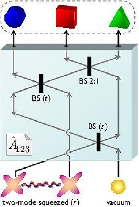
It is convenient in this instance to deal with the phase-space representations of the states (i.e. their CM) and of the operators (i.e. the associated symplectic transformations, see Sec. 6.2). The three-mode input state is described by a CM of the form Eq. (73) for , with [see Eq. (75)]
| (367) | |||||
| (368) |
and . A beam-splitter with transmittivity corresponds to a rotation of in phase space, see Eq. (78). In a three-mode system, the symplectic transformation corresponding to is a direct sum of the matrix , Eq. (79), acting on modes and , and of the identity acting on the remaining mode .
The output state after the allotment will be denoted by a CM given by
| (369) |
where is the phase-space representation of the allotment operator Eq. (366), obtained from the matrix product of the three beam-splitter transformations. The output state is clearly pure because the allotment is a unitary operator (symplectic in phase space). The elements of the CM , not reported here for brevity, are functions of the three parameters
| (370) |
being respectively related to the initial squeezing in the two-mode squeezed state of modes and , and two beam-splitter transmittivities (the transmittivity of the third beam-splitter is fixed). In fact, by letting these three parameters vary in their respective domain, the presented procedure allows for the creation of arbitrary three-mode pure Gaussian states (up to local unitaries), with any possible triple of local mixednesses ranging in the physical region defined by the triangle inequality (290).
This can be shown as follows. Once identified with the block form of Eq. (73) (for ), one can solve analytically the equation to find
| (371) |
Then, substituting Eq. (371) in yields a reparametrization of the output state in terms of (which is given), and . Now solve (numerically) the system of nonlinear equations in the variables and . Finally, substitute back the obtained values of the two transmittivities in Eq. (371), to have the desired triple as functions of the local mixednesses characterizing the target state.

We have therefore demonstrated the following [GA16].
- ➢
State engineering of pure three-mode Gaussian states. An arbitrary pure three-mode Gaussian state, with a CM locally equivalent to the standard form of Eq. (292), can be produced with the current experimental technology by linear quantum optics, employing the allotment box — a passive redistribution of two-mode entanglement among three modes — with exactly tuned amounts of input two-mode squeezing and beam-splitter properties, without any free parameter left.
A pictorial test of this procedure is shown in Fig. 36, where at a given local mixedness of mode (), several runs of the allotment operator have been simulated with randomized beam-splitter transmittivities and . Starting from a two-mode squeezed input with given by Eq. (371), tensor a vacuum, the resulting output states are plotted in the space of and . By comparing Fig. 36 with Fig. 17(b), one clearly sees that the randomly generated states distribute towards a complete fill of the physical region emerging from the triangle inequality (290), thus confirming the generality of our scheme.
29.2 Tripartite state engineering handbook and simplified schemes
Having a generalization of the “allotment” for the production of arbitrary mixed three-mode Gaussian states turns out to be a quite involved task. However, for many classes of tripartite states introduced in Chapter 7, efficient state engineering schemes can be devised. Also in special instances of pure states, depending in general on less than three parameters, cheaper recipes than the general one in terms of the allotment box are available. We will now complement the entanglement analysis of Secs. 23 and 24 with such practical proposals, as presented in Ref. [GA16].
29.2.1 CV GHZ/W states

Several schemes have been proposed to produce what we call finite-squeezing GHZ/ states of continuous variables, i.e. fully symmetric pure three-mode Gaussian states with promiscuous entanglement sharing (see Sec. 23.1). In particular, as discussed by van Loock and Braunstein [236], these states can be produced by mixing three squeezed beams through a double beam-splitter, or tritter [36]. One starts with mode squeezed in momentum, and modes and squeezed in position. In Heisenberg picture:
| (372) | |||||
| (373) |
where the suffix “0” refers to the vacuum. Then one combines the three modes in a tritter
| (374) |
where the action of an ideal (phase-free) beam-splitter operation on a pair of modes and is defined by Eq. (78).
The output of the tritter yields a CM of the form Eq. (113) with
| (375) | |||
| (376) |
This resulting pure and fully symmetric three-mode Gaussian state, obtained in general with differently squeezed inputs , is locally equivalent to the state prepared with all initial squeezings equal to the average (this will be discussed in more detail in connection with teleportation experiments, see Sec. 36).
The CM described by Eqs. (375,376) represents a CV GHZ/ state. It can be in fact transformed, by local symplectic operations, into the standard form CM given by Eq. (312), with
| (377) |
The preparation scheme of CV GHZ/ states is depicted in Fig. 37. It has been experimentally implemented [8], and the fully inseparability of the produced states has been verified through the violation of the separability inequalities derived in Ref. [240]. Very recently, the production of strongly entangled GHZ/ states has also been demonstrated by using a novel optical parametric oscillator, based on concurrent nonlinearities [34].
29.2.2 Noisy GHZ/W states
Noisy GHZ/ states, whose entanglement has been characterized in Sec. 24.2, can be obtained as GHZ/ states generated from (Gaussian) thermal states: one starts with three single-mode squeezed thermal states (with average photon number ) and combine them through a tritter Eq. (374), with the same procedure described in Fig. 37 for . The initial single, separable, modes are thus described by the following operators in Heisenberg picture,
| (378) | |||||
| (379) |
Defining , at the output of the tritter one obtains a CM of the form Eq. (113), with
| (380) | |||
| (381) |
This resulting CM is locally equivalent to the standard form of Eq. (325), with
| (382) |
Here is the same as in Eq. (326), and was indeed defined there by inverting Eq. (382).
Let us also mention again that noisy GHZ/ states would also result from the dissipative evolution of pure GHZ/ states in proper Gaussian noisy channels (see Sec. 24.1).
29.2.3 T states
The states have been introduced in Sec. 23.2 to show that in symmetric three-mode Gaussian states, imposing the absence of reduced bipartite entanglement between any two modes results in a frustration of the genuine tripartite entanglement. It may be useful to know how to produce this novel class of mixed Gaussian states in the lab.
The simplest way to engineer states is to reutilize the scheme of Fig. 37, i.e. basically the tritter, but with different inputs. Namely, one has mode squeezed again in momentum (with squeezing parameter ), but this time modes and are in a thermal state (with average photon number , depending on ). In Heisenberg picture:
| (383) | |||||
| (384) | |||||
| with |
Sending these three modes in a tritter Eq. (374) one recovers, at the output, a state whose CM is locally equivalent to the standard form of Eq. (23.2), with
| (385) |
29.2.4 Basset hound states
A scheme for producing the basset hound states of Sec. 24.3, and in general the whole family of pure bisymmetric Gaussian states known as “multiuser quantum channels” (due to their usefulness for telecloning, as we will show in Sec. 37), is provided in Ref. [238]. In the case of three-mode basset hound states of the form given by Eqs. (333,334), one can use a simplified version of the allotment introduced in Sec. 29.1 for arbitrary pure states. One starts with a two-mode squeezed state (with squeezing parameter ) of modes and , and mode in the single-mode vacuum, like in Eqs. (363–365).
Then, one combines one half (mode 2) of the two-mode squeezed state with the vacuum mode 3 via a 50:50 beam-splitter, described in phase space by , Eq. (79). The resulting three-mode state is exactly a basset hound state described by Eqs. (333,334), once one identifies . In a realistic setting, dealing with noisy input modes, mixed bisymmetric states can be obtained as well by the same procedure.
30 How to produce and exploit unlimited promiscuous entanglement?
In Chapter 8, four-mode Gaussian states with an unlimited promiscuous entanglement sharing have been introduced. Their definition, Eq. (339), involves three instances of a two-mode squeezing transformation of the form Eq. (77). From a practical point of view, two-mode squeezing transformations are basic tools in the domain of quantum optics [16], occurring e.g. in parametric down-conversions (see Sec. 28 for more technical details). Therefore, we can readily provide an all-optical preparation scheme for our promiscuous states [GA19], as shown in Fig. 38.

It is interesting to observe that the amount of producible squeezing in optical experiments is constantly improving [224]. Only technological, no a priori limitations need to be overcome to increase and/or to the point of engineering excellent approximations to the demonstrated promiscuous entanglement structure, elucidated in Chapter 8, in multimode states of light and atoms (see also [222]).
To make an explicit example, already with realistic squeezing degrees like and (corresponding to 3 dB and 10 dB, respectively, where decibels are defined in footnote 20 on page 20), one has a bipartite entanglement of ebits (corresponding to a Gaussian entanglement of formation [270], see Sec. 10.2, of ebits), coexisting with a residual multipartite entanglement of ebits, of which the tripartite portion is at most ebits. This means that one can simultaneously extract at least qubit singlets from each pair of modes and , and more than a single copy of genuinely four-qubit entangled states (like cluster states [192]). Albeit with imperfect efficiency, this entanglement transfer can be realized by means of Jaynes-Cummings interactions [176], representing a key step for a reliable physical interface between fields and qubits in a distributed quantum information processing network (see also Refs. [130, 216]).
Chapter 11 Efficient production of pure N-mode Gaussian states
Recently, a great insight into the role of entanglement in the description of quantum systems has been gained through the quantum information perspective, mostly focusing on the usefulness of entanglement, rather than on its meaning. In these years, quantum entanglement has turned from a paradoxical concept into a physical resource allowing for the encoding, manipulation, processing and distribution of information in ways forbidden by the laws of classical physics. In this respect, we have evidenced how CV entanglement between canonically conjugate observables of infinite-dimensional systems, like harmonic oscillators, light modes and atomic ensembles, has emerged as a versatile and powerful resource. In particular, multimode Gaussian states have been proven useful for a wide range of implementations in CV quantum information processing [40], and advances in the characterization of their bipartite and multipartite entanglement have been recently recorded (see the previous Parts of this Dissertation).
In experiments, one typically aims at preparing pure states, with the highest possible entanglement, even though unavoidable losses and thermal noises will affect the purity of the engineered resources, and hence the efficiency of the realized protocols (a direct evidence is reported in Sec. 28). It is therefore important to understand the structure of correlations in pure Gaussian states of an arbitrary number of modes, and to provide economical schemes to produce such states in the lab with minimal elements, thus reducing the possibility of accumulating errors and unwanted noise.
31 Degrees of freedom of pure Gaussian states: practical perspectives
In the instance of two- and three-mode Gaussian states, efficient schemes for their optical production with minimal resources have been presented, respectively, in Chapters 9 and 10. In the general case of pure -mode Gaussian states with , we know from Eq. (109) that the minimal number of degrees of freedom characterizing all their structural and informational properties (up to local unitaries) is (see also Sec. 8.2 and Appendix 15).
It would be desirable to associate the mathematically clear number with an operational, physical insight. In other words, it would be useful for experimentalists (working, for instance, in quantum optics) to be provided with a recipe to create pure -mode Gaussian states with completely general entanglement properties in an economical way, using exactly optical elements, such as squeezers, beam-splitters and phase shifters. A transparent approach to develop such a procedure consists in considering the reverse of the phase space Schmidt decomposition, as introduced in Sec. 8.2.1. Namely, a completely general (not accounting for the local invariances) state engineering prescription for pure Gaussian states can be cast in two main steps: (i) create a two-mode squeezed state of modes 1 and 2, which corresponds to the multimode state in its Schmidt form; (ii) operate with the most general -mode symplectic transformation on the block of modes (with modes initially in the vacuum state) to redistribute entanglement among all modes. The operation is the inverse of the transformation which brings the reduced CM of modes in its Williamson diagonal form, see Sec. 6.2.1. It is also known that any such symplectic transformation (unitary on the Hilbert space) can be decomposed in a network of optical elements [193]. The number of elements required to accomplish this network, however, will in general greatly exceed the minimal number of parameters on which the entanglement between any two sub-systems depends. Shifting the local-unitary optimization from the final CM, back to the engineering symplectic network, is in principle an extremely involved and nontrivial task.
This problem has been solved in Ref. [GA14] for a special subclass of Gaussian states, which is of null measure but still of central importance for practical implementations. It is constituted by those pure -mode Gaussian states which can be locally put in a standard form with all diagonal submatrices in Eq. (73) (i.e. with null in the notation of Appendix 15). This class encompasses generalized GHZ-type Gaussian states, useful for CV quantum teleportation networks [236] (see Sec. 36), Gaussian cluster states [280, 242] employed in CV implementations of one-way quantum computation [155], and states of four or more modes with an unlimited promiscuous entanglement sharing (see Chapter 8). It also comprises (as proven in Sec. 21.2) all three-mode pure Gaussian states, whose usefulness for CV quantum communication purposes has been thoroughly investigated in this Dissertation (see Chapter 7, Chapter 10, and Sec. 37). In the physics of many-body systems, those states are quite ubiquitous as they are ground states of harmonic Hamiltonians with spring-like interactions [11]. As such, they admit an efficient “valence bond” description, as discussed in Chapter 13.
For these Gaussian states, which we will call here block-diagonal — with respect to the canonical operators reordered as — the minimal number of local-unitarily-invariant parameters reduces to for any .2828 28 This number is easily derived from the general framework developed in Appendix 15.B: for , Eqs. (481) and (482) reduce to . The only further condition to impose after the local reduction is then , which brings the number of free parameters of the symmetric from down to . Accordingly, one can show that an efficient scheme can be devised to produce block-diagonal pure Gaussian states, involving exactly optical elements which in this case are only constituted by single-mode squeezers and beam-splitters, in a given sequence [GA14].
We will now detail the derivation of these results explicitly, as it will lead to an important physical insight into the entanglement structure (which we define “generic”) of such block-diagonal Gaussian states. The latter, we recall, are basically all the resources currently produced and employed in optical realizations of CV quantum information and communication processing.
32 Generic entanglement, standard form and state engineering of block-diagonal pure Gaussian states
32.1 Generic entanglement of Gaussian states
In this Section, based on Ref. [GA14] we address the question of how many physical resources are really needed to engineer and characterize entanglement in pure Gaussian states of an arbitrary number of modes, up to local unitary operations. Let us recall again (see Sec. 8.2) that for states of modes, it has been shown that such a number of minimal degrees of freedom scales as . For a higher number of modes, however, a richer structure is achievable by pure Gaussian states, as from symplectic arguments like those of Appendix 15.B.1 a minimal number of parameters given by can be inferred. A random state of modes, selected according to the uniform distribution over pure Gaussian states, will be thus reducible to a form characterized by such a number of independent quantities.
However, in practical realizations of CV quantum information one is interested in states which, once prepared with efficient resources, still achieve an almost complete structural variety in their multipartite entanglement properties. Such states will be said to possess generic entanglement [166], where generic means practically equivalent to that of random states, but engineered (and described) with a considerably smaller number of degrees of freedom.
Precisely, we define as “generic-entangled” those Gaussian states whose local entropies of entanglement in any single mode are independent, and bipartite entanglements between any pair of modes are unconstrained. Having a standard form for such -mode Gaussian states, may be in fact extremely helpful in understanding and quantifying multipartite CV entanglement, in particular from the theoretical point of view of entanglement sharing and monogamy constraints (see Chapter 6), and from a more pragmatical approach centered on using entanglement as a resource.
We show that, to achieve generic entanglement, for the global pure -mode Gaussian state it is enough to be described by a minimal number of parameters (corresponding to the local-unitarily invariant degrees of freedom) equal to for any , and thus much smaller than the of a completely general CM. Therefore, generic entanglement appears in states which are highly not ‘generic’ in the sense usually attributed to the term, i.e. randomly picked. Crucially, we demonstrate that “generic-entangled” Gaussian states coincide with the above defined “block-diagonal” Gaussian states, i.e. with the resources typically employed in experimental realizations of CV quantum information [40]. Accordingly, we provide an optimal and practical scheme for their state engineering.
32.2 Minimal number of parameters
Adopting the above definition of generic entanglement, we prove now the main
Proposition 1
A generic-entangled -mode pure Gaussian state is described, up to local symplectic (unitary) operations, by independent parameters.
Proof. Let us start with a -mode pure state, described by a CM as in Eq. (73), with all single-mode blocks () in diagonal form: we can always achieve this by local single-mode Williamson diagonalizations in each of the modes. Let be the reduced CM of modes . It can be diagonalized by means of a symplectic , and brought thus to its Williamson normal form, characterized by a symplectic spectrum , where . Transforming by , brings the CM into its Schmidt form, constituted by a two-mode squeezed state between modes and (with squeezing ), plus vacua [116, 29, 92] (see Sec. 8.2.1).
All -mode pure Gaussian states are thus completely specified by the symplectic , plus the parameter . Alternatively, the number of parameters of is also equal to that characterizing an arbitrary mixed -mode Gaussian CM, with symplectic rank (i.e. with symplectic eigenvalues equal to , see Sec. 6.2.2). This means that, assigning the reduced state , we have provided a complete description of . In fact, the parameter is determined as the square root of the determinant of the CM .
We are now left to compute the minimal set of parameters of an arbitrary mixed state of modes, with symplectic rank . While we know that for this number is equal to in general, we want to prove that for generic-entangled Gaussian resource states this number reduces to
| (386) |
We prove it by induction. For a pure state of one mode only, there are no reduced “zero-mode” states, so the number is zero. For a pure state of two modes, an arbitrary one-mode mixed CM with is completely determined by its own determinant, so the number is one. This shows that our law for holds true for and .
Let us now suppose that it holds for a generic , i.e. we have that a mixed -mode CM with can be put in a standard form specified by parameters. Now let us check what happens for a -mode pure state, i.e. for the reduced -mode mixed state with symplectic rank equal to . A general way (up to LUs) of constructing a -mode CM with yielding generic entanglement is the following: (a) take a generic-entangled -mode CM with in standard form; (b) append an ancillary mode () initially in the vacuum state (the mode cannot be thermal as must be preserved); (c) squeeze mode with an arbitrary (one has this freedom because it is a local symplectic operation); (d) let mode interact couplewise with all the other modes, via a chain of beam-splitters, Eq. (79), with arbitrary transmittivities , with ;2929 29 Squeezings and beam-splitters are basic entangling tools in CV systems, see Sec. 6.2. For , steps (c) and (d) should be generalized to arbitrary one- and two-mode symplectic transformations to achieve all possible Gaussian states, as discussed in Sec. 31. (e) if desired, terminate with suitable single-mode squeezing operations (but with all squeezings now fixed by the respective reduced CM’s elements) to symplectically diagonalize each single-mode CM.
With these steps one is able to construct a mixed state of modes, with the desired rank, and with generic (local-unitarily-invariant) properties for each single-mode individual CM. We will show in the following that in the considered states the pairwise quantum correlations between any two modes are unconstrained. To conclude, let us observe that the constructed generic-entangled state is specified by a number of parameters equal to: (the parameters of the starting -mode mixed state of the same form) plus (the initial squeezing of mode ) plus (the two-mode beam-splitter interactions between mode and each of the others). Total: .
32.3 Quantum state engineering
Following the ideas of the above proof, a physically insightful scheme to produce generic-entangled -mode pure Gaussian states can be readily presented (see Fig. 39). It consists of basically two main steps: (1) creation of the state in the Schmidt decomposition; (2) addition of modes and entangling operations between them. One starts with a chain of vacua.
First of all (step 1), the recipe is to squeeze mode of an amount , and mode 2 of an amount (i.e. one squeezes the first mode in one quadrature and the second, of the same amount, in the orthogonal quadrature); then one lets the two modes interfere at a beam-splitter. One has so created a two-mode squeezed state between modes and (as in Fig. 26), which corresponds to the Schmidt form of with respect to the bipartition. The second step basically corresponds to create the most general mixed state with , of modes , out of its Williamson diagonal form. This task can be obtained, as already sketched in the above proof, by letting each additional mode interact step-by-step with all the previous ones. Starting with mode (which was in the vacuum like all the subsequent ones), one thus squeezes it (of an amount ) and combines it with mode via a beam-splitter , Eq. (79) (characterized by a transmittivity ). Then one squeezes mode by and lets it interfere sequentially, via beam-splitters, both with mode (with transmittivity ) and with mode (with transmittivity ). This process can be iterated for each other mode, as shown in Fig. 39, until the last mode is squeezed () and entangled with the previous ones via beam-splitters with respective transmittivities , . Step 2 describes the redistribution of the two-mode entanglement created in step 1, among all modes. We remark that mode becomes entangled with all the other modes as well, even if it never comes to a direct interaction with each of modes .

The presented prescription enables to create a generic form (up to local unitaries) of multipartite entanglement among modes in a pure Gaussian state, by means of active (squeezers) and passive (beam-splitters) linear optical elements. What is relevant for practical applications, is that the state engineering is implemented with minimal resources. Namely, the process is characterized by one squeezing degree (step 1), plus individual squeezings for step 2, together with beam-splitter transmittivities, which amount to a total of quantities. The optimally produced Gaussian states can be readily implemented for -party CV communication networks (see Chapter 12).
A remark is in order. From Eq. (109), it follows that the scheme of Fig. 39, in the special case , allows for the creation of all pure three-mode Gaussian states with CM in standard form, Eq. (292). In other words, up to local unitaries, all pure three-mode Gaussian states exhibit generic entanglement as defined above. Therefore, the state engineering recipe presented here represents an alternative to the allotment box of Fig. 35, introduced in Sec. 29.1. In both schemes, the input is a two-mode squeezed state of modes 1 and 2 (whose squeezing degree accounts for one of the three degrees of freedom of pure three-mode Gaussian states, see Sec. 21.2) and mode 3 in the vacuum state. The main difference is that in the present scheme (Fig. 39), an additional active operation is implemented, as the third mode is squeezed in the first place; a single beam-splitter (between modes 2 and 3) is then enough to achieve a completely general entanglement structure in the three modes, up to local unitaries. On the other hand, the allotment of Fig. 35, as the name itself suggests, is realized by a passive redistribution of entanglement only, as the third mode is not squeezed but the three modes interfere with each other via three beam-splitters (one of which has fixed transmittivity) and this again yields a completely general entanglement freedom, up to local unitaries. Depending on the experimental facilities, one can thus choose either scheme when aiming to produce pure three-mode Gaussian states.
32.4 Standard forms: generic-entangled ↔ block-diagonal
The special subset of pure -mode Gaussian states emerging from our constructive proof exhibits a distinct property: all correlations between “position” and “momentum” operators are vanishing. Looking at Eq. (73), this means that any such generic-entangled pure Gaussian state can be put in a standard form where all the submatrices of its CM are diagonal. The class of pure Gaussian states exhibiting generic entanglement coincides thus with that formed by the “block-diagonal” states discussed in Secs. 8.2 and 31.
The diagonal subblocks can be additionally made proportional to the identity by local Williamson diagonalizations in the individual modes. This standard form for generic-entangled -mode Gaussian states, as already mentioned, can be achieved by all pure Gaussian states for [70] and [GA11] (see Sec. 21.2); for , pure Gaussian states can exist whose number of independent parameters scales as and which cannot thus be brought in the - block-diagonal form. Interestingly, all pure Gaussian states in our considered block-diagonal standard form, are ground states of quadratic Hamiltonians with spring-like interactions [11]. Let us now investigate the physical meaning of the standard form.
Vanishing - covariances imply that the -mode CM can be written as a direct sum (see also Appendix 15) , when the canonical operators are arranged as . Moreover, the global purity of imposes . Named and , this means that each is a function of the ’s. The additional Williamson conditions fix the diagonal elements of . The standard form is thus completely specified by the off-diagonal elements of the symmetric matrix , which are, as expected, from Eq. (386).
- ➢
Generic entanglement of pure Gaussian states. The structural properties of pure block-diagonal -mode Gaussian states, and in particular their bipartite and multipartite entanglement, are completely specified (up to local unitaries) by the ‘two-point correlations’ between any pair of modes, which amount to locally invariant degrees of freedom.
For instance, the entropy of entanglement between one mode (say ) and the remaining modes, which is monotonic in (see Sec. 7), is completely specified by assigning all the pairwise correlations between mode and any other mode , as from Eq. (108). The rationale is that entanglement in such states is basically reducible to a mode-to-mode one. This statement, strictly speaking true only for the pure Gaussian states for which Proposition 1 holds, acquires a general validity in the context of the modewise decomposition of arbitrary pure Gaussian states [116, 29, 92], as detailed in Sec. 8.2.1. We remark that such an insightful correlation picture breaks down for mixed Gaussian states, where also classical, statistical-like correlations arise.
33 Economical state engineering of arbitrary pure Gaussian states?
Borrowing the ideas leading to the state engineering of block-diagonal pure Gaussian states [GA14], see Fig. 39, we propose here a scheme [GA18], involving independent optical elements, to produce more general -mode pure Gaussian states, encoding correlations between positions and momentum operators as well. To this aim, we introduce ‘counter-beam-splitter’ transformations, named “seraphiques”, which, recovering the phase space ordering of Sec. 5, act on two modes and as
| (387) |
where the amplitude is related to an angle in phase space by . Such operations can be obtained from usual beam-splitters , Eq. (79), by applying a phase shifter on only one of the two considered modes. is a local rotation mapping, in Heisenberg picture, and . In phase space, one has . Notice that, even though is equal to the product of single-mode operations and beam-splitters, this does not mean that such a transformation is “equivalent” to a beam-splitter in terms of state generation. In fact, the local operations do not commute with the beam-splitters, so that a product of the kind cannot be written as for some local operation and .

The state engineering scheme runs along exactly the same lines as the one for the block-diagonal states, Sec. 32.3, the only modification being that for each pair of modes except the last one (), a beam-splitter transformation is followed by a seraphique. In more detail (see Fig. 40): first of all (step 1), one squeezes mode of an amount , and mode of an amount (i.e. one squeezes the first mode in one quadrature and the second, of the same amount, in the orthogonal quadrature); then one lets the two modes interfere at a beam-splitter. One has so created a two-mode squeezed state between modes and , which corresponds to the Schmidt form of the pure Gaussian state with respect to the bipartition. The second step basically corresponds to a re-distribution of the initial two-mode entanglement among all modes; this task can be obtained by letting each additional mode () interact step-by-step with all the previous ones (), via beam-splitters and seraphiques (which are in turn combinations of beam-splitters and phase shifters). It is easy to see that this scheme is implemented with minimal resources. Namely, the state engineering process is characterized by one squeezing degree (step 1), plus individual squeezings, together with beam-splitter transmittivities, and seraphique amplitudes, which amount to a total of quantities, exactly the ones parametrizing a generic pure Gaussian state of modes up to local symplectic operations, Eq. (109).
While this scheme (Fig. 40) is surely more general than the one for block-diagonal states (Fig. 39), as it enables to efficiently create a broader class of pure Gaussian states for , we will leave it as an open question to check if it is general enough to produce all pure -mode Gaussian states up to local unitaries. Verifying this analytically leads to pretty intractable expressions already for . Instead, it would be very interesting to investigate if the average entanglement of the output Gaussian states numerically obtained by a statistically significant sample of applications of our scheme with random parameters, matches the typical entanglement of pure Gaussian states under “thermodynamical” state-space measures as computable along the lines of Ref. [209]. This would prove the optimality and generality of our scheme in an operational way, which is indeed more useful for practical applications.
34 Generic versus typical entanglement: are off-block-diagonal correlations relevant?
The structural properties of pure -mode Gaussian states under local operations have been addressed in Sec. 8.2 and completely characterized in Appendix 15 [GA18]. Here [GA14], block-diagonal states (i.e. with no correlations between position and momentum operators) have been in particular proven to possess generic entanglement in the sense of Sec. 32.1, and their standard form covariances (determining any form of entanglement in such states) have been physically understood in terms of two-body correlations. It is thus quite natural to question if the additional parameters encoded in - correlations for non-block-diagonal pure states, have a definite impact or not on the bipartite and multipartite entanglement.
At present, usual CV protocols are devised, even in multimode settings (see Chapter 12), to make use of states without any - correlations. In such cases, the economical (relying on parameters) “block-diagonal state engineering” scheme detailed in Fig. 39 is clearly the optimal general strategy for the production of entangled resources. However, theoretical considerations strongly suggest that states with [adopting the notation of Eq. (480)] might have remarkable potential for improved quantum-informational applications. In fact, considering as just mentioned the thermodynamical entanglement framework of Gaussian states [209], one can define natural averages either on the whole set of pure Gaussian states, or restricting to states with . Well, numerics unambiguously show [GA18] that the (thermodynamically-averaged) “generic” entanglement (under any bipartition) of Gaussian states without - correlations (like the ones considered in Sec. 32.1) is systematically lower than the “typical” entanglement of completely general pure Gaussian states, with this behavior getting more and more manifest as the total number of modes increases (clearly, according to Sec. 8.2, this discrepancy only arises for ). In a way, the full entanglement potential of Gaussian states is diminished by the restriction to block-diagonal states.
On the other hand, the comparison between the average entanglement generated in randomizing processes based on the engineering scheme of Fig. 40, and the block-diagonal one of Fig. 39, is under current investigation as well. If the general scheme of Fig. 40, based on beam-splitters and seraphiques, turned out to be out-performing the simpler ones (like the one of Fig. 39, based on beam-splitters only) in terms of entanglement generation — as expected in view of the argument above — this would provide us with a formidable motivation to explore novel CV protocols capable of adequately exploiting - correlated resources.
Part V Operational interpretation and applications of Gaussian entanglement
![[Uncaptioned image]](0702069v1/entanglement_manycubes.png)
Entanglement. Anne Kesler
Shields, 2004.
http://annekeslershields.com/portfolio/port10.html
Chapter 12 Multiparty quantum communication with Gaussian resources
The field of quantum information with continuous variables is flourishing with theoretical and experimental successes. It can be considered mature for what concerns two-party information and communication processing, exploiting in particular bipartite entangled resources such as two-mode Gaussian states. We have ourselves contributed some experimental results on the production and manipulation of two-mode entanglement in Gaussian optical beams (see Sec. 28). An in-depth excursus in this multifaceted physical sector is beyond the scope of the present Dissertation, and the interested reader may surely find a comprehensive and quite up-to-date review on the subject in Ref. [40].
In this Part, having laid the foundations for a proper quantification of multipartite entanglement in CV system in Part III, and having dealt with the issue of efficiently producing multipartite entangled resources in practical optical settings in Part IV, we judge a wise choice to collect our results concerning the usefulness and optimal exploitation of Gaussian entanglement for processes involving more than two parties. We will also include in this Part applications of our machinery to study the structure and distribution of correlations in harmonic lattices with an underlying valence bond structure (Chapter 13), as well as to investigate entanglement sharing between non-inertial observers in a relativistic setting (Chapter 14).
We begin in this Chapter by epitomizing the capability of Gaussian states for quantum communication and by providing their theoretical entanglement characterization with a significant operative background. To this aim we will focus on the transmission of quantum states by means of classical communication and entangled Gaussian resources shared by parties: specifically, CV teleportation networks and telecloning.
35 Quantum teleportation with continuous variables
For two parties, the process of quantum teleportation using entanglement and with the aid of classical communication was originally proposed for qubit systems [22], and experimentally implemented with polarization-entangled photons [31, 27].
The CV counterpart of discrete-variable teleportation, using quadrature entanglement, is in principle imperfect due to the impossibility of achieving infinite squeezing. Nevertheless, by considering the finite EPR correlations between the quadratures of a two-mode squeezed Gaussian state, Eq. (75), a realistic scheme for CV teleportation was proposed [234, 39] and experimentally implemented to teleport coherent states with a measured fidelity up to [89, 33, 226]. Without using entanglement, by purely classical communication, an average fidelity of
| (388) |
is the best that can be achieved if the alphabet of input states includes all coherent states with even weight [38, 107]. Let us recall that the fidelity , which is the figure of merit quantifying the success of a teleportation experiment, is defined with respect to a pure state as
| (389) |
Here “in” and “out” denote the input and the output states (the latter being generally mixed) of a teleportation process, respectively. reaches unity only for a perfect state transfer, . To accomplish teleportation with high fidelity, the sender (Alice) and the receiver (Bob) must share an entangled state (resource). The sufficient fidelity criterion [38] states that, if teleportation is performed with , then the two parties exploited an entangled state. The converse is generally false, that is, quite surprisingly, some entangled resources may in principle yield lower-than-classical fidelities. This point will be discussed thoroughly in the following and the solution to such a puzzling issue, obtained in [GA9], will be explained.
Let us briefly mention how to compute Eq. (389), in terms of CMs. Setting, as usual, all first moments to zero, the fidelity of two-user teleportation of arbitrary single-mode Gaussian states exploiting two-mode Gaussian resources can be computed directly from the respective second moments [206]. Being the CM of the unknown input state, and
| (390) |
the CM of the shared two-mode resource, and defining the matrix , the fidelity reads [206]
| (391) |
We will exploit this formula in the following.
To generalize the process of CV teleportation from two to three and more users, one can consider two basic possible scenarios. On the one hand, a network can be created where each user is able to teleport states with better-than-classical efficiency (being the same for all sender/receiver pairs) to any chosen receiver with the assistance of the other parties. On the other hand, one of the parties acts as the fixed sender, and distributes many approximate copies (with in principle different cloning fidelities) to all the others acting as remote receivers. These two protocols, respectively referred to as “teleportation network” [236] and “telecloning” [238], will be described in the two following sections, and the connections between their successful implementation with multimode Gaussian resources and the amounts of shared bipartite and multipartite entanglement, as obtained in Refs. [GA9, GA16], will be elucidated. We just mention that several interesting variants to these basic schemes do exist, (see e.g., in a tripartite setting, the ‘cooperative telecloning’ of Ref. [181], where two receivers, instead of two senders, are cooperating).
36 Equivalence between entanglement in symmetric Gaussian resource states and optimal nonclassical teleportation fidelity
The original CV teleportation protocol [39] has been generalized to a multi-user teleportation network requiring multiparty entangled Gaussian states in Ref. [236]. The tripartite instance of such a network has been recently experimentally demonstrated by exploiting three-mode squeezed states, yielding a maximal fidelity of [277].
Here, based on Ref. [GA9], we investigate the relation between the fidelity of a CV teleportation experiment and the entanglement present in the shared resource Gaussian states. We find in particular that, while all the states belonging to the same local-equivalence class (i.e. convertible into each other by local unitary operations) are undistinguishable from the point of view of their entanglement properties, they generally behave differently when employed in quantum information and communication processes, for which the local properties such as the optical phase reference get relevant. Hence we show that the optimal teleportation fidelity, maximized over all local single-mode unitary operations (at fixed amounts of noise and entanglement in the resource), is necessary and sufficient for the presence of bipartite (multipartite) entanglement in two-mode (multimode) Gaussian states employed as shared resources. Moreover, the optimal fidelity allows for the quantitative definition of the entanglement of teleportation, an operative estimator of bipartite (multipartite) entanglement in CV systems. Remarkably, in the multi-user instance, the optimal shared entanglement is exactly the “localizable entanglement”, originally introduced for spin systems [248] (not to be confused with the unitarily localizable entanglement of bisymmetric Gaussian states, discussed in Chapter 5), which thus acquires for Gaussian states a suggestive operative meaning in terms of teleportation processes. Moreover, let us recall that our previous study on CV entanglement sharing led to the definition of the residual Gaussian contangle, Eq. (309), as a tripartite entanglement monotone under Gaussian LOCC for three-mode Gaussian states [GA10] (see Sec. 22.2). This measure too is here operationally interpreted via the success of a three-party teleportation network.
Besides these fundamental theoretical results, our findings are of important practical interest, as they answer the experimental need for the best preparation recipe for entangled squeezed resources, in order to implement CV teleportation (in the most general setting) with the highest fidelity. It is indeed crucial in view of experimental implementations, to provide optimal ways to engineer quantum correlations, such that they are not wasted but optimally exploited for the specifical task to be realized. We can see that this was the leitmotiv of the previous Chapter as well.
We will now detail the results obtained in Ref. [GA9], starting with the two-party teleportation instance, and then facing with the general (and more interesting) -party teleportation network scenario. Notice that, by the defining structure itself of the protocols under consideration, the employed resources will be (both in the two-party and in the general -party case) fully symmetric, generally mixed Gaussian states (see Sec. 8.3). Therefore the equivalence between optimal nonclassical fidelity and entanglement strictly holds only for fully symmetric Gaussian resources. We will discuss this thoroughly in the following, and show how this interesting connection actually is not valid anymore for nonsymmetric, even two-mode resources.
36.1 Optimal fidelity of two-party teleportation and bipartite entanglement
The two-user CV teleportation protocol [39] would require, to achieve unit fidelity, the sharing of an ideal (unnormalizable) EPR resource state [73], i.e. the simultaneous eigenstate of relative position and total momentum of a two-mode radiation field. An arbitrarily good approximation of the EPR state, as we know, is represented by two-mode squeezed Gaussian states of Eq. (75) with squeezing parameter .
As remarked in Sec. 28, a two-mode squeezed state can be, in principle, produced by mixing a momentum-squeezed state and a position-squeezed state, with squeezing parameters and respectively, through a 50:50 ideal (lossless) beam-splitter. In practice, due to experimental imperfections and unavoidable thermal noise the two initial squeezed states will be mixed. To perform a realistic analysis, we must then consider two thermal squeezed single-mode states,3030 30 Any losses due to imperfect optical elements and/or to the fibre or open-air propagation of the beams can be embedded into the initial single-mode noise factors. described by the following quadrature operators in Heisenberg picture
| (392) | |||||
| (393) |
where the suffix “0” refers to the vacuum. The action of an ideal (phase-free) beam-splitter operation on a pair of modes and , corresponding to a phase-space rotation of an angle , is defined by Eq. (78).

When applied to the two modes of Eqs. (392,393), the beam-splitter entangling operation () produces a symmetric mixed state [131], depending on the squeezings and on the thermal noises , as depicted in Fig. 41. The CM of such a state reads
| (394) |
The noise can be difficult to control and reduce in the lab, but we assume it is at least quantifiable (see Sec. 28). Now, keeping and fixed, all states produced starting with different and , but with equal average
| (395) |
are completely equivalent up to local unitary operations and possess, by definition, the same entanglement. Let us recall that, as we are dealing with symmetric two-mode Gaussian states, all conceivable entanglement quantifications are equivalent, including the computable entanglement of formation (see Sec. 12.2), and are all decreasing functions of the smallest symplectic eigenvalue of the partially transposed CM, computable as in Eq. (142).
For the mixed two-mode states considered here, we have
| (396) |
The entanglement thus depends both on the arithmetic mean of the individual squeezings, and on the geometric mean of the individual noises, which is related to the purity of the state . The teleportation success, instead, depends separately on each of the four single-mode parameters. The fidelity Eq. (389) (averaged over the complex plane) for teleporting an unknown single-mode coherent state can be computed by writing the quadrature operators in Heisenberg picture [236, 235],
| (397) |
where and are the variances of the canonical operators and which describe the teleported mode. For the utilized states, we have
| (398) |
where the suffix “in” refers to the input coherent state to be teleported. Recalling that, in our units (see Sec. 5), , we can compute the fidelity from Eq. (397), obtaining
It is convenient to replace and by , Eq. (395), and
| (399) |
One has then
| (400) |
Maximizing the fidelity, Eq. (397), for given entanglement and noises of the Gaussian resource state (i.e. for fixed ) simply means finding the which minimizes the quantity of Eq. (400). Being a convex function of , it suffices to find the zero of , which yields an optimal given by
| (401) |
For equal noises (), , indicating that the best preparation of the entangled resource state needs two equally squeezed single-mode states, in agreement with the results presented in Ref. [32] for pure states. For different noises, however, the optimal procedure involves two different squeezings, biased such that . Inserting from Eq. (401), in Eq. (400), we have the optimal fidelity
| (402) |
where is exactly the smallest symplectic eigenvalue of the partial transpose of the CM , Eq. (394), defined by Eq. (396).
Eq. (402) clearly shows that the optimal teleportation fidelity depends only on the entanglement of the resource state, and vice versa. In fact, the fidelity criterion becomes necessary and sufficient for the presence of the entanglement, if is considered: the optimal fidelity is classical for (separable state) and it exceeds the classical threshold for any entangled state. Moreover, provides a quantitative measure of entanglement completely equivalent to the negativities and to the two-mode entanglement of formation [GA9]. Namely, from Eqs. (146,402),
| (403) |
with defined by Eq. (147). In the limit of infinite squeezing (), reaches for any amount of finite thermal noise.
On the other extreme, due to the convexity of , the lowest fidelity is attained at one of the boundaries, . Explicitly, the worst teleportation success, corresponding to the maximum waste of bipartite entanglement, is achieved by encoding zero squeezing in the more mixed mode, i.e. if , and otherwise. For infinite squeezing, the worst fidelity cannot exceed , easily falling below the classical bound for strong enough noise.
36.2 Optimal fidelity of N-party teleportation networks and multipartite entanglement
We now extend our analysis [GA9] to a quantum teleportation-network protocol, involving users who share a genuine -partite entangled Gaussian resource, fully symmetric under permutations of the modes [236] (see Sec. 8.3 for the analysis of fully symmetric Gaussian states).
Two parties are randomly chosen as sender (Alice) and receiver (Bob), but this time, in order to accomplish teleportation of an unknown coherent state, Bob needs the results of momentum detections performed by the other cooperating parties. A nonclassical teleportation fidelity (i.e. ) between any pair of parties is sufficient for the presence of genuine -partite entanglement in the shared resource, while in general the converse is false [see e.g. Fig. 1 of Ref. [236], reproduced in Fig. 43(b)]. Our aim is to determine the optimal multi-user teleportation fidelity, and to extract from it a quantitative information on the multipartite entanglement in the shared resources.
We begin with the state engineering of the shared -partite resource. Let us consider, generalizing Sec. 36.1, a mixed momentum-squeezed state described by as in Eq. (392), and position-squeezed states of the form Eq. (393),
| (404) | |||||
| (405) |
with . We then combine the beams into an -splitter, which is a sequence of suitably tuned beam-splitters [236]:
| (406) |
where the unitary beam-splitter operator acting on modes and is defined by Eq. (78). Eq. (406) represents the generalization to modes of the “tritter”, Eq. (374).
The resulting state (see Fig. 42) is a completely symmetric mixed Gaussian state of a -mode CV system, with a CM of the form Eq. (113), parametrized by , and . Once again, all states with equal belong to the same iso-entangled class of equivalence, up to local unitaries. For and for (pure states), these states reproduce the (unnormalizable) CV generalized GHZ state, , an eigenstate with total momentum and all relative positions ().

Choosing randomly two modes, denoted by the indices and , to be respectively the sender and the receiver, the teleported mode is described by the following quadrature operators (see Refs. [236, 235] for further details):
| (407) |
with
| (408) |
where is an experimentally adjustable gain. To compute the teleportation fidelity from Eq. (397), we need the variances of the operators and of Eq. (408). From the action of the -splitter, Eq. (406), we find
| (409) | |||||
The optimal fidelity can be now found in two straightforward steps: 1) minimizing with respect to (i.e. finding the optimal gain ); 2) minimizing the resulting with respect to (i.e. finding the optimal bias ). The results are
| (410) | |||||
| (411) |
Inserting Eqs. (36.2–411) in Eq. (397), we find the optimal teleportation-network fidelity, which can be put in the following general form for modes
| (412) |
For , from Eq. (396), showing that the general multipartite protocol comprises the standard bipartite one as a special case.

By comparison with Eq. (402), we observe that, for any , the quantity plays the role of a “generalized symplectic eigenvalue”, whose physical meaning will be clear soon. Before that, it is worth commenting on the form of the optimal resources, focusing for simplicity on the pure-state setting (). The optimal form of the shared -mode symmetric Gaussian states, for , is neither unbiased in the and quadratures (like the states discussed in Ref. [32] for three modes), nor constructed by equal squeezers (). This latter case, which has been implemented experimentally for [277], is clearly not optimal, yielding fidelities lower than for and falling in a certain interval [236] [see Fig. 43(b)]. The explanation of this paradoxical behavior, provided by the authors of Ref. [236], is that their teleportation scheme might not be optimal. Our analysis [GA9] shows instead that the problem does not lie in the choice of the protocol, but rather in the form of the employed states. If the shared -mode resources are prepared by suitable pre-processing — or transformed by local unitary (symplectic on the CM) operations — into the optimal form of Eq. (411), the teleportation fidelity is guaranteed to be nonclassical [see Fig. 43(a)] as soon as for any , in which case the considered class of pure states is genuinely multiparty entangled (we have shown this unambiguously in Sec. 18). Therefore, we can state the following [GA9].
- ➢
Equivalence between entanglement and optimal fidelity of continuous variable teleportation. A nonclassical optimal fidelity is necessary and sufficient for the presence of multipartite entanglement in any multimode symmetric Gaussian state, shared as a resource for CV teleportation networks.
This equivalence silences the embarrassing question that entanglement might not be an actual physical resource, as protocols based on some entangled states might behave worse than their classical counterparts in processing quantum information.
On the opposite side, the worst preparation scheme of the multimode resource states, even retaining the optimal protocol (), is obtained setting if , and otherwise. For equal noises (), the case is always the worst one, with asymptotic fidelities (in the limit ) equal to , and so rapidly dropping with at given noise.
36.2.1 Entanglement of teleportation and localizable entanglement
The meaning of , Eq. (412), crucial for the quantification of the multipartite entanglement, stems from the following argument. The teleportation network [236] is realized in two steps: first, the cooperating parties perform local measurements on their modes, then Alice and Bob exploit their resulting highly entangled two-mode state to accomplish teleportation. Stopping at the first stage, the protocol describes a concentration, or localization of the original -partite entanglement, into a bipartite two-mode entanglement [236, 235]. The maximum entanglement that can be concentrated on a pair of parties by locally measuring the others, is known as the localizable entanglement3131 31 This localization procedure, based on measurements, is different from the unitary localization which can be performed on bisymmetric Gaussian states, as discussed in Chapter 5. of a multiparty system [248], as depicted in Fig. 44.
Here, the localizable entanglement is the maximal entanglement concentrable onto two modes, by unitary operations and nonunitary momentum detections performed locally on the other modes. The two-mode entanglement of the resulting state (described by a CM ) is quantified in general in terms of the symplectic eigenvalue of its partial transpose. Due to the symmetry of both the original state and the teleportation protocol (the gain is the same for every mode), the localized two-mode state will be symmetric too. We have shown in Sec. 12.3 that, for two-mode symmetric Gaussian states, the symplectic eigenvalue is related to the EPR correlations by the expression [GA3]
For the state , this means , where the variances have been computed in Eq. (36.2). Minimizing with respect to means finding the optimal set of local unitary operations (unaffecting multipartite entanglement) to be applied to the original multimode mixed resource described by ; minimizing then with respect to means finding the optimal set of momentum detections to be performed on the transformed state in order to localize the highest entanglement on a pair of modes. From Eq. (36.2), the optimizations are readily solved and yield the same optimal and of Eqs. (410,411).
The resulting optimal two-mode state contains a localized entanglement which is exactly quantified by the quantity
It is now clear that of Eq. (412) is a proper symplectic eigenvalue, being the smallest one of the partial transpose of the optimal two-mode state that can be extracted from a -party entangled resource by local measurements on the remaining modes (see Fig. 44). Eq. (412) thus provides a bright connection between two operative aspects of multipartite entanglement in CV systems: the maximal fidelity achievable in a multi-user teleportation network [236], and the CV localizable entanglement [248].

This results yield quite naturally a direct operative way to quantify multipartite entanglement in -mode (mixed) symmetric Gaussian states, in terms of the so-called Entanglement of Teleportation, defined as the normalized optimal fidelity [GA9]
| (413) |
and thus ranging from 0 (separable states) to 1 (CV generalized GHZ state). The localizable entanglement of formation of -mode symmetric Gaussian states of the form Eq. (113) is a monotonically increasing function of , namely:
| (414) |
with given by Eq. (147). For the state is already localized and , Eq. (403)
In the next subsection we will see how the entanglement of teleportation relates, for three-mode states, to the residual Gaussian contangle introduced in Sec. 22.2.
36.3 Operational interpretation of tripartite Gaussian entanglement and how to experimentally investigate its sharing structure
36.3.1 Entanglement of teleportation and residual contangle
Let us focus, for the following discussion, on the case , i.e. on three-mode states shared as resources for a three-party teleportation network. This protocol is a basic, natural candidate to operationally investigate the sharing structure of CV entanglement in three-mode symmetric Gaussian states.
A first theoretical question that arises is to compare the tripartite entanglement of teleportation Eq. (413), which possesses a strong operational motivation, and the tripartite residual (Gaussian) contangle Eq. (309) (defined in Sec. 22.2), which is endowed with a clear physical interpretation in the framework of entanglement sharing and is built on solid mathematical foundations (being an entanglement monotone under Gaussian LOCC, see Sec. 22.2.1). Remarkably, in the case of pure three-mode shared resources — i.e. CV GHZ/ states, obtained by setting in Eqs. (404,405), see Sec. 23.1 and Fig. 37 — the two measures are completely equivalent, being monotonically increasing functions of each other. Namely, from Eq. (313),
| (415) |
where in Eq. (413). Let us moreover recall that coincides with the true residual contangle (globally minimized in principle over all, including non-Gaussian, decompositions), Eq. (308), in these states (see Sec. 23.1). The residual (Gaussian) contangle is thus enriched of an interesting meaning as a resource enabling a better-than-classical three-party teleportation experiment, while no operational interpretations are presently known for the three-way residual tangle quantifying tripartite entanglement sharing in qubit systems [59] (see Sec. 4.3).
36.3.2 The power of promiscuity in symmetric three-mode resources
The relationship between optimal teleportation fidelity and residual (Gaussian) contangle, embodied by Eq. (415), entails that there is a ‘unique’ kind of three-party CV entanglement in pure symmetric three-mode Gaussian states (alias CV finite-squeezing GHZ/ states, introduced in Sec. 23.1), which merges at least three (usually inequivalent) properties: those of being maximally genuinely tripartite entangled, maximally bipartite entangled in any two-mode reduction, and ‘maximally efficient’ (in the sense of the optimal fidelity) for three-mode teleportation networks. Recall that the first two properties, taken together, label such entanglement as promiscuous, as discussed in Sec. 23.3. These features add up to the property of tripartite GHZ/ Gaussian states of being maximally robust against decoherence effects among all three-mode Gaussian states, as shown in Sec. 24.1.
All this theoretical evidence strongly promotes GHZ/ states, experimentally realizable with current optical technology [8, 34] (see Sec. 29.2.1), as paradigmatic candidates for the encoding and transmission of CV quantum information and in general for reliable CV quantum communication. Let us mention that, in particular, these tripartite entangled symmetric Gaussian states have been successfully employed to demonstrate quantum secret sharing [137], controlled dense coding [128], and the above discussed teleportation network [277]. Recently, a theoretical solution for CV Byzantine agreement has been reported [161], based on the use of sufficiently entangled states from the family of CV GHZ/ states.
Building on our entanglement analysis, we can precisely enumerate the peculiarities of those states which make them so appealing for practical implementations [GA16]. Exploiting a strongly entangled three-mode CV GHZ/ state as a quantum channel affords one with a number of simultaneous advantages:
- (i)
the “guaranteed success” (i.e. with better-than-classical figures of merit) of any known tripartite CV quantum information protocol;
- (ii)
the “guaranteed success” of any standard two-user CV protocol, because a highly entangled two-mode channel is readily available after a unitary (reversible) localization of entanglement has been performed through a single beam-splitter (see Fig. 12);
- (iii)
the “guaranteed success” (though with nonmaximal efficiency) of any two-party quantum protocol through each two-mode channel obtained discarding one of the three modes.
Point (iii) ensures that, even when one mode is lost, the remaining (mixed) two-mode resource can be still implemented for a two-party protocol with better-than-classical success. It is realized with nonmaximal efficiency since, from Eq. (318), the reduced entanglement in any two-mode partition remains finite even with infinite squeezing (this is the reason why promiscuity of tripartite Gaussian entanglement is only partial, compared to the four-partite case of Chapter 8).
We can now readily provide an explicit proposal to implement the above checklist in terms of CV teleportation networks.
36.3.3 Testing the promiscuous sharing of tripartite entanglement
The results just elucidated pave the way towards an experimental test for the promiscuous sharing of CV entanglement in symmetric Gaussian states [GA9, GA16]. To unveil this peculiar feature, one should prepare a pure CV GHZ/ state — corresponding to in Eqs. (404,405) — according to Fig. 37, in the optimal form given by Eq. (411). It is worth remarking that, in the case of three modes, non-optimal forms like that produced with equal single-mode squeezings [8, 277] yield fidelities really close to the maximal one [see the inset of Fig. 43(a)], and are thus practically as good as the optimal states (if not even better, taking into account that the states with are generally easier to produce in practice, and so less sensitive to imperfections).
To detect the presence of tripartite entanglement, one should be able to implement the network in at least two different combinations [277], so that the teleportation would be accomplished, for instance, from mode to mode with the assistance of mode , and from mode to mode with the assistance of mode . To be complete (even if it is not strictly needed [240]), one could also realize the transfer from mode to mode with the assistance of mode . Taking into account a realistic asymmetry among the modes, the average experimental fidelity over the three possible situations would provide a direct quantitative measure of tripartite entanglement, through Eqs. (412, 413, 415).
To demonstrate the promiscuous sharing, one would then need to discard each one of the modes at a time, and perform standard two-user teleportation between the remaining pair of parties. The optimal fidelity for this two-user teleportation, which is achieved exactly for [see Eq. (401)], is
| (416) |
Again, one should implement the three possible configurations and take the average fidelity as figure of merit. As anticipated in Sec. 36.3.2, this fidelity cannot reach unity because the entanglement in the shared mixed resource remains finite, and in fact saturates to in the limit of infinite squeezing.
Finding simultaneously both and above the classical threshold , Eq. (388), at fixed squeezing , would be a clear experimental fingerprint of the promiscuous sharing of tripartite CV entanglement. Theoretically, this is true for all , as shown in Fig. 45. From an experimental point of view, the tripartite teleportation network has been recently implemented, and the genuine tripartite shared entanglement unambiguously demonstrated by obtaining a nonclassical teleportation fidelity (up to ) in all the three possible user configurations [277]. Nevertheless, a nonclassical fidelity in the teleportation exploiting any two-mode reduction was not observed. This fact can be consistently explained by taking into account experimental noise. In fact, even if the desired resource states were pure GHZ/ states, the unavoidable effects of decoherence and imperfections resulted in the experimental production of mixed states, namely of the noisy GHZ/ states discussed in Sec. 24.2. It is very likely that the noise was too high compared with the pumped squeezing, so that the actual produced states were still fully inseparable, but laid outside the region of promiscuous sharing (see Fig. 22), having no entanglement left in the two-mode reductions. However, increasing the degree of initial squeezing, and/or reducing the noise sources might be accomplished with the state-of-the-art equipment employed in the experiments of Ref. [277] (see also [226]). The conditions required for a proper test (to be followed by actual practical applications) of the promiscuous sharing of CV entanglement in symmetric three-mode Gaussian states, as detailed in Sec. 36.3.2, should be thus met shortly. As a final remark, let us observe that repeating the same experiment but employing states, introduced in Sec. 23.2, as resources (engineerable as detailed in Sec. 29.2.3), would be another interesting option. In fact, in this case the expected optimal fidelity is strictly smaller than in the case of GHZ/ states, confirming the promiscuous structure in which the reduced bipartite entanglement enhances the value of the genuine tripartite one.

With the same GHZ/ shared resources (but also with all symmetric and bisymmetric three-mode Gaussian states, including states, noisy GHZ/ states and basset hound states, all introduced in Chapter 7), one may also test the power of the unitary localization of entanglement by local symplectic operations [GA5] (presented in Chapter 5), as opposed to the nonunitary localization of entanglement by measurements [248] (described in Fig. 44), needed for the teleportation network. Suppose that the three parties Alice, Bob and Claire share a GHZ/ state. If Bob and Claire are allowed to cooperate (non-locally), they can combine their respective modes at a 50:50 beam-splitter, as depicted in Fig. 12. The result is an entangled state shared by Alice and Bob, while Claire is left with an uncorrelated state. The optimal fidelity of standard teleportation from Alice to Bob with the unitarily localized resource, reads
| (417) |
Notice that is larger than , as shown in Fig. 45. This is true for any number of modes, and the difference between the two fidelities — the optimal teleportation fidelity employing the unitarily-localized two-mode resource, minus the -party optimal teleportation-network fidelity, corresponding to a two-party teleportation with nonunitarily-localized resources, Eq. (412) — at fixed squeezing increases with . This confirms that the unitarily localizable entanglement of Chapter 5 is strictly stronger than the (measurement-based) localizable entanglement [248] of Fig. 44, as discussed in Sec. 17.3. This is of course not surprising, as the unitary localization generally requires a high degree of non-local control on the two subset of modes, while the localizable entanglement of Ref. [248] is defined in terms of LOCC alone.
36.4 Degradation of teleportation efficiency under quantum noise
In Sec. 24.1 we have addressed the decay of three-partite entanglement (as quantified by the residual Gaussian contangle) of three-mode states in the presence of losses and thermal noise. We aim now at relating such an ‘abstract’ analysis to precise operational statements, by investigating the decay of the optimal teleportation fidelity, Eq. (412) (), of shared three-mode resources subject to environmental decoherence. This study will also provide further heuristic justification for the residual Gaussian contangle, Eq. (309), as a proper measure of tripartite entanglement even for mixed (‘decohered’) Gaussian states. Notice that the effect of decoherence occurring during the creation of the state on the teleportation fidelity has been already implicitly considered in Eqs. (404–405), by the noise terms and . Here, we will instead focus on the decay of the teleportation efficiency under decoherence affecting the resource states after their distribution to the distant parties.
We will assume, realistically, a local decoherence (i.e. with no correlated noises) for the three modes, in thermal baths with equal average photon number . The evolving states maintain their Gaussian character under such evolution (for a detailed description of the master equation governing the system and of its Gaussian solutions, refer to Sec. 24.1).

As initial resources, we have considered both pure GHZ/ states, described in Sec. 23.1, and mixed states, described in Sec. 23.2. The results, showing the exact evolution of the fidelity (optimized over local unitaries) of teleportation networks exploiting such initial states, are shown in Fig. 46. GHZ/ states, already introduced as “optimal” resources for teleportation networks, were also found to allow for protocols most robust under decoherence. Notice how the qualitative behavior of the curves of Fig. 46 follow that of Fig. 21, where the evolution of the residual Gaussian contangle of the same states under the same conditions is plotted. Also the vanishing of entanglement at finite times (occurring only in the presence of thermal photons, i.e. for ) reciprocates the fall of the fidelity below the classical threshold of . The status of the residual Gaussian contangle as a measure reflecting operational aspects of the states is thus strengthened in this respect, even in the region of mixed states. Notice, though, that Fig. 46 also shows that the entanglement of teleportation is not in general quantitatively equivalent (but for the pure-state case) to the residual Gaussian contangle, as the initial GHZ/ and states of Fig. 46 have the same initial residual Gaussian contangle but grant manifestly different fidelities and, further, the times at which the classical threshold is trespassed do not exactly coincide with the times at which the residual contangle vanishes.
This confirms the special role of pure fully symmetric GHZ/ Gaussian states in tripartite CV quantum information, and the “uniqueness” of their entanglement under manifold interpretations as discussed in Sec. 36.3.2, much on the same footage of the “uniqueness” of entanglement in symmetric (mixed) two-mode Gaussian states (see Sec. 12.2)
36.5 Entanglement and optimal fidelity for nonsymmetric Gaussian resources?
Throughout the whole Sec. 36, we have only dealt with completely symmetric resource states, due to the invariance requirements of the considered teleportation-network protocol. In Ref. [GA9], the question whether expressions like Eq. (412) and Eq. (413), connecting the optimal fidelity and the entanglement of teleportation to the symplectic eigenvalue , were valid as well for nonsymmetric entangled resources, was left open (see also Ref. [182]). In Sec. 37, devoted to telecloning, we will show with a specific counterexample that this is not the case, not even in the simplest case of .
In this respect, let us mention that the four-mode states of Chapter 8, exhibiting an unlimited promiscuous entanglement sharing, are not completely symmetric and as such they are not suitable resources for efficient implementations of four-partite teleportation networks. Therefore, alternative, maybe novel communication and/or computation protocols are needed to demonstrate in the lab — and take advantage of — their unconstrained distribution of entanglement in simultaneous bipartite and multipartite form. A suggestion in terms of entanglement transfer from CV systems to qubits was proposed in Sec. 30.
37 1 ➝ 2 telecloning with bisymmetric and nonsymmetric three-mode resources
37.1 Continuous variable “cloning at a distance”
Quantum telecloning [159] among parties is defined as a process in which one party (Alice) owns an unknown quantum state, and wants to distribute her state, via teleportation, to all the other remote parties. The no-cloning theorem [274, 67] yields that the remote clones can resemble the original input state only with a finite, nonmaximal fidelity. In CV systems, telecloning of arbitrary coherent states was proposed in Ref. [238], involving a special class of -mode multiparty entangled Gaussian states (known as “multiuser quantum channels”) shared as resources among the users. The telecloning is then realized by a succession of standard two-party teleportations between the sender Alice and each of the remote receivers, exploiting each time the corresponding reduced two-mode state shared by the selected pair of parties.
Depending on the symmetries of the shared resource, the telecloning can be realized with equal fidelities for all receivers (symmetric telecloning) or with unbalanced fidelities among the different receivers (asymmetric telecloning). In particular, in the first case, the needed resource must have complete invariance under mode permutations in the -mode block distributed among the receivers: the resource state has to be thus a bisymmetric state [GA4, GA5] (see Sec. 8.3 and Chapter 5).
Here, based on Ref. [GA16], we specialize on telecloning, where Alice, Bob and Claire share a tripartite entangled three-mode Gaussian state and Alice wants to teleport arbitrary coherent states to Bob and Claire with certain fidelities. As the process itself suggests, the crucial resource enabling telecloning is not the genuine tripartite entanglement (needed instead for a successful ‘multidirectional’ teleportation network, as shown in the previous Section), but the couplewise entanglement between the pair of modes and . We are assuming that the sender (Alice) owns mode , while the receivers (Bob and Claire) own modes and .
37.2 Symmetric telecloning
Let us first analyze the case of symmetric telecloning, occurring when Alice aims at sending two copies of the original state with equal fidelities to Bob and Claire. In this case it has been proven [51, 50, 238] that Alice can teleport an arbitrary coherent state to the two distant twins Bob and Claire (employing a Gaussian cloning machine) with the maximal fidelity
| (418) |
Very recently, unconditional symmetric telecloning of unknown coherent states has been demonstrated experimentally [134], with a fidelity for each clone of , surpassing the classical threshold of , Eq. (388).
The argument accompanying Eq. (418) inspired the introduction of the ‘no-cloning threshold’ for two-party teleportation [104], basically stating that only a fidelity exceeding — thus greater than the previously introduced “classical” threshold of , Eq. (388), which implies the presence of entanglement — ensures the realization of actual two-party quantum teleportation of a coherent state. In fact, if the fidelity falls in the range , then Alice could have kept a better copy of the input state for herself, or sent it to a ‘malicious’ Claire. In this latter case, the whole process would result into an asymmetric telecloning, with a fidelity for the copy received by Claire. It is worth remarking that two-party CV teleportation beyond the no-cloning threshold has been recently demonstrated experimentally, with a fidelity [226]. Another important and surprising remark is that the fidelity of cloning of coherent states, given by Eq. (418), is not the optimal one. As recently shown in Ref. [52], using non-Gaussian operations as well, two identical copies of an arbitrary coherent state can be obtained with optimal single-clone fidelity .
In our setting, dealing with Gaussian states and Gaussian operations only, Eq. (418) represents the maximum achievable success for symmetric telecloning of coherent states. As previously anticipated, the basset hound states of Sec. 24.3 are the best suited resource states for symmetric telecloning. Such states belong to the family of multiuser quantum channels introduced in Ref. [238], and are bisymmetric pure states (see Fig. 12), parametrized by the single-mode mixedness of mode , according to Eqs. (333, 334). In particular, it is interesting to study how the single-clone telecloning fidelity behaves compared with the actual amount of entanglement in the () nonsymmetric two-mode reductions of states.

The fidelity for teleporting a single-mode input Gaussian state via a two-mode Gaussian entangled resource is given by Eq. (391). In our case, because Alice is teleporting coherent states, while the resource is obtained by discarding either the third (, ) or the second (, ) mode from the CM of basset hound states. From Eqs. (333, 334, 391), the single-clone fidelity for symmetric telecloning exploiting basset hound states is:
| (419) |
Notice, remembering that each of modes and contains an average number of photons , that Eq. (419) is the same as Eq. (19) of Ref. [85], where a production scheme for three-mode Gaussian states by interlinked nonlinear interactions in media is presented, and the usefulness of the produced resources for telecloning is discussed as well.
The basset hound states realize an optimal symmetric cloning machine, i.e. the fidelity of both clones saturates Eq. (418), for the finite value . Surprisingly, with increasing , the fidelity Eq. (419) starts decreasing, even if the two-mode entanglements Eq. (337) in the reduced (nonsymmetric) bipartitions of modes and , as well as the genuine tripartite entanglement Eq. (335), increase with increasing . As shown in Fig. 47, the telecloning fidelity is not a monotonic function of the employed bipartite entanglement. Rather, it roughly follows the difference , being maximized where the bipartite entanglement is stronger than the tripartite one. This fact heuristically confirms that in basset hound states bipartite and tripartite entanglements are competitors, meaning that the CV entanglement sharing in these states is not promiscuous, as described in Sec. 24.3.
37.2.1 Entanglement and teleportation fidelity are inequivalent for nonsymmetric resources
The example of basset hound states represents a clear hint that the teleportation fidelity with generic two-mode (pure or mixed) nonsymmetric resources is not monotone with the entanglement. Even if an hypothetical optimization of the fidelity over the local unitary operations could be performed (on the guidelines of Sec. 36 [GA9]), it would entail a fidelity growing up to and then staying constant while entanglement increases, which means that no direct estimation of the entanglement can be extracted from the nonsymmetric teleportation fidelity, at variance with the symmetric case. To exhibit a quantitative argument, suppose that Eq. (412) (with ) held for nonsymmetric resources as well. Applying it to the () two-mode reduced resources obtained from basset hound states, would imply an “optimal” fidelity reaching in the limit . But this value is impossible to achieve, even considering non-Gaussian cloning machines [52]: thus, the simple relation between teleportation fidelity and entanglement, formalized by Eq. (412), fails to hold for nonsymmetric resources, even in the basic two-mode instance [GA16].
This somewhat controversial result can be to some extent interpreted as follows. For symmetric Gaussian states, there exists a ‘unique type’ of bipartite CV entanglement. In fact, measures such as the logarithmic negativity (quantifying the violation of the mathematical PPT criterion), the entanglement of formation (related to the entanglement cost, and thus quantifying how expensive is the process of creating a mixed entangled state through LOCC), and the degree of EPR correlation (quantifying the correlations between the entangled degrees of freedom) are all completely equivalent for such states, being monotonic functions of only the smallest symplectic eigenvalue of the partially transposed CM (see Sec. 12). As we have seen, this equivalence extends also to the efficiency of two-user quantum teleportation, quantified by the fidelity optimized over local unitaries (see Sec. 36.1). For nonsymmetric states, the chain of equivalences breaks down. In hindsight, this could have been somehow expected, as there exist several inequivalent but legitimate measures of entanglement, each of them capturing distinct aspects of the quantum correlations (see e.g. the discussion in Sec. 3.3.3).
In the specific instance of nonsymmetric two-mode Gaussian states, we have shown that the negativity is neither equivalent to the (Gaussian) entanglement of formation (the two measures may induce inverted orderings on this subset of entangled states, see Sec. 15) [GA7], nor to the EPR correlation (see Sec. 12.3) [GA3]. It is thus justified that a process like teleportation emphasizes a distinct aspect of the entanglement encoded in nonsymmetric resources. Notice also that the richer and more complex entanglement structure of nonsymmetric states, as compared to that of symmetric states, reflects a crucial operational difference in the respective (asymmetric and symmetric) teleportation protocols. While in the symmetric protocols the choice of sender and receiver obviously does not affect the fidelity, this is no longer the case in the asymmetric instance: this physical asymmetry between sender and receiver properly exemplifies the more complex nature of the two-mode asymmetric entanglement.
37.3 Asymmetric telecloning

We focus now on the asymmetric telecloning of coherent states, through generic pure three-mode Gaussian states shared as resources among the three parties. Considering states in standard form, Eq. (292) (see Sec. 21.2), parametrized by the local single-mode mixednesses of modes , the fidelity of Bob’s clone (employing the two-mode reduced resource) can be computed from Eq. (391) and reads
| (420) | |||||
Similarly, the fidelity of Claire’s clone can be obtained from Eq. (420) by exchanging the roles of “” and “”.
It is of great interest to explore the space of parameters in order to find out which three-mode states allow for an asymmetric telecloning with the fidelity of one clone above the symmetric threshold of , while keeping the fidelity of the other clone above the classical threshold of . Let us keep fixed. With increasing difference between and , one of the two telecloning fidelities increases at the detriment of the other, while with increasing sum both fidelities decrease to fall eventually below the classical threshold, as shown in Fig. 48. The asymmetric telecloning is thus optimal when the sum of the two local mixednesses of modes and saturates its lower bound. From Ineq. (290), the optimal resources must have
| (421) |
A suitable parametrization of these states is obtained setting and
| (422) |
For the fidelity of Bob’s clone is smaller than that of Claire’s one, , while for the situation is reversed. In all the subsequent discussion, notice that Bob and Claire swap their roles if is replaced by . For , the asymmetric resources reduce to the bisymmetric basset hound states useful for symmetric telecloning. The optimal telecloning fidelities then read
| (423) |
and similarly for replacing by . The two optimal fidelities are plotted in Fig. 49.

With these pure nonsymmetric resources, further optimizations can be performed depending on the needed task. For instance, one may need to implement telecloning with the highest possible fidelity of one clone, while keeping the other nonclassical. This problem is of straightforward solution, and yields optimal asymmetric resources with
| (424) |
In this case the fidelity of Claire’s clone saturates the classical threshold, , while the fidelity of Bob’s clone reaches , which is the maximum allowed value for this setting [204]. Also, choosing , Bob’s fidelity gets classical and Claire’s fidelity is maximal.
In general, a telecloning with and is possible only in the window
| (425) |
and, for each falling in the region defined by Ineq. (425), in the specific range
| (426) |
For instance, for , the optimal asymmetric telecloning (with Bob’s fidelity above no-cloning and Claire’s fidelity above classical bound) is possible in the whole range , where the boundary denotes the basset hound state realizing optimal symmetric telecloning (see Fig. 47). The sum
can be maximized as well, and the optimization is realized by values of falling in the range , depending on . The absolute maximum of is reached, as expected, in the fully symmetric instance , , and yields .
Chapter 13 Entanglement in Gaussian valence bond states
The description of many-body systems and the understanding of multiparticle entanglement are among the hardest challenges of quantum physics. The two issues are entwined: recently, the basic tools of quantum information theory have found useful applications in condensed matter physics. In particular, the formalism of valence bond states [2] and more generally that of the so-called “matrix product representations” [180], have led to an efficient simulation of many-body spin Hamiltonians [251] and to a deeper understanding of quantum phase transitions [271].
On the wave of the growing interest which is being witnessed in the theoretical and experimental applications of CV systems to quantum information and communication processing [40], the extension of the valence bond framework to Gaussian states of CV systems has been recently introduced [202]. In this Chapter, based on Refs. [GA13, GA17] we adopt a novel point of view, aimed to comprehend the correlation picture of the considered many-body systems from the physical structure of the underlying valence bond framework. In the case of harmonic lattices, we demonstrate that the quantum correlation length (the maximum distance between pairwise entangled sites) of translationally invariant Gaussian valence bond states is determined by the amount of entanglement encoded in a smaller structure, the ‘building block’, which is a Gaussian state isomorphic to the valence bond projector at each site. This connection provides a series of necessary and sufficient conditions for bipartite entanglement of distant pair of modes in Gaussian valence bond states depending on the parameters of the building block, as explicitly shown for a six-mode harmonic ring.
For any size of the ring we show remarkably that, when single ancillary bonds connect neighboring sites, an infinite entanglement in the building block leads to fully symmetric (permutation-invariant, see Sec. 8.3) Gaussian valence bond states where each individual mode is equally entangled with any other, independently of the distance. As the block entropy of these states can diverge for any bipartition of the ring (see Sec. 18), our results unveil a basic difference with finite-dimensional valence bond states of spin chains, whose entanglement is limited by the bond dimensionality [250] and is typically short-ranged [82].
We finally focus on the experimental realization of Gaussian valence bond states by means of quantum optics, provide a scheme for their state engineering, and discuss the applications of such resources in the context of CV telecloning (see Sec. 37) on multimode harmonic rings.
38 Gaussian valence bond states
Let us introduce the basic definitions and notations for Gaussian valence bond states (GVBS), as adopted in Ref. [GA13]. The so-called matrix product Gaussian states introduced in Ref. [202] are -mode states obtained by taking a fixed number, , of infinitely entangled ancillary bonds (EPR pairs) shared by adjacent sites, and applying an arbitrary Gaussian operation on each site . Such a construction, more properly definable as a “valence bond” picture for Gaussian states, can be better understood by resorting to the Jamiolkowski isomorphism between quantum operations and quantum states [205, 90]. In this framework, one starts with a chain of Gaussian states of modes (the building blocks). The global Gaussian state of the chain is described by a CM . As the interest in GVBS lies mainly in their connections with ground states of Hamiltonians invariant under translation [202], we can focus on pure (), translationally invariant () GVBS. Moreover, in this Chapter we consider single-bonded GVBS, i.e. with . This is also physically motivated in view of experimental implementations of GVBS, as more than one EPR bond would result in a building block with five or more correlated modes, which appears technologically demanding. However, our analysis can be easily generalized to multiple bonds (), and to mixed Gaussian states as well.

Under the considered prescriptions, the building block is a pure Gaussian state of three modes (see Sec. 21.2 for an extended discussion on the structural properties of pure three-mode Gaussian states). As we aim to construct a translationally invariant GVBS, it is convenient to consider a whose first two modes, which will be combined with two identical halves of consecutive EPR bonds (see Fig. 50), have the same reduced CM. This yields a pure, three-mode Gaussian building block with the property of being a bisymmetric state (see Fig. 12), that is with a CM invariant under permutation of the first two modes. This choice of the building block is further justified by the fact that, among all pure three-mode Gaussian states, bisymmetric states maximize the genuine tripartite entanglement (see Fig. 19): no entanglement is thus wasted in the projection process.
The CM of the building block can be written as follows in terms of submatrices (see Sec. 8.3),
| (427) |
The CM of the first two modes (each of them having reduced CM ) will be denoted by , and will be regarded as the input port of the building block. On the other hand, the CM of mode will play the role of the output port. The intermodal correlations are encoded in the off-diagonal matrices. Without loss of generality, we can assume to be, up to local unitary operations, in the standard form of Eq. (292), with
| (428) | |||
The valence bond construction works as follows (see Fig. 50). The global CM acts as the projector from the state of the ancillary EPR pairs, to the final -mode GVBS . This is realized by collapsing the state , transposed in phase space, with the ‘input port’ of , so that the ‘output port’ turns into the desired . Here collapsing means that, at each site, the two two-mode states, each constituted by one mode ( or ) of and one half of the EPR bond between site and its neighbor ( or , respectively), undergo an “EPR measurement” i.e. are projected onto the infinitely entangled EPR state [205, 90, 202]. An EPR pair between modes and can be described as a two-mode squeezed state , Eq. (75), in the limit of infinite squeezing (). The input state is then
where we have set periodic boundary conditions so that in labeling the sites. The projection corresponds mathematically to taking a Schur complement (see Refs. [202, 205, 90] for details), yielding an output pure GVBS of modes on a ring with a CM
| (429) |
where , and represents transposition in phase space [218] (), see Eq. (120).
Within the building block picture, the valence bond construction can be in toto understood as a multiple CV entanglement swapping [237], as shown in Fig. 51: the GVBS is created as the entanglement in the bonds is swapped to the chain of output modes via CV teleportation [39] (see Chapter 12) through the input port of the building blocks. It is thus clear that at a given initialization of the output port (i.e. at fixed ), changing the properties of the input port (i.e. varying ), which corresponds to implementing different Gaussian projections from the ancillary space to the physical one, will affect the structure and entanglement properties of the target GVBS. This link is explored in the following Section.

We note here that the Gaussian states generally constructed according to the above procedure are ground states of harmonic Hamiltonians (a property of all GVBS [202]). This follows as no mutual correlations are ever created between the operators and for any , due to the fact that both EPR bonds and building blocks are chosen from the beginning in standard form. The final CM Eq. (429) thus takes the form
| (430) |
where is a circulant matrix [18] and the phase space operators are assumed here to be ordered as . It can be shown that a CM of the form Eq. (430) corresponds to the ground state of the quadratic Hamiltonian
with the potential matrix given by [11]. The GVBS we are going to investigate, therefore, belong exactly to the class of block-diagonal pure -mode Gaussian states which, in Sec. 32.1, have been shown to achieve “generic entanglement”. We will now interpret the entanglement and in general the distribution of correlations in GVBS in terms of the structural and entanglement properties of the building block .
38.1 Properties of the building block
In the Jamiolkowski picture of Gaussian operations [202, 205, 90], different valence bond projectors correspond to differently entangled Gaussian building blocks. Let us recall some results on the characterization of bipartite entanglement from Part II of this Dissertation.
According to the PPT criterion, a Gaussian state is separable (with respect to a bipartition) if and only if the partially transposed CM satisfies the uncertainty principle, see Sec. 9.1. As a measure of entanglement, for two-mode symmetric Gaussian states we can adopt either the logarithmic negativity , Eq. (126), or the entanglement of formation , computable in this case [95] via the formula Eq. (146). Both measures are equivalent being monotonically decreasing functions of the positive parameter , which is the smallest symplectic eigenvalue of the partial transpose of . For a two-mode state, can be computed from the symplectic invariants of the state [GA3] (see Sec. 12.1) , and the PPT criterion Eq. (124) simply yields entangled as soon as , while infinite entanglement (accompanied by infinite energy in the state) is reached for .
We are interested in studying the quantum correlations of GVBS of the form Eq. (429), and in relating them to the entanglement properties of the building block , Eq. (427). The building block is a pure three-mode Gaussian state. As discussed in Sec. 21.2, its standard form covariances Eq. (428) have to vary constrained to the triangle inequality (290) for to describe a physical state [GA11]. This results in the following constraints on the parameters and ,
| (431) |


Let us keep the parameter fixed: this corresponds to assigning the CM of mode 3 (output port). Straightforward applications of the PPT separability conditions, and consequent calculations of the logarithmic negativity Eq. (126), reveal that the entanglement between the first two modes in the CM (input port) is monotonically increasing as a function of , ranging from the case when is separable to the limit when the block is infinitely entangled. Accordingly, the entanglement between each of the first two modes of and the third one decreases with . One can also show that the genuine tripartite entanglement in the building block, as quantified by the residual Gaussian contangle Eq. (309) (see Sec. 22.3), increases both as a function of and with increasing difference
| (432) |
The bipartite and tripartite entanglement properties of the building block are summarized in Fig. 52.
39 Entanglement distribution in Gaussian valence bond states
The main question we raise is how the initial entanglement in the building block gets distributed in the GVBS . The answer will be that the more entanglement we prepare in the input port , the longer the range of the quantum correlations in the output GVBS will be [GA13]. We start from the case of minimum .
39.1 Short-range correlations
Let us consider a building block with . It is straightforward to evaluate, as a function of , the GVBS in Eq. (429) for an arbitrary number of modes (we omit the CM here, as no particular insight can be drawn from the explicit expressions of the covariances). By repeatedly applying the PPT criterion, one can analytically check that each reduced two-mode block is separable for , which means that the output GVBS exhibits bipartite entanglement only between nearest neighbor modes, for any value of (for we obtain a product state).
While this certainly entails that is genuinely multiparty entangled, due to the translational invariance, it is interesting to observe that, without feeding entanglement in the input port of the original building block, the range of quantum correlations in the output GVBS is minimum. The pairwise entanglement between nearest neighbors will naturally decrease with increasing number of modes, being frustrated by the overall symmetry and by the intrinsic limitations on entanglement sharing (the so-called monogamy constraints [GA10], see Chapter 6). We can study the asymptotic scaling of this entanglement in the limit . One finds that the corresponding partially-transposed symplectic eigenvalue is equal to for even , and for odd : neighboring sites are thus considerably more entangled if the ring size is even-numbered. Such frustration effect on entanglement in odd-sized rings, already devised in a similar context in Ref. [272], is quite puzzling. An explanation may follow from counting arguments applied to the number of parameters (which are related to the degree of pairwise entanglement) characterizing a block-diagonal pure state on harmonic lattices (see Sec. 32.1), as we will now show.
39.1.1 Valence bond representability and entanglement frustration
Let us make a brief digression. It is conjectured that all pure -mode Gaussian states can be described as GVBS [202]. Here we provide a lower bound on the number of ancillary bonds required to accomplish this task, as a function of . We restrict to ground states of harmonic chains with spring-like interactions, i.e. to the block-diagonal Gaussian states of Sec. 32.1, which have been proven to rely on parameters [GA14], and which are GVBS with a CM of the form Eq. (430).
With a simple counting argument using Eq. (386), the total number of parameters of the initial chain of building blocks should be at least equal to that of the target state, i.e.
which means . This implies, for instance, that to describe general pure states with at least modes, a single EPR bond per site is no more enough (even though the simplest case of yields interesting families of -mode GVBS for any , as shown in the following).
The minimum scales as , diverging in the field limit . As infinitely many bonds would be necessary (and maybe not even sufficient) to describe general infinite harmonic chains, the valence bond formalism is probably not helpful to prove or disprove statements related to the entropic area scaling law [187] for critical bosons, which in general do not fall in special subclasses of finite-bonded GVBS.3232 32 Recently, analytical progress on the area law issue (complementing the known results for the noncritical bosonic case [187]) has been obtained for the continuum limit of the real scalar Klein-Gordon massless field [60]. It is known [202] that the ground state of such critical model does not admit a GVBS representation with a finite number of ancillary EPR bonds.
The valence bond picture however effectively captures the entanglement distribution in translationally invariant -mode harmonic rings [GA13], as we are demonstrating in this Chapter. In this case the GVBS building blocks are equal at all sites, , while the number of parameters Eq. (386) of the target state reduces, see Sec. 32.4, to the number of independent pairwise correlations (only functions of the distance between the two sites), which by our counting argument is . The corresponding threshold for a GVBS representation becomes . As is bigger for even , so it is the resulting threshold, which means that in general a higher number of EPR bonds is needed, and so more entanglement is inputed in the GVBS projectors and gets distributed in the target -mode Gaussian state, as opposed to the case of an odd . This finally clarifies why nearest-neighbor entanglement in ground states of pure translationally invariant -mode harmonic rings (which belong to the class of states characterized by Proposition 1 of Sec. 32.2) is frustrated for odd [272].
39.2 Medium-range correlations

Back to the main track, the connection between input entanglement in the building block and output correlation length in the destination GVBS, can be investigated in detail considering a general building block with . The GVBS CM in Eq. (429) can still be worked out analytically for a low number of modes, and numerically for higher . Let us keep the parameter fixed; we find that with increasing the correlations extend smoothly to distant modes. A series of thresholds can be found such that for , two given modes and with are entangled. While trivially for any (notice that nearest neighbors are entangled also for ), the entanglement boundaries for are in general different functions of , depending on the number of modes. We observe however a certain regularity in the process: always increases with the integer . These considerations follow from analytic calculations on up to ten-modes GVBS, and we can infer them to hold true for higher as well, given the overall scaling structure of the GVBS construction process. This entails the following remarkable result [GA13], pictorially summarized in Fig. 53.
- ➢
Entanglement distribution in Gaussian valence bond states. The maximum range of bipartite entanglement between two modes, i.e. the maximum distribution of multipartite entanglement, in a GVBS on a translationally invariant harmonic ring, is monotonically related to the amount of entanglement in the reduced two-mode input port of the building block.
Moreover, no complete transfer of entanglement to more distant modes occurs: closer sites remain still entangled even when correlations between farther pairs arise. This feature will be precisely understood in the limit .
39.2.1 Example: a six-mode harmonic ring

To clearly demonstrate the intriguing connection described above, let us consider the example of a GVBS with modes. In a six-site translationally invariant ring, each mode can be correlated with another being at most sites away (). From a generic building block Eq. (427), the CM Eq. (429) can be analytically computed as a function of and . We can construct the reduced CMs of two modes with distance , and evaluate for each the respective symplectic eigenvalue of the corresponding partial transpose. The entanglement condition will correspond to the inequality . With this conditions one finds that is the only acceptable solution to the equation: , while for the next-next-nearest neighbors threshold one has simply . This enables us to classify the entanglement distribution and, more specifically, to observe the interaction scale in the GVBS : Fig. 54(a) clearly shows how, by increasing initial entanglement in , one can gradually switch on quantum correlations between more and more distant sites.
We can also study entanglement quantitatively. Fig. 55 shows the entanglement of formation of for (being computable in such symmetric two-mode reductions, see Sec. 12.2), as a function of the standard form covariances and , Eq. (432), of the building block. For any the entanglement is a decreasing function of the integer , i.e. quite naturally it is always stronger for closer sites. However, in the limit of high (or, equivalently, high ), the three surfaces become close to each other. We want now to deal exactly with this limit, for a generic number of modes.

39.3 Long-range correlations
The most interesting feature is perhaps obtained when infinite entanglement is fed in the input port of the building block (). In this limit, the expressions greatly simplify and we obtain a -mode GVBS of the form Eq. (430), where and are completely degenerate circulant matrices, with
For any , thus, each individual mode is equally entangled with any other, no matter how distant they are.
The asymptotic limit of our analysis shows then that an infinitely entangled input port of the building block results in GVBS with maximum entanglement range. These -mode Gaussian states are well-known as “fully symmetric” (permutation-invariant) Gaussian states, introduced in Sec. 8.3. The CM of these GVBS can indeed be put, by local symplectic (unitary) operations, in a standard form parametrized by the single-mode purity
as in Eq. (113). Remarkably, in the limit (i.e. ), the entropy of any -sized () sub-block of the ring, quantifying entanglement between modes and the remaining , is infinite, as shown in Sec. 18 (see Fig. 15).
This observation unveils a striking difference between finite-dimensional and infinite-dimensional valence bond states, as the former are by construction slightly entangled for a low dimensionality of the bonds [250], and their entanglement is short-ranged [82]. We have just shown instead that pure, fully symmetric, -mode Gaussian states are exactly GVBS with minimum bond cardinality (): yet, their entanglement can diverge across any global splitting of the modes, and their pairwise quantum correlations have maximum range. How this feature connects with the potential validity of an area law for all critical bosonic systems [187, 60], as already remarked, is currently an open question.
39.3.1 Permutation-invariance and promiscuity from the valence bond construction
Within the valence bond framework, we also understand the peculiar “promiscuous” entanglement sharing of fully symmetric -mode Gaussian states (evidenced for in Sec. 23.3): being them built by a symmetric distribution of infinite pairwise entanglement among multiple modes, they achieve maximum genuine multiparty entanglement while keeping the strongest possible bipartite one in any pair. Let us also note that in the field limit () each single pair of modes is in a separable state, as they have to mediate a genuine multipartite entanglement distributed among all the infinite modes under a monogamy constraint (see Sec. 20.2).
Keeping Fig. 51 in mind, we can conclude that having the two input modes initially entangled in the building blocks, increases the efficiency of the entanglement-swapping mechanism, inducing correlations between distant modes on the GVBS chain, which enable to store and distribute joint information. In the asymptotic limit of an infinitely entangled input port of the building block, the entanglement range in the target GVBS states is engineered to be maximum, and communication between any two modes, independently of their distance, is enabled nonclassically.
In the next Sections, based on Ref. [GA17], we investigate the possibility of producing GVBS with linear optics, and discuss with a specific example the usefulness of such resource states for multiparty CV quantum communication protocols such as telecloning of unknown coherent states [238] (see Sec. 37).
40 Optical implementation of Gaussian valence bond states
The power of describing the production of GVBS in terms of physical states, the building blocks, rather than in terms of arbitrary non-unitary Gaussian maps, lies not only in the immediacy of the analytical treatment. From a practical point of view, the recipe of Fig. 50 can be directly implemented to produce GVBS experimentally in the domain of quantum optics. We first note that the EPR measurements are realized by the standard toolbox of a beam-splitter plus homodyne detection [90], as demonstrated in several CV teleportation experiments [89].

The next ingredient to produce a -mode GVBS is constituted by copies of the building block . We provide here an easy scheme, following Sec. 29.2.4 (see also Ref. [238]), to realize bisymmetric three-mode Gaussian states of the form Eq. (427). As shown in Fig. 56, one can start from three vacuum modes and first apply a two-mode squeezing operation (twin-beam box) to modes and , characterized by a squeezing , then apply another twin-beam operation to modes and , parametrized by . The symplectic operation describing the twin-beam transformation (two-mode squeezing plus balanced beam-splitter) acting on modes and is given by Eq. (81) and pictorially represented in Fig. 56(b). The output of this optical network is a pure, bisymmetric, three-mode Gaussian state with a CM
of the form Eq. (427), with
By means of local symplectic operations (unitary on the Hilbert space), like additional single-mode squeezings, the CM can be brought in the standard form of Eq. (428), from which one has
| (434) |
For a given (i.e. at fixed ), the quantity is a monotonically increasing function of the standard form covariance , so this squeezing parameter which enters in the production of the building block (see Fig. 56) directly regulates the entanglement distribution in the target GVBS, as discussed in Sec. 39.
The only unfeasible part of the scheme seems constituted by the ancillary EPR pairs. But are infinitely entangled bonds truly necessary? In Ref. [GA13] we have considered the possibility of using a given by the direct sum of two-mode squeezed states of Eq. (75), but with finite . Repeating the analysis of Sec. 39 to investigate the entanglement properties of the resulting GVBS with finitely entangled bonds, it is found that, at fixed , the entanglement in the various partitions is degraded as decreases, as somehow expected.
Crucially, this does not affect the connection between input entanglement and output correlation length. Numerical investigations show that, while the thresholds for the onset of entanglement between distant pairs are quantitatively modified — namely, a bigger is required at a given to compensate the less entangled bonds — the overall structure stays untouched. As an example, Fig. 54(b) depicts the entanglement distribution in six-mode GVBS obtained from finitely entangled bonds with , corresponding to dB of squeezing (an achievable value [224]).
This ensures that the possibility of engineering the entanglement structure in GVBS via the properties of the building block is robust against imperfect resources, definitely meaning that the presented scheme is feasible. Alternatively, one could from the beginning observe that the triples consisting of two projective measurements and one EPR pair can be replaced by a single projection onto the EPR state, applied at each site between the input mode of the building block and the consecutive input mode of the building block of site [202]. The output of all the homodyne measurements would conditionally realize the target GVBS.
41 Telecloning with Gaussian valence bond resources
The protocol of CV quantum telecloning among multiple parties [238] has been described in Sec. 37. We can now consider the general setting of asymmetric telecloning on harmonic rings, where parties share a -mode GVBS as an entangled resource, and one of them plays the role of Alice (the sender) distributing imperfect copies of unknown coherent states to all the receivers [GA17]. For any , the fidelity can be easily computed from the reduced two-mode CMs via Eq. (391) and will depend, for translationally invariant states, only on the relative distance between the two considered modes.

We focus here on the practical example of a GVBS on a translationally invariant harmonic ring, with modes. In Sec. 39.2.1, the entanglement distribution in a six-site GVBS has been studied, finding in particular that, by increasing initial entanglement in , one can gradually switch on pairwise quantum correlations between more and more distant sites. Accordingly, it is interesting to test whether this entanglement is useful to achieve nonclassical telecloning towards distant receivers [i.e. with fidelity , see Eq. (388)]. In this specific instance, Alice will send two identical (approximate) clones to her nearest neighbors, two other identical clones (with in principle different fidelity than the previous case) to her next-nearest neighbors, and one final clone to the most distant site. The fidelities for the three transmissions can be computed from Eq. (391) and are plotted in Fig. 57(a). For , obviously, only the two nearest neighbor clones can be teleported with nonclassical fidelity, as the reduced states of more distant pairs are separable. With increasing also the state transfer to more distant sites is enabled with nonclassical efficiency, but not in the whole region of the space of parameters and in which the corresponding two-mode resources are entangled [see, as a comparison, Fig. 54(a)].
As elucidated in Sec. 36, one can optimize the telecloning fidelity considering resources prepared in a different way but whose CM can be brought by local unitary operations (single-mode symplectic transformations) in the standard form of Eq. (429). We know that for symmetric resources — in this case the two-mode reduced Gaussian states relative to the sender and each receiver at a time — the optimal teleportation fidelity obtained in this way is equivalent to the shared entanglement [GA9]. For GVBS resources, this local-unitary freedom can be transferred to the preparation of the building block. A more general locally equivalent to the standard form given in Eq. (428), can be realized by complementing the presented state engineering scheme for the three-mode building block as in Eq. () [see Fig. 56(a)], with additional single-mode rotations and squeezing transformations aimed at increasing the output fidelity in the target GVBS states, while keeping both the entanglement in the building block and consequently the entanglement in the final GVBS unchanged by definition.
The optimal telecloning fidelity, obtained in this way exploiting the results of Sec. 36, is plotted in Fig. 57(b) for the three bipartite teleportations between modes and with . In this case, one immediately recovers a non-classical fidelity as soon as the separability condition is violated in the corresponding resources. Moreover, the optimal telecloning fidelity at a given is itself a quantitative measure of the entanglement in the reduced two-mode resource, being equal to [see Eq. (402)]
| (435) |
where is the smallest symplectic eigenvalue of the partially transposed CM in the corresponding bipartition. The optimal fidelity is thus completely equivalent to the entanglement of formation Eq. (146) and to the logarithmic negativity Eq. (126): the optimal fidelity surfaces of Fig. 57(b) and the corresponding entanglement surfaces of Fig. 55 exhibit indeed the same, monotonic, behavior.
In the limit , as discussed in Sec. 39.3, the GVBS become fully permutation-invariant for any . Consequently, the (optimized and non-optimized) telecloning fidelity for distributing coherent states is equal for any pair of sender-receiver parties. These resources are thus useful for symmetric telecloning. However, due to the monogamy constraints on distribution of CV entanglement [GA10] (see Sec. 20.2), this two-party fidelity will decrease with increasing , vanishing in the limit where the resources become completely separable. In this respect, it is worth pointing out that the fully symmetric GVBS resources (obtained from an infinitely entangled building block) are more useful for teleportation networks as thoroughly discussed in Sec. 36.2. In this case, more economical state engineering procedures are available than the impractical (requiring infinite entanglement) valence bond construction, as exemplified by Fig. 42.
42 Discussion
The valence bond picture is a valuable framework to study the structure of correlations in quantum states of harmonic lattices. In fact, the motivation for such a formalism is quite different from that underlying the finite-dimensional case, where valence bond/matrix product states are useful to efficiently approximate ground states of -body systems — generally described by a number of parameters exponential in — with polynomial resources [180]. In CV systems, the key feature of GVBS lies in the understanding of their entanglement distribution as governed by the properties of simpler structures. We have in fact shown that the range of pairwise quantum correlations in translationally invariant -mode GVBS is determined by the entanglement in the input port of the building block [GA13]. To the best of our knowledge, such an interesting connection had not been pointed out in traditional discrete-variable matrix product states, and further investigation in this direction, still resorting to the Jamiolkowski isomorphism, may be worthy.
Our analysis has also experimental implications giving a robust recipe to engineer correlations in many-body Gaussian states from feasible operations on the building blocks. We have provided a simple scheme to produce bisymmetric three-mode building blocks with linear optics, and discussed the subsequent implementation of the valence bond construction. We have also investigated the usefulness of such GVBS as resources for nonclassical communication, like telecloning of unknown coherent states to distant receivers on a harmonic ring [GA17].
Chapter 14 Gaussian entanglement sharing in non-inertial frames
In the study of most quantum information tasks such as teleportation and quantum cryptography, non-relativistic observers share entangled resources to perform their experiments [163]. Apart from a few studies [61, 88, 6, 14, 7, 4], most works on quantum information assume a world without gravity where space-time is flat. But the world is relativistic and any serious theoretical study must take this into account. It is therefore of fundamental interest to revise quantum information protocols in relativistic settings [179]. It has been shown that relativistic effects on quantum resources are not only quantitatively important but also induce novel, qualitative features [88, 6, 14, 4]. For example, it has been shown that the dynamics of space-time can generate entanglement [14]. This, in principle, would have a consequence in any entanglement-based protocol performed in curved space-time. Relativistic effects have also been found to be relevant in a flat spacetime where the entanglement measured by observers in relative acceleration is observer-dependent since it is degraded by the Unruh effect [88, 6, 4]. In the infinite acceleration limit, the entanglement vanishes for bosons [88, 4] and reaches a non-vanishing minimum for fermions [6]. This degradation on entanglement results in the loss of fidelity of teleportation protocols which involve observers in relative acceleration [7].
Understanding entanglement in a relativistic framework is not only of interest to quantum information. Relativistic entanglement plays an important role in black hole entropy [26, 46, 187] and in the apparent loss of information in black holes [228], one of the most challenging problems in theoretical physics at the moment [108, 109]. Understanding the entanglement between modes of a field close to the horizon of a black hole might help to understand some of the key questions in black hole thermodynamics and their relation to information.
In this Chapter, based on Ref. [GA20], we interpret the loss of bipartite entanglement between two modes of a scalar field in non-inertial frames as an effect of entanglement redistribution. We consider two observers, each with a detector sensitive to a single mode. The observers make measurements on the field and look for correlations to determine the degree to which the field modes are entangled. Suppose that the observers are inertial and that the two field modes measured are entangled to a given degree. The state will appear less entangled if the observers move with uniform acceleration in a non-inertial frame [88]. This is because each inertial mode becomes a two-mode squeezed state in non-inertial coordinates [63, 233]. Therefore, the two-mode entangled state in the inertial frame becomes a three-mode state when one observer is in uniform acceleration and a four-mode state if both observers are accelerated. The observers moving with uniform acceleration have access only to one of the non-inertial modes. Therefore, when measuring the state (which involves tracing over the unaccessible modes) the observers find that some of the correlations are lost. This effect, from the quantum information perspective, was first studied for bosonic scalar fields [88] (considering one inertial observer and the other one undergoing uniform acceleration) and later for a fermionic Dirac field [6]. Although entanglement is in both cases degraded as a function of the acceleration, there are important differences in the results. For example, in the infinite acceleration limit, the entanglement reaches a non-vanishing minimum value for fermions, while it completely disappears in the bosonic case. The loss of entanglement was explained in the fermionic case in the light of the entanglement sharing framework (see Sec. 4) as an effect of the redistribution of entanglement among all, accessible and unaccessible, modes. Although the loss of entanglement was first studied for scalar fields (considering an inertial entangled state which is maximally entangled in a two-qubit space, ), entanglement sharing was not analyzed in that instance, due to the difficulty of computing entanglement in such a hybrid qubit–continuous-variable system. Fortunately, as we have thoroughly demonstrated in the previous Parts of this dissertation, the theory of CV entanglement has been in recent times developed, allowing for the exact, quantitative study of bipartite entanglement and its distribution in the special class of Gaussian states.
Here, we consider a free scalar field which is, from an inertial perspective, in a two-mode squeezed state. The choice of the state is motivated by different observations. We have seen that it is the paradigmatic entangled state of a CV system, approximating to an arbitrarily good extent the EPR pair [73], and as member of the Gaussian family it admits an exact description of classical and quantum correlations. Since the Unruh transformations are Gaussian themselves, it is possible to characterize analytically the redistribution of correlations (see Chapter 6) due to relativistic effects. Furthermore, the two-mode squeezed state plays a special role in quantum field theory. It is possible to define particle states (necessary in any entanglement discussion) when the spacetime has at least two asymptotically flat regions [25, 14]. In this case, the most general particle states correspond to multi-mode squeezed states in which all field modes are in a pair-wise squeezed entangled state. The state we consider in our entanglement discussion is the simplest multi-mode squeezed state possible in which all modes are in the vacuum except for two entangled modes.
A first investigation on the degradation of CV entanglement in a two-mode squeezed state due to the Unruh effect has been recently reported [4]. The entanglement loss, quantified by the logarithmic negativity [253] [see Eq. (126)], was analyzed when one of the observers is accelerated and found to decrease more drastically when the entanglement in the inertial frame is stronger and to vanish in the infinite acceleration limit.
We perform an extensive study of both quantum (entanglement) and classical correlations of the two-mode squeezed state in non-inertial frames. Our work aims at a conclusive understanding and characterization of the relativistic effects on shared correlations detected by observers in uniform acceleration. Therefore, we evaluate not only the bipartite entanglement as degraded by the Unruh thermalization, but remarkably, the multipartite entanglement which arises among all modes in Rindler coordinates. Our analysis is possible thanks to the analytical results on entanglement sharing and the quantification of multipartite entanglement in Gaussian states, presented in Part III of this Dissertation. This analysis relays on the (Gaussian) contangle [GA10], Eq. (249), introduced in Sec. 19.2.1. The Gaussian contangle for mixed states is not fully equivalent to the negativity (the former belonging to the Gaussian entanglement measures, see Sec. 15). Therefore, in the case of a single accelerated observer, our results will evidence significant differences with the results presented in Ref. [4]. The main novel result we find in this case, is that in the infinite acceleration limit, all the bipartite entanglement in the inertial frame is exactly redistributed into genuine tripartite correlations in the non-inertial frame. We also analyze total correlations, finding that the classical correlations are invariant under acceleration when one observer is non-inertial.
Furthermore, we present an original analysis of the Unruh effect on CV entanglement when both observers undergo uniform acceleration. This analysis yields a series of significant new results. First, the bipartite entanglement measured by observers in non-inertial frames may vanish completely at finite acceleration even when the state contains an infinite amount of entanglement in the inertial frame. Second, the acceleration induces a redistribution of entanglement, such that the modes in the non-inertial frame share genuine four-partite entanglement. This entanglement increases unboundedly with the acceleration, easily surpassing the original inertial bipartite entanglement (the parametric four-mode state one obtains is exactly the same as that discussed in Chapter 8). Third, classical correlations are also degraded as function of the acceleration. The degradation is of at most one unit with respect to the case of a single non-inertial observer. Moreover, we study the dependence of the bipartite entanglement on the frequency of the modes detected by the non-inertial observers, finding that with increasing acceleration the range of entangled frequencies gets narrower and narrower, becoming empty in the limit of infinite acceleration.
Our results are on one hand an interesting application of the Gaussian quantum-information machinery, developed in this Dissertation (and commonly confined to quantum optics or light–matter interfaces, as we have seen in the previous Chapters) to a relativistic setting. On the other hand, they provide a deeper understanding of the characterization of the inherent relativistic effects on the distribution of information. This may lead to a better understanding of the behavior of information in presence of a black hole [GA21].
43 Entanglement in non-inertial frames: the Unruh effect
To study entanglement from the point of view of parties in relative acceleration is necessary to consider that field quantization in different coordinates is inequivalent. While an inertial observer concludes that the field is in the vacuum state, an observer in relative acceleration detects a thermal distribution of particles proportional to his/her acceleration. This is known as the Unruh effect [63, 233] and it has important consequences on the entanglement between (bosonic and/or fermionic) field modes and its distribution properties [88, 6]. We will unveil such consequences in the case of bosonic scalar fields and a two-mode squeezed state shared by two observers in an inertial perspective. Let us first discuss how the Unruh effect arises.
Consider an observer moving in the plane () with constant acceleration . Rindler coordinates are appropriate for describing the viewpoint of an uniformly accelerated observer. Two different sets of Rindler coordinates, which differ from each other by an overall change in sign, are necessary for covering Minkowski space. These sets of coordinates define two Rindler regions ( and ) that are causally disconnected from each other:
A particle undergoing eternal uniform acceleration remains constrained to either Rindler region or and has no access to the opposite region, since these two regions are causally disconnected.
Now consider a free quantum scalar field in a flat background. The quantization of a scalar field in the Minkowski coordinates is not equivalent to its quantization in Rindler coordinates. However, the Minkowski vacuum state can be expressed in terms of a product of two-mode squeezed states of the Rindler vacuum [259]
| (436) |
where
| (437) |
and is the two-mode squeezing operator introduced in Eq. (74). Each Minkowski mode of frequency has a Rindler mode expansion given by Eq. (436). The relation between higher energy states can be found using Eq. (436) and the Bogoliubov transformation between the creation and annihilation operators, , where is the annihilation operator in Minkowski space for mode and and are the annihilation operators for the same mode in the two Rindler regions [63, 233]. A Rindler observer moving in region needs to trace over the modes in region since he has no access to the information in this causally disconnected region. Therefore, while a Minkowski observer concludes that the field mode is in the vacuum , an accelerated observer constrained to region , detects the state
| (438) |
which is a thermal state with temperature where is Boltzmann’s constant.
44 Distributed Gaussian entanglement due to one accelerated observer
We consider two inertial observers with detectors sensitive to modes and , respectively. All field modes are in the vacuum state except for modes and which are originally in a two-mode squeezed state with squeezing parameter , as in [4]. This Gaussian state, which is the simplest multi-mode squeezed state (of central importance in quantum field theory [25]), clearly allows for the exact quantification of entanglement in all partitions of the system in inertial and non-inertial frames.
From an inertial perspective, we can describe the two-mode squeezed state via its CM [see Eq. (75)]
| (439) |
where is the CM of the vacuum . If the observer (Rob) who detects mode is in uniform acceleration, the state corresponding to this mode must be described in Rindler coordinates, so that the Minkowski vacuum is given by , with given by Eq. (74). Namely, the acceleration of Rob induces a further two-mode squeezing transformation, with squeezing proportional to Rob’s acceleration [see Eq. (437)]. As a consequence of this transformation, the original two-mode entanglement in the state Eq. (439) shared by Alice (always inertial) and Rob from an inertial perspective, becomes distributed among Alice, the accelerated Rob moving in Rindler region , and a virtual anti-Rob () theoretically able to detect the mode in the complimentary Rindler region .
Our aim is to investigate the distribution of entanglement induced by the purely relativistic effect of Rob’s acceleration. It is clear that the three-mode state shared by Alice, Rob and anti-Rob is obtained from the vacuum by the application of Gaussian unitary operations only, therefore, it is a pure Gaussian state. Its CM, according to the above description, is (see also [4])
where the symplectic transformations are given by Eq. (77), and is the CM of the vacuum . Explicitly,
| (441) |
where:
with . We remind the reader to Chapter 7 for an introduction to the structural and informational properties of three-mode Gaussian states.
As pointed out in Ref. [88] the infinite acceleration limit () can be interpreted as Alice and Rob moving with their detectors close to the horizon of a black hole. While Alice falls into the black hole Rob escapes the fall by accelerating away from it with uniform acceleration .
44.1 Bipartite entanglement
We now turn to an analysis of the entanglement between the different observers. As already mentioned, we adopt the Gaussian contangle [GA10] (see Sec. 19.2.1) as entanglement quantifier. Hence we refer to the notation of Eq. (249) and write, for each partition , the corresponding parameter involved in the optimization problem which defines the Gaussian contangle for bipartite Gaussian states.
The Gaussian contangle , which quantifies the bipartite entanglement shared by two Minkowski observers, is equal to , as can be straightforwardly found by inserting in Eq. (249).
Let us now compute the bipartite entanglement in the various and partitions of the state . The (Gaussian) contangles are immediately obtained from the determinants of the reduced single-mode states of the globally pure state , Eq. (441), yielding
| (442) | |||||
For any nonzero value of the two squeezing parameters and (i.e. entanglement in the inertial frame and Rob’s acceleration, respectively), each single party is in an entangled state with the block of the remaining two parties, with respect to all possible global splitting of the modes. This classifies the state as fully inseparable according to the scheme of Sec. 21.1 [94]: it contains therefore genuine tripartite entanglement, which will be precisely quantified in the next subsection, thanks to the results of Sec. 22.3.
Notice also that , i.e. all the inertial entanglement is shared, from a non-inertial perspective, between Alice and the group {Rob, anti-Rob}, as expected since the coordinate transformation is a local unitary operation with respect to the considered bipartition, which preserves entanglement by definition. In the following, we will always assume to rule out trivial circumstances.
Interestingly, as already pointed out in Ref. [4], Alice shares no direct entanglement with anti-Rob, because the reduced state is separable by inspection, being . Actually, we notice that anti-Rob shares the minimum possible bipartite entanglement with the group constituted by Alice and Rob. This follows by recalling that, in any pure three-mode Gaussian state , the local single-mode determinants have to satisfy the triangle inequality (295) [GA11], which reads
with . In our case, identifying mode 1 with Alice, mode 2 with Rob, and mode 3 with anti-Rob, Eq. (442) shows that the state saturates the leftmost side of the triangle inequality (295),
In other words, the mixedness of anti-Rob’s mode, which is directly related to his entanglement with the other two parties, is the smallest possible one. The values of the entanglement parameters from Eq. (442) are plotted in Fig. 58 as a function of the acceleration , for a fixed degree of initial squeezing .

On the other hand, the PPT criterion (see Sec. 9.1) states that the reduced two-mode states and are both entangled. To compute the Gaussian contangle in those partitions, we first observe that all the two-mode reductions of belong to the special class of GMEMMS [GA3], mixed Gaussian states of maximal negativities at given marginal mixednesses, introduced in Sec. 13.2 [see Fig. 2(a)] This is a curious coincidence because, when considering entanglement of Dirac fields in non-inertial frames [6], and describing the effective three-qubit states shared by the three observers, also in that case all two-qubit reduced states belong to the corresponding family of MEMMS [GA1], mixed two-qubit states of maximal entanglement at fixed marginal mixednesses [see Fig. 2(b)]. Back to the CV case, this observation is useful as we know that for two-mode GMEMMS the Gaussian entanglement measures, including the Gaussian contangle, are computable in closed form [GA7], as detailed in Sec. 15.2. GMEMMS are indeed simultaneous GMEMS and GLEMS (see Sec. 13.3.1), therefore either Eq. (15.2.1) or Eq. (215) can be used to evaluate their Gaussian contangle. We have then
| (443) | |||||
| (444) |


Let us first comment on the quantum correlations created between the two Rindler regions and , given by Eq. (444). Note that the entanglement in the mixed state is exactly equal, in content, to that of a pure two-mode squeezed state with squeezing , irrespective of the inertial Alice-Rob entanglement quantified by . This provides a clearcut interpretation of the Unruh mechanism, in which the acceleration alone is responsible of the creation of entanglement between the accessible degrees of freedom belonging to Rob, and the unaccessible ones belonging to the virtual anti-Rob. By comparison with Ref. [4], we remark that if the logarithmic negativity is used as an entanglement measure, this insightful picture is no longer true, as in that case the entanglement between Rob and anti-Rob depends on as well. While this is not surprising given the aforementioned inequivalence between negativities and Gaussian entanglement measures in quantifying quantum correlation of nonsymmetric mixed Gaussian states [GA7] (see Sec. 15), it gives an indication that the negativity is probably not the best quantifier to capture the transformation of quantum information due to relativistic effects.
The proper quantification of Gaussian entanglement, shows that the bipartite quantum correlations are regulated by two competing squeezing degrees. On one hand, the resource parameter regulates the entanglement measured by inertial observers. On the other hand, the acceleration parameter regulates the uprising entanglement between the non-inertial Rob and his alter ego anti-Rob. The latter entanglement, obviously, increases to the detriment of the Alice-Rob entanglement perceived by the accelerating observer. Eq. (443) shows in fact that is increasing with and decreasing with , as pictorially depicted in Fig. 59. Interestingly, the rate at which this bipartite entanglement decays with , , increases with : for higher Alice and Rob share more entanglement (in the inertial frame which corresponds to ), but it drops faster when the acceleration () comes into play. The same behavior is observed for the negativity [4]. For any inertial entanglement , no quantum correlations are left in the infinite acceleration limit (), when the state becomes asymptotically separable.
It is instructive to compare these results to the analysis of entanglement when the field (for ) is in a two-qubit Bell state , where stands for the single-boson Fock state [88]. When one observer is non-inertial, the state belongs to a three-partite Hilbert space with dimension . The free entanglement in the state is degraded with the acceleration and vanishes in the infinite acceleration limit. Fig. 60 plots the entanglement between Alice and the non-inertial Rob in such a qubit-CV setting [88], compared with the fully CV scenario considered here [GA20]. When the field in the inertial frame is in a two-mode squeezed Gaussian state with , the entanglement is always stronger than the entanglement in the Bell-state case. We also observe that, even for , the decay of entanglement with acceleration is slower for the Gaussian state. The exploitation of all the infinitely-many degrees of freedom available in the Hilbert space, therefore, results in an improved robustness of the entanglement against the thermalization induced by the Unruh effect.

In this context, we can pose the question of how much entanglement, at most, can Alice and the non-inertial Rob hope to maintain, given that Rob is moving with a finite, known acceleration . Assuming that from an inertial perspective the state is a perfect EPR state, we find
| (445) |
meaning that the maximum entanglement left by the Unruh thermalization, out of an initial unlimited entanglement, approaches asymptotically
| (446) |
Only for zero acceleration, , this maximum entanglement diverges. For any nonzero acceleration, the quantity is finite and rapidly decays with . This provides an upper bound to the effective quantum correlations and thus, the efficiency of any conceivable quantum information protocol that Alice and the non-inertial Rob may wish to implement. For example, if Rob travels with a modest acceleration given by , no more than 8 ebits of entanglement are left between Alice and Rob, even if they shared an infinitely entangled state in the Minkowski frame. This apparent ‘loss’ of quantum information will be precisely understood in the next subsection, where we will show that the initial bipartite entanglement does not disappear, but is redistributed into tripartite correlations among Alice, Rob and anti-Rob.
44.2 Tripartite entanglement
We have introduced a proper measure of genuine tripartite entanglement for all three-mode Gaussian states in Chapter 7 [GA10, GA11], see Eq. (309). This measure, known as the “residual Gaussian contangle”, emerges from the monogamy inequality (253) and is an entanglement monotone under tripartite Gaussian LOCC for pure states, as proven in Sec. 22.2.1. The residual Gaussian contangle of a generic three-mode (, , and ) pure Gaussian state has been computed in Sec. 22.3.

We can promptly apply such definition to compute the shared tripartite entanglement in the state . From Eq. (442), we find that for , with
while is always bigger than the other two quantities. Therefore, by using Eqs. (249, 309, 442, 443, 444) together with , we find that the residual Gaussian contangle is given by
The tripartite entanglement is plotted in Fig. 61 as a function of and . Very remarkably, for any initial squeezing it increases with increasing acceleration . In the limit of infinite acceleration, the bipartite entanglement between Alice and Rob vanishes so we have that
| (454) |
Precisely, the genuine tripartite entanglement tends asymptotically to the two-mode squeezed entanglement measured by Alice and Rob in the inertial frame.
We have now all the elements necessary to fully understand the Unruh effect on CV entanglement of bosonic particles, when a single observer is accelerated. The acceleration of Rob, produces basically the following effects:
- •
a bipartite entanglement is created ex novo between the two Rindler regions in the non-inertial frame. This entanglement is only function of the acceleration and increases unboundedly with it.
- •
the bipartite entanglement measured by two inertial observers is redistributed into a genuine tripartite entanglement shared by Alice, Rob and anti-Rob. Therefore, as a consequence of the monogamy of entanglement, the entanglement between Alice and Rob is degraded and eventually disappears for infinite acceleration.
In fact, bipartite entanglement is never created between the modes measured by Alice and anti-Rob. This is very different to the distribution of entanglement of Dirac fields in non-inertial frames [6], where the fermionic statistics does not allow the creation of maximal entanglement between the two Rindler regions, implying that the entanglement between Alice and Rob is never fully degraded; as a result of the monogamy constraints on entanglement sharing, the mode measured by Alice becomes entangled with the mode measured by anti-Rob and the entanglement in the resulting three-qubit system is distributed in couplewise correlations, and a genuine tripartite entanglement is never created in that case [6].
In the next Section, we will show how in the bosonic case the picture radically changes when both observers undergo uniform acceleration, in which case the relativistic effects are even more surprising.
44.3 Mutual information
It is interesting to compute the total (classical and quantum) correlations between Alice and the non-inertial Rob, encoded in the reduced (mixed) two-mode state of Eq. (441), using the mutual information , Eq. (93). The symplectic spectrum of such state is constituted by and : since it belongs to the class of GMEMMS, it is in particular a mixed state of partial minimum uncertainty (GLEMS), which saturates Ineq. (72) (see Sec. 13.3.1). Therefore, the mutual information reads
| (455) |
with given by Eq. (92)


Explicitly:
.
The mutual information of Eq. (455) is plotted in Fig. 62(a) as a function of the squeezing degrees (corresponding to the entanglement in the inertial frame) and (reflecting Rob’s acceleration). It is interesting to compare the mutual information with the original two-mode squeezed entanglement measured between the inertial observers. In this case, it is more appropriate to quantify the entanglement in terms of the entropy of entanglement, ), defined as the Von Neumann entropy of each reduced single-mode CM [see Eq. (25)], . Namely,
| (456) |
with given by Eq. (92). In the inertial frame (), the observers share a pure state, and the mutual information is equal to twice the entropy of entanglement of Eq. (456), meaning that the two parties are correlated both quantumly and classically to the same degree. When Rob is under acceleration (), the entanglement shared with Alice is degraded by the Unruh effect (see Fig. 59), but the classical correlations are left untouched. In the limit , all entanglement is destroyed and the remaining mutual information , quantifying classical correlations only, saturates to from Eq. (456). For any the mutual information of Eq. (455), once normalized by such entropy of entanglement [see Fig. 62(b)], ranges between ( normalized unit of entanglement plus normalized unit of classical correlations) at , and (all classical correlations and zero entanglement) at . The same behavior is found for classical correlations in the case of Alice and Rob sharing a bosonic two-qubit Bell state in an inertial perspective [88].
45 Distributed Gaussian entanglement due to both accelerated observers
A natural question arises whether the mechanism of degradation or, to be precise, distribution of entanglement due to the Unruh effect is qualitatively modified according to the number of accelerated observers, or it only depends on the establishment of some relative acceleration between the observers. One might guess that when both observers travel with constant acceleration, basically the same features as unveiled above for the case of a single non-inertial observer will manifest, with a merely quantitative rescaling of the relevant figures of merit (such as bipartite entanglement decay rate). Indeed, we will now show that this is not the case [GA20].
We consider here two non-inertial observers, with different names for ease of clarity and to avoid confusion with the previous picture. Leo and Nadia both travel with uniform accelerations and , respectively. They have single-mode detectors sensitive to modes and , respectively. We consider, that in the inertial frame all the field modes are in the vacuum except for modes and which are in the pure two-mode squeezed state of the form Eq. (75), with squeezing parameter as before. Due to their acceleration, two horizons are created so the entanglement is redistributed among four parties: Leo, anti-Leo (living respectively in Rindler region and of Leo’s horizon), Nadia, anti-Nadia (living respectively in Rindler region and of Nadia’s horizon). These four (some real and some virtual) parties will detect modes , , , , respectively. By the same argument of Sec. 44, the four observers will share a pure, four-mode Gaussian state, with CM given by
| (457) |
where the symplectic transformations are given by Eq. (77), is the CM of the vacuum , while and are the squeezing parameters associated with the respective accelerations and of Leo and Nadia [see Eq. (437)]. Explicitly,
| (458) |
where:
with ; with , and accordingly for the lower-case symbols .
The infinite acceleration limit () can now be interpreted as Leo and Nadia both escaping the fall into a black hole by accelerating away from it with acceleration and , respectively. Their entanglement will be degraded since part of the information is lost through the horizon into the black hole [GA21]. Their acceleration makes part of the information unavailable to them. We will show that this loss involves both quantum and classical information.
45.1 Bipartite entanglement
We first recall that the original pure-state contangle detected by two inertial observers is preserved under the form of bipartite four-mode entanglement between the two horizons, as the two Rindler change of coordinates amount to local unitary operations with respect to the bipartition. The computation of the bipartite Gaussian contangle in the various partitions of the state is still possible in closed form thanks to the results of Sec. 15.2 [GA7]. From Eqs. (15.2.1, 215, 249, 458), we find
| (459) | |||||
| (460) | |||||
Let us first comment on the similarities with the setting of an inertial Alice and a non-inertial Rob, discussed in the previous Section. In the present case of two accelerated observers, Eq. (459) entails (we remind that means separability) that the mode detected by Leo (Nadia) never gets entangled with the mode detected by anti-Nadia (anti-Leo). Naturally, there is no bipartite entanglement generated between the modes detected by the two virtual observers and . Another similarity found in Eq. (460), is that the reduced two-mode state assigned to each observer and her/his respective virtual counterpart , is exactly of the same form as , and therefore we find again that a bipartite Gaussian contangle is created ex novo between each observer and her/his alter ego, which is a function of the corresponding acceleration only. The two entanglements corresponding to each horizon are mutually independent, and for each the entanglement content is again the same as that of a pure, two-mode squeezed state created with squeezing parameter .
The only entanglement which is physically accessible to the non-inertial observers is encoded in the two modes and corresponding to Rindler regions of Leo and Nadia. These two modes are left in the state , which is not a GMEMMS (like the state in Sec. 44) but a nonsymmetric thermal squeezed state (GMEMS [GA3]), for which the Gaussian entanglement measures are available as well [see Eq. (215)]. The Gaussian contangle of such state is in fact given by Eq. (45.1). Here we find a first significant qualitative difference with the case of a single accelerated observer: a state entangled from an inertial perspective can become disentangled for two non-inertial observers, both traveling with finite acceleration. Eq. (45.1) shows that there is a trade-off between the amount of entanglement () measured from an inertial perspective, and the accelerations of both parties ( and ). If the observers are highly accelerated — namely, if exceeds — the entanglement in the state vanishes, or better said, becomes physically unaccessible to the non-inertial observers. Even in the ideal case, where the state contains infinite entanglement (corresponding to ) in the inertial frame, the entanglement completely vanishes in the non-inertial frame if . Conversely, for any nonzero, arbitrarily small accelerations and , there is a threshold on the entanglement such that, if the entanglement is smaller than the threshold, it vanishes when observed in the non-inertial frames. With only one horizon, instead (Sec. 44), any infinitesimal entanglement will survive for arbitrarily large acceleration, vanishing only in the infinite acceleration limit. The present feature is also at variance with the Dirac case, where entanglement never vanishes for two non-inertial observers [6].
To provide a better comparison between the two settings, let us address the following question. Can the entanglement degradation observed by Leo and Nadia (with acceleration parameters and respectively) be observed by an inertial Alice and a non-inertial Rob traveling with some effective acceleration ? We will look for a value of such that the reduced state of the three-mode state in Eq. (441) is as entangled as the reduced state of the four-mode state in Eq. (458). The problem can be straightforwardly solved by equating the corresponding Gaussian contangles Eq. (443) and Eq. (45.1), to obtain
| (467) |
Clearly, for very high accelerations and (or, equivalently, very small inertial entanglement ) the information loss due to the formation of the second horizon is only matched by an infinite effective acceleration in the case of a single horizon. In the regime in which entanglement does not decay completely, the effective acceleration of Rob in the equivalent single–non-inertial–observer setting is a function of the inertial entanglement , as well as of the accelerations of Leo and Nadia.
45.1.1 Entanglement between different frequency modes
The condition on the acceleration parameters and for which the entanglement of the maximally entangled state () vanishes, from Eq. (45.1), corresponds to the following condition
where and . Here we recall that are the proper accelerations of the two non-inertial observers and the frequencies of the respective modes, see Eq. (437). We assume now that Leo and Nadia have the same acceleration and that they carry with them single-frequency detectors which can be tuned, in principle, to any frequency. We ask the question of, given their acceleration, which frequency modes would they find entangled. This provides a different, more operationally-oriented view on the setting of this Chapter and in general on the effect of the Unruh thermalization on the distribution of CV correlations.


Our results immediately show that in this context the entanglement vanishes between field modes such that
| (468) |
This means that if the field is in a two-mode squeezed state with frequencies satisfying Eq. (468), Leo and Nadia would detect no entanglement in the field. We have thus a practical condition to determine which modes would be entangled from Leo and Nadia’s non-inertial perspective, depending on their frequency.
In Fig. 63 we plot the condition (468) on entanglement for different frequency modes. The modes become disentangled when the graph takes positive values. We see that only modes with the highest frequencies exhibit bipartite entanglement for a given acceleration of the observers. The larger the acceleration the less modes remain entangled, as expected. In the limit of infinite acceleration, , the set of entangled modes becomes empty.
Considering once more equally accelerated observers, with finite , it is straightforward to compute the Gaussian contangle of the modes that do remain entangled, in the case of a maximally entangled state in the inertial frame. From Eq. (45.1), we have
| (469) |
In Fig. 64 we plot the entanglement between the modes, Eq. (469), as a function of their frequency and [using Eq. (437)] when Leo and Nadia travel with the same acceleration . We see that, consistently with the previous analysis, at fixed acceleration, the entanglement is larger for higher frequencies. In the infinite acceleration limit, as already remarked, entanglement vanishes for all frequency modes.

45.1.2 Equal acceleration parameters


We return to consider detectors sensitive to a single mode frequency and, for simplicity, we restrict our attention to the case where Leo and Nadia’s trajectories have the same acceleration parameter
| (470) |
This means that . While the following results do not rely on this assumption, it is particularly useful in order to provide a pictorial representation of entanglement in the four-mode state , which is now parametrized only by the two competing squeezing degrees, the inertial quantum correlations () and the acceleration parameter of both observers (). In this case, the acceleration parameter for which the entanglement between the modes detected by Leo and Nadia vanishes, is
| (471) |
where we used Eq. (45.1). The Gaussian contangle in the state is therefore given by
| (472) |
which we plot in Fig. 65. The entanglement increases with and decreases with with a stronger rate of decay for increasing . The main difference with Fig. 59 is that entanglement here completely vanishes at finite acceleration. Even for infinite entanglement in the inertial frame, entanglement vanishes at .
45.2 Residual multipartite entanglement
It is straightforward to show that the four-mode state of Eq. (458) is fully inseparable, which means that it contains multipartite entanglement shared among all the four parties involved. This follows from the observation that the determinant of each reduced one- and two-mode CM obtainable from is strictly bigger than for any nonzero squeezings. This in addition to the global purity of the state means that there is entanglement across all global bipartitions of the four modes. We now aim to provide a quantitative characterization of such multipartite entanglement. This analysis in the general case is performed in Ref. [GA21].
Here, following Ref. [GA20], we focus once more for ease of simplicity on the case of two observers with equal acceleration parameters . The state under consideration is obtained from Eq. (458) via the prescription Eq. (470), and it turns out to be exactly the four-mode state described in Chapter 8 in an optical setting, Eq. (339). The entanglement properties of this four-mode pure Gaussian state have been therefore already investigated in detail in Chapter 8 [GA19], where we showed in particular that the entanglement sharing structure in such state is infinitely promiscuous. The state admits the coexistence of an unlimited, genuine four-partite entanglement, together with an accordingly unlimited bipartite entanglement in the reduced two-mode states of two pair of parties, here referred to as {Leo, anti-Leo}, and {Nadia, anti-Nadia}. Both four-partite and bipartite correlations increase with . We will now recall the main results of the study of multipartite entanglement in this four-partite Gaussian state, with the particular aim of showing the effects of the relativistic acceleration on the distribution of quantum information.
We have that the residual Gaussian contangle [see Eq. (343)],
| (473) | |||||
quantifies precisely the multipartite correlations that cannot be stored in bipartite form. Those quantum correlations, however, can be either tripartite involving three of the four modes, and/or genuinely four-partite among all of them.
The tripartite portion (only present in equal content in the tripartitions and ) can be estimated as in Fig. 24, and specifically it decays to zero in the limit of high acceleration. Therefore, in the regime of increasingly high , eventually approaching infinity, any form of tripartite entanglement among any three modes in the state is negligible (exactly vanishing in the limit of infinite acceleration).
It follows that, exactly like in Chapter 8, in the regime of high acceleration , the residual entanglement determined by Eq. (473) is stored entirely in the form of four-partite quantum correlations. Therefore, the residual entanglement in this case is a good measure of genuine four-partite entanglement among the four Rindler spacetime modes. It is now straightforward to see that is itself an increasing function of for any value of (see Fig. 25), and it diverges in the limit .
The four-mode state Eq. (473) obtained with an arbitrarily large acceleration , consequently, exhibits a coexistence of unlimited genuine four-partite entanglement, and pairwise bipartite entanglement in the reduced two-mode states and . This peculiar distribution of CV entanglement in the considered Gaussian state has been defined as infinitely promiscuous in Chapter 8, where its consequences are discussed in a practical optical setting [GA19]. It is interesting to note that in the relativistic analysis we present here [GA20], the genuine four-partite entanglement increases unboundedly with the observers’ acceleration. This is in fact in strong contrast with the case of an inertial observer and an accelerating one (Sec. 44), where we find that, in the infinite acceleration limit, the genuine tripartite entanglement saturates at (i.e. the original entanglement encoded between the two inertial observers).
In the scenario considered in this Section, the acceleration of Leo and Nadia creates ex novo entanglement (function of the acceleration) between the respective Rindler regions of both observers independently. The information loss at the double horizon is such that even an infinite entangled state in the inertial frame contains no quantum correlations when detected by two observers traveling at finite acceleration. If one considers even higher acceleration of the observers, it is basically the entanglement between the Rindler regions which is redistributed into genuine four-partite form. The tripartite correlations tend to vanish as a consequence of the thermalization which destroys the inertial bipartite entanglement. The multipartite entanglement, obviously, increases infinitely with acceleration because the entanglement between the Rindler regions increases without bound with acceleration. It is remarkable that such promiscuous distribution of entanglement can occur without violating the fundamental monogamy constraints on entanglement sharing (see Chapter 6).
To give a simple example, suppose the bipartite entanglement in the inertial frame is given by for . If both observers travel with an effective acceleration parameter , the four-partite entanglement [given by Eq. (473)] among all Rindler modes is ebits, more than times the inertial bipartite entanglement. At the same time, a bipartite entanglement of is generated between region and region of each observer.
A final caveat needs to be stated. The above results show that unbounded entanglement is created by merely the observers’ motion. This requires of course an unlimited energy needed to fuel their spaceships. Unfortunately, in this setting such entanglement is mostly unaccessible, as both Leo and Nadia are confined in their respective Rindler region . The only entangled resource that can be used is the degraded two-mode thermal squeezed state of modes and , whose entanglement soon vanishes for sufficiently high, finite acceleration.
Let us remark, once more, that in the practical setting of quantum optics the same four-mode Gaussian states of light beams can be instead accessed and manipulated, as shown in Chapter 8. The role of the acceleration on the detection of the field is played in that case by the effects of a nonlinear crystal through the mechanism of parametric down-conversion. In such a non-relativistic context, the different types of entanglement can be readily used as a resource for bipartite and/or multipartite transmission and processing of CV quantum information [GA19].
45.3 Mutual information
It is very interesting to evaluate the mutual information ) between the states measured by Leo and Nadia, both moving with acceleration parameter .
In this case the symplectic spectrum of the reduced (mixed) two-mode CM of Eq. (458) is degenerate as it belongs to the family of GMEMS (see Sec. 13.3.1), yielding . From Eq. (93), the mutual information then reads
| (474) |
with defined by Eq. (92).
Explicitly:
.
We plot the mutual information both directly, and normalized to the inertial entropy of entanglement, which is equal to Eq. (456),
| (475) |
with given by Eq. (92). We immediately notice another novel effect. Not only the entanglement is completely destroyed at finite acceleration, but also classical correlations are degraded, see Fig. 66(b). This is very different to the case of a single non-inertial observer where classical correlations remain invariant.


The asymptotic state detected by Leo and Nadia, in the infinite acceleration limit (), contains indeed some residual classical correlations (whose amount is an increasing function of the squeezing ). But these correlations are always smaller than the classical correlations in the inertial frame given by Eq. (475). Classical correlations are robust against the effects of the double acceleration only when the classical correlations in the inertial frame are infinite (corresponding to infinite shared entanglement in the inertial frame, ). The entanglement, however, is always fragile, since we have seen that it is completely destroyed at a finite, relatively small acceleration parameter .
Another intriguing fact is that, comparing Figs. 62(a) and 66(a), one sees that in both cases (either one or two non-inertial observers) the mutual information between the two “real” observers is a function of the acceleration parameter and of the initial squeezing. In the case of both accelerated observers, however, the mutual information is always smaller, as we have just discussed. We can study the difference between them, once we set for ease of comparison equal acceleration parameters, , where regulates Rob’s acceleration when Alice is inertial, and is related to the acceleration of both Leo and Nadia in the present situation:
| (476) |
The quantity is plotted in Fig. 67: surprisingly, it is strictly bounded. It increases both with and , but in the asymptotic limit of infinite inertial shared entanglement, saturates exactly to (as it can be checked analytically) for any . We remark that both mutual informations and diverge in this limit: yet their difference is finite and equal to one. Clearly, the small deficit of the mutual information seen when both observers are accelerated, is detected as loss of classical correlations, as plotted in Fig. 66(b). Mysteriously, the Unruh thermalization affects classical correlations when both observers are accelerated: however, it degrades at most one absolute unit of classical correlations. This means that in the case when both Leo and Nadia escape the fall into a black hole, not only their entanglement is degraded but there is also a loss of classical information.

46 Discussion and outlook
In this Chapter, based on Ref. [GA20], we presented a thorough study of classical and quantum correlations between modes of a scalar field measured by observers in relative acceleration. By considering the state of the field in the inertial frame in the simplest multi-mode squeezed state possible (the two-mode case) we were able to investigate in detail the entanglement in all partitions of the system. We considered two observers carrying single mode detectors and discussed the correlations on their measurements when both observers are in uniform acceleration and when only one of them is non-inertial. We find that in both settings entanglement is degraded with acceleration and we explain this degradation as an effect of re-distribution of the entanglement measured in an inertial frame.
Our main results can be summarized as follows. When one of the observers is non-inertial the entanglement lost between the modes measured by him and the inertial observer is re-distributed in tripartite correlations. No entanglement is generated between the modes measured by the inertial observer and the modes in the causally disconnected region . This shows that indeed the behavior for bosonic fields is very different to the Dirac case where the entanglement lost in the non-inertial frame is re-distributed not into tripartite correlations but into bipartite correlations between the mode measured by the inertial observer and the mode in region . The analysis of the mutual information shows that in this case classical correlations are conserved independently of the acceleration. The situation changes drastically by considering that both observers are non-inertial. In this case the entanglement lost between two non-inertial observers is re-distributed into mainly four-partite correlations although some tripartite correlations exist for finite acceleration. The surprising result here (though expected in the framework of distributed entanglement, as the additional fourth mode comes into play) is that entanglement vanishes completely at a finite acceleration. This is also strikingly different to the results in the Dirac case where entanglement remains positive for all accelerations (as a direct consequence of the restricted Hilbert space in that instance). Another surprising result in this case is that we find that classical correlations are no longer invariant to acceleration but are also degraded to some extent. We analyzed the entanglement between the modes of the field detected by two non-inertial observers as a function of the frequencies of their modes, and found that for a fixed acceleration high frequency modes remain entangled while lower frequency modes disentangle. In the limit of infinitely accelerated observers, the field modes are in a separable state for any pair of frequencies.
The take-home message of this Chapter is the following.
- ➢
Continuous variable entanglement in non-inertial reference frames. The degradation of entanglement due to the Unruh effect is analytically studied for two parties sharing a two-mode squeezed state in an inertial frame, in the cases of either one or both observers undergoing uniform acceleration. For two non-inertial observers moving with finite acceleration, the entanglement vanishes between the lowest frequency modes. The loss of entanglement is precisely explained as a redistribution of the inertial entanglement into multipartite quantum correlations among accessible and unaccessible modes from a non-inertial perspective. Classical correlations are also lost for two accelerated observers but conserved if one of the observers remains inertial.
The tools developed in this Chapter can be used to investigate the problem of information loss in black holes [GA21]. There is a correspondence [233] between the Rindler-Minkowski spacetime and the Schwarzschild-Kruskal spacetime, that allows us to study the loss (and re-distribution) of quantum and classical correlations for observers outside the black hole, extending and re-interpreting the results presented in Sec. 45. In that case the degradation of correlations can be understood as essentially being due to the Hawking effect [108, 109].
The next step concerns the study of classical and quantum correlations in the most general particle states definable in a spacetime with at least two asymptotically flat regions, represented by multi-mode squeezed states which involve all modes being pair-wise entangled (like in the phase-space Schmidt decomposition, see Sec. 8.2.1). The study of entanglement in this state, from a relativistic perspective, will provide a deeper understanding of quantum information in quantum field theory in curved spacetime [25].
Part VI Closing remarks
![[Uncaptioned image]](0702069v1/labirinto.png)
Entanglement Puzzle. Tom
Jolly, 2005.
http://www.abstractstrategy.com/2-entanglement.html
Conclusion and Outlook
Entanglement of Gaussian states: what next?
The centrality of Gaussian states in CV quantum information is motivated not only by their peculiar structural properties which make their description amenable of an analytical analysis, but also by the ability to produce, manipulate and detect such states with remarkable accuracy in realistic, experimental settings.
The scope of this Dissertation has been almost entirely theoretical. We provided important advances for what concerns the structural and informational characterization of bipartite entanglement, and the definition and quantification of multipartite entanglement in Gaussian states. State engineering prescriptions and several applications to diverse fields (quantum communication, quantum optics, many-body physics, relativity) were discussed as well. We are not going here to list again the individual and numerous results obtained in all those contexts — retrievable in Refs. [GA2—GA20] and in the previous Parts of this Dissertation — to avoid unnecessary repetitions with the front matter. We will try instead to frame our results into a broader perspective, with the aim of providing an as self-contained as possible outlook of the current directions of the CV quantum information research, with and beyond Gaussian states.
For reasons of space and time, we cannot discuss in sufficient detail all the additional proposals and experimental demonstrations concerning on one hand the state engineering of two-, three- and in general -mode Gaussian states, and on the other hand the use of such states as resources for the realization of quantum information protocols, which were not covered by the present Dissertation. Excellent review papers are already available for what concerns both the optical state engineering of multiphoton quantum states of discrete and CV systems [65], and the implementations of quantum information and communication with continuous variables [235, 40].
Let us just mention that, from a practical point of view, Gaussian resources have been widely used to implement paradigmatic protocols of CV quantum information, such as two-party and multiparty teleportation [39, 89, 236, 277, 182] (see Chapter 12), and quantum key distribution [102, 160, 103]; they have been proposed for achieving one-way quantum computation with CV generalizations of cluster states [155], and in the multiparty setting they have been proven useful to solve Byzantine agreement [161]. Gaussian states are currently considered key resources to realize light-matter interfaced quantum communication networks. It has been experimentally demonstrated how a coherent state of light can be stored onto an atomic memory [130], and teleported to a distant atomic ensemble via a hybrid light-matter two-mode entangled Gaussian resource [216].
Gaussian states also play a prominent role in many-body physics, being ground and thermal states of harmonic lattice Hamiltonians [11]. Entanglement entropy scaling in these systems has been shown to follow an area law [187, 60]. Thermodynamical concepts have also been applied to the characterization of Gaussian entanglement: recently, a “microcanonical” measure over the second moments of pure Gaussian states under an energy constraint has been introduced [209] (see also Sec. 34), and employed to investigate the statistical properties of the bipartite entanglement in such states. Under that measure, the distribution of entanglement concentrates around a finite value at the thermodynamical limit and, in general, the typical entanglement of Gaussian states with maximal energy is not close to the maximum allowed by .
A rather recent field of research concerns the investigation of Gaussian states in a relativistic setting [4, GA20], as we have seen in Chapter 14. Within the general framework of relativistic quantum information [179], such studies are of relevance to understand the phenomenon of information loss through a black hole horizon [GA21], and more generally to gain some knowledge on the structure of the curved spacetime [25, 14].
In a non-relativistic framework, the investigation of the structure of entanglement in hybrid CV-qubit systems is not only of conceptual importance, but it is relevant for applications as well. From the monogamy point of view (see Chapter 6), some interesting hints come from a recent study of the ground-state entanglement in highly connected systems made of harmonic oscillators and spin- systems [83]. On a more practical ground, we should at least mention a proposal for a quantum optical implementation of hybrid quantum computation, where qubit degrees of freedom for computation are combined with Gaussian modes for communication [241], and a suggested scheme of hybrid quantum repeaters for long-distance distribution of quantum entanglement based on dispersive interactions between coherent light with large average photon number and single, far-detuned atoms or semiconductor impurities in optical cavities [136]. A hybrid CV memory realized by indirect interactions between different Gaussian modes, mediated by qubits, has been recently shown to have very appealing features compared to pure-qubit quantum registers [175].
It seems fitting to conclude this overview by commenting on the intriguing possibility of observing CV (Gaussian) entanglement at the interface between microscopic and macroscopic scales. In this context, it is encouraging that the existence of optomechanical entanglement between a macroscopic movable mirror and a cavity field has been theoretically demonstrated and predicted to be quite robust in realistic experimental situations, up to temperatures well in reach of current cryogenic technologies [256].
Entanglement of non-Gaussian states: a new arena
The infinite-dimensional quantum world, however, is not confined to Gaussian states. In fact, some recent results demonstrate that basically the current state-of-the-art in the theoretical understanding and experimental control of CV entanglement is strongly pushing towards the boundaries of the oasis of Gaussian states and Gaussian operations. For instance, the entanglement of Gaussian states cannot be increased (distilled) by resorting to Gaussian operations only [78, 205, 90]. Similarly, for universal one-way quantum computation using Gaussian cluster states, a single-mode non-Gaussian measurement is required [155].
There is indeed a fundamental motivation for investigating entanglement in non-Gaussian states, as the extremality of Gaussian states imposes that they are the minimally entangled states among all states of CV systems with given second moments [269]. Experimentally, it has been recently demonstrated [172] that a two-mode squeezed Gaussian state can be “de-Gaussified” by coherent subtraction of a single photon, resulting in a mixed non-Gaussian state whose non-local properties and entanglement degree are enhanced (enabling a better efficiency for teleporting coherent states [132]). Theoretically, the characterization of even bipartite entanglement (let alone multipartite) in non-Gaussian states stands as a formidable task.
One immediate observation is that any (non-Gaussian) multimode state with a CM corresponding to an entangled Gaussian state is itself entangled too [235, 269]. Therefore, most of the results presented in this Dissertation may serve to detect entanglement in a broader class of states of infinite-dimensional Hilbert spaces. They are, however, all sufficient conditions on entanglement based on the second moments only of the canonical operators. As such, for arbitrary non-Gaussian states, they are in general very inefficient — meaning that most entangled non-Gaussian states fail to be detected by these criteria. The description of non-Gaussian states requires indeed (an infinite set of) high order statistical moments: as an obvious consequence, also an inseparability criterion for these states should involve high order correlations. Recently, some separability criteria based on hierarchies of conditions involving higher moments of the canonical operators have been introduced to provide a sharper detection of inseparability in generic non-Gaussian states [3, 162, 114, 157].
In particular, Shchukin and Vogel [214] introduced an elegant and unifying approach to separability based on the PPT requirement, that is constructed in the form of an infinite series of inequalities, and includes as special cases all the above cited results (including the conditions on second moments [70, 218] qualifying separability in Gaussian states, see Sec. 9.1), thus demonstrating the important role of PPT in building a strong criterion for the detection of entanglement. The conditions by Shchukin and Vogel can be applied to distinguish between the several separability classes in a multipartite CV system [215]. To this aim, entanglement witnesses are useful as well [125].
The efficiency of some of the above-mentioned inseparability criteria based on higher order moments, for detecting bipartite entanglement in the non-Gaussian family of squeezed number states of two-mode radiation fields, has been recently evaluated [64]. We mention a further interesting approach to non-Gaussian entanglement reported by McHugh et al. [154], who showed that entanglement of multiphoton squeezed states is completely characterized by observing that with respect to a new set of modes, those non-Gaussian states actually assume Gaussian character.
Future perspectives
Many open issues and unanswered intriguing questions naturally arise when peeping out of the parental house of Gaussian states. There is always the risk of being trapped in the infinite mathematical complexity of the CV Hilbert space losing the compass which points towards the physics under investigation. However, the brief hints summarized above concerning the study of non-Gaussian entanglement in its actual infancy, seem to suggest at least two things. On one hand, that it is worth taking the risk, as the possibilities offered by non-Gaussian states may be really intriguing; on the other hand, that wise footpaths in the CV labyrinth may be traced and followed back and forth, leading to physically insightful, novel results on both fundamental and practical grounds, obtainable with a finite, accountable complexity rise compared to the Gaussian case.
The most exciting challenge for me is to enter this huge, largely unexplored treasure island aiming to draw a map first of its underworld (foundations), and then of its colorful surface (applications). The structure and distribution of entanglement in non-Gaussian states have to be understood, qualified and quantified properly, at least in restricted families of states, in order to single out their usefulness for quantum information (and not only) implementations. For instance, we have learned (see Part III) how the monogamy constraint imposes a natural hierarchical structure on multipartite entanglement of Gaussian states. In this context, the promiscuity of some classes of Gaussian states was established, opening new frontiers for the implementation of such resources for multiparty communication purposes. Inspired by these results, and bearing in mind that Gaussian states are extremal in the sense of possessing minimal entanglement compared to the non-Gaussian cousins, it appears as an exciting perspective to look for exotic states in the CV arena with an enhancedly promiscuous sharing structure of quantum correlations, with a monogamy of entanglement stretched to its limits, and so with exceptional predispositions for the transfer of quantum information.
These considerations, along with the few other examples mentioned above, should suffice to convince the reader that CV entanglement of Gaussian and non-Gaussian states, together with its applications in fundamental quantum mechanics, quantum “multimedia”, and several other areas of physics, is a very active and lively field of research, where more progress and new fascinating developments may be forecast in the near future. The results of this Dissertation, while of inherent fundamental interest for quantum information theory, are thus expected to play — either directly or as premises for new advances — an increasingly important role in the practical characterization of the physical processes which underlie these multifaceted, sometimes stunningly revolutionary situations.
Chapter 15 Standard forms of pure Gaussian states under local operations
In this Appendix, based on Ref. [GA18], we study the action of local unitary operations on a general CM of a pure -mode Gaussian state and compute the minimal number of parameters which completely characterize pure Gaussian states up to local unitaries.
Appendix 15.A Euler decomposition of symplectic operations
Central to our analysis will be the following general decomposition of a symplectic transformation (referred to as the “Euler” or “Bloch-Messiah” decomposition [10, 37]):
| (477) |
where are orthogonal symplectic transformations, while
with . The set of such ’s forms a non-compact subgroup of comprised of local (single-mode) squeezing operations (borrowing the terminology of quantum optics, where such transformations arise in degenerate parametric down-conversion processes). Moreover, let us also mention that the compact subgroup is isomorphic to the unitary group , and is therefore characterized by independent parameters. To acquaint the reader with the flavor of the counting arguments which will accompany us through this Appendix (and with the nontrivial aspects contained therein), let us combine the Williamson and the Euler decompositions to determine the number of degrees of freedom of a generic -mode Gaussian state (up to first moments), given by . The subtracted from the sum of the numbers of symplectic eigenvalues and of degrees of freedom of a symplectic operation takes into account the invariance under single-mode rotations of the local Williamson forms — which ‘absorbs’ one degree of freedom per mode of the symplectic operation describing the state according to Eq. (82). Actually, the previous result is just the number of degrees of freedom of a symmetric matrix (in fact, the only constraint has to fulfill to represent a physical state is the semidefinite , which compactly expresses the uncertainty relation for many modes [208]).
Appendix 15.B Degrees of freedom of pure Gaussian states
Pure Gaussian states are characterized by CMs with Williamson form equal to the identity. As we have seen (Sec. 6.2.1), the Williamson decomposition provides a mapping from any Gaussian state into the uncorrelated product of thermal (generally mixed) states: such states are pure (corresponding to the vacuum), if and only if all the symplectic eigenvalues are equal to .
The symplectic eigenvalues of a generic CM are determined as the eigenvalues of the matrix , where stands for the symplectic form. Therefore, a Gaussian state of modes with CM is pure if and only if
| (478) |
It will be convenient here to reorder the CM, and to decompose it in the three sub-matrices , and , whose entries are defined as
| (479) |
such that the complete CM is given in block form by
| (480) |
Let us notice that the matrices and are always symmetric and strictly positive, while the matrix does not obey any general constraint.
Eqs. (478) and (480) straightforwardly lead to the following set of conditions
| (481) | |||
| (482) | |||
| (483) | |||
| (484) |
Now, the last two equations are obviously obtained by transposition of the first two. Moreover, from (481) one gets
| (485) |
while Eq. (482) is equivalent to
| (486) |
(the latter equations hold generally, as is strictly positive and thus invertible). Eq. (486) allows one to show that any determined by Eq. (485) satisfies the condition (484). Therefore, only Eqs. (481) and (482) constitute independent constraints and fully characterize the CM of pure Gaussian states.
Given any (strictly positive) matrix and (generic) matrix , the fulfillment of condition (482) allows to specify the second moments of any pure Gaussian state, whose sub-matrix is determined by Eq. (485) and does not involve any additional degree of freedom.
A straightforward counting argument thus yields the number of degrees of freedom of a generic pure Gaussian state, by adding the entries of a generic and symmetric matrix and subtracting the equations of the antisymmetric condition (482): , in compliance with the number dictated by the Euler decomposition of a symplectic operation:
| (487) |
Notice that, if either or are kept fixed, the constraint (482) is just a linear constraint on the entries of the other matrix, which can be always solved; in fact, it cannot be overdetermined, since the number of equations is always smaller than the number of variables, either or .
A preliminary insight into the role of local operations in determining the number of degrees of freedom of pure CMs is gained by analyzing the counting of free parameters in the CV version of the Schmidt decomposition, as introduced in Sec. 8.2.1. The CM of any pure -mode Gaussian state is equivalent, up to local symplectic transformations on the -mode and -mode subsystems, to the tensor product of decoupled two-mode squeezed states (assuming, without loss of generality, ) and uncorrelated vacua [29]. Besides the two-mode squeezing parameters, the degrees of freedom of the local symplectic transformations to be added are . However, a mere addition of these two values leads to an overestimation with respect to the number of free parameters of pure CMs determined above. This is due to the invariance of the CM in ‘Schmidt form’ under specific classes of local operations. Firstly, the -mode vacuum (with CM equal to the identity) is trivially invariant under local orthogonal symplectics, which account for parameters. Furthermore, one parameter is lost for each two-mode squeezed block with CM given by Eq. (75): this is due to an invariance under single-mode rotations peculiar to two-mode squeezed states. For such states, the sub-matrices and have identical — and all equal — diagonal entries, while the sub-matrix is null. Local rotations embody two degrees of freedom — two local ‘angles’ in phase space — in terms of operations. Now, because they act locally on identities, rotations on both single modes cannot affect the diagonals of and , nor the diagonal of , which is still null. In principle, they could thus lead to two (possibly different) non-diagonal elements for and/or to two different non-diagonal elements for and (which, at the onset, have opposite non-diagonal elements), resulting in
However, elementary considerations, easily worked out for such matrices, show that Eqs. (482) and (485) imply
These constraints reduce from five to two the number of free parameters in the state: the action of local single-mode rotations — generally embodying two independent parameters — on two-mode squeezed states, allows for only one further independent degree of freedom. In other words, all the Gaussian states that can be achieved by manipulating two-mode squeezed states by local rotations (“phase-shifters”, in the experimental terminology) can be obtained by acting on only one of the two modes. One of the two degrees of freedom is thus lost and the counting argument displayed above has to be recast as , in compliance with what we had previously established.
As we are about to see, this invariance peculiar to two-mode squeezed states also accounts for the reduction of locally invariant free parameters occurring in pure two-mode Gaussian states.
15.B.1 Reduction under single-mode operations
Let us now determine the reduction of degrees of freedom achievable for pure Gaussian states by applying local single-mode symplectic transformations. Notice that all the entanglement properties (both bipartite and multipartite) of the states will solely depend on the remaining parameters, which cannot be canceled out by local unitaries.
In general, for -mode systems, local symplectic operations have degrees of freedom, while -mode pure Gaussian states are specified, as we just saw, by quantities. The subtraction of these two values yields a residual number of parameters equal to . However, this number holds for , but fails for single- and two-mode states. Let us analyze the reasons of this occurrence.
For single-mode systems, the situation is trivial, as one is allowing for all the possible operations capable, when acting on the vacuum, to unitarily yield any possible state. The number of free parameters is then clearly zero (as any state can be reduced into the vacuum state, with CM equal to the identity). The expression derived above would instead give . The reason of this mismatch is just to be sought in the invariance of the vacuum under local rotations: only two of the three parameters entering the Euler decomposition actually affect the state. On the other hand, one can also notice that these two latter parameters, characterizing the squeezing and subsequent last rotation of the Euler decomposition acting on the vacuum, are apt to completely reproduce any possible single-mode state. Clearly, this situation is the same as for any -mode pure Gaussian state under global operations: the first rotation of the Euler decomposition is always irrelevant, thus implying a corresponding reduction of the free parameters of the state with respect to the most general symplectic operation.
As for two-mode states, the above counting argument would give zero locally invariant parameters. On the other hand, the existence of a class of states with a continuously varying parameter determining the amount of bipartite entanglement [the two-mode squeezed states of Eq. (75)], clearly shows that the number of free parameters cannot be zero. Actually, local symplectic operations allow one to bring any (pure or mixed) two-mode Gaussian state in a “standard form” with and with identical diagonals for and . Imposing then Eq. (482) on such matrices, one finds that the only pure states of such a form have to be two-mode squeezed states. Therefore, we know that the correct number of locally invariant free parameters has to be one. Even though local symplectic operations on two-mode states are determined by parameters, they can only cancel of the parameters of pure two-mode states. This is, again, due to the particular transformation properties of two-mode squeezed states under single-mode rotations, already pointed out in the previous Section when addressing the counting of degrees of freedom in the Schmidt-like decomposition: local rotations acting on a two-mode squeezed state add only one independent parameter. The most general two-mode pure Gaussian state results from a two-mode squeezed state by a single local rotation on any of the two modes, followed by two local squeezings and two further rotations acting on different modes. Notice that the same issue arises for -mode states to be reduced under local - and -mode symplectic operations. A mere counting of degrees of freedom would give a residual number of local free parameters equal to . This result is obviously wrong, again due to a loss of parameters in the transformations of particular invariant states. We have already inspected this very case and pointed out such invariances in our treatment of the Schmidt decomposition (previous Section): we know that the number of locally irreducible free parameters is just in this case, corresponding to the tensor product of two-mode squeezed states and uncorrelated vacua.
For , local single-mode operations can fully reduce the number of degrees of freedom of pure Gaussian states by their total number of parameters. The issue encountered for two-mode states does not occur here, as the first single-mode rotations can act on different non-diagonal blocks of the CM (i.e., pertaining to the correlations between different pairs of modes). The number of such blocks is clearly equal to while the number of local rotations is just . Only for is the latter value larger than the former: this is, ultimately, why the simple subtraction of degrees of freedom only holds for . To better clarify this point, let us consider a CM in the limiting instance . The general standard form for (mixed) three-mode states implies the conditions (see Sec. 8.1)
| (488) |
and
| (489) |
The diagonal of coincides with that of (which always results from the local single-mode Williamson reductions) while six entries of can be set to zero. Let us now specialize to pure states, imposing the conditions (481) and (482). Eq. (482) results into a linear system of three equations for the non-null entries of , with coefficients given by the entries of . The definite positivity of implies that the sub-system on and is determinate and thus imposes . This fact already implies and thus . As for , the system entails that, if , then the entry . But, as is apparent from Eq. (478) (and from ), the determinant of the CM of any pure state has to be equal to . Now, working out the determinant of the global CM under the assumptions (488), (489) and one gets with (again from the strict positivity of ), which is equal to if and only if . Therefore, for pure three-mode Gaussian states, the matrix can be made null by local symplectic operations alone on the individual modes. The entries of the symmetric positive definite matrix are constrained by the necessity of Eqs. (481) — which just determines — and (488), which is comprised of three independent conditions and further reduces the degrees of freedom of the state to the predicted value of three. An alternative proof of this is presented in Sec. 21.2 [GA11].
Let us also incidentally remark that the possibility of reducing the sub-matrix to zero by local single-mode operations is exclusive to two-mode (pure and mixed) and to three-mode pure states. This is because, for general Gaussian states, the number of parameters of after the local Williamson diagonalizations is given by (two per pair of modes) and only of these can be canceled out by the final local rotations, so that only for can local operations render null. For pure states and then, further constraints on ensue from the antisymmetric condition (482): this number turns out to match the number of free parameters in for , but it is no longer enough to make null for pure states with . This is further discussed in Chapter 11.
Summing up, we have rigorously determined the number of “locally irreducible” free parameters of pure Gaussian states [GA18], unambiguously showing that the quantification and qualification of the entanglement (which, by definition, is preserved under local unitary operations) in such states of modes is completely determined by parameter for and parameters for , as reported in Eq. (109).
References
- [GA1]
G. Adesso, F. Illuminati, and S. De Siena, Characterizing
entanglement
with global and marginal entropic measures, Phys. Rev. A 68,
062318 (2003),
e–print quant-ph/0307192. - [GA2]
G. Adesso, A. Serafini, and F. Illuminati, Determination of
Continuous
Variable Entanglement by Purity Measurements, Phys. Rev. Lett. 92,
087901 (2004),
e–print quant-ph/0310150. - [GA3]
G. Adesso, A. Serafini, and F. Illuminati, Extremal
entanglement and
mixedness in continuous variable systems, Phys. Rev. A 70, 022318
(2004),
e–print quant-ph/0402124. - [GA4]
G. Adesso, A. Serafini, and F. Illuminati, Quantification and
Scaling of
Multipartite Entanglement in Continuous Variable Systems, Phys. Rev. Lett.
93, 220504 (2004),
e–print quant-ph/0406053. - [GA5]
A. Serafini, G. Adesso, and F. Illuminati, Unitarily
localizable
entanglement of Gaussian states, Phys. Rev. A 71, 023249 (2005),
e–print quant-ph/0411109. - [GA6]
G. Adesso, A. Serafini, and F. Illuminati, Entanglement,
Purity, and
Information Entropies in Continuous Variable Systems, Open Sys. &
Information Dyn. 12, 189 (2005),
e–print quant-ph/0506049. - [GA7]
G. Adesso and F. Illuminati, Gaussian measures of
entanglement versus
negativities: Ordering of two-mode Gaussian states, Phys. Rev. A
72, 032334 (2005),
e–print quant-ph/0506124. - [GA8]
J. Laurat, G. Keller, J. A. Oliveira-Huguenin, C. Fabre,
T. Coudreau,
A. Serafini, G. Adesso, and F. Illuminati, Entanglement of two-mode
Gaussian states: characterization and experimental production and
manipulation, J. Opt. B: Quantum Semiclass. Opt. 7, S577 (2005),
e–print quant-ph/0507067. - [GA9]
G. Adesso and F. Illuminati, Equivalence between Entanglement
and the
Optimal Fidelity of Continuous Variable Teleportation, Phys. Rev. Lett.
95, 150503 (2005),
e–print quant-ph/0412125. - [GA10]
G. Adesso and F. Illuminati, Continuous variable tangle,
monogamy
inequality, and entanglement sharing in Gaussian states of continuous
variable systems, New J. Phys. 8, 15 (2006),
e–print quant-ph/0410050. - [GA11]
G. Adesso, A. Serafini, and F. Illuminati, Multipartite
entanglement in
three-mode Gaussian states of continuous variable systems: Quantification,
sharing structure, and decoherence, Phys. Rev. A 73, 032345
(2006),
e–print quant-ph/0512124. - [GA12]
G. Adesso and F. Illuminati, Entanglement Sharing: From
Qubits to
Gaussian States, Int. J. Quant. Inf. 4, 383 (2006),
e–print quant-ph/0506213. - [GA13]
G. Adesso and M. Ericsson, Entanglement in Gaussian
matrix-product
states, Phys. Rev. A 74, 030305(R) (2006),
e–print quant-ph/0602067. - [GA14]
G. Adesso, Generic Entanglement and Standard Form for
-Mode Pure
Gaussian States, Phys. Rev. Lett. 97, 130502 (2006),
e–print quant-ph/0606190. - [GA15]
T. Hiroshima, G. Adesso, and F. Illuminati, Monogamy
Inequality for
Distributed Gaussian Entanglement, Phys. Rev. Lett. 98, 050503
(2007),
e–print quant-ph/0605021. - [GA16]
G. Adesso, A. Serafini, and F. Illuminati, Continuous
variable quantum
information with three-mode Gaussian states: Quantum state engineering and
communication protocols, New J. Phys. (2006), submitted,
e–print quant-ph/0609071. - [GA17] G. Adesso and M. Ericsson, Optical implementation and entanglement distribution in Gaussian valence bond states, submitted to Optics & Spectroscopy, Special Issue for ICQO2006, Minsk (2006).
- [GA18] A. Serafini and G. Adesso, Standard forms and entanglement engineering of multimode Gaussian states under local operations, submitted to J. Phys. A, Special Issue on Quantum Information (2006).
- [GA19]
G. Adesso, M. Ericsson, and F. Illuminati, Coexistence of
unlimited
bipartite and multipartite continuous variable entanglement (2006),
e–print quant-ph/0609178. - [GA20]
G. Adesso, I. Fuentes-Schuller, and M. Ericsson, Continuous
variable
entanglement sharing in non-inertial frames (2007),
e–print quant-ph/0701074. - [GA21]
G. Adesso and I. Fuentes-Schuller, Loss and distribution of
quantum and
classical correlations in black holes (2007),
e–print quant-ph/0702001. - [GA22]
G. Adesso and F. Illuminati, Bipartite and Multipartite
Entanglement of
Gaussian States, contribution to the book Quantum Information with
Continuous Variables of Atoms and Light [49], edited by N. Cerf,
G. Leuchs, and E. S. Polzik (Imperial College Press, London, 2007, in
press),
e–print quant-ph/0510052. - [GA23]
G. Adesso and F. Illuminati, Entanglement in continuous
variable
systems: Recent advances and current perspectives, invited review,
submitted to J. Phys. A, Special Issue on Quantum Information (2007),
e–print quant-ph/0701221.
References
- [1] Open Problems in Quantum Information Theory, O. Krüger and R. F. Werner eds., Institute for Mathematical Physics, Technical University of Braunschweig, http://www.imaph.tu-bs.de/qi/problems/problems.html.
- [2] I. Affleck, T. Kennedy, E. H. Lieb, and H. Tasaki, Commun. Math. Phys. 115, 477 (1988).
- [3] G. S. Agarwal and A. Biswas, New J. Phys. 7, 211 (2005).
- [4] D. Ahn and M. S. Kim, e–print quant-ph/0604007 (2006).
- [5] R. Alicki and M. Fannes, e–print quant-ph/0312081 (2003).
- [6] P. M. Alsing, I. Fuentes-Schuller, R. B. Mann, and T. E. Tessier, Phys. Rev. A 74, 032326 (2006).
- [7] P. M. Alsing and G. J. Milburn, Phys. Rev. Lett. 91, 180404 (2003).
- [8] T. Aoki, N. Takei, H. Yonezawa, K. Wakui, T. Hiraoka, A. Furusawa, and P. van Loock, Phys. Rev. Lett. 91, 080404 (2003).
- [9] H. Araki and E. H. Lieb, Comm. Math. Phys. 18, 160 (1970).
- [10] Arvind, B. Dutta, N. Mukunda, and R. Simon, Pramana 45, 471 (1995), e–print quant-ph/9509002.
- [11] K. Audenaert, J. Eisert, M. B. Plenio, and R. F. Werner, Phys. Rev. A 66, 042327 (2002).
- [12] K. Audenaert, M. B. Plenio, and J. Eisert, Phys. Rev. Lett. 90, 027901 (2003).
- [13] K. M. R. Audenaert and M. B. Plenio, New J. Phys. 8, 266 (2006).
- [14] J. Ball, I. Fuentes-Schuller, and F. P. Schuller, Phys. Lett. A 359, 550 (2006).
- [15] M. Barbieri, F. De Martini, G. Di Nepi, P. Mataloni, G. M. D’Ariano, and C. Macchiavello, Phys. Rev. Lett. 91, 227901 (2004).
- [16] A. M. Barnett and P. M. Radmore, Methods in Theoretical Quantum Optics (Clarendon Press, Oxford, 1997).
- [17] M. J. Bastiaans, J. Opt. Soc. Am. A 1, 711 (1984).
- [18] R. Bathia, Matrix Analysis (Springer Verlag, Berlin, 1997).
- [19] J. S. Bell, Physics 1, 195 (1964).
- [20] J. S. Bell, Speakable and Unspeakable in Quantum Mechanics (Cambridge University Press, Cambridge, 1987).
- [21] C. H. Bennett, H. J. Bernstein, S. Popescu, and B. Schumacher, Phys. Rev. A 53, 2046 (1996).
- [22] C. H. Bennett, G. Brassard, C. Crépeau, R. Jozsa, A. Peres, and W. K. Wootters, Phys. Rev. Lett. 70, 1895 (1993).
- [23] C. H. Bennett, G. Brassard, S. Popescu, B. Schumacher, J. A. Smolin, and W. K. Wootters, Phys. Rev. Lett. 76, 722 (1996).
- [24] C. H. Bennett, D. P. DiVincenzo, J. A. Smolin, and W. K. Wootters, Phys. Rev. A 54, 3824 (1996).
- [25] N. D. Birrell and P. C. W. Davies, Quantum fields in curved space (Cambridge University Press, Cambridge, 1982).
- [26] L. Bombelli, R. K. Koul, J. Lee, and R. Sorkin, Phys. Rev. D 34, 374 (1986).
- [27] D. Boschi, S. Branca, F. De Martini, L. Hardy, and S. Popescu, Phys. Rev. Lett. 80, 1121 (1998).
- [28] S. Bose, V. Vedral, and P. L. Knight, Phys. Rev. A 57, 822 (1998).
- [29] A. Botero and B. Reznik, Phys. Rev. A 67, 052311 (2003).
- [30] M. Bourennane, M. Eibl, C. Kurtsiefer, H. Weinfurter, O. Gühne, P. Hyllus, D. Bruß, M. Lewenstein, and A. Sanpera, Phys. Rev. Lett. 92, 087902 (2004).
- [31] D. Bouwmeester, J.-W. Pan, K. Mattle, M. Eibl, H. Weinfurter, and A. Zeilinger, Nature 390, 575 (1997).
- [32] W. P. Bowen, P. K. Lam, and T. C. Ralph, J. Mod. Opt. 50, 801 (2003).
- [33] W. P. Bowen, N. Treps, B. C. Buchler, R. Schnabel, T. C. Ralph, H. Bachor, T. Symul, and P. K. Lam, Phys. Rev. A 67, 032302 (2003).
- [34] A. S. Bradley, M. K. Olsen, O. Pfister, and R. C. Pooser, Phys. Rev. A 72, 053805 (2005).
- [35] F. G. S. L. Brandão, e–print quant-ph/0510078 (2005).
- [36] S. L. Braunstein, Nature 394, 47 (1998).
- [37] S. L. Braunstein, Phys. Rev. A 71, 055801 (2005).
- [38] S. L. Braunstein, C. A. Fuchs, and H. J. Kimble, J. Mod. Opt. 47, 267 (2000).
- [39] S. L. Braunstein and H. J. Kimble, Phys. Rev. Lett. 80, 869 (1998).
- [40] S. L. Braunstein and P. van Loock, Rev. Mod. Phys. 77, 513 (2005).
- [41] H.-J. Briegel, W. Dür, J. I. Cirac, , and P. Zoller, Phys. Rev. Lett. 81, 5932 (1998).
- [42] N. Brunner, N. Gisin, and V. Scarani, New J. Phys. 7, 88 (2005).
- [43] D. Bruß, J. Math. Phys. 43, 4237 (2002).
- [44] K. E. Cahill and R. J. Glauber, Phys. Rev. 177, 1857 (1969).
- [45] K. E. Cahill and R. J. Glauber, Phys. Rev. 177, 1882 (1969).
- [46] C. Callen and F. Wilzcek, Phys. Lett. B 333, 55 (1994).
- [47] H. J. Carmichael, Statistical Methods in Quantum Optics 1 (Springer Verlag, Berlin, 1999).
- [48] A. R. R. Carvalho, F. Mintert, and A. Buchleitner, Phys. Rev. Lett. 93, 230501 (2004).
- [49] N. Cerf, G. Leuchs, and E. S. Polzik eds., Quantum Information with Continuous Variables of Atoms and Light (Imperial College Press, London, 2007).
- [50] N. J. Cerf and S. Iblisdir, Phys. Rev. A 62, 040301(R) (2000).
- [51] N. J. Cerf, A. Ipe, and X. Rottenberg, Phys. Rev. Lett. 85, 1754 (2000).
- [52] N. J. Cerf, O. Krüger, P. Navez, R. F. Werner, and M. M. Wolf, Phys. Rev. Lett. 95, 070501 (2005).
- [53] X.-Y. Chen, Phys. Lett. A 335, 121 (2005).
- [54] M. Christandl, Ph.D. thesis (University of Cambridge, 2006).
- [55] M. Christandl and A. Winter, J. Math. Phys. 45, 829 (2004).
- [56] J. I. Cirac, G. Giedke, O. Krüger, R. F. Werner, and M. M. Wolf, Entanglement of Formation for Gaussian States with Modes, Poster presented at ESF-QIT conference “Advances in Quantum Information Processing: from Theory to Experiment”, Erice (2003).
- [57] B. S. Cirel’son, Lett. Math. Phys. 4, 93 (1980).
- [58] J. Clauser, M. Horne, A. Shimony, and R. Holt, Phys. Rev. Lett. 23, 880 (1969).
- [59] V. Coffman, J. Kundu, and W. K. Wootters, Phys. Rev. A 61, 052306 (2000).
- [60] M. Cramer, J. Eisert, and M. B. Plenio, e–print quant-ph/0611264 (2006).
- [61] M. Czachor, Phys. Rev. A 55, 72 (1997); A. Peres, P. F. Scudo and D. R. Terno, Phys. Rev. Lett. 88, 230402 (2002); M. Czachor, Phys. Rev. Lett. 94, 078901 (2005); P. M. Alsing and G. J. Milburn, Quant. Inf. Comp. 2, 487 (2002); R. M. Gingrich and C. Adami, Phys. Rev. Lett. 89, 270402 (2002); J. Pachos and E. Solano, Quant. Inf. Comp. 3 115 (2003); W. T. Kim and E. J. Son, Phys. Rev. A 71, 014102 (2005); D. Ahn, H. J. Lee, Y. H. Moon, and S. W. Hwang, Phys. Rev. A 67, 012103 (2003); D. Ahn, H. J. Lee, and S. W. Hwang, e–print quant-ph/0207018; H. Terashima and M. Ueda, Int. J. Quant. Info. 1, 93 (2003); A. J. Bergou, R. M. Gingrich, and C. Adami, Phys. Rev. A 68, 042102 (2003); C. Soo and C. C. Y. Lin, Int. J. Quant. Info. 2, 183 (2003); Y. Shi, Phys. Rev. D 70, 105001 (2004); S. Massar and P. Spindel, Phys. Rev. D 74, 085031 (2006).
- [62] G. M. D’Ariano, L. Maccone, and M. F. Sacchi, Homodyne tomography and the reconstruction of quantum states of light, e–print quant-ph/0507078 (2005), contribution to [49].
- [63] P. C. W. Davies, J. Phys. A 8, 609 (1975).
- [64] F. Dell’Anno, S. De Siena, and F. Illuminati, Open Sys. & Information Dyn. 13, 383 (2006).
- [65] F. Dell’Anno, S. De Siena, and F. Illuminati, Phys. Rep. 428, 53 (2006).
- [66] K. A. Dennison and W. K. Wootters, Phys. Rev. A 65, 010301 (2002).
- [67] D. Dieks, Phys. Lett. A 92, 271 (1982).
- [68] D. P. DiVincenzo, P. W. Shor, J. A. Smolin, B. M. Terhal, and A. V. Thapliyal, Phys. Rev. A 61, 62312 (2000).
- [69] M. Donald, M. Horodecki, and O. Rudolph, J. Math. Phys. 43, 4252 (2002).
- [70] L.-M. Duan, G. Giedke, J. I. Cirac, and P. Zoller, Phys. Rev. Lett. 84, 2722 (2000).
- [71] W. Dür, J. I. Cirac, M. Lewenstein, and D. Bruß, Phys. Rev. A 61, 62313 (2000).
- [72] W. Dür, G. Vidal, and J. I. Cirac, Phys. Rev. A 62, 062314 (2000).
- [73] A. Einstein, B. Podolsky, and N. Rosen, Phys. Rev. 47, 777 (1935).
- [74] J. Eisert, Ph.D. thesis (University of Potsdam, 2001).
- [75] J. Eisert and H. J. Briegel, Phys. Rev. A 64, 022306 (2001).
- [76] J. Eisert, D. E. Browne, S. Scheel, and M. B. Plenio, Ann. Phys. 311, 431 (2004).
- [77] J. Eisert and M. B. Plenio, Int. J. Quant. Inf. 1, 479 (2003).
- [78] J. Eisert, S. Scheel, and M. B. Plenio, Phys. Rev. Lett. 89, 137903 (2002).
- [79] J. Eisert, C. Simon, and M. B. Plenio, J. Phys. A 35, 3911 (2002).
- [80] A. Ekert, C. M. Alves, D. K. L. Oi, M. Horodecki, P. Horodecki, and L. C. Kwek, Phys. Rev. Lett. 88, 217901 (2002).
- [81] A. K. Ekert, Phys. Rev. Lett. 67, 661 (1991).
- [82] H. Fan, V. Korepin, and V. Roychowdhury, Phys. Rev. Lett. 93, 227203 (2004).
- [83] A. Ferraro, A. Garcia-Saez, and A. Acin, e–print quant-ph/0701009 (2007).
- [84] A. Ferraro and M. G. A. Paris, Phys. Rev. A 72, 032312 (2005).
- [85] A. Ferraro, M. G. A. Paris, A. Allevi, A. Andreoni, M. Bondani, and E. Puddu, J. Opt. Soc. Am. B 21, 1241 (2004).
- [86] R. Filip, Phys. Rev. A 65, 062320 (2002).
- [87] J. Fiurás̆ek and N. J. Cerf, Phys. Rev. Lett. 93, 063601 (2004).
- [88] I. Fuentes-Schuller and R. B. Mann, Phys. Rev. Lett. 95, 120404 (2005).
- [89] A. Furusawa, J. L. Sørensen, S. L. Braunstein, C. A. Fuchs, H. J. Kimble, and E. S. Polzik, Science 282, 706 (1998).
- [90] G. Giedke and J. I. Cirac, Phys. Rev. A 66, 032316 (2002).
- [91] G. Giedke, L.-M. Duan, P. Zoller, and J. I. Cirac, Quant. Inf. Comp. 1, 79 (2001).
- [92] G. Giedke, J. Eisert, J. I. Cirac, and M. B. Plenio, Quant. Inf. Comp. 3, 211 (2003).
- [93] G. Giedke, B. Kraus, M. Lewenstein, and J. I. Cirac, Phys. Rev. Lett. 87, 167904 (2001).
- [94] G. Giedke, B. Kraus, M. Lewenstein, and J. I. Cirac, Phys. Rev. A 64, 052303 (2001).
- [95] G. Giedke, M. M. Wolf, O. Krüger, R. F. Werner, and J. I. Cirac, Phys. Rev. Lett. 91, 107901 (2003).
- [96] N. Gisin, Phys. Lett. A 154, 201 (1991).
- [97] N. Gisin, Phys. Lett. A 210, 151 (1996).
- [98] N. Gisin, e–print quant-ph/0512168 (2005).
- [99] R. J. Glauber, Phys. Rev. 131, 2766 (1963).
- [100] D. M. Greenberger, M. A. Horne, A. Shimony, and A. Zeilinger, Am. J. Phys. 58, 1131 (1990).
- [101] B. Groisman, S. Popescu, and A. Winter, Phys. Rev. A 72, 032317 (2005).
- [102] F. Grosshans, Phys. Rev. Lett. 94, 020504 (2005).
- [103] F. Grosshans, G. Van Assche, J. Wenger, R. Brouri, N. J. Cerf, and P. Grangier, Nature 421, 238 (2003).
- [104] F. Grosshans and P. Grangier, Phys. Rev. A 64, 010301(R) (2001).
- [105] O. Gühne and N. Lütkenhaus, Phys. Rev. Lett. 96, 170502 (2006).
- [106] H. Haeffner, W. Haensel, C. F. Roos, J. Benhelm, D. Chek-al-kar, M. Chwalla, T. Koerber, U. D. Rapol, M. Riebe, P. O. Schmidt, C. Becher, O. Gühne, W. Dur, and R. Blatt, Nature 438, 643 (2005).
- [107] K. Hammerer, M. M. Wolf, E. S. Polzik, and J. I. Cirac, Phys. Rev. Lett. 94, 150503 (2005).
- [108] S. W. Hawking, Commun. Math. Phys. 43, 199 (1975).
- [109] S. W. Hawking, Phys. Rev. D 14, 2460 (1976).
- [110] P. M. Hayden, M. Horodecki, and B. M. Terhal, J. Phys. A 64, 6891 (2001).
- [111] D. Heiss ed., Fundamentals of Quantum Information (Springer-Verlag, Berlin, Heidelberg, 2002).
- [112] L. Henderson and V. Vedral, J. Phys. A 34, 6899 (2001).
- [113] S. Hill and W. K. Wootters, Phys. Rev. Lett. 78, 5022 (1997).
- [114] M. Hillery and M. S. Zubairy, Phys. Rev. Lett. 96, 050503 (2006).
- [115] A. S. Holevo, M. Sohma, and O. Hirota, Phys. Rev. A 59, 1820 (1999).
- [116] A. S. Holevo and R. F. Werner, Phys. Rev. A 63, 032312 (2001).
- [117] M. Horodecki, Quant. Inf. Comp. 1, 3 (2001).
- [118] M. Horodecki, P. Horodecki, and R. Horodecki, Phys. Lett. A 223, 1 (1996).
- [119] M. Horodecki, P. Horodecki, and R. Horodecki, Phys. Rev. Lett. 80, 5239 (1998).
- [120] M. Horodecki, P. Horodecki, and R. Horodecki, Phys. Rev. Lett. 84, 2014 (2000).
- [121] M. Horodecki, J. Oppenheim, and A. Winter, Nature 436, 673 (2005).
- [122] P. Horodecki, Phys. Lett. A 232, 333 (1997).
- [123] H. Huang and G. S. Agarwal, Phys. Rev. A 49, 52 (1994).
- [124] K. Husimi, Proc. Phys. Math. Soc. Jpn 23, 264 (1940).
- [125] P. Hyllus and J. Eisert, New J. Phys. 8, 51 (2006).
- [126] S. Ishizaka and T. Hiroshima, Phys. Rev. A 62, 022310 (2000).
- [127] X. Jia, X. Su, Q. Pan, J. Gao, C. Xie, and K. Peng, Phys. Rev. Lett. 93, 250503 (2004).
- [128] J. Jing, J. Zhang, Y. Yan, F. Zhao, C. Xie, and K. Peng, Phys. Rev. Lett. 90, 167903 (2003).
- [129] V. Josse, A. Dantan, A. Bramati, M. Pinard, and E. Giacobino, Phys. Rev. Lett. 92, 123601 (2004).
- [130] B. Julsgaard, J. Sherson, J. I. Cirac, J. Fiurás̆ek, and E. S. Polzik, Nature 432, 482 (2004).
- [131] M. S. Kim, W. Son, V. Buz̆ek, and P. L. Knight, Phys. Rev. A 65, 032323 (2002).
- [132] A. Kitagawa, M. Takeoka, M. Sasaki, and A. Chefles, Phys. Rev. A 73, 042310 (2006).
- [133] M. Koashi and A. Winter, Phys. Rev. A 69, 022309 (2004).
- [134] S. Koike, H. Takahashi, H. Yonezawa, N. Takei, S. L. Braunstein, T. Aoki, and A. Furusawa, Phys. Rev. Lett. 96, 060504 (2006).
- [135]
O. Krüger, Note on Gaussian Entanglement of Formation for
generic mode Gaussian states (2005),
http://www.imaph.tu-bs.de/ftp/krueger/geofnote.html. - [136] T. D. Ladd, P. van Loock, K. Nemoto, W. J. Munro, and Y. Yamamoto, e–print quant-ph/0610154 (2006).
- [137] A. M. Lance, T. Symul, W. P. Bowen, B. C. Sanders, and P. K. Lam, Phys. Rev. Lett. 92, 177903 (2004).
- [138] J. Laurat, Ph.D. thesis (Université Paris VI, 2004).
- [139] J. Laurat, T. Coudreau, G. Keller, N. Treps, and C. Fabre, Phys. Rev. A 70, 042315 (2004).
- [140] J. Laurat, T. Coudreau, N. Treps, A. Maître, and C. Fabre, Phys. Rev. Lett. 91, 213601 (2003).
- [141] J. Laurat, L. Longchambon, T. Coudreau, G. Keller, N. Treps, and C. Fabre, Phys. Rev. A 71, 022313 (2005).
- [142] S. Lee, D. P. Chi, S. D. Oh, and J. Kim, Phys. Rev. A 68, 062304 (2003).
- [143] G. Leuchs and T. Beth eds., Quantum Information Processing (Wiley–VCH, Berlin, 2003).
- [144] M. Lewenstein, D. Bruß, J. I. Cirac, B. Kraus, M. Kuś, J. Samsonowicz, A. Sanpera, and R. Tarrach, J. Mod. Opt. 47, 2841 (2000).
- [145] M. Lewenstein, B. Kraus, J. I. Cirac, and P. Horodecki, Phys. Rev. A 62, 052310 (2000).
- [146] N. Linden, S. Popescu, and A. Sudbery, Phys. Rev. Lett. 83, 243 (1999).
- [147] L. Longchambon, J. Laurat, T. Coudreau, and C. Fabre, Eur. Phys. J. D 30, 279 (2004).
- [148] C.-Y. Lu, X.-Q. Zhou, O. Gühne, W.-B. Gao, J. Zhang, Z.-S. Yuan, A. Goebel, T. Yang, and J.-W. Pan, e–print quant-ph/0609130 (2006).
- [149] A. Marshall and I. Olkin, Inequalities: Theory of Majorization and Its Applications (Academic Press, San Diego, 1979).
- [150] L. Masanes, e–print quant-ph/0510188 (2005).
- [151] L. Masanes, Phys. Rev. Lett. 96, 150501 (2006).
- [152] E. J. Mason and N. C. Wong, Opt. Lett. 23, 1733 (1998).
- [153] D. McHugh, M. Ziman, and V. Buz̆ek, Phys. Rev. A 74, 042303 (2006).
- [154] D. McHugh, M. Ziman, and V. Buz̆ek, Phys. Rev. A 74, 050306(R) (2006).
- [155] N. C. Menicucci, P. van Loock, M. Gu, C. Weedbrook, T. C. Ralph, and M. A. Nielsen, Phys. Rev. Lett. 97, 110501 (2005).
- [156] F. Mintert, M. Kuś, and A. Buchleitner, Phys. Rev. Lett. 92, 167902 (2004).
- [157] A. Miranowicz, M. Piani, P. Horodecki, and R. Horodecki, e–print quant-ph/0605001 (2006).
- [158] W. J. Munro, D. F. V. James, A. G. White, and P. G. Kwiat, Phys. Rev. A 64, 030302(R) (2001).
- [159] M. Murao, D. Jonathan, M. B. Plenio, and V. Vedral, Phys. Rev. A 59, 156 (1999).
- [160] M. Navascues and A. Acin, Phys. Rev. Lett. 94, 020505 (2005).
- [161] R. Neigovzen and A. Sanpera, e–print quant-ph/0507249 (2005).
- [162] H. Nha and J. Kim, Phys. Rev. A 74, 012317 (2006).
- [163] M. A. Nielsen and I. L. Chuang, Quantum Computation and Quantum Information (Cambridge University Press, Cambridge, 2000).
- [164] M. A. Nielsen and J. Kempe, Phys. Rev. Lett. 86, 5184 (2001).
- [165] D. K. L. Oi and J. Åberg, e–print quant-ph/0603157 (2006).
- [166] R. Oliveira, O. C. O. Dahlsten, and M. B. Plenio, e–print quant-ph/0605126 (2006).
- [167] T. J. Osborne, e–print quant-ph/0402055 (2004).
- [168] T. J. Osborne and M. A. Nielsen, Phys. Rev. A 66, 032110 (2002).
- [169] T. J. Osborne and F. Verstraete, Phys. Rev. Lett. 96, 220503 (2006).
- [170] A. Osterloh, L. Amico, G. Falci, and R. Fazio, Nature 416, 608 (2002).
- [171] Z. Y. Ou, S. F. Pereira, H. J. Kimble, and K. C. Peng, Phys. Rev. Lett. 68, 3663 (1992).
- [172] A. Ourjoumtsev, A. Dantan, R. Tualle-Brouri, and Ph. Grangier, Phys. Rev. Lett. 98, 030502 (2007).
- [173] M. Owari, S. L. Braunstein, K. Nemoto, and M. Murao, e–print quant-ph/0609167.
- [174] M. G. A. Paris, Quantum filtering by two-photocurrent devices, Proc. of the 7th International Conference on Squeezed States and Uncertainty Relations, (Boston University, Boston, 2001).
- [175] M. Paternostro, M. S. Kim, and G. M. Palma, e–print quant-ph/0612045 (2006).
- [176] M. Paternostro, W. Son, M. S. Kim, G. Falci, and G. M. Palma, Phys. Rev. A 70, 022320 (2004).
- [177] A. Peres, Quantum Theory: Concepts and Methods (Kluwer Achademic Publishers, Dordrecht, 1993).
- [178] A. Peres, Phys. Rev. Lett. 77, 1413 (1996).
- [179] A. Peres and D. R. Terno, Rev. Mod. Phys. 76, 93 (2004).
- [180] D. Perez-Garcia, F. Verstraete, M. M. Wolf, and J. I. Cirac, e–print quant-ph/0608197 (2006).
- [181] S. Pirandola, Int. J. Quant. Inf. 3, 239 (2005).
- [182] S. Pirandola and S. Mancini, Laser Physics 16, 1418 (2006).
- [183] S. Pirandola, S. Mancini, and D. Vitali, Phys. Rev. A 71, 042326 (2005), erratum ibid. 72, 059901 (2005).
- [184] S. Pirandola, S. Mancini, D. Vitali, and P. Tombesi, Phys. Rev. A 68, 062317 (2003).
- [185] S. Pirandola, D. Vitali, P. Tombesi, and S. Lloyd, Phys. Rev. Lett. 97, 150403 (2006).
- [186] M. B. Plenio, Phys. Rev. Lett. 95, 090503 (2005).
- [187] M. B. Plenio, J. Eisert, J. Dreißig, and M. Cramer, Phys. Rev. Lett. 94, 060503 (2005).
- [188] M. B. Plenio and S. Virmani, Quant. Inf. Comp. 7, 1 (2007).
- [189] S. Popescu and D. Rohrlich, Found. Phys. 24, 379 (1994).
- [190] S. Popescu and D. Rohrlich, Phys. Rev. A 56, 3319(R) (1997).
- [191] J. Preskill, Quantum Information and Computation (Lecture Notes for Physics 229, California Institute of Technology, 1998).
- [192] R. Raussendorf and H. J. Briegel, Phys. Rev. Lett. 86, 5188 (2001).
- [193] M. Reck, A. Zeilinger, H. J. Bernstein, and P. Bertani, Phys. Rev. Lett. 73, 58 (1994).
- [194] A. Rényi, Probability Theory (North Holland, Amsterdam, 1970).
- [195] G. Rigolin and M. C. de Oliveira, e–print quant-ph/0608184 (2006).
- [196] G. Rigolin and C. O. Escobar, Phys. Rev. A 69, 012307 (2004).
- [197] H. P. Robertson, Phys. Rev. 34, 163 (1929).
- [198] T. Roscilde, P. Verrucchi, A. Fubini, S. Haas, and V. Tognetti, Phys. Rev. Lett. 93, 167203 (2004).
- [199] P. Rungta, V. Buz̆ek, C. M. Caves, M. Hillery, and G. J. Milburn, Phys. Rev. A 64, 042315 (2001).
- [200] E. Schrödinger, Berg. Kgl. Akad Wiss., 296 (1930).
- [201] E. Schrödinger, Naturwissenschaften 23, 812 (1935).
- [202] N. Schuch, J. I. Cirac, and M. M. Wolf, e–print quant-ph/0509166 (2005), Section VII.
- [203] M. O. Scully and M. S. Zubairy, Quantum Optics (Cambridge University Press, Cambridge, 1997).
- [204] J. Fiurás̆ek, Phys. Rev. Lett. 86, 4942 (2001).
- [205] J. Fiurás̆ek, Phys. Rev. Lett. 89, 137904 (2002).
- [206] J. Fiurás̆ek, Phys. Rev. A 66, 012304 (2002).
- [207]
A. Serafini, Ph.D. thesis (Università degli Studi di Salerno, 2004),
www.tampa.phys.ucl.ac.uk/quinfo/people/alessiothesis.pdf. - [208] A. Serafini, Phys. Rev. Lett. 96, 110402 (2006).
- [209] A. Serafini, O. C. O. Dahlsten, and M. B. Plenio, e–print quant-ph/0610090 (2006).
- [210] A. Serafini, F. Illuminati, M. G. A. Paris, and S. De Siena, Phys. Rev. A 69, 022318 (2004).
- [211] A. Serafini, F. Illuminati, and S. De Siena, J. Phys. B 37, L21 (2004).
- [212] A. Serafini, M. G. A. Paris, F. Illuminati, and S. De Siena, J. Opt. B: Quantum Semiclass. Opt. 71, R19 (2005).
- [213] C. E. Shannon, Bell Syst. Tech. J. 27, 379 (1948).
- [214] E. Shchukin and W. Vogel, Phys. Rev. Lett. 95, 230502 (2005), see also the comment by A. Miranowicz and M. Piani, ibid. 97, 058901 (2006), and the authors’ reply, ibid. 97, 058902 (2006).
- [215] E. Shchukin and W. Vogel, Phys. Rev. A 74, 030302(R) (2006).
- [216] J. F. Sherson, H. Krauter, R. K. Olsson, B. Julsgaard, K. Hammerer, J. I. Cirac, and E. S. Polzik, Nature 443, 557 (2006).
- [217] C. Silberhorn, P. K. Lam, O. Weiß, F. König, N. Korolkova, and G. Leuchs, Phys. Rev. Lett. 86, 4267 (2001).
- [218] R. Simon, Phys. Rev. Lett. 84, 2726 (2000).
- [219] R. Simon, N. Mukunda, and B. Dutta, Phys. Rev. A 49, 1567 (1994).
- [220] R. Simon, E. C. G. Sudarshan, and N. Mukunda, Phys. Rev. A 36, 3868 (1987).
- [221] D. T. Smithey, M. Beck, M. G. Raymer, and A. Faridani, Phys. Rev. Lett. 70, 1244 (1993).
- [222] X. Su, A. Tan, X. Jia, J. Zhang, C. Xie, and K. Peng, e–print quant-ph/0608187 (2006).
- [223] E. C. G. Sudarshan, Phys. Rev. Lett. 10, 277 (1963).
- [224] S. Suzuki, H. Yonezawa, F. Kannari, M. Sasaki, and A. Furusawa, Appl. Phys. Lett. 89, 061116 (2006).
- [225] N. Takei, T. Aoki, S. Koike, K. Yoshino, K. Wakui, H. Yonezawa, T. Hiraoka, J. Mizuno, M. Takeoka, M. Ban, and A. Furusawa, Phys. Rev. A 72, 042304 (2005).
- [226] N. Takei, H. Yonezawa, T. Aoki, and A. Furusawa, Phys. Rev. Lett. 94, 220502 (2005).
- [227] A. Tapp, R. Cleve, and G. Brassard, Phys. Rev. Lett. 83, 1874 (1999).
- [228] H. Terashima, Phys. Rev. D 61, 104016 (2000).
- [229] B. M. Terhal, Phys. Lett. A 271, 319 (2000).
- [230] B. M. Terhal, IBM J. Res. & Dev. 48, 71 (2004).
- [231] B. M. Terhal and K. G. H. Vollbrecht, Phys. Rev. Lett. 85, 2625 (2000).
- [232] C. Tsallis, J. Stat. Phys. 52, 479 (1988).
- [233] W. G. Unruh, Phys. Rev. D 14, 870 (1976).
- [234] L. Vaidman, Phys. Rev. A 49, 1473 (1994).
- [235] P. van Loock, Fortschr. Phys. 50, 12 1177 (2002).
- [236] P. van Loock and S. L. Braunstein, Phys. Rev. Lett. 84, 3482 (2000).
- [237] P. van Loock and S. L. Braunstein, Phys. Rev. A 61, 010302(R) (2000).
- [238] P. van Loock and S. L. Braunstein, Phys. Rev. Lett. 87, 247901 (2001).
- [239] P. van Loock and S. L. Braunstein, Phys. Rev. A 63, 022106 (2001).
- [240] P. van Loock and A. Furusawa, Phys. Rev. A 67, 052315 (2003).
- [241] P. van Loock, W. J. Munro, K. Nemoto, T. P. Spiller, T. D. Ladd, S. L. Braunstein, and G. J. Milburn, e–print quant-ph/0701057 (2007).
- [242] P. van Loock, C. Weedbrook, and M. Gu, e–print quant-ph/0610119 (2006).
- [243] V. Vedral, Rev. Mod. Phys. 74, 197 (2002).
- [244] V. Vedral, M. B. Plenio, K. Jacobs, and P. L. Knight, Phys. Rev. A 56, 4452 (1997).
- [245] V. Vedral, M. B. Plenio, M. A. Rippin, and P. L. Knight, Phys. Rev. Lett. 78, 2275 (1997).
- [246] F. Verstraete, K. Audenaert, and B. De Moor, Phys. Rev. A 64, 012316 (2001).
- [247] F. Verstraete, K. Audenaert, J. Dehaene, and B. De Moor, J. Phys. A 34, 10327 (2001).
- [248] F. Verstraete, M. Popp, and J. I. Cirac, Phys. Rev. Lett. 92, 027901 (2004).
- [249] G. Vidal, J. Mod. Opt. 47, 355 (2000).
- [250] G. Vidal, Phys. Rev. Lett. 91, 147902 (2003).
- [251] G. Vidal, Phys. Rev. Lett. 93, 040502 (2004).
- [252] G. Vidal, W. Dür, and J. I. Cirac, Phys. Rev. Lett. 89, 027901 (2002).
- [253] G. Vidal and R. F. Werner, Phys. Rev. A 65, 032314 (2002).
- [254] A. S. Villar, L. S. Cruz, K. N. Cassemiro, M. Martinelli, and P. Nussenzveig, Phys. Rev. Lett. 95, 243603 (2005).
- [255] S. Virmani and M. B. Plenio, Phys. Lett. A 288, 62 (2000).
- [256] D. Vitali, S. Gigan, A. Ferreira, H. R. Böhm, P. Tombesi, A. Guerreiro, V. Vedral, A. Zeilinger, and M. Aspelmeyer, Phys. Rev. Lett. 98, 030405 (2007).
- [257] K. G. H. Vollbrecht and R. F. Werner, Phys. Rev. A 64, 062307 (2001).
- [258] J. Von Neumann, Mathematical Foundation of Quantum Mechanics (Princeton University Press, Princeton, NJ, 1955).
- [259] D. F. Walls and G. J. Milburn, Quantum Optics (Springer–Verlag, Berlin, 1995).
- [260] A. Wehrl, Rev. Mod. Phys. 50, 221 (1978).
- [261] T.-C. Wei, K. Nemoto, P. M. Goldbart, P. G. Kwiat, W. J. Munro, and F. Verstraete, Phys. Rev. A 67, 022110 (2003).
- [262] J. Wenger, A. Ourjoumtsev, R. Tualle-Brouri, and P. Grangier, Eur. Phys. J. D 32, 391 (2005).
- [263] J. Wenger, J. Fiurás̆ek, R. Tualle-Brouri, N. J. Cerf, and Ph. Grangier, Phys. Rev. A 70, 053812 (2004).
- [264] R. F. Werner, Phys. Rev. A 40, 4277 (1989).
- [265] R. F. Werner and M. M. Wolf, Phys. Rev. Lett. 86, 3658 (2001).
- [266] E. P. Wigner, Phys. Rev. 40, 749 (1932).
- [267] J. Williamson, Am. J. Math. 58, 141 (1936).
- [268] M. M. Wolf, J. Eisert, and M. B. Plenio, Phys. Rev. Lett. 90, 047904 (2003).
- [269] M. M. Wolf, G. Giedke, and J. I. Cirac, Phys. Rev. Lett. 96, 080502 (2006).
- [270] M. M. Wolf, G. Giedke, O. Krüger, R. F. Werner, and J. I. Cirac, Phys. Rev. A 69, 052320 (2004).
- [271] M. M. Wolf, G. Ortiz, F. Verstraete, and J. I. Cirac, Phys. Rev. Lett. 97, 110403 (2006).
- [272] M. M. Wolf, F. Verstraete, and J. I. Cirac, Phys. Rev. Lett. 92, 087903 (2004).
- [273] W. K. Wootters, Phys. Rev. Lett. 80, 2245 (1998).
- [274] W. K. Wootters and W. H. Zurek, Nature 299, 802 (1982).
- [275] L.-A. Wu, H. J. Kimble, J. L. Hall, and H. Wu, Phys. Rev. Lett. 57, 2520 (1986).
- [276] D. Yang, M. Horodecki, R. Horodecki, and B. Synak-Radtke, Phys. Rev. Lett. 95, 190501 (2005).
- [277] H. Yonezawa, T. Aoki, and A. Furusawa, Nature 431, 430 (2004).
- [278] C.-S. Yu and H.-S. Song, Phys. Rev. A 71, 042331 (2005).
- [279] H. P. Yuen and V. W. S. Chan, Opt. Lett. 8, 177 (1983).
- [280] J. Zhang and S. L. Braunstein, Phys. Rev. A 73, 032318 (2006).
- [281] Y. Zhang, H. Wang, X. Li, J. Jing, C. Xie, and K. Peng, Phys. Rev. A 62, 023813 (2000).
- [282] K. Życzkowski, Phys. Rev. A 60, 3496 (1999).
- [283] K. Życzkowski, P. Horodecki, A. Sanpera, and M. Lewenstein, Phys. Rev. A 58, 883 (1998).