Generalized entanglement as a framework for complex quantum systems: Purity vs delocalization measures Journal: J. Phys. A: Math. Gen.
Abstract
We establish contact between the delocalization properties of pure quantum states, as quantified by their number of principal components, and the average generalized entanglement properties, as quantified by purity measures relative to different observable sets. We find that correlations between products of state vector components with respect to Hamming distance play an important role in the structure of subsystem-based purity measures. In particular, we derive general conditions under which the amount of global multipartite entanglement relates to the inverse participation ratio averaged over a maximal set of mutually unbiased product bases. Furthermore, we provide a method for computing the expected amount of generalized entanglement with respect to an arbitrary observable set for random pure states. Specific examples and an explicit application to a disordered quantum spin chain are discussed.
pacs
03.67.Mn, 03.67.Lx, 05.45.Mt, 24.10.Cn1 Introduction
Developing a deeper qualitative and quantitative understanding of “complex” quantum systems is a broad challenge whose implications range from condensed matter physics to fundamental quantum theory and quantum information science (QIS). In a loose sense, complexity may be intuitively associated with the lack of a “simple” description of physical properties in situations where such a description should in principle follow from a small set of known, basic rules [1]. In quantum systems, complex quantum features so defined may appear at both the kinematical and dynamical level via three main pathways: large state-space size; interaction between constituent subsystems; absence of dynamical regularities and non-integrability. Taken together, these factors may be ultimately held responsible for non-scalable (typically, exponentially inefficient) parameterizations of system properties; the emergence of many-body phenomena and quantum irreversibility (via interactions both within the system of interest and between the system and its environment); and the possibility of dynamical instability and quantum chaos.
Physically, the occurrence of genuinely quantum correlations – entanglement – lies at the heart of all the above phenomena. From a QIS perspective, entanglement is also intimately tied to the inherent complexity that distinguishes quantum from purely classical information processing – being, in particular, the defining resource for quantum communication [2] as well as a necessary prerequisite for quantum computational speed-up [3]. In recent years, this has naturally motivated a host of investigations aimed at characterizing the nature and role of entanglement in complex quantum systems. While a complete understanding is far from being reached, important progress is being made toward elucidating the behavior of entanglement across a quantum phase transition [4, 5] and across a transition from integrability to quantum chaos [6, 7, 8], as well as in better accounting for entanglement in computational schemes for interacting quantum systems, like renormalization group methods [9].
In this context, the notion of generalized entanglement (GE) [10] has recently emerged as a unifying framework for describing entanglement in arbitrary physical and QIS settings – capable, in particular, to recover conventional (subsystem-based) entanglement in well-defined conditions and to directly incorporate physical constraints such as quantum indistinguishability. Beside providing new Lie-algebraic measures for diagnosing broken-symmetry quantum phase transitions in a variety of models [5], GE has contributed so far to the understanding of standard multipartite spin correlations in disordered lattice systems [11], provided a natural testbed for investigating entanglement generation in chaotic quantum maps [12], as well as shed light on conditions for quantum-computational speed-up in a wide class of Lie-algebraic models [13].
Here, we continue to explore applications of the GE framework to complex quantum systems by focusing, in particular, on highlighting the relationship between GE measures and state delocalization properties, as quantified by standard indicators like the number of principal components with respect to an appropriate basis. In line with the growing body of work at the interface between QIS, condensed-matter, and quantum statistical physics [14], our main motivation is to qualitatively and quantitatively characterize points of contact between notions originally developed in different contexts – in the hope that this may lead to useful cross-implications. Following a review of the essential GE background in Section 2, the relationship between global multipartite entanglement and delocalization is addressed in Section 3, by explicitly uncovering the role of Hamming distance in the structure of subsystem-based GE. In Section 4, a general method for estimating the expected GE of random pure states is presented. In Section 5, a concrete application to a disordered Heisenberg spin- chain is discussed. Final remarks conclude in Section 6.
2 Generalized entanglement and purity measures
The basic idea of the GE approach is that the entanglement properties of quantum states are determined by the expectation values of a distinguished subspace of observables rather than a preferred decomposition of the system into subsystems [10]. This allows the notion of GE to be meaningful in physical settings which the conventional notion is too narrow to embrace: in particular, GE is directly applicable to systems subject to limitations in the available control interactions and measurements, and described by arbitrary operator languages (spin, fermion, etc) as for instance many-body quantum systems. In addition, because the GE notion rests only on convexity properties of spaces of quantum states and observables, GE is mathematically suited for entanglement formulations in abstract operational theories. We refer the reader to [10, 15, 16, 17, 18] for a more expanded discussion.
The starting point for defining GE is to realize that a pure state of a composite quantum system is entangled (in the usual sense) iff at least one of the reduced subsystem states is mixed. Let the system of interest be described by a pure state, , with , dim, and being the associated Hilbert space and density operator, respectively. Let in addition the distinguished observable set consists of the Hermitian operators in a linear subspace of the full operator space on , with closed under Hermitian conjugation. The key step is to replace the notion of reduced state as obtained via a partial trace in the usual tensor-product sense by a notion of reduced state as resulting from the restriction to of the positive linear functional corresponding to via the trace map [10, 16, 17]. Such a reduction may be specified in terms of the (unique) projection map with respect to the trace inner product, . Accordingly, is defined to be generalized unentangled relative to iff its reduced state is pure – that is, extremal in the space of reduced states [19].
While no unique measure suffice to quantify the amount of -GE present in , the simplest possibility is to evaluate the square length of . Let be a basis of Hermitian traceless operators for , orthogonal in the trace inner product, . The purity of relative to (-purity) is given by
| (1) |
where the normalization constant depends in general on and , and ensures that the maximum value of is 1. Thus, a state with maximal purity, , is unentangled with respect to , hence it has extremal length [17]. In the physically relevant case where forms a (irreducibly represented) Lie algebra, maximal -purity is both a necessary and sufficient condition for a pure state to be -unentangled, is invariant under unitary transformations generated by arbitrary elements of , and GE is an entanglement monotone [10]. may be extended to a measure for mixed-state GE via a standard convex-roof construction [10].
The following specializations and applications of the above GE definition may serve to clarify the relationship between GE and standard entanglement, and will be especially relevant for the present discussion:
(1) Absolute purity. By definition, is pure iff it is a one-dimensional projector, hence iff . By identifying with the (real) Lie algebra of all traceless observables on , , Eq. (1) gives and
| (2) |
consistently normalized so that purity is 1 for pure states and 0 for totally mixed ones.
(2) Bipartite systems and linear entropy. For a system consisting of two subsystems and , , dim, dim, the information accessible through measurements on or alone is contained in the reduced density operators , . As mentioned, a pure state is unentangled, , iff both and , are pure. A bipartite entanglement measure known as the linear entropy (of either subsystem) may be constructed as . In the GE approach, standard bipartite entanglement is recovered by choosing the set of all uni-local observables acting on (or ) alone, e.g. (equivalently, ). Eq. (1) then yields
| (3) |
that is, GE is directly proportional to the linear subsystem entropy.
(3) Multipartite systems and average subsystem purity. The above example generalizes to a multipartite system consisting of subsystems of dimension . That is, conventional (subsystem-based) entanglement is recovered by selecting the algebra of all uni-local observables acting on individual subsystems as distinguished observables, . Eq. (1) then gives
| (4) |
that is, the purity with respect to arbitrary local observables is equal to the average (normalized) subsystem purity, as intuitively expected [16]. attains its maximum 1 only for completely separable states, , and is equal to 0 iff each reduced density matrix is totally mixed (hence no information is available through local operations). The entanglement measure GE is thus proportional to the average linear entropy over all bi-partitions of the system into blocks of and subsystems. For qubit systems (), such a measure has been shown in [5] and [20] to coincide with global multipartite entanglement as introduced by Meyer-Wallach [21], .
(4) Expected -purity of a set of states. For a fixed observable set, the expected -purity of a pure state taken with respect to a certain probability distribution quantifies GE properties of a typical state in the ensemble,
| (5) |
An important instance arises for uniformly sampled random pure states, in which case coincides with the unitarily invariant Haar measure on [22].
3 Delocalization and local purity
Given an orthonormal basis in , a well-established measure of state delocalization in quantum statistical physics and quantum chaos is the number of principal components (),
| (6) |
quantifying the number of basis states on which has a significant amplitude . NPC so defined ranges from a minimum value of 1, meaning that coincides with a single basis element, to a maximum of , corresponding to a maximally delocalized state with equal probabilities . If , measurements in the corresponding basis will result in a probability distribution over possible outcomes. For instance, a crossover from localization to delocalization with respect to a large number of basis states occurs in the eigenvectors of the Anderson model during the insulator-to-metal transition, as well as in the eigenvectors of quantum spin lattices across a transition to quantum chaos [6]. NPC is equivalently referred to as participation ratio (or participation number [7]). Accordingly, will be often denoted here as inverse participation ratio (IPR) [23, 24].
From a conceptual standpoint, it is interesting to observe that (and IPR) may be directly related to an appropriate -purity. Specifically, let denote the subspace of all (traceless) observables which are diagonal in the chosen orthonormal basis . Then,
| (7) |
Such an observable space may be considered the commutant of a non-degenerate Hamiltonian and forms a trivial, abelian Lie algebra. As such does not identify a decomposition into quantum subsystems, and GEdiag need not have any relationship to entanglement in the standard sense. Clearly, iff . Thus, in a sense, may be also thought as quantifying how non-classical is relative to the given basis.
Our next objective is to investigate to what extent a relation similar to Eq. (7) may exist between standard entanglement (as quantified by ) and , as evaluated in each of a maximal set of mutually unbiased product bases [25]. A product basis is one where each basis state is unentangled. Two bases are mutually unbiased if localization in one basis implies maximal delocalization in the other. In general, we shall find that is not solely a function of in these bases, but it also depends on additional structure of the input state.
Focus on a system consisting of qubits (spin-) first, . The bases , consisting of the joint eigenstates of qubit observables , , provide a natural maximal set of mutually unbiased product bases. Let denote the components of in the basis . The local purity may then be expressed as , where [10, 16]. Recall that the Hamming distance between two binary bit strings of equal length measures the number of substitutions required to change one into the other. We have:
Lemma 3.1. For every pure state of qubits, the following identity holds:
| (8) |
where is the Hamming distance between basis states and that is, the number of instances where the eigenvalues of differ on and .
Proof. Note that we may express
where the (un)primed sum is over all such that the -th basis state has a (0)1 for the -th qubit. Squaring both sides yields
| (9) | |||||
From the normalization of one obtains
| (10) |
Substituting (10) into (9) yields
Note that this sum is over all pairs such that and differ on the th qubit. Hence, the number of occurrences of a term in the sum yielding , which is over all qubits, is equal to the Hamming distance between and , whereby the result.
Note the structural similarity between the expressions for and , Eqs. (8) and (10) – the main difference being that in the products are weighted by Hamming distance whereas in they are not. We have the following:
Theorem 3.1. Assume that for each basis , the values of the terms are independent on average upon Hamming distance (uncorrelation assumption). Then for every pure state of qubits,
| (11) |
where is the dimension of the Hilbert space.
Proof. Let denote the average over all pairs , constrained to a specific Hamming-distance value , and let denote the unconstrained average over all and . Then the weighted average over all pairs may be separated into the sum of averages over pairs corresponding to a given ,
where is the number of pairs with fixed Hamming distance . Under the uncorrelation assumption, each of the ratios , irrespective of . Thus, by invoking the expression of in Lemma 3.1, and by making the average over pairs defining explicit,
To evaluate , first note that for each state, , there are states labelled by that are Hamming distance from . Thus, . Using , it follows that . Hence, . By summing over , the result follows.
Thus, depends in general on both the in a set of three mutually unbiased product bases and on the average correlation of the products with respect to Hamming distance in each basis.
3.1 Conditions for single-basis delocalization
For states obeying certain symmetries, the number of bases involved in the relationship between delocalization and may be reduced.
A first physically relevant example is provided by states invariant under a non-standard (anti-unitary) time reversal symmetry such that [23]. All states invariant under may be expressed using only real components in an appropriate basis. For such states the expectation values involving the imaginary part of the operator space are zero. For instance, for states of qubit systems which are real in the standard basis, it follows that for all . Hence, , and does not enter the expression for .
Notably, a further simplification occurs for the energy eigenstates of a large class of two-body spin Hamiltonians, which includes the Heisenberg, XXZ, XY, and Ising models – specifically, any Hamiltonian which may be written in the form
for arbitrary coupling parameters and on-site energy splittings . Any such Hamiltonian commutes with the collective Pauli operator , which describes a global symmetry. If is non-degenerate, then each eigenvector is invariant under this symmetry. It then follows from standard properties of Pauli operators (namely, that if and , then ) that
| (12) |
Under such conditions, , hence global entanglement properties, depend only on and Hamming-correlations in the basis [26].
Note that if , then and are also symmetries of , resulting in , thereby yielding for each eigenvector of .
An important class of states obeying Eq. (12) are the eigenstates of total -angular momentum, . For the subspace, for instance, the assumption of no correlation between and implies
| (13) |
where is the dimension of the subspace. In the -dimensional subspace describing the single-excitation sector, for all pairs of basis states, hence depends directly on ,
| (14) |
in agreement with the relationship between average linear entropy and delocalization of one-particle states found in [27].
Remark 3.1. It may be interesting to observe that, for an arbitrary state , it is always possible to identify a product basis where
| (15) |
To show this, note that the expectation value of an arbitrary traceless normalized th-qubit observable may be written as , for some unit vector . Since the 3-tuple of real numbers , , ) can be considered a vector in , there clearly exists a direction that is parallel to the vector of expectations. One may associate a traceless normalized single-qubit operator with the parallel direction for each qubit, . The mutual eigenstates of the then form a product basis in which Eq. (15) holds since the single-qubit operators perpendicular to the have vanishing expectation values. In this basis, the reduced density matrix of each subsystem is diagonal. As such, the expression for a state in this basis may be considered a standard canonical form which generalizes (non-uniquely) the Schmidt decomposition for bipartite systems [28, 29].
3.2 Generalization to qudit systems
Eq. (15) and, under appropriate conditions, Theorem 3.1, may be generalized to a system consisting of -dimensional subsystems (qudits).
To this end, begin by observing that because each reduced density matrix is Hermitian, it is always possible (similar to the case) to find a product basis where each qudit reduced density matrix is diagonal. Let each state in such a basis be specified in terms of quantum numbers , where labels a state of the -th qudit and may take any of possible values. Let , where is a collective index ranging over all possible strings of values . The reduced density matrix for the -th qudit may then be expressed as , and , whereby is the sum over all terms such that . Hence a term occurs in the sum over different qudits, , as many times as . Let be the number of instances in which over all . This may be considered a generalized Hamming distance, which reduces to the usual one for . Now . Using the identity , this may be rewritten as . Thus,
| (16) |
When the value of is such that a maximal set of mutually unbiased bases spanning the state space of each qudit exists, the construction in [30] implies the existence of an Hermitian operator basis for the unilocal observables on each qudit which is partitioned into maximally commuting subsets. Accordingly, the local purity may be written as , where is the purity with respect to a choice of one maximally commuting set of basis operators for each of the qudits. The operators contributing to each uniquely define (up to irrelevant relabeling transformations) a product basis, , where is a collective index for the local quantum numbers, , which label the mutually unbiased bases of each qudit. Since for any and for all values of and , it follows that the product bases are mutually unbiased.
Recall that Eq. (16) results from summing the squared diagonal matrix elements of each reduced density operator in a particular product basis. The stipulation that each reduced density matrix is diagonal in this basis ensures that such a sum yields (after subtracting the trace contribution and proper normalization). If such a condition is relaxed, then Eq. (16) states a relationship between the purity with respect to an operator basis spanning the diagonal observables of each qudit and the components of state vectors along the corresponding product basis. Hence Eq. (16) will in general hold between each and the state vector components in the corresponding basis . Considerations similar to the ones presented for the qubit case are then applicable. Thus, may be related in general to , and correlations with respect to (generalized) Hamming distance in each mutually unbiased product basis.
Remark 3.2. Interestingly, the expression may be interpreted as the expectation value of the (generalized) Hamming distance between measurements on two copies of the state . Thus, the local GE, GE, may always be written as
| (17) |
where is a Hermitian operator which may be interpreted as the Hamming distance between measurements on two copies of the same state in the canonical, state-dependent basis in which the subsystem reduced density matrices are diagonal.
For such that each qudit may be spanned by each of a maximal set of mutually unbiased bases, may additionally be expressed in terms of the expectation values of Hamming distance between measurements of two copies of the same state in each of mutually unbiased product bases,
| (18) |
4 Average generalized entanglement of random pure states
The requirement of Hamming uncorrelation which is responsible for a simple relationship between global multipartite entanglement and delocalization is naturally satisfied on average by certain classes of random states.
One such family may be defined, for instance, by taking an arbitrary set of normalized probabilities, assigning them at random to basis states in , and giving each component a random phase. The resulting is determined exactly by the set of probabilities, and is the same for all states in the ensemble. The distribution of components in the and bases, and hence the expected value of and is determined by the set of probabilities. For particular states of the ensemble and will fluctuate around this value. The random assignment of probabilities ensures that in the basis no correlation between component products and Hamming distance exists on average. Furthermore, the random phases ensure Hamming uncorrelation in the and bases also. Thus, ensemble averages over many random assignments will yield the relationship in Eq. (11).
In practice, random states generated by uniformly sampling according to the invariant Haar measure play an important role, naturally emerging, in particular, within statistical descriptions of complex many-body systems such as Random Matrix Theory (RMT) [31]. Results on the expected linear entropy of a subsystem date back to early work by Lubkin [32], have been further extended in [33], and more recently revisited in the context of obtaining estimates of the expected value and variance of the Meyer-Wallach global entanglement [8], and generalizations to other bipartite divisions [34]. Results on the full probability distribution have also been established under additional restrictions on the set of states and/or entanglement measure [35, 36, 37]. Here, we begin investigating typical GE properties with respect to an arbitrary observable set, and show that a simple method allows to calculate the expected -purity, , defined in Eq. (5). We have the following:
Theorem 4.1. Let be any (Hermitian closed) subspace of traceless observables on . The expected -purity of a pure state sampled uniformly according to the Haar measure is given by
| (19) |
Proof. We first show that the ensemble expectation is the same for any normalized traceless operator spanning . Let be a spectral decomposition of . Now, Since by assumption the distribution of is invariant under arbitrary unitary transformations, the expectation is the same for all , and is the same for all pairs . From the trace and normalization conditions, , and , it follows that . Thus, , irrespective of .
The value of may be determined by using the property that the purity relative to the full space of observables equals 1. Since, by Eq. (2), , and linearly independent traceless operators exist, the required expectation is
| (20) |
The expected -purity is , which yields the desired result.
Example 1. For a system of qubits, the local purity of a typical pure state averaged over the Haar measure on SU() is found to be
in agreement with the result for derived in [8].
Example 2. As a further application, consider a spin- system, living in a Hilbert space of dimension , carrying an irreducible representation of SU(2). If SU(2) observables are distinguished, the corresponding -purity is
where denote angular momentum operators, and is chosen so that for angular momentum generalized coherent states [38]. The above GE measure may be directly relevant to describe GE generation in a quantum kicked top initially prepared in a spin coherent state [12]. In a parameter regime corresponding to chaotic dynamics [23], RMT predicts the long-time asymptotic state of the top to be described by a random pure state uniformly drawn according to the Haar measure on SU(). By the above Theorem, the expected -purity may then be estimated as
This coincides with the result obtained in [39] by direct integration, and is in excellent agreement with numerical simulations [12].
As noticed, for states obeying an appropriate anti-unitary symmetry, the components may be chosen real without loss of generality. For random states with purely real components, only operators are required to span the space of real traceless observables, resulting in
thereby
| (21) |
where is now understood as a subspace of purely real observables.
Example 3. The expected value for the in any given basis for random states with purely real components may be found by exploiting the connection between and shown in Eq. (7). Since basis operators span and , it follows that . Thus,
| (22) |
The result given in Theorem 4.1 may also be extended to situations where the random states of interest belong to a proper subspace with . In general, care should be taken as the basis operators need not remain traceless and normalized after projection into . Let be the projector onto . Then , where , and . Now . But since does not depend on , and is traceless. Thus, by Eq. (20) one finds
| (23) |
Example 4. Consider the average local purity for pure states of the subspace in the state space of qubits, which have real components when expressed in basis, and are uniformly random with respect the Haar measure on , . The only single-qubit observables having non-vanishing expectation values for states of this ensemble are . Since each is diagonal in the basis, is also diagonal. Furthermore, since every (diagonal) matrix element is either or , it follows that . But because there are as many basis states spanning for which the -th qubit is 0 as 1, it also follows that . Thus, the local purity of a typical real pure state averaged over the Haar measure is
Example 5. A similar method may be followed to obtain the expected purity with respect to other subalgebras of qubit observables, in particular algebras corresponding to all observables on selected pairs or -dimensional blocks of spins (e.g. bi-local purity , tri-local purity , and so on). Consider, for instance, the case , which is relevant to the analysis in [11]. That is, we wish to compute , over pure states of the subspace of an -qubit space, with real components in the basis, which are uniformly random with respect the Haar measure on . Since , where is the purity if the -th 2-qubit block, it suffices to calculate . The only two-qubit Pauli operators which have non-zero expectation values for this ensemble are: , , , , and . The trace and trace-norm of the projection of each operator into may be found using combinatorial arguments presented in [40], yielding: , , , , , and . The coefficients and for the traceless and identity components of the projection of each operator into may be determined from these values. Thus, applying Eq. (23) finally yields
5 Application to disordered quantum spin chains
A natural testbed for the above considerations is the study of many-body quantum systems. Here, we focus on investigating the relationship between local purity and in the eigenstates of a disordered Heisenberg spin chain across a transition from quantum integrability to quantum chaos.
Quantum chaos is generally understood as referring to manifestations of classical chaos at the quantum level. Foremost among these is the distribution of energy level spacings. As it is by now well established, classically integrable (chaotic) systems typically exhibit a Poisson (Wigner-Dyson) level statistics distribution [23]. For systems without an obvious classical counterpart, for instance spin chains, the presence of a Poisson or Wigner-Dyson level spacing distribution is taken as a phenomenological criterion for labelling the system as integrable or, respectively, chaotic.
In what follows, we shall consider a representative disordered quantum spin system within a class of Heisenberg models in a transverse field which we discuss in full generality in [40]. In particular, we choose a one-dimensional quantum spin chain described by the following Hamiltonian:
| (24) |
where , and are fixed positive numbers, are uniform random variables within the interval , and open boundary conditions are imposed. Because commutes with the -component of the total spin angular momentum , each invariant subspace may be diagonalized independently. We focus on the band with no net magnetization, the subspace. Eigenvalues and eigenvectors have been computed numerically for chains of size up to . This yields as the dimension of the relevant subspace.
When , is trivially solvable, and for sufficiently small perturbation theory is valid. In this regime, the system has Poisson level statistics. When , perturbation theory breaks down, and a cross-over from Poisson to Wigner-Dyson level statistics occurs.
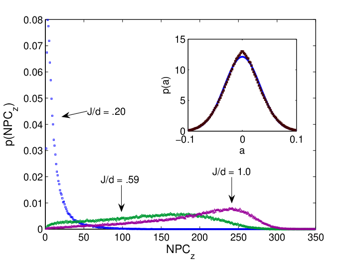
Associated with the transition in level statistics, there is a transition from eigenvectors which are well localized in the eigenbasis of , to eigenvectors which are delocalized and approximately random (Fig. 1). Generally, for fully developed chaos, the eigenvectors achieve a distribution of components uniform over the surface of an -sphere. In systems obeying time-reversal invariance or, more generally as mentioned, an appropriate anti-unitary symmetry [23, 41], this is equivalent to a Gaussian distribution of eigenstate components in the limit of large . However, as seen in Fig. 1, for this model the states for which is near the expected value for random states of [42] have a component distribution which is only approximately Gaussian. Furthermore, there is no regime where most eigenvectors have an consistent with the expected value for random states, although this value does serve as an approximate upper bound on delocalization. At specific values, this model typically exhibits a fairly wide distribution of .
Throughout the localized-to-delocalized transition, we examined the relationship between and local purity for each eigenvector in the subspace. In Fig. 2, is plotted against for each eigenvector using a single random disorder realization and four representative values of . At , is averaged over each eigenvector between integer values of and over 100 disorder realizations, resulting in a smooth curve which closely fits
| (25) |
see inset in Fig. 2. The value is chosen because of the corresponding wide distribution of . Similarly constructed average curves for other values of , however, do not show significant differences.


In spite of qualitative agreement, the averaged relationship between and given in Eq. (25) deviates from the relationship predicted in Eq. (13) under the assumption of Hamming uncorrelation between and . This indicates that the do depend non-trivially on Hamming distance in general. In Fig. 3, is averaged over each eigenvector between integer values of and 100 disorder realizations at . Especially for small , tends to be larger for smaller values of . There is a strong peak in at , and a less pronounced peak in at . All other rise gradually. As approaches the limiting value of , the values of the become closer to each other, and appear in good agreement with the expected value for random states, [43]. and (data not shown) lie close to .
In the perturbative regime, the dependence of on Hamming distance may be understood as a consequence of the two-body form of the interaction. For small , the eigenvectors may be expanded in a perturbation series. Starting with an arbitrary eigenvector of ,
The diagonal contribution may be incorporated into the unperturbed diagonal energies for the current reasoning. Since the Heisenberg interaction only couples eigenstates of which are Hamming distance of away from each other, every state that appears in the first-order sum is a Hamming distance of 2 away from . The states that appear in the second-order sum are Hamming distance 2 or 4 away from . Thus, for an eigenstate in the perturbative regime, all of the first-order products will contribute to . No product larger than second-order will contribute to , and so on. After the breakdown of perturbation theory, the continue to show a dependence on order in perturbation theory for all values of , however, the effect decreases as approaches the random state value of .
An interesting question is the behavior of the relationship between and in the thermodynamic limit where . Because the relationship between local purity and involves averages over all pairs of basis states of fixed Hamming distance, it is reasonable to conjecture that the relationship should become increasingly sharp in this limit, provided that the average value of for fixed order in perturbation theory exists.
6 Conclusion
We have quantified the relationship between delocalization as measured by in a maximal set of mutually unbiased product bases and global entanglement as measured by local purity. In general, the relationship between the two depends on how products of state vector components are correlated with respect to Hamming distance – or a suitable generalization for higher-dimensional subsystems. Under the condition that no such correlation exists, a simple relationship between in each basis and local purity is established. For states with certain physically relevant symmetries, the number of bases may be reduced. In addition, for each state, there always exists a basis in which the local purity is related to in this single basis through correlations with respect to Hamming distance. Such analysis yields an expression for local entanglement, GEloc, as the expectation value of Hamming distance between measurements of two copies of the same pure state in the state-dependent canonical basis where each reduced density matrix is diagonal.
Distributions of random states under which the assumption of uncorrelation is naturally satisfied are also discussed. A simple method to calculate the expected relative purity over an ensemble of pure states invariant under the Haar measure is introduced, and illustrated in several examples. Lastly, the connection between local purity and correlations between products of components is investigated numerically for a disordered Heisenberg spin chain. Because the deviation of the relationship between and from that predicted under the uncorrelation assumption is likely a consequence of the two-body nature of the interaction, a similar relationship is predicted to hold for any disordered qubit system with two-body interactions which has symmetry properties allowing in a single basis to enter the relationship with . For systems without such symmetries, we conjecture that the associated with in the eigenbasis of will still provide the main contribution to , until the eigenvectors are maximally random. Thus, the relationship between and in the eigenbasis of may be generic to all disordered many-body systems.
As a general remark, we also expect the correlation between products of components and Hamming distance to be relevant to other entanglement measures. For instance, the -tangle is written as a sum of products of pairs that are Hamming distance -apart. Thus, we conjecture that this characteristic structure may be important for the study of entanglement properties across a localized-to-delocalized transition and across quantum criticality in many-body systems.
Acknowledgments
L.V. is especially indebted to Howard Barnum and Gerardo Ortiz for continuous exchange and uncountable discussions on the meaning and usefulness of generalized entanglement. The authors also thank Simone Montangero, Lea F. Santos, and Yaakov S. Weinstein for feedback and a critical reading of the manuscript, and Jay Lawrence for discussions on mutually unbiased bases. W.G.B. gratefully acknowledges partial support from Constance and Walter Burke through their Special Projects Fund in Quantum Information Science, and current support from a GAANN Fellowship.
References
References
- [1] Nielsen M A 2002 Sci. Amer. November Issue
- [2] Buhrman H, van Dam W, Hoyer P and Tapp A 1999, Phys. Rev. A60, 2737; Raz R 1999 in Proceedings of the 31st Annual ACM Symposium on Theory of Computing (New York: ACM Press), p. 358
- [3] Jozsa R and Linden N 2003 Proc. R. Soc. London A 459, 2001; Vidal G 2001 Phys. Rev. Lett. 91, 147902
- [4] Osborne T J and Nielsen M A 2002 Phys. Rev. A 66, 032110; Osterloh A, Amico L, Falci G and Fazio R 2002 Nature, 609; Vidal G, Latorre J I, Rico E and Kitaev A 2003 Phys. Rev. Lett. 90, 227902; Roscilde T, Verrucchi P, Fubini A, Haas S and Tognetti V 2005 Phys. Rev. Lett. 93, 147208
- [5] Somma R, Ortiz G, Barnum H, Knill E and Viola L 2004 Phys. Rev. A 70, 042311
- [6] Bandyopadhyay J N and Lakshminarayan A 2002 Phys. Rev. Lett. 89, 060402; Montangero S, Benenti G, Fazio R 2003 Phys. Rev. Lett. 91, 187901; Santos L F, Rigolin G and Escobar C 2004 Phys. Rev. A 69, 042304
- [7] Mejia-Monasterio C, Benenti G, Carlo G G and Casati G 2005 Phys. Rev. A 71 062324
- [8] Scott A J and Caves C M 2003 J. Phys. A. 36, 9553
- [9] Vidal G 2005 arXiv e-print quant-ph/0512165; Porras D, Verstraete F and Cirac J I 2006 Phys. Rev. B 73, 094423
- [10] Barnum H, Knill E, Ortiz G and Viola L 2003 Phys. Rev. A 68, 032308; Barnum H, Knill E, Ortiz G, Somma R and Viola L 2004 Phys. Rev. Lett. 92, 107902
- [11] Montangero S and Viola L 2006 Phys. Rev. A 73 (R)040302
- [12] Weinstein Y S and Viola L 2006 Europhys. Lett. 76, 746
- [13] Somma R, Barnum H, Knill E and Ortiz G 2006 Phys. Rev. Lett. 97, 190501
- [14] Amico L, Fazio R, Osterloh A and Vedral V 2007 Rev. Mod. Phys., forthcoming
- [15] Ortiz G, Somma R, Barnum H, Knill E and Viola L 2004 in: CMT27 (Toulouse) Workshop Proceedings, Vol. 19, Condensed Matter Theories (Nova Science Publisher)
- [16] Viola L, Barnum H, Knill E, Ortiz G and Somma R 2005 Contemp. Math. 381, 117
- [17] Barnum H, Ortiz G, Somma R and Viola L 2005 Int. J. Theor. Phys. 44, 2127
- [18] Viola L and Barnum H 2007 in: Proceedings of the Boston Colloquium for Philosophy of Science on “Foundations of Quantum Information and Entanglement”, forthcoming
- [19] Note that such a projection need not lead to a positive (semidefinite) operator on the full state space. If the identity operators is included in , is positive in the standard multipartite case and positive in general upon restricting its domain to [17, 18]. In practice, since omitting the identity has no effect on the convex structure, traceless distinguished observables are often considered to the purposes of constructing measures of GE.
- [20] Brennen G K 2003 Quantum Inf. Comput. 3, 619
- [21] Meyer D A and Wallach N R 2002 J. Math. Phys. (N.Y.) 43, 4273
- [22] Bengtsson I and Zyczkowski K 2006 Geometry of Quantum States (Cambridge: Cambridge University Press)
- [23] Haake F Quantum Signatures of Chaos 1991 (Berlin: Springer-Verlag)
- [24] Different conventions and terminology are found in the literature. In fact, there are at least three names given to the quantity defined in Eq. (6): In addition to the NPC terminology we follow here (see e.g. V. K. B Kota and R. Sahu, 2001 Phys. Rev. E 64, 016219), NPC is also, as mentioned in the text, referred to as “participation number” (PN) in [7]. Furthermore, the definitions of NPC vs IPR are often interchanged, as in [11]. Adding to the confusion, there is overlap in terminology with a similar measure of mixedness, , which is also sometimes referred to as either IPR or PN, see e.g. [37].
- [25] Lawrence J, Brukner C and Zeilinger A 2002 Phys. Rev. A 65, 032320
- [26] Note that should not be confused with , which involves in this case expectations of arbitrary (non-local) strings of operators on different qubits.
- [27] Li H, Wang X-G, Hu B 2004 J. Phys. A 37, 10665
- [28] Higuchi A and Sudbery A 2000 Phys. Lett. A 273, 213; Carteret H, Higuchi A and Sudbery A 2000 J. Math. Phys. 41, 7932
- [29] Brun T A and Cohen O 2001 Phys. Lett. A 281, 88; Brun T A 2004 Quantum Inf. Comput. 4, 401
- [30] Bandyopadhyay S, Boykin P O, Roychowdhury V and Vatan F 2002 Algorithmica 34, 512
- [31] Mehta M L 1991 Random Matrices (Boston: Academic Press)
- [32] Lubkin E 1978 J. Math. Phys. 19, 1028
- [33] Page D N 1993 Phys. Rev. Lett. 71, 3743; Foong S K and Kanno S 1994 Phys. Rev. Lett. 72, 1148
- [34] Scott A J 2004 Phys. Rev. A 69, 052330
- [35] Hayden P, Leung D W and Winter A 2006 Commun Math. Phys. 265, 95
- [36] Dahlsten O and Plenio M 2005 arXiv e-print quant-ph/0511119
- [37] Facchi P, Florio G and Pascazio S 2006 Phys. Rev. A 74, 042331
- [38] Arecchi F T, Courtens E, Gilmore R and Thomas H 1972 Phys. Rev. A 6, 2211
- [39] Demkowicz-Dobrzanski and Kus M 2004 Phys. Rev. E 70, 066216
- [40] Brown W G, Santos L F, Starling D and Viola L 2007 “Quantum Chaos, Localization, and Entanglement in Disordered Heisenberg Models,” forthcoming
- [41] Avishai Y, Richert J and Berkovits R 2002 Phys. Rev. B 66, 052416
- [42] Strictly speaking, is the expected value of IPR, cf Eq. (22). However, because the distribution of states with values around the expected IPR becomes quickly sharp as increases, we identify .
- [43] This value is obtained by using (where -dependences are implicit throughout). As does not depend on and , and , it follows that . Identifying with and rearranging terms yields the result quoted in the text.