Quantum Dynamics with Bohmian Trajectories
Abstract
We describe the advantages and disadvantages of numerical methods when Bohmian trajectory-grids are used for numerical simulations of quantum dynamics. We focus on the crucial non-crossing property of Bohmian trajectories, which numerically must be paid careful attention to. Failure to do so causes instabilities or leads to false simulations.
1 Introduction
Bohmian Mechanics.
Bohmian Mechanics [4] is a mechanical theory for the motion of particles. We describe the theory in units of mass . Given the Schrödinger wave function of an -particle system, the trajectories of the particles , , are solutions of
| (1) |
with as initial conditions and denoting the complex conjugate of , so that .11 1 Interpreting as inner product, the generalization to spin wave functions is straight forward. We denote the configuration point , where is the gradient with respect to . is the solution of the Schrödinger equation
| (2) |
with the initial condition . Using configuration space language the Bohmian trajectory of an particle system is an integral curve of the following velocity field on configuration space
| (3) |
i.e.
| (4) |
Under general conditions one has global existence and uniqueness of Bohmian
trajectories, i.e. the integral curves do not run into nodes of the wave functions and they cannot cross
[5]. From now on we shall only talk about
the trajectories as integral curves in configuration space. Note
that for one particle the configuration space is equal to physical
space, for more than one particle
this is not the case.
The empirical import of Bohmian Mechanics arises from equivariance of the -measure: One readily sees that by virtue of (3) the continuity equation for the Bohmian flow on configuration space is identically fulfilled by the density , then known as the quantum flux equation,
This means that if
the configuration of particles is distributed according to at time , then the configuration
is distributed according to at any time . Because of
this, Bohmian Mechanics agrees with all predictions made by
orthodox quantum mechanics whenever the latter are unambiguous [2, 3].
Hydrodynamic Formulation of Bohmian Mechanics.
Numerical Integration.
Numerically this set of
equations (5)-(7) can readily be
integrated [6] and offers some advantages over standard
techniques for solving the Schrödinger equation
(2) numerically. The basic idea, due to Wyatt
[6], is that the Bohmian configuration space trajectories
define a co-moving grid (Bohmian grid) in configuration space
which is best adapted for the computation of . If initially
the grid points ( points in ) are
distributed, they will remain distributed for all
times . So the co-moving grid spreads dynamically according to
the spreading of and the grid points will primarily
remain in regions of space where is large while
avoiding regions of nodes or tails of which are
numerically problematic. Therefore Wyatt’s idea is this: Integrate
the equations (5)-(7) simultaneously, i.e. get the best adapted moving grid along with
, instead of integrating the Schrödinger equation on some
fixed or otherwise determined grid. This is why the algorithm is
particularly interesting for long-time simulations which usually
demand huge computational effort on fixed grids. Therefore if one
aims at the relevant parts of the wave function (where
probabilities are high) one can use a fixed number of
distributed Bohmian grid points in , so
that the Bohmian grid simulation scales with the number of
particles [6] while conventional grid methods mostly
scale exponentially with . We say more in section 3
on how to distribute grid points in a manner.
In order to perform the numerical integration of the set of differential equations (5)-(7) we follow the straight-forward method described in [6]. The only crucial part in this is computing the derivatives involved in the set of differential equations. There are several techniques known and [6] gives a comprehensive overview. Among them one technique called least square fitting is commonly used. In this letter we argue that this method is inappropriate for integrating (5)-(7) for general initial conditions and potentials. Bad situations arise whenever Bohmian trajectories move towards each other, because least square fitting will allow crossings of the simulated trajectories which are not allowed for Bohmian trajectories. Once a crossing is encountered in a numerical simulation further computation can be aborted because this numerical wave function would differ immensely from the solution of the Schrödinger equation (2). This will happen generically, i.e. for non-gaussian wave functions. To illustrate our argument we shall present a typical numerical example in one dimension with one particle. Therefore in what follows and the trajectories which we shall consider (making up the grid) are the possible trajectories of this one particle only.
2 Least Square versus Polynomial Fitting
In order to compute the derivatives encountered in (5)-(7) we only consider two different types of fitting, the least square fitting and the polynomial fitting. Most other fitting algorithms are descendants of one or the other. Both provide an algorithm for finding e.g. a polynomial22 2 Or more general an element of a dimensional vector space of functions. The coefficients of the design matrix determine which basis functions are used. of degree, say , which is in some sense to be specified close to a given function known only on a set of, say , pairwise distinct data points, , as subset of the graph of . The derivative can then be computed from the fitting polynomial by algebraic means. Let for the further discussion
Using this notation the problem of finding a fitting polynomial to on the basis of pairwise distinct data points of the graph of reduces to finding the coefficients of the vector obeying the equation
such that the error term is in some sense small. Here the dot denotes matrix multiplication. The fitting polynomial is given by .
Polynomial Fitting.
For the case we can choose the error term to be identical zero since is an invertible square matrix and can be straight-forwardly computed.
Least Square Fitting.
For arbitrary there is no unique solution anymore and one needs a new criterion for finding a unique vector . The algorithm of least square fitting uses therefore the minimum value of the accumulated error where specifies a weight dependent on the distance between the -th data point and some point where the fitting polynomial shall be evaluated. The vector can now be determined by minimizing as a function of by solving
Note that for and any non-zero weight the algorithm of least square fitting produces the same as the polynomial fitting would do since for the determined by polynomial fitting the non-negative function is zero and thus naturally minimizes the error term.
Why Least Square Fitting is inappropriate for Bohmian Grids.
The algorithm of least square fitting is well known for its tendency to stabilize numerical simulations by averaging out numerical errors. But exactly this averaging makes it hard to keep the grid points from crossing each other. In order to understand what happens during a numerical simulation recall the form of the equations of motion (5)-(7) which have to be integrated step by step. The change in time of the phase is determined by three terms in equation of (7). The first two terms form the classical Lagrangian and depend on the current velocities of the grid points and on the potential . The third term is the so-called quantum potential and depends only on and its second derivative. The quantum potential is what prevents Bohmian trajectories from crossing each other. It therefore needs special attention during the numerical integration. Now imagine initial conditions such that two grid points approach each other. An increase of the density of the grid points in a region where the two grid points move towards each other will cause a small bump in . By small bump we mean a bump of the wave function shape on a microscopic scale, i.e. a scale defined by few grid points. Such a small bump of may have large derivatives changing the quantum potential in (7). Thus, it is absolutely vital for a numerical simulation to implement a fitting algorithm that reconstructs not only , respectively , in an accurate way but also its second derivative. The tendency of the least square fitting algorithm is to average out those small bumps in , respectively . Hence, the simulation is blind to recognize grid points moving towards each other and hence does not prevent a crossing of these trajectories.
Note that since the averaging occurs on a microscopic scale, situations in which grid points move only very slowly or do generically not move towards each other33 3 For example a free Gaussian wave packet or one approaching a potential creating only soft reflections. are often numerically doable with least square fitting. On the other hand numerical simulations with least square fitting in general situations like the one discussed above are bound to break down as soon as two grid points get too close to each other.
Why Polynomial Fitting is more appropriate for Bohmian Grids.
We stressed above that small bumps may exponentiate numerical instability. A good numerical method must take note of the small bumps and must prevent their increase. Such a numerical method is provided by polynomial fitting, since there the polynomials go through all grid points. Therefore polynomial fitting recognizes the bumps of and/or and hence the resulting quantum potential recognizes the approaching grid points. Now recall the physics of the Bohmian evolution, which as we stressed in the introduction prevents trajectories from crossing each other. Therefore we expect that this method is self-correcting and hence stabilizing.
The Boundary Problem.
It has to be remarked that polynomial fitting creates a more severe problem at the boundary of the supporting grid than least square fitting. This problem is of conceptual kind since at the boundary there is a generic lack of knowledge of how the derivatives of or behave, see figure 1.
 |
 |
 |
 |
We describe briefly how this conceptual problem can cause severe numerical instability. For this suppose that only the last grid point in the upper left plot of figure 1 is lifted a little bit upwards by e.g. some numerical error. Then the resulting quantum potential will cause the last grid point to move towards the second last one. This increases the density of grid points and thus again increases in the next step such that this effect is self-amplifying (in fact growing super exponentially) and will effect the whole wave function quickly.
At the boundary the good property of polynomial fitting, namely to recognize all small bumps works against Bohmian grids techniques. In contrary least square fitting simply averages these small numerical errors out, see lower right plot in figure 1. The conceptual boundary problem, however, remains and will show up eventually also with least square fitting.
The Numerical Simulation.
To demonstrate our argument we shall now give a numerical example for one particle in one dimension. We remark as mentioned earlier that Gaussian wave packets are unfit for probing the quality of the numerical simulations. Therefore we take as initial conditions two superposed free Gaussian wave packets with a small displacement together with a velocity field identically to zero and focus the attention on the region where their tails meet, i.e. where the Bohmian trajectories will move towards each other according to the spreading of the wave packets, see figure 2. The physical units given in the figures and the following discussion refer to a wave packet on a length scale of and a Bohmian particle with the mass of an electron.
 |
 |
The numerical simulation is implemented as in [6] with minor changes. It is written in MATLAB using IEEE Standard 754 double precision. In order to ease the boundary problem we use a very strong least square fitting at the boundary. Note that this only eases the boundary problem and is by no means a proper cure. In between the boundary, however, the number of data points for the fitting algorithm and the degree of the fitting polynomial can be chosen in each run. In this way it is possible to have either polynomial fitting or least square fitting in between the boundary. The simulation is run twice. First with the polynomial fitting and then with the least square fitting algorithm in between the boundaries.
We take basis functions for the fitting polynomial in both cases. Note that the choice should at least be greater or equal to in order to have enough information about the third derivative of the fitting polynomial. In the first run with polynomial fitting the number of grid points used for fitting is and in the second run for the least square fitting we choose which induces a mild least square behavior. For the numerical integration we have used a time step of with the total number of grid points supporting the initial wave function. Please find the source code of our numerical simulation at the end of this letter.
Results.
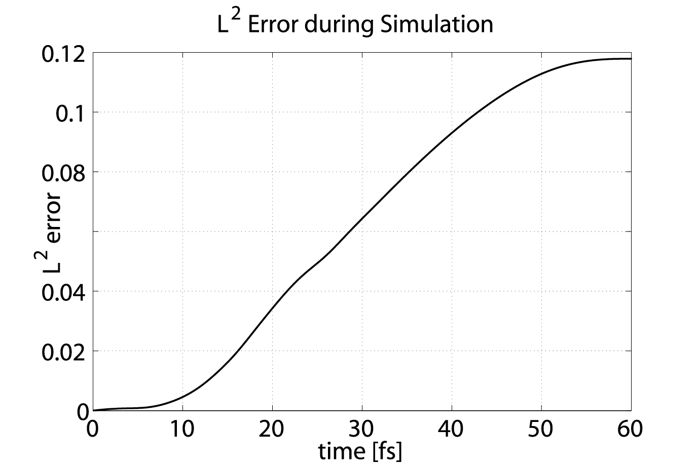
The first run with polynomial fitting yields accurate results and does not allow for trajectory crossing way beyond integration steps, i.e. , see figures 3 and 4. The second run with least square fitting reports a crossing of trajectories already after 430 integration steps, i.e. , and aborts, see figures 5 and 6. The numerical instability can already be observed earlier, see left-hand side of figure 5. An adjustment of the time step of the numerical integration does not lead to better results in the second run. The crossing of the trajectories of course occurs exactly in the region were the grid points move fastest towards each other. Referring to the discussion before, the small bumps in created by the increase of the grid point density in this region is not seen by the least square algorithm and thus not seen by the numerical integration of equations (5)-(7), compare figure 3 and 5. The approaching grid points are not decelerated by the quantum potential and finally cross each other, see figure 5, while in the first run they begin to decelerate and turn to the opposite direction during the time between to , see figure 3. To visualize how the two algorithms ”see” and the velocity field during numerical integration these entities have been plotted in figures 3 and 5 by merging all fitting polynomials in the neighborhood of every grid point together (from halfway to the left neighboring grid point to halfway to the right neighboring grid point). In figure 5 one clearly observes the failure of the least square fitting algorithm to see the small bumps in .
Note that in some special situations in which the time step of the numerical integration is chosen to be large, polynomial fitting may lead to trajectory crossing as well. This may happen when the number of time steps in which the simulation has to decelerate two fast approaching grid points is not sufficient. This effect is entirely due to the fact that numerical integration coarse grains the time. The choice of a smaller time step for the simulation will always cure the problem as long as other numerical errors do not accumulate too much.
The relevant measure of quality of the numerical simulation is naturally the distance between the simulated wavefunction and the analytic solution of the Schrödinger equation , i.e. , and is spelled out on the left-hand side of the figures 4 and 6 for both runs.
 |
 |
 |
 |
 |
 |
 |
 |
 |
 |
 |
 |
3 Using as Initial Distribution.
As discussed in the introduction, if the grid point are distributed according to , they will remain so for all times. Doing so will bring two advantages but comes at the price of a more severe conceptual boundary problem as discussed in the last section. The first advantage is that this Bohmian grid avoids regions where is very small and thus where the computation of the quantum potential becomes numerically tricky. The second advantage is that now the system is over-determined and the actual density of grid points must coincide with for all times. This could be used as an on the fly check whether the grid points behave like Bohmian trajectories or not. If not the numerical integration does not give a good approximation to the solution of (5)-(7). It could also be considered to stabilize the numerical simulation with a feedback mechanism balancing and the distribution of the particle positions which may correct numerical errors of one or the other on the fly.
One way of choosing distributed initial positions for the grid points for for some large number is the following. Choose in such a way that
| (8) |
This formula can be used to compute the grid points iteratively44 4 This procedure of setting the initial grid points might run into a node of . In that case one should simply start with a slightly shifted initial grid point starting with some grid point near the maximum of . Another way is to simulate distributed random variables by the commonly used techniques. Here, however, it has to be taken care that the randomly chosen do not lie too close together. If they do, either some of them must be deleted or the time step of the numerical integration must be adjusted carefully. A rule of thumb is that the distance of approaching grid points divided by their relative velocity has to be a lot smaller than the chosen time step.
4 Conclusion
Using polynomial fitting instead of least square fitting in between the boundary increases the stability of the numerical integration immensely. This is due to the fact that polynomial fitting in contrary to least square fitting does not average over the microscopic structure of the function to fit and therefore reconstructs needed derivatives more accurately. The discussed boundary problem arises more severely for polynomial fitting because of this fact. However, this problem is generic to the numerical integration considered here and also occurs using least square fitting but in a milder way. We suggest that the smoothness of the decay of the wave function near the boundary should be the guide for solving this problem which requires a detailed study. Furthermore, we have discussed that the Bohmian grid is best adapted to the problem of numerical integration of (5)-(7) because the grid points naturally avoid regions where becomes very small.
5 Acknowledgment
We thank Bob Wyatt for acquainting us with the Bohmian grid methods in theoretical chemistry. We further thank in alphabetical order: Lara Hernando, Salvador Miret-Artes, Angel Sanz, Clemens Woywod for discussions. This work was partly supported by DFG. D.-A. Deckert would like to cordially thank R.-R. Deckert and W.E. Göhde-Deckert for funding and support.
References
- [1]
D.-A. Deckert, D. Dürr, P. Pickl.
Quantum Dynamics with Bohmian Trajectories.
arXiv:quant-ph/0701190, 2007. - [2] D. Dürr, S. Goldstein, and N. Zanghì. Quantum Equilibrium and the Origin of Absolute Uncertainty. Journal of Statistical Physics, 67:843–907, 1992.
- [3] D. Dürr, S. Goldstein, and N. Zanghì. Quantum equilibrium and the role of operators as observables in quantum theory. Journal of Statistical Physics, 116:959–1055, 2004.
- [4] S. Goldstein. Bohmian mechanics. Contribution to Stanford Encyclopedia of Philosophy, ed. by E.N. Zalta, http://plato.stanford.edu/entries/qm-bohm/, 2001.
- [5] S. Teufel and R. Tumulka. Simple proof for global existence of bohmian trajectories. Commun. Math. Phys., (258):349–365, 2005.
- [6] R.E. Wyatt. Quantum Dynamics with Trajectories. Springer, 2005.
SOURCE CODE OF THE NUMERICAL SIMULATION:

%% definition of constants and rendering of initial value

%CONSTANTS & SYMPBOLS*****************************************************

fovx            = 8;        %field of view on the real line [-fovx, fovx].
numParticles    = 51;       %number of Bohmian particles.
dt              = 10^-2;    %time step for numerical integration.
numSteps        = 6000;     %number of iterations of the numerical
                            %integration.
stencil         = 3;        %number of points left and right w.r.t. some
                            %point for fitting 0.5*log(rho).
degree          = 6;        %degree of polynomial for fitting
                            %please note: stencil=degree/2 means a
                            %precise polynomial fit of ’degree’ degree
                            %while stencil>degree/2 means a least square
                            %fit with a polynomial of degree ’degree’.
s_stencil       = 3;        %log(sqrt(rho)) number of points left and
                            %right w.r.t. some point for fitting the
                            %phase.
s_degree        = 6;        %degree of polynomial for fitting the phase.
                            %the above note hols for the phase.

sym_x  = sym(’sym_x’,’real’);   %dummy symbol for symbolic math

%FUNCTIONS****************************************************************

%-------------------------------------------------------------------------
% Analytic solution of an initial gaussian evolved according to the free
% Schroedinger equation.
% INPUT : t=time of evolution, x=position, sigma=initial width of the
%         gaussian
% OUTPUT: complex value of the wavefunction
gauss  = @(t, x, sigma) (sigma/(pi*(sigma+i*t)^2))...
                        .^(1/4).*exp(-x.^2/(2*(sigma^2+t^2))*(sigma-i*t));

%-------------------------------------------------------------------------
% psi=analytic solution of a superposition of initial gaussians evolved
% according to the free Schroedinger equation.
% rho,S,vel=|psi|^2, the phase, the velocity field of psi
% INPUT : t=time of evolution, x=position
% OUTPUT: real resp. complex function value
psi    = @(t, x) 1/sqrt(2)*(gauss(t,x-3,4)+gauss(t,x+3,4));
rho    = @(t, x) psi(t,x).*conj(psi(t,x));
S      = @(t, x) imag(log(psi(t,x)./abs(psi(t,x))));
vel    = @(t, x) imag(subs(diff(psi(t,sym_x),sym_x)...
                 ./psi(t,sym_x),sym_x,x));

%INITIAL DATA-------------------------------------------------------------

clear x;                                %initial distribution of the
                                        %Bohmian particles
x = [-fovx:(2*fovx/numParticles):fovx]; %generate a uniform distribution

%plot the initial data: blue=initial rho and green=initial veleocity field
plot(x, vel(0,x), ’g’, x, rho(0,x), ’b.-’);
axis([-fovx fovx -1 1]);
grid on;

%% bohmian propagation

warning off;

%initialize the array that keeps track of the (x,0.5*log(rho),S,time)
%data history.
history = [{x vel(0,x) 0.5*log(rho(0,x)) S(0,x) 0}];

%loop over the numer of time steps of numerical integration
for (step = 1:numSteps)

    xlen = length(history{step,1});

    x_list          = history{step,1};
    vel_list        = history{step,2};
    logsqrtRho_list = history{step,3};
    s_list          = history{step,4};

    %first loop over the all Bohmian particles updating the
    %x_list and s_list
    for (c = 1:xlen)
        %find stencil points for logsqrtRho
        left_point  = c - stencil;
        right_point = c + stencil;
        deg = degree;
        if (left_point < 1)
            left_point  = 1;
            right_point = stencil*2+1 + round(numParticles/7);
            %decrease degree at the boundary as dodgy fix to avoid
            %bouadary problems
            deg = 2;
        elseif (right_point > xlen)
            left_point  = xlen - (2*stencil+1) - round(numParticles/7);
            right_point = xlen;
            %decrease degree at the boundary as dodgy fix to avoid
            %bouadary problems
            deg = 2;
        end
        %fit logsqrtRho_list
        fitdata_x = history{step,1}(left_point:right_point);
        fitdata_y = history{step,3}(left_point:right_point);
        logsqrtRho_fit = polyfit(fitdata_x, fitdata_y, deg);
        %compute derivatives
        d_logsqrtRho_fit = polyder(logsqrtRho_fit);
        dd_logsqrtRho_fit = polyder(d_logsqrtRho_fit);
        %compute quantum potential
        Q = -1/2*(polyval(dd_logsqrtRho_fit,x_list(c)) + ...
            polyval(d_logsqrtRho_fit,x_list(c)).^2);
        %update phase: S(t+dt)=S(t)+dt(1/2v(t)^2-Q(t))
        s_list(c) = s_list(c) + (1/2*vel_list(c).^2 - Q)*dt;
        %update position: r(t+dt)=r(t)+v(t)*dt
        x_list(c) = x_list(c) + vel_list(c)*dt;
    end

    %second loop over the all Bohmian particles updating
    %the vel_list and logsqrtRho_list
    for (c = 1:xlen)
        %find stecil points for S
        s_left_point  = c-s_stencil;
        s_right_point = c+s_stencil;
        deg = s_degree;
        if (s_left_point < 1)
            s_left_point  = 1;
            s_right_point = s_stencil*2+1 + round(numParticles/7);
            %decrease degree at the boundary as dodgy fix to avoid
            %bouadary problems
            deg = 2;
        elseif (s_right_point > xlen)
            s_left_point  = xlen - (2*s_stencil+1) - round(numParticles/7);
            s_right_point = xlen;
            %decrease degree at the boundary as dodgy fix to avoid
            %bouadary problems
            deg = 2;
        end
        %fit s_list
        fitdata_x = x_list(s_left_point:s_right_point);
        fitdata_y = s_list(s_left_point:s_right_point);
        s_fit = polyfit(fitdata_x, fitdata_y, deg);
        %compute derivatives
        d_s_fit = polyder(s_fit);
        dd_s_fit = polyder(d_s_fit);
        %v(t+dt) = S’(t+dt)
        vel_list(c) = polyval(d_s_fit,x_list(c));
        %R(t+dt) = R(t)*exp(-1/2 S’’(t+dt)*dt)
        logsqrtRho_list(c) = logsqrtRho_list(c)-...
                             1/2*polyval(dd_s_fit,x_list(c))*dt;
    end

    %compile the tuple (x,vel,0.5*log(rho),time)
    newSnapshot = [{x_list vel_list ...
                    logsqrtRho_list s_list history{step,5}+dt}];
    %and save the snapshot
    history = [history; newSnapshot];

    %compute minimal distance of the Bohmian particles
    dxmin  = min(x_list(2:length(x_list))-x_list(1:length(x_list)-1));
    if (dxmin <= 0)
        sprintf(’TRAJECTORY CROSSING OCCURED AT TIME: %f’,...
                history{step,5}+dt)
        break;
    end

    if (step == 1 | mod(step/numSteps*100,10) == 0)
        %plot integrated velocity field
        plot(x_list(1):0.1:x_list(xlen),vel(history{step,5}+dt,...
             x_list(1):0.1:x_list(xlen)),’r’,x_list,vel_list,’b.’);
        axis([-25 25 -5 5]);
        grid on;
        sprintf(’Progress: %.1f%%, timestep: %f fs, min deltax: %f’,...
                step/numSteps*100, history{step,5}+dt, dxmin)
        pause(0.1);
    end
end

%% render rho movie (red is the analytic solution)
frame = 1;
clear(’rhoMov’);
for step=1:10:length(history)
    plot(-25:0.1:25,rho(history{step,5},-25:0.1:25),’r’,...
         history{step,1},exp(history{step,3}*2),’b.’,...
         history{step,1},0,’b*’);
    axis([-25 25 0 0.3]);
    grid on;
    pause(0.05);
    rhoMov(frame) = getframe;
    frame = frame + 1;
end

%% render vel movie (red is the analytic solution)
frame = 1;
clear(’velMov’);
for step=1:10:length(history)
    plot(-20:0.1:20,vel(history{step,5},-20:0.1:20),’r’,...
         history{step,1},history{step,2},’b.’);
    axis([-25 25 -5 5]);
    grid on;
    velMov(frame) = getframe;
    frame = frame + 1;
end

%% render velocity field seen by the above algorithm

diagAxis = [-10 10 -1 1];

%loop over the number of time steps of numerical integration
for (step = 1:length(history))

    xlen = length(history{step,1});

    xvals = [];
    yvals = [];

    %loop over all particles
    for (c = 1:xlen)
        %find stecil points for S
        s_left_point  = c-s_stencil;
        s_right_point = c+s_stencil;
        deg = s_degree;
        if (s_left_point < 1)
            s_left_point  = 1;
            s_right_point = s_stencil*2+1 + round(numParticles/7);
            %decrease degree at the boundary as dodgy fix to avoid
            %bouadary problems
            deg = 2;
        elseif (s_right_point > xlen)
            s_left_point  = xlen - (2*s_stencil+1) - round(numParticles/7);
            s_right_point = xlen;
            %decrease degree at the boundary as dodgy fix to avoid
            %bouadary problems
            deg = 2;
        end
        %fit s_list
        fitdata_x = history{step,1}(s_left_point:s_right_point);
        fitdata_y = history{step,4}(s_left_point:s_right_point);
        s_fit = polyfit(fitdata_x, fitdata_y, deg);
        %compute velocity
        d_s_fit = polyder(s_fit);
        %compute graph

        if (c == 1)
            x1 = history{step,1}(c)-1;
            x2 = history{step,1}(c) ...
                 + (history{step,1}(c+1)-history{step,1}(c))/2;
        elseif (c == xlen)
            x1 = history{step,1}(c-1) ...
                 + (history{step,1}(c)-history{step,1}(c-1))/2;
            x2 = history{step,1}(c)+1;
        else
            x1 = history{step,1}(c-1) ...
                 + (history{step,1}(c)-history{step,1}(c-1))/2;
            x2 = history{step,1}(c) ...
                 + (history{step,1}(c+1)-history{step,1}(c))/2;
        end

        xvals = [ xvals x1:((x2-x1)/100):x2 ];
        yvals = [ yvals polyval(d_s_fit,x1:((x2-x1)/100):x2)];
    end

    plot(xvals,vel(history{step,5},xvals),’r’,xvals,yvals,’b’,...
         history{step,1},history{step,2},’b.’);
    axis(diagAxis);
    grid on;
    pause(0.1);
end

%% render rho field seen by the above algorithm

diagAxis = [-30 30 0 0.145];

%loop over the number of time steps of numerical integration
for (step = 1:length(history))

    xlen = length(history{step,1});

    xvals = [];
    yvals = [];

    %loop over all particles
    for (c = 1:xlen)
        %find stencil points for logsqrtRho
        left_point  = c - stencil;
        right_point = c + stencil;
        deg = degree;
        if (left_point < 1)
            left_point  = 1;
            right_point = stencil*2+1 + round(numParticles/7);
            %decrease degree at the boundary as dodgy fix to avoid
            %bouadary problems
            deg = 2;
        elseif (right_point > xlen)
            left_point  = xlen - (2*stencil+1) - round(numParticles/7);
            right_point = xlen;
            %decrease degree at the boundary as dodgy fix to avoid
            %bouadary problems
            deg = 2;
        end
        %fit logsqrtRho_list
        fitdata_x = history{step,1}(left_point:right_point);
        fitdata_y = history{step,3}(left_point:right_point);
        logsqrtRho_fit = polyfit(fitdata_x, fitdata_y, deg);
        %compute derivatives
        d_logsqrtRho_fit = polyder(logsqrtRho_fit);
        dd_logsqrtRho_fit = polyder(d_logsqrtRho_fit);
        %compute quantum potential
        Q = -1/2*(polyval(dd_logsqrtRho_fit,x_list(c)) + ...
            polyval(d_logsqrtRho_fit,x_list(c)).^2);
        %compute graph

        if (c == 1)
            x1 = history{step,1}(c)-1;
            x2 = history{step,1}(c) ...
                 + (history{step,1}(c+1)-history{step,1}(c))/2;
        elseif (c == xlen)
            x1 = history{step,1}(c-1) ...
                 + (history{step,1}(c)-history{step,1}(c-1))/2;
            x2 = history{step,1}(c)+1;
        else
            x1 = history{step,1}(c-1) ...
                 + (history{step,1}(c)-history{step,1}(c-1))/2;
            x2 = history{step,1}(c) ...
                 + (history{step,1}(c+1)-history{step,1}(c))/2;
        end

        xvals = [ xvals x1:0.05:x2 ];
        yvals = [ yvals polyval(logsqrtRho_fit,x1:0.05:x2)];
    end

    plot(xvals,rho(history{step,5},xvals),’r’,xvals,exp(2*yvals),’b’,...
         history{step,1},exp(2*history{step,3}),’b.’);
    axis(diagAxis);
    grid on;
    pause(0.1);
end

%% render trajectories

diagAxis = [-12 12 0 length(history)*dt];
hold off;
grid off;

%loop over the grid points
for (j = 1:numParticles)
    xvals = [];
    yvals = [];
    for (step = 1:length(history))
        xvals = [xvals; history{step,1}(j)];
        yvals = [yvals; history{step,5}];
    end

    plot(xvals,yvals,’k-’);
    axis(diagAxis);
    hold on;
    pause(0.1);
end
hold off;

%% render L^2 error
psi2error = [];
for (step = 1:length(history))
    xdiff  = [];
    ydiff2 = [];
    for (j = 1:numParticles-1)
        xdiff = [xdiff; history{step,1}(j+1)-history{step,1}(j)];
        ydiff2 = [ydiff2; abs(exp(complex(0,history{step,4}(j+1)))...
                              .*exp(history{step,3}(j+1))...
                              - psi((step-1)*dt,history{step,1}(j+1)))^2];
    end
    psi2error = [psi2error; sqrt(sum(xdiff.*ydiff2))];
end
plot((1:length(history))*dt,psi2error,’k’);