Trapping of light pulses in ensembles of stationary $\Lambda$ atoms

Kristian Rymann Hansen Affiliation: Lundbeck Foundation Theoretical Center for Quantum System Research, Department of Physics and Astronomy, University of Aarhus, DK-8000 Århus C, Denmark Klaus Mølmer Affiliation: Lundbeck Foundation Theoretical Center for Quantum System Research, Department of Physics and Astronomy, University of Aarhus, DK-8000 Århus C, Denmark

Abstract

We present a detailed theoretical description of the generation of stationary light pulses by standing wave electromagnetically induced transparency in media comprised of stationary atoms. We show that, contrary to thermal gas media, the achievable storage times are limited only by the ground state dephasing rate of the atoms, making such media ideally suited for nonlinear optical interactions between stored pulses. Furthermore, we find significant quantitative and qualitative differences between the two types of media, which are important for quantum information processing schemes involving stationary light pulses.

pacs

42.50.Gy, 32.80.Qk

I Introduction

The coherent transfer of quantum states between light and atoms has been the subject of much research, both experimentally and theoretically, motivated by potential applications in quantum computing, quantum cryptography and teleportation. While the transfer of quantum states from light to a single atom can in principle be achieved by cavity QED techniques Cirac, the required strong-coupling regime is experimentally very difficult to reach. To overcome this difficulty the use of atomic ensembles, rather than single atoms, has been proposed Kozhekin; Fleischhauer1; Kuzmich; Sherson and implemented for storage of classical light pulses Liu; Phillips, and recently storage of non-classical pulses has been demonstrated Julsgaard; Eisaman. One such light storage scheme is based on electromagnetically induced transparency (EIT) Harris in ensembles of $\Lambda$ -type atoms Fleischhauer1. While the storage and retrieval of light pulses with this scheme has been demonstrated utilizing many different types of atomic ensembles, including Bose-Einstein condensates Liu and thermal gasses Phillips as well as solid state media Turukhin; Longdell, the non-trivial manipulation of, and interaction between, stored pulses is hampered by the inherent trade-off between storage time and field amplitude. A step towards overcoming this problem was taken with the suggestion of using standing wave fields to create a periodic modulation of either the dispersive Andre1 or the absorptive Bajcsy properties of the medium, inducing a photonic bandgap Yariv and creating a stationary light pulse. Schemes to implement a controlled phase gate using these techniques have been proposed using either the dispersive Friedler or the absorptive Andre2 grating technique, but both are still hampered by a trade-off between storage time and field amplitude. For the latter case, only thermal gas media have been considered, and a detailed theoretical treatment of this case is given in Zimmer. This theory, however, does not apply to media comprised of stationary atoms such as ultra cold gasses or solid state media Hansen. In this article we present a detailed theoretical treatment of the creation of stationary light pulses by the absorptive grating technique for media comprised of stationary atoms. We find that the loss of excitations inherent to the thermal gas case is absent for stationary atoms, making such media ideally suited for the kind of non-linear optical interactions envisaged in Andre2. Furthermore we find interesting quantitative and qualitative differences between the thermal gas and ultra cold gas cases when quasi-standing wave coupling fields are considered. These differences are important for the proposed controlled phase gate scheme Andre2 in stationary atom media.

In Sec. II we present a detailed account of our theory of stationary light pulses in media comprised of stationary atoms and compare the results to the thermal gas case. The theory is complemented in Sec. III by a calculation of non-adiabatic corrections. A summary of our results is provided in Sec. IV. Appendix A contains a brief review of the theory of stationary light pulses in thermal gas media Zimmer, reformulated in terms of polariton fields, used for comparison with the stationary atom case.

II Standing wave polaritons in ensembles of stationary atoms

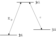
We consider an ensemble of $N$ non-moving $\Lambda$ atoms interacting with probe and coupling lasers propagating parallel to the $z$ axis. The two lower states $|b\rangle$ and $|c\rangle$ of the atoms (see Fig. ) are assumed to be nearly degenerate, such that the magnitude of the wave vectors of the probe and coupling lasers can be considered identical $(k_{p}\simeq k_{c}=k)$ .

Refer to caption — Figure 1: The 3-level $\Lambda$ atom. The quantized probe field couples the ground state $|b\rangle$ to the excited state $|a\rangle$ , while the classical coupling field couples the metastable state $|c\rangle$ to $|a\rangle$ .

The Hamiltonian for the $N$ atom problem is

\hat{H}=\hat{H}_{F}+\sum_{j=1}^{N}\left(\hat{H}_{A}^{j}+\hat{H}_{L}^{j}+\hat{H}_{V}^{j}\right)

(1)

where $\hat{H}_{F}$ and $\hat{H}_{A}$ describe the free electromagnetic field and the atoms, $\hat{H}_{L}$ describes the interaction of the atoms with the probe and coupling fields, and $\hat{H}_{V}$ describes the interaction with the vacuum field modes. The individual terms are given by


$\displaystyle\hat{H}_{F}$	$\displaystyle=\sum_{m}\hbar\omega_{m}\hat{a}_{m}^{\dagger}\hat{a}_{m}$	(2a)
$\displaystyle\hat{H}_{A}^{j}$	$\displaystyle=\hbar\omega_{cb}\hat{\sigma}_{cc}^{j}+\hbar\omega_{ab}\hat{\sigma}_{aa}^{j}$	(2b)
$\displaystyle\hat{H}_{L}^{j}$	$\displaystyle=-\bigl(\hat{\mathbf{E}}_{p}+\hat{\mathbf{E}}_{c}\bigr)\cdot\bigl(\mathbf{d}_{ba}\hat{\sigma}_{ba}^{j}+\mathbf{d}_{ca}\hat{\sigma}_{ca}^{j}+\mathrm{h.a.}\bigr)$	(2c)
$\displaystyle\hat{H}_{V}^{j}$	$\displaystyle=-\hat{\mathbf{E}}_{V}\cdot\bigl(\mathbf{d}_{ba}\hat{\sigma}_{ba}^{j}+\mathbf{d}_{ca}\hat{\sigma}_{ca}^{j}+\mathrm{h.a.}\bigr)$	(2d)

We introduce slowly varying field operators for the electromagnetic field. Since we are allowing for standing wave fields, we write the field operator as a superposition of two traveling wave fields propagating in opposite directions

\hat{\mathbf{E}}_{p,c}(z,t)=\sqrt{\frac{\hbar\omega_{p,c}}{2\varepsilon_{0}V}}\mathbf{e}_{p,c}E_{p,c}(z,t)e^{-i\omega_{p,c}t}+\text{h.c.}

(3)

where the operators $E_{p,c}$ are given by

E_{p,c}(z,t)=E_{p,c}^{+}(z,t)e^{ikz}+E_{p,c}^{-}(z,t)e^{-ikz}.

(4)

The field operators $E_{p,c}^{\pm}$ are the slowly varying field operators for the forward and backward propagating components of the probe and coupling fields with carrier frequencies $\omega_{p,c}$ , and $\mathbf{e}_{p,c}$ are the respective polarization vectors.

We define continuum atomic operators $\hat{\sigma}_{\mu\nu}$ by summing over the individual atoms in a small volume $V$ , and introduce slowly varying atomic operators $\sigma_{\mu\nu}$ defined by


$\displaystyle\hat{\sigma}_{ba}$	$\displaystyle=\sigma_{ba}e^{-i\omega_{p}t}$	(5a)
$\displaystyle\hat{\sigma}_{ca}$	$\displaystyle=\sigma_{ca}e^{-i\omega_{c}t}$	(5b)
$\displaystyle\hat{\sigma}_{bc}$	$\displaystyle=\sigma_{bc}e^{-i\left(\omega_{p}-\omega_{c}\right)t}.$	(5c)

Notice that the operators defined by (5) are slowly varying in time, but not in space.

The Heisenberg-Langevin equations for these operators in the rotating wave approximation are


$\displaystyle\dot{\sigma}_{aa}$	$\displaystyle=-i\bigl(g_{p}E_{p}^{\dagger}\sigma_{ba}+\Omega_{c}^{*}\sigma_{ca}-\mathrm{h.a.}\bigr)-\gamma\sigma_{aa}+F_{aa}$	(6a)
$\displaystyle\dot{\sigma}_{bb}$	$\displaystyle=i\bigl(g_{p}E_{p}^{\dagger}\sigma_{ba}-\mathrm{h.a.}\bigr)+\gamma_{b}\sigma_{aa}+F_{bb}$	(6b)
$\displaystyle\dot{\sigma}_{cc}$	$\displaystyle=i\bigl(\Omega_{c}^{*}\sigma_{ca}-\mathrm{h.a.}\bigr)+\gamma_{c}\sigma_{aa}+F_{cc}$	(6c)
$\displaystyle\dot{\sigma}_{ba}$	$\displaystyle=i\bigl(g_{p}E_{p}(\sigma_{bb}-\sigma_{aa})+\Omega_{c}\sigma_{bc}\bigr)-\Gamma_{ba}\sigma_{ba}+F_{ba}$	(6d)
$\displaystyle\dot{\sigma}_{ca}$	$\displaystyle=i\bigl(\Omega_{c}(\sigma_{cc}-\sigma_{aa})+g_{p}E_{p}\sigma_{bc}^{\dagger}\bigr)-\Gamma_{ca}\sigma_{ca}+F_{ca}$	(6e)
$\displaystyle\dot{\sigma}_{bc}$	$\displaystyle=i\bigl(\Omega_{c}^{*}\sigma_{ba}-g_{p}E_{p}\sigma_{ca}^{\dagger}\bigr)-\Gamma_{bc}\sigma_{bc}+F_{bc}$	(6f)

where $\gamma=\gamma_{b}+\gamma_{c}$ is the decay rate of the excited state $|a\rangle$ into the two lower states. The complex decay rates $\Gamma_{\mu\nu}$ are given by

$\displaystyle\Gamma_{ba}$	$\displaystyle=\gamma_{ba}-i\delta_{p},$	(7)
$\displaystyle\Gamma_{ca}$	$\displaystyle=\gamma_{ca}-i\delta_{c},$	(8)
$\displaystyle\Gamma_{bc}$	$\displaystyle=\gamma_{bc}-i\Delta,$	(9)

where $\gamma_{\mu\nu}$ are the dephasing rates of the respective coherences, $\delta_{p,c}$ are the one-photon detunings of the probe and coupling lasers, respectively, and $\Delta$ is the two-photon detuning. We have also assumed that the coupling field can be treated as a classical field with Rabi frequency $\Omega_{c}$ given by

\Omega_{c}(z,t)=\Omega_{c}^{+}(z,t)e^{ikz}+\Omega_{c}^{-}(z,t)e^{-ikz}.

(10)

In the following we shall disregard the noise operators $F_{\mu\nu}$ since we will be considering the adiabatic limit.

II.1 Weak probe approximation

In order to solve the propagation problem, we assume that the probe field is weak compared to the coupling field and that the probe photon density is small compared to the atomic density. In this case the Heisenberg-Langevin equations can be solved perturbatively. To first order in the probe field amplitude, the relevant Heisenberg-Langevin equations are


$\displaystyle\sigma_{ba}$	$\displaystyle=\frac{1}{i\Omega_{c}^{*}}\left(\Gamma_{bc}+\frac{\partial}{\partial t}\right)\sigma_{bc}$	(11a)
$\displaystyle\sigma_{bc}$	$\displaystyle=-\frac{g_{p}E_{p}}{\Omega_{c}}-\frac{i}{\Omega_{c}}\left(\Gamma_{ba}+\frac{\partial}{\partial t}\right)\sigma_{ba}$	(11b)

Combining equations (11) we can obtain a differential equation for $\sigma_{bc}$

\sigma_{bc}=-\frac{g_{p}E_{p}}{\Omega_{c}}-\frac{1}{\Omega_{c}}\left(\Gamma_{ba}+\frac{\partial}{\partial t}\right)\left[\frac{1}{\Omega_{c}^{*}}\left(\Gamma_{bc}+\frac{\partial}{\partial t}\right)\sigma_{bc}\right]

(12)

II.2 Adiabatic limit

In order to solve equation (12), we consider the adiabatic limit in which the fields vary slowly in time. Introducing a characteristic timescale $T$ of the slowly varying operators, we expand $\sigma_{bc}$ in powers of $(\gamma_{ba}T)^{-1}$ . To zeroth order we find

\sigma_{bc}=-\frac{g_{p}E_{p}}{\Omega_{c}}.

(13)

Inserting this expression into (11a), we find an expression for $\sigma_{ba}$ valid in the adiabatic limit

\sigma_{ba}=-\frac{1}{i\Omega_{c}^{*}}\left(\Gamma_{bc}+\frac{\partial}{\partial t}\right)\left(\frac{g_{p}E_{p}}{\Omega_{c}}\right).

(14)

By inserting the field decomposition (4) into the adiabatic expression for $\sigma_{ba}$ (14) we get

\begin{split}\sigma_{ba}&=\frac{-g_{p}\left(\Gamma_{bc}+\frac{\partial}{\partial t}\right)}{i\Omega(1+2|\kappa^{+}||\kappa^{-}|\cos(2kz+\phi))}\\ &\quad\times\left(\frac{E_{p}^{+}e^{ikz}+E_{p}^{-}e^{-ikz}}{\Omega}\right),\end{split}

(15)

where we have also introduced the time dependent total Rabi frequency $\Omega(t)=\sqrt{|\Omega_{c}^{+}|^{2}+|\Omega_{c}^{-}|^{2}}$ and the ratios $\kappa^{\pm}=\frac{\Omega_{c}^{\pm}}{\Omega}$ which are assumed to be constant. The phase angle $\phi$ is defined by the relation

\kappa^{+}\kappa^{-*}=|\kappa^{+}||\kappa^{-}|e^{i\phi}.

(16)

II.3 Polariton field

We now introduce a dark-state polariton (DSP) field analogous to the DSP field defined in Fleischhauer1

E_{p}^{\pm}(z,t)=\cos\theta(t)\Psi^{\pm}(z,t),

(17)

where the angle $\theta$ is given by the total coupling laser Rabi frequency through

\tan\theta(t)=\frac{g_{p}\sqrt{N_{\mathbf{r}}}}{\Omega(t)}.

(18)

By inserting the definition (17) of the DSP field into (15) we get

\begin{split}\sqrt{N_{\mathbf{r}}}\sigma_{ba}&=\frac{-\bigl(\Gamma_{bc}+\frac{\partial}{\partial t}\bigr)}{i\Omega\bigl(1+2|\kappa^{+}||\kappa^{-}|\cos(2kz+\phi)\bigr)}\\ &\quad\times\Bigl(\sin\theta\bigl(\Psi^{+}e^{ikz}+\Psi^{-}e^{-ikz}\bigr)\Bigr).\end{split}

(19)

To derive wave equations for the components of the DSP field, we need to expand the optical coherence $\sigma_{ba}$ in spatial Fourier components. We do this by inserting the Fourier series

\frac{1}{1+y\cos x}=\frac{a_{0}}{2}+\sum_{n=1}^{\infty}a_{n}\cos(nx),

(20)

where $y=2|\kappa^{+}||\kappa^{-}|$ and $x=2kz+\phi$ , into (19). Note that $y\leq 1$ which guarantees the existence of the Fourier series except in the case of a standing wave coupling field $(y=1)$ . Fortunately, we can treat this case successfully by considering the limit $y\rightarrow 1$ at the end of our calculation.

Inserting the Fourier series into (19) we find

\begin{split}\sqrt{N_{\mathbf{r}}}\sigma_{ba}&=\frac{i}{\Omega}\left(\frac{a_{0}}{2}+\sum_{n=1}^{\infty}\frac{a_{n}}{2}\left(e^{in(2kz+\phi)}+e^{-in(2kz+\phi)}\right)\right)\\ &\quad\times\left(\Gamma_{bc}+\frac{\partial}{\partial t}\right)\left(\sin\theta\left(\Psi^{+}e^{ikz}+\Psi^{-}e^{-ikz}\right)\right).\end{split}

(21)

From (21) we see that $\sigma_{ba}$ can we written as

\sigma_{ba}=\sum_{n=-\infty}^{\infty}\sigma_{ba}^{(2n+1)}e^{i(2n+1)kz}.

(22)

To derive a set of wave equations for the polariton field components, we need to calculate the components $\sigma_{ba}^{+1}$ and $\sigma_{ba}^{-1}$ of the expansion (22) which we label $\sigma_{ba}^{\pm}$ for brevity. These components are given by


$\displaystyle\sqrt{N_{\mathbf{r}}}\sigma_{ba}^{+}$	$\displaystyle=\frac{i}{2\Omega}\left(\Gamma_{bc}+\frac{\partial}{\partial t}\right)[\sin\theta(a_{0}\Psi^{+}+a_{1}e^{i\phi}\Psi^{-})]$	(23a)
$\displaystyle\sqrt{N_{\mathbf{r}}}\sigma_{ba}^{-}$	$\displaystyle=\frac{i}{2\Omega}\left(\Gamma_{bc}+\frac{\partial}{\partial t}\right)[\sin\theta(a_{0}\Psi^{-}+a_{1}e^{-i\phi}\Psi^{+})].$	(23b)

We see that we only need to calculate the first two Fourier coefficients $a_{0}$ and $a_{1}$ of the expansion (21). These are given by


$\displaystyle a_{0}$	$\displaystyle=\frac{1}{\pi}\int_{-\pi}^{\pi}\frac{\mathrm{d}x}{1+y\cos x}=\frac{2}{\sqrt{1-y^{2}}}$	(24a)
$\displaystyle a_{1}$	$\displaystyle=\frac{1}{\pi}\int_{-\pi}^{\pi}\frac{\cos x\mathrm{d}x}{1+y\cos x}=2\frac{\sqrt{1-y^{2}}-1}{y\sqrt{1-y^{2}}}.$	(24b)

Inserting the adiabatic expression (23) for $\sigma_{ba}^{\pm}$ into the wave equations for the probe field components


$\displaystyle\left(\frac{\partial}{\partial t}+c\frac{\partial}{\partial z}\right)E_{p}^{+}(z,t)$	$\displaystyle=ig_{p}N_{\mathbf{r}}\sigma_{ba}^{+}(z,t)$	(25a)
$\displaystyle\left(\frac{\partial}{\partial t}-c\frac{\partial}{\partial z}\right)E_{p}^{-}(z,t)$	$\displaystyle=ig_{p}N_{\mathbf{r}}\sigma_{ba}^{-}(z,t),$	(25b)

we obtain a set of coupled wave equations for the DSP field components


$\displaystyle\frac{\partial\Psi^{+}}{\partial t}+c\cos^{2}\theta^{\prime}\frac{\partial\Psi^{+}}{\partial z}$	$\displaystyle=-\sin^{2}\theta^{\prime}\biggl[\Gamma_{bc}\Psi^{+}+se^{i\phi}\biggl(\Gamma_{bc}+\frac{\partial}{\partial t}\biggr)\Psi^{-}-s\dot{\theta}\frac{\cos\theta}{\sin\theta}\Bigl(y\Psi^{+}-e^{i\phi}\Psi^{-}\Bigr)\biggr]$	(26a)
$\displaystyle\frac{\partial\Psi^{-}}{\partial t}-c\cos^{2}\theta^{\prime}\frac{\partial\Psi^{-}}{\partial z}$	$\displaystyle=-\sin^{2}\theta^{\prime}\biggl[\Gamma_{bc}\Psi^{-}+se^{-i\phi}\biggl(\Gamma_{bc}+\frac{\partial}{\partial t}\biggr)\Psi^{+}-s\dot{\theta}\frac{\cos\theta}{\sin\theta}\Bigl(y\Psi^{-}-e^{-i\phi}\Psi^{+}\Bigr)\biggr],$	(26b)

where we have introduced a new angle $\theta^{\prime}$ defined by

\tan\theta^{\prime}=\sqrt{\frac{a_{0}}{2}}\frac{g_{p}\sqrt{N_{\mathbf{r}}}}{\Omega}=\sqrt{\frac{a_{0}}{2}}\tan\theta,

(27)

as well as the constant

s=\frac{a_{1}}{a_{0}}=\frac{\sqrt{1-y^{2}}-1}{y}.

(28)

Since we are considering the adiabatic limit in which the coupling field Rabi frequency changes slowly in time, we shall neglect the last term on the rhs. of (26) in the following.

II.4 Low group velocity limit

In the experimentally relevant low group velocity limit $\cos^{2}\theta\ll 1$ , the wave equations (26) take the simpler form


$\displaystyle\left(\Gamma_{bc}+\frac{\partial}{\partial t}\right)\Psi^{+}+\|\kappa^{+}\|^{2}v_{g}\frac{\partial\Psi^{+}}{\partial z}$	$\displaystyle=\kappa^{+}\kappa^{-*}v_{g}\frac{\partial\Psi^{-}}{\partial z},$	(29a)
$\displaystyle\left(\Gamma_{bc}+\frac{\partial}{\partial t}\right)\Psi^{-}-\|\kappa^{+}\|^{2}v_{g}\frac{\partial\Psi^{-}}{\partial z}$	$\displaystyle=-\kappa^{+*}\kappa^{-}v_{g}\frac{\partial\Psi^{+}}{\partial z},$	(29b)

in the case where $|\kappa^{+}|\geq|\kappa^{-}|$ . In the opposite case, $|\kappa^{+}|\leq|\kappa^{-}|$ , the wave equations are


$\displaystyle\left(\Gamma_{bc}+\frac{\partial}{\partial t}\right)\Psi^{+}+\|\kappa^{-}\|^{2}v_{g}\frac{\partial\Psi^{+}}{\partial z}$	$\displaystyle=\kappa^{+}\kappa^{-*}v_{g}\frac{\partial\Psi^{-}}{\partial z},$	(30a)
$\displaystyle\left(\Gamma_{bc}+\frac{\partial}{\partial t}\right)\Psi^{-}-\|\kappa^{-}\|^{2}v_{g}\frac{\partial\Psi^{-}}{\partial z}$	$\displaystyle=-\kappa^{+*}\kappa^{-}v_{g}\frac{\partial\Psi^{+}}{\partial z}.$	(30b)

We have introduced the group velocity $v_{g}=c\cos^{2}\theta$ in equations (29) and (30), and have also made use of the fact that in the low group velocity limit, $\cos^{2}\theta^{\prime}\simeq\sqrt{1-y^{2}}\cos^{2}\theta$ .

II.5 Initial conditions

We shall consider the same kind of experiment as in Bajcsy in which a probe pulse, propagating under the influence of a copropagating traveling wave coupling field, is stored in the medium and subsequently retrieved by a standing wave coupling field with $|\kappa^{+}|\geq|\kappa^{-}|$ .

Assuming that the standing wave coupling field is switched on at $t=0$ , we need to find the initial conditions for the two components of the DSP field $\Psi^{\pm}(z,0)$ . The initial condition for the Raman coherence is

\sqrt{N_{\mathbf{r}}}\sigma_{bc}(z,0)=-\Psi(z,0),

(31)

where $\Psi(z,0)$ is a known function of $z$ determined by the DSP field prior to switching on the standing wave coupling field. Using (13) and the definition of the DSP field in the standing wave case (17), along with the initial condition (31), we get

\Psi(z,0)\left(\kappa^{+}e^{ikz}+\kappa^{-}e^{-ikz}\right)=\Psi^{+}(z,0)e^{ikz}+\Psi^{-}(z,0)e^{-ikz}.

(32)

From this expression we see that the initial conditions for the components of the DSP field $\Psi^{\pm}(z,0)$ are

\Psi^{+}(z,0)=\kappa^{+}\Psi(z,0),\qquad\Psi^{-}(z,0)=\kappa^{-}\Psi(z,0).

(33)

With the initial conditions (33), we find the solution


$\displaystyle\Psi^{+}(z,t)$	$\displaystyle=\frac{\kappa^{+}}{2}\Biggl[\left(1+\frac{\beta}{\|\kappa^{+}\|^{2}}\right)\Psi(z-\beta r(t),0)+\left(1-\frac{\beta}{\|\kappa^{+}\|^{2}}\right)\Psi(z+\beta r(t),0)\Biggr]e^{-\Gamma_{bc}t},$	(34a)
$\displaystyle\Psi^{-}(z,t)$	$\displaystyle=\frac{\kappa^{-}}{2}\Biggl[\Psi(z-\beta r(t),0)+\Psi(z+\beta r(t),0)\Biggr]e^{-\Gamma_{bc}t},$	(34b)

where $\beta=\sqrt{|\kappa^{+}|^{2}(|\kappa^{+}|^{2}-|\kappa^{-}|^{2})}$ and $r(t)=\int_{0}^{t}c\cos^{2}\theta(t^{\prime})\mathrm{d}t^{\prime}$ .

II.6 Probe retrieval by a standing wave coupling field

To determine the solution for a standing wave coupling field, we let $\kappa^{\pm}\rightarrow\frac{1}{\sqrt{2}}$ in the solution (34). In this limit we find the solution


$\displaystyle\Psi^{+}(z,t)$	$\displaystyle=\frac{1}{\sqrt{2}}\Psi(z,0)e^{-\Gamma_{bc}t},$	(35a)
$\displaystyle\Psi^{-}(z,t)$	$\displaystyle=\frac{1}{\sqrt{2}}\Psi(z,0)e^{-\Gamma_{bc}t}.$	(35b)

As an example, we take the initial condition for the DSP field to be $\Psi(z,0)=\Psi_{0}\exp(-(z/L_{p})^{2})$ , where $L_{p}$ is the characteristic length of the stored probe pulse. The polariton amplitude $\Psi_{0}$ is related to the initial probe field amplitude $E_{0}$ by $\Psi_{0}=E_{0}/\cos\theta_{0}$ , where $\theta_{0}$ is determined by the Rabi frequency of the traveling wave coupling field prior to storage.

The components of the retrieved probe field found from (17) are


$\displaystyle E_{p}^{+}(z,t)$	$\displaystyle=\frac{1}{\sqrt{2}}\frac{\cos\theta(t)}{\cos\theta_{0}}E_{0}\exp(-(z/L_{p})^{2})e^{-\Gamma_{bc}t},$	(36a)
$\displaystyle E_{p}^{-}(z,t)$	$\displaystyle=\frac{1}{\sqrt{2}}\frac{\cos\theta(t)}{\cos\theta_{0}}E_{0}\exp(-(z/L_{p})^{2})e^{-\Gamma_{bc}t}.$	(36b)

In Fig. 2 we compare the retrieval of an initially stored probe pulse by a standing wave coupling field in the thermal gas and ultra cold gas cases. The time dependence of the angle $\theta$ is assumed to be given by $\cos^{2}\theta(t)=\cos^{2}\theta_{0}\tanh(t/T_{s})$ for $t\geq 0$ , where $T_{s}$ is the characteristic switching time. For simplicity, we have assumed zero Raman dephasing $(\Gamma_{bc}=0)$ and taken the characteristic length of the stored probe pulse to be $L_{p}=v_{g,0}T_{s}$ , where $v_{g,0}=c\cos^{2}\theta_{0}$ . The probe field photon density averaged over many wavelengths $|E_{p}^{+}|^{2}+|E_{p}^{-}|^{2}$ , in units of the photon density prior to storage $|E_{0}|^{2}$ , is plotted as a function of $z$ in units of $L_{p}$ and $t$ in units of $T_{s}$ . In both the stationary atom case and the thermal gas case we see that the stored probe pulse is revived into a stationary probe field, but we note that in the stationary atom case, the diffusive broadening of the probe field, evident in the thermal gas case, is absent.

The solution for thermal gas media is based on the theory in Zimmer, which is reviewed briefly in appendix A. The medium is characterized by the absorption length in the absence of EIT $l_{a}=0.1\times L_{p}$ , which roughly corresponds to the conditions in Bajcsy.

II.7 Probe retrieval by a quasi-standing wave coupling field

We shall now study the situation in which the probe field is retrieved by a quasi-standing wave coupling field. In the previous section, we saw that in the thermal gas case a quasi-standing wave coupling field leads to a drift of the revived probe pulse in the direction of the stronger of the two coupling field components.

In the ultra cold gas case considered here, we find from the solution (34) that the revived probe pulse instead splits into two parts. A stronger part which propagates in the direction of the stronger of the coupling field components, and a weaker part which propagates in the opposite direction.

Fig. 3 shows the solution (34) with the same initial conditions as in Fig. 2, but with $\kappa^{+}=\sqrt{0.55}$ and $\kappa^{-}=\sqrt{0.45}$ . Fig. 4 compares the retrieval of a stored probe pulse by a quasi-standing wave coupling field in thermal and ultra cold gas media. The splitting of the revived probe pulse is clearly evident in the cold gas case, indicating a qualitative difference between the thermal gas and the ultra cold gas cases. The cause of this difference is the coupling to the high spatial-frequency components of the Raman coherence $\hat{\sigma}_{bc}$ in the ultra cold gas case. This splitting of the probe pulse is very important when considering various schemes for interacting pulses. In the phase-gate proposal of André et al. Andre2, a small imbalance in the two components of the coupling field is used to propagate a quasi-stationary light pulse across a stored excitation in a thermal gas medium. As is evident from Fig. 4 this scheme would not work in media comprised of stationary atoms, since a large part of the revived probe field would then propagate in the wrong direction.

II.8 Calculation of the Raman coherence

To calculate the Raman coherence of the atoms, we use the zeroth order expression (13) for $\sigma_{bc}$

\sqrt{N_{\mathbf{r}}}\sigma_{bc}=-\frac{g_{p}\sqrt{N_{\mathbf{r}}}E_{p}}{\Omega_{c}}.

(37)

By inserting the decompositions of the probe and coupling fields, as well as the definition (17) of the DSP field, we get

\sqrt{N_{z}}\sigma_{bc}=-\sin\theta\frac{\Psi^{+}(z,t)e^{ikz}+\Psi^{-}(z,t)e^{-ikz}}{\kappa^{+}e^{ikz}+\kappa^{-}e^{-ikz}}.

(38)

Inserting the solution (34) into this expression, we find by a binomial expansion

\begin{split}\sqrt{N_{z}}\sigma_{bc}&=-\frac{1}{2}\sin\theta\biggl(\Psi(z-\beta r,0)+\Psi(z+\beta r,0)\\ &\quad+\frac{\beta}{|\kappa^{+}|^{2}}[\Psi(z-\beta r,0)-\Psi(z+\beta r,0)]\\ &\quad\times\sum_{n=0}^{\infty}\left(-\frac{\kappa^{-}}{\kappa^{+}}\right)^{n}e^{-2inkz}\biggr)e^{-\Gamma_{bc}t}.\end{split}

(39)

From this expression we see that the Raman coherence can be written as

\sigma_{bc}(z,t)=\sum_{n=-\infty}^{\infty}\sigma_{bc}^{(2n)}(z,t)e^{2inkz},

(40)

where the dc component is

\begin{split}\sqrt{N_{\mathbf{r}}}\sigma_{bc}^{(0)}&=-\frac{1}{2}\sin\theta\biggl[\biggl(1+\frac{\beta}{|\kappa^{+}|^{2}}\biggr)\Psi(z-\beta r(t),0)\\ &+\biggl(1-\frac{\beta}{|\kappa^{+}|^{2}}\biggr)\Psi(z+\beta r(t),0)\biggr]e^{-\Gamma_{bc}t}.\end{split}

(41)

For the rapidly varying components of the Raman coherence we find

\begin{split}\sqrt{N_{\mathbf{r}}}\sigma_{bc}^{(-2n)}&=-\frac{1}{2}\sin\theta\frac{\beta}{|\kappa^{+}|^{2}}\bigl(\Psi(z-\beta r(t),0)\\ &-\Psi(z+\beta r(t),0)\bigr)\left(-\frac{\kappa^{-}}{\kappa^{+}}\right)^{n}e^{-\Gamma_{bc}t}\end{split}

(42)

and

\sqrt{N_{\mathbf{r}}}\sigma_{bc}^{(2n)}=0

(43)

where, in both cases, $n>0$ .

In the case of a perfect standing wave coupling field, only the dc component of the Raman coherence is present which is given by

\sqrt{N_{z}}\sigma_{bc}^{(0)}(z,t)=-\sin\theta(t)\Psi(z,0)e^{-\Gamma_{bc}t}.

(44)

In the quasi-standing wave case, the rapidly varying components of the Raman coherence $\sigma_{bc}^{(2n)}$ with negative values of $n$ attain a small but non-vanishing value, becoming progressively smaller with decreasing $n$ . The rapidly varying components of the Raman coherence with positive values of $n$ all vanish. An asymmetry in the Raman coherence is to be expected, since neither the coupling field nor the revived probe field is symmetric in $z$ .

III Non-adiabatic corrections

In Fleischhauer2 it was shown that the finite length of the probe pulse leads to a broadening of the pulse envelope due to dispersion. In this section we shall investigate the same effect in the standing wave case and show that the dispersive broadening vanishes in the case of a pure standing wave coupling field.

Our starting point is the differential equation (12) for the Raman coherence $\sigma_{bc}$ . To first order in $(\gamma_{ba}T)^{-1}$ we find

\sigma_{bc}=-\frac{g_{p}E_{p}}{\Omega_{c}}+\frac{\Gamma_{ba}}{|\Omega_{c}|^{2}}\frac{\partial}{\partial t}\left(\frac{g_{p}E_{p}}{\Omega_{c}}\right),

(45)

where we have assumed $\Gamma_{bc}=0$ to simplify the calculations. Inserting this expression into (11a) and introducing the DSP fields defined in (17), we get

\begin{split}\sqrt{N_{\mathbf{r}}}\sigma_{ba}&=\frac{-\sin\theta}{i\Omega\bigl(1+2|\kappa^{+}||\kappa^{-}|\cos(2kz+\phi)\bigr)}\frac{\partial}{\partial t}\left(\Psi^{+}e^{ikz}+\Psi^{-}e^{-ikz}\right)\\ &+\frac{\Gamma_{ba}}{g_{p}^{2}N_{\mathbf{r}}}\frac{\sin\theta\tan^{2}\theta}{i\Omega\bigl(1+2|\kappa^{+}||\kappa^{-}|\cos(2kz+\phi)\bigr)^{2}}\frac{\partial^{2}}{\partial t^{2}}\left(\Psi^{+}e^{ikz}+\Psi^{-}e^{-ikz}\right)\end{split}

(46)

where we have assumed that the coupling laser Rabi frequency changes slowly enough to set $\dot{\theta}=0$ in the equations.

As in section II we need to find the Fourier components $\sigma_{ba}^{\pm}$ . To do this we apply the Fourier series (20) and we introduce

\frac{1}{(1+y\cos x)^{2}}=\frac{d_{0}}{2}+\sum_{n=1}^{\infty}d_{n}\cos(nx)

(47)

where, as before, $y=2|\kappa^{+}||\kappa^{-}|$ and $x=2kz+\phi$ . Inserting the Fourier series into (46), we get


	$\displaystyle\begin{split}\sqrt{N_{\mathbf{r}}}\sigma_{ba}^{+}&=\frac{\sin\theta}{2i\Omega}\biggl(-\frac{\partial}{\partial t}\left(a_{0}\Psi^{+}+a_{1}e^{i\phi}\Psi^{-}\right)\\ &+\frac{\Gamma_{ba}}{g_{p}^{2}N_{\mathbf{r}}}\tan^{2}\theta\frac{\partial^{2}}{\partial t^{2}}\left(d_{0}\Psi^{+}+d_{1}e^{i\phi}\Psi^{-}\right)\biggr)\end{split}$			(48a)
	$\displaystyle\begin{split}\sqrt{N_{\mathbf{r}}}\sigma_{ba}^{-}&=\frac{\sin\theta}{2i\Omega}\biggl(-\frac{\partial}{\partial t}\left(a_{0}\Psi^{-}+a_{1}e^{-i\phi}\Psi^{+}\right)\\ &+\frac{\Gamma_{ba}}{g_{p}^{2}N_{\mathbf{r}}}\tan^{2}\theta\frac{\partial^{2}}{\partial t^{2}}\left(d_{0}\Psi^{-}+d_{1}e^{-i\phi}\Psi^{+}\right)\biggr)\end{split}$			(48b)

The Fourier coefficients $a_{0,1}$ have already been calculated and are given by (24), while the Fourier coefficients $d_{0,1}$ are given by


$\displaystyle d_{0}$	$\displaystyle=\frac{1}{\pi}\int_{-\pi}^{\pi}\frac{\mathrm{d}x}{(1+y\cos x)^{2}}=\frac{2}{(1-y^{2})^{3/2}},$	(49a)
$\displaystyle d_{1}$	$\displaystyle=\frac{1}{\pi}\int_{-\pi}^{\pi}\frac{\cos x\mathrm{d}x}{(1+y\cos x)^{2}}=-\frac{2y}{(1-y^{2})^{3/2}}.$	(49b)

We now insert the expressions (48) into (25) to obtain a set of coupled wave equations for the DSP fields


$\displaystyle\frac{\partial\Psi^{+}}{\partial t}+c\cos^{2}\theta^{\prime}\frac{\partial\Psi^{+}}{\partial z}$	$\displaystyle=-\sin^{2}\theta^{\prime}\biggl[se^{i\phi}\frac{\partial\Psi^{-}}{\partial t}-\frac{\Gamma_{ba}}{g_{p}^{2}N_{\mathbf{r}}}\tan^{2}\theta\frac{\partial^{2}}{\partial t^{2}}\left(s^{\prime}\Psi^{+}+s^{\prime\prime}e^{i\phi}\Psi^{-}\right)\biggr]$	(50a)
$\displaystyle\frac{\partial\Psi^{-}}{\partial t}-c\cos^{2}\theta^{\prime}\frac{\partial\Psi^{-}}{\partial z}$	$\displaystyle=-\sin^{2}\theta^{\prime}\biggl[se^{-i\phi}\frac{\partial\Psi^{+}}{\partial t}-\frac{\Gamma_{ba}}{g_{p}^{2}N_{\mathbf{r}}}\tan^{2}\theta\frac{\partial^{2}}{\partial t^{2}}\left(s^{\prime}\Psi^{-}+s^{\prime\prime}e^{-i\phi}\Psi^{+}\right)\biggr]$	(50b)

where we have introduced the constants

s=\frac{a_{1}}{a_{0}}\qquad s^{\prime}=\frac{d_{0}}{a_{0}}\qquad s^{\prime\prime}=\frac{d_{1}}{a_{0}}.

(51)

Once again we consider the low group velocity limit $\cos^{2}\theta\ll 1$ . With this approximation the wave equations simplify to


$\displaystyle\frac{\partial\Psi^{+}}{\partial t}+c\cos^{2}\theta^{\prime}\frac{\partial\Psi^{+}}{\partial z}$	$\displaystyle=-se^{i\phi}\frac{\partial\Psi^{-}}{\partial t}+\frac{\Gamma_{ba}}{g_{p}^{2}N_{\mathbf{r}}}\tan^{2}\theta\frac{\partial^{2}}{\partial t^{2}}\left(s^{\prime}\Psi^{+}+s^{\prime\prime}e^{i\phi}\Psi^{-}\right)$	(52a)
$\displaystyle\frac{\partial\Psi^{-}}{\partial t}-c\cos^{2}\theta^{\prime}\frac{\partial\Psi^{-}}{\partial z}$	$\displaystyle=-se^{-i\phi}\frac{\partial\Psi^{+}}{\partial t}+\frac{\Gamma_{ba}}{g_{p}^{2}N_{\mathbf{r}}}\tan^{2}\theta\frac{\partial^{2}}{\partial t^{2}}\left(s^{\prime}\Psi^{-}+s^{\prime\prime}e^{-i\phi}\Psi^{+}\right)$	(52b)

To the same order of approximation, we can replace the second time derivatives of the DSP fields with the second time derivative of the zeroth order solution. Differentiating both sides of (52) with respect to $t$ , and discarding derivatives of order greater than two, we get


$\displaystyle\frac{\partial^{2}\Psi^{+}}{\partial t^{2}}+c\cos^{2}\theta^{\prime}\frac{\partial}{\partial z}\frac{\partial\Psi^{+}}{\partial t}$	$\displaystyle=-se^{i\phi}\frac{\partial^{2}\Psi^{-}}{\partial t^{2}}$	(53a)
$\displaystyle\frac{\partial^{2}\Psi^{-}}{\partial t^{2}}-c\cos^{2}\theta^{\prime}\frac{\partial}{\partial z}\frac{\partial\Psi^{-}}{\partial t}$	$\displaystyle=-se^{-i\phi}\frac{\partial^{2}\Psi^{+}}{\partial t^{2}},$	(53b)

where we once again assume that the coupling laser Rabi frequency changes slowly. Using (52) we can solve for the second time derivatives of the DSP field. We find

\frac{\partial^{2}\Psi^{\pm}}{\partial t^{2}}=\frac{1-y^{2}}{1-s^{2}}\left(c\cos^{2}\theta\right)^{2}\frac{\partial^{2}\Psi^{\pm}}{\partial z^{2}},

(54)

where we exploited the fact that in the low group velocity limit $\cos^{2}\theta^{\prime}\simeq\sqrt{1-y^{2}}\cos^{2}\theta$ . Inserting (54) into (52), and assuming that $|\kappa^{+}|\geq|\kappa^{-}|$ , the coupled wave equations take the form


$\displaystyle\frac{\partial\Psi^{+}}{\partial t}+\|\kappa^{+}\|^{2}v_{g}\frac{\partial\Psi^{+}}{\partial z}$	$\displaystyle=\kappa^{+}\kappa^{-}v_{g}\frac{\partial\Psi^{-}}{\partial z}+\frac{\|\kappa^{+}\|^{2}l_{a}v_{g}}{\sqrt{1-y^{2}}}\frac{\partial^{2}}{\partial z^{2}}\left(\|\kappa^{+}\|^{2}\Psi^{+}-\kappa^{+}\kappa^{-}\Psi^{-}\right)$	(55a)
$\displaystyle\frac{\partial\Psi^{-}}{\partial t}-\|\kappa^{+}\|^{2}v_{g}\frac{\partial\Psi^{-}}{\partial z}$	$\displaystyle=-\kappa^{+}\kappa^{-}v_{g}\frac{\partial\Psi^{+}}{\partial z}+\frac{\|\kappa^{+}\|^{2}l_{a}v_{g}}{\sqrt{1-y^{2}}}\frac{\partial^{2}}{\partial z^{2}}\left(\|\kappa^{+}\|^{2}\Psi^{-}-\kappa^{+}\kappa^{-}\Psi^{+}\right)$	(55b)

To solve the coupled wave equations (55) we proceed by Fourier transforming with respect to $z$ , such that $\Psi^{\pm}(z,t)\to\tilde{\Psi}^{\pm}(q,t)$ , and find the solution


	$\displaystyle\begin{split}\tilde{\Psi}^{+}(q,t)&=\frac{1}{2d}\biggl(\bigl(b\tilde{\Psi}^{-}(q,0)-(\|\kappa^{+}\|^{2}-d)\tilde{\Psi}^{+}(q,0)\bigr)\exp\bigl(iq\lambda_{+}r(t)\bigr)\\ &+\bigl((\|\kappa^{+}\|^{2}+d)\tilde{\Psi}^{+}(q,0)-b\tilde{\Psi}^{-}(q,0)\bigr)\exp\bigl(iq\lambda_{-}r(t)\bigr)\biggr)\end{split}$			(56a)
	$\displaystyle\begin{split}\tilde{\Psi}^{-}(q,t)&=\frac{1}{2d}\biggl(\bigl(-b^{}\tilde{\Psi}^{+}(q,0)+(\|\kappa^{+}\|^{2}+d)\tilde{\Psi}^{-}(q,0)\bigr)\exp\bigl(iq\lambda_{+}r(t)\bigr)\\ &+\bigl(b^{}\tilde{\Psi}^{+}(q,0)-(\|\kappa^{+}\|^{2}-d)\tilde{\Psi}^{-}(q,0)\bigr)\exp\bigl(iq\lambda_{-}r(t)\bigr)\biggr)\end{split}$			(56b)

where

b=\kappa^{+}\kappa^{-*}(1-iq\xi),\quad\lambda^{\pm}=i|\kappa^{+}|^{2}\xi q\pm d

(57)

and

\xi=\frac{|\kappa^{+}|^{2}l_{a}}{\sqrt{1-y^{2}}},

(58)

d=\sqrt{|\kappa^{+}|^{2}\left(|\kappa^{+}|^{2}-|\kappa^{-}|^{2}\right)-|\kappa^{+}|^{2}|\kappa^{-}|^{2}\xi^{2}q^{2}}.

(59)

Inserting the initial conditions (33) for the DSP field and considering the limit $\kappa^{\pm}\rightarrow\tfrac{1}{\sqrt{2}}$ , corresponding to a pure standing wave coupling field, the solution becomes


$\displaystyle\Psi^{+}(z,t)$	$\displaystyle=\frac{1}{\sqrt{2}}\Psi(z,0),$	(60a)
$\displaystyle\Psi^{-}(z,t)$	$\displaystyle=\frac{1}{\sqrt{2}}\Psi(z,0).$	(60b)

From this solution it is clear that the broadening of the pulse envelope due to dispersion is absent in the case of a pure standing wave coupling field. The effect is present in the case of a quasi-standing wave coupling field. If we consider the limiting case of a traveling wave coupling field $(\kappa^{-}\rightarrow 0)$ , we find the same dispersion term in the wave equation (55) that is given in Fleischhauer2.

IV Summary

In this article we have presented a detailed theoretical treatment of stationary light pulses in media comprised of stationary atoms, such as ultra cold gasses and solid state media. We found that contrary to the thermal gas case, the achievable trapping time is limited only by the Raman dephasing rate of the atoms and such media are thus ideally suited for the kind of nonlinear optical interactions envisaged in Friedler; Andre2. It was also shown that the behavior of the probe pulse when employing quasi-stationary coupling fields is significantly different for moving and non-moving atoms. This fact must be taken into account when considering schemes for interacting pulses. Although, to the best of our knowledge, no experiment with stationary light pulses in ultra cold media has yet been reported, several experiments on normal EIT and light storage have been performed with ultra cold gasses Liu and solid state media Turukhin; Longdell. These experiments have also demonstrated the possibility of using beam geometries other than copropagating probe and coupling lasers. We therefore expect that the experimental demonstration of stationary light pulses in such media is within present day capability.

Acknowledgements.

We gratefully acknowledge stimulating discussions with M. Fleischhauer and F. Zimmer, and we thank A. André and M. Lukin for communicating their results on stationary pulses in thermal gasses prior to publication in Zimmer. This work is supported by the European Integrated Project SCALA and the ONR-MURI collaboration on quantum metrology with atomic systems.

Appendix A Standing wave polaritons in thermal gasses

As shown in Sec. II the behavior of the stationary light pulses depends critically on whether the EIT medium is comprised of stationary or moving atoms. In this section we present a brief review of the theory for the thermal gas case presented in Zimmer. It is argued that the motion of the atoms in a thermal gas causes a rapid dephasing of the spatially rapidly varying components of the Raman coherence and it is therefore assumed that only the $n=0$ component in the expansion (40) is non-vanishing. Consequently, the only non-vanishing components of the optical coherence in the expansion (22) is the $n=-1$ and $n=0$ terms. With this approximation, the relevant Heisenberg-Langevin equations for the slowly varying operators are


$\displaystyle\dot{\sigma}_{ba}^{+}$	$\displaystyle=ig_{p}E_{p}^{+}+i\Omega_{c}^{+}\sigma_{bc}-\Gamma_{ba}\sigma_{ba}^{+},$	(61a)
$\displaystyle\dot{\sigma}_{ba}^{-}$	$\displaystyle=ig_{p}E_{p}^{-}+i\Omega_{c}^{-}\sigma_{bc}-\Gamma_{ba}\sigma_{ba}^{-},$	(61b)
$\displaystyle\dot{\sigma}_{bc}$	$\displaystyle=i(\Omega_{c}^{+}\sigma_{ba}^{+}+\Omega_{c}^{-}\sigma_{ba}^{-})-\Gamma_{bc}\sigma_{bc}.$	(61c)

As shown in Zimmer these equations can be solved approximately by adiabatically eliminating the optical coherences $\sigma_{ba}^{\pm}$ and making an adiabatic expansion of (61c). The resulting expressions for the components of the optical coherence $\sigma_{ba}^{\pm}$ is then inserted into the wave equations (25). Contrary to Zimmer, which deals directly with the probe field operators $E_{p}^{\pm}$ , we introduce the polariton field defined by (17) which enables us to treat time dependent coupling fields in a consistent manner. To facilitate the solution of the resulting wave equations, sum and difference normal modes defined by


$\displaystyle\Psi_{S}$	$\displaystyle=\kappa^{+}\Psi^{+}+\kappa^{-}\Psi^{-},$	(62a)
$\displaystyle\Psi_{D}$	$\displaystyle=\kappa^{-}\Psi^{+}-\kappa^{+}\Psi^{-}$	(62b)

are introduced. In the case of an optically thick medium, the difference mode can be adiabatically eliminated, resulting in a diffusion equation for the sum normal mode

\frac{\partial\Psi_{S}}{\partial t}+(|\kappa^{+}|^{2}-|\kappa^{-}|^{2})c\cos^{2}\theta\frac{\partial\Psi_{S}}{\partial z}=4|\kappa^{+}|^{2}|\kappa^{-}|^{2}l_{a}c\cos^{2}\theta\frac{\partial^{2}\Psi_{S}}{\partial z^{2}}-\Gamma_{bc}\sin^{2}\theta\Psi_{S},

(63)

where we have assumed zero probe field detuning $(\delta_{p}=0)$ . The difference normal mode is given by

\Psi_{D}=-2\kappa^{+}\kappa^{-}l_{a}\frac{\partial\Psi_{S}}{\partial z}.

(64)

The solution of (63), subject to the initial conditions (33), is the basis for the comparison between thermal gas media and stationary atom media presented in Sec. II.

References

(1) J. I. Cirac, P. Zoller, H. J. Kimble, H. Mabuchi, Phys. Rev. Lett. $\mathbf{78}$ , 3221 (1997)
(2) A. E. Kozhekin, K. Mølmer, E. Polzik, Phys. Rev. A $\mathbf{62}$ , 033809 (2000)
(3) M. Fleischhauer, M. D. Lukin, Phys. Rev. Lett. $\mathbf{84}$ , 5094 (2000)
(4) A. Kuzmich, E. S. Polzik, Phys. Rev. Lett. $\mathbf{85}$ , 5639 (2000)
(5) J. Sherson, A. S. Sørensen, J. Fiurášek, K. Mølmer, E. S. Polzik, Phys. Rev. A $\mathbf{74}$ , 011802 (2006)
(6) C. Liu, Z. Dutton, C. H. Behroozi, L. V. Hau, Nature $\mathbf{409}$ , 490
(7) D. F. Phillips, A. Fleischhauer, A. Mair, R. L. Walsworth, M. D. Lukin, Phys. Rev. Lett. $\mathbf{86}$ , 783 (2001)
(8) B. Julsgaard, J. Sherson, J. I. Cirac, J. Fiurášek, E. S. Polzik, Nature $\mathbf{432}$ , 482 (2004)
(9) M. D. Eisaman, A. André, F. Massou, M. Fleischhauer, A. S. Zibrov, M. D. Lukin, Nature $\mathbf{438}$ , 837 (2005)
(10) S. E. Harris, Phys. Today $\mathbf{50}$ , 36 (1997)
(11) A. V. Turukhin, V. S. Sudarshanam, M. S. Shahriar, J. A. Musser, B. S. Ham, P. R. Hemmer, Phys. Rev. Lett. $\mathbf{88}$ , 023602 (2002)
(12) J. J. Longdell, E. Fraval, M. J. Sellars, N. B. Manson, Phys. Rev. Lett. $\mathbf{95}$ , 063601 (2005)
(13) A. André, M. D. Lukin, Phys. Rev. Lett. $\mathbf{89}$ , 143602 (2002)
(14) M. Bajcsy, A. S. Zibrov, M. D. Lukin, Nature $\mathbf{426}$ , 638 (2003)
(15) A. Yariv, P. Yeh, Optical Waves in Crystals (John Wiley & Sons, New York, 1984)
(16) I. Friedler, G. Kurizki, D. Petrosyan, Phys. Rev. A $\mathbf{71}$ , 023803 (2005)
(17) A. André, M. Bajcsy, A. S. Zibrov, M. D. Lukin, Phys. Rev. Lett. $94$ , 063902 (2005)
(18) F. E. Zimmer, A. André, M. D. Lukin, M. Fleischhauer, Opt. Commun. $\mathbf{264}$ , 441 (2006)
(19) K. R. Hansen, K. Mølmer, quant-ph/0611073 (2006)
(20) M. Fleischhauer, M. D. Lukin, Phys. Rev. A $\mathbf{65}$ , 022314 (2002)


$\displaystyle\frac{\partial\Psi^{+}}{\partial t}+\|\kappa^{+}\|^{2}v_{g}\frac{\partial\Psi^{+}}{\partial z}$	$\displaystyle=\kappa^{+}\kappa^{-}v_{g}\frac{\partial\Psi^{-}}{\partial z}+\frac{\|\kappa^{+}\|^{2}l_{a}v_{g}}{\sqrt{1-y^{2}}}\frac{\partial^{2}}{\partial z^{2}}\left(\|\kappa^{+}\|^{2}\Psi^{+}-\kappa^{+}\kappa^{-}\Psi^{-}\right)$	(55a)
$\displaystyle\frac{\partial\Psi^{-}}{\partial t}-\|\kappa^{+}\|^{2}v_{g}\frac{\partial\Psi^{-}}{\partial z}$	$\displaystyle=-\kappa^{+}\kappa^{-}v_{g}\frac{\partial\Psi^{+}}{\partial z}+\frac{\|\kappa^{+}\|^{2}l_{a}v_{g}}{\sqrt{1-y^{2}}}\frac{\partial^{2}}{\partial z^{2}}\left(\|\kappa^{+}\|^{2}\Psi^{-}-\kappa^{+}\kappa^{-}\Psi^{+}\right)$	(55b)

Trapping of light pulses in ensembles of stationary Λ\Lambda atoms