Joint measurements on qubits and cloning of observables

It is well known that, in general, the act of measuring a quantum system necessarily disturb the system itself. A clear exemplification of this fact is given by joint (or simultaneous) measurements, i.e. measurements in which one tries to simultaneously acquire information about two noncommuting observables from a single system. In this case, the possibility to sharply measure (i.e., to obtain measurement results not affected by more noise than the one intrinsically present into the system) one observable is forbidden if a sharp measure of the other one is performed. Nevertheless, information about both observables can be retrieved, paying the price of an extra noise in the statistics of the measurement results. An optimal joint measurement is the one introducing the minimum extra noise compatible with the laws of quantum mechanics. The first investigations in this issue can be traced back to the seminal paper by Arthurs and Kelly ake. There, position and momentum observables have been considered and the minimum extra noise was found to be four times larger than the intrinsic noise related to the Heisenberg uncertainty relation. Notice that two points are crucial in their analysis: i) the equality between the jointly inferred mean values and the mean values obtained if the measurements were performed non simultaneously is imposed; ii) the dependence on an a priori knowledge of the initial ensemble is needed, in order to adjust the relative sharpness of the two measurements. The usual implementation of an Arthurs and Kelly measurement concerns the field of quantum optics, in which two incompatible quadratures of the field are considered. Typically, an heterodyne detection scheme (or equivalently a double homodyne detection) implements the joint measurement, however also a different strategy can be devised, in the case of fields described by a coherent state. One can in fact first generate two (imperfect) copies of the original state, via an optimal cloning process cer, and then measure the two quadratures one for each clones. Both the strategies perform an optimal joint measurement. This fact, together with the quite general relationship between cloning and measurement cloest, might lead to think that optimal cloning can be associated to optimal joint measurements. However, this is not the case in general. As an example, consider a qubit system and two Pauli observables, for which again an optimal joint measurement involves an extra noise four times larger then the intrinsic one ago; y82. An experimental implementation of such a joint measurement is reported in Ref.tri, using an entangled two-photon state as information carrier from the very beginning. Then, it is easy to demonstrate that optimal universal cloning for qubits buz does not allows to perform an optimal joint measurements of the two Pauli observables (see below). This is due to the fact that cloning machines are in general designed such to optimize the fidelity between input and output states, not such to optimize the joint measurement of a specific couple of noncommuting observables. It is the latter viewpoint that we will instead adopt in this work. More precisely, we will actually consider a further step, which can be understood in the spirit of state dependent cloning phc. Recall that the latter cloning strategy, unlike the universal case, is specifically designed to act only on a particular class out of the whole Hilbert space of the system (e.g., equatorial qubits). Following an analogous strategy, we will design our process (from now on called cloning of observables) in order to clone and possibly jointly measure neither all possible observables nor two observables only, but rather the class generated by any linear combination of two observables. More in details, a cloning machine for the given set of observables is a device in which a signal qubit interacts with a probe qubit via a given unitary with the aim of reproducing the statistics of each observable on both the qubits at the output, independently of the signal qubit. The optimality of our cloner will be assessed by investigating the optimality of the joint measurement (of the two observables generating the class), but the additional requirement of cloning the whole class of observables poses a clear distinction between a joint measurement and a cloning of observables. Furthermore, unlike a joint measurement, our protocol is not focused only on the measurement process, which can actually not be performed. Indeed, our approach is motivated, besides by the exploitation of a new aspect of the fundamental issue of quantum cloning, also in view of quantum communication purposes, in a repeater-like configuration. More specifically, one can address the transmission of information encoded, rather than in a set of states, in the statistics of a set of observables, independently of the quantum state at the input. In the following we will consider set of observables generated by two Pauli operators, whereas for more general classes of observables we refer to Ref. jpa.

The paper is organized as follows. In Sec. II we describe the general concept of cloning machine for observables, introducing some basic properties. We point out in Sec. III the impossibility of designing a perfect cloning machines for a class of two noncommuting observables, analogously to the impossibility of perfectly cloning two nonorthogonal states. Then, an approximate cloning machine for this case will be introduced. In Sec. IV we assess the optimality of such a cloning machine and compare it to a joint measurement process. We will see that, even if the cloning machine is designed to act on the whole class generated by two noncommuting observables, the same performances of a joint measurement can be attained, when one restricts the attention to the only two observables generating the class. Sec. V closes the paper with some remarks.

We consider a device in which a signal qubit (say, qubit ”1”) is prepared in the (unknown) state $\varrho$ and then interacts, via a given unitary $U$, with a probe qubit (”2”) prepared in the known state ${\varrho_{p}}$. For a given class of qubit observables $\mathbf{X}\equiv\left\{{\rm X}(j)\right\}_{j\in{\cal J}}$ where ${\cal J}$ is a subset of the real axis and ${\rm X}(j)\in{\cal L}[{\mathbb{C}}^{2}]$, we introduce the concept of cloning as follows jpa. A cloning machine for the class of observables $\mathbf{X}$ is a triple $(U,{\varrho_{p}},\mathbf{X})$ such that

$\displaystyle\overline{\rm X}_{1}=\overline{\rm X}\quad\overline{\rm X}_{2}=\overline{\rm X}\qquad\forall\varrho\quad\forall\>{\rm X}\in\mathbf{X}\>,$

(1)

where $\overline{\rm X}\equiv\hbox{Tr}_{1}\left[\varrho\>{\rm X}\right]$ is the mean value of the observable $X$ at the input and

$\displaystyle\overline{\rm X}_{1}\equiv\hbox{Tr}_{12}\left[R\>{\rm X}\otimes\mathbb{I}\right]\quad\overline{\rm X}_{2}\equiv\hbox{Tr}_{12}\left[R\>\mathbb{I}\otimes{\rm X}\right]$

(2)

are the mean values of the same observable on the two output qubits (see Fig. 1). The density matrix $R=U\>\varrho\otimes{\varrho_{p}}\>U^{\dagger}$ describes the (generally entangled) state of the two qubits after the interaction, whereas $\mathbb{I}$ denotes the identity operator.

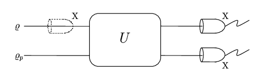
The above definition identifies the cloning of an observable with the cloning of its mean value. This is justified by the fact that for any single-qubit observable ${\rm X}$ the cloning of the mean value is equivalent to the cloning of the whole statistics. In fact, any ${\rm X}\in{\cal L}[{\mathbb{C}}^{2}]$ has at most two distinct eigenvalues $\{\lambda_{0},\lambda_{1}\}$, occurring with probability ${p_{0},p_{1}}$. For a degenerate eigenvalue the statement is trivial. For two distinct eigenvalues we have $\overline{\rm X}=\lambda_{1}p_{1}+\lambda_{0}p_{0}$ which, together with the normalization condition $1=p_{0}+p_{1}$, proves the statement. In other words, we say that the class of observables $\mathbf{X}$ has been cloned if a measurement of any ${\rm X}\in\mathbf{X}$ on either the two qubits at the output gives the same statistics as it was measured on the input signal qubit, independently on the initial qubit preparation.

A remark about this choice is in order. In fact, in view of the duality among states and operators on an Hilbert space, one may argue that a proper figure of merit to assess a cloning machine for observables would be a fidelity–like one. This is certainly true for the $d$-dimensional case, $d>2$, while for qubit systems a proper assessment can be also made in term of mean–value duplication, which subsumes all the information carried by the signal. Furthermore, in view of the possibility to realize a joint measurement via a cloner of observables, we recall that the Eq. Eq. (1) is a standard requirement in such a scenario, as already recalled in Sec. I

Before beginning our analysis let us illustrate a basic property of cloning machines, which follows from the definition, and which will be used throughout the paper. Given a cloning machine $\left(U,{\varrho_{p}},\mathbf{X}\right)$, then $\left(V,{\varrho_{p}},{\mathbf{Y}}\right)$ is a cloning machine too, where $V=(W^{\dagger}\otimes W^{\dagger})\>U\>(W\otimes\mathbb{I})$ and the class ${\mathbf{Y}}=W^{\dagger}\mathbf{X}W$ is formed by the observables $Y(j)=W^{\dagger}X(j)\,W$, $j\in{\cal J}$. The transformation $W$ may be a generic unitary. We will refer to this property to as unitary covariance of cloning machine. The proof proceeds as follows. By definition $\overline{\rm Y}(j)={\rm Tr}_{1}[\varrho\>W^{\dagger}X(j)W]={\rm Tr}_{1}[W\,\varrho\,W^{\dagger}\,{\rm X}(j)]$. Then, since $\left(U,{\varrho_{p}},\mathbf{X}\right)$ is a cloning machine, we have

	$\displaystyle\overline{\rm Y}(j)$	$\displaystyle={\rm Tr}_{1,2}[U\,(W\varrho\,W^{\dagger}\otimes{\varrho_{p}})\,U^{\dagger}\,({\rm X}(j)\otimes\mathbb{I})]$
		$\displaystyle={\rm Tr}_{1,2}[U\,(W\otimes\mathbb{I})(\varrho\otimes{\varrho_{p}})(W^{\dagger}\otimes\mathbb{I})\,U^{\dagger}\>(W\otimes W)({\rm Y}(j)\otimes\mathbb{I})(W^{\dagger}\otimes W^{\dagger})]$
		$\displaystyle={\rm Tr}_{1,2}[V\,(\varrho\otimes{\varrho_{p}})\,V^{\dagger}\,({\rm Y}(j)\otimes\mathbb{I})]=\overline{\rm Y}_{1}(j)\;.$		(3)

The same argument holds for $\overline{\rm Y}_{2}(j)$ note

Another result which will be used in the following is the parameterization of a two-qubit transformation, which corresponds to a ${\rm SU}(4)$ matrix, obtained by separating its local and entangling parts. A generic two-qubit gate ${\rm SU}(4)$ matrix may be factorized as follows car:

$\displaystyle U=L_{2}\,U_{\rm E}\,L_{1}=L_{2}\,\exp\Big[\frac{i}{2}\sum_{j=1}^{3}\theta_{j}\sigma_{j}\otimes\sigma_{j}\Big]\,L_{1}$

(4)

where $\theta_{j}\in\mathbb{R}$ and the $\sigma_{j}$’s are the Pauli’s matrices. The local transformations $L_{1}$ and $L_{2}$ belongs to the ${\rm SU}(2)\otimes{\rm SU}(2)$ group, whereas $U_{\rm E}$ accounts for the entangling part of the transformation $U$. In our context, decomposition (4), together with unitary covariance of cloning machines, allows to ignore the local transformations $L_{1}$, which corresponds to a different state preparation of signal and probe qubits at the input. On the other hand, as we will see in the following, the degree of freedom offered by the local transformations $L_{2}$ will be exploited to design suitable cloning machines for noncommuting observables.

In order to introduce cloning machines for a class of noncommuting observables let us consider the specific class $\mathbf{X}_{\rm nc}=\{x_{1}{\sigma_{1}}+x_{2}{\sigma_{2}}\}_{x_{1},x_{2}\in\mathbb{R}}$. If a cloning machine $(U,{\varrho_{p}},\mathbf{X}_{\rm nc})$ existed, then the mean values as well as the statistics of any observable belonging to $\mathbf{X}_{\rm nc}$ would be cloned at its output. As a consequence, one would jointly measure any two non-commuting observables belonging to $\mathbf{X}_{\rm nc}$ (e.g., ${\sigma_{1}}$ on the output signal and ${\sigma_{2}}$ on the output probe) without any added noise, thus violating the bounds imposed by quantum mechanics ake; ago; y82. Generalizing this argument to any two–parameter class of noncommuting observables (i.e., to any class $\mathbf{X}_{\rm gnc}=\{c\,{\rm C}+d\,{\rm D}\}_{c,d\in{\mathbb{R}}}$, with ${\rm C},\,{\rm D}$ generic non-commuting observables), we then conclude that a cloning machine for a generic two–parameter class of noncommuting observables does not exist jpa. This results resembles the no–cloning theorem for states, and it can actually be seen as its counterpart for cloning of observables. Furthermore, it permits a comparison among cloning machines for observables and for states. Let us write the generic input signal as $\varrho=\frac{1}{2}(\sigma_{0}+{\mathbf{s}}\cdot{\boldsymbol{\sigma}})$, where ${\boldsymbol{\sigma}}=(\sigma_{1},\sigma_{2},\sigma_{3})$, ${\boldsymbol{s}}=(s_{1},s_{2},s_{3})$ is the Bloch vector and $\sigma_{0}$ is the identity operator. The state–cloning counterpart of the statement above can then be obtained by considering the class of observables $\mathbf{X}_{\rm nc}$: If a cloning machine $(U,{\varrho_{p}},\mathbf{X}_{\rm nc})$ existed, then the components $s_{1}$ and $s_{2}$ of Bloch vector $\boldsymbol{s}$ would be cloned for any input signal. The same situation occurs in the case of a two–parameter class generated by any pair of Pauli operators. In other words, it is not possible to simultaneously copy a pair of components of the Bloch vector of a generic state, even completely disregarding the third one kie; app. Let us stress the fact that, even if a perfect cloning of observables could be performed (for example, in the case of a class generated by commuting observables jpa), correlations between the measurements would exist, otherwise state estimation limits would be overcame.

Now, a question arises on whether, analogously to state–cloning, we may introduce the concept of approximate cloning machines, i.e. cloning of observables involving added noise. Indeed this can be done and optimal approximate cloning machines corresponding to minimum added noise may be found as well.

An approximate cloning machine for the class of observables $\mathbf{X}$ is defined as the triple $(U,{\varrho_{p}},\mathbf{X})_{\rm apx}$ such that $\overline{\rm X}_{1}=\overline{\rm X}/g_{1}$ and $\overline{\rm X}_{2}=\overline{\rm X}/g_{2}$ i.e.

$\displaystyle\hbox{Tr}_{1}\left[\varrho\>{\rm X}\right]=g_{1}\hbox{Tr}_{12}\left[R\>{\rm X}\otimes\mathbb{I}\right]=g_{2}\hbox{Tr}_{12}\left[R\>\mathbb{I}\otimes{\rm X}\right]\>,$

(5)

for any ${\rm X}\in\mathbf{X}$. The quantities $g_{j}$, $j=1,2$ are independent on the input state and are referred to as the noises added by the cloning process.

Let us begin by again considering the class $\mathbf{X}_{\rm nc}=\{x_{1}{\sigma_{1}}+x_{2}{\sigma_{2}}\}_{x_{1},x_{2}\in\mathbb{R}}$. By using the decomposition of a generic ${\rm SU}(4)$ matrix in Eq. (4) one may attempt to find an approximate cloning machine considering only the action of the entangling kernel $U_{\rm E}$. Unfortunately, it can be shown that no $U_{\rm E}$, $g_{1}$ and $g_{2}$ exist which realize approximate cloning for ${\varrho_{p}}=|0\rangle\langle 0|$. A further single-qubit transformation should be introduced after $U_{\rm E}$. In particular, the unitary $F=i/\sqrt{2}(\sigma_{1}+\sigma_{2})$ flips the Pauli matrices ${\sigma_{1}}$ and ${\sigma_{2}}$ (i.e., $F^{\dagger}\sigma_{1,2}\,F=\sigma_{2,1}$) and permits the realization of an approximate cloning machine. Indeed, the unitary

$$T=(\mathbb{I}\otimes F)U_{\rm nc}\qquad U_{\rm nc}=e^{i\frac{\theta}{2}({\sigma_{1}}\otimes{\sigma_{1}}-{\sigma_{2}}\otimes{\sigma_{2}})}\>,$$

realizes the approximate cloning machine $(T,|0\rangle\langle 0|,\mathbf{X}_{\rm nc})_{\rm apx}$ with added noises

$\displaystyle g_{1}=\frac{1}{\cos\theta}\qquad g_{2}=\frac{1}{\sin\theta}\>.$

(6)

In order to prove the cloning properties of $T$ let us start from the unitary $(\mathbb{I}\otimes F)U_{\rm E}$, where $U_{\rm E}$ is a generic entangling unitary of the form given in Eq. (4). Then, by imposing approximate cloning for any ${\rm X}\in\mathbf{X}_{\rm nc}$, one obtains the following system of Equations:

	$\displaystyle g_{1}{\rm Tr}_{2}[(\mathbb{I}\otimes{\varrho_{p}})\,U_{E}^{\dagger}\,({\sigma_{1}}\otimes\mathbb{I})\,U_{E}]$	$\displaystyle={\sigma_{1}}$		(7a)
	$\displaystyle g_{1}{\rm Tr}_{2}[(\mathbb{I}\otimes{\varrho_{p}})\,U_{E}^{\dagger}\,({\sigma_{2}}\otimes\mathbb{I})\,U_{E}]$	$\displaystyle={\sigma_{2}}$		(7b)
	$\displaystyle g_{2}{\rm Tr}_{2}[(\mathbb{I}\otimes{\varrho_{p}})\,U_{E}^{\dagger}\,(\mathbb{I}\otimes{\sigma_{2}})\,U_{E}]$	$\displaystyle={\sigma_{1}}$		(7c)
	$\displaystyle g_{2}{\rm Tr}_{2}[(\mathbb{I}\otimes{\varrho_{p}})\,U_{E}^{\dagger}\,(\mathbb{I}\otimes{\sigma_{1}})\,U_{E}]$	$\displaystyle={\sigma_{2}}\>.$		(7d)

System (7) admits the solution $\theta_{1}=-\theta_{2}=\theta/2$, $\theta_{3}=0$—i.e., $U_{E}\equiv U_{\rm nc}$ with $\theta$ free parameter—with $g_{1}=1/\cos\theta$ and $g_{2}=1/\sin\theta$. Notice that other solutions for the $\theta_{1,2,3}$’s parameters may be found, which however give the same added noise as the one considered above.

Remarkably, similar cloning machines may be obtained for any class of observables generated by a pair of operators unitarily equivalent to ${\sigma_{1}}$ and ${\sigma_{2}}$. In fact, given the two-parameter classes of noncommuting observables defined as $\mathbf{X}_{\rm V}=\{c\,{\rm C}+d\,{\rm D}\}_{c,d\in{\mathbb{R}}}$, with ${\rm C}=V^{\dagger}{\sigma_{1}}V$, ${\rm D}=V^{\dagger}{\sigma_{2}}V$ and $V$ generic unitary one has that an approximate cloning machine is given by the triple $(U_{V},|0\rangle\langle 0|,\mathbf{X}_{\rm V})_{\rm apx}$, with $U_{V}=(V^{\dagger}\otimes V^{\dagger})(\mathbb{I}\otimes F)\>U_{\rm nc}\>(V\otimes\mathbb{I})$, with added noises $g_{1}=1/\cos\theta$ and $g_{2}=1/\sin\theta$. The statement easily follows from the fact that $(T,|0\rangle\langle 0|,\mathbf{X}_{\rm nc})_{\rm apx}$ is a cloning machine and from unitary covariance. Similar results hold for any class of observables unitarily generated by any pair of (noncommuting) Pauli operators.

Let us now consider if the approximate cloning machine for observables introduced above is optimal. In order to assess the quality and to define optimality of a triple $(U,{\varrho_{p}},\mathbf{X})_{\rm apx}$ we consider it as a tool to perform a joint measurements of noncommuting qubit observables tri. For example, consider the cloning machine $(T,|0\rangle\langle 0|,\mathbf{X}_{\rm nc})_{\rm apx}$ and suppose to measure ${\sigma_{1}}$ and ${\sigma_{2}}$ on the two qubits at the output. We emphasize again that the cloning machine $(T,|0\rangle\langle 0|,\mathbf{X}_{\rm nc})_{\rm apx}$ clones every observable belonging to $\mathbf{X}_{\rm nc}$, while we are now considering only the observables ${\sigma_{1}}$ and ${\sigma_{2}}$ which, in a sense, generate the class. The difference with a joint measurement specifically designed to measure only a couple of observables is evident. Indeed a priori it is not clear at all if a cloning for observables, being in this sense far more general than a joint measurement, can reach the minimum disturbance necessary to perform an optimal joint measurement. Nevertheless, this turns out to be the case, as we will see in the following. We have that the measured expectation values of ${\sigma_{1}}$ and ${\sigma_{2}}$ at the output are given by $\langle\sigma_{h}\rangle_{\rm m}=g_{h}\langle\sigma_{h}\rangle$ (with $h=1,2$), where the $\langle\sigma_{h}\rangle$’s are the input mean values. It follows that the measured uncertainties ($\Delta O=\langle O^{2}\rangle-\langle O\rangle^{2}$) at the output are given by

$$\Delta_{\rm m}\sigma_{h}=g_{h}^{2}\Delta_{\rm i}\sigma_{h}$$

where $\Delta_{\rm i}\sigma_{h}$ denote the intrinsic uncertainties for the two quantities at the input. Since for any Pauli operators we have $\sigma_{h}^{2}=\mathbb{I}$ one may rewrites

	$\displaystyle\Delta_{\rm m}{\sigma_{1}}$	$\displaystyle=\tan^{2}\theta+\Delta_{\rm i}{\sigma_{1}}$		(8)
	$\displaystyle\Delta_{\rm m}{\sigma_{2}}$	$\displaystyle=\cot^{2}\theta+\Delta_{\rm i}{\sigma_{2}}\>.$		(9)

As a consequence, the measured uncertainty product is given by:

$$\Delta_{\rm m}{\sigma_{1}}\Delta_{\rm m}{\sigma_{2}}=\Delta_{\rm i}{\sigma_{1}}\Delta_{\rm i}{\sigma_{2}}+\cot^{2}\theta\Delta_{\rm i}{\sigma_{1}}+\tan^{2}\theta\Delta_{\rm i}{\sigma_{2}}+1\>.$$

Since the arithmetic mean is bounded from below by the geometric mean we have

$$\cot^{2}\theta\Delta_{\rm i}{\sigma_{1}}+\tan^{2}\theta\Delta_{\rm i}{\sigma_{2}}\geq 2\sqrt{\Delta_{\rm i}{\sigma_{1}}\Delta_{\rm i}{\sigma_{2}}}\>,$$

with the equal sign iff $\Delta_{\rm i}{\sigma_{1}}=\tan^{4}\theta\Delta_{\rm i}{\sigma_{2}}$, then it follows that

$$\Delta_{\rm m}{\sigma_{1}}\Delta_{\rm m}{\sigma_{2}}\geq\left(\sqrt{\Delta_{\rm i}{\sigma_{1}}\Delta_{\rm i}{\sigma_{2}}}+1\right)^{2}\>.$$

If the initial signal is a minimum uncertainty state—i.e., $\Delta_{\rm i}{\sigma_{1}}\Delta_{\rm i}{\sigma_{2}}=1$—one finally has that the measured uncertainty product is bounded by $\Delta_{\rm m}{\sigma_{1}}\Delta_{\rm m}{\sigma_{2}}\geq 4$. Notice that an optimal joint measurement corresponds to have $\Delta_{\rm m}{\sigma_{1}}\Delta_{\rm m}{\sigma_{2}}=4$. In our case this is realized when $\theta$ is chosen such that $\tan^{4}\theta=\Delta_{\rm i}{\sigma_{1}}/\Delta_{\rm i}{\sigma_{2}}$. As already recalled in Sec. I, such an a priori knowledge of the initial state is a standard requirement of joint measurements. Therefore, since $(T,|0\rangle\langle 0|,\mathbf{X}_{\rm nc})_{\rm apx}$ adds the minimum amount of noise in a joint measurement performed on minimum uncertainty states we conclude that it is an optimal approximate cloning machine for the class under investigation. An optimal approximate cloning machine for the more general class $\mathbf{X}_{\rm gnc}$ may be also defined, using the concept of joint measurement for noncanonical observables tri.

Let us now consider the comparison with a joint measurement of ${\sigma_{1}}$ and ${\sigma_{2}}$ performed with the aid of an optimal universal cloning machine for states buz. It is easy to show that the best result in this case is given by $\Delta_{\rm m}{\sigma_{1}}\Delta_{\rm m}{\sigma_{2}}=\frac{9}{2}$, indicating that cloning of observables is more effective than cloning of states to perform joint measurements (for the case of three observables see Refs. hil; pva). In fact, a symmetric cloning machine for states shrinks the whole Bloch vector $\boldsymbol{s}$ by a factor $\frac{2}{3}$, whereas a cloning machine for observables shrinks the components $s_{1}$ and $s_{2}$ of $\boldsymbol{s}$ only by a factor $1/\sqrt{2}$ (considering equal noise $g_{1}=g_{2}=\sqrt{2}$). Notice that such a behavior is different from what happens in the case of continuous variables, for which the optimal covariant cloning of coherent states also provides the optimal joint measurements of two conjugated quadratures cer. This is due to the fact that coherent states are fully characterized by their complex amplitude, that is by the expectation values of two operators only, whereas the state of a qubit requires the knowledge of the three components of the Bloch vector.

As a final remark we notice that if the requirement of universality is dropped, then cloning machines for states can be found that realize optimal approximate cloning of observables. For example, an approximate cloning machine for the two–parameter class $\mathbf{X}_{\rm nc}$ can be obtained by considering a phase–covariant cloning for states phc. In order to clarify this point, let us recall that a phase–covariant cloning machine for states of the form uses a probe in the $|0\rangle$ state and performs the following transformation:

	$\displaystyle|0\rangle|0\rangle$	$\displaystyle\rightarrow|0\rangle|0\rangle$
	$\displaystyle|1\rangle|0\rangle$	$\displaystyle\rightarrow\cos\theta|1\rangle|0\rangle+\sin\theta|0\rangle|1\rangle)\,,$		(10)

where, in general, $\theta\in[0,2\pi]$. If we now consider the $\mathbf{X}_{\rm nc}$ class it is straightforward to show that Eqs. (5) are satisfied for any ${\rm X}\in\mathbf{X}_{\rm nc}$ using the machine (10), with the optimal added noises given by Eq. (6). This can be intuitively understood by considering that a phase covariant cloning machine extracts the optimal information about states lying on the equatorial plane of the Bloch sphere, which in turn include the eigenstates of $\sigma_{1}$ and $\sigma_{2}$. Nevertheless, notice that there exist optimal approximate cloning machines for observables which do not coincide with phase–covariant cloning for states. As an example, considering a cloning machine with added noise $g_{1}=-1/\cos\theta$ and $g_{2}=-1/\sin\theta$ one would still obtain optimal cloning of observables, even if such a machine could not perform a phase covariant cloning of states. This remark shows that, in general, one cannot simply transfer the results for state cloning into the cloning of observables case.

We have analyzed in details the cloning for classes of observables with focus on classes generated by two noncommuting observables. We have elucidated the relationship between cloning of observables and joint measurements and shown that even if the cloning machine is designed to act on the whole class generated by two noncommuting observables, the same optimal performances of a joint measurement can be attained.

This work has been supported by MIUR through the project PRIN-2005024254-002. AF acknowledges the financial support from Università di Milano under Grant “Borse di perfezionamento all’estero”.

References

- (1) E. Arthurs, J. L. Kelly, Bell. Sys. Tech. J. 44, 725 (1965).
- (2) N. J. Cerf et al, Phys. Rev. Lett. 85, 1754 (2000).
- (3) N. Gisin and S. Massar, Phys. Rev. Lett. 79, 2153 (1997); D. Bruss, A. Ekert, and C. Macchiavello, Phys. Rev. Lett. 81, 2598 (1998); J. Bae and A. Acin, e–print quant-ph/0603078.
- (4) E. Arthurs, M. S. Goodman, Phys. Rev. Lett. 60, 2447 (1988).
- (5) H. P. Yuen, Phys. Lett. A91, 101 (1982).
- (6) A. Trifonov et al., Phys. Rev. Lett. 86, 4423 (2001).
- (7) V. Buzek and M. Hillery, Phys. Rev. A 54, 1844 (1996).
- (8) C. -S. Niu and R. B. Griffiths, Phys. Rev. A 60, 2764 (1999). D. Bruss et al, Phys. Rev. A 62, 012302 (2000).
- (9) A. Ferraro, M. Galbiati, and M.G.A. Paris, J. Phys. A: Math. Gen. 39, L219 (2006).
- (10) see e.g. R. R. Tucci, e–print quant-ph/0507171.
- (11) Notice that a cloning machine of the form with , where is an arbitrary unitary matrix also assures that . On the other hand, in order to have at the same time, the relation should hold.
- (12) P. Kienzler, Int. J. Th. Phys. 37, 257 (1998).
- (13) D. M. Appleby, Int. J. Th. Phys. 39, 2231 (2000).
- (14) V. Buzek et al, Phys. Rev. A 56, 3446 (1997).
- (15) G. M. D’Ariano et al, J. Opt. B 3, 44 (2001).