Decoherence-induced geometric phase in a multilevel atomic system
Abstract
We consider the STIRAP process in a three-level atom. Viewed as a closed system, no geometric phase is acquired. But in the presence of spontaneous emission and/or collisional relaxation we show numerically that a non-vanishing, purely real, geometric phase is acquired during STIRAP, whose magnitude grows with the decay rates. Rather than viewing this decoherence-induced geometric phase as a nuisance, it can be considered an example of “beneficial decoherence”: the environment provides a mechanism for the generation of geometric phases which would otherwise require an extra experimental control knob.
I Introduction
Berry observed that quantum systems may retain a memory of their motion in Hilbert space through the acquisition of geometric phases Berry:84. Remarkably, these phase factors depend only on the geometry of the path traversed by the system during its evolution. Soon after this discovery, geometric phases became a subject of intense theoretical and experimental studies Wilczek:book. In recent years, renewed interest has arisen in the study of geometric phases in connection with quantum information processing Zanardi:99b; Jones:00. Indeed, geometric, or holonomic quantum computation (QC) may be useful in achieving fault tolerance, since the geometric character of the phase provides protection against certain classes of errors Solinas:04; Zhu:05; Fuentes-Guridi:05; WuZanardiLidar:05. However, a comprehensive investigation in this direction requires a generalization of the concept of geometric phases to the domain of open quantum systems, i.e., quantum systems which may decohere due to their interaction with an external environment.
Here we consider the following basic question:
Is it possible for the environment to induce a geometric phase where there is none if the system is treated as closed?
Apart from its fundamental nature, this question is of obvious practical importance to holonomic QC, since if the anwer is affirmative the corresponding open-system geometric phase can either be detrimental (if it causes a deviation from the intended value) or beneficial, in the sense that the environment is acting as an amplifier for, or even generator of, the geometric phase.
Geometric phases in open systems, and more recently their applications in holonomic QC, have been considered in a number of works, since the late 1980’s. The first, phenomenological approach to the subject used the Schrödinger equation with non-Hermitian Hamiltonians Garrison:88; Dattoli:90. While a consistent non-Hermitian Hamiltonian description of an open system in general requires the theory of stochastic Schrödinger equations Gardiner:book, this phenomenological approach for the first time indicated that complex Abelian geometric phases should appear for systems undergoing cyclic evolution. In Refs. Ellinas:89; Gamliel:89; Romero:02; Whitney:03; Whitney:05; Kamleitner:04, geometric phases acquired by the density operator were analyzed for various explicit models within a master equation approach. In Refs. Carollo:03; Fuentes-Guridi:05, the quantum jumps method was employed to provide a definition of geometric phases in Markovian open systems (related difficulties with stochastic unravellings have been pointed out in Ref. Bassi:05). In another approach the density operator, expressed in its eigenbasis, was lifted to a purified state Tong:04; Rezakhani:05. In Ref. Marzlin:04, a formalism in terms of mean values of distributions was presented. An interferometric approach for evaluating geometric phases for mixed states evolving unitarily was introduced in Ref. Vedral:00 and extended to non-unitary evolution in Refs. Faria:03; Ericsson:03. This interferometric approach can also be considered from a purification point of view Vedral:00; Ericsson:03. This multitude of different proposals revealed various interesting facets of the problem. Nevertheless, the concept of adiabatic geometric phases in open systems remained unresolved in general, since most of these treatments did not employ an adiabatic approximation genuinely developed for open systems. Note that the applicability of the closed systems adiabatic approximation Messiah:vol2 to open systems problems is not a priori clear and should be justified on a case-by-case basis. Moreover, almost all of the previous works on open systems geometric phases were concerned with the Abelian (Berry phase) case. Exceptions are the very recent Refs. Fuentes-Guridi:05; Florio:06; Trullo:06, which discuss both non-adiabatic and adiabatic dynamics, but employ the standard adiabatic theorem for closed systems in the latter case.
Recently, a fully self-consistent approach for both Abelian and non-Abelian adiabatic geometric phases in open systems was proposed by Sarandy and Lidar (SL) in Ref. SarandyLidar:06. It applies to the very general class of systems described by convolutionless master equations Breuer:book. SL made use of the formalism they developed in Ref. SarandyLidar:04 for adiabaticity in open systems, which relies on the Jordan normal form of the relevant Liouville (or Lindblad) super-operator. The geometric phase was then defined in terms of the left and right eigenvectors of this super-operator. This definition is a natural generalization of the one given by Berry for a closed system, and was shown to have a proper closed system limit. The formalism was illustrated in Ref. SarandyLidar:06 in the context of a spin system interacting with an adiabatically varying magnetic field.
In order to address the basic question posed above, we study here the adiabatic geometric phase in a multi-level atomic system using the SL formalism. Specifically, we consider the process of stimulated Raman adiabatic passage (STIRAP) Bergmann:98; Unanyan:99 in a three-level atomic system in a configuration. We analyze a version of STIRAP where the closed system geometric phase is identically zero. We then show that when spontaneous emission and/or collisional relaxation are included, the same STIRAP process yields a non-vanishing geometric phase. This decoherence-induced geometric phase is an example of “beneficial decoherence”, where the environment performs a potentially useful task. This is conceptually similar to the phenomenon of decoherence-induced entanglement Plenio:99; PhysRevA.65.040101.
Since the SL formalism involves finding the Jordan normal form of a general matrix, which is an analytically difficult problem, we developed a numerically stable program to find the Jordan form of any complex square matrix and used it to find the geometric phase program.
The structure of the paper is as follows. In Section II we briefly review the STIRAP process in a closed three level system in the configuration, and the corresponding calculation of the (vanishing) geometric phase. In Section III we revisit this problem in the open system setting and derive the solution of the STIRAP model. Our numerical results, along with a detailed analysis of the geometric phase, are presented in Section IV. We conclude in Section V.
II Geometric Phase under STIRAP: The Closed System Case
We consider the process of stimulated Raman adiabatic passage (STIRAP) Bergmann:98 in a three-level system in the configuration, as shown in Fig. 1.

In this process, the initial atomic population in level is completely transferred to level , while the pulses are applied in a “counterintuitive” sequence. The intermediate level does not become substantially populated. The interaction picture Hamiltonian in one-photon resonance can be written in the rotating-wave approximation as follows:
| (1) |
where the real functions are the time-dependent Rabi frequencies of the two laser pulses, interacting respectively with the transitions (). The eigenvalues of are given by
| (2) |
and the respective eigenvectors are given by
where . Thus the time-dependence of the eigenfunctions is parameterized by that of . In principle the ’s can be complex valued, which gives rise to a controllable phase WuZanardiLidar:05. Here we work with real valued ’s and set for the remainder of this work. The state is a dark state, i.e., it has eigenvalue .
We choose a Gaussian time-dependent profile for the control pulses:
| (4) |
where and are the pulse amplitudes, and is the time-delay between the pulses, with pulse preceding pulse . All time-scales are normalized in terms of the pulse-width . The closed-system adiabaticity condition is satisfied provided and Bergmann:98
| (5) |
In this limit, the evolution of the system strictly follows the evolution of either of the adiabatic states. Due to the ordering of the pulses as in (4), the atom initially in the level is prepared in the adiabatic state . The population in level is then completely transferred to level adiabatically, following the evolution of state under the action of the pulses (4). Note that as the system follows the evolution of the state in the adiabatic limit and the excited level does not contribute to , the traditional view of the process is that it remains unaffected by spontaneous emission. Below we will show how this view must be modified in a consistent treatment of the process as evolution of an open system. In addition, incoherent processes such as dephasing of the ground state levels will affect the population transfer process.
The geometric phases acquired by each adiabatic state , as acquired during the evolution between and can be easily calculated from Berry:84
| (6) |
In terms of a vector in parameter space undergoing cyclic evolution, this phase can be rewritten as
| (7) |
In the case of the three-level system depicted in Fig. 1, the parameter space is defined by and , i.e.,
| (8) |
We consider a cyclic evolution in this parameter space, which takes place as varies from to , i.e., , . This is shown in Fig. 2.

One can also parametrize the time-dependence of the pulses in terms of an angle , using (4), such that
| (9) |
Then as varies from to we have that varies from to , and hence varies from to . Changing variables in Eq. (7), the geometric phase becomes in our case:
| (10) |
Note that the relevant parameter space for our problem is that with coordinates , not of Eq. (); indeed, Eq. (10) does not even describe a cycle in the space, whereas the expression (8) along with Fig. 2 show clearly that there is a cycle in the space.
Let us now show that the geometric phase vanishes for all three adiabatic eigenstates of (), because the integrand . Indeed, consider the adiabatic eigenstates of Eq. (). Then , and , irrespective of the value of . Also, . Thus the STIRAP process under consideration does not give rise to a closed-system geometric phase. We note that the analysis above is a special case of the four-level model considered in Ref. Unanyan:99.
III Geometric Phase under STIRAP: The Open System Case
III.1 The model
We now analyze the effect on the geometric phase of interaction of the atomic system with a bath causing spontaneous emission and collisional relaxation. We describe these processes in the Markovian limit for the bath, using time-independent Lindblad operators and neglecting Lamb and Stark shift contributions Breuer:book. Thus the time-dependence appears only in the control Hamiltonian [Eq. (1)], and the evolution of the system density matrix is given by the Lindblad equation (in units):
| (11) |
where the dissipator describes the incoherent processes, arising from system-bath interaction. We include spontaneous emission from level at rates and via Lindblad operators
| (12) |
We also include collisional relaxation between levels and at rates and via Lindblad operators
| (13) |
III.2 Review of open systems geometric phase
To see how a geometric phase can be associated with the master equation evolution, we follow Ref. SarandyLidar:06 and write the master equation as
| (14) |
where depends on time only through a set of parameters . These parameters will undergo adiabatic cyclic evolution in our problem.
In the superoperator formalism, the density matrix for a quantum state in a -dimensional Hilbert space is represented by a -dimensional “coherence vector” (where denotes the transpose) and the Lindblad superoperator becomes a -dimensional supermatrix Alicki:87, so that the master equation (14) can be written as linear vector equation in -dimensional Hilbert-Schmidt space, in the form . Such a representation can be generated, e.g., by introducing a basis of Hermitian, trace-orthogonal, and traceless operators [e.g., the -dimensional irreducible representation of the generators of su()], whence the are the expansion coefficients of in this basis Alicki:87, with the coefficient of (the identity matrix).
The master equation generates a non-unitary evolution since is non-Hermitian. In fact, need not even be a normal operator (). Therefore is generally not diagonalizable, i.e., it does not possess a complete set of linearly independent eigenvectors. Equivalently, it cannot be put into diagonal form via a similarity transformation. However, one can always apply a similarity transformation to which puts it into the (block-diagonal) Jordan canonical form Horn:book, namely, . The Jordan form of a matrix is a direct sum of blocks of the form ( enumerates Jordan blocks), where is the number of linearly independent eigenvectors of , where is the dimension of the th Jordan block, and where is the th (generally complex-valued) Lindblad-Jordan (LJ) eigenvalue of (obtained as roots of the characteristic polynomial), is the dimensional identity matrix, and is a nilpotent matrix with elements (’s above the main diagonal), where is the Kronecker symbol. Since the sets of left and right eigenvectors of are incomplete (they do not span the vector space), they must be completed to form a basis. Instantaneous right and left bi-orthonormal bases in Hilbert-Schmidt space can always be systematically constructed by adding new orthonormal vectors to the th left or right eigenvector, such that they obey the orthonormality condition SarandyLidar:04. Here superscripts enumerate basis states inside a given Jordan block (). When is diagonalizable, and are simply the bases of right and left eigenvectors of , respectively. If is not diagonalizable, these right and left bases can be constructed by suitably completing the set of right and left eigenvectors of (which can be identified with columns of and , respectively, associated with distinct eigenvalues ). Then for all times
so that the and preserve the Jordan block structure (see Appendix A of Ref. SarandyLidar:06 for a detailed discussion of these issues).
In order to define geometric phases in open systems, the coherence vector is expanded in the instantaneous right vector basis as
| (15) |
where the dynamical phase is explicitly factored out. The coefficients play the role of “geometric” (non-dynamical) amplitudes. We assume that the open system is in the adiabatic regime, i.e., Jordan blocks associated to distinct eigenvalues evolve in a decoupled manner SarandyLidar:04. Then:
| (16) |
Note that, due to the restriction , the dynamical phase has disappeared.
A condition on the total evolution time, which allows for the neglect of coupling between Jordan blocks used in deriving Eq. (16), was given in Ref. SarandyLidar:04. This condition generalizes the standard closed-system adiabaticity condition Messiah:vol2, from which Eq. (5) is derived. Nevertheless, we have used the simpler condition (5) in our simulations below, as it is rather accurate in the present open system case.
For closed systems, Abelian geometric phases are associated with non-degenerate levels of the Hamiltonian, while non-Abelian phases appear in the case of degeneracy. In the latter case, a subspace of the Hilbert space acquires a geometric phase which is given by a matrix rather than a scalar. For open systems, one-dimensional Jordan blocks are associated with Abelian geometric phases in the absence of degeneracy, or with non-Abelian geometric phases in case of degeneracy. Multi-dimensional Jordan blocks are always tied to a non-Abelian phase SarandyLidar:06.
III.2.1 The Abelian case: generalized Berry phase
Consider the simple case of a non-degenerate one-dimensional Jordan block (a block that that is a submatrix containing an eigenvalue of ). In this case, the absence of degeneracy implies in Eq. (16) that (non-degenerate blocks). Moreover, since the blocks are assumed to be one-dimensional we have , which allows for removal of the upper indices in Eq. (16), resulting in . The solution of this equation is , with . For a cyclic evolution in parameter space along a closed curve , one then obtains the Abelian geometric phase associated with the Jordan block SarandyLidar:06:
| (17) |
This expression for the geometric phase bears clear similarity to the original Berry formula, Eq. (7). Note that in general can be complex, since and are not related by transpose conjugation. Thus, the geometric phase may have real and imaginary contributions, the latter affecting the visibility of the phase. As shown in Ref. SarandyLidar:06, the expression above for satisfies a number of desirable properties: it is geometric (i.e., depends only on the path traversed in parameter space), it is gauge invariant (i.e., one cannot modify the geometric phase by redefining or via multiplication of one of them by a complex factor); it has the proper closed system limit (if the interaction with the bath vanishes, reduces to the usual difference of geometric phases acquired by the density operator in the closed case).
III.2.2 The non-Abelian case
Ref. SarandyLidar:06 also derived the non-Abelian open systems geometric phase, for the case of degenerate one-dimensional Jordan blocks. A non-Abelian geometric phase in fact arises in our STIRAP model when the spontaneous emission rates are equal. However, we shall not treat this case in the present paper.
III.3 Solution of the STIRAP model
Returning to the STIRAP model, let us represent the density matrix in terms of the coherence vector as
| (18) |
where the are the Gell-Mann matrices Gellmann:book. Writing the Lindblad equation in the basis, we obtain , where is a nine-component coherence vector. In the same basis we can express the Liouville operator in the following form:
| (19) |
where we have used the Hamiltonian (1). Here
| (20) |
and are given in Eq. (4).
The eigenvalues and left and right eigenvectors of can be found in terms of the parameters and , but the expressions are very complicated. The analytic determination of the corresponding left and right eigenvectors is cumbersome, so instead we have used a numerical procedure, which is based on the discussion presented in subsection III.2 above program.
To exhibit some of the analytic structure, we temporarily make the further simplification that the spontaneous emission rates are equal: . This is the case, e.g., for transitions in 23Na sodium. In addition we assume temporarily that the collisional relaxation rates vanish:. With these simplifications has the following three sets of eigenvalues (the ordering of subscripts is explained below):
where
| (22) |
and the last set of four eigenvalues appears in two degenerate pairs. Because of this, the corresponding open systems geometric phase is non-Abelian (recall the discussion above), but we do not consider this case here.
In the closed system limit () becomes and its eigenvalues are (), where are the eigenvalues of the control Hamiltonian as given in Eq. (2). The grouping in Eq. (III.3) represents this limit in the following sense:
| (23) |
The corresponding eigenvectors of reduce to . The subscripts of the represents the ordering of the eigenvalues in the closed system limit. We find that the degeneracy leading to a non-Abelian geometric open system phase appears only when and , or in the closed system limit.
By a coordinate transformation from the control fields to the angle we have, similarly to the closed system case, from the generalized geometric phase formula Eq. (17):
| (24) |
This expression for the phase associated with the th eigenvector of yields, in the closed system limit, not the absolute phase of each of the adiabatic eigenstates of the system Hamiltonian, but rather their phase differences. This is natural as only a phase difference is an experimentally measurable quantity.
IV Results and Discussion


We plot the real part of the open system Abelian geometric phase, i.e., Eq. (24), for various combinations of the spontaneous emission and collisional relaxation rates in Figs. 3-10. The main finding is that the answer to the question we posed in the introduction, “Is it possible for the environment to induce a geometric phase where there is none if the system is treated as closed?”, is affirmative. Indeed, a glance at Figs. 3-10 reveals that the geometric phase is non-zero, and in fact increases with the decay rates. Moreover, we find that the imaginary part of the geometric phase is always zero to within our numerical accuracy, implying that the visibility of the geometric phase is unaffected in the present case by the interaction with the environment.


In Fig. 3 we show the real part of the open system geometric phases and , for the case when collisional relaxation vanishes () and there is only spontaneous emission (). Clearly, the phases increase monotonically with the emission rates. It is interesting to note that (to within our numerical accuracy) when . Recalling that and [Eq. (23)], this symmetry can be traced back to the difference between the adiabatic eigenstates and , which differ only in the sign of the coefficient in front of the excited state [recall Eq. () and that ]. When the spontaneous emission rates are equal this difference in sign between the ( component of the) states and generates only a difference in sign between the corresponding geometric phases, but not in magnitude, i.e., .


We also note that, in spite of the symmetry between the states and in our model, there is an asymmetry between the curves and in Fig. 3 for a given geometric phase, e.g., . Indeed, one might have expected a symmetry under interchange of the indices and , in the sense that, e.g., the points and on the curves and respectively, should have overlapped. That this is not the case is because the order of the pulses (first) and (second) breaks the symmetry between states and . Indeed, Fig. 4 shows the results for when the pulse order is reversed (now precedes ), and as a consequence the order of the curves and is now reversed as well. In other words, swapping the pulse order is equivalent to swapping the spontaneous emission rates and .
In Fig. 5 we show the real part of the open system geometric phases and , for the case when spontaneous emission vanishes () and there is only collisional relaxation (). The results are qualitatively similar to those in Fig. 3, with the exception that now when . This symmetry breaking can be attributed to the fact that the collisional relaxation operators directly connect the states and , whereas these states are only connected to second order under spontaneous emission and under the control Hamiltonian (1). The other interesting difference between Figs. 3 and 5 is that spontaneous emission only leads to larger values of the geometric phase than collisional relaxation only.
In Figs. 6-9 we show the real part of the open system geometric phases and . All four phases involve the dark state in the closed system limit. Recall from Eq. (23) that the pair of eigenvalues becomes degenerate in the closed system limit, as does the pair . Figures 6 and 7 show the case of vanishing collisional relaxation but non-vanishing spontaneous emission. Figures 8 and 9 shows the opposite case of non-vanishing collisional relaxation but vanishing spontaneous emission. It is interesting to observe that when there is only spontaneous emission, as in Figs. 6 and 7, the phases corresponding to degenerate eigenvalues in the closed system limit are identical to within our numerical precision. We do not have an intuitive explanation for this symmetry, which is absent when there is only collisional relaxation, as in Figs. 8 and 9. On the other hand, the asymmetry between Figs. 6 and 7 and between Figs. 8 and 9, can again be attributed to the symmetry breaking between levels and , due to the time ordering of the control pulses.
In Fig. 10 we revisit and , and turn on both spontaneous emission and collisional relaxation, and consider irrational ratios of the various decay rates (in order to eliminate potential accidental degeneracies due to rational ratios). Indeed, all six curves are clearly separated, and judging by comparison to Fig. 3, the effect of including both decoherence mechanisms is to increase the magnitude of the geometric phases (i.e., the decoherence mechanisms cooperate rather than interfere).

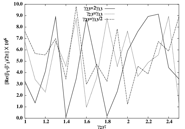
As a final note, we should point out that varying the Rabi frequencies and along a closed cycle in parameter space (Fig. 2), i.e., letting the time vary from to (which we implement in practice by integrating from to ), is incompatible with Eq. (5) for all times due to the finiteness of the parameters involved. Indeed, Fig. 11 shows the left-hand side of Eq. (5) for the parameters we have used in our simulations. It is clear that the adiabaticity condition is satisfied only for , where and . However, when we repeat our calculations of the open system geometric phase with varying between angles and corresponding to the times and (i.e., not along a complete cycle in the parameter space), we find – as can be seen in Fig. 12 – that the effect on the geometric phase is entirely negligible. This confirms that our choice of parameters satisfies the adiabatic limit for all practical purposes.

V Conclusions
Our study of STIRAP in an open three level quantum system reveals that the interaction with the environment can endow a system with a geometric phase, where none existed without the interaction with the environment. Mathematically, the vanishing geometric phase in the closed system case is attributable to the vanishing integrand in the Berry formula. In a certain sense this is easily understood as the result of having a geometric phase determined by only a single parameter (), whence no solid angle is traced out in parameter space. It would then be natural to conclude that, by including the interaction with the environment a non-zero solid angle is created, implying that in the presence of decoherence motion along an orthogonal direction in parameter space must have taken place. However, one must be careful in accepting this explanation, since in fact the polar angles and do not properly describe the parameter space in our problem: indeed, varies from to (while is constant) and thus does not describe a closed path, while the correct parameter space is that defined by the pulse amplitudes and (see Fig. 2). Thus a proper explanation of the intriguing effect of an environmentally induced geometric phase is still lacking and will be undertaken in a future publication. Here we conjecture that this is due to the non-commutativity of the driving Hamiltonian and the decohering processes we have considered. It should be possible to test this by using the quantum trajectories approach to the open systems geometric phase Fuentes-Guridi:05. Another interesting open question is to what extent the finding presented here can be made useful in the context of holonomic quantum computing Zanardi:99b, i.e., whether can one constructively exploit the environmentally induced geometric phase for the generation of quantum logic gates.
References
- (1) M.V. Berry, Proc. Roy. Soc. London Ser. A 392, 45 (1984).
- (2) Geometric Phases in Physics, edited by A. Shapere and F. Wilczek (World Scientific, Singapore, 1989).
- (3) P. Zanardi, Phys. Lett. A 264, 94 (1999).
- (4) J. A. Jones, V. Vedral, A. Ekert, and G. Castagnoli, Nature 403, 869 (2000).
- (5) P. Solinas, P. Zanardi, and N. Zangh, Phys. Rev. A 70, 042316 (2004).
- (6) L.-A. Wu, P. Zanardi, and D.A. Lidar, Phys. Rev. Lett. 95, 130501 (2005).
- (7) S.-L. Zhu and P. Zanardi, Phys. Rev. A 72, 020301(R) (2005).
- (8) I. Fuentes-Guridi, F. Girelli, and E. Livine, Phys. Rev. Lett. 94, 020503 (2005).
- (9) J. C. Garrison and E. M. Wright, Phys. Lett. A 128, 177 (1988).
- (10) G. Dattoli, R. Mignani, and A. Torre, J. Phys. A 23, 5795 (1990).
- (11) C.W. Gardiner and P. Zoller, Quantum Noise, Vol. 56 of Springer Series in Synergetics (Springer, Berlin, 2000).
- (12) D. Ellinas, S. M. Barnett, and M. A. Dupertuis, Phys. Rev. A 39, 3228 (1989).
- (13) D. Gamliel and J. H. Freed, Phys. Rev. A 39, 3238 (1989).
- (14) K. M. F. Romero, A. C. A. Pinto, and M. T. Thomaz, Physica A 307, 142 (2002).
- (15) R. S. Whitney and Y. Gefen, Phys. Rev. Lett. 90, 190402 (2003).
- (16) R. S. Whitney, Y. Makhlin, A. Shnirman, and Y. Gefen, Phys. Rev. Lett. 94, 070407 (2005).
- (17) I. Kamleitner, J. D. Cresser, and B. C. Sanders, Phys. Rev. A 70, 044103 (2004).
- (18) A. Carollo, I. Fuentes-Guridi, M. Franca Santos, and V. Vedral, Phys. Rev. Lett. 90, 160402 (2003).
- (19) A. Bassi and E. Ippoliti, Phys. Rev. A 73, 062104 (2006).
- (20) D. M. Tong, L. C. Kwek, C. H. Oh, J.-L. Chen, and L. Ma, Phys. Rev. A 69, 054102 (2004).
- (21) A. T. Rezakhani and P. Zanardi, Phys. Rev. A 73, 012107 (2006).
- (22) K.-P. Marzlin, S. Ghose, and B. C. Sanders, Phys. Rev. Lett. 93, 260402 (2004).
- (23) E. Sjöqvist, A. K. Pati, A. Ekert, J. S. Anandan, M. Ericsson, D. K. L. Oi, and V. Vedral, Phys. Rev. Lett. 85, 2845 (2000).
- (24) J. G. P. de Faria, A. F. R. de Toledo Piza, and M. C. Nemes, Europhys. Lett. 62, 782 (2003).
- (25) M. Ericsson, E. Sjöqvist, J. Brännlund, D. K. L. Oi, A. K. Pati, Phys. Rev. A 67, 020101(R) (2003).
- (26) A. Messiah, Quantum Mechanics (North-Holland, Amsterdam, 1962), Vol. 2.
- (27) G. Florio, P. Facchi, R. Fazio, V. Giovannetti, and S. Pascazio, Phys. Rev. A 73, 022327 (2006).
- (28) A. Trullo. P. Facchi, R. Fazio, G. Florio, V. Giovannetti, S. Pascazio, eprint quant-ph/0604180.
- (29) M.S. Sarandy and D.A. Lidar, Phys. Rev. A 73, 062101 (2006).
- (30) H.-P. Breuer and F. Petruccione, The Theory of Open Quantum Systems (Oxford University Press, Oxford, 2002).
- (31) M.S. Sarandy and D.A. Lidar, Phys. Rev. A 71, 012331 (2005).
- (32) K. Bergmann, H. Theuer, and B. W. Shore, Rev. Mod. Phys. 70, 1003 (1998).
- (33) R.G. Unanyan, B.W. Shore, and K. Bergmann, Phys. Rev. A 59, 2910 (1999).
- (34) M.B. Plenio, S.F. Huelga, A. Beige and P.L. Knight, Phys. Rev. A 59, 2468 (1999).
- (35) M.S. Kim, J. Lee, D. Ahn, and P.L. Knight, Phys. Rev. A 65, 040101 (2002).
- (36) Our Matlab code for the Jordan form of an arbitrary square matrix is available upon request.
- (37) R. Alicki and K. Lendi, Quantum Dynamical Semigroups and Applications, No. 286 in Lecture Notes in Physics (Springer-Verlag, Berlin, 1987).
- (38) R.A. Horn and C.R. Johnson, Matrix Analysis (Cambridge University Press, Cambride, UK, 1999).
- (39) M. Gell-Mann and Y. Ne’eman, The Eightfold Way (Benjamin, New York, 1964).
- (40) Details of atomic properties of Sodium lines can be found in, e.g., george.ph.utexas.edu/~dsteck/alkalidata/sodiumnumbers.pdf.