Multipartite entanglement characterization of a quantum phase transition

G. Costantini P. Facchi Affiliation: Dipartimento di Matematica, Università di Bari, I-70125 Bari, Italy G. Florio S. Pascazio

Abstract

A probability density characterization of multipartite entanglement is tested on the one-dimensional quantum Ising model in a transverse field. The average and second moment of the probability distribution are numerically shown to be good indicators of the quantum phase transition. We comment on multipartite entanglement generation at a quantum phase transition.

1 Introduction

Quantum phase transitions are characterized by nonanalyticity in the properties of the states of a physical system [1]. They differ from classical phase transitions in that they occur at zero temperature and are therefore driven by quantum (rather than thermal) fluctuations.

The research of the last few years has unearthed remarkable links between quantum phase transitions (QPTs) and entanglement [2, 3, 4, 5]. The study of these inherently quantum phenomena has mainly focused on bipartite entanglement, by using the entropy of entanglement [6], i.e. the von Neumann entropy of one part of the total system in the ground state. Notwithstanding the large amount of knowledge accumulated, the properties of the multipartite entanglement of the ground state at the critical points of a QPT are not clear yet. This is also due to the lack of a unique definition of multipartite entanglement [7]. Different definitions tend indeed to focus on different aspects of the problem, capturing different features of the phenomenon [8], that do not necessarily agree with each other. This is basically due to the fact that, as the size of the system increases, the number of measures (i.e. real numbers) needed to quantify multipartite entanglement grows exponentially. For all these reasons, the quantification of multipartite entanglement is an open and very challenging problem.

In the study of a QPT the above-mentioned problems are of great importance. The evaluation of entanglement measures bears serious computational difficulties, because the ground states involve exponentially many coefficients. The issue is therefore to understand how to characterize entanglement, e.g. by identifying one key property that can summarize its multipartite features. Our strategy will be to look at the probability density function of the purity of a subsystem over all bipartitions of the total system. The average of this function will determine the amount of global entanglement in the system, while the variance will measure how well such entanglement is distributed: a smaller variance will correspond to a larger insensitivity to the choice of the bipartition and, therefore, will witness if entanglement is really multipartite.

This approach, introduced in [9], makes use of statistical information on the state and extends in a natural way the techniques used for the bipartite entanglement. It is interesting to notice that the idea that complicated phenomena cannot be “summarized” by a single (or a few) number(s) was already proposed in the context of complex systems [10] and has been also considered in relation to quantum entanglement [11]. We applied our characterization of multipartite entanglement to a large class of random states [12, 13], obtaining sensible results [9, 14].

In this article we will characterize in a similar way the multipartite entanglement of the (finite) Ising model in a transverse field. Our numerical results will corroborate previous findings and yield new details about the structure of quantum correlations near the quantum critical point.

2 Probability density function characterization of multipartite entanglement

We shall focus on a collection of $n$ qubits and consider a partition in two subsystems $A$ and $B$ , made up of $n_{A}$ and $n_{B}$ qubits ( $n_{A}+n_{B}=n$ ), respectively. For definiteness we assume $n_{A}\leq n_{B}$ . The total Hilbert space is the tensor product $\mathcal{H}=\mathcal{H}_{A}\otimes\mathcal{H}_{B}$ with dimensions $\dim\mathcal{H}_{A}=N_{A}=2^{n_{A}}$ , $\dim\mathcal{H}_{B}=N_{B}=2^{n_{B}}$ and $\dim\mathcal{H}=N=N_{A}N_{B}=2^{n}$ .

We shall consider pure states

|\psi\rangle=\sum_{k=0}^{N-1}z_{k}|k\rangle=\sum_{j_{A}=0}^{N_{A}-1}\sum_{l_{B}=0}^{N_{B}-1}z_{j_{A}l_{B}}|j_{A}\rangle\otimes|l_{B}\rangle,

(1)

where the last expression is adapted to the bipartition: $|k\rangle=|j_{A}\rangle\otimes|l_{B}\rangle$ , with a bijection between $k$ and $(j_{A},l_{B})$ . Think for example of the binary expression of an integer $k$ in terms of the binary expression of $(j_{A},l_{B})$ . We define the purity (linear entropy) of the subsystem

\pi_{AB}(|\psi\rangle)=\Tr_{A}\rho_{A}^{2},\qquad\rho_{A}=\Tr_{B}\rho,\qquad\rho=|\psi\rangle\langle\psi|,

(2)

$\Tr_{A}$ ( $\Tr_{B}$ ) being the partial trace over subsystem $A$ ( $B$ ), and take as a measure of the bipartite entanglement between $A$ and $B$ the participation number

N_{AB}=\pi_{AB}^{-1},

(3)

that measures the effective rank of the matrix $\rho_{A}$ , namely the effective Schmidt number [15]. The quantity $n_{AB}=\log_{2}N_{AB}$ represents the effective number of entangled qubits, given the bipartition (pictorially, the number of bipartite entanglement “links” that are “severed” when the system is bipartitioned). By plugging (1) into (2) one gets

N_{AB}(|\psi\rangle)=\left(\sum_{j,j^{\prime}=0}^{N_{A}-1}\,\sum_{l,l^{\prime}=0}^{N_{B}-1}z_{jl}\bar{z}_{j^{\prime}l}z_{j^{\prime}l^{\prime}}\bar{z}_{jl^{\prime}}\right)^{-1}.

(4)

This is the key formula of our numerical investigation.

Clearly, the quantity $N_{AB}$ will depend on the bipartition, as in general entanglement will be distributed in a different way among all possible bipartitions. We are pursuing the idea that the density function $p(N_{AB})$ of $N_{AB}$ yields information about multipartite entanglement [9]. We note that

1\leq N_{AB}=N_{BA}\leq N_{A}(\leq N_{B}),

(5)

where the maximum (minimum) value is obtained for a completely mixed (pure) state $\rho_{A}$ . Therefore, a larger value of $N_{AB}$ corresponds to a more entangled bipartition $(A,B)$ . Incidentally, we notice that the maximum possible bipartite entanglement $N_{AB}^{\mathrm{max}}=N_{A}^{\mathrm{max}}=2^{[n/2]}$ can be attained only for a balanced bipartition, i.e. when $n_{A}=[n/2]$ (and $n_{B}=[(n+1)/2]$ ), where $[x]$ is the integer part of the real $x$ , that is the largest integer not exceeding $x$ . We emphasize that the use of the inverse purity (linear entropy) (3) is only motivated by simplicity. Any other measure of bipartite entanglement, such as the entropy (or any Tsallis entropy [16]) would yield similar results.

3 Entanglement distribution: critical Ising chain in a transverse field.

We now apply the characterization of multipartite entanglement to the quantum Ising chain in a transverse field, described by the Hamiltonian

H=-g\sum_{i=1}^{n-1}\sigma_{i}^{z}\sigma_{i+1}^{z}-(1-g)\sum_{i=1}^{n}\sigma_{i}^{x}+\epsilon\sum_{i=1}^{n}\sigma_{i}^{z}

(6)

(with open boundary conditions, $\sigma$ being the Pauli matrices). Notice that we added a (small, site independent) longitudinal field $\epsilon$ . If $\epsilon=0$ , it is known from conformal field theory [17] and numerical simulations based on accurate analytical expressions [3] that at the critical point $g=g_{\rm c}=1/2$ the entanglement entropy

S_{AB}=-\Tr_{A}(\rho_{A}\log_{2}\rho_{A})

(7)

diverges with a logarithmic law

S_{AB}\sim\frac{1}{6}\log_{2}\ell.

(8)

Here entanglement is evaluated by considering a block $A$ of contiguous spins whose length $\ell$ is less than one half the total length $n$ of the chain. Due to (approximate) translation invariance, in our approach this is equivalent to considering the average entanglement over a subset of the bipartitions of the system (that tend to be balanced when $\ell$ tends to $n/2$ ).

3.1 A typical distribution

We intend to evaluate the distribution of bipartite entanglement over all balanced bipartitions and, therefore, the multipartite entanglement. Here and in the whole article, the Hamiltonian will be exactly diagonalized in order to obtain the ground state, then $N_{AB}$ will be explicitly evaluated as a function of $g$ and its distribution plotted. The results are exact, but the quantum simulation time consuming and for this reason $n$ cannot be too large.

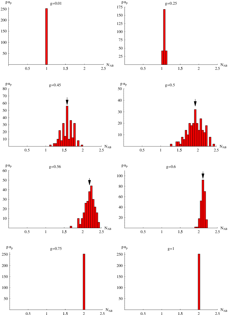
The distribution of the participation number $N_{AB}$ as $g$ varies, for $n=10$ qubits and $\epsilon=0$ , is shown in Fig. 1. We notice that the distribution is always well-behaved and bell-shaped, being practically a $\delta$ function for $g\leq 0.1$ and $g\geq 0.75$ . For this reason, one can get a satisfactory characterization of multipartite entanglement by looking at its mean value and width

\mu=\langle N_{AB}\rangle,\quad\sigma^{2}=\langle{(N_{AB}-\mu)}^{2}\rangle,

(9)

where the average $\langle\cdots\rangle$ is evaluated over all balanced bipartitions. We recall that $\mu$ defines the amount of entanglement while the inverse width $\sigma^{-1}$ describes how fairly such entanglement is distributed. We notice that the width $\sigma$ is maximum at $g=0.5$ , while the average entanglement $\mu$ is maximum at $g=0.56$ . Observe that no singularities can be expected for a number of spins as small as $n=10$ , yet the behavior of both quantities clearly foreruns the quantum phase transition at $g=g_{c}=1/2$ . In this sense, both $\sigma$ and $\mu$ appear to be good indicators of the QPT.

Refer to caption — Figure 1: Distribution function of the participation number $N_{AB}$ over all balanced bipartitions for the Hamiltonian (6) when $\epsilon=0$ and $n=10$ . The distribution is always bell-shaped. Its width is maximum at $g=0.5$ , while its average entanglement (indicated by a black arrow) is maximum at $g=0.56$ . Notice the different scales on the ordinates. The number of balanced bipartitions is $n_{p}=\left(\!\!\!\begin{array}[]{c}n\cr[n/2]\end{array}\!\!\!\right)=\left(\!\!\!\begin{array}[]{c}10\cr 5\end{array}\!\!\!\right)=252$ .

3.2 Average and width

Let us consider the full Hamiltonian (6) when the longitudinal perturbing field is small. In Fig. 2 we plot $\mu$ and $\sigma$ , respectively, vs $g$ for the ground state of the Hamiltonian (6), when $n=9$ , for different values of $\epsilon$ (ranging from $0$ to $10^{-2}$ ). We notice a very different behavior of the two quantities. The average $\mu$ is very sensitive to the longitudinal perturbation. In the region $g\simeq 1$ , where the ground state is approximately a GHZ state when $\epsilon=0$ , the average entanglement is strongly reduced even for a very small value of $\epsilon$ ( $\simeq 10^{-6}$ ). This is basically due to the fact that the superposition $|{\rm all\;spins\;up}\rangle+|{\rm all\;spins\;down}\rangle$ (yielding $\mu=2$ ) is very fragile and the ground state collapses in one of the two (degenerate) classical ground states (yielding $\mu=1$ ), the $Z_{2}$ symmetry being broken. On the other hand, near the maximum, $\mu$ is more robust and a larger perturbation ( $\epsilon=10^{-2}$ ) is required to counter larger values of $(1-g)$ and modify the behavior of $\mu$ .

The behavior of $\sigma$ is different. When $\epsilon\lesssim 10^{-2}$ the curves are not modified by the presence of the longitudinal field. This is due to the fact that in the region where $\mu$ is reduced by the presence of $\epsilon$ , $\sigma$ is already near to 0 (a GHZ state has $\sigma=0$ because it is invariant for permutation of the qubits, see [9]). Of course, a sufficiently large value of $\epsilon$ affects also $\sigma$ , reducing it (but not modifying the shape of $\sigma(g)$ ).

We shall now focus on the critical region. It would be tempting to take a small value of $\epsilon$ (say, $\epsilon=10^{-6}$ ) in order to get rid of the spurious residual entanglement at $g\simeq 1$ (and obtain a bell-shaped function for $\mu$ —as well as for $\sigma$ ). However, since we aim at a precise determination of the coordinates of the maximum, which is unaffected by small values of $\epsilon$ , we decided to work with $\epsilon=0$ .

3.3 Purely transverse Ising chain

In Fig. 3 we evaluate the average and standard deviation for $\epsilon=0$ (purely transverse) Ising chains of increasing size (from 7 to 11 sites). In Fig. 3(a) we distinguish different zones. For $g=0$ the ground state (gs) is factorized and $\mu=1$ . If $g\simeq 1$ the gs is approximately a GHZ state (a combination of the gs’s of the classical Hamiltonian). The most interesting region is around the value $g=0.5$ , where for an increasing number of qubits there is a more and more pronounced peak of $\mu$ . This is in qualitative agreement with other results obtained using the entropy of entanglement.

The width of the distribution of $N_{AB}$ versus $g$ is shown in Fig. 3(b). We will comment later on the behavior of this quantity, that yields useful additional information about the structure and generation of multipartite entanglement (information that would not be available for an entanglement measure constituted by a single number). Also in this case we can distinguish several regions in the plot. Moreover, the coupling $g$ corresponding to the peak of $\sigma$ (that we denote $\sigma_{\rm max}$ ), does not coincide with that corresponding to the peak of $\mu$ (that we denote $\mu_{\rm max}$ ):

g\left(\sigma_{\rm max}\right)<g\left(\mu_{\rm max}\right).

(10)

In other words, for a finite spin chain, the width of the distribution is not maximum when the amount of entanglement is maximum.

We notice that, by increasing $n$ , both maxima are shifted towards the center of the plot $g\to g_{\rm c}=0.5$ . In Fig. 4(a) we plot the values of the coupling constant $g$ at $\mu_{\rm max}$ versus the number of sites $n$ . The numerical result can be fitted with the (arbitrary) function

g(\mu_{\rm max})=0.5+\frac{5.43}{n^{2}+3.09\,n-35.59}\stackrel{{\scriptstyle n\to\infty}}{{\longrightarrow}}0.5=g_{c}.

(11)

The plot of $g(\sigma_{\rm max})$ versus $n$ is shown in Fig. 4(b), the fit being

g\left(\sigma_{\rm max}\right)=0.5+\frac{0.14}{n^{2}-13.01\,n+46.39}\stackrel{{\scriptstyle n\to\infty}}{{\longrightarrow}}0.5=g_{c}.

(12)

Notice that the fit (11) is very accurate, while (12) is valid within one standard deviation (namely a few percent), as can be seen in Fig. 4. From Fig. 4 and Eqs. (11)-(12) one can argue that the amount of entanglement (the mean of the distribution) and the maximum width of the distribution of bipartite entanglement can detect, in the limit of large $n$ , the QPT.

We shall henceforth focus on $\mu_{\rm max}$ and $\sigma(\mu_{\rm max})=\sigma(g(\mu_{\rm max}))$ (the value of $\sigma$ when the amount of entanglement is maximum), rather than $\sigma_{\rm max}$ (whose behavior is anyway similar). In Fig. 5 we plot these quantities vs the number of spins $n$ . They are fitted by (for $n\geq 6$ )

	$\displaystyle\mu_{\rm max}$	$\displaystyle=$	$\displaystyle 2+0.019\,\left(n-6\right)+0.007\,{\left(n-6\right)}^{2},$		(13)
	$\displaystyle\sigma(\mu_{\rm max})$	$\displaystyle=$	$\displaystyle-0.077+0.11\,{\sqrt{n-6}}.$		(14)

We also evaluate the relative width at maximum entanglement

\sigma_{\rm rel}=\sigma(\mu_{\rm max})/\mu_{\rm max},

(15)

shown in Fig. 6, that will be useful in the following discussion. The fitting curve in Fig. 6 is not independent, but is rather derived from Eqs. (13)-(14):

\sigma_{\rm rel}=\frac{-0.077+0.11\,{\sqrt{n-6}}}{2+0.019\,\left(n-6\right)+0.007\,{\left(n-6\right)}^{2}}.

(16)

4 Discussion

Both fits (13)-(14) imply that the entanglement indicators $\sigma$ and $\mu$ diverge with $n$ at the QPT. This conclusion is particularly significant: the amount of entanglement goes to infinity but so does the width of the entanglement distribution. In particular, this leads to two possible scenarios, depending on the behavior of $\sigma_{\rm rel}$ defined in (15):

1.

$\sigma_{\rm rel}\stackrel{{\scriptstyle n\rightarrow\infty}}{{\longrightarrow}}0$ . In this case the divergence of $\mu_{\rm max}$ is stronger than that of $\sigma(\mu_{\rm max})\simeq\sigma_{\mathrm{max}}$ . This means that at the QPT the entanglement of the ground state is macroscopically insensitive to the choice of the bipartition. Accordingly, the QPT yields a fair distribution of bipartite entanglement and is therefore a good tool for generating multipartite entanglement. This conclusion could pave the way towards a deeper understanding of the relation among entanglement, QPTs and chaotic systems (that are known to generate large amounts of entanglement [13, 18]).
2.

$\sigma_{\rm rel}\stackrel{{\scriptstyle n\rightarrow\infty}}{{\longrightarrow}}c>0\,\,(\mbox{eventually}\,\infty)$ . This situation would have profound consequences on our comprehension of the relation between a QPT and the generation of multipartite entanglement. In particular, the strong divergence of $\sigma(\mu_{\rm max})$ (of order equal to or larger than that of $\mu_{\rm max}$ ) would imply that the distribution of entanglement is not optimal, inasmuch as it is not fairly shared. This means that the amount of entanglement of non-contiguous spins partitions macroscopically differs from that of contiguous ones.

Our results, although not conclusive due to the relatively small value of $n$ reached in our numerical analysis, appear to indicate that (i) is the most probable scenario: indeed, from Eq. (16), that in turn is a consequence of Eqs. (13)-(14), we infer that for large $n$

\sigma_{\rm rel}\sim n^{-3/2}.

(17)

In general, if one assumes that the behavior of $\mu_{\rm max}$ and $\sigma(\mu_{\rm max})$ vs $n$ (and in particular the convexity of the two curves) does not change for larger $n$ , one can conclude that $\sigma_{\rm rel}$ vanishes for $n\to\infty$ .

Another important observation, related to the “entangling power” of evolutions [19], is the following. Although our numerical results seem to favor the first scenario, namely a well distributed multipartite entanglement generated by the quantum phase transition, such entanglement is not so large. Indeed, a typical $n$ -qubit state is characterized by [9]

\mu\propto 2^{n/2},\qquad\sigma=\mathrm{const},

(18)

namely an exponentially large amount of entanglement, that is also very well distributed. These typical states are efficiently produced by a chaotic dynamics [13, 18]. In general, one observes a very rapid growth of the (effective) Schmidt number (3) at the onset of chaos and for all these reasons, quantum chaos is a much better multipartite entanglement generator than a critical Ising chain. This conclusion seems to be valid for other spin Hamiltonians as well. Notice that the entangling power (and/or entanglement generation) of a QPT is better compared to that of a chaotic system [18] (in that they are both obtained by varying one or more coupling constants), rather than that of a quantum evolution [19]. On the other hand, unlike in a chaotic system, in a QPT one focuses on the features of the ground state.

The entanglement generation at a QPT and the physical features of this entanglement [20, 21] deserve additional investigations. The participation number or the entropy of entanglement (or any other sensible measure) are related to the global structure of the state. It is therefore reasonable to expect that many observables might be necessary in order to characterize multipartite entanglement. The approach we propose [9, 14], based on the calculation of the probability density function of bipartite entanglement, has the advantage of making use of statistical information on the state of the system and characterizes multipartite entanglement by extending techniques that are widely used in the analysis of its bipartite aspects. We have seen that when the density functions are well behaved and bell-shaped, the average and second moment of the distribution are good indicators of the quantum phase transition. These conclusions must be corroborated by the study of other systems and models displaying quantum phase transitions, as well as by the analysis of more complex systems [10, 11]. Work is in progress in this direction.

We thank A. Scardicchio and K. Yuasa for interesting remarks. This work is partly supported by the European Community through the Integrated Project EuroSQIP.

References

[1] S. Sachdev, “Quantum Phase Transitions”, Cambridge Univ. Press. (1999).
[2] A. Osterloh, L. Amico, G. Falci, and R. Fazio, Nature 416, 609 (2002).
[3] G. Vidal, J. I. Latorre, E. Rico, and A. Kitaev, Phys. Rev. Lett. 90, 227902 (2003).
[4] F. Verstraete, M. Popp, and J. I. Cirac, Phys. Rev. Lett. 92, 027901 (2004).
[5] T. Roscilde, P. Verrucchi, A. Fubini, S. Haas, and V. Tognetti, Phys. Rev. Lett. 93, 167203 (2004).
[6] W. K. Wootters, Quant. Inf. Comp. 1, 27 (2001); C. H. Bennett, D. P. DiVincenzo, J. A. Smolin, and W. K. Wootters, Phys. Rev. A 54, 3824 (1996).
[7] D. Bruss, J. Math. Phys. 43, 4237 (2002).
[8] V. Coffman, J. Kundu and W. K. Wootters, Phys. Rev. A 61, 052306 (2000); A. Wong and N. Christensen, Phys. Rev. A 63, 044301 (2001); D.A. Meyer and N.R. Wallach, J. Math. Phys. 43, 4273 (2002).
[9] P. Facchi, G. Florio and S. Pascazio, Phys. Rev. A 74, 042331 (2006).
[10] G. Parisi, “Statistical Field Theory” (Addison-Wesley, New York, 1988).
[11] V. I. Man’ko, G. Marmo, E. C. G. Sudarshan and F. Zaccaria J. Phys. A: Math. Gen. 35, 7137 (2002).
[12] E. Lubkin, J. Math. Phys. 19, 1028 (1978); S. Lloyd and H. Pagels, Ann. Phys., NY, 188, 186 (1988); K Życzkowski and H.-J. Sommers J. Phys. A 34, 7111 (2001); Y. Shimoni, D. Shapira and O. Biham, Phys. Rev. A 69, 062303 (2004).
[13] A. J. Scott and C. M. Caves, J. Math. Phys. 36, 9553 (2003).
[14] P. Facchi, G. Florio and S. Pascazio, “Charactering and measuring multitipartite entanglement”, quant-ph/0610108, International Journal of Quantum Information, in print.
[15] R. Grobe, K. Rza̧żewski and J.H. Eberly, J. Phys. B 27, L503 (1994).
[16] C. Tsallis, J. Stat. Phys. 52, 479 (1988).
[17] C. Holzhey, F. Larsen and F. Wilczek, Nucl. Phys. B 424 (1994) 443; C. Callan and F. Wilczek, Phys. Lett. B 333 (1994) 55; P. Calabrese and J. Cardy, J. Stat. Mech. P06002 (2004).
[18] J. N. Bandyopadhyay and A. Lakshminarayan Phys. Rev. Lett. 89 060402 (2002); S. Montangero, G. Benenti, and R. Fazio, Phys. Rev. Lett. 91, 187901 (2003); S. Bettelli and D. L. Shepelyansky, Phys. Rev. A 67, 054303 (2003); C. Mejìa-Monasterio, G. Benenti, G. G. Carlo, and G. Casati, Phys. Rev. A 71, 062324 (2005).
[19] P. Zanardi, Ch. Zalka, and L. Faoro, Phys. Rev. A 62, 030301 (2000).
[20] T. R. de Oliveira, G. Rigolin, M. C. de Oliveira, and E. Miranda, Phys. Rev. Lett. 97, 170401 (2006); T. R. de Oliveira, G. Rigolin, and M. C. de Oliveira, Phys. Rev. A 73, 010305 (2006).
[21] L. Campos Venuti, C. Degli Esposti Boschi, M. Roncaglia, and A. Scaramucci, Phys. Rev. A 73, 010303 (2006).