Single photon state generation from a continuous-wave non-degenerate optical parametric oscillator
Abstract
We present a theoretical treatment of conditional preparation of one-photon states from a continuous-wave non-degenerate optical parametric oscillator. We obtain an analytical expression for the output state Wigner function, and we maximize the one-photon state fidelity by varying the temporal mode function of the output state. We show that a higher production rate of high fidelity Fock states is obtained if we condition the outcome on dark intervals around trigger photo detection events.
pacs
03.65.Wj; 03.67.-a; 42.50.DvI Introduction
Light has come to play an important role in quantum information sciences, and this puts focus on the ability to prepare and manipulate state vectors of light, i.e., to restrict the field to a few modes or a single field mode, and to interact exclusively with the selected modes. In optical and microwave cavities, many experiments have already been done on pure quantum state manipulation in isolated field modes interacting with single atoms, but there is also an obvious interest to produce traveling light fields with controllable pure state properties.
It is not easy to manipulate quantum states of light, and one very successful strategy has thus been to produce a certain ”easy” state, and to use a quantum measurement to project this state on the desired quantum state. Following the theoretical proposals by Dakna et al dakna, see also sasaki; kim, conditioned on appropriate detection events, single- and two-mode squeezed states of light can be transformed into Fock states and Schrödinger cat-like states, as demonstrated with good fidelity with single mode pulses of light in lvovsky; zavatta; grangier2; grangiercat. I.e., a large number of pulses are generated, and measurements, carried out on each of them with some success probability, ascertain the preparation of the desired state.
A scheme to produce single photon states and other single mode quantum states from a continuous-wave field was demonstrated in experiments jonas; wakui, where a photon counter registered the intensity of a small fraction of a beam of squeezed light, causing the remaining beam to have a high single photon amplitude in a well localized mode. A theoretical analysis of that experiment was given in klaus. In the present paper we generalize the approach of klaus to protocols involving twin beams of light generated from a non-degenerate optical parametric oscillator (OPO). The non-degenerate OPO converts photons from a pump beam into pairs of photons in a pair of output modes, and a conditional detection of a single photon in one beam (which we shall denote the trigger beam) results in the presence of a single photon in the other beam (the signal beam). A possible experimental setup is sketched in figure 1. In contrast to the pulsed case where the field mode occupied is governed by the pulse shape, in the continuous-wave case, the precise temporal modes occupied by the one-photon states in the signal beam have to be specified. The largest one-photon state fidelities are obtained by choosing the modes optimally, and we present results of a variational procedure and of a numerical optimization.
In Sec. II, we introduce the quantum correlation functions of the twin beams of interest, and we show how the (Schrödinger picture) quantum state populating an arbitrary field mode can be readily obtained from the (Heisenberg picture) field correlation functions. In Sec. III, we present analytical results for the phase space Wigner function for the signal state conditioned on a single photo detection event and for the fidelity and rate with which the one-photon states are produced. In Sec. IV, we utilize a variational method to optimize the signal mode function. Finally, in Sec. V, we analyze the signal state conditioned on a photo detection event surrounded by an interval with no photo detection events. Sec. VI concludes the paper.

II Two-time quantum correlation functions and phase space Wigner functions for Gaussian states
The OPO Hamiltonian is quadratic in field annihilation and creation operators, and the solution of the time evolution is most easily accomplished by a linear (Bogoliubov) transformation of each pair of incident field operators at all frequency components. The state therefore retains the Gaussian state character of the vacuum state, i.e., the joint probability distributions of all the quadrature variables is Gaussian. The state separates in pairs of frequency modes for which the quantum state can be written down explicitly. Since we shall deal with photo detection experiments, we need a representation of the field in time domain, and although it is still a Gaussian state, it is now much more complicated, as the field operators at different times are non-trivially correlated.
In so-called Type I and Type II OPO’s, photons are created pairwise in two different frequency components and in two different polarization components, respectively. It is also possible to create photons pairwise in beams propagating in different directions. Alternatively one can combine the single beam squeezed light outputs from two degenerate OPO’s on a beam splitter, which also produce twin correlated beams, if the OPO outputs are squeezed out of phase. All of these approaches, if restricted to correlations in only one degree of freedom (polarization, frequency, direction), lead to quantum correlations described by the same formal correlation functions for the annihilation and creation operators for the two components, denoted in the following by and , , , , and , and are in quite precise models of the OPO’s given by drummond
| (1) |
where
| (2) |
The parameters in these expressions are the non-linear gain coefficient of the OPO, and the decay rate of light in the OPO cavity due to leakage through the output mirror. It is assumed that there is no loss through the other mirror. For fixed we note that is closely related to the mean twin beam intensity .
The modes relevant to the experiment are the mode , in which the trigger detection takes place, and the mode occupied by the produced state, while all other modes are unobserved. We assume the trigger detection to take place on a timescale much shorter than . The precise shape of the detected temporal mode is then irrelevant, and we assume
| (3) |
where is a short time interval and is the click time for the trigger detection. As discussed in the introduction, the mode function can be chosen arbitrarily (under the constraint ), and in particular it can be optimized to achieve maximal fidelity. The optimal mode function is centered around the trigger detector click time, and from (1) it is to be expected that the temporal extent is of order , which is the time that a photon can spend in the cavity and hence be separated from its partner in the output fields. We will return to this point in sections III and IV, but by now we leave unspecified. The problem thus reduces to the one of characterizing the correlations of the single mode operators
| (4) | |||||
| (5) |
where is the trigger detector efficiency, is the signal detector efficiency, and are field operators acting on vacuum, included to ensure appropriate commutator relations of and .
Since the state is Gaussian, we immediately know the multi-component Wigner function of the trigger and signal mode before conditioning on the trigger detector click event. Defining the column vector
| (6) |
of quadrature variables , this Wigner function is
| (7) |
is parameterized by the covariance matrix with elements , which are computed explicitly by use of equations (4) and (5), the time dependent mode functions , and the two-time correlation functions (1). Since it follows from (1) that , we have
| (8) | |||||
| (9) | |||||
| (10) | |||||
| (11) | |||||
| (12) |
We note that we use the same symbols for quadrature operators and for the corresponding real variable arguments in the Wigner function.
III Analysis of the state conditioned on the detection of a trigger photon
One can apply different trigger detector models taking into account the detailed physical functioning of the detector. In klaus, the theory is outlined for three such models: a perfect photon counter, an ”on/off” detector that discriminates vacuum from non-vacuum states, and a ”click” detector based on the absorption of a photon by the photoelectric effect. For general Gaussian states there are significant differences between the outcomes of these detector models, but as we are here interested in a trigger mode of infinitesimal duration and hence with vanishing populations of higher photon number states, they give identical results for the signal field state after the final state of the trigger mode is traced out. We henceforth apply the normal photo detector theory, where a click detection is accompanied by the application of the trigger field annihilation operator on the quantum state of the system, i.e., by application of the annihilation operator from the left and its adjoint creation operator from the right on the density matrix. Afterwards, the otherwise unobserved trigger mode is traced out.
The application of the annihilation and creation operations is mapped to differential operators on the Wigner function gardiner, and the partial trace is performed by an integration over the corresponding phase space variables. This results in the following Wigner function for the conditioned signal state
| (13) |
where is a normalization constant. By partial integration (13) reduces to
| (14) | |||||
where the coefficients , , and are given in terms of the covariance matrix elements (8-12)
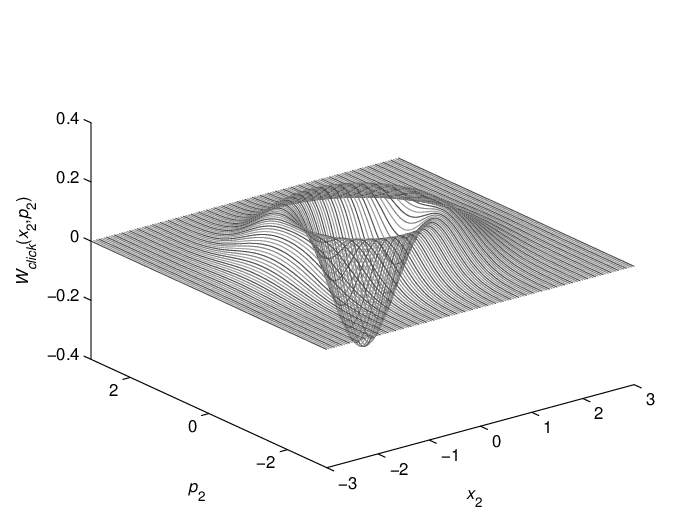
depends on the signal mode function , the signal detector efficiency , and the non-linear gain coefficient of the OPO through , but does not depend on the trigger detector efficiency . Since we condition on a click event, the only effect of an inefficient trigger detector is to reduce the production rate. Figure 2 shows for , , and (in the next section we prove that this is the optimal mode function for ). The fidelity, by which the conditioned Wigner function resembles the Wigner function for a one-photon state
| (15) |
is
| (16) |
and for the Wigner function in figure 2 we find .
For completeness we present in appendix A analytical results for the Wigner function and the one-photon state fidelity for the degenerate OPO setup analyzed in klaus.
The optimal signal mode function (denoted ) obtained from numerical optimization of the one-photon state fidelity (16) is shown in figure 3 for and different values of . (The optimization is over all real functions, which will be justified in the next section.) The tendency is that the width of the mode function decreases, when the beam intensity is increased, and a dip appears on each side of the peak. However, the difference between the optimal mode function for and for is quite small.

The optimized fidelity is shown in figure 4 for and (solid lines). The fidelity decreases with increasing because the two-photon state contribution to the output state increases when the intensity increases. The effect of reducing from 1 to 0.8 is roughly to reduce the fidelity by 20 % in the small region. For larger the reduction is smaller because the lower efficiency reduces the intensity seen by the detector. The dashed curves in the figure show the fidelity calculated for the mode function , and it is apparent that this analytical approximation is close to optimal for . This region is also the most interesting region since the fidelity is low for larger .

The production rate (i.e. the trigger detector click rate) is , where is the probability to observe a click in the trigger mode function. We assume that , which is valid if is small compared to the mean temporal distance between the photons in the trigger beam. The probability to observe a click in the trigger mode is then the expectation value of the number of photons in that mode, and hence
| (17) |
Figure 5 shows the production rate as a function of for . The rate decreases when decreases and is zero when . However, to achieve a high fidelity, needs to be small according to figure 4. Assuming perfect signal transmission, one-photon states with a fidelity of can be produced at rates of tens of kHz, if we assume and of order . These numbers are in quantitative accord with the experimental parameters and count rates for degenerate OPO’s jonas; wakui. In Sec. V we analyze the possibility to obtain better production rates and fidelities by conditioning on clicks surrounded by intervals with no click detection events, but first we consider the mode function optimization in greater detail.

IV Variational optimization of the signal mode function
In this section we optimize the signal mode function by analytical variation of the one-photon state fidelity (16). We write the signal mode function as , where is real. and may be varied independently, and since the constraint does not involve , the optimal choice of fulfils that the variation of vanishes, when is varied, which leads to
| (18) |
where
Note that and depend on the signal mode function through the covariance matrix elements, but they do not depend on time. Note also that and are both proportional to , while is independent of and .
For a general the solution to (18) is , where is an integer that may be different at different times. (18) is also fulfilled in the limit where varies infinitely fast with time, but this leads to and , and hence reduces to the Wigner function for vacuum and . Thus the phase is constant except for possible sign shifts. Adding a time independent constant to is equivalent to rotating the signal state Wigner function in phase space, but since the desired signal state Wigner function depends on and through , it is rotationally symmetric, and hence the fidelity is unchanged by this transformation. Consequently, we can choose , and it is thus sufficient to optimize over all real functions.
Restricting to be real, the constraint is , and this is taken into account by introducing a Lagrange multiplier and demanding the variation of to vanish when is varied. This leads to the following integral equation for the optimal signal mode function
| (19) |
For the first term in (19) vanishes, and we have
| (20) |
(20) is the optimal zero intensity signal mode function, and for the fidelity is . For , (20) can be used as the starting point for a numerical iteration of (19). To increase the range of values, where the iteration procedure converges, we use the mode function in the iteration step, where is the mode function obtained from the step. is a number between and , and is a normalization constant. Using this method we regain the mode functions in figure 3.
V Continuous detections with (efficient) trigger detector
In Sec. III we calculated the one-photon state fidelity for the output state conditioned on a single click event. Conditioning solely on one click event means that we average over all possible outcomes of the trigger detector measurements outside the small time window where the conditioning click occurs. This method is correct if the trigger detector is turned off outside the conditioning click time window, or if we want to calculate the average fidelity for a large number of produced states where no selection of particular click events (for instance those with no other clicks nearby) has taken place. However, an improvement in fidelity for fixed can be obtained if we only accept clicks that are surrounded by a certain time period with no clicks since this restricts the two-photon and higher photon number state contributions to the produced state. The fidelity increase depends on the trigger detector efficiency. If , it is certain that no photons hit the trigger detector during the period if no clicks are registered, and for large the fidelity approaches unity irrespective of the value of (provided is much smaller than the mean temporal distance between photons in the trigger beam). In the opposite limit, , a vacuum detection (i.e. no click) gives us no information about the produced state, and we regain the results from Sec. III.
For fixed the conditioning on a no click interval results in a smaller production rate because some clicks are now disregarded, but since the fidelity is increased, we can increase a little while still obtaining a larger fidelity than in Sec. III, and if is not too large, this leads to a larger production rate. In the region where the rate is limited by the number of photons produced by the source it thus turns out that an increase in production rate for fixed fidelity or an increase in fidelity for fixed production rate can be obtained.
In the following we first calculate the one-photon state fidelity for the signal state conditioned on one click detection and an arbitrary number of no click detections, and after that we derive an equation for the corresponding production rate. Finally we present and discuss numerical results for the fidelity and the production rate.
V.1 Fidelity
To determine the one-photon state fidelity for the produced state conditioned on a click event surrounded by a time interval with no click events, we replace the continuous time argument by a discrete set of box shaped temporal trigger mode functions and assume the trigger detections to take place in these modes. The vacuum detection modes are labeled by the numbers and are included in the covariance matrix. The unconditioned Wigner function is then
| (21) |
where . We first determine the Wigner function for the state conditioned on all the vacuum detections but not the click. A vacuum detection results in a projection of the relevant mode on the vacuum state, which in terms of Wigner functions corresponds to multiplication with the vacuum state Wigner function followed by integration over the relevant quadrature variables and renormalization. Thus the Wigner function for the state conditioned on the vacuum detections is
| (22) |
where is a normalization constant. Since the vacuum projection is a gaussian operation, is also a gaussian function. This means that we can proceed as in Sec. III if we just replace the covariance matrix for the output mode and the click mode with the covariance matrix corresponding to the gaussian Wigner function . If we write the covariance matrix for the signal mode, the click mode, and the vacuum modes as
| (23) |
where is the covariance matrix for the signal mode and the click mode, and is the covariance matrix for the vacuum modes, it has been proven eisert that
| (24) |
where is the identity matrix. Hence by use of (24) we can immediately calculate the improved fidelity from (16) (note that the covariance matrix elements that are equal in Sec. III are changed by equal amounts and are hence still equal).
V.2 Production rate
The production rate is
| (25) |
where is the probability to detect no click in the vacuum modes and a click in the click mode. To determine we calculate the overlap of the unconditioned source output state with the vacuum state in the vacuum modes and then the expectation value of in the click mode
| (26) |
Since we consider trigger modes only, the signal mode is not included in the covariance matrix in (26). Performing the integration we find
| (27) |
where we have introduced the following notation: is the identity matrix, is a matrix with elements for and otherwise, is the matrix consisting of all the odd-odd matrix elements of , is an matrix with elements for and otherwise, and means that the first row and the first column of the matrix (corresponding to the click mode) have been removed.
V.3 Numerical results
In all the numerical calculations in this subsection and . For (and ) we find , and hence the assumption is valid for the region, where the fidelity is large. Even for , is still somewhat smaller than .

Figure 6 shows the optimized one-photon state fidelity as a function of the time interval in which we demand no click events to occur. is chosen symmetrically around the trigger detector click time, i.e. we condition on no clicks from to and from to , since this gives rise to the largest fidelity increase for a given . The rate and fidelity expressions are, however, also valid for asymmetrical time intervals (and even for time intervals interrupted with periods where the trigger detector is turned off). As expected the fidelity increases when increases if , and for the fidelity approaches one for large . For a moderate trigger detector efficiency , the fidelity increase is smaller, but still significant. The fidelity increase levels off when increases beyond approximately irrespective of the value of . The reason for this is that the temporal extent of the signal mode function is approximately as is apparent from figure 7, which shows the optimal signal mode function for , , and different trigger detector efficiencies. For the mode function is identical to the mode function in figure 3, but when is increased to non-zero values, the mode function approaches the optimal mode function (20) (the dot-dashed line in the figure).


The optimized one-photon fidelity as a function of for and different values of trigger detector efficiency is plotted in figure 8. The dashed curve () is identical to the curve in Sec. III, so the difference between the solid line and the dashed curve shows the fidelity increase when increases from 0 to 10 for . increases with because the mean temporal distance between the photons in the trigger and the signal beam decreases when increases, and hence it is more likely to have close clicks. The dotted curve in the figure is for perfect trigger detection , and as expected it is close to unity for all .

The production rates corresponding to the solid line and the dotted line in figure 8 are shown in figure 9, and the dashed line in figure 9 is the rate for and . The production rate vanishes for zero intensity because there are no photons present in the trigger beam in that limit. Also in the large intensity limit the rate approaches zero for . The reason is that the large photon flux makes it extremely unlikely to observe no clicks during some non-zero time interval. It is desirable to be on the left side of the maximum of the relevant curve in figure 9 because the fidelity is a decreasing function of . Hence for and , should be below 0.20, while for , should be below 0.28. The curve is shifted to the right compared to the curve because a lower detector efficiency corresponds to a lower photon flux in the beam. The maximal rate ( for both curves) corresponds to a mean temporal distance between accepted clicks of . For the high fidelity region is . For this region it is apparent from figure 9 that the decrease in production rate for fixed is quite small when is increased from 0 to 10, while figure 8 shows that the fidelity increase is significant.
VI Conclusion
In conclusion we have considered conditional single photon state generation from a continuous-wave non-degenerate OPO. We have presented explicit analytical expressions for the output state Wigner function, the one-photon state fidelity, the production rate, and the optimal zero intensity limit temporal mode function for the signal state. We have optimized the mode function numerically to achieve maximal fidelity, and from a variational calculation we determined an integral equation for the optimal mode function. By conditioning on clicks surrounded by an interval with no clicks, the fidelity was increased for fixed , while the production rate was decreased slightly. However, accepting a smaller fidelity increase by increasing led to a larger production rate if and were not too large.
Using our approach, it is possible analytically to calculate the output state Wigner function conditioned on arbitrary sequences of click detections, vacuum (i.e. no click) detections, and no detections (i.e. detector turned off) in temporal trigger modes of short duration, and the corresponding production rate can also be determined analytically since both calculations involve integration of products of polynomials and Gaussian functions only. From the conditioned output state Wigner function it is straightforward to compute the fidelity for arbitrary states in arbitrary output modes. We are currently working on a generalization of our calculations for the production of single photon states to generation of -photon and Schrödinger kitten states.
The authors acknowledge discussions with Jonas S. Neergaard-Nielsen and Eugene S. Polzik, and financial support from the European Union through the Integrated Project ”SCALA”.
Appendix A Wigner function and fidelity for one-photon states produced from a degenerate OPO
The setup analyzed in klaus is obtained from figure 1 by replacing the non-degenerate OPO with a degenerate OPO and the polarizing beam splitter with a normal beam splitter with low transmission. The two-time correlation functions for this setup are klaus
| (28) | |||||
| (29) |
and (4) and (5) are modified to
| (30) | |||||
| (31) | |||||
where is the beam splitter reflectivity, and the operators labeled by are field operators acting on vacuum. As in Sec. IV we can restrict our analysis to real signal mode functions. In terms of the covariance matrix elements computed from (28), (29), (30), and (31) the Wigner function for the produced state conditioned on a single trigger detector click event is
| (32) |
where
and the one-photon state fidelity is
| (33) |
References
- (1) M. Dakna, T. Anhut, T. Opatrný, L. Knöll, and D.-G. Welsch, Phys. Rev. A 55, 3184 (1997).
- (2) M. Sasaki and S. Suzuki, Phys. Rev. A 73, 043807 (2006).
- (3) M. S. Kim, E. Park, P. L. Knight, and H. Jeong, Phys. Rev. A 71, 043805 (2005).
- (4) A. I. Lvovsky, H. Hansen, T. Aichele, O. Benson, J. Mlynek, and S. Schiller, Phys. Rev. Lett. 87, 050402 (2001).
- (5) A. Zavatta, S. Viciani, and M. Bellini, Phys. Rev. A 70, 053821 (2004).
- (6) A. Ourjoumtsev, R. Tualle-Brouri, and P. Grangier, Phys. Rev. Lett. 96, 213601 (2006).
- (7) A. Ourjoumtsev, R. Tualle-Brouri, J. Laurat, and P. Grangier, Science 312, 83 (2006).
- (8) J. S. Neergaard-Nielsen, B. M. Nielsen, C. Hettich, K. Mølmer, and E. S. Polzik, Phys. Rev. Lett. 97, 083604 (2006).
- (9) K. Wakui, H. Takahashi, A. Furusawa, and M. Sasaki, quant-ph/0609153.
- (10) K. Mølmer, Phys. Rev. A 73, 063804 (2006).
- (11) P. D. Drummond and M. D. Reid, Phys. Rev. A 41, 3930 (1990).
- (12) C. W. Gardiner and P. Zoller, Quantum Noise, Springer-Verlag, Berlin, 2000.
- (13) J. Eisert and M. B. Plenio, Int. J. Quant. Inf. 1, 479 (2003), quant-ph/0312071.