Robustness against parametric noise of non ideal holonomic gates

Cosmo Lupo Affiliation: Università di Napoli “Federico II” and INFN, Sezione di Napoli, via Cintia I-80126 Napoli, Italy Paolo Aniello Affiliation: Università di Napoli “Federico II” and INFN, Sezione di Napoli, via Cintia I-80126 Napoli, Italy Mario Napolitano Affiliation: Università di Napoli “Federico II” and INFN, Sezione di Napoli, via Cintia I-80126 Napoli, Italy Giuseppe Florio Affiliation: Università di Bari and INFN, Sezione di Bari, I-70125 Bari, Italy

Abstract

Holonomic gates for quantum computation are commonly considered to be robust against certain kinds of parametric noise, the very motivation of this robustness being the geometric character of the transformation achieved in the adiabatic limit. On the other hand, the effects of decoherence are expected to become more and more relevant when the adiabatic limit is approached. Starting from the system described by Florio et al. [Phys. Rev. A 73, 022327 (2006)], here we discuss the behavior of non ideal holonomic gates at finite operational time, i.e., far before the adiabatic limit is reached. We have considered several models of parametric noise and studied the robustness of finite time gates. The obtained results suggest that the finite time gates present some effects of cancellation of the perturbations introduced by the noise which mimic the geometrical cancellation effect of standard holonomic gates. Nevertheless, a careful analysis of the results leads to the conclusion that these effects are related to a dynamical instead of geometrical feature.

pacs

03.67.Lx, 03.65.Vf, 03.65.Yz

I Introduction

One of the most important challenges for the realization of quantum information tasks is the implementation of quantum logic gates that are robust against unwanted perturbations Nielsen_Chuang; Casati. Two kinds of perturbations with qualitatively different features can be distinguished: the first kind has a purely quantum nature, and it is induced by the interaction of the quantum system implementing the logic gate with the environment; the second kind has instead a classical nature, and it is caused by the presence of instrumental noise in the ‘external parameters’ used to control the system. The unwanted interaction with the environment is the source of the phenomenon known as quantum decoherence Breuer. The effects of this interaction can be modeled by means of suitable ‘master equations’ (i.e. evolution equations) for the density matrix of the quantum system implementing the logic gate; at least in the Markovian regime ¹¹ 1 It is worth stressing that in the limit for the operational time tending to zero the Markovian approximation cannot be applied, in principle — see, for instance, nonMarkov — and one cannot claim, in general, that environmental noise can be avoided by simply decreasing the operational time., they are negligibly small if the operational time of the logic gate is short enough. The classical perturbations stem from an unavoidable noisy component intrinsic in the external driving fields (e.g. laser beams NIST) that can be usually regarded as classical fields; hence, it is essentially due to instrumental instability. The effects of these perturbations can be evaluated by studying standard (non-autonomous) Schrödinger equations where the instrumental noise is taken into account by suitably modeling the noisy components of the classical parameters (e.g. the field amplitude) associated with the external driving fields.

Among the several strategies for realizing quantum logic gates discussed in the literature, a prominent position is held by holonomic gates. They were first proposed by Zanardi and Rasetti Zanardi_Rasetti (see also Ref. PachosPRA61), and rely on the theory of holonomy and of the associated holonomy groups in principal fiber bundles Nakahara, a subject which is familiar to theoretical physicists due to the central role played in gauge theories Marathe and in the well-known phenomenon of abelian Berry and non-abelian WZ adiabatic phases. Actually, a holonomic gate can be regarded as a straightforward application of the theory of non-abelian adiabatic phases to quantum computation.

Since the very beginning, holonomic gates were considered to be intrinsically robust against classical noise Pachos, thanks to the geometric features of holonomy in Hilbert bundles. As we will briefly recall below, three main ingredients are needed in order to realize such holonomic gates.
The first ingredient is a suitable physical system described by a quantum Hamiltonian depending on some set of parameters, these parameters being associated with the external (classical) driving fields that are assumed to be experimentally controllable functions of time; the unavoidable instrumental instability (stochastic noise) affecting the driving fields is the source of the classical noise — we will call it parametric noise, in the following — that has been mentioned above.
The second ingredient consists in selecting a suitable eigenspace of the given Hamiltonian — an eigenspace depending smoothly on the external parameters, hence actually an iso-degenerate family of eigenspaces; let us call them the family of relevant eigenspaces — and in fixing in the parameter space an ‘initial point’ and a loop through this point. To such a loop corresponds an excursion of the parameter-dependent Hamiltonian (hence, of its eigenprojectors) and a certain ideal unitary transformation in the encoding eigenspace, namely, that particular relevant eigenspace fixed by the initial (and final) point of the loop in the parameter space. This ideal transformation is determined by Kato’s adiabatic evolutor associated with the given Hamiltonian and with the chosen loop in the parameter space, and it has a simple geometric interpretation as a holonomy phenomenon (geometric phase). The ideal unitary transformation plays a central role in Kato’s formulation of the adiabatic theorem Kato applied to our context. Indeed, the external parameters are controllable functions of time and in the adiabatic limit — i.e., in the limit where the loop in the parameter space is covered in a operational time tending to infinity — the real evolution over the operational time, determined by the given physical Hamiltonian, becomes cyclic in the encoding eigenspace and, apart from an irrelevant overall ‘dynamical phase factor’, coalesces in this subspace with the ideal unitary transformation. We stress that the ideal unitary transformation should be thought, in our context, as an ideal quantum gate whose behavior can be, in general, only approached by a non-ideal quantum gate corresponding to the real evolution over a suitably large, but finite, operational time.
Accordingly, the third ingredient is the choice of a suitable operational time — which will be called balanced working time, in the following --- for the real quantum gate. This time span must be short enough to achieve a fast quantum computer and to avoid the ravages of decoherence, but long enough to justify the adiabatic approximation (i.e. to approach the behavior of the ideal quantum gate) which is at the root of the appearing of geometric phases ²² 2 We recall that geometric phases arise also in the context of (non-adiabatic) cyclic evolutions Aharonov; Anandan, but only adiabatic phases are relevant for our purposes.. Hence, a balanced working time is determined by a touchy trade-off between two competing and not necessarily compatible demands.

The problem of robustness of holonomic gates against parametric noise has been studied in both the abelian and non-abelian case with different approaches DeChiara_Palma; Solinas_Zanardi; Zu_Zanardi. In these papers, the effects of random perturbations of the control parameters are considered. It is worth noticing, however, that such effects are evaluated with the adiabatic limit already being performed, thus essentially confirming quantitatively the standard qualitative geometric argument usually adopted to support the robustness of holonomic gates, argument which will be recalled later on.

As holonomic gates are generally considered to be a priori robust against parametric noise, attention has mainly focused on the study of decoherence effects Carollo; Carollo2; Fuentes; Parodi and on the possibility of partially suppressing them Wu_Zanardi_Lidar. These investigations show that, for certain physical systems and for certain models and regimes of the coupling with the environment, one is able to estimate the typical time-scale within which the effects of decoherence can be neglected. Hence one can determine, in principle, a balanced working time for these systems. At this point one should actually check whether this balanced working time guarantees a suitable robustness of the quantum gate against parametric noise, namely, whether the effects of this kind of noise on the fidelity of the non-ideal quantum gate with respect to the ideal one can be neglected or not.

Recently, a new ingredient has been proposed for the implementation of a holonomic quantum gate Florio_1 (see also Florio_2; Florio_3) where the authors have observed — for the model of a ion-trap quantum gate proposed by Duan et al. Cirac — the existence of a optimal working time, namely, of a specific operational time for which the non-ideal (i.e. finite-time) gate behaves exactly as the ideal (i.e. adiabatic) gate; they show, furthermore, that over the optimal working time the effects of the environment are negligible. Thus, such a optimal working time turns out to be also a balanced working time.
We stress that, anyway, the fact that the non-ideal gate behaves, in correspondence to the optimal working time, as the ideal one cannot be used to rule out the influence of parametric noise on the base of the standard geometric argument. Indeed, one should not expect that, perturbing the loop in the parameter space, the non-ideal gate will still mimic the behavior of the ideal one. Hence one cannot apply, in principle, the standard geometric argument to support the robustness of this kind of holonomic gate against parametric noise. A critical analysis of this simple, but somehow subtle, issue is the main aim of the present contribution.

In conclusion, we think that the impact of parametric noise on holonomic gates is still an open problem and one is not legitimated, in general, to state the robustness of non-ideal holonomic gates against this kind of perturbations on the base a generic geometric argument. In our present contribution, we will try to illustrate this assertion by means of quantitative arguments, focusing on the ion-trap model proposed by Duan et al. Cirac. Even if other models have been proposed in the literature Falci, the model of Duan et al. is probably the one most extensively studied also with reference to different physical systems, as Josephson junctions Faoro and semiconductor quantum dots Solinas, and can be regarded as a reference point for the subject.

The paper is organized as follows. In Sec. II the model Hamiltonian is introduced which will serve as a case study. In Sec. III the behavior of the considered system in presence of several models of parametric noise is discussed. In Sec. IV the obtained results are analyzed and commented. Conclusions and remarks are presented in Sec. V.

II A case study

As a case study, here we consider the single-qubit non Abelian gate that was proposed in Cirac. The model under consideration can be physically realized as, for instance, a trapped ion with two degenerate ground (or metastable) states $|0\rangle$ and $|1\rangle$ which play the role of the computational basis. A quasi degenerate ancillary state $|a\rangle$ and an excited state $|e\rangle$ are also needed (the scheme is drawn in Fig. 1(a)). The low energy states are supposed to be independently coupled with the excited state, such that the interaction picture Hamiltonian in the rotating frame reads as follows:

H(\mathbf{r})=H(x,y,z)=|e\rangle\left[x\langle 0|+y\langle 1|+z\langle a|\right]+\mathrm{h.c.}\;.

(1)

The, in general complex, parameters $x,y,z$ are related to three independent Rabi frequencies corresponding to, in general de-tuned, laser beams with different energies and polarization. In an ideal experiment, however, the laser beams are assumed to be resonant with the corresponding transitions and the parameters are constrained to take values on a two-sphere. It is thus convenient to introduce polar coordinates:

\displaystyle\left\{\begin{array}[]{ccc}x&=&\Omega\sin{\vartheta}\cos{\varphi}\\ y&=&\Omega\sin{\vartheta}\sin{\varphi}\\ z&=&\Omega\cos{\vartheta}\end{array}\right.\;.

The spectrum of (1) is threefold: $\sigma=\{0,\pm\Omega\}$ , with the null eigenvalue which is doubly degenerate. The two degenerate eigenstates with vanishing energy can be chosen as follows:

\begin{split}|\psi_{0}\rangle&=\cos{\vartheta}\left(\cos{\varphi}|0\rangle+\sin{\varphi}|1\rangle\right)-\sin{\vartheta}|a\rangle,\\ |\psi_{1}\rangle&=-\sin{\varphi}|0\rangle+\cos{\varphi}|1\rangle.\end{split}

(6)

An analysis of the holonomy associated to the Hamiltonian (1) in correspondence with the doubly degenerate subspace shows that a closed path with starting point $\vartheta=0$ corresponds to a non Abelian holonomy $W=\exp{\left[-i\sigma_{y}\omega\right]}$ , where $\sigma_{y}=-i\left(|0\rangle\langle 1|-|1\rangle\langle 0|\right)$ is the Pauli matrix in the computational space and $\omega$ is the solid angle spanned by the parameter $\vartheta(s)$ and $\varphi(s)$ . This geometric character of the dynamics in the adiabatic limit is at the heart of the usual argument in favor of the robustness of holonomic quantum computation. A stochastic noise in the control parameter can modify the details of the loop but, for a sufficiently great number of cycles of the noise during the system evolution, the fluctuations in the swept solid angle are consider to become negligible (see DeChiara_Palma; Solinas_Zanardi and references therein).

Here we consider the closed path in the parameter manifold that was studied in Florio_1. For $s\in[0,1]$ we take (see Fig. 1(b)):

\begin{split}\vartheta(s)=&\left\{\begin{array}[]{ll}3s\pi/2&s\in[0,1/3]\\ \pi/2&s\in[1/3,2/3]\\ 3\pi/2\left(1-s\right)&s\in[2/3,1]\end{array}\right.\\ \varphi(s)=&\left\{\begin{array}[]{ll}0&s\in[0,1/3]\\ 3\pi/2\left(s-\frac{1}{3}\right)&s\in[1/3,2/3]\\ \pi/2&s\in[2/3,1]\end{array}\right.\end{split}

(7)

Refer to caption — Figure 1: Structure of the atomic levels and resonant lasers (a); unperturbed loop (7) in the parameter manifold (b).

The solid angle related to the loop (7) is $\omega=\pi/2$ , hence the corresponding holonomic gate is $W=-i\sigma_{y}$ . As was observed in Florio_1, the remarkable property of this path is that it presents perfect revivals of the gate fidelity at finite operational time. The same behavior was predicted for all the loops constructed by moving from the north pole to the equator through a meridian and back to the north pole through another meridian with piecewise constant velocity. In the case of the loop (7) there is a perfect revival of fidelity in correspondence of the operational times:

\tau^{*}_{k}=\frac{3\pi}{2\Omega}\sqrt{16k^{2}-1},\ \ k=1,2,\dots

(8)

In the following we are mostly concerned with the first optimal operational time $\tau^{*}_{1}$ .

To conclude this section we notice that a geometric phase appears in correspondence to a non adiabatic cyclic dynamics Aharonov; Anandan. In particular, for our case study, it happens that, in correspondence to an optimal operational time, the evolution becomes cyclic and the acquired geometric phase is equal to the adiabatic holonomy.

III Models of noise

In order to study the robustness of non ideal holonomic gates, we consider the response of the system under parametric noise in the ideal loop (7). In order to quantify the robustness of the gate, the noisy finite time evolution of the system is solved with analytic or numerical methods and the average gate fidelity is calculated. In the following, several models of noise are taken into account: in Sec. III.1 we consider the response of the system under a monochromatic perturbation of the three Rabi frequencies in (1); in Sec. III.2 we consider a model of noise expressed by a random step function in the angular variables (II) on the sphere; finally, in Sec. III.3 we discuss the response of the system under a random perturbation in the three Rabi frequencies.

III.1 Monochromatic perturbation

In this section we consider the behavior of the system in presence of a small perturbation in the parameters which can be viewed as a probe function used to test the stability of the gate, in particular we concentrate our attention to the case of a monochromatic probe function. A generic noisy path can be written as follows:

\mathbf{r}_{\mathrm{n}}(t)=\mathbf{r}(t)+\boldsymbol{\epsilon}(t),\ \ t\in[0,\tau],

(9)

where the vector $\mathbf{r}(t)$ describes the unperturbed loop and $\boldsymbol{\epsilon}(t)$ is a three component vector including the perturbation of the path. We have chosen a monochromatic perturbation at frequency $\eta$ and considered a noisy path obtained from (II) and (7):

\displaystyle\left\{\begin{array}[]{ccc}x_{\mathrm{n}}(s;\eta,\epsilon_{\eta},\tau,\phi_{1})&=&x(s)+\epsilon_{\eta}e^{i\eta\tau s+i\phi_{1}}\\ y_{\mathrm{n}}(s;\eta,\epsilon_{\eta},\tau,\phi_{2})&=&y(s)+\epsilon_{\eta}e^{i\eta\tau s+i\phi_{2}}\\ z_{\mathrm{n}}(s;\eta,\epsilon_{\eta},\tau,\phi_{3})&=&z(s)+\epsilon_{\eta}e^{i\eta\tau s+i\phi_{3}}\end{array}\right.\;,

where $\mathbf{r}_{\mathrm{n}}(s)\equiv(x_{\mathrm{n}}(s),y_{\mathrm{n}}(s),z_{\mathrm{n}}(s))$ , ${\boldsymbol{\phi}}\equiv(\phi_{1},\phi_{2},\phi_{3})$ are random phases uniformly distributed in $[0,2\pi)$ and $\epsilon_{\eta}$ is the strength of the noise (chosen to be equal for the three component). Notice that this model of noise acts on both the amplitude and the de-tuning of the lasers. From (III.1) it is clear that at finite operational time the perturbation does not reduces to a geometric perturbation of the loop in the parameters space since the perturbed path itself depends on the operational time. In presence of noise, different values of the operational time $\tau$ correspond to different loops in the parameters manifold.

For given values of $\eta,\epsilon_{\eta},\tau$ and $\boldsymbol{\phi}$ , we consider the solution of the Schrödinger equation

V_{\tau}^{\prime}(s;\eta,\epsilon_{\eta},\boldsymbol{\phi})=-i\tau H(\mathbf{r}_{\mathrm{n}}(s))V_{\tau}(s;\eta,\epsilon_{\eta},\boldsymbol{\phi}),\ \ s\in[0,1].

(14)

where, in presence of noise, the re-scaled Hamiltonian $H(\mathbf{r}_{\mathrm{n}}(s))$ depends on $\tau$ too. Since we are mainly interested in the transformation emerging at the end of the loop, we set $V_{\tau}(\eta,\epsilon_{\eta},\boldsymbol{\phi})\equiv V_{\tau}(1;\eta,\epsilon_{\eta},\boldsymbol{\phi})$ .

Notice that, for all practical purposes, taking the average on the random phases corresponds to the action of the completely positive map

\rho\longrightarrow\mathcal{E}(\rho)=\frac{1}{(2\pi)^{3}}\int d{\boldsymbol{\phi}}V_{\tau}(\eta,\epsilon_{\eta},\boldsymbol{\phi})\rho V_{\tau}(\eta,\epsilon_{\eta},\boldsymbol{\phi})^{\dagger}\;.

(15)

This completely positive map has to be compared with the ideal adiabatic unitary dynamics, to do that, we have evaluated the average gate fidelity

F=\int d\psi\langle\psi|W^{\dagger}\mathcal{E}(|\psi\rangle\langle\psi|)W|\psi\rangle\;,

(16)

where $d\psi$ indicates the normalized Fubini-Studi metric on pure states. This has been computed by means of the formula (see Ref. Nielsen):

F=\frac{1}{3}+\frac{1}{12}\mathrm{tr}\left[WW^{\dagger}\mathcal{E}(P_{0}(0))\right]+\frac{1}{12}\sum_{j=1}^{3}\mathrm{tr}\left[W\sigma_{j}W^{\dagger}\mathcal{E}(\sigma_{j})\right]

(17)

where $\sigma_{j}$ are the Pauli matrices in the computational subspace.

For several values of $\eta,\epsilon_{\eta}$ and $\boldsymbol{\phi}$ , Eq. (14) is numerically solved using the relation:

V_{\tau}(\eta,\epsilon_{\eta},\boldsymbol{\phi})=\lim_{N\rightarrow\infty}\stackrel{{\scriptstyle\leftarrow}}{{\prod}}_{k=0\dots N}\mathrm{exp}\left[-i\tau H(\mathbf{r}_{\mathrm{n}}(k/N))\frac{1}{N}\right]

(18)

Where $\overleftarrow{\prod}$ stands for the path ordered product. The effective completely positive map (15) is evaluated taking the average over $50$ random choices of the phases $\boldsymbol{\phi}$ .

Figure 2 shows the estimated gate fidelity (17) plotted as a function of the adimensional operational time $\Omega\tau$ , for several values of the noise amplitude and frequency. The unperturbed dynamics corresponds to $\epsilon_{\eta}=0$ and can be compared with the analytical results in Florio_1, it exhibits perfect revivals of the average gate fidelity at finite time, in particular the first optimal operational time is $\Omega\tau^{*}_{1}\simeq 18.25$ . The numerical results show that the pattern of gate fidelity as a function of the operational time can be completely different in presence of noise.

The average gate fidelity at the first optimal operational time $\tau^{*}_{1}$ in presence of parametric noise is plotted in Fig. 3 as a function of both amplitude and frequency of the noise. This plot suggests that the gate is indeed robust also for rather large noise amplitude ( $\epsilon_{\eta}=0.4\Omega$ ). It is worth to notice that this is true unless the perturbation frequency is in a particular range approximatively about $\eta\simeq 0.15\Omega$ . The presence of a typical frequency scale in the pattern of the fidelity is a feature that will be reencountered in the other models of noise considered below.

We have also studied, with the same methods, the response of the system in presence of analogous perturbations which have different symmetries. We have considered the case in which only the real part of (III.1) is taken; in this case the perturbation acts only in the amplitude of the coupling but not in the de-tuning. We have also analyzed the case of a perturbation which is square wave shaped; in this case a probe function is identified by its half period and initial phase. In both cases the corresponding patterns of the average gate fidelity are exactly analogous to the one shown in Fig. 3. This leads to the conclusion that the pattern of fidelity is largely independent of the details of the chosen probe function and a rather general behavior as function of the typical frequency is observed.

Analogous results are also found for other loops of the same kind, such as the loop with the angle $\varphi$ varying from $0$ to $\pi/4$ in (7) which is related to the Hadamard gate.

III.2 Random noise on the sphere

In this section we consider a model of noise which preserves the spectrum of the unperturbed Hamiltonian (1), because of its symmetries an analytical solution of the noisy dynamics is available.

In Florio_1 it was shown that the evolution operator can be evaluated without approximation in several situations. Referring to the model in Eq. (1), it is possible to evaluate the evolution operator along any segment on the parametric sphere as far as one of the parameters $(\vartheta,\varphi)$ is kept constant. In particular, referring to the case in Fig. 1(b), the loop is composed by three segments and along each of them the previous condition is satisfied. Thus one can demonstrate Florio_1 that the total evolution operator can be splitted in the form

U(\tau)=U_{3}(\tau_{3})\,U_{2}(\tau_{2})\,U_{1}(\tau_{1}),

(19)

where $\tau$ is the total time evolution and $\tau_{i},\,i=1,2,3$ are the times needed for covering each segment (for simplicity we suppose that the speed of the evolution are constant in each segment); moreover, the intermediate $U_{i}$ ’s can be explicitly calculated Florio_1. Their form is very peculiar and it is possible to see that, in terms of the parameters $(\vartheta,\varphi)$ , one can write

$\displaystyle U_{1}(t_{1})$	$\displaystyle=$	$\displaystyle U_{1}(\vartheta_{1}(t_{1}),\varphi_{1}),$	(20)
$\displaystyle U_{2}(t_{2})$	$\displaystyle=$	$\displaystyle U_{2}(\vartheta_{2},\varphi_{2}(t_{2})),$	(21)
$\displaystyle U_{3}(t_{3})$	$\displaystyle=$	$\displaystyle U_{3}(\vartheta_{3}(t_{3}),\varphi_{3}),$	(22)

where $0\leq t_{i}\leq\tau_{i}$ and $\varphi_{1}$ , $\vartheta_{2}$ and $\varphi_{3}$ are the constant values of the parameters during the evolution along the segment $1$ , $2$ and $3$ respectively.

We want to use these results for gaining information about the influence of the noise. We will therefore consider the following model: every $U_{i}$ is splitted in $N$ evolution operators $U_{i}^{j}$ evolving for a time $\tau_{\text{step}}$ (a sub-segment) such that

N=\tau_{i}/\tau_{\text{step}}.

(23)

The evolution in the segment $i$ reads

U_{i}(\tau_{i})=\prod_{j=1}^{N}U_{i}^{j}(\tau_{\text{step}}).

(24)

In each sub-segment one of the sphere parameters is constant and the other evolves (we are moving on meridians or parallels). We add a random component to the constant parameter while the other is not affected. In other words, we are including a transverse component. We also suppose that the transverse evolution operator is equal to the identity (the “switch” is infinitely fast). This way we have splitted the evolution on a single meridian (parallel) in a sequence of evolutions of shorter meridians (parallels). Using Eq.s (20)-(24) we can write

	$\displaystyle U_{1}(\tau_{1})=\prod_{j=1}^{N}U_{1}^{j}(\vartheta_{1}(t_{1}^{j}),\varphi_{1}+\xi_{1}^{j}),$		(25)
	$\displaystyle U_{2}(\tau_{2})=\prod_{j=1}^{N}U_{2}^{j}(\vartheta_{2}+\xi_{2}^{j},\varphi_{2}(t_{2}^{j})),$		(26)
	$\displaystyle U_{3}(\tau_{3})=\prod_{j=1}^{N}U_{3}^{j}(\vartheta_{3}(t_{3}^{j}),\varphi_{3}+\xi_{3}^{j}),$		(27)

where $(j-1)\tau_{\text{step}}\leq t_{i}^{j}\leq j\tau_{\text{step}}$ and $\xi_{i}^{j}\in[-\gamma,\gamma]$ are random variables uniformly distributed in the chosen interval ( $i=1,2,3$ ). We stress again that each operator in the decomposition has a (large and not transparent) analytical expression. Using this model we have computed the average gate fidelity at the first optimal operational time $\tau^{*}_{1}$ by means of Eq. (17) (and averaged over $50$ realizations of the random process). The result is shown in Fig. 4; $F$ is plotted as a function of the noise amplitude $\gamma$ (re-scaled with the maximum value of the parameter for the loop in Fig. 1(b) i.e. $\pi/2$ ) and the parameter $(\Omega\tau_{\text{step}})^{-1}$ (characterizing the frequency of the noise); notice that, due to Eq. (23), at fixed value of the operational time $\tau$ , higher values of $(\Omega\tau_{\text{step}})^{-1}$ correspond to a larger number of fluctuations.

Also for this model the fidelity exhibits a breakdown for small frequencies of the noise (which is in accordance with previous results). In particular, for ${(\Omega\tau_{\text{step}})}^{-1}<0.5$ the fidelity exhibits a minimum for any amplitude of the noise. Anyway, we notice that the deep of the fidelity is pronounced if the noise amplitude is one half the maximum value of the parameters; clearly, this situation corresponds to an unphysical scenario in which the control of the parameters is very poor. In all other situations the typical values of $F$ is very high. In the range of intermediate and large frequencies $F$ quickly recovers the ideal behavior.

It is interesting to compare the behavior of the gate at the first optimal operational time to the case of longer operational time in presence of noise, i.e., in the (approximated) adiabatic regime. It is possible to see Florio_1; Florio_2 that the fidelity oscillations shown in Fig. 2 in absence of noise are strongly suppressed if $k\geq 3$ in Eq. (8) (we are near the adiabatic regime). A good approximation of the adiabatic regime can be already obtained for the fourth optimal operational time. Therefore, we have computed the average gate fidelity for $\Omega\tau^{*}_{4}\simeq 75.21$ [ ${(\Omega\tau_{\text{step}})}^{-1}$ ranges as in Fig. 4]. The result is shown in Fig. 5 and can be directly compared to the plot in Fig. 4. First of all it is important to stress that the total number of fluctuations $N_{4}$ for $\Omega\tau^{*}_{4}\simeq 75.21$ is larger when compared to the number $N_{1}$ for the first optimal working point $\Omega\tau^{*}_{1}\simeq 18.25$ . From Eq. (8) and Eq. (23) we have $N_{4}\simeq 4.12N_{1}$ . In apparent contrast to the intuition related to the usual argument of robustness of holonomic gates we notice that, in the same range of frequencies of the non adiabatic case (and, therefore, for a larger number of fluctuations), $F$ reaches lower values. Moreover, the adiabatic gate needs higher values of the frequency of noise for recovering the ideal behavior. We conclude that the (approximately) adiabatic (purely geometric) NOT transformation is more sensitive to parametric noise than the non adiabatic one.

III.3 Random noise

In this section we consider a model for a random perturbation of the loop which is not constrained to preserve the sphere in the parameter space. Taking in consideration the ideal loop (7) here we study the noisy paths of the following kind:

\displaystyle\left\{\begin{array}[]{ccc}x_{\mathrm{n}}(s;\tau_{\text{step}},\epsilon,\tau)&=&x(s)+\xi_{1}(s,\tau_{\text{step}},\tau)\\ y_{\mathrm{n}}(s;\tau_{\text{step}},\epsilon,\tau)&=&y(s)+\xi_{2}(s,\tau_{\text{step}},\tau)\\ z_{\mathrm{n}}(s;\tau_{\text{step}},\epsilon,\tau)&=&z(s)+\xi_{3}(s,\tau_{\text{step}},\tau)\end{array}\right.\;,

where $\xi_{i}(s,\tau_{\text{step}},\tau)\in[-\epsilon,\epsilon]$ are three real random variables, uniformly distributed in the chosen interval, which are piecewise constant for $(j-1)\tau_{\text{step}}\leq s\tau\leq j\tau_{\text{step}}$ .

In order to study the behavior of the gate at finite operational time, we have evaluated the average gate fidelity for a fixed value of the noise amplitude $\epsilon=0.1\Omega$ as a function of the noise typical frequency $(\Omega\tau_{\mathrm{step}})^{-1}$ in correspondence of the first four optimal working times.

The results are shown in Fig. 6. The data plotted in this figure lead us to two considerations: first of all we notice again the unexpected result that the non-adiabatic optimal working times (the first, for instance) appears to be more robust than longer operational times (the forth optimal operational time, for instance); secondly, we observe the same qualitative behavior of the pattern of fidelity for all the optimal operational times under study, this suggests the presence of a common mechanism which account for the cancellation of the effects of the noise.

We have also analyzed the case of a noise which include de-tuning by considering complex random variables $\xi_{i}(s,\tau_{\text{step}},\tau)$ . The result are completely analogous and the introduction of a noise in the de-tuning does not introduce new elements in the pattern of fidelity.

IV Analysis of the results

The aim of this section is to look for a physical explanation of the observed robustness of the considered finite time non-adiabatic gate. Due to the fact that all the models of noise induce the same qualitative behavior of the fidelity, in the following we are going to consider in more details the model presented in Sec. III.3. It is worth to notice that only for the first model the noise affects both the amplitude and the phase of the control parameters, while the other two models of noise concern only their amplitude. Nevertheless, it is a result of Solinas_Zanardi that the main contribution in the noisy dynamics is due to the component in the amplitude.

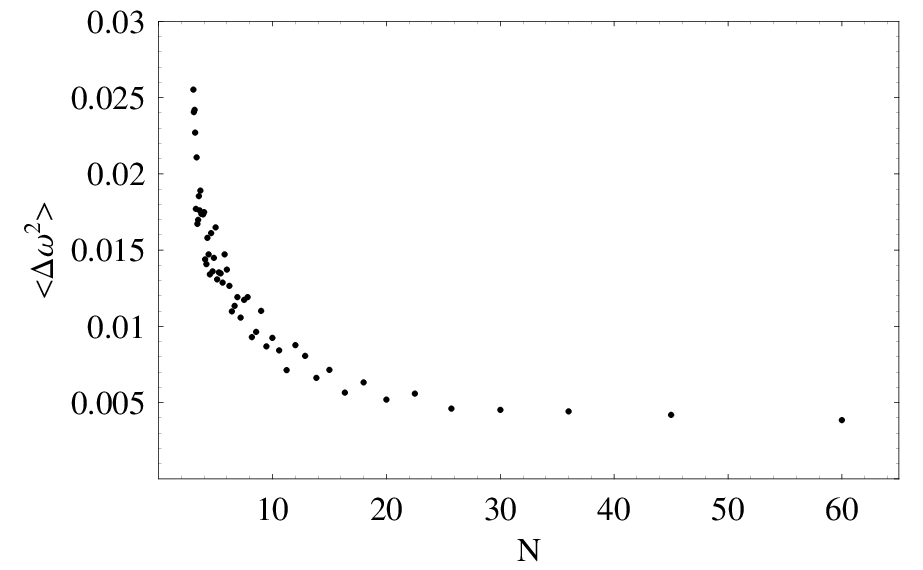
As already recalled, the relevant parameter for the geometrical cancellation usually related to holonomic gates in the adiabatic regime is the number of fluctuations of the noise during the gate operational time (denoted $N$ ). This effect is related only to the swept solid angle and is independent of the chosen operational time. If the number of cycles of the noise is large enough, the fluctuations in the solid angle spanned by the loop are expected to become negligible. To be more specific suppose that, after a noisy loop, the swept solid angle is $\omega$ and the mean square over the realizations of the noise is $\langle\Delta\omega^{2}\rangle$ . In Fig. 7 the mean square is plotted as a function of the number of cycles of the noise; since, in the adiabatic limit, the gate depends only on the swept solid angle, the fluctuations of the gate are expected to have the same behavior as the fluctuations in the solid angle.

As already explained in the previous section, Fig. 6 shows the average gate fidelity as a function of the adimensional typical noise frequency $(\Omega\tau_{\mathrm{step}})^{-1}$ for several values of the evolution time which correspond to the first four optimal operational times. The plot shows an analogous behavior of the fidelity as a function of the typical noise frequency independently of the particular value of the operational time; moreover, the minimum of the fidelity is reached in correspondence of $(\Omega\tau_{\mathrm{step}})^{-1}\simeq 0.5$ for all the values of the operational time considered. In order to cast some light on the nature of the cancellation effect, the same data are plotted in Fig. 8 as functions of the number of fluctuations of the noise (notice that $N=\Omega\tau(\Omega\tau_{\mathrm{step}})^{-1}$ ).

A direct comparison of figures 6 and 8 suggests that the relevant quantity which accounts for the mechanism of cancellation of the effects of the noise is its typical frequency $(\Omega\tau_{\mathrm{step}})^{-1}$ and not only the number of fluctuations $N$ . On the other hand, the fluctuations of the solid angle around the ideal value ( $\pi/2$ ) start to be negligible for $N>20$ ; a comparison with the curve for the fourth optimal working point (squares in Fig. 8) suggests that the recovery of the fidelity for long cyclic evolution times is given also by geometric cancellation.

For non adiabatic evolution times one can imagine the existence of a different mechanism which accounts for the observed cancellation of the noise effects for sufficiently fast noise which is related to a dynamical instead of geometrical cancellation. A dynamical effect could not be directly related to the swept solid angle: in this case the relevant parameter is expected to be the typical time of the noise $\tau_{\mathrm{step}}$ and a dynamical cancellation of the noise should appear if its typical frequency is sufficiently large compared to the system frequency, namely $(\Omega\tau_{\mathrm{step}})^{-1}\gg 1$ . Of course this condition implies, for fixed operational time $\tau$ , that $N\gg 1$ (the usual condition for geometric cancellation); nevertheless, as Fig. 6 shows, a cancellation of the noise effects appears on a frequency scale $(\Omega\tau_{\mathrm{step}})^{-1}\simeq 1$ independently of the chosen value of the operational time, thus suggesting a dynamical mechanism for the noise cancellation at least for the first four optimal operational times.

The fact that in the non adiabatic regime the robustness has a dynamical origin can also explain why the minimum value of the fidelity tends to decrease for increasing values of $\tau^{*}$ : if the geometric cancellation is not present, the noise is less effective in disturbing the system when the evolution time is short.

V Conclusions

In this paper we have considered the influence of parametric noise on the efficiency of a non adiabatic holonomic gate which is known to be robust in the ideal case. Three models of parametric noise have been discussed in the case of finite operational time. The average gate fidelities for all the models of noise considered here present an analogous qualitative behavior. For each of the three models the non ideal gate presents a breakdown of the average gate fidelity for small frequencies of the noise (compared to the system Bohr frequency), while a high value of the fidelity is reached for noise with higher frequencies. This can lead to say that the presence of a “resonant frequency” for the breakdown of $F$ is a general feature of any model of parametric noise.

We want to stress again that the usual argument in favor of the robustness of holonomic quantum computation is based on the purely geometric nature of the holonomy group that describes the adiabatic transformations. Since the dynamics has a completely geometric character only in the adiabatic limit, the robustness of adiabatic gates is, in this sense, just a consequence of the adiabatic theorem. Despite these considerations, our calculations show that, at least in certain situations, the first optimal operational time can be preferable to longer operational times with regards to the robustness of the corresponding gate against parametric noise.

Nevertheless, our results lead to the conclusion that the observed revivals of the fidelity for sufficiently fast noises is mainly due to dynamical instead of geometrical effects. Our conclusion is that, in the range of operational times considered here, the observed cancellation effects are mainly related to a dynamical average over fast oscillations of the noise $(\Omega\tau_{\mathrm{step}})^{-1}\gg 1$ and there is no relevant connection with the swept solid angle which plays a crucial role for the usual argument in favor of robustness of the holonomic computation in the adiabatic regime.

Acknowledgements.

This work is partly supported by the European Community through the Integrated Project EuroSQIP and by the bilateral Italian–Japanese Projects II04C1AF4E on “Quantum Information, Computation and Communication” of the Italian Ministry of Education, University and Research. G.F. thanks Paolo Facchi, Saverio Pascazio and Gianni Costantini for useful discussions and the Quantum Transport Group at TU Delft for kind hospitality and support.

References

(1) M. A. Nielsen, I. L. Chuang, Quantum Computation and Quantum Information (Cambridge University Press, Cambridge, 2000).
(2) G. Benenti, G. Casati and G. Strini, Principles of Quantum Computation and Information (World Scientific, Singapore, 2004).
(3) H. P. Breuer, F. Petruccione, The Theory of Open quantum Systems (Oxford University Press, Oxford, 2002).
(4) R. Alicki, M. Horodecki, P. Horodecki, R. Horodecki, L. Jacak and P. Machnikowski, 70, 010501(R) (2004); K. Roszak, A. Grodecka, P. Machnikowski and T. Kuhn, Phys. Rev. B 71, 195333 (2005).
(5) D. J. Wineland, C. Monroe, W. M. Itano, D. Leibfried, B. E. King, D. M. Meekhof, J. Res. Natl. Inst. Stand. Technol. 103, 259 (1998).
(6) P. Zanardi, M. Rasetti, Phys. Lett. A 264, 94 (1999).
(7) J. Pachos, P. Zanardi and M. Rasetti, Phys. Rev. A 61, 010305(R) (1999).
(8) M. Nakahara, Geometry, topology and physics, 2nd Ed., (IoP publishing, Bristol, 2005).
(9) K. B. Marathe, G. Martucci, The Mathematical Foundations of Gauge Theories (North-Holland, Amsterdam, 1992).
(10) M. V. Berry, Proc. R. Soc. Lond. A 392, 45 (1984); B. Simon, Phys. Rev. Lett. 51, 2167 (1983).
(11) F. Wilczek and A. Zee, Phys. Rev. Lett. 52, 2111 (1984).
(12) J. Pachos, P. Zanardi, Int. J. Mod. Phys. B 15, 1257 (2001).
(13) T. Kato, J. Phys. Soc. Jap. 5, 435 (1951).
(14) Y. Aharonov, J. Anandan, Phys. Rev. Lett. 58, 1593 (1987).
(15) J. Anandan, Phys. Lett. A 133, 171 (1988).
(16) G. De Chiara, G. M. Palma, Phys. Rev. Lett. 91, 090404 (2003).
(17) P. Solinas, P. Zanardi and N. Zanghì, Phys. Rev. A 70, 042316 (2004).
(18) S.-L. Zhu and P. Zanardi, Phys. Rev. A 72, 020301(R) (2005).
(19) A. Carollo, I. Fuentes-Guridi, M. França Santos and V. Vedral, Phys. Rev. Lett. 90, 160402 (2003).
(20) A. Carollo, I. Fuentes-Guridi, M. França Santos and V. Vedral, Phys. Rev. Lett. 92, 020402 (2004).
(21) I. Fuentes-Guridi, F. Girelli, E. Livine, Phys. Rev. Lett. 94, 020503 (2005).
(22) D. Parodi, M. Sassetti, P. Solinas, P. Zanardi, N. Zanghì, Phys. Rev. A 73, 052304 (2006).
(23) L.-A. Wu, P. Zanardi, D. A. Lidar, Phys. Rev. Lett. 95, 130501 (2005).
(24) G. Florio, P. Facchi, R. Fazio, V. Giovannetti and S. Pascazio, Phys. Rev. A 73, 022327 (2006).
(25) A. Trullo, P. Facchi, R. Fazio, G. Florio, V. Giovannetti, S. Pascazio, Las. Phys. 16, 1478 (2006).
(26) G. Florio, Open Sys. & Information Dyn. 13, 263 (2006).
(27) L.-M. Duan, J. I. Cirac, P. Zoller, Science 292, 1695 (2001).
(28) G. Falci, R. Fazio, G. M. Palma, J. Siewert and V. Vedral, Nature 407, 355 (2000).
(29) L. Faoro, J. Siewert and R. Fazio, Phys. Rev. Lett. 90, 028301 (2003).
(30) P. Solinas, P. Zanardi, N. Zanghì and F. Rossi, Phys. Rev. A 67, 062315 (2003).
(31) M. S. Sarandy, D. A. Lidar, Phys. Rev. Lett. 95, 250503 (2005).
(32) M. S. Sarandy, D. A. Lidar, Phys. Rev. A 71, 012331 (2005); 73, 062101 (2006).
(33) M. Born and V. Fock, Z. Phys. 51, 165 (1928).
(34) M. A. Nielsen, Phys. Lett. A 303, 249 (2002); M. D. Bowdrey, D. K. L. Oi, A. J. Short, K. Banaszek and J. A. Jones, ibid. 294, 258 (2002); M. Horodecki, P. Horodecki and R. Horodecki, Phys. Rev. A 60, 1888 (1999).