This document contains

the doctoral dissertation (94 pages)

submitted to

the Graduate School

of the University of Tokyo

and

the slides (mainly Japanese, 14 pages herein,

originally a PowerPoint file with 28 slides)

used at the presentation

for the degree of the doctor

in Octover 1995.

Dr. of Information Science and Technology,

Toshiyuki Shimono

“Beam me over,” Alice: A cricket’s quantum journey

This thesis addresses two known quantities in quantum information science: (1) entanglement cost, and (2) Holevo capacity. These quantities will be crucial values when teleportation becomes common in daily life, perhaps centuries from now.

Assume that Alice desires to send a singing Japanese cricket to her friend Bob in America, and that Alice and Bob already share a quantum entanglement. First, Alice sends Bob a mass of information bits resulting from the interaction between the cricket she holds in her hand and half of the entanglement. Subsequently, Bob receives the information bits and manipulates the other half of the entanglement, transforming them back into the original cricket. Examining this situation from an instrumental engineering viewpoint, quantifying the amount of the quantum entanglement and the number of information bits is crucial for this transmission. If both values are enough, Alice could even send herself to Bob’s place instead of the tiny cricket.

The topics of this thesis therefore are: (1) the mathematical properties of the entanglement cost, such as whether it is an additive measure similar to normal length or weight; and (2) how to calculate the Holevo capacity, an ultimately achievable limit of the information conveyance capacity of an information channel, such as of a single photon passing through an optical fiber or space. These two distinct quantities are magically tied together by several “additive or not” hypotheses, which await mathematical proof.

$>>$ The submitted thesis is from the next page. $>>$

{acknowledge}

I would like to say thank you to all the following people: Prof. Hiroshi Imai, my supervisor; Prof. Keiji Matsumoto, the former head of the Tokyo branch of the Imai project; Prof. Masahito Hayashi, the present head. Jozef Gruska, the advisor of the project; Hwang Won Young, Wang Xian Bing, and Masahiro Hachimori, with whom I talked over many issues; Andreas Winter, Fan Heng, and Mary Beth Ruskai, the coauthors of our articles, who offered me many experiences; Jumpei Niwa; Takako Sakuragi; Takashi Yamada; Jun Hasegawa; François Le Gall; Sonoko Moriyama, and Mayumi Oto. I do not have enough time nor memory to recall all those who have supported me — thus please forgive me for any gross omission.

I have conducted research in my way to hopefully be the root of a new methodology in the realm of research, rather than imitating others. Nonetheless I will not forget that this dissertation could not have been completed without a lot of support from those mentioned above. Their help was immense, and I hope to continue to utilize it beyond this work.

Toshiyuki Shimono, December 2004.

Part I Prologue – Introduction and Background –

Chapter 1 Quantum Information Science

Quantum information science, the consolidation of the rules and the intelligence of this physical world, is the emerging essence of science. We need tools to understand and investigate this developing science.

Prior to the chapter of the introduction, we present here what the quantum information science is in this chapter. Concepts used in this dissertation are explained, compactly, neatly, and hopefully coherently.

1 What is a quantum state?

What is a quantum state? It specifies a specific physical state at a given time in the framework of quantum physics. Quantum physics attempts to explain most everything in the world, especially the micro-world. Generally, a quantum state is the ‘‘superposition’’ of multiple specified states, as often depicted by Schrödinger’s cat, that is the superposition of a living cat and a dead cat. One needs to understand such peculiar phenomena because information devices are becoming smaller and smaller toward nanometer world. Predictions say that fifteen or twenty years from now, each bit of information will be contained in as few as one atom as technology continues to grow exponentially, as it has for more than forty years.

In this dissertation, we deal solely with static quantum states; we do not consider physical continuous time transition on states that might involve the Schrödinger equation, that is, $H(t){|{\psi(t)}\rangle}=\sqrt{-1}\hbar\frac{\partial}{\partial t}{|{\psi(t)}\rangle}$ . Still, in the static framework, there are many interesting phenomena such as quantum entanglement. It is an anomalous correlation on two sites or more, which is not depicted in the framework of classical views of physics. Einstein et al. opposed quantum physics because quantum entanglement seemed to raise the issue of superluminal communication [Einstein-Podolsky-Rosen 35]. Quantum entanglement is, however, being experimentally confirmed, and many protocols utilizing it are proposed and being tested experimentally.

Here, again, we ask “What is a quantum state?” The definitions, mainly from mathematical viewpoints, follows.

1.1 Pure state and its tensor product

1.1.1 Pure states

A pure state $\left|\psi\right\rangle$ is a vector of which the length is one, dwelling on a specified vector space, or a Hilbert space, of a complex number field. One can represent it by a column vector of which the elements are complex numbers as,

\left|\psi\right\rangle=\left(\begin{array}[]{c}x_{1}\\ x_{2}\\ \vdots\\ x_{d}\end{array}\right)

with the conditions $x_{1},x_{2},\ldots,x_{d}\in\mathbb{C}$ and $|x_{1}|^{2}+|x_{2}|^{2}+\ldots+|x_{d}|^{2}=1$ . Note that this is just a representation, and a vector treated in quantum information science is an element of a vector space, more precisely a Hilbert space over complex number field. The space is spanned by some bases, such as $\{{|{\leftrightarrow}\rangle},{|{\updownarrow}\rangle}\}$ , $\{{|{\uparrow}\rangle},{|{\downarrow}\rangle}\}$ , or simply $\{{|{1}\rangle},{|{2}\rangle},\ldots,{|{d}\rangle}\}$ , as exemplified in the next.

The polarization of a single photon:

Figure 1: This figure depicts how to prepare photons with the polarization with

\cos\theta\,{|{\leftrightarrow}\rangle}+\sin\theta\,{|{\updownarrow}\rangle}

The polarization of a photon flying in $z$ -direction is conceptually represented in a two-dimensional space with bases ${|{\leftrightarrow}\rangle}$ and ${|{\updownarrow}\rangle}$ , that represent $x$ -directional and $y$ -directional polarization, respectively. If the polarization angle is $\theta$ on the $xy$ -plane, the state of the photon is represented as ${|{\theta}\rangle}=\cos\theta\,{|{\leftrightarrow}\rangle}+\sin\theta\,{|{\updownarrow}\rangle}$ that is the superposition of ${|{\leftrightarrow}\rangle}$ and ${|{\updownarrow}\rangle}$ with coefficients $\cos\theta$ and $\sin\theta$ . This vector ${|{\theta}\rangle}$ is represented as $\left(\begin{smallmatrix}\cos\theta\\ \sin\theta\end{smallmatrix}\right)$ . See Fig.1. Note that the coefficients can be any complex number as long as their squared summation is one. $\cos\theta\,{|{\leftrightarrow}\rangle}+e^{\sqrt{-1}\gamma}\sin\theta\,{|{\updownarrow}\rangle}$ is such an example, which can be considered to have the phase shift of $\gamma$ in the factor of $\updownarrow$ , and it is called to have circular or elliptical polarization.

As a physical aspect, the dimensionality of two is enough for the vector space of the polarization of a photon. In principle, the most possible measurement of the polarization of each single photon is equivalent to check whether the photon passes through a prepared polarizing plate, and the passed photon loses the information of the polarization. Thus all the information the observer can get about the polarization of the photon is as few as two possibilities, which is related to the dimensionality of two here.

The magnetic moment of a single silver atom:

Figure 2: Stern-Gerlach experiment

Each silver atom has its momentum state on the vector space spanned by ${|{\uparrow}\rangle}$ and ${|{\downarrow}\rangle}$ . The state is written as $\alpha{|{\uparrow}\rangle}+\beta{|{\downarrow}\rangle}$ that is a superposition of ${|{\uparrow}\rangle}$ and ${|{\downarrow}\rangle}$ . Physically, the momentum can be measured by making the atom flying through nonuniform magnetic field, and the atoms curve in two possible directions. The measurement is done by observing which of the two directions the atom has curved. If the magnetic field is set up to detect whether the atom has the moment of ${|{\uparrow}\rangle}$ or of ${|{\downarrow}\rangle}$ , then the atom turns to become ${|{\uparrow}\rangle}$ or ${|{\downarrow}\rangle}$ by curving into the corresponding directions with the possibility $|\alpha|^{2}$ or $|\beta|^{2}$ , respectively. This experiment is called Stern-Gerlach experiment , which is a typical experiment to show the physical phenomenon of quantization of the magnetic moment of atoms.

A physical system is called a $d$ -level system when the system is a space for $d$ -dimensional vectors.

The physical system to be observed the polarization of a single photon or the magnetic momentum of a single silver atom is a typical $2$ -level system.

1.1.2 Ket and bra

As a mathematical convenience, ${|{\psi}\rangle}$ is called a ket vector. ${\langle{\psi}|}$ is the Hermitian transpose, or the conjugate transpose of ${|{\psi}\rangle}$ , which is called a bra vector. The former is considered a column vector, and the latter is considered a row vector on matrix arithmetic. Thus, one can consider ${|{\psi}\rangle}\!{\langle{\psi}|}$ to be a square matrix.

1.1.3 Tensor product of pure states

You might like to consider the state of a system which contains two particles and more. Here, we give the concepts of tensor product for two pure states. The tensor product $\mathcal{H}\otimes\mathcal{H}^{\prime}$ of two spaces $\mathcal{H}$ and $\mathcal{H}^{\prime}$ is the $d\times d^{\prime}$ -dimensional vector space when $\mathcal{H}$ and $\mathcal{H}^{\prime}$ are $d$ - and $d^{\prime}$ - dimensional, respectively. The tensor product of two vectors of $\mathcal{H}$ and $\mathcal{H}^{\prime}$ is defined as follows:

\left(\begin{array}[]{c}x_{1}\\ x_{2}\\ \vdots\\ x_{d}\\ \end{array}\right)\otimes\left(\begin{array}[]{c}y_{1}\\ y_{2}\\ \vdots\\ y_{d^{\prime}}\\ \end{array}\right)=\left(\begin{array}[]{c}x_{1}y_{1}\\ x_{1}y_{2}\\ \vdots\\ x_{1}y_{d^{\prime}}\\ x_{2}y_{1}\\ \vdots\\ x_{2}y_{d^{\prime}}\\ \vdots\\ \vdots\\ x_{d}y_{d^{\prime}}\\ \end{array}\right).

(1)

For example, $\left(\begin{smallmatrix}\sqrt{0.3}\\ \sqrt{0.7}\end{smallmatrix}\right)\otimes\left(\begin{smallmatrix}\sqrt{0.4}\\ \sqrt{0.6}\end{smallmatrix}\right)=\left(\begin{smallmatrix}\sqrt{0.12}\\ \sqrt{0.18}\\ \sqrt{0.28}\\ \sqrt{0.42}\end{smallmatrix}\right)$ . By convention, ${|{\phi_{1}}\rangle}\otimes{|{\phi_{2}}\rangle}$ is sometimes abbreviated as ${|{\phi_{1}}\rangle}{|{\phi_{2}}\rangle}$ or ${|{\phi_{1}\,\phi_{2}}\rangle}$ . One can consider that tensor product of states of two particles is considered to be the state of the whole two particles.

1.2 Mixed states and tensor product

A mixed state is represented by a semi-positive Hermitian matrix¹¹ 1 Semi-positive Hermitian matrix: A matrix $\rho$ is Hermitian as long as it satisfies $\rho=\rho^{\dagger}$ . In this case, all its eigenvalues are real numbers. It is semi-positive when all its eigenvalues are equal to or larger than zero. of which the trace, or the summation of the diagonal elements, is $1$ . It is regarded as a stochastic mixture of multiple pure states $\{{|{\psi_{i}}\rangle}\}_{i}$ , as $\rho=\sum_{i}p_{i}{|{\psi_{i}}\rangle}\!{\langle{\psi_{i}}|}$ with $\{p_{i}\}_{i}$ a probability distribution. Note that stochastic mixture is a different notion from superposition of pure states. The semi-positive Hermitian matrix of a mixed state is called the density matrix. This dissertation employs the conventional phrase “a state $\rho$ on $\mathcal{H}$ ” or “a state $\rho$ on $\mathbb{C}^{d}$ ” if $\rho$ is a $d\times d$ semi-positive matrix of which the trace is one. Notation $\mathcal{B}(\mathcal{H})$ is employed to explicitly specify the set of states on a Hilbert space $\mathcal{H}$ .

Notation 1.1 (mixed states)

$\mathcal{B}(\mathcal{H})$ is the set of any mixed states $\rho$ on a Hilbert space $\mathcal{H}$ . When $\mathcal{H}$ is $d$ -dimensional, $\mathcal{B}(\mathcal{H})$ is equal to the set of $d\times d$ semi-positive matrix of which the trace is one.

Note that a pure state ${|{\phi}\rangle}$ is regarded to be equal to a mixed state ${|{\phi}\rangle}\!{\langle{\phi}|}$ as a stochastic mixture of a single state ${|{\phi}\rangle}$ with 100% weight. Mixed states other than pure states may be called non-pure states.

The tensor product of mixed states is an expansion to the tensor product of pure states, as follows:

\begin{split}&\left(\begin{array}[]{ccc}a_{11}&\cdots&a_{1d}\\ \vdots&&\vdots\\ a_{d1}&\dots&a_{dd}\end{array}\right)\otimes\left(\begin{array}[]{ccc}b_{11}&\cdots&b_{1d^{\prime}}\\ \vdots&&\vdots\\ b_{d^{\prime}1}&\dots&b_{d^{\prime}d^{\prime}}\end{array}\right)\hfill\\ &\qquad\hfill=\left(\begin{array}[]{ccc}\begin{array}[]{ccc}a_{11}b_{11}&\cdots&a_{11}b_{1d^{\prime}}\\ \vdots&&\vdots\\ a_{11}b_{d^{\prime}1}&\dots&a_{11}b_{d^{\prime}d^{\prime}}\end{array}&\cdots&\begin{array}[]{ccc}a_{1d}b_{11}&\cdots&a_{1d}b_{1d^{\prime}}\\ \vdots&&\vdots\\ a_{1d}b_{d^{\prime}1}&\dots&a_{1d}b_{d^{\prime}d^{\prime}}\end{array}\\ \vdots&&\vdots\\ \begin{array}[]{ccc}a_{d1}b_{11}&\cdots&a_{d1}b_{1d^{\prime}}\\ \vdots&&\vdots\\ a_{d1}b_{d^{\prime}1}&\dots&a_{d1}b_{d^{\prime}d^{\prime}}\end{array}&\dots&\begin{array}[]{ccc}a_{dd}b_{11}&\cdots&a_{dd}b_{1d^{\prime}}\\ \vdots&&\vdots\\ a_{dd}b_{d^{\prime}1}&\dots&a_{dd}b_{d^{\prime}d^{\prime}}\end{array}\end{array}\right).\end{split}

(2)

1.3 Arithmetic on states

This subsection deals with some arithmetic on quantum states, such as, tracing out, von Neumann entropy and quantum divergence.

Notation 1.2 (trace out, tracing out)

For a state $\rho=\sum_{i}p_{i}\,\rho_{i}^{A}\otimes\rho_{i}^{B}$ on $\mathcal{H}_{A}\otimes\mathcal{H}_{B}$ , tracing out operations are defined as follows. Tracing out the space of $\mathcal{H}_{B}$ from $\rho$ is defined as

\mathop{\mathrm{Tr}}\nolimits_{B}\rho=\sum_{i}p_{i}\,(\mathop{\mathrm{Tr}}\nolimits\rho_{i}^{B})\cdot\rho_{i}^{A},

(3)

resultingly a state on $\mathcal{H}_{A}$ . Similarly, tracing out the space of $\mathcal{H}_{A}$ is,

\mathop{\mathrm{Tr}}\nolimits_{A}\rho=\sum_{i}p_{i}\,(\mathop{\mathrm{Tr}}\nolimits\rho_{i}^{A})\cdot\rho_{i}^{B}\text{\quad on \quad}\mathcal{H}_{B}.

(4)

$\mathop{\mathrm{Tr}}\nolimits_{B}$ is an operation tracing out the space of $B$ , leaving the space of $A$ . Conversely, $\mathop{\mathrm{Tr}}\nolimits_{A}$ is an operation tracing out the space of $A$ , leaving the space of $B$ . Concrete examples of tracing out appear at pp.25.

Notation 1.3 ( $\log\rho,\sqrt{\rho}$ )

For a semi-positive Hermite matrix $\rho$ , $\log\rho$ and $\sqrt{\rho}$ are defined as follows:

\begin{split}&\log\rho=U\,{\rm diag}\,[\log t_{1},\dots,\log t_{d}]\,U^{\dagger}\\ &\qquad\qquad\qquad\text{ for }\rho=U\,{\rm diag}\,[t_{1},\dots,t_{d}]\,U^{\dagger},\end{split}

(5)

and

\begin{split}&\sqrt{\rho}=U\,{\rm diag}\,[\sqrt{t_{1}},\dots,\sqrt{t_{d}}]\,U^{\dagger}\\ &\qquad\qquad\qquad\text{ for }\rho=U\,{\rm diag}\,[t_{1},\dots,t_{d}]\,U^{\dagger},\end{split}

(6)

where ${\rm diag}\,[t_{1},\dots,t_{d}]$ is the diagonal matrix $\left(\begin{smallmatrix}t_{1}&&\\ &\ddots&\\ &&t_{d}\end{smallmatrix}\right)$ , and $U$ is a unitary matrix.

To keep consistency and to avoid confusion the following conventions are employed here:

\log 0

is treated as

-\infty

, additionally,

0\log 0

is treated as

0

(7)

Notation 1.4 (von Neumann entropy, [Neumann 32])

S(\rho)=-\mathop{\mathrm{Tr}}\nolimits\rho\log\rho

(8)

One can show that $S(\rho)$ is equal to the Shannon entropy of the whole eigenvalues of $\rho$ , that is, $S(\rho)=\sum(-\lambda_{i}\log\lambda_{i})$ with $\{\lambda_{i}\}$ being the eigenvalues of $\rho$ . Note that for pure states ${|{\phi}\rangle}\!{\langle{\phi}|}$ , the von Neumann entropy is zero.

Notation 1.5 (quantum divergence)

The quantum divergence for two mixed states from the same space are defined as follows:

H(\rho||\sigma)=\mathop{\mathrm{Tr}}\nolimits(\rho\log\rho-\rho\log\sigma).

(9)

Quantum divergence is also called quantum relative entropy. Quantum divergence has following properties, as it is similar to a measure of distance of two states, but it lacks the property of symmetry.

Proposition 1.6 (basic properties of $H(\cdot||\cdot)$ )

	$\displaystyle H(\rho\|\|\sigma)\geq 0,$		(10)
	$\displaystyle H(\rho\|\|\sigma)=0\quad\Leftrightarrow\quad\rho=\sigma,$		(11)
	$\displaystyle H(\cdot_{1}\|\|\cdot_{2})\not\equiv H(\cdot_{2}\|\|\cdot_{1}).$		(12)

1.4 Mapping on quantum states

This subsection deals with mapping on quantum states. In this dissertation, a ‘‘map’’ or ‘‘mapping’’ means a linear map. One can associate a mapping as a time transition of a quantum state, formalized as a quantum channel later.

Notation 1.7 (tensor product of mapping)

For two mappings $\Lambda_{1}$ and $\Lambda_{2}$ , the tensor product $\Lambda_{1}\otimes\Lambda_{2}$ is defined based on a restriction that $\Lambda_{1}\otimes\Lambda_{2}(\rho_{1}\otimes\rho_{2})=\Lambda_{1}(\rho_{1})\otimes\Lambda_{2}(\rho_{2})$ for any input $\rho_{1}$ of $\Lambda_{1}$ and any input $\rho_{2}$ of $\Lambda_{2}$ .

Notation 1.8 (complete positivity, CP-ness)

A complete positive map $\Lambda$ is a map such that for any (finite) dimensional identity map $I$ , $\Lambda\otimes I$ maps a semi-positive Hermitian matrix into a semi-positive Hermitian matrix. This complete positivity is also called CP-ness.

Notation 1.9 (trace preserving, TP-ness)

A trace preserving map $\Lambda$ is a map satisfying $\mathop{\mathrm{Tr}}\nolimits\Lambda\rho=\mathop{\mathrm{Tr}}\nolimits\rho$ for any $\rho$ . This trace preserving property is also called TP-ness.

Notation 1.10 (CPTP-ness)

Combining the two terms above, a map of CP and TP is a CPTP map.

Notation 1.11 (Bures distance and the fidelity)

The fidelity between given two states is defined as

F(\rho,\sigma)=\mathop{\mathrm{Tr}}\nolimits\sqrt{\,\sqrt{\rho}\,\sigma\,\sqrt{\rho}\,}.

(13)

The Bures distance is defined as

B(\rho,\sigma)=2\sqrt{1-F(\rho,\sigma)}.

(14)

Proposition 1.12

The fidelity has the properties such as:

$\displaystyle F(\cdot_{1},\cdot_{2})$	$\displaystyle\leq$	$\displaystyle 1$	(15)
$\displaystyle F(\cdot_{1},\cdot_{1})$	$\displaystyle\equiv$	$\displaystyle 1$	(16)
$\displaystyle F(\cdot_{1},\cdot_{2})$	$\displaystyle\equiv$	$\displaystyle F(\cdot_{2},\cdot_{1})$	(17)
$\displaystyle F({\|{\psi}\rangle}\!{\langle{\psi}\|},{\|{\phi}\rangle}\!{\langle{\phi}\|})$	$\displaystyle=$	$\displaystyle\langle\psi\|\phi\rangle\quad\text{ for the same dimensional }{\|{\psi}\rangle},{\|{\phi}\rangle}.$	(18)

The fidelity is considered to be how truly a quantum state is transmitted. $100\%$ fidelity, or the fidelity being one is the perfect transmission, which means the transmission is done without losing information the quantum states held. Note that in (18), the left hand side is determined even if the dimension of ${|{\psi}\rangle}$ and ${|{\phi}\rangle}$ is different while the right hand side is not defined.

The Bures distance (14) is a derivation from the fidelity to take on the properties of a distance. The nearer upward to 1 or 100% the fidelity between two states become, the smaller downward to 0 the distance between the two states become.

2 A quantum channel and its capacity

There are various frameworks to deal with time transition of a quantum states as follows:
(1) Schrödinger equation — $H{|{\psi}\rangle}=\sqrt{-1}\hbar\frac{\partial}{\partial t}{|{\psi}\rangle}$
(2) Quantum circuit — and,
(3) Quantum channel — .

(1) and (2) treat only pure states, and (3) treats mixed states generally. To investigate quantum information science, treating mixed states is necessary.

Definition 1.13 (quantum channel)

A quantum channel $\Lambda$ is a CPTP map (see Notation 1.10). Thus, $(\Lambda\rho)\otimes\sigma$ is a quantum state for any quantum state $\sigma$ . (See Fig.3.)

Figure 3: A quantum channel must be a CPTP map in order to keep the whole world a quantum state that is represented as a semi-positive Hermitian matrix.

Because of the linearity of mappings of quantum channel, $\rho^{\prime}=\Lambda(\rho)$ is abbreviated as $\rho^{\prime}=\Lambda\rho$ .

Definition 1.14 (Tensor product of channels)

For channels $\Lambda$ and $\Lambda^{\prime}$ , the tensor product of these channels $\Lambda\otimes\Lambda^{\prime}$ is a linear map which maps $\rho\otimes\rho^{\prime}$ to $(\Lambda\rho)\otimes(\Lambda^{\prime}\rho^{\prime})$ where $\rho$ is any input of $\Lambda$ and $\rho^{\prime}$ is any input of $\Lambda^{\prime}$ .

The concept of tensor product is natural to consider multiple channels in the physical world.

Theorem 1.15 (Stinespring’s dilation)

For any quantum channel $\Lambda:\rho\mapsto\rho^{\prime}$ , there exists some auxiliary space $K$ , some auxiliary state $\sigma$ , and a unitary matrix $U$ such that

\rho^{\prime}=\mathop{\mathrm{Tr}}\nolimits_{K}U\left(\rho\otimes\sigma\right)U^{\dagger}.

(19)

Now we have formalized what a quantum channel is. Then, how is the capacity of the channel considered, i.e., how much information can be carried from the sender to the receiver in a remote place through a quantum channel? One of the formalizations is the Holevo capacity. The definition follows.

Definition 1.16 (Holevo capacity, [Holevo 73, Holevo 98, Schumacher-Westmoreland 97])

The Holevo capacity $C$ of a given quantum channel $\Lambda$ is as follows:

C(\Lambda)=\max_{n;\rho_{1},\dots,\rho_{n};p_{1},\dots,p_{n}}S(\sum_{i=1}^{n}p_{i}\,\Lambda\rho_{i})-\sum_{i=1}^{n}p_{i}\,S(\Lambda\rho_{i}),

(20)

where $n\in\mathbb{N},p_{i}>0,\sum_{i=1}^{n}p_{i}=1$ and every $\rho_{i}$ s is an input of the channel $\Lambda$ .

The optimized $n$ in (20) is regarded as the number of kinds of the input states of the channel $\Lambda$ , when the communication capacity attains the Holevo capacity of $\Lambda$ in an asymptotic sense.

Theorem 1.17 ([Ohya-Petz-Watanabe 97])

C(\Lambda)=\min_{\sigma}\max_{\rho}H(\Lambda\rho\,||\,\Lambda\sigma)

(21)

where $\sigma$ and $\rho$ are the inputs of the channel $\Lambda$ .

Physically, the Holevo capacity is a classical information capacity of a given quantum channel at which input particles are not allowed to be entangled with each other, and the output particles are measured collectively. To fully utilize quantum aspects of a quantum channel, one might consider the capacity at which the input particles are freely entangled with each other to send a message. This capacity is called the full capacity.

Definition 1.18 (Full capacity)

\bar{C}(\Lambda)=\lim_{n\to\infty}C(\Lambda^{\otimes n})/n

(22)

3 Entanglement and its quantification

This section defines the quantum entanglement in the case of a bipartite system.

When considering bipartite quantum entanglement, we often think of two figures, named Alice and Bob. Their spaces, at which quantum states are considered, are represented as Hilbert spaces $\mathcal{H}_{A}$ and $\mathcal{H}_{B}$ , respectively.

Definition 1.19 (entanglement)

For a pure state ${|{\phi}\rangle}\in\mathcal{H}_{A}\otimes\mathcal{H}_{B}$ , ${|{\phi}\rangle}$ is said to be entangled
if ${|{\phi}\rangle}$ cannot be represented in a form ${|{\phi_{A}}\rangle}\otimes{|{\phi_{B}}\rangle}$ with ${|{\phi_{A}}\rangle}\in\mathcal{H}_{A}$ and ${|{\phi_{B}}\rangle}\in\mathcal{H}_{B}$ .
For a mixed state $\rho$ on $\mathcal{H}_{A}\otimes\mathcal{H}_{B}$ , $\rho$ is said to be entangled
if $\rho$ cannot be represented as $\sum_{i}p_{i}{|{\phi_{i}}\rangle}\!{\langle{\phi_{i}}|}$
with unentangled pure states ${|{\phi_{i}}\rangle}$ and a probability distribution $\{p_{i}\}$ .

An unentangled state is called separable. To explicitly refer to two system which are entangled, notation $\mathcal{H}_{A}:\mathcal{H}_{B}$ is used in this dissertation. When considering the entanglement, our interest reside at two sites (Alice and Bob) rather than their space $\mathcal{H}_{A}$ and $\mathcal{H}_{B}$ . In such a case we just denote Alice:Bob or A:B.

Definition 1.20 (LOCC, cf. [Bennet-DiVicenzo-Smolin-Wootters 96])

LOCC operations (standing for Local Operation plus Classical Communication) for a bipartite system are defined to be comprised only of:
(1) local CPTP operations on each side, and
(2) communications between the two sites by only classical means.
Classical communication means the following: One side physically measures the state of its own system, and transmit the output of the measurement to the other side. Based on this information, the receiver may perform physical operations of its own system. Physical measurements are formalized to be the concept of POVM, which we do not take up in this dissertation.

Refer to caption — Figure 4: LOCC operations: Only Local Operations and Classical Communications are allowed. Joint operations or sending quantum information is prohibited if it is beyond the allowed operations.

There is a well-established entanglement measure for bipartite pure states.

Notation 1.21 (reduced von Neumann entropy)

The reduced von Neumann entropy for a bipartite state is defined as

\hskip 113.81102ptE^{\>\sf A:B}({|{\phi}\rangle})=S(\mathop{\mathrm{Tr}}\nolimits_{B}{|{\phi}\rangle}\!{\langle{\phi}|})\\ \qquad\qquad\qquad\mbox{ for a pure state }{|{\phi}\rangle}\in\mathcal{H}_{A}\otimes\mathcal{H}_{B}.\hskip 113.81102pt

(23)

One can easily confirm that $S(\mathop{\mathrm{Tr}}\nolimits_{B}{|{\phi}\rangle}\!{\langle{\phi}|})=S(\mathop{\mathrm{Tr}}\nolimits_{A}{|{\phi}\rangle}\!{\langle{\phi}|})$ thus $E^{\>\sf A:B}({|{\phi}\rangle}\!{\langle{\phi}|})=S(\mathop{\mathrm{Tr}}\nolimits_{A}{|{\phi}\rangle}\!{\langle{\phi}|})$ .

If a pure state is entangled, the reduced von Neumann entropy is larger than 0.

Example 1.22 (Bell state, Bell pair)

{|{\Phi^{\pm}}\rangle}=\frac{{|{00}\rangle}\pm{|{11}\rangle}}{\sqrt{2}},{|{\Psi^{\pm}}\rangle}=\frac{{|{01}\rangle}\pm{|{10}\rangle}}{\sqrt{2}}

(24)

are called the Bell states. These states ${|{\Phi^{+}}\rangle},{|{\Phi^{-}}\rangle},{|{\Psi^{+}}\rangle}$ and ${|{\Psi^{-}}\rangle}$ are often considered to be implicitly shared by Alice and Bob throughout this dissertation. Their reduced von Neumann entropy is 1.

Bell states are often considered to be units of quantum entanglement.

For bipartite mixed states, there are various candidates to measure quantum entanglement as follows.

Definition 1.23 (entanglement cost, entanglement distillation [Bennet-DiVicenzo-Smolin-Wootters 96])

The entanglement cost is defined as

E_{C}^{\>\sf A:B}(\rho)=\inf\left\{\>e\>\big|\>^{\forall}(\epsilon,\delta),^{\exists}(m,n,L):|e-\frac{m}{n}|\leq\delta,B\left(L({|{\Psi^{-}}\rangle}\!{\langle{\Psi^{-}}|}^{\otimes m}),\rho^{\otimes n}\right)\leq\epsilon\>\right\},

(25)

and the entanglement distillation is defined as

E_{D}^{\>\sf A:B}(\rho)=\sup\left\{\>e\>\big|\>^{\forall}(\epsilon,\delta),^{\exists}(m,n,L):|e-\frac{m}{n}|\leq\delta,B\left({|{\Psi^{-}}\rangle}\!{\langle{\Psi^{-}}|}^{\otimes m},L(\rho^{\otimes n})\right)\leq\epsilon\>\right\},

(26)

where $e\geq 0,\;\epsilon,\delta>0,\;m,n\in\mathbb{N}$ and $L(\cdot)$ is a LOCC operation. $B(\cdot,\cdot)$ is the Bures distance defined in (14).

The entanglement distillation $E_{D}$ is the asymptotic quantity of Bell states distilled from $\rho$ with LOCC operations. Thus, one can consider $E_{D}$ as a measure to quantify the entanglement as a resource to be used for quantum teleportation or quantum super dense coding.

The entanglement cost $E_{C}$ is the asymptotic quantity of Bell states necessary to produce $\rho$ with LOCC operations.

Definition 1.24 (entanglement of formation [Bennet-DiVicenzo-Smolin-Wootters 96])

The entanglement of formation is defined as

E_{F}^{\>\sf A:B}(\rho)=\min_{n;\,{|{\phi_{1}}\rangle},\ldots,{|{\phi_{n}}\rangle};\,p_{1},\ldots,p_{n}}\sum_{i=1}^{n}p_{i}E^{\>\sf A:B}({|{\phi_{i}}\rangle}\!{\langle{\phi_{i}}|}),

(27)

with $p_{i}>0,\sum_{i=1}^{n}p_{i}=1,\sum_{i=1}^{n}p_{i}{|{\phi_{i}}\rangle}\!{\langle{\phi_{i}}|}=\rho$ .

We may use the denotations $E(\cdot),E_{C}(\cdot),E_{D}(\cdot),E_{F}(\cdot)$ which omit the superscription $\sf A:B$ when the two sites are clear to consider entanglement.

Proposition 1.25 ( [Hayden-Horodecki-Terhal 01])

The following holds:

E_{C}(\rho)=\lim_{n\to\infty}\frac{E_{F}(\rho^{\otimes n})}{n}

(28)

This equality (28) is significant in that the conceptually defined $E_{C}$ represented as (25) has become mathematically defined by substituting (27) into (28). The calculation is, however, not simple, which leads to the main subject of this dissertation because (28) being substituted with (27) is in a limitation form over infinitely many optimization forms $\{E_{F}(\rho^{\otimes n})/n\}_{n=1}^{\infty}$ .

4 Example: a two-level system

This section presents properties of the Bloch sphere representing states on a qubit, or a 2-level system.²² 2 “Qubit” can be considered as a unit of quantum information as the counterpart of the concept of “bit” of the current information theory. Qubit is named by Benjamin Schumacher.

4.1 Bloch sphere and the Stokes parameterization

Assume

\rho(x,y,z)=\frac{1}{2}\left(\begin{array}[]{cc}1+z&x-\sqrt{-1}y\\ x+\sqrt{-1}y&1-z\end{array}\right)

(29)

is a 2-dimensional mixed state. One can easily confirm that the semi-positivity is equivalent to $x^{2}+y^{2}+z^{2}\leq 1$ . The representation of a 2-dimensional mixed state under this condition is called the Stokes parameterization. The sphere $\{(x,y,z)\,|\,x^{2}+y^{2}+z^{2}\leq 1\}$ , in which each point is associated with the mixed state $\rho(x,y,z)$ , is called the Bloch sphere. The surface of the Bloch sphere corresponds to pure states.

4.2 A qubit channel

A qubit channel, which maps a qubit space to a qubit space, can be regarded as an affine transformation on the Bloch sphere. Thus a qubit channel is characterized by the output ellipsoid inside the Bloch sphere. See Fig. 7.

4.3 The von Neumann entropy on the Bloch sphere

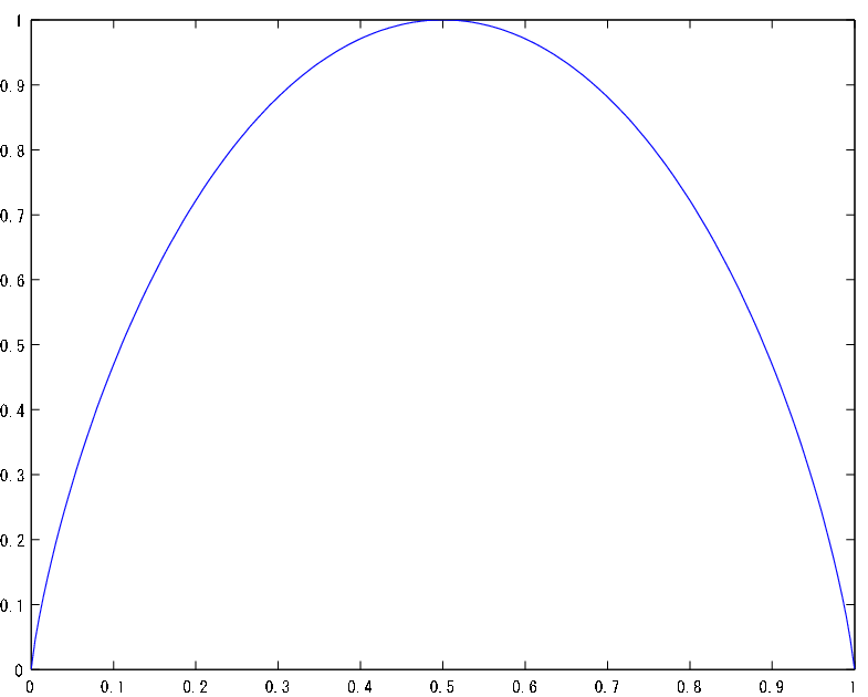
In order to consider the Holevo capacity of a qubit channel, here we consider the von Neumann entropy on the Bloch sphere. The eigenvalues of $\rho(x,y,z)$ (see 29) are $\frac{1+\sqrt{x^{2}+y^{2}+z^{2}}}{2}$ and $\frac{1-\sqrt{x^{2}+y^{2}+z^{2}}}{2}$ , so the von Neumann entropy is the binary entropy of them. The von Neumann entropy on the Bloch sphere is spherically-symmetric and concave function.

5 Relation between $E_{F}$ and the Holevo capacity

Due to Stinespring’s dilation [Stinespring 55] any CPTP map $\Lambda:\mathcal{B}(\mathcal{H}_{\mathtt{in}})\to\mathcal{B}(\mathcal{H}_{\mathtt{out}})$ can be represented as the composition of an isometric embedding³³ 3 A linear operator or map $U$ is called an isometric embedding if $U^{\dagger}U$ is an identity operator. The name isometric embedding emerged from the following two reasons: • Any vector ${|{\phi}\rangle}$ does not change its length after the mapping $U$ , as $\left\|\,{|{\phi}\rangle}\,\right\|=\|\,U{|{\phi}\rangle}\,\|$ . This is because $\|\,{|{\phi}\rangle}\,\|^{2}=\langle\phi|{\phi}\rangle={\langle{\phi}|}U^{\dagger}U{|{\phi}\rangle}=(U{|{\phi}\rangle})^{\dagger}(U{|{\phi}\rangle})=\|\,U{|{\phi}\rangle}|\,\|^{2}$ and $\|\,{|{\phi}\rangle}\,\|\geq 0,\|\,U{|{\phi}\rangle}\,\|\geq 0$ . • Any vectors do not change their distance after the mapping $U$ as $\|\,{|{\phi}\rangle}-{|{\psi}\rangle}\,\|=\|\,U{|{\phi}\rangle}-U{|{\psi}\rangle}\,\|$ . Note that isometric embedding is not always a unitary transformation, even though any unitary transformation is always an isometric embedding. of ${\mathcal{B}(\mathcal{H}_{\mathtt{in}})}$ into a bipartite system $\mathcal{B}(\mathcal{H}_{\mathtt{out}})\otimes\mathcal{B}(\mathcal{H}_{\mathtt{aux}})$ followed by the operation tracing out $\mathcal{B}(\mathcal{H}_{\mathtt{aux}})$ leaving the output space $\mathcal{B}(\mathcal{H}_{\mathtt{out}})$ , represented as,

\Lambda:\quad\begin{aligned} \mathcal{B}({\mathcal{H}_{\mathtt{in}}})&\>\stackrel{{\scriptstyle U}}{{\hookrightarrow}}\>&\>\mathcal{B}(\mathcal{H}_{\mathtt{out}}\otimes\mathcal{H}_{\mathtt{aux}})&\stackrel{{\scriptstyle{\operatorname{Tr}}_{\mathcal{H}_{\mathtt{aux}}}}}{{\longrightarrow}}&\mathcal{B}(\mathcal{H}_{\mathtt{out}})\quad\\ \rho\quad&\>\mapsto&U\rho\>U^{\dagger}\quad&\longmapsto&\quad{\operatorname{Tr}}_{\mathcal{H}_{\mathtt{out}}}U\rho\>U^{\dagger}\end{aligned}

(30)

by choosing $\mathcal{H}_{\mathtt{aux}}$ of which the dimension large enough and the isometric embedding $U$ .

Notation 1.26 ( $\mathcal{K}_{\lambda}$ , image vectors of the isometric embedding)

Denote ${\cal K}_{\Lambda}=U{\mathcal{H}_{\mathtt{in}}}$ , a subspace of $\mathcal{H}_{\mathtt{out}}\otimes\mathcal{H}_{\mathtt{aux}}$ , the image subspace of $U$ where $U$ appeared in (30).

We can say that the channel $\Lambda$ is equivalent to a tracing out operation from ${\cal K}_{\Lambda}$ to the output space $\mathcal{H}_{\mathtt{out}}$ , with an isometric embedding $U$ .

Theorem 1.27 (see [Matsumoto-Shimono-Winter 04])

C(\Lambda)=\sup\{S\bigl({\operatorname{Tr}}_{{\cal H}_{\mathtt{aux}}}\rho\bigr)-E_{F}^{\>\tt out:aux}(\rho):\rho\text{ on }{\cal K}_{\Lambda}\}.

(31)

where $C(\cdot)$ is the Holevo capacity defined in (21).

Notation 1.28 ( $\mathcal{O}_{\lambda}(\subset\mathcal{B}(\mathcal{K}_{\lambda}))$ , preimage matrices of the average output.)

For a given channel, denote as follows:

{\cal O}_{\Lambda}=\mathop{\arg\max}\limits_{\rho\in\mathcal{B}({\cal K}_{\Lambda})}\{S\bigl({\operatorname{Tr}}_{\mathcal{H}_{\mathtt{aux}}}\rho\bigr)-E_{F}^{\>\tt out:aux}(\rho):\rho\text{ on }{\cal K}_{\Lambda}\}.

(32)

Theorem 1.29

If $C(\Lambda\otimes\Lambda^{\prime})=C(\Lambda)+C(\Lambda^{\prime})$ holds, then following holds:

\forall\rho\in{\cal O}_{\Lambda},\forall\rho^{\prime}\in{\cal O}_{\Lambda^{\prime}}\quad E_{F}^{\>\tt out:aux}(\rho\otimes\rho^{\prime})=E_{F}^{\>\tt out:aux}(\rho)+E_{F}^{\>\tt out:aux}(\rho^{\prime}).

(33)

∎

It is interesting whether $C(\Lambda^{\otimes n})=nC(\Lambda)$ holds for a given/every channel $\Lambda$ , because one can conclude whether $E_{F}(\rho^{\otimes n})=nE_{F}(\rho)$ holds by the theorem above. As partial results, following channels are known to satisfy this additivity property:

•

Unital qubit channels⁴⁴ 4 A unital channel is a quantum channel $\Lambda:\mathcal{B}(\mathcal{H}_{\mathtt{in}})\to\mathcal{B}(\mathcal{H}_{\mathtt{out}})$ which maps the maximally mixed state of $\mathcal{H}_{\mathtt{in}}$ to the maximally mixed state of $\mathcal{H}_{\mathtt{out}}$ . The maximally mixed state is defined as $\frac{1}{d}\sum_{i=1}^{d}{|{i}\rangle}\!{\langle{i}|}$ for $\mathcal{B}(\mathbb{C}^{d})$ . , cf. [King 02c, King 02a]
•

Entanglement--breaking channels⁵⁵ 5 An entanglement-breaking channel $\Lambda:\mathcal{B}(\mathcal{H}_{\mathtt{in}})\to\mathcal{B}(\mathcal{H}_{\mathtt{out}})$ is an entanglement breaking channel if it satisfies the following condition. Any output of $\Lambda\otimes\tt{1}:\mathcal{B}(\mathcal{H}_{\mathtt{in}})\otimes\mathcal{B}(\mathcal{H}_{\mathtt{aux}})\to\mathcal{B}(\mathcal{H}_{\mathtt{out}})\otimes\mathcal{B}(\mathcal{H}_{\mathtt{aux}})$ is not entangled between $\mathcal{H}_{\mathtt{out}}$ and $\mathcal{H}_{\mathtt{aux}}$ for any auxiliary space $\mathcal{H}_{\mathtt{aux}}$ . Here $\tt{1}$ is the identity map of $\mathcal{B}(\mathcal{H}_{\mathtt{aux}})$ . , cf. [Shor 02]
•

Arbitrary depolarizing channels King⁶⁶ 6 A channel $\Lambda:\mathcal{B}(\mathcal{H})\to\mathcal{B}(\mathcal{H})$ is an depolarizing channel if it is a unital channel and there exist $s\in\mathbb{R}$ such that $\Lambda(\sigma)-\Lambda(\rho)=s\,(\sigma-\rho)$ , namely, $\Lambda$ is a proportionally shrinking mapping toward the maximally mixed state. , cf. [King 02b]

6 Additivity problems

This section gives issues related to the additivity of $E_{F}$ and to the Holevo capacity.

Definition 1.30 (strong superadditivity of $E_{F}$ )

For a state $\rho$ on $\mathcal{H}_{A1}\otimes\mathcal{H}_{A2}\otimes\mathcal{H}_{B1}\otimes\mathcal{H}_{B2}$ , the inequality of strong superadditivity of $E_{F}$ is defined as,

E_{F}^{\>\sf A:B}(\rho)\geq E_{F}^{\>\sf A:B}(\mathop{\mathrm{Tr}}\nolimits_{2}{\rho})+E_{F}^{\>\sf A:B}(\mathop{\mathrm{Tr}}\nolimits_{1}{\rho}).

(34)

Here $\mathop{\mathrm{Tr}}\nolimits_{2}$ means tracing out the space of ${\mathcal{H}_{A1}\otimes\mathcal{H}_{B1}}$ and $\mathop{\mathrm{Tr}}\nolimits_{1}$ means tracing out the space of ${\mathcal{H}_{A2}\otimes\mathcal{H}_{B2}}$ . See Fig. 9. Note that whether this inequality holds for every case has not yet solved.

Theorem 1.31 ([Matsumoto-Shimono-Winter 04, Shor 04])

The following four propositions are equivalent:

•

The additivity in $E_{F}$ : ${}^{\forall}{(\rho,\sigma)}\>:\>E_{F}(\rho\otimes\sigma)=E_{F}(\rho)+E_{F}(\sigma)$
•

The additivity in the Holevo capacity : ${}^{\forall}{(\Lambda_{1},\Lambda_{2})}\>:\>C(\Lambda_{1}\otimes\Lambda_{2})=C(\Lambda_{1})+C(\Lambda_{2})$
•

The strong superadditivity of $E_{F}$ for any mixed states
•

The strong superadditivity of $E_{F}$ for any pure states

7 Miscellaneous

Here, we fix some conventions, which might otherwise cause confusion.

7.1 Base of logarithm

Throughout this dissertation, the base of logarithm is fixed to two (2) unless the base is specifically indicated. Therefore, $\log 2=1$ . Note that this rule is applied to the logarithm of matrices like $\log\rho$ as well, which effects von Neumann entropy and the quantum divergence and so on.

7.2 Convex and concave

Convexity of a function: a function $f$ is convex when it bends downward, as

f(\lambda x+(1-\lambda)y)\leq\lambda f(x)+(1-\lambda)f(y)\quad\mbox{ for }\quad 0\leq\lambda\leq 1.

(35)

Concavity of a function: a function $f$ is concave when it bends upward, as

f(\lambda x+(1-\lambda)y)\geq\lambda f(x)+(1-\lambda)f(y)\quad\mbox{ for }\quad 0\leq\lambda\leq 1.

(36)

7.3 Tensor products

In this chapter, or in this dissertation, the tensor product is defined for

•

pure states,
•

mixed states,
•

mapping or quantum channels

7.4 The terms level and dimension

In quantum informatics, the terms level and dimension may not be different in nature as one can say a state comes from 2-dimensional space or 2-level system. In this dissertation, however, they may be distinguished in some context, as the level refers to the quantum space and the dimension refers to technical derivation to perform the optimizing calculation for the Holevo capacity.

Endnotes of Chapter 1

$\rho,\sigma$ : mixed quantum states
${\|{\phi}\rangle}$	ket
${\langle{\phi}\|}$	bra
$\mathcal{B}(\mathcal{H})$	the set of mixed states of a given Hilbert space
$\square^{T}$	transpose of a given matrix
$\square^{\dagger}$	conjugate transpose or Hermitian transpose of a given matrix
$\rho(\cdot_{x},\cdot_{y},\cdot_{z})$	Stokes parameterization in the Bloch sphere
$B(\rho,\sigma)$	Bures distance between two states
$F(\rho,\sigma)$	fidelity between two states
$H(\rho\,\|\|\,\sigma)$	quantum divergence, quantum relative entropy
$S(\rho)$	von Neumann entropy of a state
$\cdot,\square$ : a mixed quantum state share by the two sites A and B
$E^{\>\sf A:B}(\cdot)$	reduced von Neumann entropy
$E_{C}^{\>\sf A:B}(\cdot)$	entanglement cost
$E_{D}^{\>\sf A:B}(\cdot)$	entanglement distillation
$E_{F}^{\>\sf A:B}(\cdot)$	entanglement of formation
$E_{N}^{\>\sf A:B}(\cdot)$	logarithm of negativity
$E_{R}^{\>\sf A:B}(\cdot)$	relative entropy of entanglement
$\square^{\Gamma}$	partial transpose of a given matrix
$\Lambda$ : a quantum channel
$C(\Lambda)$	Holevo capacity of a quantum channel
$\bar{C}(\Lambda)$	full capacity of a quantum channel
$\mathcal{K}_{\Lambda}$	image vectors induced by an isometric embedding $U$ of a channel $\Lambda$
$\mathcal{O}_{\Lambda}$	preimage matrices of the average output of $\Lambda$ in $\mathcal{B}(\mathcal{K}_{\Lambda})$

Table 1: Denotations used in this dissertation.

Chapter 2 Introduction to the dissertation

The main body of this dissertation is the author’s researches in quantum information science with a main interest in quantum entanglement, and methodologies of conducting research as well.

Before entering the chapters of the research performed, we are going to depict (i) the background of this dissertation, (ii) how the research was conducted, and (iii) this dissertation’s organization.

8 Background

8.1 Quantum information science

Quantum information science, the consolidation of information science and quantum physics, both of which date back to the first half of the twentieth century, has attracted the interest of many researchers over the last ten years as the invention of efficient algorithms for number factorization⁷⁷ 7 Shor’s algorithm : it solves the factorization in $O(n^{3})$ with $n$ being the number of digits, even though the fastest classical algorithm does it in approximately $O(\exp(n^{2/3}))$ . Note that the former is polynomial and the latter is superpolynomial. [Shor 94], and database search⁸⁸ 8 Grover’s algorithm: it finds the target in a database in size $n$ with the time proportional to $O(n^{1/2})$ . This means the time cost grows only 10 times if the database size grows as much as 100 times. [Grover 96]. There is a characteristic phenomena in quantum physics that is called quantum entanglement, which plays an essential role in quantum computation [Jozsa-Linden 02]. Various quantum protocols were devised using quantum entanglement, such as quantum teleportation⁹⁹ 9 Quantum teleportation: it teleports quantum states to a remote place with classical communication and quantum entanglement between the two sites beforehand. [BBCJPW 93] and quantum superdense coding¹⁰¹⁰ 10 Quantum superdense coding: it transmits 2 bits while sending 1 qubit with prepared quantum entanglement. [Bennett-Wiesner 92].

The author is concerned with the entanglement cost [Bennet-DiVicenzo-Smolin-Wootters 96], and also the Holevo capacity [Holevo 73]. The entanglement cost is one way to quantify the entanglement of a bipartite quantum state, and the Holevo capacity is a classical communication capacity of a given quantum channel. These two different measures are related by [Matsumoto-Shimono-Winter 04] through Stinespring’s dilation theorem as presented in section 5.

8.2 Quantifying entanglement

How to quantify the entanglement of quantum states? Quantum entanglement raise up useful effects on quantum computation/communication mysteriously, thus quantification of entanglement is significant and natural methodology to clarify the mystery.

To measure the usefulness of entanglement, there is a simple way is to compare two entangled pairs. There may be a situation that a pair particles shared by Alice and Bob is more entangled than another pair particles also shared by the two figures because the former pair is more useful to be used in quantum communication, say, sending a message in quantum superdense coding. Then how to compare? An established way is to see the possibility of transformation from a pair to the other through LOCC operation, as LOCC cannot create additional entanglement. If a pair #1 can be transformed into another pair #2 by LOCC, then one can say that #1 is more useful than #2.

[Vidal 99] shows a good theorem for this question for pure states. Two pairs of pure states can be compared by the concept of majorization¹¹¹¹ 11 Majorization: two pairs of pure states ${|{\psi_{1}}\rangle}$ and ${|{\psi_{2}}\rangle}$ are compared as follows: – 1. Let $\{\lambda_{i}\}$ and $\{\mu_{i}\}$ be each of the eigenvalues in descending order of $\mathop{\mathrm{Tr}}\nolimits_{A}{|{\psi_{1}}\rangle}\!{\langle{\psi_{1}}|}$ and $\mathop{\mathrm{Tr}}\nolimits_{A}{|{\psi_{2}}\rangle}\!{\langle{\psi_{2}}|}$ , respectively. – 1. Compare the sequences $\{\lambda_{1},\lambda_{1}+\lambda_{2},\lambda_{1}+\lambda_{2}+\lambda_{3},\ldots\}$ and $\{\mu_{1},\mu_{1}+\mu_{2},\mu_{1}+\mu_{2}+\mu_{3},\ldots\}$ . They are equivalent – when ${|{\psi_{1}}\rangle}$ can be transformed to ${|{\psi_{2}}\rangle}$ by LOCC and – when all of $\lambda_{1}\leq\mu_{1},\lambda_{1}+\lambda_{2}\leq\mu_{1}+\mu_{2},\lambda_{1}+\lambda_{2}+\lambda_{3}\leq\mu_{1}+\mu_{2}+\mu_{3},\ldots$ hold. This method to compare is called majorization. This majorization was the first significant step to measure quantum entanglement.

To quantify quantum entanglement literally in quantity, an asymptotic comparison is conceived. The idea is, for a state $\rho$ , to investigate the possibility to transform $\rho^{\otimes N}$ from/into ${|{\Psi^{-}}\rangle}^{\otimes M}$ by LOCC with large $N$ and $M$ . ${|{\Psi^{-}}\rangle}^{\otimes M}$ is considered to have $M$ ebits. The idea is, if $\rho^{\otimes N_{1}}$ can be transformed into ${|{\Psi^{-}}\rangle}^{\otimes M_{1}}$ then $\rho$ is more than $N_{1}/M_{1}$ ebits, and if $\rho^{\otimes N_{2}}$ can be transformed from ${|{\Psi^{-}}\rangle}^{\otimes M_{2}}$ then $\rho$ is less than $N_{2}/M_{2}$ ebits. The former idea is formalized in entanglement distillation ( $E_{D}$ ) and the latter is formalized in entanglement cost ( $E_{C}$ ) (see (25) and (26) ).

For pure states [Popescu-Rohrlich 97, Vidal 00, Nielsen 00, Donald-Horodecki-Rudolph 02], the entanglement cost and the entanglement distillation coincide each other. For mixed states, they are, however, different. That is, irreversibility occurs in asymptotic transformation through LOCC for mixed bipartite state. Thus quantifying entanglement is not simple for mixed states. Another idea is to put a restrict such as a measure should be additive. There has been devised many measures and the entanglement of formation ( $E_{F}$ ) is also a good candidate to measure entanglement. It is originally defined as a formula (27), and the relation (28) connects it to the entanglement cost. Even though the entanglement distillation seems to break the additivity [Shor-Smolin-Terhal 01], the entanglement cost and the entanglement of formation seem not break the additivity, or it is hard to find such a state $\rho$ that breaks the additivity.

8.3 Channel capacity beyond classical physics

For a classical channel, that is a stochastic mapping from the input alphabets to the output alphabets, there is a sole capacity formalized by Shannon, which gives the supremum quantity of information that is transmitted asymptotically per channel use [Shannon 48]. To determine the capacity for classical case, there are efficient algorithms [Arimoto 72, Blahut 72].

For a quantum channel, there could be many capacities for a channel. An interesting quantity is the Holevo capacity, which was upper-bounded by the Holevo quantity [Holevo 73], and proved to be equal to the Holevo quantity [Holevo 98, Schumacher-Westmoreland 97].

There were proposals to calculate the Holevo capacity for general quantum channels [Osawa-Nagaoka 01, Shor 03]. [Osawa-Nagaoka 01] expands the method of the Arimoto-Blahut algorithm. [Shor 03] made a comment utilizing the column generation method. This dissertation presents seemingly the first algorithm to calculate the Holevo capacity of qubit channels [Hayashi-Imai-Matsumoto-Ruskai-Shimono 04].

The Holevo capacity is a measure which does not allow entanglement among input particles. There is a possibility that allowing entanglement among the input particles might increase the capacity, even though the Shannon capacity keeps the additivity. This problem is formalized as whether $C(\Lambda^{\otimes n})=n\,C(\Lambda)$ for $n=2,3,\dots$ , or $C(\Lambda_{1}\otimes\Lambda_{2})=C(\Lambda_{1})+C(\Lambda_{2})$ holds for arbitrary channels. This additivity was related to the additivity of $E_{F}$ [Matsumoto-Shimono-Winter 04]. Verifying the additivity of the Holevo capacity is an interesting problem, thus numerically calculating the Holevo capacity for high-dimensional case is expected.

9 Research flow of this dissertation

This dissertation is concerned with the problems of quantification of quantum entanglement and the computation of the Holevo capacity. As is written above, quantifying the entanglement of bipartite pure states is almost settled, in that the reduced von Neumann entropy is the sole measure with the appropriate conditions. The appropriate properties here are the reducing property against any non-quantum physical operation (formalized in LOCC), additivity property, and so on.

9.1 Quantifying Entanglement

Quantum states are generally mixed states, as each of them presented in the stochastic mixture of some pure states. Various ways of quantifying the entanglement of a given mixed state are proposed [Bennet-DiVicenzo-Smolin-Wootters 96], such as the entanglement cost ( $E_{C}$ ), the entanglement of formation ( $E_{F}$ ), the entanglement distillation ( $E_{D}$ ), and the relative entropy of entanglement ( $E_{R}$ )¹²¹² 12 The relative entropy of entanglement $E_{R}$ : $E_{R}(\rho)$ is defined as $\min\limits_{\sigma:\mathrm{separable}}H(\rho||\sigma)$ . . For a given $\rho$ , $E_{C}(\rho)$ is the measure of how many the Bell states are needed to construct $\rho$ in the asymptotic sense.¹³¹³ 13 The asymptotic sense here means that $\rho$ is not single to be compared with the Bell states. Rather, $\rho^{\otimes n}$ for large $n$ is compared with $m$ copies of the Bell states, and $\frac{m}{n}$ is considered in the limit of $n,m\to\infty$ . $E_{F}$ is similarly defined, but rather technically. $E_{D}$ of $\rho$ is defined as how many the Bell states can be distilled from $\rho$ .

Naive questions might arise: “Which is the best [in quantifying the entanglement of bipartite mixed states]?”, “What is the appropriateness in measures?”, “Is there only one proper measure?”

A relation

E_{C}(\rho)=\lim_{n\to\infty}\frac{E_{F}(\rho^{\otimes n})}{n}

(37)

was given by [Hayden-Horodecki-Terhal 01], thus the following expectation were brought about:

•

$E_{C}$ could be calculated analytically and/or numerically.
•

The additivity of $E_{F}$ , that is

$E_{F}(\rho^{\otimes n})=^{?}n\,E_{F}(\rho),$ (38)

might holds thus $E_{C}=E_{F}$ holds and $E_{C}$ is calculated rather easily.

If the additivity does not hold, calculating $E_{C}$ is a formidable problem. Calculating

E_{F}(\rho)=\min_{n;p_{1},\dots,p_{n};{|{\phi_{1}}\rangle},\dots,{|{\phi_{n}}\rangle}}\left\{\sum_{i=1}^{n}p_{i}\,E({|{\phi_{i}}\rangle}\!{\langle{\phi_{i}}|})\Bigg|\;{\begin{matrix}n\in\mathbb{N},\hfill\\ \,p_{1},\ldots,p_{n}>0,\,\sum_{i=1}^{n}p_{i}=1,\\ {|{\phi_{1}}\rangle},\ldots,{|{\phi_{n}}\rangle}\text{ are pure states},\\ \sum_{i=1}^{n}p_{i}\,{|{\phi_{i}}\rangle}\!{\langle{\phi_{i}}|}=\rho\hfill\end{matrix}}\right\},

(39)

where $E$ is the reduced von Neumann entropy, is quite an high-dimensional optimization problem, even if the dimension of $\rho$ is quite low such as two or three¹⁴¹⁴ 14 For a bipartite $d$ -dimensional system, $n$ in the formula (39) could reach $d^{2}$ , and each of $\{\phi_{i}\}_{i=1}^{d^{2}}$ is a $d^{2}$ -dimensional vector on the bipartite system on $\mathbb{C}$ , represented in $2d^{2}-1$ parameters in $\mathbb{R}$ , as well as $\{p_{i}\}_{i=1}^{d^{2}}$ being considered $(d^{2}-1)$ -dimensional parameters in $\mathbb{R}$ . One can remove one parameter of a global phase of a quantum system. As a whole, the number of parameters is $(2d^{2}-1)\times d^{2}+(d^{2}-1)-1=2d^{4}-2$ . Then, how to optimize such a high-dimensional problems!? It seems very difficult to calculate $E_{F}$ even for $d=2$ . (See the table below.) Fortunately, [Hill-Wootters 97, Wootters 98] gave an analytical formula for $d=2$ to calculate $E_{F}$ . $d$ (1) 2 3 4 5 6 7 $\dots$ $2d^{4}-2$ (0) 30 160 510 1248 2590 4800 $\dots$ Table 2: The dimensional explosion in computing $E_{F}$ . Still more, $E_{C}$ is a limitation form of this problem.

The first trial of calculating $E_{C}$ for nontrivial case was done for three-level antisymmetric states [Vidal-Dür-Cirac 01]. With the expectation of calculating the first case of $E_{C}$ for nontrivial case, the author gave lower bounds of antisymmetric states [Shimono 02], which appear in Chapter 3. More general form of (38) is

E_{F}(\rho\otimes\sigma)=^{?}E_{F}(\rho)+E_{F}(\sigma).

(40)

The author seem to gave the first specific example [Shimono 03], presented in Chapter 4. Conclusively, the first examples to calculate $E_{C}$ for nontrivial case was done by [Vidal-Dür-Cirac 02], for the mixture of Bell states. $E_{C}$ for three-dimensional antisymmetric states was calculated by [Yura 03], and the result was further expanded to more general antisymmetric case [Matsumoto-Yura 04].

As of the days when $E_{C}$ and $E_{D}$ were proposed [Bennet-DiVicenzo-Smolin-Wootters 96], whether they can be different or not was unknown¹⁵¹⁵ 15 The difference between $E_{C}(\rho)$ and $E_{D}(\rho)$ means some LOCC operations are irreversible (even) in an asymptotic sense. Namely, bulk of the Bell state ${|{\Psi^{-}}\rangle}$ in quantity $E_{C}(\rho)$ may be transformed into bulk of $\rho$ in unit quantity by some LOCC operations, but any LOCC operation cannot retrieve the original quantity of the Bell state (refer to the definition of $E_{C}$ and $E_{D}$ .) . Such states were found by [Horodecki 98] for $3\otimes 3$ -level mixed states. Attempts to find other examples was done by [Vidal-Dür-Cirac 02]. The author of this dissertation also gave examples utilizing the following facts:

•

$E_{F}$ can be calculated through the Holevo capacity [Matsumoto-Shimono-Winter 04].
•

$E_{D}$ is bounded by another easily-calculable quantity called the logarithmic negativity [Vidal-Werner 02] $E_{N}$ , i.e. $E_{D}\leq E_{N}$

This result is presented in Chapter 5.

9.2 Strong superadditivity

There is another quantification called “the relative entropy of entanglement” [Vedral-Plenio-Rippin-Knight 97] denoted $E_{R}$ . It was believed to be additive for a while, however, negated later by finding counterexamples [Vollbrecht-Werner 01].

It seems that determining only one measure is not appropriate because $E_{C}(\rho)>E_{D}(\rho)$ holds for some state $\rho$ (examples is presented in Chapter 5), even though both $E_{C}$ and $E_{D}$ are good candidates to measure quantum entanglement. The additivity is the property $E(\rho\otimes\rho^{\prime})=E(\rho)+E(\rho^{\prime})$ or $E(\rho^{\otimes n})=n\,E(\rho)$ . It is of natural and expected requirement for any kind of “measuring”. As quantum entanglement is the valuable peculiarity from an ordinal classical physical viewpoint, one might like to quantify it like counting money. From a theoretical viewpoint of convenience, if the additivity holds for $E_{F}$ , then $E_{F}=E_{C}$ , which leads to a difficult formula of $E_{C}$ in calculation to a more feasible one calculating $E_{F}$ .

Based on the concept written above, the value of $E_{F}$ and $E_{C}$ for some specific states are tried calculated. For example, the antisymmetric states of bipartite three-level systems are taken up. (These states can be regarded as two particles of fermions in one system, thus consideration of this entanglement might cause practical applications.) In order to try to calculate $E_{C}(\rho)$ where $\rho$ is an antisymmetric state, $E_{F}(\rho^{\otimes 2})$ is calculated. (This work is completed by [Yura 03] as $E_{C}(\rho)=1$ , which means $E_{F}(\rho^{\otimes n})$ for $\forall n\in\mathbb{N}$ is calculated. Furthermore, it is extended to the space of $\mathbb{C}^{d}\otimes(\mathbb{C}^{d})^{\otimes d-2}$ [Matsumoto-Yura 04], as the value is $\log_{2}d-1$ .)

With the theorem of Stinespring dilation, the article of [Matsumoto-Shimono-Winter 04] related the Holevo capacity to $E_{F}$ . Utilizing this fact, the author calculated $E_{F}$ for a $2\otimes 4$ - level system, which shows gaps between $E_{F}$ and $E_{D}$ . To check the additivity of $E_{F}$ in the lowest nontrivial case, the inequality of the strong superadditivity for a twin $2\otimes 2$ -level system¹⁶¹⁶ 16 – Firstly, to consider quantum entanglement for a bipartite system, $2\otimes 2$ is the lowest-dimensional case; for an $n\otimes m$ -level system, $n<2$ or $m<2$ is trivial. – Secondly, to check the additivity, twofold (i.e. ^⊗2) of $2\otimes 2$ is the minimum. Therefore, to check the additivity, the nontrivial lowest case to calculate the quantity of entanglement is $(2\otimes 2)^{\otimes 2}$ dimensional, which becomes 16 dimensional.. Feasibility in calculation of the von Neumann entropy for a 4-level system and calculation of $E_{F}$ for $2\otimes 2$ [Hill-Wootters 97, Wootters 98] is utilized, even though calculating $E_{F}$ seems formidable even for a $2^{2}\!\otimes\!2^{2}$ -level system. However, the inequality of the strong superadditivity is easy to check rather than the additivity check, thus the attempts to check this is performed in Chapter 6.

9.3 The Holevo capacity

As the Stinespring correspondence introduces, the action of any quantum channels (CPTP transformation) is equivalent to the result of the following procedure[Matsumoto-Shimono-Winter 04] (see Fig. 12):
– making a tensor product from the input state and a certain auxiliary state,
– transforming it by a certain unitary operator, and then
– reducing into the space of the output.
$E_{F}$ of the intermediate state is equal to [Matsumoto-Shimono-Winter 04]:

the von Neumann entropy of the average output minus the Holevo capacity.

(41)

Therefore, if we can calculate the Holevo capacity, we can calculate the $E_{F}$ for various states. In this dissertation, given examples are calculated utilizing a mathematical programming package NUOPT [NUOPT] of Mathematical Systems Inc., which is capable of solving large optimization problems, and the convergence in calculation is analyzed.

The Holevo capacity is a classical information capacity of a given memoryless quantum channel. Back to the history, it was formalized and upper-bounded by the Holevo quantity [Holevo 73]. The Holevo capacity was proved to be equal to the Holevo quantity later [Holevo 98, Schumacher-Westmoreland 97], which is defined as,

C(\Lambda)=\max_{\begin{smallmatrix}\\ n;\,\hskip 8.19447pt\hskip 16.38895pt\\ \rho_{1},\rho_{2},\dots,\rho_{n};\,\\ p_{1},p_{2},\dots,p_{n}\phantom{;\,}\end{smallmatrix}\hskip-5.69054pt}S(\sum_{i=1}^{n}p_{i}\,\Lambda\rho_{i})-\sum_{i=1}^{n}p_{i}\,S(\Lambda\rho_{i})

(42)

for a quantum channel $\Lambda:\mathcal{B}(\mathcal{H}_{\mathtt{in}})\to\mathcal{B}(\mathcal{H}_{\mathtt{out}})$ , where $S(\cdot)$ is the von Neumann entropy.

In 1998, another representation was provided as [Ohya-Petz-Watanabe 97]:

C(\Lambda)=\min_{\sigma\in\mathcal{B}(\mathcal{H}_{\mathtt{in}})}\max_{\rho\in\mathcal{B}(\mathcal{H}_{\mathtt{in}})}H(\Lambda\rho\,||\,\Lambda\sigma).

(43)

where $H(\cdot||\cdot)$ is the quantum divergence.

9.3.1 Difficulty in calculation

Both of (42) and (43) contain the optimization operators such as min and max, and the functions to be optimized seem challenging to optimize because:

–

The objective function (42) is convex w.r.t. $(\rho_{i})_{i}$ .

Therefore, it is hard to guarantee that a found local maximum is the global one.

There are, however, feasible ways to calculate the Holevo capacity numerically.¹⁷¹⁷ 17 The calculation was done in 2004 using an existing calculator; quantum computers are not yet available! The objective function of (42) is concave w.r.t. each $p_{i}$ because the first term is concave as $S$ is concave and the second term is linear w.r.t. each $p_{i}$ . Therefore, once every $\rho_{i}$ is fixed, it is easy to find the global maximum by gradual descending. The author employs the methodology of covering with a fine lattice the whole space to specify $(\rho_{i})_{i}$ beforehand for qubit channels (see Fig.13). The finer the lattice becomes, the closer the approximative solution becomes to the actual value.

9.3.2 Results

The results in terms of the Holevo capacity of this dissertation are as follows:

–
The Holevo capacity of qubit channels became possible to calculate 31 years after the formula was proposed.
- –
  $S(\sum_{i=1}^{n}p_{i}\,\Lambda\rho_{i})-\sum_{i=1}^{n}p_{i}\,S(\Lambda\rho_{i})$ is maximized by NUOPT [NUOPT].
  - –
    
    Qubit channels which require four inputs to achieve their Holevo capacity are found.
- –
  The convergence of the optimization calculation is analyzed for
  - –
    
    the algorithm maximizing $S(\sum_{i=1}^{n}p_{i}\,\Lambda\rho_{i})-\sum_{i=1}^{n}p_{i}\,S(\Lambda\rho_{i})$ .

9.4 Additivity issues

Here in this subsection, the additivity issues related with quantum entanglement is described.

[Matsumoto-Shimono-Winter 04] revealed the relation between $E_{F}$ (the entanglement of formation) and the Holevo capacity which shows the additivity dependence between them. This relations became to be called the MSW correspondence, and using this relation, [Shor 04] found additivity equivalence among various problems, including the strong superadditivity of $E_{F}$ .

As aforementined, additivity of measures is important; additivity means that the quantity measured for two objects equals the sum of the quantities for the two measured separately, and this additivity property depends on the measure how to quantify. Back to the topic, whether $E_{F}$ is additive or not is important because the additivity of $E_{F}$ leads the additivity of $E_{C}$ and no one knows whether $E_{F}$ is additive or not. Additionary, other measures of entanglement such as $E_{D}$ (entanglement distillation) and $E_{R}$ (the relative entropy of entanglement) were shown to be non-additive, and researchers may like to find out the measure for quantum entanglement that satisfies the additivity. Parallel to this, they like to find out the capacity of quantum channel that satisfies the additivity, and the Holevo capacity is the strong candidate, even though entanglement between input particles may increase the communication efficienty more than the sum of the communication efficiency using non-entangled particles, but nobody knows whether this capacity holds or not.

The importance of the equivalence properties[Matsumoto-Shimono-Winter 04, Shor 04] is as follows.

If the additivity of $E_{F}$ holds: the strong superadditivity of $E_{F}$ holds, and the additivity of the Holevo capacity holds.

If the additivty of $E_{F}$ does not hold, which means there some two quantum states $\rho$ and $\sigma$ satisfying $E_{F}(\rho\otimes\sigma)<E_{F}(\rho)+E_{F}(\sigma)$ : the strong superadditivyt of $E_{F}$ breaks for some quantum states, and the additivity of the Holevo capacity breaks (for some tow channels $\Lambda_{1}$ and $\Lambda_{2}$ , $C(\Lambda_{1}\otimes\Lambda_{2})>C(\Lambda_{1})+C(\Lambda_{2})$ with the aide of entanglement between input particles of the two channels).

From the viewpoint of this additivity, this dissertation can be seen as follows: Chapter 3 and 4 tried to check whether $E_{F}$ is additive for the limited, highly symmetric states. Chapter 6 and 7 tried to find the witness against the additivty, through trying to find the counterexample against the superadditivity of $E_{F}$ and trying to find the breakage of the Holevo capacity of a certain unordinary channel, respectively.

10 Organization of this dissertation

The organization of this dissertation is as follows:

Part I consists of Chapter 1 and this Chapter 2, mentioning the dissertation’s introductory matters. In Chapter 1, we review the basic notations and the definitions in quantum information theory to be used in subsequent chapters. This Chapter 2 is the introduction for the following main body of this dissertation.

Part II, consisting of Chapters 3, 4, 5 and 6, deals with the topics related to entanglement quantification and its additivity problems. Chapters 3 and 4 deal with the entanglement cost of antisymmetric states. Chapter 5 deals with the gap between $E_{C}$ and $E_{D}$ . Chapter 6 deals with the strong superadditivity.

Part III, consisting of Chapter 7, deals with the topics of calculating the Holevo capacity. The Holevo capacity is a significant quantity defined more than thirty years ago, the numerical calculation is, however, difficult. We present the algorithms to calculate it and application of it.

Part IV, the final part, consist of Chapter 8, summarize this dissertation.

Plenty parts of this dissertation are derivation from journal articles and conference presentations, such as :

Chapter 3 from [Shimono 02], Chapter 4 from [Shimono 03], Chapter 5 from [Matsumoto-Shimono-Winter 04], Chapter 7 from [Hayashi-Imai-Matsumoto-Ruskai-Shimono 04].

Endnotes of Chapter 2

Part II Entanglement

Problems concerning quantification of quantum entanglement are integrated in this part. The first two chapters deal with the problem of the entanglement of formation of antisymmetric states in a $3\otimes 3$ -level system. Next, irreversibility of entanglement is shown through presenting the difference in $E_{F}$ and $E_{D}$ for a mixed $2\otimes 4$ -level system. Lastly, the strong superadditivity for a $(2\otimes 2)^{\otimes 2}$ -level system is numerically verified, which gave circumstantial evidences for the additivity of the entanglement of formation.

Chapters in Part II 3 $\forall\rho\mbox{ on }\mathcal{H}_{-}^{3}:\;E_{C}(\rho)\geq 0.585$ , or $E_{F}(\rho^{\otimes n})\geq 0.585n$ . – Attempts for calculating the $E_{C}$ . 4 $\forall\rho\mbox{ on }\mathcal{H}_{-}^{3}:\;E_{F}(\rho)=1,E_{F}(\rho^{\otimes 2})=2$ . – Checking the additivity in $E_{F}$ . 5 $\exists\rho\mbox{ on }\mathbb{C}^{2}\otimes\mathbb{C}^{4}:\;E_{D}(\rho)<E_{C}(\rho)$ . – The gap shows the irreversibility in LOCC. 6 $\exists\rho\mbox{ on }\left(\mathbb{C}^{2}\otimes\mathbb{C}^{2}\right)^{\otimes 2}:\;E_{F}(\rho)\not\geq E_{F}(\mathop{\mathrm{Tr}}\nolimits_{1}\rho)+E_{F}(\mathop{\mathrm{Tr}}\nolimits_{2}\rho)?$ – Attempts for seeking any counterexample against the strong superadditivity

Chapter 3 Lower Bounds for Entanglement Cost of Antisymmetric States

Calculating $E_{C}$ is quite difficult. A breakthrough has been desired. We paid attention to antisymmetric states. Lower bounds were found even though the exact values were unknown.

This chapter gives a lower bound of the entanglement cost for antisymmetric states of a bipartite $d$ -level system to be $\log_{2}\frac{d}{d-1}$ .

This chapter is a derivation from [Shimono 02].

11 First step toward calculating $E_{C}$

The entanglement cost can be determined by asymptotic behavior of the entanglement formation [Hayden-Horodecki-Terhal 01], but it is regarded to be very difficult to calculate.

This chapter gives a lower bound of the entanglement cost of antisymmetric states for a bipartite $d$ -level system. We prove that all of the eigenvalues of each reduced matrix of any pure state affiliating to $\mathcal{H}_{-}^{\otimes n}$ for general $d$ is not greater than $\left(\frac{d-1}{d}\right)^{n}$ , where $\mathcal{H}_{-}$ is the set of antisymmetric states of a bipartite $d$ -level systems, defined in the following section. This is proved by investigating a CP map $\tilde{{\Lambda}}$ defined in (47).

12 Problem setup

The author makes the following assumptions: $\mathcal{H}_{A}$ and $\mathcal{H}_{B}$ are $d$ -dimensional Hilbert spaces with the basis $D=\{|i\rangle\}_{i=1\ldots d}$ . $\mathcal{H}_{AB}=\mathcal{H}_{A}\otimes\mathcal{H}_{B}$ . For $1\leq i<j\leq d$ ,

|(i,j)\rangle={\displaystyle\frac{|i\rangle_{A}\otimes|j\rangle_{B}-|j\rangle_{A}\otimes|i\rangle_{B}}{\sqrt{2}}}\quad\in\quad\mathcal{H}_{AB}\quad.

$D^{\prime}=\{|(i,j)\rangle\}_{1\leq i\lneqq j\leq d}$ . The antisymmetric space $\mathcal{H}_{-}=\mathop{\mathrm{span}}D^{\prime}\subset H_{AB}$ .

Notation 3.1 (matrices)

For a positive integer $m$ , ${\mathfrak{M}}_{m}$ is a set of $m\times m$ -dimensional matrices with each entry a complex number $\mathbb{C}$ . For a set ${\mathfrak{X}}$ , $\left[a_{ij}\right]_{i,j\in{\mathfrak{X}}}$ is a matrix of which any $(i,j)$ -component specified $a_{ij}$ , and ${\mathfrak{M}}({\mathfrak{X}})=\left\{[a_{ij}]_{i,j\in{\mathfrak{X}}}|\{a_{ij}\}\subset\mathbb{C}\right\}$ is a collection of matrices with each row and column labeled with elements of ${\mathfrak{X}}$ .

Notation 3.2 (partial order between matrices)

The partial order $\leq$ in ${\mathfrak{M}}({\mathfrak{X}})$ is employed as follows: For $X_{1},X_{2}\in{\mathfrak{M}}({\mathfrak{X}})$ , $X_{1}\geq X_{2}\Leftrightarrow X_{2}\leq X_{1}\Leftrightarrow X_{1}-X_{2}\geq 0\Leftrightarrow X_{1}-X_{2}$ is a semi-positive Hermitian matrix.

Definition 3.3 ( ${\Lambda}:{\mathfrak{M}}(D^{\prime})\rightarrow{\mathfrak{M}}(D)$ )

The map ${\Lambda}:{\mathfrak{M}}(D^{\prime})\rightarrow{\mathfrak{M}}(D)$ is defined as follows: First, $X\in{\mathfrak{M}}(D^{\prime})$ , is regarded as an antisymmetric state $\rho_{1}:=\sum_{I,J\in D}X_{IJ}|I\rangle\langle J|\in\mathcal{H}_{-}$ , Then $\rho_{1}$ is reduced into $\mathcal{H}_{A}$ by the operation $\rho_{2}:=\mathop{\mathrm{Tr}}\nolimits\limits_{B}\rho_{1}\in\mathcal{H}_{A}$ , and is converted into the matrix representation $Y\in{\mathfrak{M}}(D)$ with the basis $D$ satisfying $\rho_{2}=\sum_{i,j\in D}Y_{ij}|i\rangle\langle j|$ . This transformation $X\mapsto Y$ is the map ${\Lambda}$ .

The derivations of this map ${\Lambda}$ are investigated in section 13.

Notation 3.4 ( ${\mathfrak{E}}_{ij}^{\mathfrak{X}}$ )

For a set ${\mathfrak{X}}$ and every $i,j\in{\mathfrak{X}}$ , ${\mathfrak{E}}_{ij}^{\mathfrak{X}}\in{\mathfrak{M}}({\mathfrak{X}})$ is a matrix with entry $1$ only at the $(i,j)$ -component and $0$ elsewhere. For example, for ${\mathfrak{X}}=\{1,2,3\}$ , ${\mathfrak{E}}_{1,2}^{\mathfrak{X}}=\left(\begin{smallmatrix}0&1&0\\ 0&0&0\\ 0&0&0\end{smallmatrix}\right)$ .

Thus, $[{\mathfrak{E}}^{\mathfrak{X}}_{IJ}]_{I,J\in{\mathfrak{X}}}$ is

\begin{pmatrix}{\mathfrak{E}}^{\mathfrak{X}}_{11}&{\mathfrak{E}}^{\mathfrak{X}}_{12}&{\mathfrak{E}}^{\mathfrak{X}}_{13}\\ {\mathfrak{E}}^{\mathfrak{X}}_{21}&{\mathfrak{E}}^{\mathfrak{X}}_{22}&{\mathfrak{E}}^{\mathfrak{X}}_{23}\\ {\mathfrak{E}}^{\mathfrak{X}}_{31}&{\mathfrak{E}}^{\mathfrak{X}}_{32}&{\mathfrak{E}}^{\mathfrak{X}}_{33}\end{pmatrix}=\left(\begin{smallmatrix}1&0&0&&0&1&0&&0&0&1\\ 0&0&0&&0&0&0&&0&0&0\\ 0&0&0&&0&0&0&&0&0&0\\ \\ 0&0&0&&0&0&0&&0&0&0\\ 1&0&0&&0&1&0&&0&0&1\\ 0&0&0&&0&0&0&&0&0&0\\ \\ 0&0&0&&0&0&0&&0&0&0\\ 0&0&0&&0&0&0&&0&0&0\\ 1&0&0&&0&1&0&&0&0&1\end{smallmatrix}\right)

when ${\mathfrak{X}}$ is $\{1,2,3\}$ , which will be used in this chapter. This example indicates a $3\times 3$ block matrix with $3\times 3$ matrices, thus it is a $9\times 9$ matrix.

Notation 3.5 ( ${{\Lambda}^{\!(\dagger)}}$ )

${{\Lambda}^{\!(\dagger)}}$ is defined as a map $X\mapsto{\Lambda}(X^{\dagger})$ , i.e. a compound transformation for the map ${\Lambda}$ after the matrix adjoint operation(Hermitian transpose). Note that ${{\Lambda}^{\!(\dagger)}}$ operates on Hermitian matrices, as ${\Lambda}$ operates, i.e. for a Hermitian matrix $X$ , ${{\Lambda}^{\!(\dagger)}}(X)={\Lambda}(X)$ because $X^{\dagger}=X$ .

In this chapter “map” is a map between matrices.

Notation 3.6 (identities)

Let us assume each of ${\mathfrak{M}},{\mathfrak{M}}^{\prime}$ is either of ${\mathfrak{M}}_{m}$ or ${\mathfrak{M}}({\mathfrak{X}})$ . Then $\mathop{\mathrm{id}}\limits_{\mathfrak{M}},\mathop{\mathrm{Id}}\limits_{\mathfrak{M}},\mathop{\mathrm{Id}^{\#}}\limits_{{\mathfrak{M}},{\mathfrak{M}}^{\prime}}$ are denoted as follows: $\mathop{\mathrm{id}}\limits_{\mathfrak{M}}$ is the identity matrix of ${\mathfrak{M}}$ , $\mathop{\mathrm{Id}}\limits_{\mathfrak{M}}$ is the identity map on ${\mathfrak{M}}$ , $\mathop{\mathrm{Id}^{\#}}\limits_{{\mathfrak{M}},{\mathfrak{M}}^{\prime}}$ is the linear map ${\mathfrak{M}}\ni X\mapsto(\mathop{\mathrm{Tr}}\nolimits X)\cdot\mathop{\mathrm{id}}\limits_{\mathfrak{M}}\in{\mathfrak{M}}^{\prime}$ . ${\mathfrak{M}},{\mathfrak{M}}^{\prime}$ will sometimes be dropped, as in $\mathop{\mathrm{id}},\mathop{\mathrm{Id}}$ and $\mathop{\mathrm{Id}^{\#}}$ .

13 Propositions and theorems

Lemma 3.7

For scalars $x$ and $y$ , eigenvalues of $\displaystyle\left(\mathop{\mathrm{Id}}\limits_{{\mathfrak{M}}(D^{\prime})}\otimes\Big(x{\Lambda}+y{{\Lambda}^{\!(\dagger)}}\Big)\right)\left[{\mathfrak{E}}^{D^{\prime}}_{IJ}\right]_{I,J\in D^{\prime}}$ are
$-y,\frac{1}{2}y,\frac{d-1}{2}x+\frac{1}{2}y$ .

Proof.

The matrix considered above is equal to $\Xi:=\left[\Big(x{\Lambda}+y{{\Lambda}^{\!(\dagger)}}\Big){\mathfrak{E}}^{D^{\prime}}_{IJ}\right]_{I,J\in D^{\prime}}$ . For $(i,j),(k,l)\in D^{\prime}$ , ${\Lambda}\left({\mathfrak{E}}^{D^{\prime}}_{(i,j)(k,l)}\right)=\mathop{\mathrm{Tr}}\nolimits\limits_{B}|(i,j)\rangle\langle(k,l)|=\frac{1}{2}\begin{smallmatrix}&{{}_{k}\hskip 16.38895pt{}_{l}}\\ \begin{smallmatrix}{\phantom{|}}{}^{i}\\ {\phantom{|}}{}^{j}\end{smallmatrix}\!\!&\left(\begin{smallmatrix}\delta_{jl}&-\delta_{jk}\\ -\delta_{il}&\delta_{ik}\end{smallmatrix}\right)\\ &\phantom{{{}_{i}\hskip 16.38895pt{}_{l}}}\end{smallmatrix}$ where $\delta$ is the Kronecker’s delta, and ${{\Lambda}^{\!(\dagger)}}\left({\mathfrak{E}}^{D^{\prime}}_{(i,j)(k,l)}\right)=\frac{1}{2}\begin{smallmatrix}&{{}_{i}\hskip 16.38895pt{}_{j}}\\ \begin{smallmatrix}{\phantom{|}}{}^{k}\\ {\phantom{|}}{}^{l}\end{smallmatrix}\!\!&\left(\begin{smallmatrix}\delta_{jl}&-\delta_{il}\\ -\delta_{jk}&\delta_{ik}\end{smallmatrix}\right)\\ &\phantom{{{}_{i}\hskip 16.38895pt{}_{l}}}\end{smallmatrix}$ . Observing the whole matrix $\Xi$ , it is decomposed into the form of the direct sum $\displaystyle\Xi=\frac{y}{2}\Xi_{1}\oplus\left(\frac{x}{2}\Xi_{2}+\frac{y}{2}\Xi_{3}\right)$ where

$\displaystyle\Xi_{1}$	$\displaystyle=$	$\displaystyle\mathop{\bigoplus}\limits^{i,j,k}_{1\leq i<j<k\leq d}\begin{smallmatrix}&{{}_{(i,j)\otimes k}\,{}_{(i,k)\otimes j}\,{}_{(j,k)\otimes i}}\\ \begin{smallmatrix}{\phantom{\|}}{}^{(i,j)\otimes k}\\ {\phantom{\|}}{}^{(i,k)\otimes j}\\ {\phantom{\|}}{}^{(j,k)\otimes i}\end{smallmatrix}\!\!&\left(\begin{matrix}0&1&-1\\ 1&0&1\\ -1&1&0\end{matrix}\right)\\ &\phantom{{{}_{i}\hskip 16.38895pt{}_{l}}}\end{smallmatrix},$
$\displaystyle\Xi_{2}$	$\displaystyle=$	$\displaystyle\mathop{\bigoplus}\limits^{i}_{1\leq i\leq d}\bordermatrix{&&&&&&\cr{\phantom{x}}{}^{(1,i)\otimes i}&1&\cdots&1&-1&\cdots&-1\cr\quad\vdots&\vdots&&\vdots&\vdots&&\vdots\cr{\phantom{x}}{}^{(i-1,i)\otimes i}&1&\cdots&1&-1&\cdots&-1\cr{\phantom{x}}{}^{(i,i+1)\otimes i}&-1&\cdots&-1&1&\cdots&1\cr\quad\vdots&\vdots&&\vdots&\vdots&&\vdots\cr{\phantom{x}}{}^{(i,d)\otimes i}&-1&\cdots&-1&1&\cdots&1},$
$\displaystyle\Xi_{3}$	$\displaystyle=$	$\displaystyle\mathop{\bigoplus}\limits^{i}_{1\leq i\leq d}\bordermatrix{&&&&&&\cr{\phantom{x}}{}^{(1,i)\otimes i}&1&&&&&\cr\quad\vdots&&\ddots&&&0&\cr{\phantom{x}}{}^{(i-1,i)\otimes i}&&&1&&&\cr{\phantom{x}}{}^{(i,i+1)\otimes i}&&&&1&&\cr\quad\vdots&&0&&&\ddots&\cr{\phantom{x}}{}^{(i,d)\otimes i}&&&&&&1}.$

$\frac{y}{2}\Xi_{1}$ has eigenvalues $-y$ and $\frac{y}{2}$ . $\left(\frac{x}{2}\Xi_{2}+\frac{y}{2}\Xi_{3}\right)$ has eigenvalues $\frac{1}{2}y$ and $\frac{d-1}{2}x+\frac{1}{2}y$ .

∎

Lemma 3.8

Let $\lambda({x,y})=\max\{|-y|,|\frac{1}{2}y|,|\frac{d-1}{2}x+\frac{1}{2}y|\}$ . Then

	$\displaystyle\quad\mathop{\mathrm{arg\,min}}\limits^{(x,y)}_{x+y=1}\lambda({x,y})$	$\displaystyle=$	$\displaystyle\left(\frac{1}{d},\frac{d-1}{d}\right)\quad\text{and}$		(44)
	$\displaystyle\min\limits_{x+y=1}\lambda({x,y})$	$\displaystyle=$	$\displaystyle\lambda\left(\frac{1}{d},\frac{d-1}{d}\right)=\frac{d-1}{d}.$		(45)

Notation 3.9 ( $\tilde{\lambda},\tilde{{\Lambda}}$ )

Denote that

	$\displaystyle\tilde{\lambda}$	$\displaystyle=$	$\displaystyle\frac{d-1}{d}\quad\text{and}$		(46)
	$\displaystyle\tilde{{\Lambda}}$	$\displaystyle=$	$\displaystyle\frac{1}{d}{\Lambda}+\frac{d-1}{d}{{\Lambda}^{\!(\dagger)}}.$		(47)

Note that due to the last two lemmas,

-\tilde{\lambda}\mathop{\mathrm{id}}\leq\left(\mathop{\mathrm{Id}}\limits_{{\mathfrak{M}}(D^{\prime})}\otimes\tilde{{\Lambda}}\right)\left[{\mathfrak{E}}^{D^{\prime}}_{IJ}\right]_{I,J\in D^{\prime}}\leq\tilde{\lambda}\mathop{\mathrm{id}},

(48)

i.e. the absolute values of all eigenvalues of the central side are not larger than (46). Note that (47) operates on Hermitian matrices, as ${\Lambda}$ does.

Notation 3.10

${D^{\prime}}^{n}$ indicates the bases index of $\mathcal{H}_{-}^{\otimes n}$ , if $D^{\prime}$ is the bases index of $\mathcal{H}_{-}$ , as it associates the direct sum of the set ${D^{\prime}}$ .

Lemma 3.11

\left(\mathop{\mathrm{Id}}\limits_{{\mathfrak{M}}(D^{\prime})^{\otimes n}}\otimes\left(\tilde{\lambda}^{n}\mathop{\mathrm{Id}^{\#}}-\tilde{{\Lambda}}^{\otimes n}\right)\right)\left[{\mathfrak{E}}^{{D^{\prime}}^{n}}_{IJ}\right]_{I,J\in{D^{\prime}}^{n}}\geq 0.

(49)

Here, $\mathop{\mathrm{Id}^{\#}}$ is a map from ${\mathfrak{M}}(D^{\prime})^{\otimes n}$ to ${\mathfrak{M}}(D)^{\otimes n}$ .

Proof.

The inequality (49) is equivalent to

\Big(\mathop{\mathrm{Id}}\otimes\tilde{\lambda}^{n}\mathop{\mathrm{Id}^{\#}}\Big)\left[{\mathfrak{E}}^{{D^{\prime}}^{n}}_{IJ}\right]\geq\Big(\mathop{\mathrm{Id}}\otimes\tilde{{\Lambda}}^{\otimes n}\Big)\left[{\mathfrak{E}}^{{D^{\prime}}^{n}}_{IJ}\right].

(50)

The following is enough to show the above inequality.

\left\{\begin{array}[]{ll}\mathit{LHS.}&=\tilde{\lambda}^{n}\left[\mathop{\mathrm{Id}^{\#}}\big({\mathfrak{E}}^{{D^{\prime}}^{n}}_{IJ}\big)\right]_{I,J}=\tilde{\lambda}^{n}\left[\delta_{IJ}\mathop{\mathrm{id}}\right]_{I,J}=\tilde{\lambda}^{n}\mathop{\mathrm{id}}\\ \mathit{RHS.}&=\Big(\mathop{\mathop{\mathrm{Id}}^{\otimes n}}\limits_{{\mathfrak{M}}(D^{\prime})}\otimes\tilde{{\Lambda}}^{\otimes n}\Big)\Big(\big[{\mathfrak{E}}^{{D^{\prime}}}_{IJ}\big]{}^{\otimes n}\Big)=\Big(\big(\mathop{\mathrm{Id}}\limits_{{\mathfrak{M}}(D^{\prime})}\otimes\tilde{{\Lambda}}\big)\big[{\mathfrak{E}}^{{D^{\prime}}}_{IJ}\big]\Big)^{\otimes n}\\ &\leq\left(\tilde{\lambda}\mathop{\mathrm{id}}\right)^{\otimes n}=\tilde{\lambda}^{n}\mathop{\mathrm{id}}\qquad(\leq\mbox{ {\it due to }}(\ref{ineq:lambda})\quad).\end{array}\right.

(51)

∎

The last lemma successively induces the next two propositions.

Proposition 3.12

$\;\displaystyle\tilde{\lambda}^{n}\mathop{\mathrm{Id}^{\#}}-\tilde{{\Lambda}}^{\otimes n}$ is a CP map.

This is due to (49) and [Choi 99]. (Any map $\Gamma:{\mathfrak{M}}_{m}\to{\mathfrak{M}}_{n}$ is CP if and only if
$\left(\mathop{\mathrm{Id}}_{{\mathfrak{M}}_{m}}\otimes\Gamma\right)\left[{\mathfrak{E}}_{ij}\right]_{i,j=1\ldots m}=\left[\Gamma\left({\mathfrak{E}}_{ij}\right)\right]_{i,j=1\ldots m}$ is a semi-positive matrix.)

Proposition 3.13

$\displaystyle\;{\Lambda}^{\otimes n}(X)\leq\tilde{\lambda}^{n}\mathop{\mathrm{id}}\;$ for $X\in{\mathfrak{M}}(D^{\prime})^{{\otimes n}}$ if $X\geq 0\;,\;\mathop{\mathrm{Tr}}\nolimits X=1$ .

Proposition 3.13 is applied to the proof of Theorem 3.14.

Theorem 3.14

$E(|\Psi\rangle)\geq n\log_{2}\frac{d}{d-1}$ for any pure state $|\Psi\rangle\in\mathcal{H}_{-}^{\otimes n}$ .

This is because Proposition 3.13 indicates that all eigenvalues of the reduced matrix from any antisymmetric states are less than or equal to $\left(\frac{d}{d-1}\right)^{-n}$ .

Lemma 3.15

$E_{F}(\sigma)\geq n\log_{2}{\frac{d}{d-1}}$ for any density matrix $\sigma$ supported on $\mathcal{H}_{-}^{\otimes n}$ .

Proof.

Note that the entanglement formation is defined as

\displaystyle E_{F}(\rho)=\min_{\bigl(p_{i},|\Phi_{i}\rangle\bigr)_{i}\in\Delta(\rho)}\sum_{i}p_{i}E(\Phi_{i})

(52)

where

\Delta(\rho)=\left\{\bigl(p_{i},|\Phi_{i}\rangle\bigr)_{i}\Big|(p_{i}>0,\|\Phi_{i}\|=1)\forall i,\sum_{i}p_{i}=1,\sum_{i}p_{i}|\Phi_{i}\rangle\langle\Phi_{i}|=\rho\right\}

(53)

is the collection of all possible decompositions of $\rho$ . It is known that all of $|\Phi_{i}\rangle$ induced from $\Delta(\rho)$ satisfy $|\Phi_{i}\rangle\in\mathop{\mathrm{Range}}\nolimits(\rho)$ , where $\mathop{\mathrm{Range}}\nolimits(\rho)$ is the image space of a matrix $\rho$ , which is a collection of $\rho|\psi\rangle$ with $|\psi\rangle$ running over the domain of $\rho$ . Hence

E_{F}(\rho)\geq\min\{E(\Phi)|\Phi\in\mathop{\mathrm{Range}}\nolimits(\rho),\|\Phi\|=1\}.

(54)

The condition of the lemma above implies $\mathop{\mathrm{}}{Range}(\rho)\subseteq H_{-}^{\otimes n}$ , therefore the last theorem implies $E_{F}(\sigma)\geq n$ . ∎

Due to $\displaystyle E_{C}(\rho)=\lim_{n\to\infty}\frac{E_{F}(\rho^{\otimes n})}{n}$ [Hayden-Horodecki-Terhal 01], the entanglement cost is given as follows:

Theorem 3.16

$E_{C}(\sigma)\geq n\log_{2}\frac{d}{d-1}$ for any density matrix $\sigma$ supported on $\mathcal{H}_{-}^{\otimes n}$ .

Corollary 3.17 (The lower bound of the entanglement cost for $\mathcal{H}_{-}$ )

E_{C}(\sigma)\geq\log_{2}\frac{d}{d-1}

(55)

for any density matrix $\sigma$ supported on $\mathcal{H}_{-}$ .

14 Conclusion and discussion

This chapter gave a lower bound of the entanglement cost of antisymmetric states for $d$ -dimensional antisymmetric states as the inequality (55).

Chapter 4 Additivity of Entanglement of Formation of Two Three-Level Antisymmetric States

The additivity of $E_{F}$ is an important problem. The feasible problems to reach a hint of a breakthrough were sought. The author tried the problem of $3\otimes 3$ plus $3\otimes 3$ for antisymmetric states.

This chapter again focuses on antisymmetric states. The author proves the entanglement of formation is additive for any tensor product of two three-dimensional bipartite antisymmetric states.

This chapter is a derivation from [Shimono 02].

15 Antisymmetric states

Let us start with an introduction of the notations and concepts used in this chapter. $\mathcal{H}_{-}$ denotes an antisymmetric Hilbert space, which is a subspace of a bipartite Hilbert space $\mathcal{H}_{AB}=\mathcal{H}_{A}\otimes\mathcal{H}_{B}$ , where both $\mathcal{H}_{A}$ and $\mathcal{H}_{B}$ are three-dimensional Hilbert spaces, spanned by the vectors $\{{|{i}\rangle}\}_{i=1}^{3}$ . $\mathcal{H}_{-}$ is a three-dimensional Hilbert space, spanned by states $\{{|{i,j}\rangle}\}_{ij=23,31,12}\;$ , where the state ${|{i,j}\rangle}$ is defined as $\frac{{|{i}\rangle}{|{j}\rangle}-{|{j}\rangle}{|{i}\rangle}}{\sqrt{2}}$ in this chapter. The space $\mathcal{H}_{-}$ is called antisymmetric because by swapping the position of two particles of states ${|{\psi}\rangle}$ in $\mathcal{H}_{-}$ , we get the state $-{|{\psi}\rangle}$ . $\mathcal{H}_{-}^{\otimes{n}}$ is the tensor product of $n$ copies of $\mathcal{H}_{-}$ . These copies will be distinguished by the upper index as $\mathcal{H}_{-}^{(j)}$ , with $j=1,\ldots,n$ . We assume $\mathcal{H}_{-}^{(j)}$ is an antisymmetric subspace of $\mathcal{H}_{A}^{(j)}\otimes\mathcal{H}_{B}^{(j)}$ .

16 The result and proof sketch

It has been shown in [Vidal-Dür-Cirac 01] that $E_{F}(\rho)=1$ for any mixed state $\rho\in\mathcal{B}({\mathcal{H}_{-}})$ . This result will play the key role in our proof. Here we will prove the following theorem:

Theorem 4.1

E_{F}(\rho_{1}\otimes\rho_{2})=E_{F}(\rho_{1})+E_{F}(\rho_{2})\,\left(=2\right)

(56)

for any ${\rho_{1},\rho_{2}\in\mathcal{B}({\mathcal{H}_{-}})}$ .

Proof.

To prove this theorem, it is sufficient to show that

E_{F}(\rho_{1}\otimes\rho_{2})\geq 2

(57)

since the subadditivity $E_{F}(\rho_{1}\otimes\rho_{2})\leq E_{F}(\rho_{1})+E_{F}(\rho_{2})=2$ is trivial. Indeed, it holds

$\displaystyle E_{F}$	$\displaystyle\!\!\!\!(\rho_{1}\otimes\rho_{2})=\inf\sum p_{i}E({\|{\psi_{i}}\rangle}\!{\langle{\psi_{i}}\|})$	(58)
$\displaystyle\leq$	$\displaystyle\!\!\!\!\inf\sum p_{i}^{(1)}p_{i}^{(2)}E({\|{\psi_{i}^{(1)}}\rangle}\!{\langle{\psi_{i}^{(1)}}\|}\otimes{\|{\psi_{i}^{(2)}}\rangle}\!{\langle{\psi_{i}^{(2)}}\|})$
$\displaystyle=$	$\displaystyle\!\!\!\!\inf\sum p_{i}^{(1)}E({\|{\psi_{i}^{(1)}}\rangle}\!{\langle{\psi_{i}^{(1)}}\|})$
	$\displaystyle+\inf\sum p_{i}^{(2)}E({\|{\psi_{i}^{(2)}}\rangle}\!{\langle{\psi_{i}^{(2)}}\|})$
$\displaystyle=$	$\displaystyle\!\!\!\!E_{F}(\rho_{1})+E_{F}(\rho_{2})$

where $(p_{i}^{(j)},{|{\psi_{i}^{(j)}}\rangle})$ are subject to the condition $\rho_{j}=\sum_{i}p_{i}^{(j)}{|{\psi_{i}^{(j)}}\rangle}\!{\langle{\psi_{i}^{(j)}}|}$ . To prove (57), we raise the following proposition and prove it.

E({|{\psi}\rangle}\!{\langle{\psi}|})\geq 2,\text{ for any pure state }{|{\psi}\rangle}\in{\mathcal{H}_{-}^{\otimes{2}}}.

(59)

Using the Schmidt decomposition¹⁸¹⁸ 18 Any pure state ${|{\psi}\rangle}$ of a bipartite space $\mathcal{H}_{A}\otimes\mathcal{H}_{B}$ can be represented as ${|{\psi}\rangle}=\sum_{i}p_{i}{|{\psi_{i}^{A}}\rangle}\otimes{|{\psi_{i}^{B}}\rangle}$ where ${|{\psi_{i}^{A}}\rangle}$ are orthogonal bases of $\mathcal{H}_{A}$ , ${|{\psi_{i}^{B}}\rangle}$ are orthogonal bases of $\mathcal{B}_{B}$ ., and $\{p_{i}\}_{i}$ is a probability distribution. , the state ${|{\psi}\rangle}$ can be decomposed as follows:

{|{\psi}\rangle}=\sum\limits_{i=1}^{3}\sqrt{p_{i}}\>{|{\psi_{i}^{(1)}}\rangle}\otimes{|{\psi_{i}^{(2)}}\rangle},

(60)

where $p_{1},p_{2},p_{3}>0,\quad p_{1}+p_{2}+p_{3}=1$ , and $\{{|{\psi_{i}^{(j)}}\rangle}\}_{i=1}^{3}$ is an orthonormal basis of the Hilbert space $\mathcal{H}_{-}^{(j)}$ for $j=1,2$ . Note that this Schmidt decomposition is with respect to $\mathcal{H}_{-}^{(1)}:\mathcal{H}_{-}^{(2)}$ , or, $\left(\mathcal{H}_{A}^{(1)}\otimes\mathcal{H}_{B}^{(1)}\right):\left(\mathcal{H}_{A}^{(2)}\otimes\mathcal{H}_{B}^{(2)}\right)$ . It is not $\left(\mathcal{H}_{A}^{(1)}\otimes\mathcal{H}_{A}^{(2)}\right):\left(\mathcal{H}_{B}^{(1)}\otimes\mathcal{H}_{B}^{(2)}\right)$ . Here “:” indicates how to separate the system into two subsystems for the decomposition.

Fact 4.2

If $\{{|{\psi_{i}}\rangle}\}_{i=1}^{3}$ is an orthonormal basis of $\mathcal{H}_{-}$ , then there exists a unitary operator $U$ , acting on both $\mathcal{H}_{A}$ and $\mathcal{H}_{B}$ , such that $U\otimes U$ maps the states ${|{\psi_{1}}\rangle},{|{\psi_{2}}\rangle},{|{\psi_{3}}\rangle}$ into the states ${|{2,3}\rangle},{|{3,1}\rangle},{|{1,2}\rangle}$ , respectively.

The proof appears in the next section.

Because of Fact 4.2, there exist unitary operators $U^{(1)},U^{(2)}$ such that

\begin{split}\big(U^{(1)}&\otimes U^{(1)}\otimes U^{(2)}\otimes U^{(2)}\big){|{\psi}\rangle}\hfill\\ &=\sum\limits_{\begin{smallmatrix}{i,j}\\ {ij=23,31,12}\end{smallmatrix}}\sqrt{p_{ij}}\>{|{i,j}\rangle}\otimes{|{i,j}\rangle}\;,\end{split}

(61)

where $p_{23}=p_{1},\;p_{31}=p_{2},\;p_{12}=p_{3}$ . We denote ${|{\phi^{\prime}}\rangle}$ with the value of (61).

As is written in the following, we use the following fact:

Fact 4.3

E({|{\psi^{\prime}}\rangle}\!{\langle{\psi^{\prime}}|})\geq 2\quad\text{ if }\quad\begin{cases}\quad p_{23},p_{31},p_{12}\geq 0\\ \phantom{p_{1}}p_{23}+p_{31}+p_{12}=1\end{cases}.

(62)

The proof of this fact also appears in the next section.

Local unitary operators do not change the von Neumann reduced entropy. Thus $E({|{\psi}\rangle}\!{\langle{\psi}|})=E({|{\psi^{\prime}}\rangle}\!{\langle{\psi^{\prime}}|})\geq 2$ . Therefore the claim (59) is proven.

The entanglement of formation is defined as

E_{F}(\rho)=\!\!\inf_{[(p_{i},\psi_{i})]_{i}\in{\Delta(\rho)}}\sum_{i}p_{i}E({|{\psi_{i}}\rangle}\!{\langle{\psi_{i}}|})

(63)

with

\Delta(\rho)=\left\{\left[(p_{i},\psi_{i})\right]_{i}\Bigm|\!\!\begin{array}[]{l}\sum_{i}p_{i}=1,p_{i}>0\forall i\\ \sum_{i}p_{i}{|{\psi_{i}}\rangle}\!{\langle{\psi_{i}}|}=\rho,\langle{\psi_{i}}|{\psi_{i}}\rangle=1\forall i\end{array}\right\}

and it is known that all ${|{\psi_{i}}\rangle}$ induced from $\Delta(\rho)$ satisfy ${|{\psi_{i}}\rangle}\in\mathop{\mathrm{Range}}\nolimits(\rho)$ , where $\mathop{\mathrm{Range}}\nolimits(\rho)$ is is the set of $\rho{|{\psi}\rangle}$ with ${|{\psi}\rangle}$ running over the domain of $\rho$ , called the image space of the matrix $\rho$ . Hence

E_{F}(\rho)\geq\inf\left\{E({|{\psi}\rangle}\!{\langle{\psi}|})\bigm|{|{\psi}\rangle}\in\mathop{\mathrm{Range}}\nolimits(\rho),\langle{\psi}|{\psi}\rangle=1\right\}.

(64)

Since $\rho_{1}\otimes\rho_{2}\in\mathcal{B}(\mathcal{H}_{-}^{\otimes{2}})$ and $\mathop{\mathrm{Range}}\nolimits(\rho_{1}\otimes\rho_{2})\subseteq\mathcal{H}_{-}^{\otimes{2}}$ , (57) is proven. Therefore (56) has been shown. ∎

17 Proofs of lemmas in this chapter

The proofs of two facts which appeared in the previous section are provided in this section.

Lemma 4.4

If $\{{|{\psi_{i}}\rangle}\}_{i=1}^{3}\subset\mathcal{H}_{-}$ is an orthonormal basis, there exists a unitary operator $U$ , acting on both $\mathcal{H}_{A}$ and $\mathcal{H}_{B}$ , such that $U\otimes U$ maps the states ${|{\psi_{1}}\rangle},{|{\psi_{2}}\rangle},{|{\psi_{3}}\rangle}$ into the states ${|{2,3}\rangle},{|{3,1}\rangle},{|{1,2}\rangle}$ , respectively.

Proof.

Let us start with some notational conventions. In the following, ${}^{T\!\!}{\Box}$ stands for the transpose of a matrix, ${\phantom{}{}^{\phantom{T}\!\!}}{\Box}^{\dagger}$ stands for taking the complex conjugate of each element of a matrix, and ${\phantom{}{}^{\phantom{T}\!\!}}{\Box}^{\Theta}$ denotes the transformation defined later.

Let $U$ be represented as $\left(\begin{smallmatrix}u_{11}&u_{12}&u_{13}\\ u_{21}&u_{22}&u_{23}\\ u_{31}&u_{32}&u_{33}\end{smallmatrix}\right)$ with respect to the basis ${|{1}\rangle},{|{2}\rangle},{|{3}\rangle}$ . An operator and its matrix representation might be different objects, but we identify $U$ with $\left(\begin{smallmatrix}u_{11}&u_{12}&u_{13}\\ u_{21}&u_{22}&u_{23}\\ u_{31}&u_{32}&u_{33}\end{smallmatrix}\right)$ here for convenience. Lengthy calculations show that when a $9\times 9$ -dimensional matrix $U\otimes U$ is considered as a map from $\mathcal{H}_{-}$ into $\mathcal{H}_{-}$ , it can be represented by the following $3\times 3$ -dimensional matrix, with respect to the basis ${|{2,3}\rangle},{|{3,1}\rangle},{|{1,2}\rangle}$ :

U^{\Theta}:=\begin{pmatrix}u_{22}u_{33}-u_{23}u_{32}&&u_{23}u_{31}-u_{21}u_{33}&&u_{21}u_{32}-u_{22}u_{31}\\ u_{32}u_{13}-u_{33}u_{12}&&u_{33}u_{11}-u_{31}u_{13}&&u_{31}u_{12}-u_{32}u_{11}\\ u_{12}u_{23}-u_{13}u_{22}&&u_{13}u_{21}-u_{11}u_{23}&&u_{11}u_{22}-u_{12}u_{21}\end{pmatrix}.\vskip 0.0pt

Then one can show that

U^{\Theta}\cdot^{\>T\!\!\!\!}U=(\det U)\left(\begin{smallmatrix}1&0&0\\ 0&1&0\\ 0&0&1\end{smallmatrix}\right),\vskip 0.0pt

and multiplying $U^{\dagger}$ from the right in the equation above, one can obtain $U^{\Theta}=(\det U)\cdot U^{\dagger}$ , since $U$ is a unitary matrix, and ${}^{T\!\!\!}U\cdot U^{\dagger}$ is equal to the identity matrix.

Since $\{{|{\psi_{i}}\rangle}\}_{i=1,2,3}$ is an orthonormal basis of $\mathcal{H}_{-}$ , there exists a unitary operator on $\mathcal{H}_{-}$ such that ${|{\psi_{1}}\rangle}\mapsto{|{2,3}\rangle},{|{\psi_{2}}\rangle}\mapsto{|{3,1}\rangle},{|{\psi_{3}}\rangle}\mapsto{|{1,2}\rangle}$ . Denote $\Theta_{\psi}$ the corresponding matrix with respect to the basis $\{{|{i,j}\rangle}\}_{ij=23,31,12}$ .

Let $U_{\psi}:={({\det\Theta_{\psi}})^{\frac{1}{2}}}\cdot{\Theta_{\psi}^{\dagger}}$ .¹⁹¹⁹ 19 In the definition above, it does not matter which of the two roots of $\det\Theta_{\psi}$ are taken. It holds that $U_{\psi}^{\Theta}=\Theta_{\psi}$ .²⁰²⁰ 20 Indeed, $U_{\psi}^{\Theta}=(\det U_{\psi}){U_{\psi}^{\dagger}}=(\det\Theta_{\psi})^{\frac{3}{2}}\det\Theta_{\psi}^{\dagger}\cdot({(\det\Theta_{\psi})^{\frac{1}{2}}})^{\dagger}\Theta_{\psi}=\Theta_{\psi}$ . Note that $\det U_{\psi}=\det(\det(\Theta_{\psi})^{\frac{1}{2}}\,\Theta_{\psi}^{\dagger})=(\det\Theta_{\psi})^{\frac{3}{2}}\det\Theta_{\psi}^{\dagger}$ because $\Theta_{\psi}^{\dagger}$ is a $3\times 3$ matrix. Therefore $U_{\psi}\otimes U_{\psi}=U^{\prime}_{\psi}$ . The operator $U_{\psi}$ is the one needed to satisfy the statement of Lemma 4.2. ∎

Lemma 4.5

E({|{\psi^{\prime}}\rangle}\!{\langle{\psi^{\prime}}|})\geq 2\quad\text{ if }\quad\left\{\begin{array}[]{l}{|{\psi^{\prime}}\rangle}=\sum\limits^{i,j}_{ij=23,31,12}\sqrt{p_{ij}}\>{|{i,j}\rangle}{|{i,j}\rangle}\\ p_{23},p_{31},p_{12}\geq 0\\ p_{23}+p_{31}+p_{12}=1\end{array}\right..

Proof.

Let $p_{32}:=p_{23},p_{13}:=p_{31},p_{21}:=p_{12}$ . Then it holds,

$\displaystyle{\|{\psi^{\prime}}\rangle}$	$\displaystyle=$	$\displaystyle\sum^{i,j}_{1\leq i<j\leq 3}\sqrt{p_{ij}}\>{\|{i,j}\rangle}{\|{i,j}\rangle}\vskip-17.07164pt$
	$\displaystyle=$	$\displaystyle\frac{1}{{2}}\sum^{i,j}_{1\leq i<j\leq 3}\sqrt{p_{ij}}\>\{{\|{ii;jj}\rangle}-{\|{ij;ji}\rangle}-{\|{ji;ij}\rangle}+{\|{jj;ii}\rangle}\}\vskip-17.07164pt$
	$\displaystyle=$	$\displaystyle\frac{1}{{2}}\sum^{i,j}_{1\leq i\neq j\leq 3}\sqrt{p_{ij}}\>\{{\|{ii;jj}\rangle}-{\|{ij;ji}\rangle}\},\vskip 0.0pt$

where ${|{i_{1}i_{2};i_{3}i_{4}}\rangle}$ denotes the tensor product ${|{i_{1}}\rangle}\otimes{|{i_{2}}\rangle}\otimes{|{i_{3}}\rangle}\otimes{|{i_{4}}\rangle}$ , where ${|{i_{1}}\rangle}\in\mathcal{H}_{A}^{(1)}$ , ${|{i_{2}}\rangle}\in\mathcal{H}_{A}^{(2)}$ , ${|{i_{3}}\rangle}\in\mathcal{H}_{B}^{(1)}$ and ${|{i_{4}}\rangle}\in\mathcal{H}_{B}^{(2)}$ , and the condition $1\leq i\neq j\leq 3$ actually means “ $1\leq i\leq 3$ , $1\leq j\leq 3$ and $i\neq j$ ”.

We are now going to calculate the reduced matrix of ${|{\psi^{\prime}}\rangle}\!{\langle{\psi^{\prime}}|}$ , denoted $\Xi$ , and decomposed into the direct sum as follows:

$\displaystyle\Xi$	$\displaystyle:=$	$\displaystyle\mathop{\mathrm{Tr}}\limits_{\mathcal{H}_{B}^{(1)}\otimes\mathcal{H}_{B}^{(2)}}{\|{\psi^{\prime}}\rangle}{\langle{\psi^{\prime}}\|}$	(65)
	$\displaystyle=$	$\displaystyle\frac{1}{4}\sum^{i,j,k,l}_{\begin{smallmatrix}{1\leq i\neq j\leq 3}\\ {1\leq k\neq l\leq 3}\end{smallmatrix}}\sqrt{p_{ij}p_{kl}}\mathop{\mathrm{Tr}}\limits_{\mathcal{H}_{B}^{(1)}\otimes\mathcal{H}_{B}^{(2)}}\left({\begin{matrix}{{\|{ii;jj}\rangle}{\langle{kk;ll}\|}-{\|{ii;jj}\rangle}{\langle{kl;lk}\|}\phantom{abc}}\\ {\phantom{abc}-{\|{ij;ji}\rangle}{\langle{kk;ll}\|}+{\|{ij;ji}\rangle}{\langle{kl;lk}\|}}\end{matrix}}\right)$
	$\displaystyle=$	$\displaystyle\frac{1}{4}\sum^{i,j,k,l}_{\begin{smallmatrix}{1\leq i\neq j\leq 3}\\ {1\leq k\neq l\leq 3}\end{smallmatrix}}\sqrt{p_{ij}p_{kl}}\mathop{\mathrm{Tr}}\limits_{\mathcal{H}_{B}^{(1)}\otimes\mathcal{H}_{B}^{(2)}}\big({{{\|{ii;jj}\rangle}{\langle{kk;ll}\|}+{\|{ij;ji}\rangle}{\langle{kl;lk}\|}}}\big)$
	$\displaystyle=$	$\displaystyle\frac{1}{4}\sum^{i,j,k}_{\begin{smallmatrix}{1\leq i\neq j\leq 3}\\ {1\leq k\neq l\leq 3}\end{smallmatrix}}\sqrt{p_{ik}p_{jk}}\>{\|{ii}\rangle}{\langle{jj}\|}+\frac{1}{4}\sum^{i,j}_{{1\leq i\neq j\leq 3}}{p_{ij}}\>{\|{ij}\rangle}{\langle{ij}\|}$
	$\displaystyle\cong$	$\displaystyle\frac{1}{4}\left(\begin{smallmatrix}p_{12}+p_{13}&\sqrt{p_{13}p_{23}}&\sqrt{p_{12}p_{23}}\\ \sqrt{p_{13}p_{23}}&p_{12}+p_{23}&\sqrt{p_{12}p_{13}}\\ \sqrt{p_{12}p_{23}}&\sqrt{p_{12}p_{13}}&p_{13}+p_{23}\end{smallmatrix}\right)\oplus\frac{1}{4}(p_{12})^{\oplus 2}\oplus\frac{1}{4}(p_{13})^{\oplus 2}\oplus\frac{1}{4}(p_{23})^{\oplus 2},$

where $\oplus$ denotes the direct sum of matrices, and $\Box^{\oplus n}$ denotes the direct sum of $n$ copies of same matrices.

We need to get the eigenvalues of $\Xi$ in order to calculate the reduced von Neumann entropy $E({|{\psi^{\prime}}\rangle}\!{\langle{\psi^{\prime}}|})=-\mathop{\mathrm{Tr}}\nolimits\left(\Xi\log_{2}\Xi\right)=-\!\!\sum\limits_{\lambda:\mathrm{e.v.of}\;\Xi}\!\!\lambda\,\log_{2}\lambda.$ In this case, fortunately, the whole eigenvalues can be determined explicitly from (65):

\left\{\frac{1-\cos\theta}{6},\frac{1-\cos(\theta+\frac{2\pi}{3})}{6},\frac{1-\cos(\theta+\frac{4\pi}{3})}{6},\frac{p_{12}}{4},\frac{p_{12}}{4},\frac{p_{13}}{4},\frac{p_{13}}{4},\frac{p_{23}}{4},\frac{p_{23}}{4}\right\}

(66)

for a certain $-\frac{\pi}{3}<\theta\leq\frac{\pi}{3}$ .²¹²¹ 21 The exact value of $\theta$ has no importance for us in the proof. The eigenvalues above are denoted as $\{\lambda_{1},\lambda_{2},\ldots,\lambda_{9}\},$ respectively. Although $\lambda_{4},\dots,\lambda_{9}$ are trivial, $\lambda_{1},\lambda_{2},\lambda_{3}$ are the roots of the cubic polynomial

g(\lambda):=\lambda^{3}-\frac{1}{2}\lambda^{2}+\frac{1}{16}\lambda-\frac{p_{12}\>p_{13}\>p_{23}}{16},

(67)

that is the characteristic polynomial function of the cubic matrix that appeared in (65). We must solve this cubic equation to obtain (66). The cubic equation $g(\lambda)=0$ is a Cardan’s irreducible form,²²²² 22 A cubic equation is said to be in Cardan’s irreducible form if its three roots are real numbers. because $\Xi$ is a density matrix. In such a case, the roots of the cubic equation are

\alpha+\beta\cos\theta,\alpha+\beta\cos(\theta+\frac{2\pi}{3}),\alpha+\beta\cos(\theta+\frac{4\pi}{3}).\vskip 0.0pt

(68)

One can easily show that $\lambda_{1}+\lambda_{2}+\lambda_{3}=3\alpha,$ and $\lambda_{1}^{2}+\lambda_{2}^{2}+\lambda_{3}^{2}=3\alpha^{2}+\frac{3}{2}\beta^{2}$ . If $\lambda_{1},\lambda_{2},\lambda_{3}$ are equal to the roots of the cubic equation $\lambda^{3}+a_{1}\lambda^{2}+a_{2}\lambda+a_{3}=0$ , then $\lambda_{1}+\lambda_{2}+\lambda_{3}=-a_{1}$ and $\lambda_{1}^{2}+\lambda_{2}^{2}+\lambda_{3}^{2}=a_{1}^{2}-2a_{2}$ hold. Taking $a_{1}=-\frac{1}{2},a_{2}=\frac{1}{16}$ from (67), we get the simultaneous equations $\{3\alpha=\frac{1}{2},3\alpha^{2}+\frac{3}{2}\beta^{2}=\frac{1}{8}\}$ , with one of the solutions $(\alpha,\beta)=\left(\frac{1}{6},-\frac{1}{6}\right)$ . Applying this argument to (68), we complete (66).

The author’s idea is now to show that

E({|{\psi^{\prime}}\rangle}\!{\langle{\psi^{\prime}}|})=\sum_{i=1}^{9}(-\lambda_{i}\log_{2}\lambda_{i})\geq 2.\vskip 0.0pt

(69)

This will be shown if we prove that the following:

\sum_{i=1}^{3}(-\lambda_{i}\log_{2}\lambda_{i})\geq 1\quad\text{ and }\quad\sum_{i=4}^{9}(-\lambda_{i}\log_{2}\lambda_{i})\geq 1.\vskip 0.0pt

(70)

The second inequality is easy to verify by simple calculations. Therefore, to finish the proof of the lemma we need to show that

\sum_{i=1}^{3}(-\lambda_{i}\log_{2}\lambda_{i})\geq 1.

(71)

Without loss of generality, one can assume $\theta\in\left[0,\frac{\pi}{3}\right]$ .²³²³ 23 The set of $\{\lambda_{i}\}_{i=1}^{3}$ does not change if $\theta$ is replaced by $-\theta$ . Thus we can change the assumption $\theta\in\left(-\frac{\pi}{3},\frac{\pi}{3}\right]$ into $\theta\in\left[0,\frac{\pi}{3}\right]$ . Clearly, $\lambda_{1}\in\left[0,\frac{1}{12}\right]$ and $\lambda_{2},\lambda_{3}=\frac{1}{4}-\frac{\lambda_{1}\pm\sqrt{\lambda_{1}-3\lambda_{1}^{2}}}{2}\in\left[\frac{1}{12},\frac{1}{3}\right]$ . ( $\lambda_{2},\lambda_{3}$ can be regarded as the solution of the following simultaneous equations: $\lambda_{1}+\lambda_{2}+\lambda_{3}=\frac{1}{2},\lambda_{1}^{2}+\lambda_{2}^{2}+\lambda_{3}^{2}=\frac{1}{8}$ . ) One can also show that

-z\log_{2}z\geq\begin{cases}\phantom{ab}(\log_{2}12)\>z&\text{ if $z\in\left[0,\frac{1}{12}\right]$}\\ \phantom{ab}\frac{1}{2}+\frac{\log_{e}4-1}{\log_{e}2}(z-\frac{1}{4})-4(z-\frac{1}{4})^{2}&\text{ if $z\in\left[\frac{1}{12},\frac{1}{3}\right]$}\end{cases}

(72)

(see Fig.1).

The first inequality of (72) is easily confirmed. One way to prove the second inequality is as follows: Let $f(z):=\bigl(-z\log_{2}z\bigr)-\left(\frac{1}{2}+\frac{\log_{e}4-1}{\log_{e}2}(z-\frac{1}{4})-4(z-\frac{1}{4})^{2}\right)$ . Differentiating this expression with respect to $z$ once and twice respectively, we can get the increasing and decreasing table as Table. 3.

$z$	$\frac{1}{12}$		$\frac{1}{8\log_{e}2}$		$\frac{1}{4}$
$f(z)$	$+$	$\curvearrowright$	$+$	$\searrow$	$0$	$\nearrow$
$f^{\prime}(z)$				$-$	$0$	$+$
$f^{\prime\prime}(z)$		$-$	$0$	$+$	$+$	$+$

Table 3: The increase/decrease table of

\bigl(-z\log_{2}z\bigr)-\left(\frac{1}{2}+\frac{\log_{e}4-1}{\log_{e}2}(z-\frac{1}{4})-4(z-\frac{1}{4})^{2}\right)

The table indicates $f(z)\geq 0$ for $z\in\left[\frac{1}{12},\frac{1}{3}\right]$ . Now we indeed get the lower bounds with polynomial functions.

Combining all of the above inequalities, we get (71) as

-\sum\limits_{i=1}^{3}\lambda_{i}\log_{2}\lambda_{i}\geq 1+\left(\frac{\log_{e}3+2}{\log_{e}2}-2\right)\lambda_{1}+4\lambda_{1}^{2}\geq 1\quad.

Therefore (70) and (69) are successively shown, and our proof is completed. ∎

18 Conclusion and discussion

The additivity of the entanglement of formation for two three-dimensional bipartite antisymmetric states has been proven in this paper.

Endnotes

Chapter 5 A Gap Between $E_{F}$ and $E_{D}$

Are there gaps between $E_{D}$ and $E_{C}$ ? That was an important problem. The answer was yes. We found such examples for a $2\otimes 4$ -level system in 2004, after the bound entanglement for a $3\otimes 3$ -level system was found [Horodecki 98] in Poland.

This chapter is a derivation from [Matsumoto-Shimono-Winter 04].

19 Background

The problem is stated as follows:

Is there a gap between the two important and not-yet-fully-analyzed quantities of quantum entanglement presented below?

1.

$E_{C}(\rho)$ , the entanglement cost,
— the asymptotic quantity of Bell states needed to produce $\rho$ under LOCC operation,

2.

$E_{D}(\rho)$ , the entanglement distillation,
— the asymptotic quantity of Bell states retrieved from $\rho$ under LOCC operation.

If there is no difference, meaning $E_{C}(\rho)=E_{D}(\rho)$ for any $\rho$ , the problem of quantification of quantum entanglement may end up easy to handle. That the equality holds for pure states is already known [Popescu-Rohrlich 97, Vidal 00, Nielsen 00, Donald-Horodecki-Rudolph 02] thus the problem resides for $\rho$ being non-pure state. If there is a difference, which means $E_{C}(\rho)>E_{D}(\rho)$ ²⁴²⁴ 24 $E_{C}(\rho)<E_{D}(\rho)$ does not occur for any $\rho$ in principle. If it did, quantum entanglement would increase infinitely by LOCC operations. , one can say the irreversibility occurred under LOCC operation and that the degradation of quantum entanglement is inevitable.

Analyzing this problem is theoretically interesting when investigating the property of quantum entanglement.

Here is a historical note. There are already answers in that there exists such $\rho$ that satisfy $E_{D}(\rho)<E_{C}(\rho)$ . The first examples are such states $\rho$ that satisfy $E_{C}(\rho)>0$ and $E_{D}(\rho)=0$ , which are named bound entanglement [Horodecki 98]. The bound entanglement appears in a $3\otimes 3$ -level system. Other attempts are performed at [Vidal-Dür-Cirac 01] for antisymmetric states. This chapter gives the examples of a $2\otimes 4$ -level system, with mathematical software Maple, through calculating the Holevo capacity of unital channels [King 02c].

20 Introduction

We need to estimate both the values of $E_{C}$ and $E_{D}$ . $E_{C}$ can be calculated by the Holevo capacity if the full capacity $\bar{C}$ is determined through Stinespring’s relation because of the relation between $E_{F}$ and the Holevo capacity (see Sec. 5). To evaluate the value of $E_{D}$ there is a useful estimation theorem.

Notation 5.1 (the logarithmic negativity)

The logarithmic negativity $E_{N}$ of $\rho$ where $\rho$ is shared by two sites is defined as follows:

E_{N}(\rho)=\log\sum_{i}|\lambda_{i}|

(73)

where $\{\lambda_{i}\}$ are the eigenvalues of $\rho^{\Gamma}$ where $\rho^{\Gamma}$ is the partial transpose of $\rho$ . The partial transpose of a state for a bipartite system is defined as $(a_{i\otimes j,k\otimes l})_{(i\otimes j),(k\otimes l)}\mapsto(a_{k\otimes j,i\otimes l})_{(i\otimes j),(k\otimes l)}$ .

Theorem 5.2 ([Vidal-Werner 02])

E_{D}(\rho)\leq E_{N}(\rho)

(74)

Note that $E_{N}$ is simple to calculate even though the method to calculate $E_{D}$ for general cases is not known.

Therefore, the aforementioned gap $E_{D}(\rho)<E_{C}(\rho)$ is concluded, if

–

$E_{C}(\rho)$ is calculated and
–

$E_{N}(\rho)<E_{C}(\rho)$ is determined,

by some method.

21 Unital channel and its associated state

We considered a generalized depolarizing channel²⁵²⁵ 25 A depolarizing channel and a generalized depolarizing channel: – A depolarizing channel for a qubit is a channel with its output ellipsoid being a sphere and its center located at the center of the Bloch sphere. ( The output ellipsoid is explained in Subsection 4.2. ) – A generalized depolarizing channel here is defined as follows: a qubit channel is a generalized depolarizing channel as long as the center of its output ellipsoid is located at the center of the Bloch sphere. The output ellipsoid of the generalized depolarizing channel of (75) has three axes in $x,y,z$ directions with the radius of $p_{0}+p_{x}-p_{y}-p_{z},p_{0}+p_{y}-p_{x}-p_{z}$ and $p_{0}+p_{z}-p_{x}-p_{y}$ .

Figure 18: An illustration of the Bloch sphere and the output ellipsoid of a general depolarizing channel. With the condition (77), the longest axis is

z

-directional. on a qubit:

\Lambda:\rho\longmapsto\sum_{s=0,x,y,z}p_{s}\,\sigma_{s}\rho\sigma_{s}^{\dagger},

(75)

with the Pauli matrices

\sigma_{0}=\left(\begin{array}[]{rr}1&0\\ 0&1\end{array}\right),\ \sigma_{x}=\left(\begin{array}[]{rr}0&1\\ 1&0\end{array}\right),\ \sigma_{y}=\left(\begin{array}[]{rr}0&-\sqrt{-1}\\ \sqrt{-1}&0\end{array}\right),\ \sigma_{z}=\left(\begin{array}[]{rr}1&0\\ 0&-1\end{array}\right),\

and a probability distribution $\{p_{s}\}_{s=0,x,y,z}$ .

There is an interesting theorem about the additivity of the Holevo capacity for depolarizing channel:

Theorem 5.3 ([King 02a])

For generalized depolarizing channels, additivity of the Holevo capacity in terms of tensor product with an arbitrary channel holds. Namely,

C(\Lambda\otimes\Lambda^{\prime})=C(\Lambda)+C(\Lambda^{\prime})

(76)

for any generalized depolarizing channel $\Lambda$ and any channel $\Lambda^{\prime}$ .

Note that up to unitary transformations on the input and the output systems, each unital qubit channel has this form [King-Ruskai 01, Fujiwara-Algoet 99].

We assume the condition

p_{0}+p_{z}-p_{x}-p_{y}\geq|p_{0}+p_{y}-p_{x}-p_{z}|,|p_{0}+p_{x}-p_{y}-p_{z}|,

(77)

which does not lose generality. Then for such a channel $\Lambda$ the capacity is given by

C(\Lambda)=1-S_{\rm min}(\Lambda)

(78)

where $S_{\rm min}(\Lambda)$ is the minimum output entropy of $\Lambda$ , which is achieved at either of the inputs ${|{0}\rangle},{|{1}\rangle}$ , thus $S_{\rm min}(\Lambda)=S\bigl(\Lambda({|{0}\rangle}\!{\langle{0}|})\bigr)=S\bigl(\Lambda({|{1}\rangle}\!{\langle{1}|})\bigr)$ . The optimal ensemble of input signals of the channel in order to achieve the Holevo capacity is the uniform distribution $(1/2,1/2)$ on the two states ${|{0}\rangle},{|{1}\rangle}$ .

A Stinespring dilation for this map $\Lambda:\mathcal{B}(\mathcal{H}_{\tt i})\to\mathcal{B}(\mathcal{H}_{\tt o})$ is given by an isometric embedding $U:\mathcal{H}_{\mathtt{i}}\longrightarrow\mathcal{H}_{\mathtt{o}}\otimes\mathcal{H}_{\mathtt{a}}$ where $\mathcal{H}_{\mathtt{i}},\mathcal{H}_{\mathtt{o}}={\mathbb{C}}^{2}$ and $\mathcal{H}_{\mathtt{a}}={\mathbb{C}}^{4}$ , in the following $8\times 4$ block form:

U=\left(\begin{array}[]{r}\sqrt{p_{0}}\sigma_{0}\\ \sqrt{p_{x}}\sigma_{x}\\ \sqrt{p_{y}}\sigma_{y}\\ \sqrt{p_{z}}\sigma_{z}\end{array}\right),

(79)

and the corresponding subspace ${\cal K}\subset\mathcal{H}_{\mathtt{o}}\otimes\mathcal{H}_{\mathtt{a}}$ is spanned by

	$\displaystyle{\|{\psi_{\Lambda}}\rangle}$	$\displaystyle=\sqrt{p_{0}}{\|{0}\rangle}\otimes{\|{0}\rangle}+\sqrt{p_{x}}{\|{1}\rangle}\otimes{\|{x}\rangle}+\sqrt{-1}\sqrt{p_{y}}{\|{1}\rangle}\otimes{\|{y}\rangle}+\sqrt{p_{z}}{\|{0}\rangle}\otimes{\|{z}\rangle},$		(80)
	$\displaystyle{\|{\psi_{\Lambda}^{\perp}}\rangle}$	$\displaystyle=\sqrt{p_{0}}{\|{1}\rangle}\otimes{\|{0}\rangle}+\sqrt{p_{x}}{\|{0}\rangle}\otimes{\|{x}\rangle}-\sqrt{-1}\sqrt{p_{y}}{\|{0}\rangle}\otimes{\|{y}\rangle}-\sqrt{p_{z}}{\|{1}\rangle}\otimes{\|{z}\rangle}.$		(81)

(You can easily verify that $\Lambda$ is equal to the operation $\rho\mapsto\mathop{\mathrm{Tr}}\nolimits_{\mathcal{H}_{\mathtt{a}}}U\rho U^{\dagger}$ .) The average of the optimal input state²⁶²⁶ 26 Consider the definition of the Holevo capacity: $C(\Lambda)=\max_{n;\rho_{1},\dots,\rho_{n};p_{1},\dots,p_{n}}S(\sum_{i=1}^{n}p_{i}\,\Lambda\rho_{i})-\sum_{i=1}^{n}p_{i}\,S(\Lambda\rho).$ We call the optimized $\{\rho_{i}\}_{i}$ the optimal input. The average input is $\sum_{i}p_{i}\rho_{i}$ . is transformed to the equal mixture of the two pure states

\rho_{\Lambda}=\frac{1}{2}{|{\psi_{\Lambda}}\rangle}\!{\langle{\psi_{\Lambda}}|}+\frac{1}{2}{|{\psi_{\Lambda}^{\perp}}\rangle}\!{\langle{\psi_{\Lambda}^{\perp}}|}

(82)

by $U$ .

With Theorem 1.27, (78) leads to

E_{F}^{\>\tt o:a}(\rho_{\Lambda})=S_{\rm min}(\Lambda)=H(p_{0}+p_{z},p_{x}+p_{y})

(83)

where $H$ is the entropy function and $E_{F}^{\>\tt o:a}(\rho_{\Lambda}\otimes\sigma)=E_{F}^{\>\tt o:a}(\rho_{\Lambda})+E_{F}^{\>\tt o:a}(\sigma)$ for any $\sigma\in{\cal O}_{\Lambda^{\prime}}$ , with an arbitrary channel $\Lambda^{\prime}$ . Theorem 1.29 leads to $E_{F}^{\>\tt o:a}(\rho_{\Lambda}^{\otimes n})=nE_{F}^{\>\tt o:a}(\rho)$ , thus

E_{C}^{\>\tt o:a}(\rho_{\Lambda})=H(p_{0}+p_{z},p_{x}+p_{y}).

(84)

This leads to that the decomposition of $\rho_{\Lambda}^{\otimes n}$ into the $2^{n}$ equally-weighted tensor products of ${|{\psi_{\Lambda}}\rangle}\!{\langle{\psi_{\Lambda}}|}$ , ${|{\psi_{\Lambda}^{\perp}}\rangle}\!{\langle{\psi_{\Lambda}^{\perp}}|}$ being is formation--optimal²⁷²⁷ 27 The formation–optimal here means that the collection of states gives the optimal value of (1.24), which is the formula of the entanglement of formation.. By the convex roof property of $E_{F}$ this implies that any convex combination of these states is a formation–optimal decomposition. (This argument was also used in [Vollbrecht-Werner 01] to extend the domain of states with known entanglement of formation.) In particular, we can conclude that

E_{C}^{\>\tt o:a}(\rho)=E_{F}^{\>\tt o:a}(\rho)=H(p_{0}+p_{z},p_{x}+p_{y})

(85)

for any mixture $\rho$ of ${|{\psi_{\Lambda}}\rangle}\!{\langle{\psi_{\Lambda}}|}$ and ${|{\psi_{\Lambda}^{\perp}}\rangle}\!{\langle{\psi_{\Lambda}^{\perp}}|}$ .

— We may omit the superscription ( ${}^{\>\tt o:a}\>$ ) from here.

22 A gap between $E_{C}$ and $E_{D}$

One can verify that the partial transpose $\rho_{\Lambda}^{\Gamma}$ of the optimal state $\rho_{\Lambda}$ is decomposed into a form of the direct sum of two $4\times 4$ –matrices from (82), which have the same characteristic equation

	$\displaystyle f(2t)$	$\displaystyle=0,\ \text{ with}$		(86)
	$\displaystyle f(t)$	$\displaystyle=t^{4}-t^{3}+4(p_{0}p_{x}p_{y}+p_{0}p_{x}p_{z}+p_{0}p_{y}p_{z}+p_{x}p_{y}p_{z})t-16p_{0}p_{x}p_{y}p_{z}.$		(87)

This equation $f\left(2t\right)=0$ has only one negative root denoted $t_{0}$ , and $f$ is decreasing in a neighborhood of $t_{0}$ . See Fig. 19.

Assume $\rho_{\Lambda}^{\Gamma}$ has eigenvalues $\{t_{0},t_{0},t_{1},t_{1},t_{2},t_{2},t_{3},t_{3}\}$ . Since $t_{0}+t_{0}+t_{1}+t_{1}+t_{2}+t_{2}+t_{3}+t_{3}=1$ , $\left\|\rho_{\Lambda}^{\Gamma}\right\|_{1}=|t_{0}|+|t_{0}|+|t_{1}|+|t_{1}|+|t_{2}|+|t_{2}|+|t_{3}|+|t_{3}|=|2t_{0}|+|2t_{1}+2t_{2}+2t_{3}|=(-2t_{0})+(1-2t_{0})=1-4t_{0}$ , where $\|\cdot\|_{1}$ is one-norm, or the sum of the abstract value of the eigenvalues. Hence $E_{N}(\rho_{\Lambda})=\log(1-4t_{0})$ . Thus $E_{N}(\rho_{\Lambda})<E_{C}(\rho_{\Lambda})$ is successively equivalent to $\log(1-4t_{0})<H(p_{0}+p_{z},p_{x}+p_{y})$ , $1-4t_{0}<2^{H(p_{0}+p_{z},p_{x}+p_{y})}$ , $\frac{1-2^{H(p_{0}+p_{z},p_{x}+p_{y})}}{2}<2t_{0}$ , and

f\left(-\frac{2^{H(p_{0}+p_{z},p_{x}+p_{y})}-1}{2}\right)>0.

(88)

This means if $p_{0}$ , $p_{x}$ , $p_{y}$ , $p_{z}$ satisfy this inequality (88), there is a gap between the entanglement cost of $\rho_{\Lambda}$ , and its entanglement distillation, namely $E_{D}(\rho_{\Lambda})<E_{C}(\rho_{\Lambda})$ ; Fig. 20 shows the plot of the region of these $(p_{x},p_{y},p_{z})$ . Due to this continuity, also for a mixture of ${|{\psi_{\Lambda}}\rangle}\!{\langle{\psi_{\Lambda}}|}$ and ${|{\psi_{\Lambda}^{\perp}}\rangle}\!{\langle{\psi_{\Lambda}^{\perp}}|}$ which is sufficiently close to $\rho_{\Lambda}$ , we observe a similar gap.

Example 5.4

Assume $(p_{0},p_{x},p_{y},p_{z})=(\frac{1}{2},\frac{1}{6},\frac{1}{6},\frac{1}{6})$ . Then $E_{D}(\rho_{\Lambda})<E_{C}(\rho_{\Lambda})$ .

Proof.

A short calculation reveals that $\left\|\rho_{\Lambda}^{\Gamma}\right\|_{1}=5/3$ , so $E_{D}(\rho_{\Lambda})\leq\log(5/3)\approx 0.737$ , which is smaller than the entanglement cost $E_{C}(\rho_{1})=H(1/3,2/3)\approx 0.918$ .

You can also verify that LHS of (88) is $0.00784$ (which is larger than 0), thus $E_{D}(\rho_{\Lambda})<E_{C}(\rho_{\Lambda})$ . ∎

In this case,

\rho_{\Lambda}={\left(\ \begin{matrix}\frac{1}{4}&0&0&\frac{-\sqrt{-1}}{4\sqrt{3}}&\vline&0&\frac{1}{4\sqrt{3}}&\frac{1}{4\sqrt{3}}&0\\ 0&\frac{1}{12}&\frac{-\sqrt{-1}}{4\sqrt{3}}&0&\vline&\frac{-\sqrt{-1}}{12}&0&0&\frac{\sqrt{-1}}{12}\\ 0&\frac{\sqrt{-1}}{4\sqrt{3}}&\frac{1}{4}&0&\vline&\frac{1}{4\sqrt{3}}&0&0&\frac{-1}{4\sqrt{3}}\\ \frac{\sqrt{-1}}{4\sqrt{3}}&0&0&\frac{1}{12}&\vline&0&\frac{\sqrt{-1}}{12}&\frac{\sqrt{-1}}{12}&0\\ \hline\cr 0&\frac{\sqrt{-1}}{12}&\frac{1}{4\sqrt{3}}&0&\vline&\frac{1}{12}&0&0&\frac{-1}{12}\\ \frac{1}{4\sqrt{3}}&0&0&\frac{-\sqrt{-1}}{12}&\vline&0&\frac{1}{12}&\frac{1}{12}&0\\ \frac{1}{4\sqrt{3}}&0&0&\frac{-\sqrt{-1}}{12}&\vline&0&\frac{1}{12}&\frac{1}{12}&0\\ 0&\frac{-\sqrt{-1}}{12}&\frac{-1}{4\sqrt{3}}&0&\vline&\frac{-1}{12}&0&0&\frac{1}{12}\\ \end{matrix}\ \right)}\in\mathcal{B}(\mathcal{H}_{\sf o})\otimes\mathcal{B}(\mathcal{H}_{\sf a})

(89)

Example 5.5

Assume $(p_{0},p_{x},p_{y},p_{z})=(\frac{u}{2},\frac{1-v}{2},\frac{v}{2},\frac{1-u}{2})$ with $u,v\in[0,\frac{1}{2})\cup(\frac{1}{2},1]$ . Then $E_{D}(\rho_{\Lambda,s})<E_{C}(\rho_{\Lambda,s})$ holds for $\rho_{\Lambda,s}=s{|{\psi_{\Lambda}}\rangle}\!{\langle{\psi_{\Lambda}}|}+(1-s){|{\psi_{\Lambda}^{\perp}}\rangle}\!{\langle{\psi_{\Lambda}^{\perp}}|}$ with $0\leq s\leq 1$ . In this case, $\rho_{\Lambda,s}$ is an $8\times 8$ matrix with variables $s,u,v$ , represented as

{\frac{1}{2}\left(\ \begin{matrix}su&0&0&s\sqrt{uu^{\prime}}&\vline&0&-s\sqrt{-uv^{\prime}}&s\sqrt{uv}&0\\ 0&s^{\prime}v&s^{\prime}\sqrt{-vv^{\prime}}&0&\vline&s^{\prime}\sqrt{uv}&0&0&-s^{\prime}\sqrt{u^{\prime}v}\\ 0&-s^{\prime}\sqrt{-vv^{\prime}}&s^{\prime}v^{\prime}&0&\vline&-s^{\prime}\sqrt{-uv^{\prime}}&0&0&s^{\prime}\sqrt{-u^{\prime}v^{\prime}}\\ s\sqrt{uu^{\prime}}&0&0&su^{\prime}&\vline&0&-s\sqrt{-u^{\prime}v^{\prime}}&s\sqrt{u^{\prime}v}&0\\ \hline\cr 0&s^{\prime}\sqrt{uv}&s^{\prime}\sqrt{-uv^{\prime}}&0&\vline&s^{\prime}u&0&0&-s^{\prime}\sqrt{uu^{\prime}}\\ s\sqrt{-uv^{\prime}}&0&0&s\sqrt{-u^{\prime}v^{\prime}}&\vline&0&sv^{\prime}&s\sqrt{-vv^{\prime}}&0\\ s\sqrt{uv}&0&0&s\sqrt{u^{\prime}v}&\vline&0&-s\sqrt{-vv^{\prime}}&sv&0\\ 0&-s^{\prime}\sqrt{u^{\prime}v}&-s^{\prime}\sqrt{-u^{\prime}v^{\prime}}&0&\vline&-s^{\prime}\sqrt{uu^{\prime}}&0&0&s^{\prime}u^{\prime}\end{matrix}\ \right)}

(90)

where $s^{\prime}=1-s,u^{\prime}=1-u,v^{\prime}=1-v$ .

Proof.

By eq. (85), $E_{C}(\rho_{\Lambda,s})=1$ . The key observation is whether $\log\|\rho_{\Lambda}^{\Gamma}\|_{1}<E_{C}(\rho_{\Lambda,s})$ . This is true because the condition (88) is always satisfied, as LHS of (88) is $\frac{1}{2}(u-\frac{1}{2})^{2}+\frac{1}{2}(v-\frac{1}{2})^{2}-(u-\frac{1}{2})^{2}(v-\frac{1}{2})^{2}$ which is zero at $(u,v)=(\frac{1}{2},\frac{1}{2})$ ; it is also an increasing function w.r.t. both $\tilde{u}=(u-\frac{1}{2})^{2}$ and $\tilde{v}=(v-\frac{1}{2})^{2}$ for $\tilde{u},\tilde{v}\leq\frac{1}{4}$ (See Fig. 21).

∎

23 Conclusion and discussion

We have found the states which show the gap as $E_{D}(\rho)<E_{C}(\rho)$ for a $2\otimes 4$ -level system. They were found by analyzing general depolarizing channels with Stinespring’s dilation. This discovery also shows a usefulness of the relationship between $E_{F}$ and the Holevo capacity (see Section 5) found by [Matsumoto-Shimono-Winter 04]. The examples shown in this chapter are the lowest dimensional cases among those bipartite states $\rho$ being proved $E_{D}(\rho)<E_{C}(\rho)$ , in that they are 8 dimensional ( $2\otimes 4$ ), though the next lowest cases are the bound entanglement which are 9 dimensional ( $3\otimes 3$ ) found in earlier in [Horodecki 98]. Our research may exemplify that analyzing the entanglement even in the easiest cases would involve variant ideas such as quantum channels that are tied to entanglement by Stinespring’s relation.

Endnotes

Chapter 6 Numerical Verification of Superadditivity

The strong superadditivity of $E_{F}$ is rather simple to check among the equivalent additivity problems. The author numerically checked the lowest-dimensional cases, which are described as “ $2\otimes 2$ plus $2\otimes 2$ ”.

In this chapter, the strong superadditivity of the entanglement of formation is numerically verified. This is a part of attempts to verify the expects that the whole additivity holds for the entanglement of formation (see Sec 6). It is interesting because if there were any single counterexample against the strong superadditivity, the expected relation $E_{F}\equiv E_{C}$ and the additivity of the Holevo capacities would collapse. The additivity of the minimum entropy of channels would also collapse [Shor 04].

As a result, any single counterexample has been found from approximately a million randomly-chosen cases and various directive searches. Even though this is a negative result, it gave the knowledge that finding counterexamples is a challenging problem even if they exist.

24 Introduction

The strong superadditivity of the entanglement of formation for four-partite qubits is numerically checked in this chapter. The strong superadditivity is represented by the inequality defined in Section 6, as

\qquad\qquad E_{F}(\rho)\geq E_{F}(\mathop{\mathrm{Tr}}\nolimits_{1}\rho)+E_{F}(\mathop{\mathrm{Tr}}\nolimits_{2}\rho)\\ \quad\mbox{ for }\quad\rho\quad\mbox{ on }\quad\mathcal{H}_{A1}\otimes\mathcal{H}_{A2}\otimes\mathcal{H}_{B1}\otimes\mathcal{H}_{B2}.\qquad\qquad

(91)

The additivity of entanglement of formation can be deduced directly from this superadditivity if this inequality (91) holds for any pure case [Matsumoto-Shimono-Winter 04].

In this chapter $\mathcal{H}_{A1},\mathcal{H}_{A2},\mathcal{H}_{B1}$ and $\mathcal{H}_{B2}$ are assumed to be a two-level systems (four qubits). There are several reasons. First of all, this is the lowest-dimensional case. Second, there are feasible method to numerically calculate the values appeared in (91):

•

The left hand side of (91) is just a von Neumann entropy when $\rho$ is a pure state.
•

Each term of the right hand side of (91) is feasible to calculate by the method of the concurrence [Hill-Wootters 97, Wootters 98] when the argument is as low as two-dimensional.

Note that direct calculation of $E_{F}$ is formidable as it is defined as an optimization form on high-dimensional space as it is defined as (1.24).

Furthermore, there is another reason to check the inequality rather than to check the additivity. Technically, inequality check is easier than equality check. You cannot stop concerning about the calculation accuracy when you check the equality numerically, whereas you can when you are checking the inequality numerically unless the equality exactly holds.

25 Calculation procedure for the inequality

In this section, we show the procedure how to numerically verify (91) for a chosen case. This is the base of the experiment executed millions times, which works for $\mathcal{H}_{A_{1}},\mathcal{H}_{B_{1}},\mathcal{H}_{A_{2}},\mathcal{H}_{B_{2}}$ being 2-level systems.

(1) Start from a four-partite qubit pure state that is represented as sixteen-dimensional vector $\begin{split}|\Psi_{A_{1}B_{1}A_{2}B_{2}}\rangle=\sum_{i,j,k,l=0}^{1}\alpha_{ijkl}\,|i\rangle_{A_{1}}|j\rangle_{B_{1}}|k\rangle_{A_{2}}|l\rangle_{B_{2}}\hskip 18.49988pt\\ =(\alpha_{0000}\,\alpha_{0001}\,\ldots\,\alpha_{1110}\,\alpha_{1111}\,)^{T}\end{split}$ (92) for a randomly chosen 16-tuple of complex numbers $\{\alpha_{ijkl}\}$ with the normalized restriction $\sum_{i,j,k,l=0}^{1}|\alpha_{ijkl}|^{2}=1.$

$\downarrow$

(2) Calculate three reduced density operators, $\rho_{A_{1}A_{2}}$ , $\rho_{A_{1}B_{1}}$ and $\rho_{A_{2}B_{2}}$ from ${|{\Psi_{A_{1}B_{1}A_{2}B_{2}}}\rangle}\!{\langle{\Psi_{A_{1}B_{1}A_{2}B_{2}}}|}$ , as $\displaystyle\rho_{A_{1}A_{2}}=\mathop{\mathrm{Tr}}\nolimits_{B_{1}B_{2}}{|{\Psi_{A_{1}B_{1}A_{2}B_{2}}}\rangle}\!{\langle{\Psi_{A_{1}B_{1}A_{2}B_{2}}}|},$ (93) $\displaystyle\rho_{A_{1}B_{1}}=\mathop{\mathrm{Tr}}\nolimits_{A_{2}B_{2}}{|{\Psi_{A_{1}B_{1}A_{2}B_{2}}}\rangle}\!{\langle{\Psi_{A_{1}B_{1}A_{2}B_{2}}}|},$ (94) $\displaystyle\rho_{A_{2}B_{2}}=\mathop{\mathrm{Tr}}\nolimits_{A_{1}B_{2}}{|{\Psi_{A_{1}B_{1}A_{2}B_{2}}}\rangle}\!{\langle{\Psi_{A_{1}B_{1}A_{2}B_{2}}}|}.$ (95) They are $4\times 4$ matrices. Assume they are represented as $\left[\begin{smallmatrix}0&1&2&3\\ 4&5&6&7\\ 8&9&A&B\\ C&D&E&F\end{smallmatrix}\right]$ . Then each symbol $0,1,\ldots,F$ is the summation of the elements of $\rho_{A_{2}B_{2}}=\mathop{\mathrm{Tr}}\nolimits_{A_{1}B_{2}}{|{\Psi_{A_{1}B_{1}A_{2}B_{2}}}\rangle}\!{\langle{\Psi_{A_{1}B_{1}A_{2}B_{2}}}|}$ positioned by the same four letters as follows. (93),(94),(95) for
$\left[\begin{smallmatrix}0&.&1&.&.&.&.&.&2&.&3&.&.&.&.&.\\ .&0&.&1&.&.&.&.&.&2&.&3&.&.&.&.\\ 4&.&5&.&.&.&.&.&6&.&7&.&.&.&.&.\\ .&4&.&5&.&.&.&.&.&6&.&7&.&.&.&.\\ .&.&.&.&0&.&1&.&.&.&.&.&2&.&3&.\\ .&.&.&.&.&0&.&1&.&.&.&.&.&2&.&3\\ .&.&.&.&4&.&5&.&.&.&.&.&6&.&7&.\\ .&.&.&.&.&4&.&5&.&.&.&.&.&6&.&7\\ 8&.&9&.&.&.&.&.&A&.&B&.&.&.&.&.\\ .&8&.&9&.&.&.&.&.&A&.&B&.&.&.&.\\ C&.&D&.&.&.&.&.&E&.&F&.&.&.&.&.\\ .&C&.&D&.&.&.&.&.&E&.&F&.&.&.&.\\ .&.&.&.&8&.&9&.&.&.&.&.&A&.&B&.\\ .&.&.&.&.&8&.&9&.&.&.&.&.&A&.&B\\ .&.&.&.&C&.&D&.&.&.&.&.&E&.&F&.\\ .&.&.&.&.&C&.&D&.&.&.&.&.&E&.&F\\ \end{smallmatrix}\right]\!\!,\!\!\left[\begin{smallmatrix}0&.&.&.&1&.&.&.&2&.&.&.&3&.&.&.\\ .&0&.&.&.&1&.&.&.&2&.&.&.&3&.&.\\ .&.&0&.&.&.&1&.&.&.&2&.&.&.&3&.\\ .&.&.&0&.&.&.&1&.&.&.&2&.&.&.&3\\ 4&.&.&.&5&.&.&.&6&.&.&.&7&.&.&.\\ .&4&.&.&.&5&.&.&.&6&.&.&.&7&.&.\\ .&.&4&.&.&.&5&.&.&.&6&.&.&.&7&.\\ .&.&.&4&.&.&.&5&.&.&.&6&.&.&.&7\\ 8&.&.&.&9&.&.&.&A&.&.&.&B&.&.&.\\ .&8&.&.&.&9&.&.&.&A&.&.&.&B&.&.\\ .&.&8&.&.&.&9&.&.&.&A&.&.&.&B&.\\ .&.&.&8&.&.&.&9&.&.&.&A&.&.&.&B\\ C&.&.&.&D&.&.&.&E&.&.&.&F&.&.&.\\ .&C&.&.&.&D&.&.&.&E&.&.&.&F&.&.\\ .&.&C&.&.&.&D&.&.&.&E&.&.&.&F&.\\ .&.&.&C&.&.&.&D&.&.&.&E&.&.&.&F\\ \end{smallmatrix}\right]\!\!,\!\!\left[\begin{smallmatrix}0&1&2&3&.&.&.&.&.&.&.&.&.&.&.&.\\ 4&5&6&7&.&.&.&.&.&.&.&.&.&.&.&.\\ 8&9&A&B&.&.&.&.&.&.&.&.&.&.&.&.\\ C&D&E&F&.&.&.&.&.&.&.&.&.&.&.&.\\ .&.&.&.&0&1&2&3&.&.&.&.&.&.&.&.\\ .&.&.&.&4&5&6&7&.&.&.&.&.&.&.&.\\ .&.&.&.&8&9&A&B&.&.&.&.&.&.&.&.\\ .&.&.&.&C&D&E&F&.&.&.&.&.&.&.&.\\ .&.&.&.&.&.&.&.&0&1&2&3&.&.&.&.\\ .&.&.&.&.&.&.&.&4&5&6&7&.&.&.&.\\ .&.&.&.&.&.&.&.&8&9&A&B&.&.&.&.\\ .&.&.&.&.&.&.&.&C&D&E&F&.&.&.&.\\ .&.&.&.&.&.&.&.&.&.&.&.&0&1&2&3\\ .&.&.&.&.&.&.&.&.&.&.&.&4&5&6&7\\ .&.&.&.&.&.&.&.&.&.&.&.&8&9&A&B\\ .&.&.&.&.&.&.&.&.&.&.&.&C&D&E&F\\ \end{smallmatrix}\right]$ ,
respectively.

$\downarrow$

(3) Calculate the $E_{F}$ for a pure state $|\Psi_{A_{1}B_{1}A_{2}B_{2}}\rangle$ , as $\displaystyle E_{F}(|\Psi_{A_{1}B_{1}A_{2}B_{2}}\rangle\langle\Psi_{A_{1}B_{1}A_{2}B_{2}}|)=S(\rho_{A_{1}A_{2}}),$ (96) where $S(\rho_{A_{1}A_{2}})$ is the von Neumann entropy that is calculated by the Shannon entropy $-\sum\lambda_{i}\log\lambda_{i}$ with $\{\lambda_{i}\}_{i}$ the eigenvalues of the reduced density operator $\rho_{A_{1}A_{2}}$ that is a $4\times 4$ matrix. Thus one need to solve a quartic equation (a polynomial of order four) or utilize some mathematical package to calculate the eigenvalues of matrices.

$\downarrow$

(4) Calculate the ’spin-flip’ transformations [Wootters 98] of the reduced density operators, $\tilde{\rho}_{A_{1}B_{1}}$ and $\tilde{\rho}_{A_{2}B_{2}}$ by calculating $\displaystyle\tilde{\rho}_{A_{1}B_{1}}$ $\displaystyle=$ $\displaystyle(\sigma_{y}\otimes\sigma_{y})\rho^{T}_{A_{1}B_{1}}(\sigma_{y}\otimes\sigma_{y}),$ (97) $\displaystyle\tilde{\rho}_{A_{2}B_{2}}$ $\displaystyle=$ $\displaystyle(\sigma_{y}\otimes\sigma_{y})\rho^{T}_{A_{2}B_{2}}(\sigma_{y}\otimes\sigma_{y}).$ (98) $\sigma_{y}=\left(\begin{smallmatrix}0&-\sqrt{-1}\\ \sqrt{-1}&0\end{smallmatrix}\right)$ is one of the Pauli matrices. Thus $\sigma_{y}\otimes\sigma_{y}=\left(\begin{smallmatrix}0&0&0&-1\\ 0&0&1&0\\ 0&1&0&0\\ -1&0&0&0\end{smallmatrix}\right)$ . This spin-flip transformation $\rho\mapsto\tilde{\rho}$ is the operation like $\left[\begin{smallmatrix}0&1&2&3\\ 4&5&6&7\\ 8&9&A&B\\ C&D&E&F\end{smallmatrix}\right]\mapsto\left[\begin{smallmatrix}\ F&-E&-D&\ C\\ -B&\ A&\ 9&-8\\ -7&\ 6&\ 5&-4\\ \ 3&-2&-1&\ 0\end{smallmatrix}\right]$ .

$\downarrow$

(5) Calculate the concurrence of $\rho_{A_{1}B_{1}}$ and $\rho_{A_{2}B_{2}}$ by the following calculations: first calculate the square roots of the eigenvalues of $\rho_{A_{1}B_{1}}\tilde{\rho}_{A_{1}B_{1}}$ and arrange them in decreasing order $\lambda_{1},\lambda_{2},\lambda_{3},\lambda_{4}$ ; next, calculate the concurrence $\displaystyle C(\rho_{A_{1}B_{1}})=\max\{0,\lambda_{1}-\lambda_{2}-\lambda_{3}-\lambda_{4}\}.$ (99) Do the same for $\rho_{A_{2}B_{2}}$ , as $C(\rho_{A_{2}B_{2}})=\max\{0,\mu_{1}-\mu_{2}-\mu_{3}-\mu_{4}\}$ (100) where $\mu_{1},\mu_{2},\mu_{3},\mu_{4}$ are the eigenvalues of $\rho_{A_{2}B_{2}}\tilde{\rho}_{A_{2}B_{2}}$ arranged in decreasing order.

$\downarrow$

(6) Calculate $E_{F}$ for $\rho_{A_{1}B_{1}}$ and $\rho_{A_{2}B_{2}}$ by $\displaystyle E_{F}(\rho_{A_{1}B_{1}})=H_{2}\left(\frac{1-\sqrt{1-C(\rho_{A_{1}B_{1}})^{2}}}{2}\right),$ (101) $\displaystyle E_{F}(\rho_{A_{2}B_{2}})=H_{2}\left(\frac{1-\sqrt{1-C(\rho_{A_{2}B_{2}})^{2}}}{2}\right),$ (102) where $H_{2}$ is the binary entropy function.
( $E_{F}(\rho)=-\frac{1-\sqrt{1-C(\rho)^{2}}}{2}\log_{2}\frac{1-\sqrt{1-C(\rho)^{2}}}{2}-\frac{1+\sqrt{1-C(\rho)^{2}}}{2}\log_{2}\frac{1+\sqrt{1-C(\rho)^{2}}}{2}$ )

$\downarrow$

(7) Compare the values $\displaystyle E_{F}({|{\Psi_{A_{1}B_{1}A_{2}B_{2}}}\rangle}\!{\langle{\Psi_{A_{1}B_{1}A_{2}B_{2}}}|})\hskip 9.24994pt\leq^{??}\hskip 9.24994ptE_{F}(\rho_{A_{1}B_{1}})+E_{F}(\rho_{A_{2}B_{2}}),$ (103) to check whether the superadditivity of $E_{F}$ holds or not.

26 Procedure to pick up random points and their results

Three different methods are performed to pick up points, which are then substituted into the procedure described in the section above.

26.1 Random search

Sixteen parameters $z_{ijkl}\,(i,j,k,l=0,1)$ are chosen from uniformly from the square whose four vertices are $\pm 1\pm\sqrt{-1}$ on the Gaussian plane. Then they are normalized by $\alpha_{ijkl}=\frac{z_{ijkl}}{\sqrt{\sum_{i,j,k,l=0}^{1}|z_{ijkl}|^{2}}}$ . These values are substituted into ${|{\Psi_{A_{1}B_{1}A_{2}B_{2}}}\rangle}=\sum_{i,j,k,l}\alpha_{i,j,k,l}{|{i}\rangle}{|{j}\rangle}{|{k}\rangle}{|{l}\rangle}$ .

Fig. 23 shows a typical case. Each of the dots is located at

(x,y)=(S(\rho_{A_{1}A_{2}}),E_{F}(\rho_{A_{1}B_{1}})+E_{F}(\rho_{A_{2}B_{2}})),

(104)

The result is that there has not been any counterexample for approximately million points.

26.2 Pseudo zero-neighborhood search

If ${|{\Psi_{A_{1}B_{1}A_{2}B_{2}}}\rangle}$ is a separable state with respect to one side $A_{1}B_{1}$ and the other side $A_{2}B_{2}$ , equality holds for the inequality. Thus to find the counterexamples, it would be worth to check the neighborhood of these separable states. We employed the following method to pick points around the separable states.

Set

${|{\Psi}\rangle}=\sum_{i,j}\alpha_{ij}{|{i}\rangle}{|{j}\rangle}\otimes\sum_{k,l}\alpha_{kl}{|{k}\rangle}{|{l}\rangle}+\epsilon\sum_{i,j,k,l}\alpha_{i,j,k,l}{|{i}\rangle}{|{j}\rangle}{|{k}\rangle}{|{l}\rangle}$ (105)

with where $\alpha_{ij},\alpha_{kl}$ and $\alpha_{ijkl}$ are chosen by methods similar to the one in the previous subsection, and $\epsilon$ is some small scholar like 0.1 or 0.01. This is normalized as

${|{\Psi_{A_{1}B_{1}A_{2}B_{2}}}\rangle}=\frac{{|{\Psi}\rangle}}{\sqrt{\langle{\Psi}|{\Psi}\rangle}}.$ (106)

Part of the results are shown in Fig.24, for $\epsilon=0.2$ and $0.05$ with 1,000 points for each. The author has checked for many parameters $\epsilon$ , but there have not been any of the aforementioned counterexamples.

26.3 Minimum search

Seeking the minimum value of

E_{F}(\rho_{A_{1}B_{1}})+E_{F}(\rho_{A_{2}B_{2}})-S(\rho_{A_{1}A_{2}})

(107)

is also performed. The issue is whether the value of (107) can reach below zero. The employed procedure is as follows:

•

First, pick a random point.
•
Next, repeat the following step:
- –
  
  pick hundreds of points in a certain neighborhood of the previous points and
- –
  
  the point giving the minimum value of (107) is chosen to be the next point,
until the movement of the points is negligible. The neighborhood shrinks as the steps progress.

The result is that there has not been any counterexample for the inequality for tens of trials (see Fig. 25). We observed that all of the minimum values of these experiments are zero with the convergence in the separable state represented by ${|{\Psi_{A_{1}B_{1}}}\rangle}\!{\langle{\Psi_{A_{1}B_{1}}}|}\otimes{|{\Psi_{A_{2}B_{2}}}\rangle}\!{\langle{\Psi_{A_{2}B_{2}}}|}$ .

27 Results and Discussion

27.1 The experiments and the result

More than one million cases for the random search and tens of the directive search described above were performed. As a result, no counterexample was been found.

27.2 Review of the search ways

The experiments described in this chapter were a pilot test and there are many points to be improved.

For the random search, sixteen parameters $\{z_{ijkl}\}$ would prefer to be chosen from the Gaussian distribution rather than squares of the Gaussian plain, to remove the bias on the pure states.

At first glance, one million points seems almost myriad. The space those states reside on is, however, not two- or three- dimensional space. The space ${|{\Psi_{A_{1}B_{1}A_{2}B_{2}}}\rangle}$ resides on is essentially fifteen dimensional in real²⁸²⁸ 28 The pure states form a thirty-one dimensional manifold. Unitary operations, which is four dimensional, on each four of qubits does not effect any difference on the inequality. Thus $31-4\times 4=15$ is the virtual dimension.. Since $\sqrt[15]{1000000}\approx 2.5$ , a figure with the diameter of a third ( $\frac{1}{3}$ ) of the whole space would not be detected by a million random detections, in a rough estimation. Thus a numerical check performed here must be treated with care; if the region of the counterexamples has a diameter less than a third of the collection of the whole pure states, such a region is not detected.

For the (pseudo) zero-neighborhood search, we observed that on the plots (see Fig.24), the points’ distribution is strongly determined by the parameter $\epsilon$ of (105), as the possible locations of the points on appearance do not overlap. This fact may bring us some analytical knowledge.

It would be better to employ a more refined way to seek the minimum values, as there are many methods for seeking minimum values, though we saved labor to implement the program. Then we can run a lot of trials to seek the minimum value. Since the result to seek the minimum value of (107) shows that every local minimum is zero for tens of experiments, even if the minimum were less than zero, the minimum is hard to reach.

The experiments described above might some hints for the future analytical proof about whether the inequality holds or not.

27.3 For higher dimension

The experiment performed above is for the lowest dimension that is two for each of the four systems. This results in turns to be the substituted pure state being sixteen dimension ( $2^{4}$ ). What would happen in higher dimension? Even for the next lowest dimensional case, we do not know a feasible way to calculate the entanglement of the formation, contrary to the case of two dimension. That makes the problem difficult.

Endnotes

Appendix: Maple 6 program

The following is one of the programs of Maple 6 used for the random search (Subsection. 26.1).

The output of this program may be as follows:

(1.423552,.077738), (1.241545,.057057), (1.227051,.029807), (1.301131,.075570), (1.366521,.004438), (1.235635,.175308), (1.446036,.026785), (1.299543,.082059), (1.480392,.178842), (1.010854,.224507), (1.515526,.209590), (1.424525,.195779), (1.478113,.011087), (1.161710,.040721), (1.416082,.311309), (1.120448,.072590), (1.528262,.000081), $\ldots$

Part III Calculating the Holevo Capacity

Chapter 7 Calculating the Holevo Capacity

The Holevo capacity, the classical information communication efficiency of a quantum channel, was first formalized as the Holevo quantity in 1973 in Russia. The calculation method of the Holevo capacity of an arbitrary qubit channel with the guarantee of computation convergence was performed for the first time in 2004, which is presented in this chapter.

This chapter is a derivation of [Hayashi-Imai-Matsumoto-Ruskai-Shimono 04] and [Oto-Imai-Imai-Shimono 04].

28 Significance in calculating the Holevo capacity

28.1 The Definition of Holevo capacity

Here we review concepts of the Holevo capacity of quantum channels.

A quantum channel is a CPTP mapping from its input space $\mathcal{B}(\mathcal{H}_{\mathtt{in}})$ to its output space $\mathcal{B}(\mathcal{H}_{\mathtt{out}})$ . (One may supplement the explanation, as this quantum channel is memoryless.) This chapter mainly deals with qubit channels, thus both their input and output spaces are 2-dimensional and each channel is characterized by its output ellipsoid presented as Fig. 27, Upper Left.

The Holevo capacity for a quantum channel $\Lambda:\mathcal{B}(\mathcal{H}_{\mathtt{in}})\to\mathcal{B}(\mathcal{H}_{\mathtt{out}})$ can be represented in two ways:

One way is [Holevo 73, Holevo 77, Schumacher-Westmoreland 97]

\begin{split}C(\Lambda)=&\max_{n;\,\rho_{1},\dots,\rho_{n};\,p_{1},\dots,p_{n}}S(\sum_{i=1}^{n}p_{i}\,\Lambda\rho_{i})-\sum_{i=1}^{n}p_{i}\,S(\Lambda\rho_{i}),\\ &\text{ subject to $n\in\mathbb{N},p_{i}>0,\sum_{i=1}^{n}p_{i}=1$, $\rho_{i}\in\mathcal{B}(\mathcal{H}_{\mathtt{in}})\,(i=1,\ldots,n)$, }\end{split}

(108)

where $S(\cdot)$ is the von Neumann entropy. We call each element $\rho_{i}$ of the optimized $(\rho_{i})$ an engaging input of $\Lambda$ , and the number $n$ the engaging number. The engaging inputs are the input states which are used to send messages through the quantum channel when the communicating efficiency achieves the Holevo capacity.

Note that (108) is the maximization form over the average entropy of the outputs minus the entropy of the average of the outputs. Therefore, it is interpreted as, the maximum vertical distance between the following two surfaces: i) the epigraph of the von Neumann entropy function of which the domain is constrained to the output image of the given quantum channel, and

ii) the graph of the convex roof of this function. See Fig. 27 for a conceptual illustration.

The other way is [Ohya-Petz-Watanabe 97]

C(\Lambda)=\min_{\sigma\in\mathcal{B}(\mathcal{H}_{\mathtt{in}})}\max_{\rho\in\mathcal{B}(\mathcal{H}_{\mathtt{in}})}H(\Lambda\rho\,||\,\Lambda\sigma)

(109)

where $H(\cdot||\cdot)$ is the quantum divergence. It is the radius of the minimum enclosing sphere containing the output ellipsoid when the radius is measured by the quantum divergence. (See Prop. 1.6 to refer to the pseudo distance properties of the quantum divergence.)

The physical meaning of the Holevo capacity is as follows: it is a classical information capacity²⁹²⁹ 29 Classical information capacity: it is classical, the antonym of quantum. The Holevo capacity measures the efficiency of transmitting the sequences of the alphabets of some message from the sender to the receiver through a given quantum channel, while the quantum capacity may be defined as the efficiency of transmitting the input quantum states themselves with high fidelity through the channel. [Uncaptioned image] of a given quantum channel at which input particles are not allowed entangled with each other, and the output particles are measured collectively.

To fully utilize quantum aspects of the quantum channel, one may consider the capacity at which the input particles are freely entangled with each other to send messages in order to take advantage of the communication efficiency. This capacity is called the full capacity, and it is represented as

\bar{C}(\Lambda)=\lim_{N\to\infty}\frac{C(\Lambda^{\otimes N})}{N}.

(110)

28.2 Why do we calculate the Holevo capacity?

For historical background, see Subsection 8.3.

What if the Holevo capacity $C(\Lambda)$ can be calculated? The benefits are as follows:

•

The actual benefit would occur when the full capacity $\bar{C}(\Lambda)=\lim_{N\to\infty}C(\Lambda^{\otimes N})/N$ is calculated for arbitrary channels. (The full capacity provides the theoretical upper-bound of the channel capacity in the age of quantum information commencing tens of years from now, when each light particle, i.e. photon, carries a significant amount of information.) Therefore, it is very desirable that $C(\Lambda^{\otimes N})$ for $N=1,2,\ldots,\infty$ can be calculated.
•

As a matter of theoretical contribution, theorists like to verify whether the additivity holds for the Holevo capacity, that is, whether $C(\Lambda_{1}\otimes\Lambda_{2})=C(\Lambda_{1})+C(\Lambda_{2})$ holds for arbitrary channels $\Lambda_{1}$ and $\Lambda_{2}$ . (The author is interested in finding circumstantial evidence as to whether this additivity holds or not. A piece of evidence which numerically suggests the additivity appears in Subsection 30.3.)

29 Algorithm to calculate the Holevo capacity

29.1 Difficulty in optimization

The objective function

S(\sum_{i=1}^{n}p_{i}\,\Lambda\rho_{i})-\sum_{i=1}^{n}p_{i}\,S(\Lambda\rho_{i})

(111)

to be maximized has the following two properties:

– 1.

Convex w.r.t. $(\rho_{i})_{i}$ , the set of input states.

Due to the joint convexity [Ohya-Petz 93], that is,

$\begin{split}&\lambda H\left({\rho}\,||\,{\sigma}\right)+(1-\lambda)H\left({\rho^{\prime}}\,||\,{\sigma^{\prime}}\right)\geq H\left({\>\lambda\rho+(1-\lambda)\rho^{\prime}\>}\,||\,{\>\lambda\sigma+(1-\lambda)\sigma^{\prime}\>}\right)\end{split}$ (112)

for $0\leq\lambda\leq 1$ , the quantum divergence $H(\rho||\sigma)$ is convex w.r.t. $\rho$ . Note that the objective function (111) is rewritten as

$\sum_{i}p_{i}\,H(\,{\Lambda\rho_{i}}\,||\,{\sum_{j}p_{j}\,\Lambda\rho_{j}}\,).$ (113)

Since $H(\rho||\sigma)\;(=\mathop{\mathrm{Tr}}\nolimits(\rho\log\rho-\rho\log\sigma)\;)=-S(\rho)-\mathop{\mathrm{Tr}}\nolimits\rho\log\sigma$ , as this first term is convex and the second term is linear w.r.t. $\rho$ , the objective function is convex w.r.t. $(\rho_{i})_{i}$ .

– 2.

Concave w.r.t. $(p_{i})_{i}$ , the probability distribution.

The first term $S(\sum_{i=1}^{n}p_{i}\,\Lambda\rho_{i})$ is concave w.r.t. $(p_{i})_{i}$ due to the convexity of the von Neumann function $S(\cdot)$ itself. The second term $\sum_{i=1}^{n}p_{i}\,S(\Lambda\rho_{i})$ is linear w.r.t. $(p_{i})_{i}$ .

In such a function (110), it is hard to identify the function’s global maximum. When one employs a method of gradual ascending or hill climbing, there is no way to guarantee whether the obtained solution is the global maximum (see Fig. 28).

Because of the convexity of the objective function (110) w.r.t. $(\rho_{i})_{i}$ , each $\rho_{i}$ of the solution of $(\rho_{i})_{i}$ appears at the boundary of $\mathcal{B}(\mathcal{H}_{\mathtt{in}})$ . Hereafter, we denote the bound of $\mathcal{B}(\mathcal{H}_{\mathtt{in}})$ as $\partial\mathcal{B}(\mathcal{H}_{\mathtt{in}})$ .

29.2 Solution — Computation with lattices

The issue is ascribable to the difficulty in guaranteeing the calculation error. In order to guarantee the convergence in calculation, the following method is effective, as it simplifies the problem of maximizing a complicated function into one maximizing a concave function on a convex search space.

Solve the following approximated problem: $\begin{split}c_{\ell}^{\Lambda}=\max_{\{p_{i}\}_{i=1}^{n}}&S(\sum_{i=1}^{n}p_{i}\,\Lambda\rho_{i})-\sum_{i=1}^{n}p_{i}\,S(\Lambda\rho_{i}),\\ &\text{ subject to $\{p_{i}\}_{i=1}^{n}$ being a probability distribution},\\ &\text{ where $\ell=\{\rho_{i}\}_{i=1}^{n}$ is a set of fixed points covering $\partial\mathcal{B}(\mathcal{H}_{\mathtt{out}})$}\\ &\quad\text{with a specified (small) coarseness $\delta$.}\end{split}$ (114)

Here the covering $\partial\mathcal{B}(\mathcal{H}_{\mathtt{out}})$ is a set of points, for example, the lattice shown in Fig. 29, Left. The coarseness $\delta$ is defined as the maximum distance from arbitrary points on the sphere to its nearest vertices among $\{\rho_{i}\}_{i=1}^{n}$ .

We employ the following lattice, and we denote it $\ell_{k}$ for a positive integer $k$ :

The lattice $\ell_{k}$ is defined as, $\{\rho_{i}\}_{i=1}^{n}$ being the set of vertices of the lattice which divides both the equator and the meridian of the Bloch sphere, as it is a set of $\left\{\left(\;\sin\frac{u\pi}{k}\cos\frac{2v\pi}{k}\;,\;\sin\frac{u\pi}{k}\sin\frac{2v\pi}{k}\;,\;\cos\frac{u\pi}{k}\;\right)\right\}_{\left\{\begin{smallmatrix}{{u=0,\ldots,k\phantom{-1}}}\\ {v=0,\ldots,k-1}\end{smallmatrix}\right.}$ (115) of which the total number is $n=k^{2}-k+2$ .

One may be overwhelmed by the number of the elements of $\ell_{k}$ because solving the $(k^{2}-k+2)$ -dimensional problems is required here. There is, however, a way to solve this part of problem. The calculation of (114) is performed by the mathematical programming package NUOPT developed by Mathematical Inc.[NUOPT]. NUOPT is capable of solving large optimization problems with an interior point method. The computation time is approximately one hour for $n=1562\ (k=40)$ and approximately one day for $n=4831\ (k=70)$ on a Sun Microsystems workstation with a CPU UltraSPARC-II 360MHz and 2048 Megabytes of RAM. It seems to take time proportional to $n^{3}$ , or $n$ to the power of three.

As $k$ becomes larger, the finer the lattice becomes, and the smaller the coarseness $\delta$ becomes due to $\delta=O(k^{-1})$ . Fig. 29, Right shows how each solution of the approximated problems (114) converges to the Holevo capacity of the qubit channel

{\Lambda_{\tt 4}}:\rho(x,y,z)\mapsto\rho(0.6x+0.021,0.601y,0.5z+0.495),

(116)

which is a distinct one, as the author calculated the Holevo capacity with quite high precision, of which the detail is described in Section 30.

29.3 Error analysis

The following theorem is significant in that it guarantees the convergence of the approximated solution to the actual Holevo capacity, i.e. $c_{\ell_{k}}^{\Lambda}\to C(\Lambda)$ as $k\to\infty$ .

Theorem 7.1

The error, or the difference, between the Holevo capacity $C(\Lambda)$ and the solution of the approximated solution of (114) is upper-bounded by $O(-\delta^{2}\log\delta)$ , which is equal to $O(k^{-2}\log k)$ when the lattice is $\ell_{k}$ . Particularly, when the output ellipsoid does not touch the surface of the Bloch sphere, it is bounded by $O(-\delta^{2})$ , which is $O(k^{-2})$ for $\ell_{k}$ .

Proof.

Denote $c_{k}$ as the solution of the approximated problem (114) with the lattice $\ell_{k}$ , and $c_{\infty}$ as the Holevo capacity $C(\Lambda)$ . Then the following conditions hold:

$\displaystyle c_{k}$	$\displaystyle\leq$	$\displaystyle c_{\infty}$	(117)
$\displaystyle c_{k}$	$\displaystyle=$	$\displaystyle\max\{H\left({\Lambda\rho}\,\|\|\,{\Lambda\sigma_{k}}\right);\,\rho\in\ell_{k}\}$	(118)
$\displaystyle c_{\infty}$	$\displaystyle\leq$	$\displaystyle\max\{H\left({\Lambda\rho}\,\|\|\,{\Lambda\sigma_{k}}\right);\,\rho\in\partial\mathcal{B}(\mathcal{H}_{\mathtt{in}})\}$	(119)

where $\sigma_{k}=\sum_{i}p_{i}\rho_{i}$ , the average of calculated engaging inputs of (114) with $\ell_{k}$ . Denote

f_{k}(\rho)=H\left({\Lambda\rho}\,||\,{\Lambda\sigma_{k}}\right)\quad\text{ for }\quad\rho\in\partial\mathcal{B}(\mathcal{H}_{\mathtt{in}}).

(120)

The above equality and inequalities (117), (118) and (119) lead to

|c_{\infty}-c_{k}|\leq\max_{\rho\in\partial\mathcal{B}(\mathcal{H}_{\mathtt{in}})}f_{k}(\rho)-\max_{\rho\in\ell_{k}}f_{k}(\rho).

(121)

Note that $\ell_{k}\subset\partial\mathcal{B}(\mathcal{H}_{\mathtt{in}})$ and the coarseness $\delta$ is the upper bound of the distance from any points on $\partial\mathcal{B}(\mathcal{H}_{\mathtt{in}})$ to the nearest point among $\ell_{k}$ . Therefore, estimating RHS of (121) is reduced to:

the infinitesimal analysis of

f_{k}(\cdot)

with the domain

\partial\mathcal{B}(\mathcal{H}_{\mathtt{in}})

around the maximum.

(122)

We need to consider the following two cases:

1.

When the maximum is given at $\rho_{0}$ where $\Lambda\rho_{0}\in\mathcal{B}(\mathcal{H}_{\mathtt{out}})\backslash\partial\mathcal{B}(\mathcal{H}_{\mathtt{out}})$ , $f(\cdot)$ is as doubly continuously differentiable as $H\left({\cdot}\,||\,{\Lambda\sigma_{k}}\right)$ on $\mathcal{B}(\mathcal{H}_{\mathtt{out}})\backslash\partial\mathcal{B}(\mathcal{H}_{\mathtt{out}})$ . Note that the compactness of $\partial\mathcal{B}(\mathcal{H}_{\mathtt{in}})$ bounds the coefficient of the second derivative of $f(\cdot)$ . These lead to (121 , RHS) $=O(\delta^{2})$ .
2.

Otherwise (when the maximum is given at $\partial\mathcal{B}(\mathcal{H}_{\mathtt{out}})$ ), one needs to consider the infinitesimal behavior of $H\left({\cdot}\,||\,{\Lambda\sigma_{k}}\right)$ around $\partial\mathcal{B}(\mathcal{H}_{\mathtt{out}})$ . This infinitesimal behavior is as same as the infinitesimal behavior of the function $-z\log z$ substituted by $z=t^{2}$ around $t=0$ . This leads to (121 , RHS) $=O(-\delta^{2}\log\delta^{2})=O(-\delta^{2}\log\delta)$ .

Combining these two results above, RHS of (121) is upper-bounded by $\max\{O(\delta^{2}),O(-\delta^{2}\log\delta)\}=O(-\delta^{2}\log\delta)$ . Namely,

|c_{\infty}-c_{k}|=O(-\delta^{2}\log\delta)

(123)

Since $\delta=O(k^{-1})$ , $|c_{\infty}-c_{k}|=O(k^{-2}\log k)$ holds.

∎

30 Application — finding qubit channels with four engaging inputs

The channel

{\Lambda_{\tt 4}}:\rho(x,y,z)\mapsto\rho(0.6x+0.021,0.601y,0.5z+0.495),

(124)

already appeared in (116) has a distinguished property: The number of its engaging inputs is four. As far as the author checked tens of times by the method presented in the previous section, the number of the engaging inputs of qubit channels are, mostly two, rarely three. Four does not appear without elaborate preparation.

30.1 When a qubit channel has four engaging inputs

When all the approximated positions of the engaging inputs of a given qubit channel $\Lambda$ are located through the method described in the previous section, one can calculate its Holevo capacity $C(\Lambda)$ much more precisely by the Newton-Raphson method, even though the significant precision seems limited to 5 – 6 digits by the method in the previous section. We employed this method for the channel ${\Lambda_{\tt 4}}$ , and the capacity and the engaging inputs are shown in Table. 4. The calculation is performed by mathematical software Maple 6, and we actually obtained the precision of $C({\Lambda_{\tt 4}})$ as much as more than 50 digits.

${\Lambda_{\tt 4}}\rho(x,y,z)=\rho(0.6x+0.021,0.601y,0.5z+0.495)~~\qquad~~\text{capacity}=0.3214851589$ $\begin{array}[]{ccrc}\text{probability}&\text{engaging input }(x,y,z)&\phi&\theta\\ \hline\cr 0.2322825705&(~~0.2530759862,-0.0000000000,~~0.9674464043)&14.66^{\circ}&~~~0.00^{\circ}\\ 0.2133220819&(~~0.9783950999,~0.0000000000,~~0.2067438718)&78.07^{\circ}&~~~0.00^{\circ}\\ 0.2771976738&(-0.4734087533,~~0.8646461389,-0.1681404376)&99.68^{\circ}&~118.67^{\circ}\\ 0.2771976738&(-0.4734087533,-0.8646461389,-0.1681404376)&99.68^{\circ}&-118.67^{\circ}\\ \text{average}&(~~0.0050428099,~~0.0000000000,~~0.1756076944)&\\ \hline\cr\end{array}$ $\phi,\theta$ denote the angular coordinates of the engaging inputs. $\begin{array}[]{ccc}\text{probability}&\text{engaging output }(x,y,z)&S[{\Lambda_{\tt 4}}(\rho)]\\ \hline\cr 0.2322825705&~(~0.1728455917,~0.0000000000,~0.9787232022)&0.0300135405\\ 0.2133220819&~(~0.6080370599,~0.0000000000,~0.5983719359)&0.3786915585\\ 0.2771976738&~(-0.2630452520,~0.5196523295,~0.4109297812)&0.5935800377\\ 0.2771976738&~(-0.2630452520,-0.5196523295,~0.4109297812)&0.5935800377\\ \text{average}&~(~0.0240256859,~0.0000000000,~0.5828038472)&0.7383180644\\ \hline\cr\end{array}$ Table 4: Data for the qubit channel ${\Lambda_{\tt 4}}$ with the engaging number four

Incidentally, by Carathéodory’s theorem, the theoretical upper bound of the engaging numbers of qubit channels is four [Hayashi-Imai-Matsumoto-Ruskai-Shimono 04]. Therefore, the discovery of this channel ${\Lambda_{\tt 4}}$ settle the problem of the actual maximum engaging number for qubit channels. It is the following discovery after [King-Nathanson-Ruskai 02] which found qubit channels which require three inputs to achieve the Holevo capacity. Moreover, it is a kind of the final goal that [Fuchs 97] attempted to dispel a prejudice that the engaging inputs should be orthogonal states, i.e. two antipodal points on the Bloch sphere; the idea is that a general quantum channel is noisy, therefore the input should be kept to the most distinguishable states. On that prejudice, for any qubit channel, the engaging inputs should be two.

One of the reasons that non-orthogonal inputs achieve greater capacity is that collective measurement on the output is allowed. This consideration may lead to the idea that the collective preparation of inputs, which are entangled input states, may achieve further capacity than the Holevo capacity. This leads to the additivity check of the Holevo capacity, described in Subsection 30.3.

30.2 How was ${\Lambda_{\tt 4}}$ found?

How the channel ${\Lambda_{\tt 4}}:\rho(x,y,z)\mapsto\rho(0.6x+0.021,0.601y,0.5z+0.495)$ , which has four engaging inputs, was found is explained here.

– 1.

The author perceived the tendency that the engaging outputs appear near the two endpoints of the major axis of the output ellipsoid. Moreover, when the surface of the output ellipsoid very closely approaches the surface of the Bloch sphere, then the third engaging output on the ellipsoid may appear near the Bloch sphere.
– 2.

The output ellipsoid of an already-found three-engaging channel $\Lambda_{\tt 3}:\rho(x,y,z)\mapsto\rho(0.6x,0.6y,\\ 0.5z+0.5)$ is stretched along the $y$ -direction very slightly to an adequate extent. The channel became $\Lambda_{\tt 3^{\prime}}:\rho(x,y,z)\mapsto\rho(0.6x,0.601y,0.5z+0.5)$ . It is desired that one of the engaging outputs splits into two (we denote this phenomenon bifurcation); however, the excessive symmetry in terms of the location of the ellipsoid prevents bifurcation.
– 3.

To reduce the symmetry, moving ahead in the $x$ -direction is attempted, and to keep the output ellipsoid inside the Bloch sphere, one must pull the ellipsoid to the center slightly along the $z$ -direction. The channel became $\Lambda_{\tt 3^{\prime}\epsilon}:\rho(x,y,z)\mapsto\rho(0.6x+\epsilon,0.601y,0.5z+0.495)$ .
– 4.

Various $\epsilon$ were tried, and bifurcation occurred when $\epsilon=0.021$ .
– 5.

CPTP-ness was checked by the method introduced by [Ruskai-Szarek-Werner 02]. The method showed $|\epsilon|\leq 0.05277..$ is equivalent to $\Lambda_{\tt 3^{\prime}\epsilon}$ being CPTP [Hayashi-Imai-Matsumoto-Ruskai-Shimono 04].

Another qubit channel with four engaging inputs:

\Lambda:\rho(x,y,z)\mapsto\rho(0.8x+0.022,0.8015y,0.75z+0.245)

(125)

was found by the prescription above from a channel $\Lambda:\rho(x,y,z)\mapsto\rho(0.8x,0.8y,0.75z+0.25)$ .

30.3 Additivity check for ${\Lambda_{\tt 4}}\otimes{\Lambda_{\tt 4}}$

As mentioned in Subsection 30.1, a quantum channel $\Lambda$ can get more communication efficiency if collective measurement by the receiver is allowed. This efficiency is called the Holevo capacity of this channel. One might like to consider whether “collective preparation” by the sender increases further efficiency, i.e. whether input particles with quantum entanglement increase the efficiency. This is formalized as whether $C(\Lambda^{\otimes n})>n\,C(\Lambda)$ for a channel $\Lambda$ and a positive integer $n$ . We checked this for $n=2$ with ${\Lambda_{\tt 4}}$ , which is an eccentric channel as already stated.

There is a useful relation to check the additivity [Hayashi-Imai-Matsumoto-Ruskai-Shimono 04]

C(\Lambda^{\otimes 2})>2C(\Lambda)\Leftrightarrow\max_{\omega\in\partial\left(\mathcal{B}(\mathcal{H}_{\mathtt{in}})^{\otimes 2}\right)}H\left({\Lambda^{\otimes 2}\omega}\,||\,{{\sigma^{\prime}_{\Lambda}}^{\otimes 2}}\right)>2C(\Lambda),

(126)

where $\sigma^{\prime}_{\Lambda}$ is the optimal average output of $\Lambda$ . It is useful in that it greatly reduces the dimension of the search space. Therefore, $\omega={|{\psi}\rangle}\!{\langle{\psi}|}$ is substituted by

{|{\psi}\rangle}=\sqrt{p}\,{|{u}\rangle}\otimes{|{v}\rangle}+e^{\sqrt{-1}\nu}\sqrt{1-p}\,{|{u^{\bot}}\rangle}\otimes{|{v^{\bot}}\rangle}

(127)

where ${|{u}\rangle}=\Big(\begin{smallmatrix}\cos\theta_{u}\\ e^{\sqrt{-1}\phi_{u}}\sin\theta_{u}\end{smallmatrix}\Big),{|{v}\rangle}=\Big(\begin{smallmatrix}\cos\theta_{v}\\ e^{\sqrt{-1}\phi_{v}}\sin\theta_{v}\end{smallmatrix}\Big)$ , ${|{u^{\bot}}\rangle}=\Big(\begin{smallmatrix}e^{-\sqrt{-1}\phi_{u}}\sin\theta_{u}\\ -\cos\theta_{u}\end{smallmatrix}\Big)$ and ${|{v^{\bot}}\rangle}=\Big(\begin{smallmatrix}e^{-\sqrt{-1}\phi_{v}}\sin\theta_{v}\\ -\cos\theta_{v}\end{smallmatrix}\Big)$ . ( $\ {|{u^{\bot}}\rangle},{|{v^{\bot}}\rangle}$ are orthogonal vectors of ${|{u}\rangle}$ and ${|{v}\rangle}$ , respectively.)

The range of the parameters of (127) are

0\leq p\leq 1,\;0\leq\theta_{u},\theta_{v},\nu\leq 2\pi,\;0\leq\phi_{u},\phi_{v}\leq\frac{\pi}{2}.

(128)

(127) is simply an ordinal Schmidt decomposition form of a bipartite pure state. We plot $H\left({{{\Lambda_{\tt 4}}}^{\otimes 2}\omega}\,||\,{{\sigma^{\prime}_{{\Lambda_{\tt 4}}}}^{\otimes 2}}\right)$ with various $u$ and $v$ as a function of $p$ and $\nu$ . A typical plot is shown in Fig. 33. All the graphs of the numerical experiments show that $H\left({{{\Lambda_{\tt 4}}}^{\otimes 2}\omega}\,||\,{{\sigma^{\prime}_{{\Lambda_{\tt 4}}}}^{\otimes 2}}\right)$ is deeply convex w.r.t. $p$ , the entanglement parameter of the Schmidt decomposition. Therefore, the extra gain in the Holevo capacity of ${\Lambda_{\tt 4}}^{\otimes 2}$ does not seem expected.

(As a result, such deep convexities may lead to whether this convexity universally holds for any quantum channel. If it holds, the additivity holds. However, this convexity does not always hold. The convexity in $H\left({\rho}\,||\,{\sigma}\right)$ as of $\rho$ leads to the concavity of $S(\rho)$ ; however, as Fig. 33 shows, $S(\Lambda^{\otimes 2}{|{\psi}\rangle}\!{\langle{\psi}|})$ of $\Lambda:\rho(x,y,z)\mapsto\rho(0.75x,0.75y,0.5z)$ with ${|{\psi}\rangle}=\sqrt{p}\,{|{00}\rangle}+\sqrt{1-p}\,{|{11}\rangle}$ is convex as of $p$ . Therefore, the additivity problem is not yet solved. )

31 Conclusion and discussion

31.1 The calculating method with universal applicability and convergence

The calculations of the Holevo capacity were performed by the author for the first time in the world in the following sense:

– 1.

The calculation method was applicable to any qubit channel.
– 2.

The answer was truly close to the real answer; convergence to the real answer was guaranteed.

The method involved a high-dimensional optimization and was actually performed for approximately a hundred channels.

The convergence speed is, however, not so fast in that bounding the error within $\epsilon>0$ requires a lattice with the coarseness of $O(\epsilon^{1/2+0})$ . If this lattice is $\ell_{k}$ , $k=\Omega(\epsilon^{-\frac{1}{2}-0})$ , thus $n=\Theta(\epsilon^{-1-0})$ where $n$ is the number of the points of $\ell_{k}$ . Assuming the calculation cost in time is $\Theta(n^{3})$ , it ends up to become equal to $\Theta(\epsilon^{-3-0})$ . (Here $+0$ and $-0$ mean arbitrary positive and negative numbers, respectively, with the intention that they are non-zero and are close to zero.)

31.2 An attempt to check the additivity in Holevo capacity

To investigate a mysterious aspect of quantum physics, the additivity of the Holevo capacity was checked for a channel with four engaging inputs, which was discovered by the proposed calculation method. Since the communication efficiency through a quantum channel increases by collective measurement on the receiver side, one might expect it to also increase by the collective preparation, i.e. entanglement among inputs may increase the efficiency. The discovered channel was such a candidate, as it increases efficiency by the collective measurement by the receiver, but the analysis presented in this chapter showed the collective preparation of the sender cannot seem to increase the efficiency.

In order to refine this attempts, we may need to investigate:

– 1.

how the input and the output of a quantum channel are reversed, and
– 2.

how communication efficiency relates to the collectiveness of both the input and the output of a quantum channel.

31.3 Beyond qubit channels

One may like to calculate the Holevo capacity of a quantum channel which is not a qubit channel. Because of dimensional explosion, it is impossible to calculate the Holevo capacity even for three-level systems. The reason is as follows: the corresponding space of the Bloch sphere for $d$ -level system forms a $(d^{2}-1)$ -dimensional manifold which is the convex hull of a $(2d-2)$ -dimensional manifold. What will happen if we cover the $(2d-2)$ -dimensional manifold with a mesh of $\underbrace{40\times\dots\times 40}_{2d-2}$ ? A roughly approximated number of vertices for each $d$ is as shown in Table 5.

$d$	2	3	4	8	16
$2d-2$	2	4	6	14	30
$40^{2d-2}$	$1.6\times 10^{3}$	$2.6\times 10^{6}$	$4.1\times 10^{9}$	$2.7\times 10^{22}$	$1.2\times 10^{48}$

Table 5: Vertices number of the lattices for each quantum channel of

d

-level system.

Thus it is quite hard to calculate the Holevo capacity beyond qubit channels. A quite elaborate methodology may be required to realize this calculating, for example, an efficient configuration of the vertices of the mesh.

Endnotes

Part IV Epilogue

Chapter 8 Conclusion

32 Summary of this dissertation

In this dissertation, the following concepts in quantum information science have been dealt with:

– 1.

the entanglement cost and
– 2.

the Holevo capacity.

These two concepts are important quantification in the emerging science of quantum information. To be slightly more precise, they are both quite important candidates to measure

– 1.

the anomalous correlation between multiple figures peculiar to quantum physics, and
– 2.

the ultimate communication efficiency of given channels in this physical world,

respectively. Note that the anomalous correlation, which is called quantum entanglement, is an indispensable resource in quantum computation and quantum communication. Also note that the two concepts are related theoretically through Stinespring’s dilation[Matsumoto-Shimono-Winter 04].

From an objective overview, the desirable goal in investigating entanglement measures and capacity of quantum channels might be as follows:

–

identifying the most approvable entanglement measure if it exists,
–

discovering how to calculate this measure,
–

determining whether measures based on various concepts are equal to each other,
–

determining the additivity of the measures (perhaps $\epsilon(\rho\otimes\sigma)\neq\epsilon(\rho)+\epsilon(\sigma)$ would occur for some measure $\epsilon$ contrary to expectation), and
–

determining whether the Holevo capacity is the most approvable communication capacity of quantum channels; this issue is equivalent to whether the additivity of the Holevo capacity holds.
–

discovering how to calculate the communication efficiency of quantum channels.

With the purpose of settling the problems written above, this dissertation has attempted to solve the following problems:

–

$E_{C}$ (the entanglement cost) and $E_{F}$ (the entanglement of formation) of antisymmetric states,
–

the difference between $E_{C}$ and $E_{D}$ (the entanglement distillation),
–

the superadditivity of $E_{F}$ ,
–

the algorithm to calculate the Holevo capacity, and
–

the additivity of the Holevo capacity.

33 Application in daily life
— A long, long time from now or in a galaxy far, far away —

How will the research of this dissertation contribute to the real world? One of the amusing applications is quantum teleportation [BBCJPW 93].

Quantum teleportation is a method to teleport the quantum state in one place to a remote place with quantum entanglement shared by the two sites beforehand. You can consider Alice desires to send a quantum state to Bob in a remote place. They need to have pairs of entangled particles divided between Alice’s site and Bob’s site. The quantum state to be teleported may be anything, but it is desirable to be a small object like DNA molecules or mineral samples on asteroids. Alice may teleport herself with a huge amount of entanglement and with a transmitter of huge information. A brief explanation of the method to teleport the object is as follows (See Fig. 34):

Alice makes the object and the particles in her hand interact with each other. After getting signals from the interaction, she sends the signals to Bob. According to the signals, he manipulates the particles in his hand which turn into the object Alice once had.

How are these operation performed? Here is a theoretical description how to teleport the object ${\sf O}$ of $d$ -level system of which the basis is a $\{{|{i}\rangle}\}_{i=0,1,\ldots,d}$ . Assume the state of O is ${|{\psi}\rangle}_{\sf O}=\sum_{i=0}^{d-1}a_{i}\,{|{i}\rangle}_{\sf O}$ , and $\{a_{i}\}_{i=0}^{d-1}$ is not need to be known. In the following, $\omega=e^{\frac{2\sqrt{-1}\pi}{d}}$ , and $+$ operation is done in modulo $d$ .

– 1.

The shared entangled particles AB are prepared in ${\sum_{i=0}^{d-1}\frac{1}{\sqrt{d}}\;{|{i}\rangle}_{\sf A}\otimes{|{i}\rangle}_{\sf B}}$ .
– 2.

The interaction is done by ‘measuring’ the particles in her hand to physically identify with one of $\displaystyle\left\{{|{\psi_{x,y}}\rangle}={\sum_{i=0}^{d-1}\frac{\omega^{ix}}{\sqrt{d}}\;{|{i}\rangle}_{\sf O}\otimes{|{i+y}\rangle}_{\sf A}}\right\}_{\begin{smallmatrix}x=0,\ldots,d-1\\ y=0,\ldots,d-1\end{smallmatrix}}$ ; $\{{|{\psi_{x,y}}\rangle}\}$ is an orthogonal basis of the space of OA.
– 3.

Bob manipulates his particles B with a unitary operator $U_{xy}=(u_{ij})$ where $u_{ij}=\delta_{i,j+y}\,\omega^{ix}$ and $\delta$ is the Kronecker delta ( $\delta_{kk}=1$ and $\delta_{kl}=0$ when $k\neq l$ ).

(For $d=2$ , the entangled state shared beforehand is the Bell state, the measurement is the Bell measurement, and the unitary operator is the Pauli operator.)

When Alice measures that the state of OA is ${|{\psi_{x,y}}\rangle}_{\sf OA}$ , the state of the particles in Bob’s hand turns to be ${|{\phi_{x,y}}\rangle}_{\sf B}=\sum_{i=0}^{d-1}\omega^{-ix}\,a_{i}\,{|{i+y}\rangle}_{\sf B}$ , because the state of the whole OAB before the measurement is $\sum_{x,y}\frac{1}{\sqrt{d}}\;{|{\psi_{x,y}}\rangle}_{\sf OA}\otimes{|{\phi_{x,y}}\rangle}_{\sf B}$ . He retrieves the state of $\sum_{i=0}^{d-1}a_{i}\,{|{i}\rangle}_{\sf B}$ from ${|{\phi_{x,y}}\rangle}_{\sf B}$ by the unitary operation with the information $x$ and $y$ . When the physical attributes, such as atomic configuration or the state of electrons, of ${|{i}\rangle}_{\sf O}$ and ${|{i}\rangle}_{\sf B}$ correspond, one observes the object O in Alice’s site teleports to Bob’s site.

The technical difficulties are as follows: how to cope with the decay of the entanglement (except photons, the quantum state is quite easily interacts with its outer environment within a millionth second, which causes quite hard to preserve quantum entanglement), and how to transmit the huge information (even a 1mm³ (cubic millimeter) of water requires $d>10^{10^{20}}$ , thus Alice needs to tell $x$ and $y$ to Bob with huge digits. It takes much more than a trillion years by the present technology). Finding the technology to preserve quantum entanglement for a long time and to load information on each light particle of ordinary brightness will solve these difficulties.

When the age of quantum teleportation comes, measuring quantum entanglement and also the ultimate capacity of information-transmitting channels will become important. They can be compared to the amount of petroleum and the road capacity for an automobile. The research of this dissertation will hopefully contribute to the furthering understanding these points.

References

[Amari-Nagaoka 93] S. Amari, H. Nagaoka, ”Methods of Information Geometry”, Translated from the 1993 Japanese original by Daishi Harada. Translations of Mathematical Monographs, 191. AMS, Oxford University Press, Oxford (2000).
[Amosov-Holevo 02] G. G. Amosov, A. S. Holevo, “On the multiplicativity conjecture for quantum channels”, Theor. Probab. Appl., 47(1), 143–146 (2002).
[Amosov-Holevo-Werner 00] G. G. Amosov, A. S. Holevo, R. F. Werner, “On the additivity hypothesis in quantum information theory” (Russian), Problemy Peredachi Informatsii, 36(4), 25–34 (2000). English translation in Probl. Inf. Transm., 36(4), 305–313 (2000).
[Arimoto 72] S. Arimoto, “An algorithm for calculating the capacity of an arbitrary discrete memoryless channel”, IEEE Trans. Info. Theory 18(1), 14–20 (1972).
[Audenaert-Braunstein 04] K. M. R. Audenaert and S. L. Braunstein, “On strong superadditivity of the entanglement of formation”, Commun. Math. Phys. 246, 443–452 (2004).
[AEJPVM 01] K. Audenaert, J. Eisert, E. Jane, M. B. Plenio, S. Virmani, B. De Moor, “The asymptotic relative entropy of entanglement”, Phys. Rev. Letters, 87, 217902 (2001).
[AMVW 02] K. Audenaert, B. De Moor, K. G. H. Vollbrecht, R. F. Werner, “Asymptotic Relative Entropy of Entanglement for Orthogonally Invariant States”, Phys. Rev. A, 66, 032310 (2002).
[Blahut 72] R. E. Blahut, “Computation of channel capacity and rate distortion functions”, IEEE Trans. Info. Theory, 18(4), 460–473 (1972).
[Bentatti-Narnhofer 00] F. Benatti, H. Narnhofer, “On the Additivity of the Entanglement of Formation”, Phys. Rev. A, 63, 042306 (2001).
[Benatti-Narnhofer-Uhlmann 96] F. Benatti, H. Narnhofer, A. Uhlmann, “Decompositions of Quantum States with Respect to Entropy”, Rep. Math. Phys., 38(1), 123–141 (1996).
[BBCJPW 93] C. H. Bennett, G. Brassard, C. Crépeau, R. Jozsa, A. Peres, and W. K. Wootters, “Teleporting an Unknown Quantum State via Dual Classical and Einstein-Podolsky-Rosen Channels”, Phys. Rev. Lett. 70(13), 1895 (1993).
[Bennet-DiVicenzo-Smolin-Wootters 96] C. H. Bennett, D. P. DiVincenzo, J. A. Smolin, W. K. Wootters, “Mixed–state entanglement and quantum error correction”, Phys. Rev. A, 54(5), 3824–3851 (1996). arXiv:quant-ph/9604024.
[Bennett-Fuchs-Smolin 97] C. H. Bennett, C. A. Fuchs, J. A. Smolin, “Entanglement–Enhanced Classical Communication on a Noisy Quantum Channel”, in: Quantum Communication, Computing, and Measurement (O. Hirota, A. S. Holevo, C. M. Caves eds.), 79–88, Plenum, New York (1997).
[Bennett-Wiesner 92] C. H. Bennett, and S. J. Wiesner, “Communication via One– and Two–Particle Operators on Einstein–Podolsky–Rosen States”, Phys. Rev. Lett. 69, 2881 (1992).
[BFMP 00] D. Bruss, L. Faoro, C. Macchiavello, M. Palma, “Quantum entanglement and classical communication through a depolarizing channel”, J. Mod. Optics, 47(2), 325–331 (2000).
[Choi 99] Man-Duen Choi, “Completely Positive Linear Maps on Complex Matrices”, 174-179, Quantum Communication and Quantum Information Theory, Reprint volume with introductory notes for ISI TMR Network School, World Scientific (1999).
[Coffman-Kundu-Wootters 00] V. Coffman, J. Kundu, W. K. Wootters, “Distributed Entanglement”, Phys. Rev. A, 61, 052306 (2000).
[Connes-Narnhofer-Thirring 87] A. Connes, H. Narnhofer, W. Thirring, “Dynamical entropy of C^∗–algebras and von Neumann algebras”, Comm. Math. Phys., 112(4), 691–719 (1987).
[Datta-Holevo-Suhov 04] N. Datta, A. S. Holevo, Y. M. Suhov, “A quantum channel with additive minimum output entropy”, arXiv:quant-ph/0403072 (2004).
[Davies 78] E. B. Davies, “Information and Quantum Measurements” IEEE Trans. Inf. Theory 24, 596–599 (1978).
[Donald-Horodecki-Rudolph 02] M. Donald, M. Horodecki and O. Rudolph, “The Uniqueness Theorem for Entanglement Measures”, J. Math. Phys. 43, 4252-4272 (2002). arXiv:quant-ph/0105017.
[Einstein-Podolsky-Rosen 35] A. Einstein, B. Podolsky, N. Rosen. “Can quantum-mechanical description of physical reality be considered complete?”, Phys. Rev. 47, 777–780 (1935).
[Ekert 91] A. K. Ekert, “Quantum cryptography based on Bell’s theorem”, Phys. Rev. Lett. 67, 661 (1991).
[Fuchs 97] C. Fuchs, “Nonorthogonal quantum states maximize classical information capacity”, Phys. Rev. Lett. 79, 1162–1165 (1997). arXiv:quant-ph/9703043.
[Fujiwara-Algoet 99] A. Fujiwara and P. Algoet, “One-to-one parametrization of quantum channels”, Phys. Rev. A 59, 3290–3294 (1999).
[Fujiwara-Hashizume 02] A. Fujiwara, T. Hashizume, “Additivity of the capacity of depolarizing channels”, Phys. Lett. A, 299(5/6), 469–475 (2002).
[Fujiwara-Nagaoka 88] A. Fujiwara and H. Nagaoka, “Operational Capacity and Pseudoclassicality of a Quantum Channel”, IEEE Trans. Inf. Theory , 44, 1071–1086 (1988).
[Grover 96] Lov. K. Grover. “A fast quantum mechanical algorithm for database search”. In Proceedings of the Twenty-Eighth Annual ACM Symposium on Theory of Computing, 212–219 (1996).
[Hayashi-Imai-Matsumoto-Ruskai-Shimono 04] M. Hayashi, H. Imai, K. Matumoto, M. B. Ruskai, T. Shimono, “Qubit Channels which require four inputs to achieve capacity: Implications for additivity conjectures”, Quantum Information and Computation, 4(6), to be published (2004).
[Hayden-Horodecki-Terhal 01] P. M. Hayden, M. Horodecki, B. M. Terhal, “The asymptotic entanglement cost of preparing a quantum state”, J. Phys. A: Math. Gen., 34(35), 6891–6898 (2001).
[Hill-Wootters 97] S. Hill and W. K. Wootters, “Entanglement of a Pair of Quantum Bits”, Phys. Rev. Lett., 78, 5022 (1997).
[Holevo 73] A. S. Holevo, “Some estimates for the amount of information transmittable by a quantum communications channel” (Russian), Problemy Peredachi Informatsii, 9(3), 3–11 (1973). English translation: Probl. Inf. Transm., 9(3), 177–183 (1973).
[Holevo 77] A. S. Holevo, “Problems in the mathematical theory of quantum communication channels”, Rep. Mathematical Phys., 12(2), 273–278 (1979).
[Holevo 97] A. S. Holevo, “On Quantum Communication Channels with Constrained Inputs”, arXiv:quant-ph/9705054 (1997).
[Holevo 98] A. S. Holevo, “The capacity of the quantum channel with general signal states”, IEEE Trans. Inf. Theory, 44(1), 269–273 (1998).
[Horodecki 98] M. Horodecki, P. Horodecki, R. Horodecki, “Mixed-State Entanglement and Distillation: Is there a “Bound” Entanglement in Nature?”, Phys. Rev. Lett., 80, 5239-5242 (1998).
[IHHKM 01] H. Imai, M. Hachimori, M. Hamada, H. Kobayashi and K. Matsumoto, “Optimization in Quantum Computation and Information”, Proceedings of the 2nd Japanese-Hungarian Symposium on Discrete Mathematics and Its Applications, 60–69 (Budapest, April 2001).
[Jozsa-Linden 02] R. Jozsa and N. Linden, “On the role of entanglement in quantum computational speed-up”, arXiv:quant-ph/0201143 (2002).
[King 02a] C. King, “Additivity for unital qubit channels”, arXiv:quant-ph/0103156 (2001), J. Math. Phys., 43(10), 4641–4653 (2002).
[King 02b] C. King, “The capacity of the quantum depolarizing channel”, arXiv:quant-ph/0204172 (2002).
[King 02c] C. King, “Maximization of capacity and $\ell_{p}$ norms for some product channels”, J. Math. Phys., 43(3), 1247–1260 (2002).
[King-Nathanson-Ruskai 02] C. King, M. Nathanson and M. B. Ruskai, “Qubit Channels can Require More Than Two Inputs to Achieve Capacity”, Phys. Rev. Lett., 88, 057901 (2002).
[King-Ruskai 01] C. King and M. B. Ruskai, “Minimal Entropy of States Emerging from Noisy Quantum Channels” , IEEE Trans. Info. Theory 47, 192–209 (2001).
[King-Ruskai 04] C. King and M. B. Ruskai, “Comments on Multiplicativity of p-norms for p $=$ 2” in Quantum Information, Statistics and Probability ed. by O. Hirota, in press (World Scientific, 2004); arXiv:quant-ph/0401026 (2004).
[Kraus 83] K. Kraus, States, Effect and Operations: Fundamental Notions of Quantum Theory, Springer Verlag, Berlin, 1983.
[Macchiavello-Palma-Virmani 04] C. Macchiavello, G. M. Palma, S. Virmani, “Transition behavior in the channel capacity of two-qubit channels with memory” Phys. Rev. A 69, 010303 (2004) .
[Matsumoto-Shimono-Winter 04] K. Matsumoto, T. Shimono, A. Winter, “Remarks on additivity of the Holevo channel capacity and of the entanglement of formation”, Commun. Math. Phys. 246, 427–442 (2004).
[Matsumoto-Yura 04] K. Matsumoto, F. Yura, “Entanglement Cost of Antisymmetric States and Additivity of Capacity of Some Quantum Channel”, J. Phys. A: Math. Gen. 37(15), L167-L171 (2004).
[Nagaoka 98] H. Nagaoka, “Algorithms of Arimoto-Blahut Type for Computing Quantum Channel Capacity”, Proc. 1998 IEEE International Symposium on Information Theory, p.354 (1998).
[Nash-Sofer 98] S. G. Nash, A. Sofer, “On the Complexity of a Practical Interior-Point Method”, SIAM J. Optim., 8, 3, 833–849 (1998).
[Neumann 32] J. v. Neumann, “Mathematische Grundlagen der Quantenmechanik”, Springer-Verlag, Berlin (1932).
[Nielsen 00] M. A. Nielsen, “Continuity bounds for entanglement”, Phys. Rev. A 61, 064301 (2000), arXiv:quant-ph/9908086.
[Nielsen-Chuang 00] M. A. Nielsen, I. L. Chuang, Quantum computation and quantum information, Cambridge University Press (2000).
[NUOPT] Mathematical Systems Inc.: NUOPT. http://www.msi.co.jp/en/home.html.
[Ohya-Petz 93] M. Ohya, D. Petz, “Quantum entropy and its use”, Springer-Verlag (1993).
[Ohya-Petz-Watanabe 97] M. Ohya, D. Petz and N. Watanabe, “On capacities of quantum channels”, Prob. Math. Stats. 17, 170–196 (1997).
[Osawa-Nagaoka 01] S. Osawa and H. Nagaoka, “Numerical Experiments on the Capacity of Quantum Channel with Entangled Input States”, IEICE Trans. Fundamentals, E84-A, 2583–2590 (October 2001). arXiv:quant-ph/0007115.
[Oto-Imai-Imai-Shimono 04] M. Oto, H. Imai, K. Imai, T. Shimono, “Computational Geometry of Bloch Sphere”, ERATO Quantum Information Science 2004 (September 2004), Conference Paper pp. 156–157.
[Pomeransky 03] A. A. Pomeransky, “Strong superadditivity of the entanglement of formation follows from its additivity” Phys. Rev. A, 68, 032317 (2003). arXiv:quant-ph/0305056 (2003).
[Popescu-Rohrlich 97] S. Popescu and D. Rohrlich, “Thermodynamics and the measure of entanglement”, Phys. Rev. A. 56, R3319–R3321 (1997).
[Potra-Ye 93] F. Potra and Y. Ye, “A Quadratically Convergent Polynomial Algorithm for Solving Entropy Optimization Problems”, SIAM J. Optim., 3, 843–860 (1993).
[Rains 01] E. M. Rains, “A Semidefinite Program for Distillable Entanglement”, IEEE Trans. Inf. Theory, 47(7), 2921–2933 (2001).
[Rockafellar 70] R. T. Rockafellar, Convex Analysis (Princeton University Press, 1970).
[Ruskai 02] M. B. Ruskai, “Inequalities for Quantum Entropy: A Review with Conditions for Equality”, J. Math. Phys., 43, 4358–4375 (2002).
[Ruskai 03] M. B. Ruskai, “Qubit Entanglement Breaking Channels” Reviews in Mathematical Physics, 15, 643–662 (2003).
[Ruskai-Szarek-Werner 02] M. B. Ruskai, S. Szarek and E. Werner, “An Analysis of Completely-Positive Trace-Preserving maps on ${\cal M}_{2}$ ”, Linear Algebra and its Applications, 347, 159–187 (2002).
[Schumacher-Westmoreland 97] B. Schumacher and M. D. Westmoreland, “Sending Classical Information via Noisy Quantum Channels”, Phys. Rev. A, 56, 131–138 (1997).
[Schumacher-Westmoreland 01] B. Schumacher and M. D. Westmoreland, “Optimal signal ensembles”, Phys. Rev. A 63, 022308 (2001).
[Shannon 48] C. E. Shannon, “A mathematical theory of communication”, The Bell System Tech. J. 27, 379–423, 623–656 (1948).
[Shimono 02] T. Shimono, “Lower bound for entanglement cost of antisymmetric states”, arXiv:quant-ph/0203039 (2002).
[Shimono 03] T. Shimono, “Additivity of Entanglement of Formation of Two Three-level-antisymmetric States”, International Journal of Quantum Information, 1(2), 259–268 (2003). arXiv:quant-ph/0301011 ; T. Shimono, “Towards Additivity of Entanglement of Formation”, in “Unconventional models of computation” (C. S. Calude et al. ed.), Lecture Notes in Computer Science, 2509, 252-263 (2002).
[Shirokov 04] M. E. Shirokov, “On the structure of optimal sets for tensor product channels”, arXiv:quant-ph/0402178 (2004) .
[Shor 94] Peter W. Shor, Polynomial-time algorithms for prime factorization and discrete logarithms on a quantum computer. SIAM Journal on computing, 26(5):1484-1509 (1997).
Preliminary version entitled “Algorithms for quantum computation: discrete logarithms and factoring”, appeared in Proceedings of the 35th Annual Symposium on Foundations of Computer Science, 124–134 (1994).
[Shor 02] P. W. Shor, “Additivity of the Classical Capacity of Entanglement–Breaking Quantum Channels”, arXiv:quant-ph/0201149 (2002).
[Shor 03] P. W. Shor, “Capacities of Quantum Channels and How to Find Them’.’ Math. Program. (ISMP 2003, Copenhagen), Ser. B, 97, 311–335 (2003).
[Shor 04] P. W. Shor, “Equivalence of Additivity Questions in Quantum Information Theory”, Commun. Math. Phys., 246, 453–472 (2004).
[Shor-Smolin-Terhal 01] P. W. Shor, J. A. Smolin, B. M. Terhal, “Nonadditivity of Bipartite Distillable Entanglement follows from Conjecture on Bound Entangled Werner States”, Phys. Rev. Lett., 86, 2681–2684 (2001).
[Stinespring 55] W. F. Stinespring, “Positive functions on $C^{*}$ –algebras”, Proc. Amer. Math. Soc., 6, 211–216 (1955).
[Terhal-Vollbrecht 00] B. M. Terhal, K. G. H. Vollbrecht, “The Entanglement of Formation for Isotropic States”, Phys. Rev. Letters, 85, 2625–2628 (2000). arXiv:quant-ph/0005062.
[Vedral-Plenio 98] V. Vedral, M. B. Plenio, “Entanglement measures and purification procedures”, Phys. Rev. A, 57(3), 1619–1633 (1998).
[Vedral-Plenio-Rippin-Knight 97] V. Vedral, M. B. Plenio, M. A. Rippin, P. L. Knight, “Quantifying Entanglement”, Phys. Rev. Lett. 78, 2275–2279 (1997).
[Vidal 99] G. Vidal, “Entanglement of Pure States for a Single Copy”, Phys. Rev. Lett. 83, 1046–1049 (1999).
[Vidal 00] G. Vidal, “Entanglement monotones”, J. Mod. Opt. 47(2), 355 (2000), arXiv:quant-ph/9807077.
[Vidal-Dür-Cirac 01] G. Vidal, W. Dür, J. I. Cirac, “Entanglement cost of antisymmetric states”, arXiv:quant-ph/0112131v2 (2001).
[Vidal-Dür-Cirac 02] G. Vidal, W. Dür, J. I. Cirac, “Entanglement cost of mixed states”, Phys. Rev. Letters, 89(2), 027901 (2002).
[Vidal-Werner 02] G. Vidal, R. F. Werner, “A computable measure of entanglement”, Phys. Rev. A, 65, 032314 (2002).
[Vollbrecht-Werner 00] K. G. H. Vollbrecht, R. F. Werner, “A counterexample to a conjectured entanglement inequality”, arXiv:quant-ph/0006046 (2000).
[Vollbrecht-Werner 01] K. G. H. Vollbrecht, R. F. Werner, “Entanglement Measures under Symmetry”, Phys. Rev. A, 64, 062307 (2001).
[Welzl 91] E. Welzl, “Smallest Enclosing Disks (Balls and Ellipsoids)”, in “New Results and New Trends in Computer Science” (H. Maurer, ed.), Lcture Notes in Computer Science, 555, 359–370 (1991).
[Werner 89] R. F. Werner, “Quantum states with Einstein–Podolsky–Rosen correlations admitting a hidden-variable model”, Phys. Rev. A, 40, 4277 (1989).
[Werner 01] R. F. Werner, “All teleportation and dense coding schemes”, J. Phys. A, 34(35), 7081–7094 (2001).
[Werner-Holevo 02] R. F. Werner, A. S. Holevo, “Counterexample to an additivity conjecture for output purity of quantum channels”, J. Math. Phys., 43(9), 4353–4357 (2002).
[Winter 99] A. Winter, “Coding Theorem and Strong Converse for Quantum Channels”, IEEE Trans. Inf. Theory, 45(7), 2481–2485 (1999).
[Winter 01] A. Winter, “Scalable programmable quantum gates and a new aspect of the additivity problem for the classical capacity of quantum channels”, arXiv:quant-ph/0108066 (2001).
[Wootters 98] W. K. Wootters, “Entanglement of Formation of an Arbitrary State of Two Qubits”, Phys. Rev. Letters, 80(10), 2245–2248 (1998).
[Yura 03] F. Yura, “Entanglement cost of three–level antisymmetric states”, J. Phys. A: Math. Gen., 36(15), L237–L242 (2003).

Index

2 $\otimes$ 4-level system §19
3 $\otimes$ 3-level system §19
additivity §6
- strong super— §6
- — of entanglement of formation §6
- — of the Holevo capacity §5
  - generalized depolarizing channel §21
algorithm
- Arimoto-Blahut — §8.3
- Grover’s — §8.1
- Shor’s — §8.1
Alice and Bob footnote 29, p11, §3, Figure 8, Figure 9, §8.2, Chapter 6
antisymmetric
- — state Chapter 3, Chapter 4
antisymmetric states §19
Arimoto-Blahut algorithm §8.3
auxiliary
- — space Theorem 1.15
- — state Theorem 1.15
average
- — input footnote 26
$B(\cdot,\cdot)$ , see Bures distance
base of logarithm §7.1
Bell
- — pair §3
- — state §3
bifurcation item 2
binary entropy Figure 8, §4.3—§4.3
Bloch sphere §4.1, Figure 13
Bob, see Alice and Bob
bound entanglement §19
boundary §29.1
bra §1.1.2
Bures distance §1.4
$C(\cdot)$ , see Holevo capacity, see full capacity
capacity
- full — §2
- Holevo — §2, §9.3
- Shannon — §8.3
Cardan’s irreducible form Lemma 4.5
channel
- depolarizing — §21, 1st item, 3rd item
- entanglement-breaking — 2nd item
- generalized depolarizing — §21
- tensor product of —s §2
- unital — 1st item
circular polarization §1.1.1
coarseness §29.2
complete positivity, see CP
concave function §7.2
concurrence §25
conjugate transpose Chapter 1
convex
- joint —ity item 1
- — function §7.2
- — roof item 1
CP §1.4
CPTP §1.4
cricket §33
database search §8.1
density matrix §1.2
depolarizing channel §21, 1st item, 3rd item
distance
- vertical — item 1
divergence §1.3
$E(\cdot)$ , see reduced von Neumann entropy, see entanglement cost, see entanglement distillation, see entanglement of formation, see logarithmic negativity, see relative entropy
elliptical polarization §1.1.1
engaging
- — input item 1
- — number item 1
entangled, see entanglement
entanglement §3
- bound — §19
- relative entropy of — §9.1, §9.2
- — cost §3, §9.1
- — distillation §3
- — of formation §3, §9.1
- — of mixed states §3
- — of pure states §3
entanglement-breaking channel 2nd item
entropy
- binary — Figure 8, §4.3—§4.3
- quantum relative — §1.3
- reduced von Neumann — §3, §9
- relative — of entanglement §9.1, §9.2
- Shannon — §1.3
- von Neumann — §1.3, Figure 8
$F(\cdot,\cdot)$ , see fidelity
factorization §8.1
fermion §9.2
fidelity §1.4
full capacity §2
furnace Figure 2
galaxy §33
generalized depolarizing channel §21
Grover’s algorithm §8.1
$H(\cdot,\cdot)$ , see quantum divergence
Hermitian
- — matrix footnote 1
- — transpose Chapter 1
Hilbert space §1.1.1
Holevo capacity §2, §9.3
input
- average — footnote 26
- engaging — item 1
- optimal — footnote 26
isometric
- — embedding §5
joint convexity item 1, §9.3.1
ket §1.1.2
lattice §29.2
level §1.1.1
linear mapping §1.4
LOCC §19, §3
logarithm
- base of — §7.1
- — of a matrix §1.3
- —ic negativity Chapter 1
logarithmic negativity §20
magnetic momentum of a single silver atom §1.1.1
majorization §8.2
map, see mapping
mapping §1.4
- CP — §1.4
- CPTP — §1.4
- linear — §1.4
- stochastic — §8.3
- tensor product of —s §1.4
- TP — §1.4
matrices
- partial order between — §12
- Pauli — §21
matrix
- density — §1.2
- Hermitian — footnote 1
- logarithm of a — §1.3
- partial order between matrices §12
- Pauli matrices §21
- square root of a — §1.3
maximally mixed state footnote 4
mixed state §1.2
mixture
- stochastic — §1.2, §1.2, §9.1
number
- engaging — item 1
number factorization §8.1
one-norm §22
optimal
- — input footnote 26
output ellipsoid §21, §4.2
pair
- Bell — §3
partial order between matrices §12
partial transpose Notation 5.1, Chapter 1
Pauli matrices §21
perfect transmission §1.4
polarization
- circular — §1.1.1
- elliptical — §1.1.1
- polarizing plate §1.1.1
- — of a single photon §1.1.1, §4.1
polarizing plate §1.1.1
positive
- complete — §1.4
- semi- — footnote 1
pure state §1.1.1
quantum
- — channel §2, §2
- — circuit §2
- — divergence §1.3
- — relative entropy §1.3
- — state, see pure state, mixed state
- — teleportation §33, §8.1
qubit §4, §4.1
- — channel §4.1
reduced von Neumann entropy §3, §9, §9.1
relative entropy
- quantum — §1.3
- — of entanglement §9.1, §9.2
$S(\cdot)$ , see von Neumann entropy
Schmidt decomposition footnote 18
Schrödinger
- — equation §1, §2
- —’s cat §1
semi-positive footnote 1
separable §3
Shannon
- — capacity §8.3
- — entropy §1.3
Shor’s algorithm §8.1
spin Figure 2
spin-flip transformation §25
square root of a matrix §1.3
state
- antisymmetric — Chapter 3, Chapter 4, §19
- Bell — §3
- maximally mixed — footnote 4
- mixed — §1.2
- pure — §1.1.1
- quantum —, see pure state, mixed state
Stern-Gerlach experiment §1.1.1
Stinespring’s dilation §2
stochastic
- — mapping §8.3
- — mixture §1.2, §1.2, §9.1
Stokes parameterization §4.1
strong superadditivity §6, §9.2
superadditivity, see strong superadditivity
superdense coding §8.1
superposition §1, §1.1.1
teleportation §33, §8.1
tensor product
- — of channels §1.4, §2
- — of mapping §1.4
- — of mixed states §1.2
- — of pure states §1.1.3
TP §1.4
trace out §1.3
trace preserving, see TP
transpose
- conjugate — Chapter 1
- Hermitian — Chapter 1
- partial — Chapter 1
unital channel 1st item
vertical distance item 1
von Neumann
- reduced — entropy §3, §9, §9.1
- — entropy §1.3, Figure 8
w.r.t., see contraction of “with respect to”
Wootters’ concurrence, see concurrence
${|{\cdot}\rangle}$ , see ket
${\langle{\cdot}|}$ , see bra

$\displaystyle{\|{\psi^{\prime}}\rangle}$	$\displaystyle=$	$\displaystyle\sum^{i,j}_{1\leq i<j\leq 3}\sqrt{p_{ij}}\>{\|{i,j}\rangle}{\|{i,j}\rangle}\vskip-17.07164pt$
	$\displaystyle=$	$\displaystyle\frac{1}{{2}}\sum^{i,j}_{1\leq i<j\leq 3}\sqrt{p_{ij}}\>\{{\|{ii;jj}\rangle}-{\|{ij;ji}\rangle}-{\|{ji;ij}\rangle}+{\|{jj;ii}\rangle}\}\vskip-17.07164pt$
	$\displaystyle=$	$\displaystyle\frac{1}{{2}}\sum^{i,j}_{1\leq i\neq j\leq 3}\sqrt{p_{ij}}\>\{{\|{ii;jj}\rangle}-{\|{ij;ji}\rangle}\},\vskip 0.0pt$

	$\displaystyle{\|{\psi_{\Lambda}}\rangle}$	$\displaystyle=\sqrt{p_{0}}{\|{0}\rangle}\otimes{\|{0}\rangle}+\sqrt{p_{x}}{\|{1}\rangle}\otimes{\|{x}\rangle}+\sqrt{-1}\sqrt{p_{y}}{\|{1}\rangle}\otimes{\|{y}\rangle}+\sqrt{p_{z}}{\|{0}\rangle}\otimes{\|{z}\rangle},$		(80)
	$\displaystyle{\|{\psi_{\Lambda}^{\perp}}\rangle}$	$\displaystyle=\sqrt{p_{0}}{\|{1}\rangle}\otimes{\|{0}\rangle}+\sqrt{p_{x}}{\|{0}\rangle}\otimes{\|{x}\rangle}-\sqrt{-1}\sqrt{p_{y}}{\|{0}\rangle}\otimes{\|{y}\rangle}-\sqrt{p_{z}}{\|{1}\rangle}\otimes{\|{z}\rangle}.$		(81)

Part I Prologue – Introduction and Background –

Chapter 1 Quantum Information Science

1 What is a quantum state?

1.1 Pure state and its tensor product

1.1.1 Pure states

1.1.2 Ket and bra

1.1.3 Tensor product of pure states

1.2 Mixed states and tensor product

Notation 1.1 (mixed states)

1.3 Arithmetic on states

Notation 1.2 (trace out, tracing out)

Notation 1.3 (log⁡ρ,ρ\log\rho,\sqrt{\rho})

Notation 1.4 (von Neumann entropy, [Neumann 32])

Notation 1.5 (quantum divergence)

Proposition 1.6 (basic properties of H(⋅||⋅)H(\cdot||\cdot))

1.4 Mapping on quantum states

Notation 1.7 (tensor product of mapping)

Notation 1.8 (complete positivity, CP-ness)

Notation 1.9 (trace preserving, TP-ness)

Notation 1.10 (CPTP-ness)

Notation 1.11 (Bures distance and the fidelity)

Proposition 1.12

2 A quantum channel and its capacity

Definition 1.13 (quantum channel)

Definition 1.14 (Tensor product of channels)

Theorem 1.15 (Stinespring’s dilation)

Definition 1.16 (Holevo capacity, [Holevo 73, Holevo 98, Schumacher-Westmoreland 97])

Theorem 1.17 ([Ohya-Petz-Watanabe 97])

Definition 1.18 (Full capacity)

3 Entanglement and its quantification

Definition 1.19 (entanglement)

Definition 1.20 (LOCC, cf. [Bennet-DiVicenzo-Smolin-Wootters 96])

Notation 1.21 (reduced von Neumann entropy)

Example 1.22 (Bell state, Bell pair)

Definition 1.23 (entanglement cost, entanglement distillation [Bennet-DiVicenzo-Smolin-Wootters 96])

Definition 1.24 (entanglement of formation [Bennet-DiVicenzo-Smolin-Wootters 96])

Proposition 1.25 ( [Hayden-Horodecki-Terhal 01])

4 Example: a two-level system

4.1 Bloch sphere and the Stokes parameterization

4.2 A qubit channel

4.3 The von Neumann entropy on the Bloch sphere

5 Relation between EFE_{F} and the Holevo capacity

Notation 1.26 (𝒦λ\mathcal{K}_{\lambda}, image vectors of the isometric embedding)

Theorem 1.27 (see [Matsumoto-Shimono-Winter 04])

Notation 1.28 (𝒪λ(⊂ℬ⁡(𝒦λ))\mathcal{O}_{\lambda}(\subset\mathcal{B}(\mathcal{K}_{\lambda})), preimage matrices of the average output.)

Theorem 1.29

6 Additivity problems

Definition 1.30 (strong superadditivity of EFE_{F})

Theorem 1.31 ([Matsumoto-Shimono-Winter 04, Shor 04])

7 Miscellaneous

7.1 Base of logarithm

7.2 Convex and concave

7.3 Tensor products

7.4 The terms level and dimension

Endnotes of Chapter 1

Chapter 2 Introduction to the dissertation

8 Background

8.1 Quantum information science

8.2 Quantifying entanglement

8.3 Channel capacity beyond classical physics

9 Research flow of this dissertation

9.1 Quantifying Entanglement

9.2 Strong superadditivity

9.3 The Holevo capacity

9.3.1 Difficulty in calculation

9.3.2 Results

9.4 Additivity issues

10 Organization of this dissertation

Endnotes of Chapter 2

Part II Entanglement

Chapter 3 Lower Bounds for Entanglement Cost of Antisymmetric States

11 First step toward calculating ECE_{C}

12 Problem setup

Notation 3.1 (matrices)

Notation 3.2 (partial order between matrices)

Definition 3.3 (Λ:𝔐⁡(D′)→𝔐⁡(D){\Lambda}:{\mathfrak{M}}(D^{\prime})\rightarrow{\mathfrak{M}}(D))

Notation 3.4 (𝔈i​j𝔛{\mathfrak{E}}_{ij}^{\mathfrak{X}})

Notation 3.5 (Λ(†){{\Lambda}^{\!(\dagger)}})

Notation 3.6 (identities)

13 Propositions and theorems

Notation 1.3 ( $\log\rho,\sqrt{\rho}$ )

Proposition 1.6 (basic properties of $H(\cdot||\cdot)$ )

5 Relation between $E_{F}$ and the Holevo capacity

Notation 1.26 ( $\mathcal{K}_{\lambda}$ , image vectors of the isometric embedding)

Notation 1.28 ( $\mathcal{O}_{\lambda}(\subset\mathcal{B}(\mathcal{K}_{\lambda}))$ , preimage matrices of the average output.)

Definition 1.30 (strong superadditivity of $E_{F}$ )

11 First step toward calculating $E_{C}$

Definition 3.3 ( ${\Lambda}:{\mathfrak{M}}(D^{\prime})\rightarrow{\mathfrak{M}}(D)$ )

Notation 3.4 ( ${\mathfrak{E}}_{ij}^{\mathfrak{X}}$ )

Notation 3.5 ( ${{\Lambda}^{\!(\dagger)}}$ )

Notation 3.9 ( $\tilde{\lambda},\tilde{{\Lambda}}$ )

Corollary 3.17 (The lower bound of the entanglement cost for $\mathcal{H}_{-}$ )

Chapter 5 A Gap Between $E_{F}$ and $E_{D}$

22 A gap between $E_{C}$ and $E_{D}$