Giant Optical Non-linearity induced by a Single Two-Level System interacting with a Cavity in the Purcell Regime

Alexia Auffèves-Garnier¹ Affiliation: ¹CEA/CNRS/UJF Joint team ” Nanophysics and semiconductors ”,Laboratoire de Spectrométrie Physique (CNRS UMR5588),Université J. Fourier Grenoble1,140 rue de la Physique, BP 87, 38 402 Saint-Martin d’Hères Cédex, France Christoph Simon¹ Affiliation: ¹CEA/CNRS/UJF Joint team ” Nanophysics and semiconductors ”,Laboratoire de Spectrométrie Physique (CNRS UMR5588),Université J. Fourier Grenoble1,140 rue de la Physique, BP 87, 38 402 Saint-Martin d’Hères Cédex, France Jean-Michel Gérard² Affiliation: ¹CEA/CNRS/UJF Joint team ” Nanophysics and semiconductors ”,Laboratoire de Spectrométrie Physique (CNRS UMR5588),Université J. Fourier Grenoble1,140 rue de la Physique, BP 87, 38 402 Saint-Martin d’Hères Cédex, France Jean-Philippe Poizat¹ Affiliation: ¹CEA/CNRS/UJF Joint team ” Nanophysics and semiconductors ”,Laboratoire de Spectrométrie Physique (CNRS UMR5588),Université J. Fourier Grenoble1,140 rue de la Physique, BP 87, 38 402 Saint-Martin d’Hères Cédex, France Affiliation: ²CEA/CNRS/UJF Joint team ” Nanophysics and semiconductors”, CEA/DRFMC/SP2M, 17 rue des Martyrs,38054 Grenoble, France Email: alexia.auffeves-garnier@ujf-grenoble.fr

August 11, 2026

Abstract

A two-level system that is coupled to a high-finesse cavity in the Purcell regime exhibits a giant optical non-linearity due to the saturation of the two-level system at very low intensities, of the order of one photon per lifetime. We perform a detailed analysis of this effect, taking into account the most important practical imperfections. Our conclusion is that an experimental demonstration of the giant non-linearity is feasible using semiconductor micropillar cavities containing a single quantum dot in resonance with the cavity mode.

pacs

42.50.Ct; 42.50.Gy; 42.50.Pq ; 42.65.Hw

I Introduction

The implementation of giant optical non-linearities is of interest both from the fundamental point of view of realizing strong photon-photon interactions, and because it is hoped that such an implementation would lead to applications in classical and quantum information processing. One particularly promising system for realizing large non-linearities is a single two-level system embedded in a high-finesse cavity, which serves to enhance the interaction between the emitter and the electromagnetic field. In the so-called strong coupling regime, where the interaction between the emitter and the light dominates over all other processes including cavity decay, there are well-known dramatic non-linear effects such as normal-mode splitting thompson, vacuum Rabi oscillations brunerabi and photon blockade birnbaum.

State of the art technology allows the realization of high-quality semiconductor quantum dots and optical microcavities. A single quantum dot at low temperature can be considered to a large extent as an artificial atom, and can be manipulated coherently as a two-level system under resonant excitation of its fundamental optical transition. In particular, Rabi oscillations have been observed between the first two energy levels of a quantum dot rabi, and coherent operations on these two levels have been realized controlecoh. Many quantum optics experiments first realized with atoms become possible, including cavity quantum electrodynamics experiments and the generation of quantum states of light. While there have been several pioneering experiments for semiconductor microcavities containing single quantum dots semicon, the conditions for strong coupling are quite challenging. On the contrary, the so-called Purcell regime purcell46; gerard99, where the interaction between the emitter and the cavity mode dominates over that with all other modes, but where the cavity decay is still faster than the emitter lifetime, is significantly easier to attain. In particular, it has been reached for single-photon sources based on micropillars containing quantum dots Solomon; Moreau01; Var05. It is therefore of interest to consider the potential for large optical non-linearities in the Purcell regime turchette95A; hofmann03; wakspra; waksprl.

A pioneering experiment on optical non-linearities in the Purcell regime was performed with atoms in a free-space cavity in a slightly off-resonant configuration turchette95A. The theoretical study realized in Ref. hofmann03, based on the“one-dimensional atom” model suggested in Ref. turchette95B, shows that for the case of a one-sided cavity and for exact resonance between the light and the emitter, the non-linearity is enhanced. This is due to the very simplest non-linear effect, namely those related to the saturation of a single two-level system by light that is in, or close to resonance with the two-level transition. The coupling between the light and the dipole is governed by the intensity of the light. When the intensity is sufficiently high, the dipole becomes saturated and thus effectively decouples from the light. Since the saturation occurs at intensity levels of order one photon per lifetime of the emitter, this effectively realizes a strong interaction between individual photons, that is to say, a giant optical non-linearity. This result has been the starting point of our work.

In the present work we study the potential of a quantum dot interacting in the Purcell regime with a semiconducting microcavity to realize a giant optical non-linearity. We have two main motivations. First, we aim at deriving the quantum coupled mode equations describing the dynamics of a two-level system placed in a high finesse cavity, based on input-output theory developed in Ref. Gardiner85. Coupled mode equations indeed are often used by semiconductor physicists and it seemed interesting to us to derive them in the quantum frame in a rigorous manner. This allowed us to generalize the results of Ref. hofmann03 to non-resonant situations and to double-sided cavities. The generalization to multi-ports cavities is interesting in the perspective to exploit the giant non-linearity in more complex architectures like add-drop filters akahane05. Besides, we have included leaks and excitonic dephasing in the model, which was mandatory as we wanted to study the non-linear effect using realistic experimental parameters. To our knowledge, this is the first extensive study of this optical system including leaks and dephasing in the linear and non-linear regime.

Our second motivation is to use the theoretical model to study the feasibility of an experimental demonstration of the non-linearity with a semiconductor micropillar cavity containing a single quantum dot. The results obtained in this study are very promising, since striking optical features like dipole induced reflection or giant non-linear behavior are observable with uncharged quantum dots and state of the art micropillars.

The paper is organized as follows. In section II, we establish the coupled-mode equations for the cavity mode and for the input and output fields. In section III the stationary solution of these equations is derived in two regimes: first, we show that in the linear case (low intensity excitation) the two-level system induces a dip in the transmission of the optical medium. Second, we treat the case of general intensities via a semi-classical approximation, which allows to show the giant optical non-linearity. We devote section IV to the generalization of the study to the case of leaky atoms and cavities. In section V we discuss the relevance of the two-level model to the case of a quantum dot and we use the model developed in section IV to give detailed quantitative estimates of the experimental signals we aim at evidencing. In particular, we show that the non-linear effect is observable using state-of-the-art microcavities.

II Quantum coupled-mode equations

Refer to caption — Figure 1: Scheme of the atom-cavity coupled system. The atomic frequency is $\omega_{0}$ , the cavity mode frequency $\omega_{0}+\delta$ . The cavity mode is coupled to the outside world via two ports labelled $1$ and $2$ modes with coupling constants $g_{1}$ and $g_{2}$ , the two-level system to the cavity mode with coupling constant $\Omega$ . The situation can describe a micropillar containing a single quantum dot.

The situation considered is represented in figure 1. A single mode of the electromagnetic field is coupled to the outside world via two ports labelled $1$ et $2$ . Each port supports a one-dimensional continuum of modes respectively labelled by the subscripts _k and _l. This may correspond to the case of a high finesse Fabry-Perot made of two partially reflecting mirrors. Among the infinity of modes supported by the cavity, we consider only one mode that interacts with two continua of planewaves through the left and the right mirror. The cavity contains a single two-level system of frequency $\omega_{0}$ which is nearly on resonance with the mode of interest. We note $a$ , $b_{k}$ , $c_{l}$ the annihilation operator for the cavity mode, the modes of port 1 and port 2 respectively, $\omega_{0}+\delta$ , $\omega_{k}$ and $\omega_{l}$ the corresponding frequencies. The atomic operators are $S_{z}={\displaystyle\frac{1}{2}(\left|e\right\rangle\left\langle e\right|-\left|g\right\rangle\left\langle g\right|})$ and $S_{-}=\left|g\right\rangle\left\langle e\right|$ . The coupling strengths between the cavity and the modes of port $1$ and $2$ are taken constant, real and equal to $g_{1}$ and $g_{2}$ respectively. The total Hamiltonian of the system is then

\begin{array}[]{l}H=\hbar\omega_{0}S_{z}+\hbar(\omega_{0}+\delta)a^{+}a+\sum_{k}\hbar\omega_{k}b^{+}_{k}b_{k}+\sum_{l}\hbar\omega_{l}c^{+}_{l}c_{l}+\\ i\hbar\Omega(S_{+}a-a^{+}S_{-})+\hbar\sum_{k}(g_{1}b_{k}^{+}a-g_{1}a^{+}b_{k})+\hbar\sum_{l}(g_{2}c_{l}^{+}a-g_{2}a^{+}c_{l}).\end{array}

(1)

The first four terms represent the free evolution of the atom, the cavity field, the modes in port $1$ and $2$ respectively. The last three terms represent the atom-cavity coupling, the coupling of the cavity mode with the modes of port $1$ and with the modes of port $2$ . We can write the Heisenberg equations for each operator

\begin{array}[]{l}\dot{S}_{-}=-i\omega_{0}S_{-}-2\Omega S_{z}a\\ \dot{S}_{z}=\Omega(S_{+}a+a^{+}S_{-})\\ \dot{a}=-i(\omega_{0}+\delta)a-\Omega S_{-}+g_{1}\sum_{k}b_{k}+g_{2}\sum_{l}c_{l}\\ \dot{b_{k}}=-i\omega_{k}b_{k}+ig_{1}a\\ \dot{c_{l}}=-i\omega_{l}c_{l}+ig_{2}a.\\ \end{array}

(2)

We find for $t>t_{0}$ , where $t_{0}$ is a reference of time

\begin{array}[]{l}b_{k}(t)=b_{k}(t_{0})e^{-i\omega_{k}(t-t_{0})}+ig_{1}\int_{t_{0}}^{t}du~a(u)e^{-i\omega_{k}(t-u)}\\ c_{l}(t)=c_{l}(t_{0})e^{-i\omega_{l}(t-t_{0})}+ig_{2}\int_{t_{0}}^{t}du~a(u)e^{-i\omega_{k}(t-u)}.\end{array}

(3)

Equations (3) are then injected in the evolution equation for the cavity mode. For each mode $b_{k}$ and $c_{l}$ , the last term describes the field radiated by the cavity ( ”sources field“ ) and is responsible for the cavity damping. The first term describes the free evolution and is responsible for the noise in the quantum Langevin equation. Following Gardiner and Collett Gardiner85, we define the input field in each port

\begin{array}[]{l}b_{in}(t)={\displaystyle\frac{1}{\sqrt{\tau}}\sum_{k}b_{k}(t_{0})e^{-i\omega_{k}(t-t_{0})}}\\ b_{in}^{{}^{\prime}}(t)={\displaystyle\frac{1}{\sqrt{\tau}}\sum_{l}c_{l}(t_{0})e^{-i\omega_{l}(t-t_{0})}},\end{array}

(4)

where $\tau$ is defined by

\sum_{k}e^{-i\omega_{k}t}=\delta(t)\tau.

(5)

The quantity $\tau$ has the dimension of a time and depends on the mode density, which is supposed to be the same in each port. The quantity $b^{+}_{in}b_{in}(t)$ (resp ${b^{{}^{\prime}}}^{+}_{in}b^{{}^{\prime}}_{in}(t)$ ) scales like a photon number per unit of time and represents the incoming power in port $1$ (resp $2$ ). Summing equations (3) over all modes in each port we have

\begin{array}[]{l}\sum_{k}b_{k}(t)=\sqrt{\tau}b_{in}(t)+i\frac{g_{1}}{2}\tau a(t)\\ \sum_{l}c_{l}(t)=\sqrt{\tau}b^{{}^{\prime}}_{in}(t)+i\frac{g_{2}}{2}\tau a(t).\end{array}

(6)

In the same way we define the reflected and transmitted fields, for $t<t_{0}$

\begin{array}[]{l}b_{r}(t)={\displaystyle\frac{1}{\sqrt{\tau}}\sum_{k}b_{k}(t_{0})e^{-i\omega_{k}(t-t_{0})}}\\ b_{t}(t)={\displaystyle\frac{1}{\sqrt{\tau}}\sum_{l}c_{l}(t_{0})e^{-i\omega_{l}(t-t_{0})}},\end{array}

(7)

and in the same way we obtain

\begin{array}[]{l}\sum_{k}b_{k}(t)=\sqrt{\tau}b_{r}(t)-i\frac{g_{1}}{2}\tau a(t)\\ \sum_{l}c_{l}(t)=\sqrt{\tau}b_{t}(t)-i\frac{g_{2}}{2}\tau a(t).\end{array}

(8)

We suppose for simplicity that the coupling to each port has the same intensity, $g_{1}=g_{2}$ which corresponds to the case of a symmetric Fabry-Perot cavity. From equations (6) and (8) we can easily derive the input-output equations for the two-ports cavity

\begin{array}[]{l}b_{r}(t)=b_{in}(t)+i\sqrt{\kappa}a\\ b_{t}(t)=b_{in}^{{}^{\prime}}(t)+i\sqrt{\kappa}a.\\ \end{array}

(9)

where we have taken $\kappa=|g_{1}|^{2}\tau$ . The evolution equation for $a$ becomes

\dot{a}=-i(\omega_{0}+\delta)a-\kappa a-\Omega S_{-}+i\sqrt{\kappa}b_{in}+i\sqrt{\kappa}b_{in}^{{}^{\prime}}.

(10)

Note that this choice of definitions for the reflected and transmitted field depends on the geometry of the problem. In the situation depicted on figure 1, the incoming field in port $1$ is entirely reflected if the coupling with the cavity is switched off. In the case of a cavity evanescently coupled to ports $1$ and $2$ (see figure 2) the incoming field in port $1$ would be entirely transmitted if the coupling with the cavity were switched off. The definitions of $b_{r}$ and $b_{t}$ should just be inverted to describe this new situation. The theory can also easily be adapted to the case of multiport cavities like add-drop filters akahane05. The Heisenberg equations for the cavity mode and the atomic operators are finally written in the frame rotating at the drive frequency $\omega$

\begin{array}[]{l}\dot{S}_{-}=-i\Delta\omega S_{-}-2\Omega S_{z}a\\ \dot{S}_{z}=\Omega(S_{+}a+a^{+}S_{-})\\ \dot{a}=-i(\Delta\omega+\delta)a-\kappa a-\Omega S_{-}+i\sqrt{\kappa}b_{in}+i\sqrt{\kappa}b_{in}^{{}^{\prime}}\\ b_{r}=b_{in}+i\sqrt{\kappa}a\\ b_{t}=b_{in}^{{}^{\prime}}+i\sqrt{\kappa}a.\par\end{array}

(11)

Here $\Delta\omega=\omega_{0}-\omega$ . These equations are the quantum coupled-mode equations for the evolution of the atom and the cavity, driven by the external fields $b_{in}$ and $b_{in}^{{}^{\prime}}$ . At this stage we shall suppose that the cavity exchanges energy much faster with the input/output ports than with the atom, that is : $\kappa\gg\Omega$ . This regime is often called the bad cavity regime and we will from now on restrict ourselves to that case. Note that the opposite case ( $\Omega\gg\kappa$ ) corresponds to the strong coupling regime in which the emission of a photon by the atom is coherent and reversible, giving rise to the well-known phenomenon of quantum Rabi oscillation brunerabi.

In the bad cavity regime, for a fixed frequency of the driving field, the cavity mode can be adiabatically eliminated from the equations, which means that we can take $\dot{a}=0$ at each time of the system evolution. This implies for operator $a$

a=\frac{-\Omega S_{-}+i\sqrt{\kappa}(b_{in}+b_{in}^{{}^{\prime}})}{i(\Delta\omega+\delta)+\kappa}.

(12)

The set of equations (11) becomes then

\begin{array}[]{l}\dot{S}_{-}={\displaystyle-i\Delta\omega S_{-}-\frac{\Gamma}{2}t_{0}(\Delta\omega)S_{-}+i\sqrt{\frac{\Gamma}{2}}(-2S_{z})(b_{in}+b_{in}^{{}^{\prime}})t_{0}(\Delta\omega)}\\ \dot{S}_{z}={\displaystyle-\Gamma\Re\left(t_{0}(\Delta\omega)\right)\left(S_{z}+\frac{1}{2}\right)+\sqrt{\frac{\Gamma}{2}}\left(iS_{+}(b_{in}+b_{in}^{{}^{\prime}})t_{0}(\Delta\omega)+hc\right)}\\ b_{t}={\displaystyle b_{in}^{{}^{\prime}}\left(1-t_{0}(\Delta\omega)\right)-b_{in}t_{0}(\Delta\omega)-i\sqrt{\frac{\Gamma}{2}}S_{-}t_{0}(\Delta\omega)}\\ b_{r}={\displaystyle b_{in}\left(1-t_{0}(\Delta\omega)\right)-b_{in}^{{}^{\prime}}t_{0}(\Delta\omega)-i\sqrt{\frac{\Gamma}{2}}S_{-}t_{0}(\Delta\omega)}.\end{array}

(13)

We have introduced the relaxation time of the dipole in the cavity mode $\Gamma=2\Omega^{2}/\kappa$ . We have denoted $t_{0}(\Delta\omega)$ the quantity $1/(1+i(\Delta\omega+\delta)/\kappa)$ . It will be shown in the next section that $-t_{0}(\Delta\omega)$ corresponds to the transmission of an empty cavity. Equations (13) hold between operators : they are quantum equivalents for the well-known optical Bloch equations. They describe the effective interaction of a two-level system with a one-dimensional continuum, mediated by a cavity : this situation is generally referred to as the ”one-dimensional atom” turchette95B. In section III, we study this optical medium in two regimes : the linear regime where the incoming field is not strong enough to saturate the two-level system, and the non-linear regime which we will study within the semi-classical frame.

III Optical features of the one-dimensional atom

In this part of the paper we focus on the optical behavior of the one-dimensional atom. In particular, we define and compute a transmission function for this medium, which shows two striking features : first, in the linear regime, the presence of the dipole induces a thin dip in the transmission function, leading to the total reflection of the incident light (dipole induced reflection). Second, if the intensity of the driving field increases, the transmission function shows a non-linear jump, the switch happening for very low intensities of the driving field (giant non-linear medium).

III.1 Linear regime : dipole induced reflection

In this part of the work, we suppose that the incoming field is very weak, so that the saturation of the two-level system can be neglected : the atomic population remains in the state $\left|g\right\rangle$ , and we can replace $S_{z}$ by its mean value $\langle S_{z}\rangle\approx-1/2$ . Another way of introducing this approximation consists in noting that the behavior of a two-level system in a field containing very few excitations (zero or one photon) cannot be distinghished from the behavior of the two lower levels of a harmonic oscillator. $S_{+}$ and $S_{-}$ , which are analogous to creation and annihilation operators, should then have bosonic commutation relation. Given that $[S_{-},S_{+}]=-2S_{z}$ , this condition is fulfilled if $S_{z}\approx-1/2$ . It is shown in appendix A that $b_{r}$ and $b_{t}$ are related to $b_{in}$ and $b_{in}^{{}^{\prime}}$ up to a global phase by a unitary transformation, the scattering matrix ${\cal S}$ checking

\left(\begin{array}[]{c}b_{r}\\ b_{t}\end{array}\right)={\cal S}\left(\begin{array}[]{c}b_{in}\\ b_{in}^{{}^{\prime}}\end{array}\right)=\frac{1}{1+i\zeta}\left(\begin{array}[]{c c}i\zeta&-1\\ -1&i\zeta\end{array}\right)\left(\begin{array}[]{c}b_{in}\\ b_{in}^{{}^{\prime}}\end{array}\right),

(14)

with

\zeta=\frac{\Delta\omega+\delta}{\kappa}-\frac{\Gamma}{2\Delta\omega}.

(15)

The system acts like a beamsplitter whose coefficients depend on the frequency of the incoming fields. The statistics is preserved by this transformation. If there is one photon of frequency $\omega$ in the input field, the output field will be a coherent superposition of a transmitted and a reflected photon of frequency $\omega$ , the amplitude of each part of the superposition corresponding to the coefficients of the diffusion matrix (14) as studied by Fan fan05. If the incoming field is quasi-classical, the outcoming field will be quasi-classical too and the reflection and transmission coefficients can be interpreted in the usual way. We consider the transmission coefficient in amplitude $t(\Delta\omega)={\cal S}_{12}={\cal S}_{21}$ which reads

t(\Delta\omega)={\displaystyle\frac{-1}{1+i\zeta}}.

(16)

As mentionned previously, the transmission of the empty cavity, corresponding to $\Gamma=0$ , fulfills

t(\Delta\omega)=\frac{-1}{1+i{\displaystyle\frac{\Delta\omega+\delta}{\kappa}}}=-t_{0}(\Delta\omega)\;.

(17)

The transmission coefficients in energy $T(\Delta\omega)=|t(\Delta\omega)|^{2}$ and $T_{0}(\Delta\omega)=|t_{0}(\Delta\omega)|^{2}$ are represented on figure 3 as functions of the normalized detuning between the cavity and the driving field $(\Delta\omega+\delta)/\kappa$ . We took $\Gamma=\kappa/500$ which fills the bad cavity regime condition. If there is no atom in the cavity, $T_{0}(0)=1$ and the field is entirely transmitted at resonance. If there is one resonant atom in the cavity, $T(0)=0$ and the field is totally reflected by the optical system which behaves as a frequency selective perfect mirror as evidenced by Fan fan05. This dipole induced reflection, reminiscent of dipole induced transparency evidenced by Waks et al. waksprl, cannot be attributed to a phase-shift induced by the atom, putting the cavity out of resonance. On the contrary, it is due to a totally destructive interference between the incoming field and the field radiated by the dipole as it appears on equation (18):

b_{t}=-\left[b_{in}+i\sqrt{\frac{\Gamma}{2}}S_{-}\right],

(18)

the stationary state of the atomic dipole being

S_{-}=i\sqrt{\frac{2}{\Gamma}}b_{in}.

(19)

The global $-$ sign in equation (18) is due to the cavity resonance. The interference is destructive because the fluorescence field emitted by a two-level system is phase-shifted by $\pi$ with respect to the driving field as pointed out by Kojima kojima04. If the dipole is not resonant with the cavity the transmission is a Fano resonance as underlined by Fan fan05.

If $\delta=0$ , $T$ reads

T(\Delta\omega)=\frac{1}{1+\left({\displaystyle\frac{\Gamma}{2\Delta\omega}-\frac{\Delta\omega}{\kappa}}\right)^{2}}\;.

(20)

The dip linewidths can be easily computed from the solutions of the equation $T=1/2$ . Remembering that $\Gamma\ll\kappa$ , we find that the linewidth of the broadest transmission peak is the cavity linewidth

\Delta\omega_{1/2}=\kappa\;,

(21)

whereas the linewidth of the narrow dip is corresponds to the linewidth of the atom dressed by the cavity mode

\delta\omega_{1/2}=\Gamma.

(22)

It appears that in the linear regime, the one-dimensional atom is a highly dispersive medium which can be used to slow down light as it is realized using media showing Electromagnetically Induced Transparency. This effect is studied in appendix C using a model including leaks.

III.2 Non-linear regime : giant optical non-linearity

We are now interested in the optical behavior of the one-dimensional atom for arbitrary intensities of the incoming field. Following Allen and Eberly Allen, we adopt the semi-classical hypothesis where the quantum correlations between atomic operators and field operators can be neglected. We shall comment the range of validity of this approximation at the end of this section. We take the mean value of equations (13) to obtain relations between the quantities $\langle b_{in}\rangle$ , $\langle b_{t}\rangle$ , $\langle b_{r}\rangle$ as they could be measured using a homodyne detection. In the following of this paper we shall take $\langle b_{in}^{{}^{\prime}}\rangle=0$ . Writing $s=\langle S_{-}\rangle$ , $s_{z}=\langle S_{z}\rangle$ , and identifying $b_{t}$ (respectively $b_{r}$ and $b_{in}$ ) to $\langle b_{t}\rangle$ (respectively to $\langle b_{r}\rangle$ and $\langle b_{in}\rangle$ ) we obtain

\begin{array}[]{l}\dot{s}={\displaystyle-i\Delta\omega s-\frac{\Gamma}{2}t_{0}(\Delta\omega)s+i\sqrt{\frac{\Gamma}{2}}(-2s_{z})b_{in}t_{0}(\Delta\omega)}\\ \dot{s}_{z}={\displaystyle-\Gamma\Re\left(t_{0}(\Delta\omega)\right)\left(s_{z}+\frac{1}{2}\right)+\sqrt{\frac{\Gamma}{2}}\left(is^{*}b_{in}t_{0}(\Delta\omega)+cc\right)}\\ b_{t}=-{\displaystyle\left(b_{in}+i\sqrt{\frac{\Gamma}{2}}s\right)t_{0}(\Delta\omega)}\\ b_{r}=b_{in}+b_{t}\;.\par\end{array}

(23)

Equations (23) are similar to the well known Bloch optical equations for a two-level system interacting with a classical field with a coupling constant $\Gamma$ . Nevertheless, in this case the dipole relaxation rate is related to the coupling constant, whereas usually the two parameters are independant. This is due to the fact that the dipole is driven and relaxes via the same ports $1$ and $2$ . We obtain after some little algebra detailed in appendix B the stationary solution for the population of the two-level system

\begin{array}[]{l}s={\displaystyle\sqrt{\frac{2}{\Gamma}}\frac{1}{1+x}\frac{ib_{in}}{1+{\displaystyle\frac{2i\Delta\omega}{\Gamma t_{0}(\Delta\omega)}}}}\\ s_{z}={\displaystyle-\frac{1}{2}\frac{1}{1+x}}\;,\\ \end{array}

(24)

where we have introduced the saturation parameter $x$

x={\displaystyle\frac{|b_{in}|^{2}}{P_{c}(\Delta\omega)}}.

(25)

$P_{c}(\Delta\omega)$ is the critical power necessary to reach $s_{z}=-1/4$ , satisfying

\begin{array}[]{l}P_{c}(\Delta\omega)={\displaystyle\frac{\Gamma}{4}\phi(\omega)}\\ \phi(\omega)={\displaystyle\left(\frac{2\Delta\omega}{\Gamma}\right)^{2}+\left(\frac{2\Delta\omega}{\Gamma}\frac{\Delta\omega+\delta}{\kappa}-1\right)^{2}}\;.\\ \end{array}

(26)

$P_{c}$ scales like a number of photons per second. At resonance it corresponds to one forth of photon per lifetime. Out of resonance it is increased by a factor $\phi(\omega)$ which can be seen as the inverse of an adimensional cross-section. We define an adimensional susceptibility $\alpha$ for the two-level system

s=\sqrt{\frac{2}{\Gamma}}\alpha b_{in}\;,

(27)

where $\alpha$ reads

\alpha=\frac{1}{1+x}\frac{i}{1+{\displaystyle\frac{2i\Delta\omega}{\Gamma t_{0}(\Delta\omega)}}}\;.

(28)

We have plotted in figure 4 the evolution of the real and imaginary part of the susceptibility as a function of $\omega-\omega_{0}=-\Delta\omega$ for different values of the saturation parameter. As expected, the sensitivity to the incoming field’s intensity, that is the non-linear effect, is maximal for $\Delta\omega=0$ and $\alpha$ checks

\alpha=\frac{i}{1+x}\;.

(29)

At resonance $\alpha$ is purely imaginary : the field is entirely absorbed by the dipole. The behavior of the two-level system drastically changes from $|b_{in}|^{2}\sim 0$ to $|b_{in}|^{2}\sim 10P_{c}$ which corresponds to a very low switching value. Any two-level system is then a giant optical non-linear medium. In the specific case of the one-dimensional atom, the fluorescence field interferes with the driving field, and a signature of the giant non-linearity can be observed in the output field. We have represented in figure 5 the transmission coefficient $T=|t(\Delta\omega)|^{2}$ for different values of the incoming power. For low values the system is not saturated and the dipole blocks the light. For $|b_{in}|^{2}=P_{in}>10P_{c}$ the dipole is saturated and cannot prevent light from crossing the cavity. This non-linear behavior is obvious if we restrict ourselves to the resonant case. At resonance indeed the transmission and reflection coefficients in amplitude $t$ and $r$ write

\begin{array}[]{l}t={\displaystyle\frac{-x}{1+x}}\\ r={\displaystyle\frac{1}{1+x}}\;,\end{array}

(30)

which implies for the transmitted and reflected power $P_{t}$ and $P_{r}$

\begin{array}[]{l}P_{t}={\displaystyle\frac{x^{2}}{(1+x)^{2}}P_{in}}\\ P_{r}={\displaystyle\frac{1}{(1+x)^{2}}P_{in}}\;.\end{array}

(31)

$R$ , $T$ , $P_{r}$ and $P_{t}$ are plotted in figure 6. As expected a non-linear jump in the transmission coefficient happens at a typical power for the incoming field $P_{in}\sim P_{c}/2$ . Note that this giant optical non-linearity has been pointed out in the case of a two-level system in an asymmetric cavity hofmann03, the non-linear jump being observable in the phase of the reflected field.

It appears that $P_{r}+P_{t}\neq P_{in}$ even for an ideal non-leaky system as considered in this section. To understand this, let us remind that $P_{t}+P_{r}$ is the power of the coherently diffused field, which is predominent if the driving field is weak. On the contrary, when the dipole is saturated, the fluorescence field is emitted with a random phase and cannot interfere with the driving field anymore cohen; hofmann03. This incoherent diffusion process is responsible for a noise whose power $P_{noise}$ allows to preserve energy conservation

P_{noise}=P_{in}-P_{r}-P_{t}\sim\frac{2x}{(1+x)^{2}}P_{in}\;.

(32)

Let us mention that $P_{noise}$ could be detected with direct photon counting and would be split between the two output ports. We have plotted in figure 7 the relative contribution of the noise power $P_{noise}$ and of the coherently diffused fields $P_{r}+P_{t}$ over the incoming power $P_{in}$ , as a function of the logarithm of the saturation parameter. The noise contribution is maximal for $x=1$ . This also gives us a glimpse of the range of validity for the semi-classical assumption, which correctly describes the problem only out of the non-linear jump.

III.3 Quantifying the giant non-linearity

As underlined before, the non-linearity is giant because of two main effects, which are caracteristics of the one-dimensional atom geometry: first, any photon that is sent in the input field reaches the single two-level system; second, the fluorescence field is entirely directed in the output ports, so that there are no leaks and we can operate at resonance. To quantify the non-linearity it is convenient to observe that the transmission and reflection jumps could be obtained using an optical medium inducing a non-linear phase jump of $\pi$ without absorption, the jump happening for a typical intensity $I_{\pi}\sim 10P_{c}/\sigma$ where $\sigma$ is the surface on which light is focused and the factor of $10$ is evaluated from figure 13. Let us compute the typical intensity in our case. The critical power $P_{c}$ is one forth photon per lifetime, that is, with a wavelength $\lambda\sim 1\mu m$ and a lifetime $\tau\sim 100$ ps which correspond to realistic experimental parameters as it will appear in section V, $P_{c}\sim 1$ nW. We shall take $\sigma\sim 10^{-8}$ cm² which corresponds to the typical surface of a semiconducting microcavity. We obtain $I_{\pi}\sim 1$ W/cm². Let us consider a non-linear Kerr medium with a refractive index given by $n=n_{0}+n_{2}I$ where $I$ is the intensity of the light beam crossing the medium. The non-linear phase-shift acquired by the beam is

\phi_{nl}=\frac{2\pi}{\lambda}Ln_{2}I.

(33)

Given that the non-linear index of bulk semiconductor (like GaAs) at half gap excitation is typically $n_{2}=10^{-13}$ cm²/W said, the length of medium should be $5.10^{3}$ km to reach a $\pi$ phase shift with the same intensity ! Resonant experiment using an atomic vapor in low finesse cavity have reached values of $n_{2}\sim 10^{-7}$ cm²/W while preserving a quantum noise limited operation Gra98 : a $\pi$ phase shift could be obtained after $5$ m of vapor. More recently there has been work on slow light using electromagnetically induced transparency exhibiting giant resonant non linear refractive index $n_{2}=0.18$ cm²/W Hau99, leading to a length of a few mm to reach the same effect.

IV Influence of the leaks

In section III we have seen that a one-dimensional atom driven by a low intensity field is a highly dispersive medium that could be used to slow down light as it is shown in appendix C. Morover, if this medium is driven by a resonant field, its transmission shows a non-linear jump at a very low switching intensity. We aim at observing these two effects using solid state two-level systems and cavities. In order to prepare the feasibility study which will be held in the next section, we focus in this part of the paper on the quantitative influence of the leaks on the transmission function of the system. We note $\gamma_{at}$ and $\gamma_{cav}$ the leaks from the atom and from the cavity respectively. Given that we will deal with artificial atoms such as quantum dots, we shall also consider the excitonic dephasing $\gamma^{*}$ . The set of equations (11) becomes

\begin{array}[]{l}\dot{S}_{-}=-i\Delta\omega S_{-}-2\Omega S_{z}a-{\displaystyle\frac{\gamma_{at}}{2}}S_{-}-\gamma^{*}S_{-}+G\\ \dot{S}_{z}=\Omega(S_{+}a+a^{+}S_{-})-\gamma_{at}(S_{z}+1/2)+K\\ \dot{a}=-i(\Delta\omega+\delta)a-\kappa a-\Omega S_{-}+i\sqrt{\kappa}b_{in}+i\sqrt{\kappa}b_{in}^{{}^{\prime}}-{\displaystyle\frac{\gamma_{cav}}{2}}a+H\\ b_{t}=b_{in}^{{}^{\prime}}+i\sqrt{\kappa}a\\ b_{r}=b_{in}+i\sqrt{\kappa}a\;.\par\par\end{array}

(34)

$K$ , $G$ and $H$ are noise operators due to the interaction of the atom and the cavity with their respective reservoirs, respecting $<G>=<H>=<K>=0$ . The noise prevents us from obtaining relations between incoming and outcoming field operators. As a consequence, even in the linear case, we will deal with expectation values of the fields as they could be obtained in a homodyne detection experiment.

IV.1 Linear regime

First we consider the linear case, so that $<S_{z}>\approx-1/2$ . Using the same notations as in the previous section, we obtain after adiabatic elimination of the cavity mode

\begin{array}[]{l}\dot{s}=-i\Delta\omega s-{\displaystyle\frac{\Gamma}{2}\frac{Q}{Q_{0}}\left[t^{{}^{\prime}}_{0}+\frac{Q_{0}}{Q}\frac{\gamma_{at}+2\gamma^{*}}{\Gamma}\right]s+i\frac{Q}{Q_{0}}\sqrt{\frac{\Gamma}{2}}b_{in}t^{{}^{\prime}}_{0}}\\ b_{t}={\displaystyle-\frac{Q}{Q_{0}}t^{{}^{\prime}}_{0}b_{in}-i\frac{Q}{Q_{0}}\sqrt{\frac{\Gamma}{2}}t^{{}^{\prime}}_{0}s}\\ b_{r}=b_{in}+b_{t}\;.\end{array}

(35)

We have introduced the adimensional quantity $t_{0}^{{}^{\prime}}$ such as

t^{{}^{\prime}}_{0}(\Delta\omega)={\displaystyle\frac{1}{1+{\displaystyle i\frac{Q}{Q_{0}}\frac{\Delta\omega+\delta}{\kappa}}}}\\ \;.

(36)

The parameter $Q_{0}$ is the quality factor of the cavity mode due to the coupling with the one-dimensional continua of modes. The parameter $Q$ is the total quality factor and includes the coupling to leaky ones. $Q_{0}$ and $Q$ fulfill

Q_{0}/Q=1+\gamma_{cav}/2\kappa\;.

(37)

If the dipole is non-leaky, that is if $\gamma_{at}=0$ , its relaxation rate in the cavity mode is equal to ${\displaystyle\Gamma Q/Q_{0}}$ . It is lower than in the case of a cavity perfectly matched to the input and output modes, because the cavity being enlarged, the density of modes on resonance with the dipole is lower. It is convenient to define the ratio $f$

f=\frac{Q}{Q_{0}}\frac{\Gamma}{\gamma_{at}+2\gamma^{*}}\;.

(38)

Note that the ratio $f$ is different from the Purcell factor $F_{p}$ purcell46 of the two-level system, defined indeed as the spontaneous emission rate in the cavity mode over the emission rate in the vacuum space, which we shall denote $\gamma_{free}$ . The quantities $f$ and $F_{p}$ are related by the following equation

f=\frac{\gamma_{free}}{\gamma_{at}+2\gamma^{*}}F_{p}.

(39)

In the very simple case where $\gamma^{*}=0$ and $\gamma_{at}=\gamma_{free}$ , we have $f=F_{p}$ . Note that the excitonic dephasing $\gamma^{*}$ reduces the ratio $f$ and may lead to the reduction of the contrast of the experimental signal. The transmission coefficient of the empty cavity can be written $-Q/Q_{0}t^{{}^{\prime}}_{0}(\Delta\omega)$ , the reflection coefficient being $r=1+t$ . If the cavity contains one atom, the transmission coefficient of the system has the following expression

t(\Delta\omega)={\displaystyle\frac{Q}{Q_{0}}t^{{}^{\prime}}_{0}\left[-1+\frac{f}{f+{\displaystyle\left(\frac{i\Delta\omega}{\gamma_{at}+2\gamma^{*}}+1\right)\left(i\frac{Q}{Q_{0}}\frac{\Delta\omega+\delta}{\kappa}+1\right)}}\right]}\;,

(40)

It appears that the one-dimensional atom case requires $Q/Q_{0}\sim 1$ , $(f,F_{p})\rightarrow\infty$ , which justifies for the so-called ”Purcell regime” we have referred to until now. At resonance, the transmission and reflection coefficients in energy for an empty cavity can be written

\begin{array}[]{l}T_{max}={\displaystyle\left(\frac{Q}{Q_{0}}\right)^{2}}\\ R_{min}={\displaystyle\left(1-\frac{Q}{Q_{0}}\right)^{2}},\end{array}

(41)

whereas if the cavity contains one resonant two-level system, their expression become

\begin{array}[]{l}T_{min}={\displaystyle\left(\frac{Q}{Q_{0}}\right)^{2}\left(\frac{1}{1+f}\right)^{2}}\\ R_{max}={\displaystyle\left(1-\frac{Q}{Q_{0}}\frac{1}{1+f}\right)^{2}}.\end{array}

(42)

We have plotted in figure 8 the evolution of $T$ and $R$ as functions of the atom-cavity detuning for different values of $Q$ , $Q_{0}$ and $f$ . The plots $(a)$ and $(b)$ correspond to the case of a cavity perfectly connected to the input and output mode ( $Q=Q_{0}$ ) interacting with a leaky two-level system. On the plots $(c)$ and $(d)$ , we consider the case of an atom perfectly connected to a leaky cavity mode ( $f\rightarrow\infty$ and $Q/Q_{0}<1$ ). Note that the limit $f\rightarrow\infty$ can be taken without reaching the strong coupling regime, provided the coupling to leaky modes and the excitonic dephasing vanish ( $\gamma_{at},\gamma^{*}\rightarrow 0$ ).

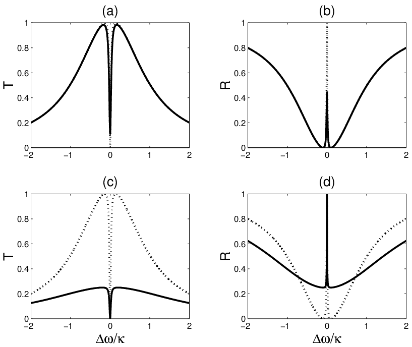
Let us stress that the reflection can be total even if the cavity is leaky. This apparently striking result is due to a totally constructive interference between the driving field and the field radiated by the optical system, which cannot be split into a cavity and an atom, but must be considered as a whole. This feature also appears on the normalized leaks on resonance ${\cal L}$ given by $R+T=1-{\cal{L}}$ , which fulfills

{\cal L}=2\sqrt{R}\sqrt{T}=\frac{2Q}{Q_{0}}\frac{1}{1+f}\left(1-\frac{Q}{Q_{0}}\frac{1}{1+f}\right)

(43)

The leaks can be approximated for $f\gg 1$ by the following expression

{\cal L}\sim\frac{2Q}{Q_{0}f}=\frac{2\gamma_{at}}{\Gamma},

(44)

which has a clear physical meaning : the leaks can be interpreted as the rate of photons lost by the atom over the rate of photons funneled in the output mode. This quantity decreases down to $0$ when the atomic leaks become vanishingly small, even if the atom is placed in a leaky cavity.

IV.2 Non-linear regime

We consider now the case of a leaky optical system described by equations (34). We shall restrict ourselves to the resonant case and to the semi-classical hypothesis. For sake of simplicity we shall also take $\gamma^{*}=0$ , which is a realistic hypothesis as it will be shown in the next section. As before we can adiabatically eliminate the cavity from the equations. Using the same definitions for $\Gamma$ , $f$ , $Q$ and $Q_{0}$ , we establish the optical Bloch equations for the leaky system

\begin{array}[]{l}\dot{s}={\displaystyle-\frac{\Gamma}{2}\frac{Q}{Q_{0}}\left(1+\frac{1}{f}\right)s+\sqrt{\frac{\Gamma}{2}}\frac{Q}{Q_{0}}(-2s_{z})ib_{in}}\\ \dot{s}_{z}={\displaystyle-\Gamma\frac{Q}{Q_{0}}\left(1+\frac{1}{f}\right)\left(s_{z}+\frac{1}{2}\right)+\sqrt{\frac{\Gamma}{2}}\frac{Q}{Q_{0}}(ib_{in}s^{*}+cc)}\\ b_{t}={\displaystyle-b_{in}\frac{Q}{Q_{0}}-i\sqrt{\frac{\Gamma}{2}}\frac{Q}{Q_{0}}s}\\ b_{r}={\displaystyle b_{in}\left(1-\frac{Q}{Q_{0}}\right)-i\sqrt{\frac{\Gamma}{2}}\frac{Q}{Q_{0}}s}\;.\par\end{array}

(45)

At it is shown in appendix B, the stationary solutions can be written

\begin{array}[]{l}s_{z}={\displaystyle-\frac{1}{2}\frac{1}{1+x^{{}^{\prime}}}}\\ s={\displaystyle\sqrt{\frac{\Gamma}{2}}\frac{ib_{in}}{1+x^{{}^{\prime}}}\frac{1}{1+{\displaystyle\frac{1}{f}}}}\;.\end{array}

(46)

with modified values for the saturation parameter $x^{{}^{\prime}}$ and the critical power $P_{c}^{{}^{\prime}}$

\begin{array}[]{l}x^{{}^{\prime}}={\displaystyle|b_{in}|^{2}/P_{c}^{{}^{\prime}}}\\ P_{c}^{{}^{\prime}}={\displaystyle\frac{\Gamma}{4\beta^{2}}}\;.\\ \end{array}

(47)

We have introduced the parameter $\beta={\displaystyle\frac{f}{1+f}}$ . The quantity $\beta^{2}$ can be seen as the probability for a resonant photon sent in the input mode to be absorbed by the optical system. The power necessary to saturate the two-level system, that is to reach $s_{z}=-1/4$ , is higher than in the ideal case which is a natural consequence of the leaks. The transmission coefficient in energy can be written

T={\displaystyle\left(\frac{Q}{Q_{0}}\right)^{2}\left[\frac{\beta}{1+\beta^{2}x}-1\right]^{2}}\;.

(48)

We have plotted in figure 9 the transmission coefficient $T$ as a function of the saturation parameter in the non-leaky case $x=4P_{in}/\Gamma$ . The limit of the signal for $x\rightarrow 0$ is $T_{min}$ because the two-level system is not saturated. If $x\rightarrow\infty$ the signal tends to $T_{max}$ : when the two-level system is saturated, the optical system behaves like an empty cavity. On the left, we fixed $\beta=1$ which may be realized with high values of the ratio $f$ , and we considered different leaky cavities. In this case, the transmission coefficient simply corresponds to the ideal transmission coefficient multiplied by $(Q/Q_{0})^{2}$ . On the right, we have considered a non-leaky cavity ( $Q/Q_{0}=1$ ) and different values of the ratio $f$ . The jump happens for higher values of the saturation parameter, which was expected.

V Feasibility study

In the two previous sections, we have seen that a one-dimensional atom, even leaky, induces the reflection of a low intensity driving field, giving rise to a highly dispersive transmission pattern, and behaves like a giant non-linear medium, with typical switching intensities of one photon per lifetime. This section aims at showing that these striking features can be observed using solid state two-level systems and cavities. As a first step, we shall comment on the validity of the two-level system model in the case of a single exciton embedded in a quantum dot. As a second step, we will focus on a well-known semi-conducting microcavity whose caracteristics depend on a small set of easily adjustable parameters : the micropillar. Micropillars are very good candidates for this application because the light they emit is directional. As a consequence they have already been used with success as single photon sources Solomon; Moreau01 and indistinguishable photon sources Var05. We shall optimize these parameters in view of observing the dipole induced reflection or the non-linear effect. As a third step we will draw a comparison between the performances of the device when it is operated as a single photon source or as a giant non-linear medium.

V.1 How good a two-level system is a semiconductor quantum dot ?

Semiconductor quantum dots displaying a very high structural and optical quality can be obtained using self-assembly in molecular beam epitaxy jmg2. Such nanostructures confine both electrons and holes on the few-nanometer scale, and support therefore a discrete set of confined electronic states. In its ground state $\left|g\right\rangle$ , the quantum dot is empty, whereas the lowest bright energy level $\left|e\right\rangle$ corresponds to the situation where it contains one electron-hole pair called exciton. Sharp atomic like fluorescence marzin and absorption karrai lines, associated to optical transitions between $\left|e\right\rangle$ and $\left|g\right\rangle$ can be observed experimentally.

As far as the spin structure is concerned, the projection of the electronic spin on the growth axis of the dot is either $1/2$ or $-1/2$ , whereas the projection of the hole’s spin is either $3/2$ or $-3/2$ (”heavy holes”). This corresponds to four distinct spin values for the exciton. However, only two excitons are coupled to the ground state by the electromagnetic field, namely $\left|-1/2,3/2\right\rangle$ and $\left|1/2,-3/2\right\rangle$ (”bright” excitons). The two other excitons have a total spin projection of $2$ or $-2$ . They remain optically uncoupled or ”dark” because of the selection rules governing the dipolar electrical hamiltonian, and they don’t have to be taken into account.

For a quantum dot showing perfect cylindrical symmetry around its growth axis, the two excitonic states are degenerate. In practice the symmetry is not perfect and the exchange interaction splits the doublet in two eigenstates, which are coupled to the ground state by two orthogonally linearly polarized fields bayer. At this point, a quantum dot appears as a ”V-type” system rather than as a two-level system. However, recent experiments have shown that in a cryogenic environment and under resonant pumping, which will correspond to our experimental conditions, electrons’ and holes’ spins are frozen at the exciton lifetime scale paillard. As a consequence, it is possible to work at a given linear polarisation and to ignore the other excitonic spin state, allowing an effective treatment of the quantum dot as a two-level system.

One could fear that pumping the quantum dot beyond its saturation intensity may lead to the creation of two electron-hole pairs (biexcitonic states, denoted XX). However, because of the interaction between two excitons, the transition between XX and $\left|e\right\rangle$ is energetically different (a few meV typically) from the transition between $\left|e\right\rangle$ and the fundamental state $\left|g\right\rangle$ . This effect allows to address spectrally the excitonic state under interest : if the driving field is resonant with the excitonic transition (which is the case in the demonstration of the giant non-linearity) or slightly detuned from the excitonic transition (which is the case in the experiments aiming at showing the dipole induced reflection, where the detuning is less than $1$ meV, corresponding to the spectral width of a micropillar), XX does not have to be taken into account.

The interaction of the exciton with the phonons of the surrounding matrix is responsible for a dephasing time of the excitonic dipole which may be much faster than the radiative recombination of the exciton kammerer02. Furthermore, fluctuating charges in the quantum dot environment can also induce significant dephasing under non-resonant optical excitation berthelot. We have taken this effect into account by introducing the parameter $\gamma^{*}$ in equations (34) and we have shown that it could lead to a drastic reduction of the contrast of the dipole induced reflection signal. However, excitonic dephasing times limited by radiative recombination have already been observed for a resonant excitation of the fundamental optical transition of InAs quantum dots at low temperature langbein04. Experiments aiming at the demonstration of the giant non-linearity will in fact be performed under similar conditions. This justifies taking $\gamma^{*}=0$ in the non-linear study including leaks.

To conclude this part, let us stress the fact that quantum Rabi oscillations rabi have been observed by resonantly pumping a single quantum dot of InAs at low temperature. This observation, as well as the successful demonstration of the coherent control of the excitonic transition controlecoh, show that quantum dots can be considered as two-level systems and used to realize atomic-physics like experiments, provided these are properly implemented.

V.2 Optimization of the cavity

We aim at optimizing the parameters of a micropillar in order to have a maximally contrasted signal. We can experimentally control two parameters: the intrinsic quality factor $Q_{0}$ and the diameter $d$ of the micropillar. $Q_{0}$ corresponds to the quality factor of the planar cavity and is tunable by changing the reflectivity of each Bragg mirror. The diameter $d$ is adjusted during the lithography and etching step. The total quality factor $Q$ of the micropillar reads

\frac{1}{Q}=\frac{1}{Q_{0}}+\frac{1}{Q_{leak}}\;,

(49)

where the leaks are mainly due to the etching step and can be written rivera99

\frac{1}{Q_{leak}}=\frac{2|E(d)|^{2}\varepsilon}{d}.

(50)

$|E(d)|$ is the electrical field of the fundamental mode at the sidewalls of the micropillar, whose profile is given by the Bessel function of the first kind $J_{0}$ rivera99. The parameter $\varepsilon$ is a parameter quantifying the etching quality. The leaks increase as the diameter of the etched micropillar decrases. In the following we will take $\varepsilon\sim 0.007$ which corresponds to realistic experimental parameters jmg.

The experimental signal to maximize is defined as ${\cal C}=T_{max}-T_{min}$ , where $T_{max}$ and $T_{min}$ are given by equations (41) and (42), $T_{max}=(Q/Q_{0})^{2}$ and $T_{min}=(Q/Q_{0})^{2}(1/(1+f))^{2}$ . We have chosen to optimize an amplitude rather than a visibility ${\cal V}=(T_{max}-T_{min})/(T_{max}+T_{min})$ because we should be then less sensitive to the optical background. A first strategy to optimize the contrast ${\cal C}$ is to reach small $T_{min}$ , that is high Purcell factor $F_{p}$ , whose expression is gerard99

F_{p}=\frac{3Q}{4\pi^{2}V}\left(\frac{\lambda}{n}\right)^{3}\;.

(51)

The quantity $\lambda$ is the dipole wavelength in the vacuum, $n$ the refractive index of the medium and $V$ the effective volume of the mode,

V\sim\left(\frac{\lambda}{n}\right)\frac{\pi d^{2}}{8}.

(52)

Figure 10 represents the evolution of $Q$ and $F_{p}$ as functions of the micropillar diameter for three different values of the intrinsic quality factor $Q_{0}$ : $1000,5300$ and $10000$ . If the diameter is too small, the leaks degrade $Q$ and as a consequence $F_{p}$ . If the diameter is too large, $F_{p}$ decreases because of the large modal volume. The diameters maximizing the Purcell factor vary between $1$ and $2$ $\mu m$ . As it can be seen on the figure, a higher initial $Q_{0}$ allows to reach higher values of $F_{p}$ , and corresponds to higher optimal diameters.

At the same time we need high $T_{max}$ , which corresponds to small cavity leaks and to large diameters. We have represented in figure 11 the evolution of $T_{max}-T_{min}$ as a function of the micropillar diameter for different $Q_{0}$ . As expected, the optimal diameters are higher than the ones obtained by optimization of Purcell factor, and vary now between $2$ and $6$ $\mu m$ . For each $Q_{0}$ , the amplitude of the optimized signal is higher than $0.8$ which is quite convenient. We shall prefer the set of parameters corresponding to the smallest diameter, so that it is easier to isolate a single quantum dot, that is $Q_{0}=1000$ , $d=2.4$ $\mu m$ , $Q=960$ and $F_{p}=2.6$ . The expected amplitude of the experimental signal should then be $0.85$ .

We shall mention here another strategy to enhance $f$ , that consists in reducing the leaks $\gamma_{at}$ . Recent experiments involving the metallization of the micropillars have shown a reduction of $\gamma_{at}$ by a factor 10 bayer01. The expected $T_{min}$ obtained with such a metallized cavity should be under $10^{-3}$ , and the signal amplitude near $0.9$ .

To have a glimpse of the expected signal we have plotted in figure 12 the transmission of the system as a function of the detuning between the atom and the field for $Q_{0}=1000$ , $Q=500$ and $F_{p}=3$ (dot curve) which corresponds to realistic parameters for single photon sources before optimization Moreau01. The contrast of the signal is $0.21$ . On the same figure we have also plotted the expected signal after optimization of the micropillar, with and without metallization of its sidewalls.

We have finally plotted in figure 13 the transmission coefficient on resonance as a function of the logarithm of the saturation parameter $\log(x)$ for these three different sets of parameters. We shall be able to observe the non-linear transmission jump with state-of-the-art micropillar cavities.

V.3 Single-photon source versus giant non-linear medium

We have seen that the ”one-dimensional atom” case requires $f\rightarrow\infty$ and $Q/Q_{0}\rightarrow 1$ . Such an optical system would also provide a high efficiency single-photon source. The expression of the raw quantum efficiency $\eta$ barnes of theses devices is indeed

\eta=\frac{f}{1+f}\frac{Q}{Q_{0}}\;.

(53)

The prefactor $\beta=f/(1+f)$ has been introduced in section IV, it represents the fraction of photons spontaneously emitted by the excited atom into the cavity mode, whereas $Q/Q_{0}$ is the fraction of photons initially in the cavity mode finally funneled into the mode(s) of interest. Note that usually for single-photon sources, the photons are collected in only one output mode. In the present case, transmitted and reflected photons must be collected to measure the quantum efficiency of the corresponding source. One may ask if optimizing the system as a single photon source is equivalent to optimizing it as a medium providing dipole induced transparency (one should then maximize the visibility ${\cal C}$ of the signal) or as a giant non-linear medium (this would require a low critical power, that is a high absorption probability $\beta^{2}$ as it has been introduced in section IV). We have plotted in figure 14 the parameters ${\cal C}$ , $\beta^{2}$ and $\eta$ as functions of the diameter of the micropillar for an initial quality factor $Q_{0}=1000$ . As it can be seen on the figure, optimal diameters are different. The optimization of ${\cal C}$ leads to the highest diameter. As it is explained in paragraph B, this is because non-leaky cavities (and as a consequence high diameters) are needed to reach high $T_{max}$ . It is striking to observe that $\beta^{2}$ and $\eta$ have different evolutions. Indeed one could have thought that a good single-photon source, that is an optical system that emits photons with high efficiency in a particular mode, is also able, when it is driven by a resonant field, to absorb and reemit photons with high efficiency. Yet $\beta^{2}$ is optimized for smaller diameters that $\eta$ : the absorption probability is more sensitive to the atomic leaks than the single photon source efficiency. Even if the cavity is leaky, an atom perfectly connected to the cavity mode can absorb one photon in the input field with a maximal probability. The major difference between these two behaviors is that they are observed in two quite different regimes. The quantity $\eta$ is the probability of detecting a photon in the mode of interest conditioned on the excitation of the atom, and can be computed by supposing that in a first step, the atom has emitted a photon in the cavity mode, and that in a second step, this photon has been funneled into the mode of interest. On the contrary, $\beta^{2}$ is estimated in a permanent regime where the driving field can interfere with the fluorescence field as it was pointed out in section III. A signature of this effect has been observed in section IV, where total reflection was induced by an atom perfectly connected to a leaky cavity. Because of this interference phenomenon, it is impossible to describe the evolution of the photon by successive interactions with the cavity mode and with the atom : the atom-cavity coupled system must be considered as a whole.

VI Perspectives

There has been a considerable number of proposals, e.g. cirac; pellizzari; duan, and experiments, e.g. rausch; kuhn, concerning the use of single emitters in high-finesse cavities for quantum information processing. Most of these papers are based on achieving the strong coupling regime. A recent proposal relying on the Purcell regime waksprl requires the coherent control of additional levels in the emitter. It is natural to ask whether the most basic non-linearity considered in the present paper could be used directly for quantum information applications, for example for implementing a controlled phase gate between two photons, as suggested in Refs. turchette95A; hofmann03. Unfortunately recent results suggest that this may not be possible. A numerical study kojima04 found fidelities of quantum gates employing the present non-linearity of order 80 %, which is quite far from what would be desirable for quantum computing or even quantum communication. Higher fidelities are elusive because the interaction with the single two-level system introduces temporal correlations between the two input photons. An analogous difficulty is discussed in detail in a recent theoretical paper on the use of Kerr non-linearities for quantum computing shapiro. From a quantum information perspective the relatively simple situation considered in the present paper may thus best be seen as an important step towards the realization of more complex configurations.

Another perspective opened by the implementation of this device concerns the photonic computation at low threshold. As it is shown in appendices D and E, the non-linearity studied in this paper is not intense enough to provide bistability, but could be used to reshape low intensity signals which may propagate in a photonic computer. The expected performances of the device are orders of magnitude higher than for usual saturable absorbers. Besides, if it is fed with single photons rather than with classical fields, this device could be operated as an all-optical switch at the single photon level, which is a fundamental component of a photonic computer. The theory developed in the frame of this paper could be adapted to model such a gate and optimize its performances. This work is under progress.

VII Conclusion

We have shown that a single two-level system in Purcell regime is a medium with appealing non-linear optical properties. In the linear case the two-level system prevents light from entering the cavity : this is dipole induced reflectance. This property vanishes as soon as the two-level system is saturated, which happens for very low power, of the order of one photon per lifetime (typically $1$ nW). As a consequence, such a medium shows a sensitivity at the single-photon level. We have established the optical Bloch equations describing this behavior in the semi-classical context, and shown that signatures of the non-linearity should be observable using quantum dots and state-of-the-art semiconducting micropillars as two-level systems and cavities respectively. We have explored possible applications of the non-linearity in the context of photonic information processing.

VIII Acknowledgments

This work is supported by the Agence Nationale de la Recherche under the project IQ-Nona. Alexia Auffeves-Garnier is very grateful to Xavier Letartre for the numerous and fruitful conversations. Christoph Simon thanks Nicolas Gisin for the final reference.

Appendix A Derivation of equation (14)

We show in this section that $(b_{r},b_{t})$ and $(b_{in},b_{in}^{{}^{\prime}})$ are related by a unitary transformation. For sake of completeness we keep the general form for $\theta_{1}$ and $\theta_{2}$ . Equations (13) can be written in the stationary linear case

S_{-}=\sqrt{\frac{2}{\Gamma}}\frac{ib_{in}+ib_{in}^{{}^{\prime}}}{1+{\displaystyle\frac{2i\Delta\omega}{\Gamma t_{0}(\Delta\omega)}}}\;.

(54)

As a consequence, $b_{t}$ reads

b_{t}=t_{0}(\Delta\omega)\left(-1+\frac{1}{1+{\displaystyle\frac{2i\Delta\omega}{\Gamma t_{0}(\Delta\omega)}}}\right)b_{in}+\left(1-t_{0}(\Delta\omega)+\frac{t_{0}(\Delta\omega)}{1+{\displaystyle\frac{2i\Delta\omega}{\Gamma t_{0}(\Delta\omega)}}}\right)b_{in}^{{}^{\prime}}\;.

(55)

It can be rewritten in the following way

b_{t}=-\frac{1}{1+i\zeta}b_{in}+\frac{i\zeta}{1+i\zeta}b_{in}^{{}^{\prime}}\;,

(56)

with

\zeta=\frac{\Delta\omega+\delta}{\kappa}-\frac{\Gamma}{2\Delta\omega}\;.

(57)

We easily compute $b_{r}$ by switching $b_{in}$ and $b_{in}^{{}^{\prime}}$ . We finally obtain

\left(\begin{array}[]{c}b_{r}\\ b_{t}\end{array}\right)=\left(\begin{array}[]{c c}{\displaystyle\frac{i\zeta}{1+i\zeta}}&{\displaystyle\frac{-1}{1+i\zeta}}\\ {\displaystyle\frac{-1}{1+i\zeta}}&{\displaystyle\frac{i\zeta}{1+i\zeta}}\end{array}\right)\left(\begin{array}[]{c}b_{in}\\ b_{in}^{{}^{\prime}}\end{array}\right)\;.

(58)

The scattering matrix can be written in the following form

S=\frac{e^{i\phi}}{{\sqrt{1+\zeta^{2}}}}\left(\begin{array}[]{c c}\zeta&i\\ i&\zeta\end{array}\right)\;,

(59)

with

\phi=\arctan\left(\frac{1}{\zeta}\right)\;.

(60)

The $S$ matrix is a unitary transformation up to a global phase. As a consequence energy is conserved by this transformation. Keeping in mind this property we shall rather use the form (58) whose coefficients have a more direct physical interpretation.

Appendix B Derivation of the critical intensity including leaks

In this section we derive the expression for the critical intensity in the non-resonant case in presence of leaks. We use the notations introduced in section IV. To recover the results exploited in section III we shall impose $Q=Q_{0}$ and $1/f\rightarrow 0$ . As it is justified in section V, we suppose $\gamma^{*}=0$ . The stationary cavity population writes

a={\displaystyle t^{{}^{\prime}}_{0}\frac{Q}{Q_{0}}\frac{-\Omega S_{-}+\sqrt{\kappa}(ib_{in}+b_{in}^{{}^{\prime}})+H}{\kappa}}\;,

(61)

where $t^{{}^{\prime}}_{0}$ has the following expression

t^{{}^{\prime}}_{0}=\frac{1}{{\displaystyle 1+i\frac{Q}{Q_{0}}\frac{\Delta\omega+\delta}{\kappa}}}\;.

(62)

The semi-classical equations describing the evolution of $s_{z}$ and $s$ write

\begin{array}[]{l}\dot{s}=-i\Delta\omega s-{\displaystyle\frac{\Gamma}{2}\frac{Q}{Q_{0}}\left[t^{{}^{\prime}}_{0}+\frac{1}{f}\right]s-i\frac{Q}{Q_{0}}\sqrt{\frac{\Gamma}{2}}(2s_{z})b_{in}t^{{}^{\prime}}_{0}}\\ \dot{s}_{z}={\displaystyle-\Gamma\frac{Q}{Q_{0}}\left[\Re\left(t^{{}^{\prime}}_{0}\right)+\frac{1}{f}\right]\left(s_{z}+\frac{1}{2}\right)+\sqrt{\frac{\Gamma}{2}}\frac{Q}{Q_{0}}\left[is^{*}b_{in}t^{{}^{\prime}}_{0}+cc\right]}\;.\end{array}

(63)

where $f$ , $Q$ and $Q_{0}$ have been defined in section III. By sake of completeness we also give the expressions for $b_{t}$ and $b_{r}$ after adiabatic elimination of the cavity mode

\begin{array}[]{l}b_{t}={\displaystyle-\frac{Q}{Q_{0}}t^{{}^{\prime}}_{0}b_{in}-i\frac{Q}{Q_{0}}\sqrt{\frac{\Gamma}{2}}t^{{}^{\prime}}_{0}s}\\ b_{r}={\displaystyle(1-\frac{Q}{Q_{0}}t^{{}^{\prime}}_{0})b_{in}-i\frac{Q}{Q_{0}}\sqrt{\frac{\Gamma}{2}}t^{{}^{\prime}}_{0}s}\;.\end{array}

(64)

We obtain the stationary solution for $s$

s=-{\displaystyle i\sqrt{\frac{2}{\Gamma}}\frac{2s_{z}b_{in}t^{{}^{\prime}}_{0}}{{\displaystyle t^{{}^{\prime}}_{0}+\frac{1}{f}+\frac{2i\Delta\omega}{\Gamma}\frac{Q_{0}}{Q}}}}\;.

(65)

Injecting this solution in the evolution equation for $s_{z}$ , we find

\dot{s}_{z}=0={\displaystyle\frac{1}{2}+s_{z}\left(1+\frac{|b_{in}|^{2}}{P_{c}^{{}^{\prime}}}\right)}\;,

(66)

with

\frac{1}{P_{c}^{{}^{\prime}}}=\frac{2|t^{{}^{\prime}}_{0}|^{2}}{\Gamma(\Re(t^{{}^{\prime}}_{0})+1/f)}\left(\frac{1}{1/f+2i\frac{Q_{0}}{Q}\frac{\Delta\omega}{\Gamma}+t_{0}^{{}^{\prime}}}+cc\right)\;.

(67)

Noting that $2\Re(t^{{}^{\prime}}_{0})+1/f=2/f-t^{{}^{\prime}}_{0}-{t^{{}^{\prime}}_{0}}^{*}$ we have

P_{c}^{{}^{\prime}}=\frac{\Gamma}{4|t^{{}^{\prime}}_{0}|^{2}}\left(\frac{1}{f^{2}}+\frac{1}{{f}}(t^{{}^{\prime}}_{0}+{t^{{}^{\prime}}_{0}}^{*})+\frac{2i\Delta\omega}{\Gamma}\frac{Q_{0}}{Q}(-t^{{}^{\prime}}_{0}+{t^{{}^{\prime}}_{0}}^{*})+\left(\frac{Q_{0}}{Q}\frac{2\Delta\omega}{\Gamma}\right)^{2}+|t^{{}^{\prime}}_{0}|^{2}\right)

(68)

Let us remind here of the following expressions

\begin{array}[]{l}{\displaystyle\frac{1}{|t^{{}^{\prime}}_{0}|^{2}}=\left(\frac{Q}{Q_{0}}\right)^{2}+\left(\frac{\Delta\omega+\delta}{\kappa}\right)^{2}}\\ {\displaystyle\frac{t^{{}^{\prime}}_{0}+{t^{{}^{\prime}}_{0}}^{*}}{|t^{{}^{\prime}}_{0}|^{2}}=2}\\ {\displaystyle\frac{-t^{{}^{\prime}}_{0}+{t^{{}^{\prime}}_{0}}^{*}}{|t^{{}^{\prime}}_{0}|^{2}}=\frac{2iQ}{Q_{0}}\frac{\Delta\omega+\delta}{\kappa}}\end{array}

(69)

We finally obtain

P_{c}^{{}^{\prime}}=\frac{\Gamma}{4}\phi^{{}^{\prime}}(\Delta\omega)\;,

(70)

with

\phi^{{}^{\prime}}(\omega)={\displaystyle\left(1+\frac{1}{f}\right)^{2}+\left(\frac{Q}{Q_{0}f}\frac{\Delta\omega+\delta}{\kappa}\right)^{2}+\left(\frac{2\Delta\omega}{\Gamma}\frac{Q_{0}}{Q}\right)^{2}+\left(\frac{2\Delta\omega}{\Gamma}\frac{\Delta\omega+\delta}{\kappa}\right)^{2}-\left(\frac{4\Delta\omega}{\Gamma}\frac{\Delta\omega+\delta}{\kappa}\right)}\;.

(71)

If the system has no leaks, we have

\phi^{{}^{\prime}}(\Delta\omega)=\phi(\Delta\omega)=\left(\frac{2\Delta\omega}{\Gamma}\right)^{2}+\left(\frac{2\Delta\omega}{\Gamma}\frac{\Delta\omega+\delta}{\kappa}-1\right)^{2}

(72)

Whatever the driving frequency may be, the absorption cross section remains positive. This expression in mainly used in section III. At resonance, we find

\phi^{{}^{\prime}}(0)=\frac{1}{\xi}={\displaystyle\left(1+\frac{1}{f}\right)^{2}}\;,

(73)

which was also exploited in section III.

Appendix C Slow light

We have evidenced in section III and IV that a one-dimensional atom is a highly dispersive medium. In particular, a quantum-dot cavity system evanescently coupled to a waveguide has a behavior similar to a medium showing dipole induced transparency. As a consequence, this optical system could be used to slow down photons. Let us consider the case of a cavity perfectly connected to a waveguide ( $Q/Q_{0}=1$ ) containing a leaky quantum dot. The transmission coefficient in amplitude can be written $t=|t|e^{-i\phi_{t}(\omega)}$ , where $\phi_{t}(\Delta\omega)$ varies near $\omega_{0}$ on a scale $\Gamma$ . We send in the optical system a wave packet $\psi_{in}(\omega)$ of width $W$ centered around $\omega_{0}$ . Denoting $\theta$ the temporal coordinate, we obtain the shape of the output pulse

\psi_{out}(\theta)\propto\int d\omega\psi_{in}(\omega)e^{i\omega\theta}e^{i\phi_{t}(\omega)}\;.

(74)

If the width of the wave packet fulfills $W\ll\Gamma$ , we can develop $\phi_{t}$ around $\omega_{0}$ . We finally obtain $\psi_{out}(\theta)=\psi_{in}\left[\theta-{\displaystyle\left(\frac{\partial\phi_{t}}{\partial\omega}\right)_{\omega_{0}}}\right]$ . The wave packet will then be transmitted by the optical system after a delay $T_{D}$ which reads

T_{D}=\left(\frac{\partial\phi_{t}}{\partial\omega}\right)_{\omega_{0}}\;.

(75)

During the transmission the wave packet will also be damped by a factor $T=|t|^{2}$ . Remembering that $\kappa\gg\Gamma$ , we neglect the variations due to the cavity mode. We shall then take $t^{{}^{\prime}}_{0}(\Delta\omega)\sim 1$ and

t\sim\frac{f}{1+f}\frac{1}{{\displaystyle 1+\frac{2i}{\Gamma}\Delta\omega\frac{Q}{Q_{0}}\frac{f}{1+f}}}\;.

(76)

With this hypothesis, $\phi_{t}\sim\arctan\left(\frac{f}{1+f}\frac{2\Delta\omega}{\Gamma}\right)$ . As a consequence,

T_{D}\sim\frac{2}{\Gamma}\arctan^{{}^{\prime}}(x)_{0}\sim\frac{2}{\Gamma}\frac{f}{1+f}\;.

(77)

The wave packet is delayed by the lifetime of the dipole, which was expected. The damping factor has the following form

T=\left(\frac{f}{1+f}\right)^{2}

(78)

This process could be repeated using a series of $N$ optical devices. We note $N_{1/2}$ the number of devices such that the outcoming power is half the incoming one. $N_{1/2}$ checks

N_{1/2}=\frac{1}{2}\frac{\log{2}}{\log(1+1/f)}

(79)

Supposing $f$ sufficiently high, we have $\log(1+1/f)\sim 1/f$ and $N_{1/2}$ scales like $f$ . We could finally obtain a delay ${\cal T}_{D}$

{\cal T}_{D}=N_{1/2}\frac{2}{\Gamma}\frac{f}{1+f}\propto\frac{\Gamma}{2}f

(80)

In particular, we could use a series of microdisks each evanescently coupled to the same wave guide. This generalizes the study of Heebner et al Heebner02 who have shown that the group velocity of a signal passing through a series of empty microdisks scales like the inverse of the finesse of the resonators.

Appendix D About optical switches

Looking at the transmission coefficient, we could be tempted to use the giant non-linearity to realize an all-optical switch. Bistability regime is expected to be quite useful with this aim notomi05; tanabe05. As it is represented on figure 15, we could for example re-inject part of the transmitted intensity in the input port to realize a bistable device. Unfortunately the slope of the signal is too low. Calling $P_{0}$ the signal coming in the loop, $P_{e}$ the signal entering the device, $P_{t}$ the power transmitted by the device and $A$ the fraction of $P_{t}$ used to create the bistability, we have

P_{e}=P_{0}+AP_{t}(P_{e})\;.

(81)

Bistability happens for values of the parameter $B$ for which equation $P_{0}(P_{e})=B$ has more than one solution. At low intensity $P_{t}\sim 0$ and $P_{e}\sim P_{0}$ . At high intensity $P_{t}\sim P_{0}$ and $P_{e}\sim(1-A)P_{0}$ . The system will exhibit bistability if $P_{0}$ decreases as $P_{e}$ increases. This can only be done if $\partial P_{t}/\partial P_{e}>1$ . Nevertheless, in can easily be shown that the slope of the signal $P_{t}(P_{e})$ is bounded by $(2/3)^{3}<1$ , preventing the system from reaching the bistability regime.

Appendix E Reshaping step

A possible application is to use the non-linearity to enhance the contrast ratio between two pulses of different intensities. This can be used to regenerate optical signals travelling in an optical fiber. The major advantage of this system compared to other devices is the very low switching energy, defined as the energy necessary to saturate the system and make it switch from a linear to a non-linear behavior. As already seen, the typical switching energy is $0.25$ $h\nu$ where $h\nu$ the energy of a resonant photon. We have $h\nu\sim 1~eV\sim 4.10^{-20}J$ which is $8$ orders of magnitude lower than for traditional saturable absorbers oudar. The figure of merit for this kind of devices is the contrast enhancement ratio, defined as

{\cal C}=\left(\frac{P_{L}}{P_{H}}\right)_{in}\left(\frac{P_{H}}{P_{L}}\right)_{t}

(82)

where $P_{H}$ (resp $P_{L}$ ) is the high-power pulse (resp the low one). The subscript _in (resp _t) describes the incoming field (resp transmitted). We introduce the extinction ration of the pulse

d=\left(\frac{P_{H}}{P_{L}}\right)_{in}\;.

(83)

For a perfect non-linear device, ${\cal C}$ writes

{\cal C}=\frac{1}{d}\frac{T(x)}{T(x/d)}\;,

(84)

where $T$ is the transmittance at resonance of the device. We have

{\cal C}=d\left(\frac{1+x}{1+x/d}\right)^{2}\;,

(85)

where ${\cal C}$ is maximum for $x\rightarrow 0$ and tends to $d$ . With an ideal device we could theoretically reach any value of ${\cal C}$ . Taking into account the leaks, and denoting $T_{leak}$ the transmission of the device on resonance, and ${\cal C}_{leak}$ the new contrast enhancement factor, we obtain

{\cal C}_{leak}=\frac{1}{d}\frac{T_{leak}(x)}{T_{leak}(x/d)}\;.

(86)

We have represented figure 16 the contrast enhancement factor for different values of the factor $f$ which has been defined in equation (39). Let us recall that $f$ is related to the Purcell factor by the simple expression $f=(\gamma_{free}/\gamma_{at})F_{p}$ if there is no excitonic dephasing. The intrinsic quality factor (resp. the quality factor) of the cavity has been taken equal to $1000$ (resp. $950$ ). The extinction ratio is doubled for $f\sim 30$ , which corresponds to a typical Purcell factor of $3$ , and $\gamma_{at}/\gamma_{free}\sim 0.1$ which could be obtained by metallizing the sidewalls of a micropillar cavity as it has been underlined in section V. The ratio increases with $f$ , a $6~dB$ enhancement is reached for $f\sim 100$ which is within reach of the micropillar or photonic crystal technology.

References

(1) R.J. Thompson, G. Rempe and H.J. Kimble, Phys. Rev. Lett. 68, 1132 (1992).
(2) M. Brune et al., Phys. Rev. Lett. 76, 1800 (1996).
(3) K.M. Birnbaum et al., Nature, 436, 87 (2005).
(4) T.H. Stievater et al., Phys. Rev. Lett. 87, 133603 (2001); H. Kamada, H. Gotoh,J. Temmyo,T. Takagahara, H. Ando, Phys. Rev. Lett. 87, 246401 (2001).
(5) T. Flissikowski, A. Betke, I. A. Akimov and F. Henneberger, Phys. Rev. Lett. 92, 227401 (2004); Q.Q. Wang et al., Phys. Rev. Lett. 95, 187404 (2005).
(6) J.P. Reithmaier et al., Nature 432, 197 (2004); T. Yoshie et al., Nature 432, 200 (2004); E. Peter et al., Phys. Rev. Lett. 95, 067401 (2005).
(7) E. M. Purcell, Phys. Rev. 69, 681 (1946).
(8) J. M. Gerard et al., Phys. Rev. Lett. 81, 1110 (1998)
(9) G.S. Solomon, M. Pelton and Y. Yamamoto, Phys. Rev. Lett. 86, 3903 (2001).
(10) E. Moreau et al., Applied Physics Letters 79, 2865 (2001).
(11) C. Santori et al., Nature 419, 594 (2002); S. Varoutsis et al., Phys. Rev. B. 72, 041303(R) (2005).
(12) Q.A. Turchette, C.J. Hood, W. Lange, H. Mabuchi and H.J. Kimble, Phys. Rev. Lett. 75, 4710 (1995).
(13) E. Waks and J. Vuckovic, Phys. Rev. A 73, 041803(R) (2006).
(14) E. Waks and J. Vuckovic Phys. Rev. Lett. 96, 153601 (2006).
(15) H.F. Hofmann, K. Kojima, S. Takeuchi and K. Sasaki, Journal of Optics B, 5, 218 (2003).
(16) Q. A. Turchette, R. J. Thompson and H. J. Kimble, Applied Physics B 60, S1-S10 (1995).
(17) C. W. Gardiner and M. J. Collett, Phys. Rev. A, 31, 3761 (1985).
(18) Y. Akahane et al, Optics Express 13, 2512 (2005).
(19) J. T. Shen and S. Fan, Optics Letters 30, 2001 (2005).
(20) K. Kojima, H.F. Hofmann, S. Takeuchi and K. Sasaki, Phys. Rev. A 70, 013810 (2004).
(21) Allen and Eberly, Optical resonance and two-level systems, Dover.
(22) J.E. Heebner, R.W. Boyd, Q-Han Park, Phys. Rev. E. 65, 036619 (2002).
(23) A. Kuhn, M. Hennrich and G. Rempe, Phys. Rev. Lett. 89, 067901 (2002).
(24) C. Cohen-Tannoudji et al., Processus d’interaction entre Photons et Atomes, Ed. CNRS, p.366.
(25) A. A. Said et al., J. Opt. Soc. Am. B 9, 405 (1992).
(26) J.P. Poizat and P. Grangier, Phys. Rev. Lett. 70, 271 (1993); J.F. Roch et al, Phys. Rev. Lett. 78, 634 (1997); P. Grangier et al, Nature 396, 537 (1998).
(27) L. V. Hau, S. E. Harris, Z. Dutton and C. W. Behroozi, Nature 397, 594 (1999).
(28) T. Rivera et al., Applied Physics Letters 74, 911 (1999).
(29) J. M. Gerard, Topics of Applied Physics 30, 269 (2003).
(30) J. M. Gerard et al., J. Cryst. Growth 150, 351 (1995).
(31) J.Y. Marzin, J.M. Gerard, A. Izrael, D. Barrier,G. Bastard, Phys. Rev. Lett. 73, 716 (1994).
(32) S. Seidl et al., Phys. Rev. B 72, 195339 (2005).
(33) M. Bayer et al., Phys. Rev. B 65, 195315 (2002).
(34) M. Paillard et al., Phys. Rev. Lett. 86, 1634 (2000).
(35) C. Kammerer et al., Phys. Rev. B 66, 041306(R) (2002).
(36) A. Berthelot et al., Nature Physics 2, 759 (2006).
(37) W. Langbein et al., Phys. Rev. B 70, 033301 (2004).
(38) M. Bayer et al., Phys. Rev. Lett. 86, 3168 (2001).
(39) W. L. Barnes et al., Eur. Phys. J. D 18, 197 (2002).
(40) M. Notomi et al., Optics Express 13, 2678 (2005);
(41) T. Tanabe et al. , Optics Letters 30, 2575 (2005);
(42) J. Mangeney et al., Electronic Letters 36, 1486 (2000).
(43) J.I. Cirac, P. Zoller, H. J. Kimble and H. Mabuchi, Phys. Rev. Lett. 78, 3221 (1997).
(44) T. Pellizzari, S. A. Gardiner, J. I. Cirac and P. Zoller, Phys. Rev. Lett. 75, 3788 (1995).
(45) L.-M. Duan and H. J. Kimble, Phys. Rev. Lett. 92, 127902 (2004).
(46) A. Rauschenbeutel et al., Phys. Rev. Lett. 83, 5166 (1999).
(47) J.H. Shapiro, Phys. Rev. A 73, 062305 (2006).