Conditional control of the quantum states of remote atomic memories
for quantum networking
Quantum networks hold the promise for revolutionary advances in information processing with quantum resources distributed over remote locations via quantum-repeater architectures. Quantum networks are composed of nodes for storing and processing quantum states, and of channels for transmitting states between them. The scalability of such networks relies critically on the ability to perform conditional operations on states stored in separated quantum memories. Here we report the first implementation of such conditional control of two atomic memories, located in distinct apparatuses, which results in a 28-fold increase of the probability of simultaneously obtaining a pair of single photons, relative to the case without conditional control. As a first application, we demonstrate a high degree of indistinguishability for remotely generated single photons by the observation of destructive interference of their wavepackets. Our results demonstrate experimentally a basic principle for enabling scalable quantum networks, with applications as well to linear optics quantum computation.
In recent years, it has been established that quantum memory is an essential component for the distribution of entanglement over arbitrarily long distances using quantum repeaters zoller05; briegel98. In the quantum repeater protocol, entanglement is distributed by entanglement swapping through a chain of spatially-separated entangled pairs of particles. Without memory, all pairs need to be entangled at the same time for the entanglement distribution to succeed, an event whose probability decreases exponentially as the length of the chain increases. On the other hand, if it is possible to store the entanglement in spatially-separated quantum memories and if one has a trigger that unambiguously heralds the entanglement once it is achieved chou05, it is possible to build up the chain of entangled pairs by entangling different parts of the chain at different times. By conditioning the evolution of the whole system to the output of its different parts, an exponential enhancement is attained in the probability of success of the protocol, which leads, for example, to the possibility of scalable long-distance quantum communication duan01. Let us note also that Linear Optical Quantum Computing knill01; franson04; nielsen04 or quantum state engineering, with schemes working in an iterative manner fiurasek03, are both damped exponentially by low success probability due to the present lack of synchronized single photon sources. Real-time control for synchronization of many sources is then a promising way to boost the probability of simultaneous generation of many target quantum states, and thereby to enable the practical realization of elaborate procedures.
Since photons are the basic carriers of information over long distances, the necessity of using memory for communication implies the need to control the exchange of quantum information between matter (stationary qubits) and light (flying qubits). Great progress has been achieved recently in this direction for different systems that could work as single nodes of a distributed quantum network cirac97. For example, generation of photon pairs kuzmich03; balic05; thompson06, storage of single photons Eisaman05; Chaneliere05, and high-efficiency retrieval of stored single excitations laurat06 were implemented with atomic ensembles. Entanglement between atoms and spontaneously emitted light was demonstrated with both single trapped atoms blinov04; volz06 and atomic ensembles Matsukevich05; deRiedmatten06. Heralded entanglement between two cold atomic ensembles by means of a single stored excitation was demonstrated last year chou05, followed more recently by the achievement of probabilistic (a posteriori) entanglement between two excitations stored in different ensembles Matsukevich06. In the continuous variables regime, deterministic entanglement has been obtained between two vapor cells at room temperature julsgaard01.
A key point that has not been experimentally addressed up to now, however, is the extent to which these different systems and techniques enable scalable quantum networks. Only recently three groups reported the use of feedback to enhance the probability of generating a photon using a heralded single photon source with memory deRiedmatten06; Matsukevich06b; chen06. In the present work, we report the first implementation of real-time conditional control of two distant quantum memories. The memory nodes consist of ensembles of cold atoms that can each store a single collective excitation in a probabilistic, but heralded, way duan01. Since this excitation can be transferred with high efficiency to a light field in the single-photon regime laurat06, the system functions as a heralded single-photon source, ideal for applications to quantum repeaters. The conditional control allows us to store an excitation in one ensemble, while waiting for a trigger signal indicating the presence of an excitation in the other ensemble. Relative to operation without this conditional control, we attain a factor of 28 increase in the probability to generate simultaneously a single photon from each system. Further increase is currently limited by the finite coherence time of our memory felinto05; deRiedmatten06.
For applications in quantum repeaters, it is crucial that single photons emitted by two different ensembles are indistinguishable when combined at a beam splitter, since this is at the heart of the technique to achieve measurement-induced entanglement duan01; simon03; chou05 and entanglement swapping duan01 between remote atomic systems. As a first application of our control system, we perform a time-resolved two-photon interference measurement to quantify the indistinguishability of the generated single photons, obtained simultaneously from atomic excitations stored for different amounts of time. We combine the photons at a beam splitter and observe a nonclassical suppression in the rate of joint detections at its two output ports mandel-wolf95. This suppression is the result of a destructive two-photon interference, as first demonstrated in a parametric down conversion system by Hong, Ou, and Mandel hong87. More recently such suppression was observed for photons emitted successively by a single source santori02; legero04 or simultaneously by different sources, such as spatially separated down-converters deRiedmatten03 and trapped atoms beugnon06. Our results show a suppression of % for the probability of having two photons leave the beam splitter through different ports, from which we infer an overlap for the wavepackets of the two single photons.
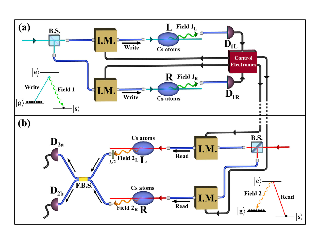
Our experimental setup is sketched in Fig. 1 (see also Methods section). The two ensembles consist of pencil-shaped clouds of cold cesium atoms located in two different vacuum chambers, 2.7 m apart. In the beginning of each trial, all atoms are optically pumped to the hyperfine ground state (see Fig. 1a). The atomic level structure for the writing process consists of the initial ground state ( level of atomic cesium), the ground state for storing a collective spin flip (), and the excited level (). Then a weak write pulse, lasting 38 ns, excites the transition. With a small probability , the atomic ensemble spontaneously emits a photon (field 1) on the transition, into the solid angle of our detection system. For our experimental conditions, the detection of this first photon heralds the storage of an excitation in a collective, symmetric mode of the whole ensemble duan01; laurat06; duan02.
This collective excitation can then be retrieved with high probability duan01; laurat06 by a strong read pulse (38 ns long and resonant to the transition) counterpropagating with respect to the write beam; see Fig. 1b. The read pulse results in the generation of a second photon (field 2) in the direction opposite to field 1 balic05. For both ensembles, a detection in field 1 occurs with probability and is followed by a detection in field 2 with conditional probability , which corresponds, after taking the losses in the field-2 channels into account, to retrieval efficiency for the collective mode at the output of the ensemble laurat06. If no detection in field 1 is registered in a given trial, the read pulse is fired in order to optically pump the atoms back to their initial condition. For the chosen , the normalized intensity cross-correlation function between fields 1 and 2 is measured to be approximately for both ensembles kuzmich03; laurat06, corresponding to a field 2 well within the single-photon regime, with a large suppression of its two-photon component laurat06. For our system, is already a strong indication of nonclassical correlations between fields 1 and 2 kuzmich03. The parameter quantifies this suppression by examining the probability of generating two photons in the same pulse, normalized by an equally bright Poisson-distributed source chou04. Classical fields must satisfy the Cauchy-Schwarz inequality ; for independent coherent states, , while for thermal fields, chou04. The parametric dependence of on for our system was investigated in detail in Refs. laurat06 and chou04, from which we infer for .
Fields , are guided to the respective detectors (,) (Fig. 1a). The field-2 outputs of the two ensembles, on the other hand, are combined at a fiber beam splitter, whose outputs are then directed to two detectors and (Fig. 1b). To exploit the quantum memory to speed up probabilistic quantum protocols that require concurrent state preparation in two atomic ensembles, we have designed and implemented a custom logic circuit that allows conditional control of the writing, storing, and reading operations for the atomic excitations. Upon receipt of a field-1 detection signal from one ensemble, the circuit gates off the write and read pulses for that ensemble, thereby storing a collective excitation in the atoms laurat06; deRiedmatten06; chou04. The write-read pulse train in the other ensemble is not affected. The storage stops and the excitations in the ensembles are read out when either of the following events occurs: (1) A field-1 photon is detected in the second system, prompting the circuit to release read pulses into the first and second ensembles, thereby simultaneously retrieving the stored excitations from both ensembles; (2) A pre-determined maximal storage time set in the circuit is reached in the first ensemble. Then, the storage ceases, and the ensembles are optically pumped back to the original condition. The logic circuit returns to its dormant state, passing all the write and read pulses to the ensembles, until the next field-1 detection signal triggers its function.

Our logic circuit is designed specifically to increase , the probability of having excitations stored simultaneously in each ensemble. Given an initial event in one ensemble, the filled squares in Fig. 2 show how increases as a function of the number of trials of duration ns that we wait for the other ensemble. The values in this curve were obtained by performing the experiment using a maximum number of trials (corresponding to our specific s), recording a file with the whole history of events, counting the number of events where the second ensemble was prepared up to trials after the first one, and then dividing this number by the total number of trials . After pulses, we observe an increase in , close to the expected value of for the case (see Methods Section). Note that for our experimental conditions, the conditional logic reduces (with reference to a try-until-success strategy) the number of trials in a negligible way, by up to (i.e., ). It is also important to point out that the advantage of such conditional logic will be (exponentially) more pronounced for larger systems involving more than two memories.
Our interest, however, is not directly in , but rather in the probability of obtaining joint detections for field 2 after the two systems have each stored a single excitation. In Fig. 2 (open circles) is given as a function of , for the case where the fields , from the two ensembles have orthogonal polarizations. Evidently, does not increase by the same factor as does , but grows instead only up to [i.e., times the value obtained without the control circuit ()]. This behavior is expected from the fact that the retrieval efficiency for the stored excitation in the ensemble that is first prepared decays until the other ensemble is prepared and the read pulses are fired. The coherence time for our system is about 10 s felinto05; deRiedmatten06, and can also be directly inferred from the decay with of the probabilities for one and two photo-detections in field 2 (see Appendix).
To characterize the indistinguishability of the photons in fields and , we perform a measurement of the suppression of joint-detection events at detectors in the same trial. In Fig. 3, we observe that the conditional joint-detection probability decreases for the situation where fields , are combined with the same polarizations (filled squares), compared to the case of orthogonal polarizations (open circles). The detection times are obtained from the record of events in our acquisition card, which has 2 ns resolution, much smaller than the duration of the photon wavepackets. From this list of detection times, we obtain the time difference between the two detections. To quantify the coincidence suppression shown in Fig. 3, we consider the visibility , where gives with orthogonal polarization and gives that with parallel polarization. Note that for ideal single photons with perfect overlap of their wavepackets, while for completely distinguishable fields. Obtaining and from the integration over of the respective data points in Fig. 3, we find (see also Appendix).

For photons orthogonally polarized, we fit our measurements for the joint-detection probability in Fig. 3 to a Gaussian (dashed line),
| (1) |
We find ns, from which the photon duration can be inferred assuming identical wavepackets. For perfectly transform-limited photons, the suppressed with parallel polarizations can be obtained from the one with perpendicular polarizations by multiplication by a constant scaling factor . When one introduces frequency jitter , can be expressed as legero04; beugnon06; legero03:
| (2) |
.
The green line gives such a fit with and . The jitter error bar is obtained by doubling the fitting parameter. This simple fit agrees well with the data and leads to a time-bandwidth product equal to , providing a good indication that our photons are close to transform limited. Others measurements are necessary to investigate this issue further.
The main cause of visibility reduction is that the two-photon components for the conditional fields , for both ensembles are necessarily nonzero laurat06. From the inferred value of two-photon suppression , we estimate with a simple model that the maximal achievable visibility for perfect overlap between the two fields is (see Appendix). By comparing our measured visibility to , we infer that the overlap of the field-2 wavepackets is , where for perfect mode-matching. The overlap mismatch can be partly explained by a non-zero polarization extinction ratio in the polarization-maintaining fibers (-14 dB). The visibility also decreases due to a small misalignment introduced by the rotation of the half-wave plate to switch between the two polarizations. The alignment was checked by analyzing the events where the two photons are created in different readout intervals, thus exhibiting no interference (see Appendix). In this case, the orthogonal-polarization joint-detection level is 0.08 smaller than for parallel polarization, which should increase the visibility by 0.02. Another small decrease in the visibility should come from the measured imbalance (0.51/0.49) of the fiber beam splitter. Note that the visibility of the two-photon interference can in principle be increased by reducing the intensity of the write pulses (and thereby and hence chou04; laurat06), but this comes at the expense of a reduced counting rate.
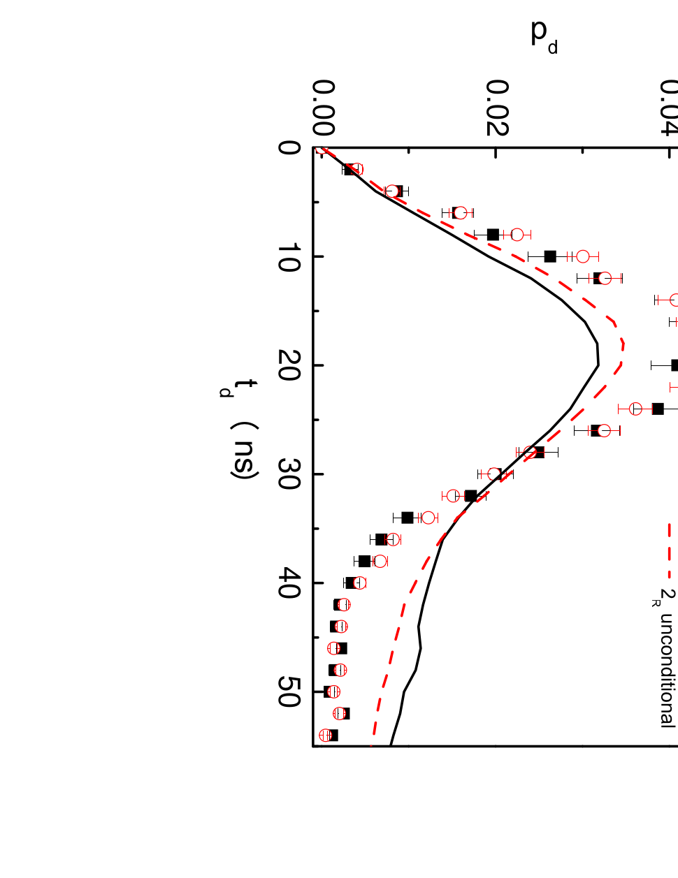
We also performed independent measurements to assess the temporal overlap of the two wavepackets. The temporal shape of the conditional wavepackets of fields , are given, respectively, by the filled squares and empty circles in Fig. 4. These wavepackets were obtained by blocking the fields from the other ensemble, disabling the logic circuit, and considering only the field 2 detections occuring in the same trial as a field 1 detection. The two wavepackets are quite similar, consistent with the good suppression we measured, and both have temporal widths around ns (Gaussian fit), which is also consistent with the expected width ns extracted from Fig. 3 by considering identical wavepackets. In Fig. 4 we also show the unconditional wavepackets for fields ,. They are considerably different from the conditional ones, indicating that part of the light we collect from the ensembles is not correlated to field 1, but likely arises from processes not related to the collective atomic state duan02.
In summary, we have demonstrated a -fold enhancement in the probability for simultaneous generation of single photons from two remote atomic ensembles, as a result of the real-time control of the storage of collective excitations in the ensembles. We have used this enhancement to demonstrate the indistinguishability of two photons generated by independent systems, through the observation of a destructive interference of their wavepackets that results in the coalescence of the two photons at a beam splitter. From this measurement, we have also inferred that the generated single photons are narrowband, and their wavepackets are close to transform-limited. We emphasize that absent conditional control of the two remote systems, or without quantum memory, data of comparable quality to that presented here would have required continuous acquisition over more than two weeks, which is prohibitive. The fundamental control for quantum state manipulation implemented here will be integral to future advances with networks of quantum memories, including for quantum repeaters. Our work thereby paves the way to scalable quantum networks over distances much longer than set by fiber optic attenuation.
METHODS
Experimental details. Magneto-optical traps are used to form the clouds of atoms, and are switched off for 6 ms every 25 ms period. After waiting for the trap magnetic field to decay felinto05, a train of write and read pulses excite the sample during the last 2 ms. The write pulse is 10 MHz red detuned from the transition. The transverse waist of the write beam is 200 m, and its peak power W. We collect the light emitted by the ensemble in a polarization-maintaining (PM) fiber, whose projected mode on the ensemble corresponds to a beam with 50 m waist intersecting the write-beam direction at a three-degree angle laurat06. In the experiment, the read pulse is delayed from the write pulse by 300 ns, leaving time for the pulses to be gated off after the heralding signal, which occurs 100 ns after the write pulse due to propagation delays.
Increase in probability. Assume that gives the probability per trial of storing a collective excitation, and that it is possible to wait up to trials before reading out the excitation and releasing the corresponding single photon. The probability of having two ensembles storing excitations in the same trial is then
The factor of two in the above expression accounts for the two possible orders in which the ensembles can be prepared.
Acknowledgement - This research is supported by the Disruptive Technologies Office (DTO) and by the National Science Foundation. J.L. aknowledges financial support from the European Union (Marie Curie fellowship). D.F. acknowledges financial support by CNPq (Brazilian agency).
Appendix A Decoherence
Figure 5 shows the variation of the conditional probabilities of detecting one () and two () photons in fields and , once the two ensembles are ready to fire, as functions of the number of trials that occur between the two field-1 detections. This figure was obtained from the same raw data as Fig. 2. Fields and have then orthogonal polarizations, and are combined at a beam splitter as shown in Fig. 1b. In order to obtain the quantities in Fig. 5, we divided the number of coincidences in field 2 that followed two temporally separated detections in field 1 by the number of times the two ensembles were prepared with that specific time separation. The solid lines are fittings considering an exponential decay of the conditional probability for the second photon from either of the two ensembles, once a detection has occurred in field 1. We assumed the same and decay time for the two systems. Note that the two systems were actually set up to have similar and similar Raman linewidths for transitions between the hyperfine ground states felinto05, which should correspond to the system coherence time. The expressions used to fit were then
| (3) |
| (4) |
We assume above that always involves one photon coming from an excitation stored during trials. In this way, we are neglecting the two-photon component of field 2, as well as diverse sources of background. For , the first two terms take into account that the conditioned detection event can be originated from either an ensemble that has just been excited, or a stored (for trials) excitation. The third term subtracts the probability of having a joint detection on field 2 ( gives the probability of detecting an event on one detector and zero on the other). From the fitting, we then obtain and , corresponding to a coherence time . Keeping in mind the simplicity of the above expressions, which do not take into account any background in field 2 or its two-photon component, the inferred conditional probability is then consistent with the independently measured values of about 0.085 for each ensemble.
From the above discussion, it is then straightforward to obtain an expression taking into account decoherence for the measured , presented in Fig. 2. Note first that, in the ideal case of very long coherence time (), can be obtained from the expression presented in the Methods section by multipling it by the conditional probability of obtaining a pair of photons with effectively zero delay () between them:
| (5) |

Considering the measured value of and the value of obtained from the fits of Fig. 5, we then obtain the green line plotted in Fig. 6. In order to introduce decoherence in this analysis, each term of the expression deduced in the Methods section should be multiplied by the proper as defined in Eq. 3:
| (6) |
A plot of this expression, considering the and obtained from the fits in Fig. 5, is shown as the red curve in Fig. 6. The quite reasonable agreement with the experimental data (filled squares) indicates then that the experimentally observed increase in can be understood by the increase in provided by the circuit combined with the decoherence of the stored collective excitation.
Note finally that times the number of trials per second gives the rate of conditional joint detections in fields . In this way, from Fig. 6 we can see that a larger coherence time could still enhance this detection rate by up to a factor of 1.6 for (enhance the factor from 28 to 45). An increase on the conditional probability would also greatly improve this rate, since it scales with . As discussed in the text, we infer that the probability of extracting the photon from the ensemble is about for our experimental conditions. Thus, considering the same amount of losses on the field 2 pathways and the same detection efficiencies, we infer that ideally, if one achieved , can still be increased by up to a factor of 3, which would increase the joint detections rate by 9. This indicates a good prospect for further optimizations of our system in the future.

Appendix B Visibility as a function of
In the case of two indistinguishable single-photon wavepackets combined at a 50/50 beam splitter (BS), no coincidences should be observed at the two ouputs of the BS mandel-wolf95. However, if the combined fields are not perfectly overlapping single photons, coincident detections at the output of the BS can occur due to the two-photon component in each input port. In this section, we evaluate the loss of visibility due to this effect with a simple model.
Suppose that the two ensembles are prepared each with stored excitation, as heralded by a detection in field 1 for both ensembles. Let’s denote the probability of finding photons in field 2, and assume, for simplicity, the various are the same for both ensembles. In each field (before the BS), the two-photon suppression is characterized by the parameter chou04:
| (7) |
so that the two-photon component can be written as:
| (8) |
Let us now combine the two fields at the BS. The probability to have one photon at each output of the BS, when the two wavepackets do not overlap (e.g., if they have orthogonal polarizations) is given by:
| (9) |
where the two first terms corresponds to the terms with two photons in one input mode of the BS, and the third term to the case with one photon in each input mode. The factor 1/2 corresponds to the 50% chance that the photons split at the BS. In this simplified calculation, we neglect the case where we have two photons in one input and one in the other one, whose probability is on the order of .
If the two fields overlap perfectly at the BS (parallel polarizations), the term with one photon in each input does not lead to coincidences, and the probability to have one photon in each output is then:
| (10) |
Taking Eqs. (9) and (10) into account, we find that the visibility can be written as:
| (11) |
In our case, we have for the two ensembles, from which we estimate laurat06. This leads to a maximal visibility of for a perfect overlap between the fields. From our measured visibility of , we then estimate an overlap .
Appendix C Joint-detection levels for events in different trials
In Fig. 7b, we show how the conditional probability of detecting two photons, when the systems are ready, decreases as a function of the delay between the two detections for the situation where the fields , are combined with the same (red) or orthogonal (black) polarizations. It corresponds then to Fig. 3. The time of the detections is obtained from the recording of events in our acquisition card, and it refers to a fixed reference that marks the beginning of the 525 ns repetition periods. From this list of detection times, we obtain the relative delay when the two detections occur in the same trial.

We also show in Fig. 7, the cases where the two detections in and occur in different trials, with the event in one detector occuring when the two ensembles are ready and the event in the other detector occuring the next time the ensembles are ready. Figures 7a and 7c give the cases in which one detector or the other registers an event first. The fact that the signal level is similar in both cases, with different polarizations, indicates that there is no large misalignment when the half-wave plate is turned to switch between the two polarization configurations. Even though, if we integrate the curves in Figs. 7a and 7c, the value obtained for orthogonal polarization is about 0.08 lower than the one obtained for parallel polarization. We confirmed this value by calculating it also from other different-trials peaks (for detection events separated by up to 5 ready signals). The curves with different polarizations were taking at alternate cycles of half-hour data taking, just turning a single half-wave plate between them. In this way, we believe the decrease for orthogonal polarizations comes just from a small misalignment in the fiber input introduced by this operation.
The level of the peak in (b) obtained with orthogonal polarizations should be half that observed in (a),(c) for the case where pure single photons arrive at the beam splitter. The experimental observed ratio is found to be . This ratio can be explained by the two-photon component of our generated state. As previously done in section II, let’s denote and the probabilities of finding respectively one or two photons in each field 2. For the sake of simplicity, these probabilities are taken equal for the two ensembles. Including two-photon events, the probability for coincidence in the two detectors is given for the center peak (Fig. 2b) by:
| (12) |
The first term takes into account the two cases where the single photons are both reflected or transmitted at the beam splitter. The second one corresponds to the case where two photons arriving at one input of the beam splitter are split into the two arms. Higher-order cases, which involve for instance two photons in each input, or two photon in one input and one in the other, are neglected.

In a similar way, the probability for the others peaks, where detections occur in different trials, can be written as
| (13) |
This expression corresponds basically to the mean photon number going to one detector times the mean photon number going to the other one.
With , and by neglecting higher-order terms, the ratio becomes:
| (14) |
With and , this expression gives then an expected value , which is consistent with the observed one.
Appendix D Visibility as a function of integration windows
In Fig. 8 we show the results of the measurement of for different integration windows around . We see that for an integration window around the center, from ns to ns, the visibility is , while the integration using the whole window gives , indicating that the suppression is roughly uniform for all , which is also consistent with having close to transform-limited wavepackets for both fields ,.
Appendix E Time windows
The electronic time windows used for field 1 and field 2 detections were 80 ns and 90 ns long, respectively, positioned around the center of the respective wavepackets. In order to analyze the conditional field-2 wavepackets overlap in Fig. 3, and also in the above Figs. 7 and 4, we introduced in the analysis an additional time window, only 44 ns long around the conditional field 2. As can be seen in Fig. 4, this corresponds to consider the whole conditional field-2 wavepackets.
References
- (1) Zoller, P. et al. Quantum information processing and communication. Eur. Phys. J. D 36, 203-228 (2005).
- (2) Briegel, H.-J., Dür, W., Cirac, J.I. & Zoller, P. Quantum Repeaters: The role of imperfect local operations in quantum communication. Phys. Rev. Lett. 81, 5932-5935 (1998).
- (3) C.W. Chou et al. Measurement-induced entanglement for excitation stored in remote atomic ensembles. Nature 438, 828-832 (2005).
- (4) Duan, L.-M., Lukin, M., Cirac, J. I. & Zoller, P. Long-distance quantum communication with atomic ensembles and linear optics. Nature 414, 413-418 (2001).
- (5) Knill, E., Laflamme, R. & Milburn, G. J. A scheme for efficient quantum computation with linear optics. Nature 409, 46-52 (2001).
- (6) Franson, J. D., Doregan, M. M. & Jacobs, B. C. Generation of entangled ancilla states for use in linear optics quantum computing. Phys. Rev. A 69, 052328 (2004).
- (7) Nielsen, M. A. Optical quantum computation using cluster states. Phys. Rev. Lett 93, 040503 (2004).
- (8) Fiuráek, J., Massar, S. & Cerf, N. J. Conditional generation of arbitrary multimode entangled states of light with linear optics. Phys. Rev. A 68, 042325 (2003).
- (9) Cirac, J. I., Zoller, P., Kimble, H. J. & Mabuchi, H. Quantum State Transfer and Entanglement Distribution among Distant Nodes in a Quantum Network. Phys. Rev. Lett. 78, 3221-3224 (1997).
- (10) Kuzmich, A. et al. Generation of nonclassical photon pairs for scalable quantum communication with atomic ensembles. Nature 423, 731-734 (2003).
- (11) Balić, V., Braje, D.A., Kolchin, P., Yin, G.Y. & Harris, S.E. Generation of paired photons with controllable waveforms. Phys. Rev. Lett. 94, 183601 (2005).
- (12) Thompson, J. K., Simon, J., Loh, H. & Vuletić, V. A High-Brightness Source of Narrowband, Identical-Photon Pairs. Science 313, 74-77 (2006).
- (13) Eisaman, M. D. et al. Electromagnetically induced transparency with tunable single-photon pulses. Nature 438, 837-841 (2005).
- (14) Chanelière, T. et al. Storage and retrieval of single photons transmitted between remote quantum memories. Nature 438, 833-836 (2005).
- (15) Laurat, J. et al. Efficient retrieval of a single excitation stored in an atomic ensemble. Opt. Express 14, 6912-6918 (2006).
- (16) Blinov, B. B., Moehring, D. L. , Duan, L.-M. & Monroe, C. Observation of entanglement between a single trapped atom and a single photon. Nature 428, 153-157 (2004).
- (17) Volz, J. et al. Observation of Entanglement of a Single Photon with a Trapped Atom. Phys. Rev. Lett. 96, 030404 (2006).
- (18) Matsukevich, D. N. et al. Entanglement of a Photon and a Collective Atomic Excitation. Phys. Rev. Lett. 95, 040405 (2005).
- (19) de Riedmatten, H. et al. Direct measurement of decoherence for entanglement between a photon and stored atomic excitation. Phys. Rev. Lett. 97, 113603 (2006).
- (20) Matsukevich, D. N. et al. Entanglement of Remote Atomic Qubits. Phys. Rev. Lett. 96, 030405 (2006).
- (21) Julsgaard, B., Kozhekin, A. & Polzik, E. S. Experimental long-lived entanglement of two macroscopic objects. Nature 413, 400-403 (2001).
- (22) Matsukevich, D. N. et al. Deterministic Single Photons via Conditional Quantum Evolution. Phys. Rev. Lett. 97, 013601 (2006).
- (23) Chen, S. et al. A deterministic and Storable Single-Photon Source Based on Quantum Memory. Phys. Rev. Lett. 97, 173004 (2006).
- (24) Felinto, D., Chou, C.W., de Riedmatten, H., Polyakov, S.V. & Kimble, H.J. Control of decoherence in the generation of photon pairs from atomic ensembles. Phys. Rev. A 72, 053809 (2005).
- (25) Simon, C. & Irvine, W. T. M. Robust long-distance entanglement and a loophole-free Bell test with ions and photons. Phys. Rev. Lett. 91, 110405 (2003).
- (26) Optical Coherence and Quantum Optics, Mandel, L. & Wolf, E. (Cambridge University Press, 1995).
- (27) Hong, C. K., Ou, Z. Y. & Mandel, L. Measurement of subpicosecond time intervals between two photons by interference. Phys. Rev. Lett. 59, 2044–2046 (1987).
- (28) Santori, C., Fattal, D., Vuković, J., Solomon, G. S. & Yamamoto, Y. Indistinguishable photons from a single-photon device. Nature 419, 594-597 (2002).
- (29) Legero, T., Wilk, T., Hennrich, M., Rempe, G. & Kuhn, A. Quantum beats of two single photons. Phys. Rev. Lett. 93, 070503 (2004).
- (30) de Riedmatten, H., Marcikic, I., Tittel, W., Zbinden, H. & Gisin, N. Quantum interference with photon pairs created in spatially separated sources. Phys. Rev. A 67, 022301 (2003).
- (31) Beugnon, J. et al. Quantum interference between two single photons emitted by independently trapped atoms. Nature 440, 779-782 (2006).
- (32) Duan, L.-M., Cirac, J.I. & Zoller, P. Three-dimensional theory for interaction between atomic ensembles and free-space light. Phys. Rev. A 66, 023818 (2002).
- (33) Chou, C.W., Polyakov, S.V., Kuzmich, A., & Kimble, H.J. Single-photon generation from stored excitation in an atomic ensemble. Phys. Rev. Lett. 92, 213601 (2004).
- (34) Legero, T., Wilk, T., Kuhn, A., & Rempe, G. Time-resolved two-photon quantum interference. Appl. Phys. B 77, 797-802 (2003).