跳到论文正文
W Papers独立论文阅读器 arXiv:quant-ph/0609128 论文正文 计算阅读时间 · 0%
引用这篇论文根据当前论文元数据生成,正式投稿前建议核对。


License: Assumed arXiv.org perpetual non-exclusive license
arXiv:quant-ph/0609128v2 [quant-ph] 16 Oct 2006

Distributions of continuous-time quantum walksPart of this work was done while the author was visiting the Institute of Quantum Computing and the University of Waterloo

Arvid J. Bessen Email: bessen@cs.columbia.edu Affiliation: Columbia University
Department of Computer Science
August 11, 2026
Abstract

We study the distributions of the continuous-time quantum walk on a one-dimensional lattice. In particular we will consider walks on unbounded lattices, walks with one and two boundaries and Dirichlet boundary conditions, and walks with periodic boundary conditions. We will prove that all continuous-time quantum walks can be written as a series of Bessel functions of the first kind and show how to approximate these series.

pacs
02.50.-r, 03.67.Lx, 05.40.-a

I Quantum Walks

Quantum walks have been introduced as an algorithmic idea for quantum algorithms in an attempt to speed up classical random walk algorithms, see e.g. kem-03; amb-04. Two different proposals were made: the discrete-time quantum walk mey-96; aha-amb-kem-vaz-00 and the continuous-time quantum walk far-gut-98; chi-far-gut-02. While the behavior of the discrete-time quantum walk is well understood by now, the continuous-time quantum walk has not been studied as extensively, but see ger-wat-03; kon-04; got-04; str-05.

In this paper we consider the one dimensional continuous-time quantum random walk on a line. We write the state of the random walk system after time tt as

|ψ(t)⟩=∑x=LRψ(x,t)|x⟩,\left|\psi(t)\right>=\sum_{x=L}^{R}\psi(x,t)\left|x\right>,

where L,R∈ℤ∪{±∞}L,R\in\mathbb{Z}\cup\left\{\pm\infty\right\}, L<RL<R, are the left and right boundaries of our walk. Our goal is to determine ψ⁡(x,t)\psi(x,t) in an analytic form. A continuous-time quantum random walk is now defined by the difference/differential equation

i​∂∂t​ψ​(x,t)=−ψ⁡(x−1,t)+q​ψ​(x,t)−ψ⁡(x+1,t)i\frac{\partial}{\partial t}\psi(x,t)=-\psi(x-1,t)+q\psi(x,t)-\psi(x+1,t) (1)

and boundary conditions on ψ⁡(L,t),ψ⁡(R,t)\psi(L,t),\psi(R,t).

In this paper we study four kind of boundary conditions: the unbounded walk (L=−∞L=-\infty and R=+∞R=+\infty), walks with one boundary (LL finite, R=+∞R=+\infty, and ψ⁡(L,t)=0\psi(L,t)=0), walks with two boundaries (LL, RR finite, ψ⁡(L,t)=ψ⁡(R,t)=0\psi(L,t)=\psi(R,t)=0), and periodic boundary conditions (LL, RR finite, ψ⁡(L,t)=ψ⁡(R,t)\psi(L,t)=\psi(R,t)).

If both LL and RR are finite we define N:=R−LN:=R-L as the “length” of the interval in which the walk takes place. In this case the continuous-time quantum walk from (1) can also be written as

i∂∂t|ψ(t)⟩=−Hq|ψ(t)⟩.i\frac{\partial}{\partial t}\left|\psi(t)\right>=-H_{q}\left|\psi(t)\right>. (2)

Here HqH_{q} is a (N−2)×(N−2)(N-2)\times(N-2) matrix, when we use the ψ⁡(L,t)=ψ⁡(R,t)=0\psi(L,t)=\psi(R,t)=0 boundary conditions, or a (N−1)×(N−1)(N-1)\times(N-1) matrix for periodic boundary conditions, which is defined as

Hq=[−q11−q1⋱⋱⋱1−q11−q]H_{q}=\begin{bmatrix}-q&1&&&\\ 1&-q&1&&\\ &\ddots&\ddots&\ddots&\\ &&1&-q&1\\ &&&1&-q\\ \end{bmatrix} (3)

on the vector space span{|L+1⟩,|L+2⟩,…,|R−1⟩}\spanSpace\left\{\left|L+1\right>,\left|L+2\right>,\ldots,\left|R-1\right>\right\} for ψ⁡(L,t)=ψ⁡(R,t)=0\psi(L,t)=\psi(R,t)=0, and

Hq,p=[−q111−q1⋱⋱⋱1−q111−q]H_{q,p}=\begin{bmatrix}-q&1&&&1\\ 1&-q&1&&\\ &\ddots&\ddots&\ddots&\\ &&1&-q&1\\ 1&&&1&-q\\ \end{bmatrix} (4)

on the vector space span{|L⟩,|L+1⟩,…,|R−1⟩}\spanSpace\left\{\left|L\right>,\left|L+1\right>,\ldots,\left|R-1\right>\right\} for periodic boundary conditions.

The solution |ψ(t)⟩\big|\psi(t)\big> of (2) for a given starting state |ψ(0)⟩\big|\psi(0)\big> is given by

|ψ(t)⟩=ei​Hq​t|ψ(0)⟩,\big|\psi(t)\big>=e^{iH_{q}t}\big|\psi(0)\big>, (5)

which gives yet another definition of the continuous-time quantum random walk.

In this paper we will prove the following theorem:

Theorem 1.

Let Jn​(t)J_{n}(t) denote the nn-th Bessel function of the first kind, see e.g. abr-ste-72. Define J~n​(z)=in​Jn​(z)\widetilde{J}_{n}(z)=i^{n}J_{n}(z). The continuous-time quantum random walk defined by equation (1) with starting distribution |ψ(0)⟩=|x0⟩\left|\psi(0)\right>=\left|x_{0}\right> has the following coefficients ψ⁡(x,t)\psi(x,t) at time tt:

  1. 1.

    For an unbounded walk, i.e. L=−∞L=-\infty, R=+∞R=+\infty,

    ψ⁡(x,t)=e−i​t​q​J~|x−x0|​(2​t).\psi(x,t)=e^{-itq}\widetilde{J}_{|x-x_{0}|}(2t). (6)
  2. 2.

    For a left boundary L∈ℤL\in\mathbb{Z} and R=+∞R=+\infty and boundary conditions ψ⁡(L,t)=0\psi(L,t)=0,

    ψ⁡(x,t)=e−i​t​q​[J~|x−x0|​(2​t)−J~|x+x0−2​L|​(2​t)].\psi(x,t)=e^{-itq}\left[\widetilde{J}_{|x-x_{0}|}(2t)-\widetilde{J}_{|x+x_{0}-2L|}(2t)\right]. (7)
  3. 3.

    For two boundaries L,R∈ℤL,R\in\mathbb{Z}, L<RL<R and boundary conditions ψ⁡(L,t)=ψ⁡(R,t)=0\psi(L,t)=\psi(R,t)=0,

    ψ⁡(x,t)=e−i​t​q​∑n=−∞∞(−1)n​J~|x−xn|​(2​t),\psi(x,t)=e^{-itq}\sum_{n=-\infty}^{\infty}(-1)^{n}\widetilde{J}_{|x-x_{n}|}(2t), (8)

    with

    xn:={L−(x−n−1−L)n<0R+(R−x−n+1)n>0x_{n}:=\begin{cases}L-(x_{-n-1}-L)&n<0\\ R+(R-x_{-n+1})&n>0\end{cases} (9)
  4. 4.

    For two boundaries L,R∈ℤL,R\in\mathbb{Z}, L<RL<R with periodic boundary conditions ψ⁡(L,t)=ψ⁡(R,t)\psi(L,t)=\psi(R,t),

    ψ⁡(x,t)=e−i​t​q​∑n=−∞∞J~|x−yn|​(2​t),\psi(x,t)=e^{-itq}\sum_{n=-\infty}^{\infty}\widetilde{J}_{|x-y_{n}|}(2t), (10)

    with

    yn:=n​N+x0.y_{n}:=nN+x_{0}. (11)

The unbounded case (6) was known before for q=0,2q=0,2, see far-gut-98; kon-04. For q=0q=0 equations (7) and (8) were derived by Apolloni and de Falco in their treatment of the clock of a quantum computer apo-def-02. The walk with periodic boundary conditions (10) was studied approximatively in gra-98; mul-blu-06. We will provide a unified proof of all these results in this paper.

The infinite series (8), (10) are of course unwieldy for practical applications. We can truncate (8) and (10) after a certain number of terms and still get a very good approximation.

Theorem 2.

For two-sided and periodic boundary conditions the series (8) and (10), truncated after

k=t+NN​2​ln⁡t+ln(cε−1t−1/2)Nln⁡(2​ln⁡t+ln(cε−1t−1/2)N)k=\frac{t+N}{N}\frac{2\ln t+\frac{\ln(c\varepsilon^{-1}t^{-1/2})}{N}}{\ln(2\ln t+\frac{\ln(c\varepsilon^{-1}t^{-1/2})}{N})}

terms, with constant c:=22e​2​πc:=\frac{22}{e\sqrt{2\pi}}, approximates ψ⁡(x,t)\psi(x,t) up to ε\varepsilon, i.e.

|ψ⁡(x,t)−e−i​t​q​∑n=−kk(−1)n​J~|x−xn|​(2​t)|≤ε\left|\psi(x,t)-e^{-itq}\sum_{n=-k}^{k}(-1)^{n}\widetilde{J}_{|x-x_{n}|}(2t)\right|\leq\varepsilon

for 0<ε<10<\varepsilon<1 and t>max⁡{1,(ee​(ε/c)1N)2​N4​N−1}t>\max\{1,\left(e^{e}(\varepsilon/c)^{\frac{1}{N}}\right)^{\frac{2N}{4N-1}}\}.

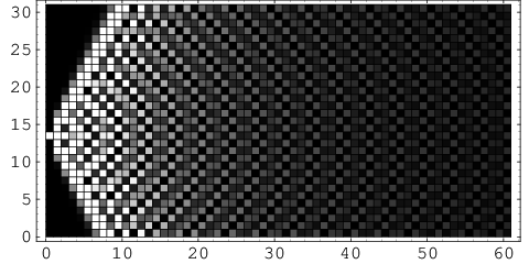
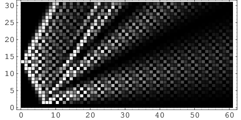
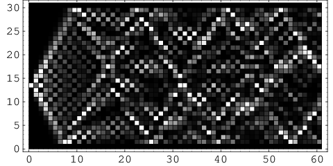
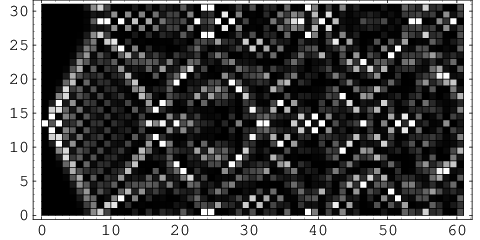
We use Theorems 1, 2 to create a plot of the probability densities for a quantum walk. In Figure 1 you see probability density plots that were made by truncating at the appropriate kk given by Theorem 2.

Refer to caption
(a) No boundaries
Refer to caption
(b) One boundary
Refer to caption
(c) Two boundaries
Refer to caption
(d) Periodic boundary conditions
Figure 1: Probabilities of a continuous-time quantum walk with x0=13x_{0}=13, L=0L=0, R=30R=30. For two or periodic boundary conditions, we chose a precision of 10−510^{-5}. Therefore we can truncate after k=12k=12 terms.

II Analysis of walks with no boundaries and one boundary

We can easily check that for k=1,…,N−1k=1,\ldots,N-1

|ψk⟩=2N∑x=L+1R−1sin(k​π​(x−L)N)|x⟩\left|\psi_{k}\right>=\sqrt{\frac{2}{N}}\sum_{x=L+1}^{R-1}\sin\left(\tfrac{k\pi(x-L)}{N}\right)\left|x\right>

are normalized and orthogonal eigenvectors of the matrix HqH_{q} defined in (3) with eigenvalues 2​cos⁡(k​πN)−q2\cos\big(\tfrac{k\pi}{N}\big)-q. Therefore we can write |ψ(t)⟩=ei​t​Hq|ψ(0)⟩\left|\psi(t)\right>=e^{itH_{q}}\left|\psi(0)\right> as

ψ⁡(x,t)=2N​∑k=1N−1sin⁡(π​k​(x−L)N)​ei​t​2​cos⁡(k​πN)−i​t​q×∑y=L+1R−1sin⁡(π​k​(y−L)N)​ψ​(y,0).\psi(x,t)=\frac{2}{N}\sum_{k=1}^{N-1}\sin\big(\tfrac{\pi k(x-L)}{N}\big)e^{it2\cos\big(\tfrac{k\pi}{N}\big)-itq}\\ \times\sum_{y=L+1}^{R-1}\sin\big(\tfrac{\pi k(y-L)}{N}\big)\psi(y,0).

Suppose we start the random walk at x0x_{0}, i.e. our starting state |ψ(0)⟩=|x0⟩\left|\psi(0)\right>=\left|x_{0}\right> or equivalently ψ⁡(x,0)=δx,x0\psi(x,0)=\delta_{x,x_{0}}. Then

ψ⁡(x,t)=2​e−i​t​qN​∑k=1N−1sin⁡(π​k​(x−L)N)​sin⁡(π​k​(x0−L)N)×ei​t​2​cos⁡(k​πN)=e−i​t​qN​∑k=1N−1cos⁡(π​k​|x−x0|N)​ei​t​2​cos⁡(k​πN)−e−i​t​qN∑k=1N−1cos(π​k​|x+x0−2​L|N)ei​t​2​cos⁡(k​πN)\begin{split}\psi(x,t)=&\frac{2e^{-itq}}{N}\sum_{k=1}^{N-1}\sin\big(\tfrac{\pi k(x-L)}{N}\big)\sin\big(\tfrac{\pi k(x_{0}-L)}{N}\big)\\ &\ \hskip 40.0pt\times e^{it2\cos\big(\tfrac{k\pi}{N}\big)}\\ =&\frac{e^{-itq}}{N}\sum_{k=1}^{N-1}\cos\big(\tfrac{\pi k|x-x_{0}|}{N}\big)e^{it2\cos\big(\tfrac{k\pi}{N}\big)}\\ &-\frac{e^{-itq}}{N}\sum_{k=1}^{N-1}\cos\big(\tfrac{\pi k|x+x_{0}-2L|}{N}\big)e^{it2\cos\big(\tfrac{k\pi}{N}\big)}\\ \end{split} (12)

We replace the sums with integrals. The error for these approximations are (see e.g. the errors for Newton-Cotes quadrature rules in isa-kel-66; note that the missing endpoints k=0,Nk=0,N can be added without penalties, since they cancel out in (12)):

|1N​[12​f​(0)+∑k=1N−1f⁡(kN)+12​f​(1)]−∫01f⁡(x)​dx|≤𝒪⁡(1N2​‖f′′​(x)‖∞),\left|\frac{1}{N}\left[\tfrac{1}{2}f(0)+\sum_{k=1}^{N-1}f(\tfrac{k}{N})+\tfrac{1}{2}f(1)\right]-\int_{0}^{1}f(x)\mathrm{d}x\right|\\ \leq\mathcal{O}\left(\frac{1}{N^{2}}\left\|f^{\prime\prime}(x)\right\|_{\infty}\right),

where the norm indicates the supremum of the second derivative of ff with respect to xx taken in the interval [0, 1][0,\,1]. Since for α,β≥0\alpha,\beta\geq 0

‖∂2∂w2​cos⁡(α​w)​ei​β​cos⁡w‖∞≤(α+β)2+β\left\|\frac{\partial^{2}}{\partial w^{2}}\cos\big(\alpha w\big)e^{i\beta\cos w}\right\|_{\infty}\leq(\alpha+\beta)^{2}+\beta

we can rewrite equation (12) as

ψ⁡(x,t)=e−i​t​q​∫01cos⁡(π​|x−x0|​w)​ei​t​2​cos⁡(π​w)​𝑑w−e−i​t​q∫01cos(π|x+x0−2L|w)ei​t​2​cos⁡(π​w)dw±e⁡(x,x0,t,N)\begin{split}\psi(x,t)=&\ e^{-itq}\int_{0}^{1}\cos(\pi|x-x_{0}|w)e^{it2\cos(\pi w)}\mathrm{d}w\\ &-e^{-itq}\int_{0}^{1}\cos(\pi|x+x_{0}-2L|w)e^{it2\cos(\pi w)}\mathrm{d}w\\ &\pm e(x,x_{0},t,N)\end{split}

with an error term of order

e⁡(x,x0,t,N)=𝒪⁡((|x−x0|+2​t)2+(|x+x0−2​L|+2​t)2N2).e(x,x_{0},t,N)=\mathcal{O}\left(\tfrac{(|x-x_{0}|+2t)^{2}+(|x+x_{0}-2L|+2t)^{2}}{N^{2}}\right). (13)

This representation allows us to express ψ⁡(x,t)\psi(x,t) as a sum of Bessel functions. According to abr-ste-72, equation 9.1.21, for n∈ℕ+n\in\mathbb{N}^{+} the Bessel function Jn​(z)J_{n}(z) is given by

Jn​(z)=i−nπ​∫0πei​z​cos⁡w​cos⁡(n​w)​𝑑wJ_{n}(z)=\frac{i^{-n}}{\pi}\int_{0}^{\pi}e^{iz\cos w}\cos(nw)\mathrm{d}w

and therefore J~n​(z)=1π​∫0πei​z​cos⁡w​cos⁡(n​w)​𝑑w\widetilde{J}_{n}(z)=\frac{1}{\pi}\int_{0}^{\pi}e^{iz\cos w}\cos(nw)\mathrm{d}w, and we can write

ψ⁡(x,t)=e−i​t​q​[J~|x−x0|​(2​t)−J~|x+x0−2​L|​(2​t)]±e⁡(x,x0,t,N).\begin{split}\psi(x,t)=&\ e^{-itq}\left[\widetilde{J}_{|x-x_{0}|}(2t)-\widetilde{J}_{|x+x_{0}-2L|}(2t)\right]\\ &\ \pm e(x,x_{0},t,N).\end{split} (14)

For R→∞R\rightarrow\infty, which implies N=R−L→∞N=R-L\rightarrow\infty, the error term e⁡(x,x0,t,N)e(x,x_{0},t,N) defined in (13) converges to 00 and we get

ψ⁡(x,t)=e−i​t​q​[J~|x−x0|​(2​t)−J~|x+x0−2​L|​(2​t)],\psi(x,t)=e^{-itq}\left[\widetilde{J}_{|x-x_{0}|}(2t)-\widetilde{J}_{|x+x_{0}-2L|}(2t)\right],\\

which proves (7). This is the limiting distribution for a continuous-time quantum random walk with one boundary. For no boundaries, i.e. if we let L→∞L\rightarrow\infty, too, (7) simplifies to

ψ⁡(x,t)=e−i​t​q​J~|x−x0|​(2​t),\psi(x,t)=e^{-itq}\widetilde{J}_{|x-x_{0}|}(2t),

since limn→∞Jn​(x)=0\lim_{n\rightarrow\infty}J_{n}(x)=0, which proves (7) and can be compared to the results from far-gut-98; kon-04.

III Walks with two boundaries

To derive the correct form of the quantum walk distribution for walks with two boundaries we check the correctness of Equation (6) for the unbounded case by plugging it into (1):

i​∂∂t​ψ​(x,t)=i​∂∂t​[i|x−x0|​e−i​t​q​J|x−x0|​(2​t)]=i​i|x−x0|​[−i​q​e−i​t​q​J|x−x0|​(2​t)+e−i​t​q​J|x−x0|′​(2​t)],i\frac{\partial}{\partial t}\psi(x,t)=i\frac{\partial}{\partial t}\left[i^{\left|x-x_{0}\right|}e^{-itq}J_{\left|x-x_{0}\right|}(2t)\right]\\ =ii^{|x-x_{0}|}\Big[-iqe^{-itq}J_{|x-x_{0}|}(2t)+e^{-itq}J^{\prime}_{|x-x_{0}|}(2t)\Big],

where we use that the derivative of the Bessel function satisfies Jν′​(z)=Jν−1​(z)−Jν+1​(z)2J^{\prime}_{\nu}(z)=\frac{J_{\nu-1}(z)-J_{\nu+1}(z)}{2}, see e.g. abr-ste-72, to verify that ψ\psi indeed fulfills (1), at least for |x−x0|≥1|x-x_{0}|\geq 1. In the special case |x−x0|=0|x-x_{0}|=0 we use that J0′​(z)=−J1​(z)J^{\prime}_{0}(z)=-J_{1}(z).

To satisfy the boundary conditions ψ⁡(L,t)=ψ⁡(R,t)=0\psi(L,t)=\psi(R,t)=0 we use the method of images, see mor-fes-53, and introduce mirror images of the walk starting at x0x_{0}. Let |ψx0(t)⟩\big|\psi_{x_{0}}(t)\big> be the solution for an unbounded walk starting at x0x_{0}. Then |ψx0(0)(t)⟩=|ψx0(t)⟩\big|\psi^{(0)}_{x_{0}}(t)\big>=\big|\psi_{x_{0}}(t)\big> is a good approximation to the solution, but we have to correct the error on the boundary by introducing walks starting at x−1=L−(x0−L)x_{-1}=L-(x_{0}-L) and x1=R+(R−x0)x_{1}=R+(R-x_{0}):

|ψx0(1)(t)⟩=|ψx0(0)(t)⟩−|ψx−1(t)⟩−|ψx1(t)⟩.\big|\psi^{(1)}_{x_{0}}(t)\big>=\big|\psi^{(0)}_{x_{0}}(t)\big>-\big|\psi_{x_{-1}}(t)\big>-\big|\psi_{x_{1}}(t)\big>.

To correct the error introduced by the corrections we continue to add mirror images at x−2=L−(x1−L)x_{-2}=L-(x_{1}-L) and x2=R+(R−x−1)x_{2}=R+(R-x_{-1}), …, until we arrive at (8). Let us check that

ψ⁡(L,t)e−i​t​q=∑n=−∞∞(−1)n​J~|L−xn|​(2​t)=∑n=0∞(−1)n​[J~|L−xn|​(2​t)−J~|L−x−(n+1)|​(2​t)]=∑n=0∞(−1)n​[J~|L−xn|​(2​t)−J~|xn−L|​(2​t)]=0,\begin{split}\frac{\psi(L,t)}{e^{-itq}}&=\sum_{n=-\infty}^{\infty}(-1)^{n}\widetilde{J}_{|L-x_{n}|}(2t)\\ &=\sum_{n=0}^{\infty}(-1)^{n}\left[\widetilde{J}_{|L-x_{n}|}(2t)-\widetilde{J}_{|L-x_{-(n+1)}|}(2t)\right]\\ &=\sum_{n=0}^{\infty}(-1)^{n}\left[\widetilde{J}_{|L-x_{n}|}(2t)-\widetilde{J}_{|x_{n}-L|}(2t)\right]=0,\end{split}

and similarly ψ⁡(R,t)=0\psi(R,t)=0. This proves (8).

For periodic boundary conditions ψ⁡(L,t)=ψ⁡(R,t)\psi(L,t)=\psi(R,t) we also build a solution starting from |ψx0(t)⟩\left|\psi_{x_{0}}(t)\right>. In order to enforce periodicity, we add two walks at y−1=x0−Ny_{-1}=x_{0}-N and y1=x0+Ny_{1}=x_{0}+N, which is the correction term for the “first round”. If we define

yn=x0+n​Ny_{n}=x_{0}+nN

we arrive at (10). Then

ψ⁡(L,t)e−i​t​q=∑n=−∞∞J~|L−yn|​(2​t)=∑n=−∞∞J~|L−n​N−x0|​(2​t)=∑n=−∞∞J~|R−(n+1)​N−x0|​(2​t)=ψ⁡(R,t)e−i​t​q,\begin{split}\frac{\psi(L,t)}{e^{-itq}}&=\sum_{n=-\infty}^{\infty}\widetilde{J}_{|L-y_{n}|}(2t)=\sum_{n=-\infty}^{\infty}\widetilde{J}_{|L-nN-x_{0}|}(2t)\\ &=\sum_{n=-\infty}^{\infty}\widetilde{J}_{|R-(n+1)N-x_{0}|}(2t)=\frac{\psi(R,t)}{e^{-itq}},\end{split}

which completes the proof of Theorem 1.

IV Approximations

For practical purposes the infinite series in Theorem 1 are unsatisfactory. Theorem 2, which we will prove in this section, fortunately tells us that we can truncate those series and still get an excellent approximation to the correct distribution.

Consider the distribution ψ⁡(x,t)\psi(x,t) in (8) for zero boundary conditions

ψ⁡(x,t)=e−i​t​q​∑n=−∞∞(−1)n​J~|x−xn|​(2​t),\psi(x,t)=e^{-itq}\sum_{n=-\infty}^{\infty}(-1)^{n}\widetilde{J}_{|x-x_{n}|}(2t),

and truncate it after the first kk terms. We would like to determine the error of this approximation, i.e.

ek,0=|ψ⁡(x,t)−e−i​t​q​∑n=−kk(−1)n​J~|x−xn|​(2​t)|,e_{k,0}=\left|\psi(x,t)-e^{-itq}\sum_{n=-k}^{k}(-1)^{n}\widetilde{J}_{|x-x_{n}|}(2t)\right|,

for t≥0t\geq 0. We can bound the Bessel functions Jν​(2​t)J_{\nu}(2t) by

|Jν​(2​t)|≤|t|νΓ⁡(ν+1),\left|J_{\nu}(2t)\right|\leq\frac{\left|t\right|^{\nu}}{\Gamma(\nu+1)}, (15)

see abr-ste-72. Then the error ek,0e_{k,0} is bounded by

ek,0≤∑n=k+1∞|J~|x−xn|​(2​t)|+∑n=−k−1−∞|J~|x−xn|​(2​t)|≤∑n=k+1∞[t|x−xn|Γ⁡(|x−xn|+1)+t|x−x−n|Γ⁡(|x−x−n|+1)].\begin{split}e_{k,0}\leq&\sum_{n=k+1}^{\infty}\left|\widetilde{J}_{|x-x_{n}|}(2t)\right|+\sum_{n=-k-1}^{-\infty}\left|\widetilde{J}_{|x-x_{n}|}(2t)\right|\\ \leq&\sum_{n=k+1}^{\infty}\left[\frac{t^{|x-x_{n}|}}{\Gamma(|x-x_{n}|+1)}+\frac{t^{|x-x_{-n}|}}{\Gamma(|x-x_{-n}|+1)}\right].\end{split}

We similarly define the kk term approximation error ek,pe_{k,p} for periodic boundary conditions.

From the definition (9) of the reflection points xnx_{n}

xn={L−(x−n−1−L)n<0R+(R−x−n+1)n>0x_{n}=\begin{cases}L-(x_{-n-1}-L)&n<0\\ R+(R-x_{-n+1})&n>0\end{cases}

we see that L+n​N≤xn≤R+n​NL+nN\leq x_{n}\leq R+nN. Therefore, and since L≤x≤RL\leq x\leq R,

ek,0≤∑n=k+1∞[t|x−xn|Γ⁡(|x−xn|+1)+t|x−x−n|Γ⁡(|x−x−n|+1)]≤∑n=k+1∞[t(n+1)​NΓ⁡((n−1)​N+1)+t(n+1)​NΓ⁡((n−1)​N+1)]≤2​tN​∑n=k+1∞tn​N((n−1)​N)!=2​t2​N​∑n=k∞tn​N(n​N)!.\begin{split}e_{k,0}\leq&\sum_{n=k+1}^{\infty}\left[\frac{t^{|x-x_{n}|}}{\Gamma(|x-x_{n}|+1)}+\frac{t^{|x-x_{-n}|}}{\Gamma(|x-x_{-n}|+1)}\right]\\ \leq&\sum_{n=k+1}^{\infty}\left[\frac{t^{(n+1)N}}{\Gamma((n-1)N+1)}+\frac{t^{(n+1)N}}{\Gamma((n-1)N+1)}\right]\\ \leq&2t^{N}\sum_{n=k+1}^{\infty}\frac{t^{nN}}{((n-1)N)!}=2t^{2N}\sum_{n=k}^{\infty}\frac{t^{nN}}{(nN)!}.\end{split} (16)

The same error estimate also holds for the error ek,pe_{k,p} of the kk-term approximation to the series (10) for periodic boundary conditions.

To estimate ek,0e_{k,0} and ek,pe_{k,p} in (16) we can use Stirling’s formula

x!=2​π​xx+12​e−x+θ12​x≥2​π​xx+12​e−x,x!=\sqrt{2\pi}x^{x+\frac{1}{2}}e^{-x+\frac{\theta}{12x}}\geq\sqrt{2\pi}x^{x+\frac{1}{2}}e^{-x},

see abr-ste-72, where x>0x>0 and 0<θ<10<\theta<1. Then

(n​N)!≥2​π​(n​N)(n​N)+12​e−(n​N)≥2​π​n​N​(n​N​e−1)n​N.\begin{split}(nN)!\geq&\sqrt{2\pi}(nN)^{(nN)+\frac{1}{2}}e^{-(nN)}\\ \geq&\sqrt{2\pi nN}(nNe^{-1})^{nN}.\end{split}

Therefore the error ek,0e_{k,0} from (16) is bounded by

ek,0≤2​t2​N2​π​N​∑n=k∞1n​[t​en​N]n​N≤2​t2​N2​π​N​k​∑n=k∞[t​en​N]n​N.e_{k,0}\leq\frac{2t^{2N}}{\sqrt{2\pi N}}\sum_{n=k}^{\infty}\frac{1}{\sqrt{n}}\left[\frac{te}{nN}\right]^{nN}\hskip-3.0pt\leq\frac{2t^{2N}}{\sqrt{2\pi Nk}}\sum_{n=k}^{\infty}\left[\frac{te}{nN}\right]^{nN}\hskip-3.0pt.

This series converges if k=k⁡(t,ε)k=k(t,\varepsilon) is chosen such that k>t​eNk>\frac{te}{N}. In this case

∑n=k∞(t​en​N)N​n≤(t​ek​N)N​k​∑n=k∞(t​ek​N)N⁡(n−k)=(t​ek​N)N​k​11−(t​ek​N)N=e−N​k​ln⁡k​Nt​e1−(t​ek​N)N.\begin{split}\sum_{n=k}^{\infty}\left(\frac{te}{nN}\right)^{Nn}\leq&\left(\frac{te}{kN}\right)^{Nk}\sum_{n=k}^{\infty}\left(\frac{te}{kN}\right)^{N(n-k)}\\ =&\left(\frac{te}{kN}\right)^{Nk}\frac{1}{1-\left(\frac{te}{kN}\right)^{N}}\\ =&\frac{e^{-Nk\ln\frac{kN}{te}}}{1-\left(\frac{te}{kN}\right)^{N}}.\end{split} (17)

Therefore the error from truncating after kk terms is

ek,0≤2​t2​N2​π​e​N​k​e−N​k​ln⁡k​Nt​e1−(t​ek​N)N\begin{split}e_{k,0}\leq&\frac{2t^{2N}}{\sqrt{2\pi eNk}}\frac{e^{-Nk\ln\frac{kN}{te}}}{1-\left(\frac{te}{kN}\right)^{N}}\end{split} (18)

We want to use (18) to find kk such that ek,0=𝒪⁡(ε)e_{k,0}=\mathcal{O}(\varepsilon). We make the following ansatz

k=\displaystyle k= k⁡(t,ε)=t+NN​ζln⁡ζ, where\displaystyle k(t,\varepsilon)=\frac{t+N}{N}\frac{\zeta}{\ln\zeta},\text{ where} (19)
ζ=\displaystyle\zeta= ζ⁡(t,ε)=2​ln⁡t+ln(cε−1t−1/2)N\displaystyle\zeta(t,\varepsilon)=2\ln t+\frac{\ln(c\,\varepsilon^{-1}t^{-1/2})}{N} (20)

with a constant c>0c>0 that we will determine. We have to check that the requirement k>t​eNk>\frac{te}{N} that guarantees convergence in (17) is fulfilled. If we restrict tt to

t≥(ee​(ε/c)1N)2​N4​N−1t\geq\left(e^{e}(\varepsilon/c)^{\frac{1}{N}}\right)^{\frac{2N}{4N-1}} (21)

then

ζ=2​ln⁡t+ln(cε−1t−1/2)N≥e.\zeta=2\ln t+\frac{\ln(c\,\varepsilon^{-1}t^{-1/2})}{N}\geq e. (22)

Additionally we observe that zln⁡z\frac{z}{\ln z} is growing monotonously for z>ez>e,

dd​z​zln⁡z=ln⁡z−1(ln⁡z)2>0​ for ​z>e,\frac{\mathrm{d}}{\mathrm{d}z}\frac{z}{\ln z}=\frac{\ln z-1}{(\ln z)^{2}}>0\text{ for }z>e,

and therefore for tt chosen as in (21)

k=t+NN​ζln⁡ζ≥t+NN​e>t​eN.\begin{split}k=&\frac{t+N}{N}\frac{\zeta}{\ln\zeta}\geq\frac{t+N}{N}e>\frac{te}{N}.\end{split} (23)

We estimate the numerator and denominator of ek,0e_{k,0} in (18) separately and write ek,0≤M⁡(k)D⁡(k)e_{k,0}\leq\frac{M(k)}{D(k)}. If we insert (19) into the numerator of (18), we see that

M⁡(k):=2​t2​N​e−N​k​ln⁡k​Nt​e=2​t2​N​e−N​t+NN​ζln⁡ζ​ln⁡(t+NN​ζln⁡ζ​Nt​e)=2​t2​N​e−(t+N)​ζ​(1+ln⁡t+Nt​e−ln⁡ln⁡ζln⁡ζ).\begin{split}M(k):=&2t^{2N}e^{-Nk\ln\frac{kN}{te}}=2t^{2N}e^{-N\frac{t+N}{N}\frac{\zeta}{\ln\zeta}\ln\left(\frac{t+N}{N}\frac{\zeta}{\ln\zeta}\frac{N}{te}\right)}\\ =&2t^{2N}e^{-(t+N)\zeta\left(1+\frac{\ln\frac{t+N}{te}-\ln\ln\zeta}{\ln\zeta}\right)}.\end{split}

Now we use that we can show that for z>1z>1

ln⁡t+Nt​e−ln⁡ln⁡zln⁡z≥ln⁡t+Nt​e−ln⁡ln⁡et+Ntln⁡et+Nt=−tt+N.\frac{\ln\frac{t+N}{te}-\ln\ln z}{\ln z}\geq\frac{\ln\frac{t+N}{te}-\ln\ln e^{\frac{t+N}{t}}}{\ln e^{\frac{t+N}{t}}}=-\frac{t}{t+N}.

We can use this to estimate M⁡(k)M(k) since ζ≥e>1\zeta\geq e>1, see (22), and get

M⁡(k)≤2​t2​N​e−ζ​N=2​t2​N​e−2​N​ln⁡t​eln⁡(c−1​ε​t1/2)=2c​ε​t.M(k)\leq 2t^{2N}e^{-\zeta N}=2t^{2N}e^{-2N\ln t}e^{\ln(c^{-1}\varepsilon t^{1/2})}=\frac{2}{c}\varepsilon\sqrt{t}.

To estimate the denominator of (18)

D⁡(k):=2​π​e​N​k​(1−(t​ek​N)N)D(k):=\sqrt{2\pi eNk}\left(1-\left(\frac{te}{kN}\right)^{N}\right)

we insert (19) in

t​ek​N=t​et+NN​ζln⁡ζ​N=tt+N​e​ln⁡ζζ.\frac{te}{kN}=\frac{te}{\frac{t+N}{N}\frac{\zeta}{\ln\zeta}N}=\frac{t}{t+N}\frac{e\ln\zeta}{\zeta}. (24)

We can see that both tt+N\frac{t}{t+N} and e​ln⁡ζζ\frac{e\ln\zeta}{\zeta} are less than 11 for tt as in (21), when we have ζ≥e\zeta\geq e, see (22). We analyze (24) by considering t∈[(ee​(ε/c)1N)2​N4​N−1,∞)t\in[(e^{e}(\varepsilon/c)^{\frac{1}{N}})^{\frac{2N}{4N-1}},\,\infty) over two intervals. For t∈[(ee​(ε/c)1N)2​N4​N−1, 10)t\in[(e^{e}(\varepsilon/c)^{\frac{1}{N}})^{\frac{2N}{4N-1}},\,10)

tt+N​e​ln⁡ζζ≤tt+N≤tt+1≤1011.\frac{t}{t+N}\frac{e\ln\zeta}{\zeta}\leq\frac{t}{t+N}\leq\frac{t}{t+1}\leq\frac{10}{11}.

In the interval [10,∞)[10,\,\infty) we use that e​ln⁡ζζ\frac{e\ln\zeta}{\zeta} converges monotonously to 00 for ζ=ζ⁡(t,ε)→∞\zeta=\zeta(t,\varepsilon)\rightarrow\infty, and that ζ≥2​ln⁡t\zeta\geq 2\ln t:

tt+N​e​ln⁡ζζ≤e​ln⁡ζζ≤e​ln⁡(2​ln⁡t)2​ln⁡t≤0.902≤1011.\frac{t}{t+N}\frac{e\ln\zeta}{\zeta}\leq\frac{e\ln\zeta}{\zeta}\leq\frac{e\ln(2\ln t)}{2\ln t}\leq 0.902\leq\frac{10}{11}.

Therefore we can use this and (23) for

D⁡(k)≥2​π​e​N​k​111>e​2​π​t11.D(k)\geq\sqrt{2\pi eNk}\frac{1}{11}>\frac{e\sqrt{2\pi t}}{11}.

If we combine the results for numerator and denominator, we can estimate

ek,0≤M⁡(k)D⁡(k)≤22c​e​2​π​ε,e_{k,0}\leq\frac{M(k)}{D(k)}\leq\frac{22}{ce\sqrt{2\pi}}\varepsilon,

and we see that we have to choose c:=22e​2​πc:=\frac{22}{e\sqrt{2\pi}}. This result holds for all tt chosen according to (21).

If we follow the same steps we can also estimate the error ek,pe_{k,p} of a kk term approximation for periodic boundary conditions. This proves Theorem 2.

V Acknowledgments

The author would like to thank the members of the Institute for Quantum Computing and the University of Waterloo for their hospitality and many intriguing discussions. Special thanks to Michele Mosca, Hilary Carteret and Bruce Richmond for helpful comments. The author would also like to thank David DiVincenzo for pointing out the description of the method of images in mor-fes-53 to him and Henryk Woźniakowkski for his advice regarding the convergence rate of the power series.

References

  • [1] M. Abramowitz and I. A. Stegun. Handbook of Mathematical Functions. Dover, 1972.
  • [2] D. Aharonov, A. Ambainis, J. Kempe, and U. Vazirani. Quantum walks on graphs. In Proceedings of the 33rd annual ACM symposium on Theory of computing (STOC ’01), pages 50–59, New York, NY, USA, 2001. ACM Press. quant-ph/0012090.
  • [3] A. Ambainis. Quantum walks and their algorithmic applications. International Journal of Quantum Information, 1:507–518, 2003. quant-ph/0403120.
  • [4] B. Apolloni and D. de Falco. The clock of a quantum computer. Journal of Physics A, 35:10033–10051, 2002.
  • [5] A. Childs, E. Farhi, and S. Gutmann. An example of the difference between quantum and classical random walks. Quantum Information Processing, 1:35, 2002.
  • [6] E. Farhi and S. Gutmann. Quantum computation and decision trees. Physical Review A, 58:915–918, 1998.
  • [7] H. Gerhardt and J. Watrous. Continuous-time quantum walks on the symmetric group. In Lecture Notes in Computer Science, volume 2764, pages 290–301, 2003.
  • [8] A. D. Gottlieb. Convergence of continuous time quantum walks on the line. quant-ph/0409042, 2004.
  • [9] T. Gramss. Solving the schrödinger equation for the feynman quantum computer. International Journal of Theoretical Physics, 37(5):1423–1439, 1998.
  • [10] E. Isaacson and H. B. Keller. Analysis of Numerical Methods. Wiley, 1966.
  • [11] J. Kempe. Quantum random walks: an introductory overview. Contemp. Phys., 44(4), 2003. quant-ph/0303081.
  • [12] N. Konno. Continuous-time quantum walk on the line. Physical Review E, 72:026113, 2005.
  • [13] D. A. Meyer. From quantum cellular automata to quantum lattice gases. Journal of Statistical Physics, 85:551–574, 1996. quant-ph/9807070.
  • [14] P. M. Morse and H. Feshbach. Methods of theoretical physics. Mc Graw-Hill, 1953.
  • [15] O. Mülken and A. Blumen. Continuous time quantum walks in phase space. Phys. Rev. A, 73:012105, 2006.
  • [16] F. W. Strauch. Relativistic quantum walks. quant-ph/0508096, 2005.