Opacity of electromagnetically induced transparency for quantum fluctuationsPreprint: APS/123-QED

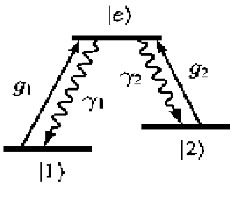
Electromagnetically induced transparency (EIT) rv:harris is a technique that can be used to eliminate fluorescence from an atom illuminated with light whose frequency is equal to a particular atomic transition. This technique can be used in systems of three-level atoms in $\Lambda$ configuration rv:marangos, see Fig. 1. In this configuration a mode of the field, called the pump field, interacts resonantly with one dipole transition, while another mode, the probe field, interacting with the second dipole transition, is tested for transparency. The linear response of the absorption of the probe field by the medium is described by the imaginary part of the electric susceptibility. In Fig. 2 we plot the susceptibility as a function of the probe frequency (solid line). The maximum absorption of the probe field by the medium depends on the Rabi frequencies associated with each atomic optical transition. The maximum occurs for a detuning from resonance which increases monotonically with the Rabi frequencies.

Many recent works have investigated if this transparency, originally studied for classical fields, preserves the initial quantum properties of the probe field. For a classical pump field with Rabi frequency much larger than that of the probe, Lukin et al. rv:memoria2 showed that the medium is transparent for the quantum state. Furthermore, they demonstrated a transfer of the initial quantum state from the probe field to the atoms and in a second stage back to the field by varying the Rabi frequency of the pump laser. They proposed using this technique as a quantum memory device. When both fields are treated quantum mechanically, Dantan et al. rv:dantan4 studied the noise spectrum of the quadratures, when only the coherent pump field drives the atoms and the probe field is initially in a broad-band squeezed vacuum. If the frequency equals that of the atomic transition, the medium is transparent. For other frequencies, there is absorption of the quantum properties. The spectral absorption varies in a similar manner as the transparency curve for the mean value of the field. The transparency for the vacuum squeezed state was confirmed experimentally by Akamatsu et al. rv:kozuma.

In this Letter, we discuss the propagation of a quantum state in a medium of three level atoms showing EIT in the stationary regime. We focus on the case of a squeezed initial state of the probe field and a coherent pump field. We treat both fields quantum mechanically and in contrast to previous work we do not put any constraint on the probe Rabi frequency. An analytical solution is given for this general case. Our main result is that the absorption of the initial squeezing is accompanied by an oscillatory interchange of the quantum properties between the pump and probe field while traveling through the medium. This oscillatory behavior is present for frequencies where the absorption of the mean value of the field is usually negligible. The effect is maximally pronounced for the case of equal Rabi frequencies. As a consequence, the probe and pump states after propagation can be completely different from the input state.

To probe the behavior of quantum fluctuations of light passing through an EIT–medium, we use squeezed states defined by $|{\alpha;\xi}\rangle\equiv D(\alpha)S(\xi)|{0}\rangle$ with the squeezing operator $S(\xi)=\exp[(\xi{a^{\dagger}}^{2}-\xi^{\ast}a^{2})/2]$ and displacement operator $D(\alpha)=\exp[\alpha a^{\dagger}-\alpha^{\ast}a]$, where $a$ and $a^{\dagger}$ are the annihilation and creation operator of the mode under consideration. After propagation along the $z$–axis, we analyze the fluctuation spectrum

in the steady state of the quadrature fluctuation $\delta Y^{\theta}(t)=\delta a(t)\exp(-i\theta)+\delta a^{\dagger}(t)\exp(i\theta)$, where $\delta a=a-\langle a\rangle$.

We consider two quasi monochromatic one dimensional beams of light propagating along the $z$ axis in a medium of $N$ three-level atoms in $\Lambda$-configuration. The excited state $|{e}\rangle$ of the atom with total linewidth $\gamma=\gamma_{1}+\gamma_{2}$ can decay spontaneously with rate $\gamma_{j}$ into the lower electronic state $|{j}\rangle$ ($j=1,2$). To describe the propagation of the two beams, we use a multimode representation of a pair of electromagnetic fields $\vec{E}_{j}=\vec{\mathcal{E}}_{j}a_{j}(z,t)\exp[ik_{{\rm L},j}z-\omega_{{\rm L},j}t]+{\rm h.c.}$ and treat the medium in a continuum approximation bib:fleisch95; rv:dantan4. Here, $|\vec{\mathcal{E}}_{j}|$ is the vacuum electric field at the laser’s carrier frequency $\omega_{{\rm L},j}=ck_{{\rm L},j}$, and $a_{j}(z,t)$ is the envelope operator of the corresponding field $j$, which is slowly varying in space and time. For the medium we assume the inter-atomic distance to be much smaller than the shortest relevant wave length of the laser light and introduce the continuous atomic operators $\sigma_{\mu\nu}(z)=\lim_{\Delta z\rightarrow 0}\frac{L}{N\Delta z}\!\sum\limits_{z^{(j)}\in\Delta z}\!\sigma_{\mu\nu}^{(j)}$, where $\sigma^{(j)}_{\mu\nu}=|{\mu}\rangle^{(j)}\langle{\nu}|$ is the individual atomic operator of atom $j$ at position $z_{j}$.

The atoms interact with the electric fields via their dipole moment $\wp$; we treat this interaction in the rotating wave approximation. Then, in the slowly varying envelope approximation, the Heisenberg equation of motion for the field operator $a(z,t)$ gives

where we have introduced the coupling constant $g_{j}=\vec{\wp}\vec{\mathcal{E}}_{j}/\hbar$. Using the inversion operators $\varpi_{j}=\sigma_{ee}-\sigma_{jj}$, the Heisenberg-Langevin equations of the atomic degree of freedom for resonant driving read

This system of equations (2a) and (2b) is easily interpreted: The polarization field $\sigma_{je}(z,t)$ serves as a source for the electric fields, whereas the propagating light in turn drives the atomic media via the dipole interaction terms $\propto g_{j}$. The $f_{j}$ are delta-correlated, collective Langevin operators which account for the noise introduced by the coupling of the atomic system to the free radiation field. They have vanishing mean values and correlation functions of the form $\langle f_{x}(z,t)f_{y}(z,t^{\prime})\rangle=\frac{L}{N}D_{xy}\delta(t-t^{\prime})\delta(z-z^{\prime})$. The diffusion coefficients $D_{xy}$ can be obtained from the generalized Einstein equations bib:louisell. For this particular problem they are listed in bib:pablonicim

We will use the common technique bib:davidov; bib:louisell of transforming Eqs. (2a) and (2b) into stochastic c-number equations which serve to calculate correlation functions of the atomic and field operator up to second order. To fix the corresponding order of operators we use the “normal” order convention $a_{2}^{\dagger},a_{1}^{\dagger},{\sigma}_{e2},{\sigma}_{e1},{\sigma}_{12},\varpi_{1},\varpi_{2},\sigma_{21},\sigma_{1e},\sigma_{2e},a_{1},a_{2}$. All calculated results from the c-number equations have to be considered to represent the results using operators in this order. The equations of motion for the c-number quantities are equivalent to those for the operators, except that a redefinition of the diffusion coefficients is necessary. These new diffusion coefficients are listed in bib:pablonicim. In the following, we use the same symbols for operators and their c-number substitutions, except that for the field operators $a_{j}$ we instead use $\alpha_{j}$.

In order to solve the c-number counterparts of Eqs. (2a) and (2b), it is convenient to collect the system quantities and the fluctuation forces in vectors $\mathbf{x}^{\rm T}(z,t)=(\alpha_{2}^{\ast},\alpha_{1}^{\ast},{\sigma}_{e2},\dots,\sigma_{2e},\alpha_{1},\alpha_{2})$ and $\mathbf{f}^{\rm T}(z,t)=(0,0,f_{e2},\dots,f_{2e},0,0)$, where for the components we choose the same order convention introduced above. For a large number of atoms, it is reasonable to assume a steady state for the mean values $\langle\mathbf{x}\rangle$ with small fluctuations $\delta\mathbf{x}$, i.e. we write $\mathbf{x}=\langle\mathbf{x}\rangle+\delta\mathbf{x}$. This allows us to treat the problem perturbatively for small fluctuations $\delta\mathbf{x}\propto O(1/\sqrt{N})$ bib:davidov; bib:stochasticmethods. The steady state values $\langle\mathbf{x}\rangle\propto O(1)$ are found from the equations of motion (2a) and (2b) to zeroth order in $\delta\mathbf{x}$, after setting all time derivatives to zero. Due to EIT the steady state values are $z$-independent. To first order, the system of equations

is linear in the fluctuations, where $\delta\mathbf{x}(s,t)=\int\limits_{0}^{\infty}\exp[-sz]\delta\mathbf{x}(z,t)dz$ (and analogously for $\mathbf{f}$) denotes the Laplace transform of $\delta\mathbf{x}(z,t)$. The elements of the matrix ${\mathcal{M}}(s)$ are calculated from the equations (2a) and (2b) to first order in $\delta\mathbf{x}$. In $\mathbf{g}(t)$ we collect the initial conditions at $z=0$ following from the Laplace transform of Eqs. (2a). Equation (3) can be cast into algebraic form using the Fourier transform $\delta\mathbf{x}(s,\omega)=\int\limits_{-\infty}^{\infty}dt\,\exp[-i\omega t]\delta\mathbf{x}(s,\omega)/\sqrt{2\pi}$. From the solution $\delta\mathbf{x}(s,\omega)=[{\mathcal{M}}+i\omega]^{-1}(\mathbf{f}+\mathbf{g})$ we can construct the correlation matrix

with ${\mathcal{D}}\delta(\omega+\omega^{\prime})=\langle\mathbf{f}\mathbf{f^{\dagger}}\rangle$, ${\mathcal{G}}\delta(\omega+\omega^{\prime})=\langle\mathbf{g}\mathbf{g^{\dagger}}\rangle$ and $\langle\mathbf{f}\mathbf{g^{\dagger}}\rangle=\langle\mathbf{g}\mathbf{f^{\dagger}}\rangle=0$. For fields entering the medium in a squeezed state with real squeezing parameter $\xi_{j}$ ($j=1,2$), we have

with all other coefficients of ${\mathcal{G}}$ vanishing.

We can now use the result (4) to calculate the spectrum of fluctuations of the electric fields. To this end we recall the relation

following from the Wiener Khinchine theorem, connecting the fluctuation spectrum $S_{j}(\omega)$, Eq. (1), with the correlation of the quadrature fluctuations $\delta Y_{j}^{\theta}(z,\omega)=\delta\alpha_{j}(z,\omega)e^{-i\theta}+\delta\alpha_{j}^{\ast}(z,-\omega)e^{i\theta}$. Recall that the c-number result represents the normal ordered spectrum neglecting vacuum fluctuations. To take these into account, we write $[{\mathcal{S}}_{j}(\omega)-1]$ in Eq. (7) in order to ensure that ${\mathcal{S}}_{j}(\omega)=1$ for a coherent state. The spectrum ${\mathcal{S}}_{j}(\omega)$ can now be calculated by evaluating the left-hand side of Eq. (7) with the help of the corresponding matrix elements from Eq. (4) using a two-dimensional inverse Laplace transform in $s$ and $s^{\prime}$.

As initial conditions we specify $\xi_{1}=0$ and real $\xi_{2}=\xi$, that is, the probe field ($j=2$) is in a broad band squeezed state, whereas the pump field is coherent. All frequency components of both pump and probe beam, are in a squeezed/coherent vacuum ($\alpha_{j}=0$ for $\omega\neq\omega_{\rm L}$), only the carrier frequencies of the two beams are displaced by real $\alpha_{j}$, thus driving resonantly the atomic transitions with Rabi frequency $\Omega_{j}=|g_{j}\alpha_{j}|$.

Using these initial conditions, we find for the fluctuation spectra of pump ($j=1$) and probe ($j=2$)

with the resonance curve

Furthermore, we have defined $f(\xi,\theta)=1-e^{2\xi}\cos^{2}\theta-e^{-2\xi}\sin^{2}\theta$ and $\Omega^{2}=\Omega_{1}^{2}+\Omega_{2}^{2}$. Indeed, for $z=0$, we find ${\mathcal{S}}_{1}(0,\omega)=1$ and ${\mathcal{S}}_{2}(0,\omega)=e^{2\xi}$ for the $\theta=0$ quadrature. In Fig. 3 (a) we have plotted the fluctuation spectrum of the probe pulse as a function of frequency and propagation length $z$. In parts (b) and (c) of Fig. 3 cuts along the $\omega$ and $z$ direction are shown for both, pump and probe fields.

We start the discussion of Eqs. (8) and (9) with analyzing their asymptotic behavior. For $z\rightarrow\infty$ we obtain

The distance where this asymptotic behavior is achieved is governed by the exponentials in Eqs. (8) and  (9), and is of the order of $z_{\rm abs}=1/\gamma P(\omega,0)$. When $\Omega_{1}\neq 0$, the asymptotic quadrature fluctuations of the probe show absorption of the initial squeezing of the field. As $P(\omega,0)$ follows qualitatively the probe field mean value transparency curve, see Fig. 2, so does the distance where this asymptotic behavior takes place. The pump field shows also squeezed fluctuations in this limit, but from the analysis of different quadratures $\theta$ it follows that the state is no longer a minimum uncertainty state. For equal Rabi frequencies $\Omega_{1}=\Omega_{2}$, both fields have asymptotically the same fluctuations. Similar correlations are known in cavity EIT bib:agarwal and from the effect of pulse-matching bib:harris; bib:fleisch.

In the case of strong asymmetric driving $\Omega_{2}\ll\Omega_{1}$, it follows from Eqs. (8) and  (9) that the pump field always stays in a coherent state while the initial fluctuations of the probe field are exponentially damped during propagation through the medium. The intensity of the absorption is given by $\gamma P(\omega,0)$. As already mentioned, $P(\omega,0)$ behaves like the mean value transparency curve, so that we find a comparable behavior of the absorption of the probe’s quadrature fluctuations as for its mean value absorption. Thus, in this limit, our result reproduces the analysis reported in Ref. rv:dantan4.

When $\Omega_{1}\approx\Omega_{2}$, however we find an entirely novel behavior. In order to bring out this new aspect most clearly, we assume $\gamma P(\omega,0)z\ll 1$, that is, we consider positions $z$ where the exponential absorption of the quadrature fluctuations can be neglected. Then, Eqs. (8) and  (9) can be approximated as

with $\zeta=z/z_{\rm osc}$, where we introduce the oscillatory length scale $z_{\rm osc}=2/P(\omega,\Omega)\omega$. Equations (11) and (12) clearly display the oscillatory transfer of the initial quantum properties of the probe to the pump and back while traveling through the medium. During this oscillatory behavior, the pump and probe field stay in a minimum uncertainty state. Also the sum of the fluctuations ${\mathcal{S}}_{1}+{\mathcal{S}}_{2}$ is conserved. When $\Omega_{1}=\Omega_{2}$, this oscillatory transfer is maximal and all the fluctuation properties oscillate between the probe and the pump field during propagation in the medium. The length scale of the oscillatory transfer $z_{\rm osc}$ can be much smaller than the absorption length scale $z_{\rm abs}$. In Fig. 3, the interplay of both scales, oscillatory and absorption, can be clearly observed.

The oscillatory behavior implies that the outgoing quantum field can be completely different from the incoming field, although the mean values stay exactly the same. In other words, the medium is not transparent for the quantum properties of the field, at least not in the sense that the quantum state can traverse the medium unaltered. The oscillatory behavior is qualitatively different from the absorption and is “coherent” since it does not imply loss of quantum properties.

To check if these oscillations still persist with a damping rate $\Gamma_{12}$ of the ground state coherence we performed a numerical simulations. For a typical value $\Gamma_{12}=1/500\gamma$ the resulting curve (dotted) shown in Fig. 3 b) almost coincide with the ideal case. A complete discussion of the effect of decoherence will be published elsewhere.

Present technology allows for an experimental observation of this effect. The initial state can be constructed by mixing a laser tuned to the probe optical transition with a wide band squeezed field which covers the transparency window. With a Rabi frequency $\Omega_{1}=\Omega_{2}=\gamma$ and an observation frequency $\omega\approx 0.1\gamma$, $z_{\rm abs}$ is ten times $z_{\rm osc}$. For a density $\rho\approx 10^{9}$, we have a maximum transfer of quantum properties between the fields for $z\approx 7$cm, while $z_{\rm abs}\approx 70$cm. When $\omega\approx 0.25\gamma$ we have a maximum transfer of quantum properties between the fields for $z\approx 4.5$cm ($zC/\gamma\approx 25$ in Fig. 3 b)) while $z_{\rm abs}\approx 12$cm ($zC/\gamma\approx 64$). Parameters on this order are found in various EIT experiments rv:kozuma; rv:lukincollo; rv:rmpfleisch.

In conclusion, we have shown that in the propagation of pump and probe beams through an EIT medium, the quantum states are not conserved, except for the carrier frequencies which drive the atoms on two-photon resonance. Apart from absorption of quantum fluctuations, which takes place in approximately the same frequency range as the absorption of the mean values, we found a novel characteristic behavior, which is most strongly pronounced if the two beams have comparable Rabi frequencies, consisting of an oscillatory transfer of the initial quantum properties between the probe and the pump field. This effect could be observed in current state-of-the-art experiments.