Ellipses of Constant Entropy in the Spin Chain
Abstract
Entanglement in the ground state of the model on the infinite chain can be measured by the von Neumann entropy of a block of neighboring spins. We study a double scaling limit: the size of the block is much larger than but much smaller than the length of the whole chain. The entropy of the block has an asymptotic limit. We study this limiting entropy as a function of the anisotropy and of the magnetic field. We identify its minima at product states and its divergencies at the quantum phase transitions. We find that the curves of constant entropy are ellipses and hyperbolas and that they all meet at one point (essential critical point). Depending on the approach to the essential critical point the entropy can take any value between and . In the vicinity of this point small changes in the parameters cause large change of the entropy.
pacs
03.65.Ud, 02.30.Ik, 05.30.Ch, 05.50.+q1 Introduction
Entanglement is a primary resource for quantum information processing [1, 2, 3, 4]. It shows how much quantum effects we can use to control one system by another. Stable and large scale entanglement is necessary for scalability of quantum computation [5, 6]. The entropy of a subsystem as a measure of entanglement was discovered in [3]. Essential progress has been achieved in the understanding of entanglement in various quantum systems [5, 7, 8, 9, 10, 11, 12, 13, 14, 15, 16, 17, 18, 19, 20, 21, 22, 23, 24, 25, 26, 27, 28, 29].
The importance of the model for quantum information was emphasized in [14, 30, 31, 32]11 1 It is interesting to note that the critical behavior of the model is similar to the Lipkin-Meshkov-Glick model [19].. In this paper we consider the entropy of a block of neighboring spins in the ground state of the model [on the infinite chain] in the limit . We use the results of [33, 34, 35] and extend them to the whole phase diagram of the model.22 2 Moreover, in the Appendix we explain how these results can be used to calculate the entanglement of the model in a staggered magnetic field. The Hamiltonian of the model is
| (1) |
Here is the anisotropy parameter; , and are the Pauli matrices and is the magnetic field. The model is clearly symmetric under the transformation or . In [33, 35] only the case was discussed, here we can confirm that those results can be directly extended for by analytical continuation.
The model was solved in [36, 37, 38, 39]. The methods of Toeplitz determinants and integrable Fredholm operators were used for the evaluation of correlation functions, see [38, 40, 41, 42, 43, 44]. The idea to use the determinants for the calculation of the entropy was put forward in [16].
The solution of the model looks differently in three cases:
Case is defined by : This is strong magnetic field.
Case a is defined by and : Moderate magnetic field for small anisotropy, and includes zero magnetic field for large anisotropy.
Case b is defined by and : It describes weak magnetic field, including zero magnetic field in the small anisotropy regime.
At and for the model is known as the isotropic model (or XX model) and its spectrum is gapless. The entropy for this critical phase was calculated in [16]. The boundary between cases and a () is also critical. In the rest phase diagram, the spectrum of the model is given by:
| (2) |
We draw the phase diagram and the three cases we are considering in Fig. 1.
At the boundary between cases a and b () the ground state can be expressed as a product state as it was discovered in [45]. The ground state is in fact doubly degenerated:
| (3) |
Here . The role of factorized states was emphasized in [40, 46, 47]. Let us mention that the rest of the energy levels are separated by a gap and correlation functions decay exponentially. The boundary between cases a and b is not a phase transition.
2 Block Entropy
In general, we denote the ground state of the model by . We consider the entropy of a block of neighboring spins: it measures the entanglement between the block and the rest of the chain [3, 30]. We treat the whole ground state as a binary system . The block of neighboring spins is subsystem A and the rest of the ground state is subsystem B. The density matrix of the ground state is . The density matrix of the block is . The entropy of the block is:
| (4) |
Note that each of the ground states (3) is factorized and has no entropy.
To express the entropy we need the complete elliptic integral of the first kind,
and the modulus
| (5) |
The magnetic field and anisotropy define the elliptic parameter :
vanishes at large magnetic fields (), at for and at the boundary between case a and b (). In all these regions of the phase diagram, the ground state of the system is given by product states (a ferromagnetic state in the first two cases, the doubly degenerate state (3) for the latter). At the phase transitions ( and , ) the elliptic parameter .
In the paper [33] we used determinant representation for the evaluation of the entropy. The zeros of the determinant form an infinite sequence of numbers:
| (10) |
here in Case 1 and in Case 2. Note and as
These zeros allowed us to represent the entropy as a convergent series in [33]:
| (11) |
I. Peshel also obtained the series (11) in cases of non-zero magnetic field, see [34].33 3 In comparing with the results of [34], the reader should keep in mind that Peshel calculated the entropy per boundary, therefore his results differ by a factor of 2 compared to the ones in this paper. He summed it up into:
| Case | (12) | ||||
| Case a | (13) |
In our paper [33], we have shown that equation (11) is valid for all three cases, which allowed us to sum up the series (11) in case of weak magnetic field (including zero magnetic field) as well:
| (14) |
The rigorous proof and the precise history is given in the paper [35]. Here we report that these results are valid also for .
3 Entropy’s analysis
Now we can study the range of variation of the limiting entropy. We find a local minimum at the boundary between cases a and b (). This is the case of doubly degenerated ground state (3) and it is consistent with [48], where it was shown that when the ground state becomes a superposition of two product states with different quantum numbers, then the entropy of a subsystem turns into .
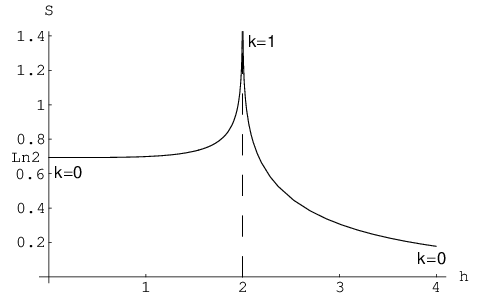
The absolute minimum () is achieved at infinite magnetic field or at for , where the ground state becomes ferromagnetic (i.e. all spins are parallel). The entropy diverges to , i.e has singularities, at the phase transitions: or . To show this behavior of the limiting entropy, we plot it as a function of the magnetic field at constant anisotropy in Fig. 2.
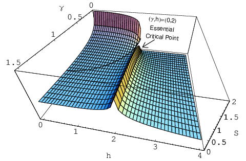
We provide a plot of the entropy as a function of at constant (vanishing) magnetic field () in Fig. 3, where the local minimum is again visible at . Figure 4 is a three-dimensional plot of the entropy as a function of both the anisotropy parameter and of the external magnetic field and all the feature discussed so far are visible.
The Ising point. The degenerate product states case (3) is particularly interesting. For , , the model reduces to the Ising model and the ground state (3) is given by the Bell-Pair state:
| (15) |
We plot the entropy as a function of the magnetic field at the Ising point in Fig. 5. One can notice that the local minimum is achieved at .
(a):
(b):

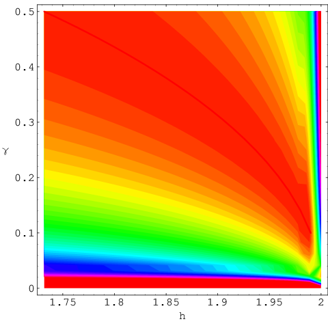
The essential critical point. Another interesting limit is reached around the point , . This point belongs to both of the critical phases of the model, so the entropy does not have an analytical expression [fixed value] on this point, but we can study the behavior of in vicinity of this point. We already studied a couple of trajectories reaching this critical point: along the boundary between cases a and b () the entropy is on its local minimum . Along the critical lines ( and for ) the entropy is divergent, while for and the ground state is ferromagnetic and the entropy is . Since the limit of the entropy reaching the point does not exist (it is direction-dependent), we call this point essential critical point. In the next section we study the vicinity of this point and show that depending on the direction of approach the entropy can take any positive value. In Fig. 6 we present a contour plot of the entropy around the essential critical point. From this plot one can see that the entropy can assume a wide range of values near the point.
4 Ellipses and hyperbolas of constant entropy
We now look for curves of constant entropy. Since the entropy depends only on the elliptic parameter (2), curves of constant entropy are curves of constant . Such trajectories are easily found and the family of curves of constant entropy can be written in terms of a single parameter :
| (16) | |||||
For (Case ), the curves of constant entropy are hyperbolas, while for (Case a and b) they are ellipses.
Each point in the phase diagram of the model belongs to one of these curves. By selecting a value of the parameter , we select a family of point with the same elliptic parameter in (2). There is a one-to-one correspondence between and :
| Case | (23) | ||||
| Case a | (24) | ||||
| (25) |
We recognize that , as the boundary between Case a and b, is the curve where the ground state can be expressed as a doubly degenerate product state (3).
It is important to notice that this curves have all the essential critical point in common. This means that starting from any point in the phase diagram of the model, one always reaches the essential critical point by following a curve of constant entropy.
For , the entropy has a minimum at and diverges to approaching the critical line . For , decreases monotonically from near the critical line to at infinite magnetic field. Beside the critical lines, the entropy is a continuous function, so its range is the positive real axis.
This means that, depending on the direction of approach, the entropy assumes every positive number near the essential critical point, since every ellipse or hyperbola of constant entropy passes through that point. In other words, a small deviation from the essential critical point can bring a big change in the value of the entropy. This is very important from the point of view of quantum control, because it allows to change dramatically the entanglement (and hence the quantum computing capabilities) with small changes in the parameters of the system.
It is easy to express the entropy in terms of the parameter defining the ellipses and hyperbolas of constant entropy:
| Case | ||||
| Case a | ||||
5 Entropy approaching the critical lines
Using the formulae of the previous section, we are now in a position to discuss the divergences of the entropy near the critical phases. General results exist in these cases, based on a conformal field theory approach [20] and specific results were derived for the isotropic case () in [16]. We know that, in the double-scaling limit we are considering, the entropy diverges logarithmically with the size of the block. The coefficient of this logarithmical divergence can be calculated by knowing the central charge of the corresponding conformal field theory at the critical point [20].
Setting or , the ellipses and hyperbolas of constant entropy (4) collapse into the critical lines, i.e. a vertical line at or a horizontal line at , respectively. Using (), we can study how the entropy diverges approaching these lines. Using Case b in (), we can take to find
| (27) | |||||
which is consistent with the results obtained in [16] for the isotropic case ().
We can investigate how the entropy approaches the critical line from below and from above. In the former case, we shall set in Case a of ():
| (28) | |||||
In the latter case, for a direction almost parallel to the critical line , but slightly above it, we take in Case of ():
| (29) | |||||
These results are in agreement with the conclusion of [20].
| Region | |||
|---|---|---|---|
| : | |||
| a: | |||
| b: | |||
6 Conclusions
We analyzed the entanglement in the ground state of the model on the infinite chain by studying the von Neumann entropy of a block of neighboring spins. This entropy is an effective measure of the quantum computing capabilities of a system and plays a fundamental role in the field of quantum information.
Using previously known results for the entropy in the limit of a large block of spins [35]-[33], we studied the behavior of in the phase diagram of the model (see Table 1). We found that for , the entropy has a local minimum on the curve . On this line the ground state is a doubly degenerate linear combination of product states. The entropy diverges to at the phase transitions and , . For , the entropy reaches the absolute minimum at infinite magnetic field and for , i.e. when the ground state is ferromagnetic. diverges to on the critical line and it is continuous otherwise.
We identified a set of curves (ellipses and hyperbolas) of constant entropy. They are given in (16-4). All these curves have one point in common, that we decided to call essential critical point: . The fact that all the curves of constant entropy pass through one point, together with the fact that the range of the entropy as a function of and is the positive real axis, means that the entropy can assume any real positive value near the essential critical point, depending on the direction of approach. In turn, this means that the essential critical point is very important for quantum control, in that small changes in the parameters can change the entanglement dramatically.
With this work, we conclude the analysis of the asymptotic Von Neumann entropy for the bi-partite one-dimensional model. We covered the whole phase diagram (including ), focusing on the sector and : since the model is invariant under the substitution or the results for the entanglement can be extended immediately to negative values of the anisotropy parameter or of the magnetic field .
Finally we note that the work done so far on the model in a constant magnetic field allows us to calculate the bipartite entropy of the model in a staggered magnetic field as well. As we discuss in the appendix, there is exact mapping between these two models. Therefore, the knowledge of the entanglement for one of the models automatically gives the entanglement for the other. We give some details in the appendix.
Acknowledgments
We would like to thank A. Abanov, P.Deift, B.McCoy, I.Peschel and H.Widom for useful discussions. This work was supported by NSF Grants DMS 0503712, DMR-0302758 and DMS-0401009.
Appendix A model in a staggered magnetic field
It is a well known fact in the theory of integrable models, that there is an exact mapping between the traditional model in constant magnetic field described by the Hamiltonian (1) and the model in staggered magnetic field:
| (30) |
This mapping is achieved by performing a rotation of every other spin along the direction. To identify the two Hamiltonians, one also needs to substitute 44 4 Note that the large anisotropy regime is so mapped into the small anisotropy regime and vice-versa. and to rescale the magnetic field and the Hamiltonian by a factor of and respectively:
| (31) |
In the main body of this article we analyzed the entanglement of the model in a constant magnetic field (1). The results we derived can be applied directly to calculate the bi-partite entanglement of the model in a staggered field (30). All formulae are valid and to calculate the entropy for a staggered field one only needs to take the appropriate result and perform the substitutions (31).
Using (31), the spectrum of the model in a staggered magnetic field is:
| (32) |
From this, we see that the critical phase is mapped to the line .

Therefore, the mapping of the different cases and the definitions of the elliptic parameter for this model are:
| Case | (33) | ||||
| Case a | |||||
| Case b |
References
- [1] C.H. Bennett, D.P. DiVincenzo, Nature 404, 247 (2000)
- [2] S. Lloyd, Science 261,1569 (1993); ibid 263,695 (1994).
- [3] C.H. Bennett, H.J. Bernstein, S. Popescu, and B. Schumacher, Phys. Rev. A 53, 2046 (1996)
- [4] S. Popescu, A. J. Short, A. Winter, quant-ph/0511225
- [5] P. Zanardi, M. Rasetti, Phys. Lett. A 264, 94 (1999); A. Marzuoli, M. Rasetti, Phys. Lett. A 306, 79 (2002); M. Rasetti, cond-mat/0211081
- [6] V.Vedral, Nature 425, 28 (2003), New J. Phys. 6,10 (2004)
- [7] M. Hein, W. Dür, J. Eisert, R. Raussendorf, M. Van den Nest, H.-J. Briegel, quant-ph/0602096; J. Eisert, F.G.S.L. Brandao, K.M.R. Audenaert, quant-ph/0607167;
- [8] J. Eisert, quant-ph/0609051;
- [9] D. Gross, and J. Eisert, quant-ph/0609149.
- [10] J. Eisert, quant-ph/0609051.
- [11] M. Cramer, J. Eisert, and M.B. Plenio, quant-ph/0611264.
- [12] Michael J. Hartmann, Moritz E. Reuter, Martin B. Plenio, New J. Phys. 8, 94 (2006); Michael J. Hartmann, Moritz E. Reuter, Martin B. Plenio, quant-ph/0608051.
- [13] H. E. Brandt, ”Entangling probes of QKD,” in Quantum Information and Computation IV, Proc. SPIE,Vol. 6244, Bellingham, Washington (2006) pp. 62440G-1-8.
- [14] A. Osterloh, L. Amico, G. Falci and R. Fazio, Nature 416 608 (2002)
- [15] L. Amico, F. Baroni, A. Fubini, D. Patanè, V. Tognetti, and P. Verrucchi, Phys. Rev. A 74, 022322 (2006).
- [16] B.-Q. Jin, V. E. Korepin, J. Stat. Phys. 116, 79 (2004)
- [17] J.I. Latorre, E. Rico, G. Vidal, QIC. 4, 048 (2004)
- [18] V.E.Korepin, Phys.Rev. Lett. 92, 096402 (2004)
- [19] J.I. Latorre, R. Orus, E. Rico, J. Vidal, Phys. Rev. A 71, 064101 (2005); J.Vidal, R. Mosseri, J. Dukelsky, Phys. Rev. A 69, 054101 (2004); J.Vidal, G. Palacios R. Mosseri, Phys. Rev. A 69, 022107 (2004); S. Dusuel, J.Vidal, Phys. Rev. Lett. 93, 237204 (2004) and Phys. Rev. B 71, 224420 (2005); T. Barthel, S. Dusuel, J. Vidal, cond-mat/0606436
- [20] P. Calabrese, J. Cardy, JSTAT 0406, P002 (2004)
- [21] V. Popkov, M. Salerno, Phys. Rev. A 71, 012301 (2005); V. Popkov, M. Salerno, G. Schütz, Phys. Rev. A 72, 032327 (2005).
- [22] M.C.Arnesen, S.Bose, V.Vedral, Phys. Rev. Lett. 87, 017901 (2001)
- [23] F. Verstraete, M.A. Martín-Delgado, J.I. Cirac, Phys. Rev. Lett. 92, 087201 (2004)
- [24] R. Orus, J.I. Latorre, Phys. Rev. A 69, 052308 (2004)
- [25] J.K. Pachos, M.B. Plenio, Phys. Rev. Lett. 93, 056402(2004)
- [26] H. Fan, V. Korepin, V. Roychowdhury, Phys. Rev. Lett. 93, 227203 (2004)
- [27] M.B. Plenio, J. Eisert, J. Dreissig, M. Cramer, quant-ph/0405142
- [28] S. Anders, M. B. Plenio, W. Dr, F. Verstraete, H.-J. Briegel, quant-ph/0602230
- [29] S. Michalakis, B. Nachtergaele, math-ph/0606018
- [30] G. Vidal, J.I. Latorre, E. Rico, A. Kitaev, Phys. Rev. Lett. 90, 227902 (2003)
- [31] J.P. Keating, F. Mezzadri, Commun. Math. Phys. 252, 543 (2004)
- [32] D. G. Angelakis, M. F. Santos, S. Bose, quant-ph/0606159
- [33] A. R. Its, B.-Q. Jin, V. E. Korepin, J. Phys. A 38, 2975 (2005)
- [34] I. Peschel, J. of Stat. Mech., P12005 (2004)
- [35] A. R. Its, B.-Q. Jin, V. E. Korepin, quant-ph/0606178
- [36] E. Lieb, T. Schultz and D. Mattis, Ann. Phys. 16, 407 (1961)
- [37] E. Barouch and B.M. McCoy, Phys. Rev. A 3, 786 (1971)
- [38] E. Barouch, B.M. McCoy and M. Dresden, Phys. Rev. A 2, 1075 (1970)
- [39] D.B. Abraham, E. Barouch, G. Gallavotti and A. Martin-Löf, Phys. Rev. Lett. 25, 1449 (1970); Studies in Appl. Math. 50, 121 (1971); ibid 51, 211 (1972)
- [40] A.G. Abanov, F. Franchini, Phys. Lett. A 316, 342 (2003); F. Franchini, A.G. Abanov, J. Phys. A 38 5069 (2005)
- [41] A.R. Its, A.G. Izergin, V.E. Korepin, and N. A. Slavnov, Phys. Rev. Lett. 70 , 1704 (1993)
- [42] P.A. Deift, X. Zhou, Plenum Press, New York and London (1994)
- [43] M.B. Zvonarev, A.G. Izergin, A.G.Pronko, J. Math. Sci. (N. Y.) 115 (2003), no. 1, 2002–2008 82B20
- [44] V.S. Kapitonov, A.G. Pronko, J. Math. Sci. (N. Y.) 115 (2003), no. 1, 2009–2032 (Reviewer: Anatoliy Yu. Zakharov) 82B20 (82B23)
- [45] G. Müller, and R.E. Shrock, Phys. Rev. B 32, 5845 (1985). J. Kurmann, H. Thomas, and G. Müller, Physica A 112, 235 (1982);
- [46] T. Roscilde, P. Verrucchi, A. Fubini, S. Haas, V. Tognetti, Phys. Rev. Lett. 94, 147208 (2005)
- [47] T. Roscilde, P. Verrucchi, A. Fubini, S. Haas, V. Tognetti, quant-ph/0412056
- [48] I. Peschel, V.J. Emery, Z. Physics B 43, 241 (1981).