Robust quantum searching with spontaneously decaying qubits
Abstract
We present a modification of the standard single-item quantum search procedure that acquires robustness from spontaneous decay of the qubits. This damps the usual oscillation of populations, driving the system to a steady state with a strongly enhanced population of the solution. Numerical evaluation of the steady state was performed for up to 36 qubits. The huge size of the state space in our analysis is dealt with by exploiting a symmetry in the master equation that reduces the scaling of computer resources from exponential to polynomial. Based on these results we estimate that an error-free solution can be retrieved from the steady state after repetitions, with near-unit probability. This brings the overall scaling to , only slightly worse than for the ideal quantum case.
pacs
03.67.Pp, 03.67.LxI Introduction
The major challenge in quantum information science and technology is to achieve complete control over quantum systems. In this light it has been realized early on that loss of coherence can be a prohibitive problem for quantum computers Q:Unr95; Q:PalSuoEke96; Q:MiqPazPer96. In general, spontaneous and incoherent processes are therefore best avoided where possible, or counteracted by quantum error correction Q:Sho95; Q:Ste96b. From this perspective it is remarkable that in specific cases dissipation can also be put to use. Earlier work has shown that dissipation and noise can assist in the production of, or even generate entanglement Q:PleHueKni99; Q:BeiBosVed00; Q:PleHue02. Here we modify Grover’s quantum search algorithm Q:Gro97 to yield a different, more robust, operating procedure in the presence of local decay. Instead of applying the search iterations a prescribed number of times, we let the system relax to a steady state by spontaneous decay.
Several authors have investigated the effects of errors on the performance of quantum algorithms. Most studies have concentrated on unitary errors, including random errors (noise) or systematic (static) imperfections Q:MiqPazZur97; Q:PabRui99; Q:LonLiTu00; Q:SonKim03; Q:Bet04. In this paper we study errors of a nonunitary, dissipative nature. These have previously been investigated in various different contexts Q:Unr95; Q:PalSuoEke96; Q:MiqPazPer96; Q:ZhiShe06. Experimentally, the effects of losses were studied in an optical, classical-wave analog of quantum searching Q:HijHuuSpr07; Q:BhaLinSpr02.
Robustness against errors and resistance to decoherence has previously been reported for adiabatic quantum computation Q:ChiFarPre01. Although aiming for similar benefits, a few essential differences with our approach presented here are worth pointing out. Adiabatic quantum computation requires dynamic control over the Hamiltonian as the computation progresses. In our approach the dynamic control is entirely absent, to the extent that the initialization as well as the timing of the computation are rendered superfluous. A second essential difference concerns the role of the dissipation. Whereas adiabatic quantum computation has been reported to be robust against decoherence, in our modified quantum search procedure a specific type of dissipation plays an active role: it is used to drive the system to a steady state. Consequently, the acquired robustness is of a different nature.
The idea of the present paper can be understood as follows. The quantum search algorithm essentially drives a rotation in a two-dimensional subspace of the full Hilbert space, spanned by the initial state and the solution. Noise and incoherent processes will usually lead to loss of performance by “leakage” of population out of this subspace Q:SonKim03. We show that we can prevent the system from straying too far from this two-dimensional subspace, if the noise is of a “natural” origin: spontaneous qubit decay.
We numerically simulate a single-item quantum search for a marked solution, in the presence of spontaneous decay, on our classical computer. In principle we would suffer from an exponential scaling of resources Q:Fey82. Fortunately, for the problem at hand we identify a symmetry that reduces the scaling to polynomial in the number of qubits, with density matrix elements. By exploiting this symmetry we can handle up to 36 qubits on a desktop personal computer.


The remainder of the paper is structured as follows. In Sec. II we adopt the Hamiltonian description of a single-item quantum search and we extend this description to include also decay processes. We give the resulting master equation for the density matrix that includes our specific choice for the decay model, which is crucial for the results in this paper. In Sec. III we identify a symmetry in the steady state that allows us to drastically reduce the amount of data in a reduced density matrix. In Sec. IV we discuss the numerical results obtained by solving for the steady state. We discuss how one would obtain an error-free solution by repetition and majority voting.
II Formal description
II.1 Search Hamiltonian
In the usual formulation of Grover’s quantum search algorithm Q:Gro97, one first initializes a quantum register with all qubits in the state , and applies a bitwise Hadamard operation . Throughout this paper we indicate the number of qubits by . The bitwise Hadamard yields a symmetric superposition of all basis states, , which we write as
| (1) |
To this state one then repeatedly applies a unitary search iterator , where is the solution, and the identity operation. As a result, the population of the solution oscillates between 0 and 1. The readout is usually performed after iterations, when .
In this paper we shall use an alternative formulation in terms of time-continuous evolution , with the search Hamiltonian given by
| (2) |
This formulation, which has been introduced by Farhi and Gutmann Q:FarGut98, yields very similar behavior, with an oscillation period of . The Hamiltonian formulation has previously been applied to discuss adiabatic quantum searching Q:RolCer02; Q:FarGolSip0001106; Q:FarGolPre01. We choose it here because a time-continuous description is more convenient when determining steady states. Our conclusions remain valid also for the usual iterative version. We have verified this numerically for small qubit numbers , where iterations with the unitary were alternated with finite time intervals of qubit decay. For larger qubit numbers we expect the iterative algorithm to resemble a time-continuous process ever more closely.
II.2 Description of the decay
The oscillatory search behavior mentioned above is reminiscent of the Rabi oscillation in a two-level system coupled to a resonant driving field. In the latter case spontaneous decay damps the Rabi oscillation and relaxes the driven two-level system to a steady state. Guided by this analogy we now introduce spontaneous decay for the qubits, driving each qubit toward the state and the system as a whole toward the uniform superposition .
This choice of as the “ground state” of the decay is essential. In a loss-free search, starting with as the initial state, the search Hamiltonian drives a rotation in a two-dimensional subspace spanned by and . The quantum state is then confined to this subspace. Dissipation or decoherence will in general lead to leakage of population out of this subspace. In our case, however, the decay prevents the quantum state from straying too far from and thus from the subspace.
By our use of the word “decay” we mean to indicate that the process is unidirectional. We do not mean that , the state the system decays into, is the lowest eigenstate of . In fact, all eigenvalues are zero, except the two highest ones, , corresponding to the eigenstates (not normalized). The choice to have the subspace at the highest energies rather than the lowest is arbitrary and unimportant for our results.
It may seem unnatural to consider a process where the qubits decay to , the natural choice being perhaps decay to (or ). However, our choice is equivalent to using the “natural” decay to the ground state , if the entire quantum search is performed in a basis transformed by . For convenience, in our simulation we choose to let the qubits decay to and to perform the quantum search in the standard computational basis.
The decay is described by means of a master equation for the density matrix . We use a common model for spontaneous emission into a reservoir of modes at zero temperature. Thus using the Born-Markov approximation, and including also the coherent Hamiltonian evolution, it has the following form VisNie95,
| (3) |
where is a local (single-qubit) decay rate. The are transition operators that describe the coupling to a reservoir. They are chosen to be local lowering operators in the Hadamard-transformed basis,
| (4) |
where the number of factors is , and the single-bit lowering operator appears at position . At all other positions we have the identity matrix .
With the thus defined, each qubit decays to the state . The collective “ground state” of the decay process is therefore the uniform superposition . This is a crucial difference with previous work by Zhirov and Shepelyansky Q:ZhiShe06, where the decay drove the system to the state . In the latter case the buildup of population in is not present in the steady state. In this paper we describe how this buildup does occur if the lowering operators are defined in a basis that is rotated with respect to the standard computational basis in which the coherent search process is defined. As mentioned above, we could have chosen not to rotate the dissipation basis and to rotate the search basis instead.
II.3 Integration of the master equation
We can now simulate the quantum search in the presence of decay by integrating Eq. (3). An example is shown in Fig. 1(a) for qubits. For comparison we also show the result without decay. We notice that the oscillation of the population of the solution, , is damped by the decay. The steady state value is clearly much higher than , which would be the value if the population were randomized entirely. A readout will thus reveal the solution with increased probability. The readout will typically contain errors in some fraction of bits. The full solution can be retrieved after repeating this procedure a modest number of times, as we show in Sec. IV.
III Reduction of scaling by symmetry
We now investigate how the steady state population depends on the loss rate and how it scales with the number of qubits . The latter is particularly nontrivial, since simulating a quantum computer on a classical one is usually inefficient. The number of entries in the density matrix is and quickly exhausts the resources of any classical computer. Fortunately we can exploit a symmetry in the problem to vastly reduce this number, and reduce the scaling to polynomial in .
This symmetry can be recognized in Fig. 1(b), showing how the population of any given basis state depends only on the Hamming distance between and , defined as the number of bits in which and differ. Inspection of the full density matrix reveals a similar symmetry for the off-diagonal elements, with only a function of the Hamming distances , , and .
To understand why this is the case we first perform a basis transformation that for a given solution relabels the basis states as , where the XOR operation is to be taken bitwise. Note that so that the Hamming distances become and similarly . The Hamming distance is invariant under .
The “shift” operator transforms the search Hamiltonian into that for :
| (5) |
while it leaves the decay terms in the master equation invariant. This can be seen by writing , where the number of factors is and the Pauli matrix appears in every position where the corresponding bit value of is equal to 1. Defining and , one easily verifies that and , for any arbitrary matrix . From this it follows that the decay terms in the master equation are unchanged by .
From here on we consider the search problem with without loss of generality. This problem is symmetric under bit swaps, i.e., under all possible permutations of the qubits. This is immediately clear by inspection: both and appearing in the search Hamiltonian are product states with all qubits in the same state. The decay terms in the master equation consist of sums of identical terms for all qubits and are therefore also invariant under qubit permutations.
When searching for the steady state of the master equation, we can now restrict ourselves to density matrices that have bit swap symmetry. For a given matrix element , it is convenient to introduce the bit pair counts , , , and , such that counts the number of instances where corresponding bits in and both have the value 0. The other bit-pair counts , , and are defined similarly. Their relation to is
| (6) | ||||
| (7) | ||||
| (8) | ||||
| (9) |
If we perform a permutation of qubits, so that and , corresponding bits in and are permuted in the same way. Therefore any permutation of qubits leaves the bit pair counts unchanged, so .

Instead of labeling the density matrix elements by index pairs, we now label them by :
| (10) |
This is a crucial result: whereas run from 0 to , the bit pair counts (or Hamming distances) run only from 0 to . Since the bit pair counts sum to , the number of different combinations of bit pair counts is given by
| (11) |
This is a very modest number compared to the number of index pairs , equal to . The number of distinct entries in the density matrix is thus reduced tremendously. More importantly, the exponential scaling with has been replaced by a polynomial one. For example, for , we have whereas bit swap symmetry reduces this to only 9139 distinct matrix elements.
We now reexpress the master Eq. (3) as the time evolution of the new density matrix, . The expression is somewhat lengthy but straightforward and is given in the appendix. Using this equation we can now either integrate it in time, or directly solve to obtain the steady state. It should be noted however that we have hereby given up the possibility to start the time integration with an arbitrary initial density matrix. The equation for implicitly assumes the symmetry described above. The usual initial condition, starting from the superposition does have this symmetry and can therefore be simulated.
If we solve directly for the steady state, we are not subject to this limitation. The decay process ensures that the density matrix acquires the appropriate symmetry over time. The usual initialization step is thus unnecessary. It is worth noting that the time needed to develop bit swap symmetry is the same as the time to reach the steady state. This is not surprising, considering that both are driven by the same decay process. Numerically, this was observed by choosing a randomly chosen, (pure,) initial state , lacking bit swap symmetry. For obvious reasons this test is restricted to small numbers of qubits.
From here on we solve only the equation , which is a system of linear equations with as many variables. More precisely, these linear equations are not independent. This is resolved by replacing one of the linear equations by the unit trace condition , which translates to
| (12) |
IV Numerical results for the steady state
In Fig. 2 we show the resulting steady state population in the solution, , for various numbers of qubits , and varying the loss rate . The loss rate has been scaled by the frequency of the loss-free quantum search oscillation . We clearly recognize two different regimes, and . We find that in both regimes the steady state populations are independent of the decay rate . There is a transition region around where the steady state population goes over from the low- value to the high- value. Not surprisingly, in the limit of strong decay the steady state approaches , so that all populations in the computational basis, , approach the value .
The low- regime is thus reached when the single-qubit decay rate is well below the frequency of the loss-free search oscillation (the energy separation between the two highest eigenvalues of ). This means that the probability that one particular qubit has decayed during one search period is small. However, the probability that at least one qubit decays during such a period can be high.
On the basis of Fig. 2 we can now estimate the total search time. We see from this figure that for we are essentially in the low limit. The time needed to reach the steady state is a few times . For the example of Fig. 1(a) we have and at . Thus the total search time is , roughly ten times longer than the value of for the loss-free case. The above estimate states essentially that (i) the search oscillation must be well underdamped, and (ii) we need to wait for a few damping times. Therefore we expect the mentioned factor of ten to be essentially constant, i.e. not to scale with .
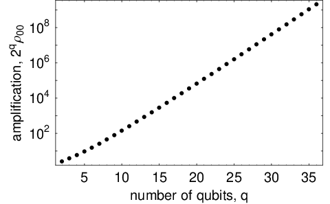
We now investigate the weak decay limit in some more detail. We choose, somewhat arbitrarily, as representative of this low- limit. The steady state population of the solution, , is then much larger than the other populations. We also see that decreases with increasing . A plot of vs. is remarkably well fitted by a straight line. However this relationship is purely heuristical and extrapolates to negative population for .
We define as an “amplification factor”, i.e. the factor by which is increased compared to the fully random case. This is also the ratio of the values in the low- and the high- limits. In Fig. 3 we show how the amplification varies with in an approximately exponential fashion.
It is interesting to compare the weak decay case to a strongly driven two-level system with spontaneous emission. The populations of the ground and excited states then both approach the value 1/2. In the quantum search the population is generally much smaller, except for very small numbers of qubits. However, if we project the numerically obtained steady state on the subspace spanned by , we do find equal populations in these two states.

The observation that becomes ever smaller for larger numbers of qubits may seem disappointing at first. However this is unjustly so. We now investigate how the remaining population is distributed and show that it is concentrated in states at small Hamming distance from the solution.
The diagonal elements of the density matrix are retrieved as . Sorting these by their Hamming distance , and multiplying by their multiplicity (a binomial coefficient), we obtain the distribution of population over the Hamming distance to the solution. This is shown in Fig. 4. For small numbers of qubits the distribution is peaked at . For larger the peak shifts away from zero. This can be understood qualitatively because the multiplicity increases rapidly with .
For strong decay the mean of the distribution . A readout then yields a wrong bit value for half the bits, on average. For weak decay we find that the “bit error rate” is again almost constant, with a value of , as can be seen in Fig. 4. The solution can now be obtained by repeating the search a limited number of times using a majority vote rule to decide about each individual bit value. We can estimate how many times we must repeat the search and readout in order to increase the probability to find an error-free solution to above a preset probability.
The probability that the majority vote yields the wrong result for a particular bit is obtained by summing the binomial distribution, , for (for odd ). For large we can approximate the summation using standard techniques and obtain an upper bound for the single-bit error rate after majority voting,
| (13) |
The probability of an error in at least one bit out of is then given by . For and we find that for .
It is important to note the scaling behavior of . From Eq. (13) we see that decreases faster than exponential with . Thus, if we demand that drops below some preset error probability , the number of repetitions will increase only as . The total search time then scales as , somewhat longer than for the commonly studied relaxation-free case () but still much shorter than for a classical search ().
V Conclusion
In conclusion, we have shown that a modified, robust version of Grover’s quantum search algorithm can be used if the qubits are subject to spontaneous decay. The search is conducted in a Hadamard transformed basis and the single-qubit decay rate must be smaller than the natural oscillation frequency of the search algorithm.
A symmetry allowed us to numerically analyze the problem for up to 36 qubits on a standard desktop computer. This clearly opens up the possibility to investigate this problem for even larger number of qubits, at only polynomial costs. It remains an open question what will happen to the observed constant bit error rate of 0.28 and the trend in the limit . The latter must break down at around 100 qubits. Possibly, an analytic approximation in this limit could shed light on this issue.
An obvious extension of the present work is multiple-item searching for which we expect similarly robust behavior in the presence of relaxation. We can only speculate on the question whether similar modifications may be applied to other quantum algorithms.
Acknowledgements.
We gratefully acknowledge M. Richter and H.B. van Linden van den Heuvell for sharing computer facilities for the highest results, F. Terra and B. Rem for help in obtaining data. This work is part of the research program of the Stichting voor Fundamenteel Onderzoek van de Materie (Foundation for the Fundamental Research on Matter) and was made possible by financial support from the Nederlandse Organisatie voor Wetenschappelijk Onderzoek (Netherlands Organization for the Advancement of Research).*
Appendix A Re-expression of the master equation
Using the symmetry described above, we relabel the density matrix elements using the bit pair counts, . The master equation can then be re-expressed as follows,
| (14) |
where is the Kronecker delta and and are row and column sums, given by
| (15) |
| (16) |
References
- (1) W. G. Unruh, Phys. Rev. A 51, 992 (1995).
- (2) G. M. Palma, K.-A. Suominen, and A. K. Ekert, Proc. R. Soc. Lond. A 452, 567 (1996).
- (3) C. Miquel, J. P. Paz, and R. Perazzo, Phys. Rev. A 54, 2605 (1996).
- (4) P. W. Shor, Phys. Rev. A 52, R2493 (1995).
- (5) A. M. Steane, Phys. Rev. Lett. 77, 793 (1996).
- (6) M. B. Plenio, S. F. Huelga, A. Beige, and P. L. Knight, Phys. Rev. A 59, 2468 (1999).
- (7) A. Beige et al., J. Mod. Opt. 47, 2583 (2000).
- (8) M. B. Plenio and S. F. Huelga, Phys. Rev. Lett. 88, 197901 (2002).
- (9) L. K. Grover, Phys. Rev. Lett. 79, 325 (1997).
- (10) C. Miquel, J. P. Paz, and W. H. Zurek, Phys. Rev. Lett. 78, 3971 (1997).
- (11) B. Pablo-Norman and M. Ruiz-Altaba, Phys. Rev. A 61, 012301 (1999).
- (12) G. L. Long, Y. S. Li, W. L. Zhang, and C. C. Tu, Phys. Rev. A 61, 042305 (2000).
- (13) P. H. Song and I. Kim, Eur. Phys. J. D 23, 299 (2003).
- (14) S. Bettelli, Phys. Rev. A 69, 042310 (2004).
- (15) O. V. Zhirov and D. L. Shepelyansky, Eur. Phys. J. D 38, 405 (2006).
- (16) T. W. Hijmans, T. N. Huussen, and R. J. C. Spreeuw, J. Opt. Soc. Am. B 24, 214 .
- (17) N. Bhattacharya, H. B. van Linden van den Heuvell, and R. J. C. Spreeuw, Phys. Rev. Lett. 88, 137901 (2002).
- (18) A. M. Childs, E. Farhi, and J. Preskill, Phys. Rev. A 65, 012322 (2001).
- (19) R. P. Feynman, Int. J. of Theor. Phys. 21, 467 (1982).
- (20) E. Farhi and S. Gutmann, Phys. Rev. A 57, 2403 (1998).
- (21) J. Roland and N. J. Cerf, Phys. Rev. A 65, 042308 (2002).
- (22) E. Farhi, J. Goldstone, S. Gutmann, and M. Sipser, quant-ph/0001106 .
- (23) E. Farhi et al., Science 292, 472 (2001).
- (24) P. M. Visser and G. Nienhuis, Phys. Rev. A 52, 4727 (1995).