One-mode Bosonic Gaussian channels: a full weak-degradability classificationThanks: The Leverhulme Visiting Professor at Centre for Quantum Computation, Department of Applied Mathematics and Theoretical Physics, Cambridge University.

Consider a single Bosonic mode characterized by canonical observables $Q_{a},P_{a}$ obeying the canonical commutation relation $[Q_{a},P_{a}]=i$. A consistent description of the system can be given in terms of the unitary Weyl operators $V_{a}(z)=\exp\,[i(Q_{a},P_{a})\cdot z]$, with $z=(x,y)^{T}$ being a column vector of $R^{2}$. In this framework the canonical commutation relation is written as

$$V_{a}(z)\;V_{a}(z^{\prime})=\exp[\frac{i}{2}\Delta(z,z^{\prime})]\;V_{a}(z+z^{\prime})\;,$$

where $\Delta(z,z^{\prime})$ is the symplectic form

$$\Delta(z,z^{\prime})=-i\;z^{T}\cdot\sigma_{2}\cdot z^{\prime}=x^{\prime}y-xy^{\prime}\;,$$

(2.1)

with $\sigma_{2}$ being the second Pauli matrix. Moreover the density operators $\rho_{a}$ of the system can be expressed in terms of an integral over $z$ of the $V_{a}(z)$’s, i.e.

$\displaystyle\rho_{a}=\int\frac{d^{2}z}{2\pi}\;\phi(\rho_{a};z)\;V_{a}(-z)\;,$

(2.2)

with

$\displaystyle\phi(\rho_{a};z)=\mbox{Tr}_{a}[\rho_{a}\;V_{a}(z)]\;,$

(2.3)

being the characteristic function of $\rho_{a}$ ¹¹ 1 In effect an analogous decomposition (2.2) holds also for all trace class operators of $A$ [30].. Consequently a complete description of a quantum channel on $A$ is obtained by specifying its action on the operators $V_{a}(z)$, or, equivalently, by specifying how to construct the characteristic function $\phi(\Phi(\rho_{a});z)$ of the evolved states. In the case of Gaussian channels $\Phi$ this is done by assigning a mapping of the Weyl operators

$$\Phi_{H}(V_{a}(z))=V_{a}(K\cdot z)\;\exp[-\frac{1}{2}\;z^{T}\cdot\alpha\cdot z+i\;m^{T}\cdot z]\;,$$

(2.4)

in the Heisenberg picture, or the transformation of the characteristic functions

$\displaystyle\phi(\Phi(\rho_{a});z)=\phi(\rho_{a};K\cdot z)\;\exp[-\frac{1}{2}\;z^{T}\cdot\alpha\cdot z+i\;m^{T}\cdot z],$

(2.5)

in the Schrödinger picture. Here $m$ is a vector, while $K$ and $\alpha$ are real matrices (the latter being symmetric and positive). Equation (2.5) guarantees that any input Gaussian characteristic function will remain Gaussian under the action of the map. A useful property of Gaussian channels is the fact that the composition of two of them (say $\Phi^{\prime}$ and $\Phi^{\prime\prime}$) is still a Gaussian channel. Indeed one can easily verify that the composite map $\Phi^{\prime\prime}\circ\Phi^{\prime}$ is of the form (2.5) with $m$, $K$ and $\alpha$ given by

	$\displaystyle m$	$\displaystyle=$	$\displaystyle(K^{\prime\prime})^{T}\cdot m^{\prime}+m^{\prime\prime}$
	$\displaystyle K$	$\displaystyle=$	$\displaystyle K^{\prime}\;K^{\prime\prime}$		(2.6)
	$\displaystyle\alpha$	$\displaystyle=$	$\displaystyle(K^{\prime\prime})^{T}\;\alpha^{\prime}\;K^{\prime\prime}+\alpha^{\prime\prime}\;.$

Here $m^{\prime}$, $K^{\prime}$, and $\alpha^{\prime}$ belongs to $\Phi^{\prime}$ while $m^{\prime\prime}$, $K^{\prime\prime}$, and $\alpha^{\prime\prime}$ belongs to $\Phi^{\prime\prime}$.

Not all possible choices of $K$, $\alpha$ correspond to transformations $\Phi$ which are completely positive. A necessary and sufficient condition for this last property (adapted to the case of one mode) is provided by the nonnegative definiteness of the following $2\times 2$ Hermitian matrix [3, 20]

$$2\;\alpha-\sigma_{2}+K^{T}\;\sigma_{2}\;K\;.$$

(2.7)

This matrix reduces to $2\alpha+(\mbox{Det}[K]-1)\;\sigma_{2}$ and its nonnegative definiteness to the inequality

$\displaystyle\mbox{Det}[\alpha]\geqslant\left(\frac{\mbox{Det}[K]-1}{2}\right)^{2}\;.$

(2.8)

Within the limit imposed by Eq. (2.8) we can use Eq. (2.5) to describe the whole set of the one-mode Gaussian channels.

An important subset of one-mode Gaussian channels is given by the maps $\Phi$ which possess a physical representation (1.1) with $\rho_{b}$ being a Gaussian state of a single external Bosonic mode $B$ and with $U_{ab}$ being a canonical transformation of $Q_{a}$, $P_{a}$, $Q_{b}$ and $P_{b}$ (the latter being the canonical observables of the mode $B$). In particular let $\rho_{b}$ be a thermal state of average photon number $N$, i.e.

$\displaystyle\phi(\rho_{b};z)=\mbox{Tr}_{b}[\rho_{b}\;V_{b}(z)]=\exp[-(N+1/2)|z|^{2}/2]\;,$

(2.9)

and let $U_{ab}$ be such that

$\displaystyle U_{ab}^{\dagger}\;(Q_{a},P_{a},Q_{b},P_{b})\;U_{ab}=(Q_{a},P_{a},Q_{b},P_{b})\cdot M\;,$

(2.10)

with $M$ being a $4\times 4$ symplectic matrix of block form

$\displaystyle M\equiv\left(\begin{array}[]{ccc}m_{11}&|&m_{21}\\ \hline\cr m_{12}&|&m_{22}\end{array}\right)\;.$

This yields the following evolution for the characteristic function $\phi(\rho_{a};z)$,

	$\displaystyle\phi(\Phi(\rho_{a});z)$	$\displaystyle=$	$\displaystyle\mbox{Tr}_{a}[\Phi(\rho_{a})\;V_{a}(z)]=\mbox{Tr}_{a}[\rho_{a}\;\Phi_{H}(V_{a}(z))]$		(2.14)
		$\displaystyle=$	$\displaystyle\mbox{Tr}_{ab}\left[U_{ab}^{\dagger}\;(V_{a}(z)\otimes\hbox{\small 1\kern-3.8pt\normalsize 1})U_{ab}\;(\rho_{a}\otimes\rho_{b})\right]$
		$\displaystyle=$	$\displaystyle\mbox{Tr}_{ab}\left[\big(V_{a}(m_{11}\cdot z)\otimes V_{b}(m_{12}\cdot z)\big)\;(\rho_{a}\otimes\rho_{b})\right]$
		$\displaystyle=$	$\displaystyle\phi(\rho_{a};m_{11}\cdot z)\;\exp[-(N+1/2)|m_{12}\cdot z|^{2}/2]\;,$

which is of the form (2.5) by choosing $m=0$, $K=m_{11}$ and $\alpha=(N+1/2)\;m_{12}^{T}\cdot m_{12}$. It is worth stressing that in the case of Eq. (2.14) the inequality (2.8) is guaranteed by the symplectic nature of the matrix $M$, i.e. by the fact that Eq. (2.10) preserves the commutation relations among the canonical operators. Indeed we have

	$\displaystyle\mbox{Det}[\alpha]$	$\displaystyle=$	$\displaystyle(N+1/2)^{2}\;\mbox{Det}[m_{12}]^{2}=(N+1/2)^{2}\;(\mbox{Det}[m_{11}]-1)^{2}$		(2.15)
		$\displaystyle\geqslant$	$\displaystyle(\mbox{Det}[K]-1)^{2}/4\;,$

where in the second identity the condition (2.38) was used.

As we shall see, with certain important exception one-mode Gaussian channels (2.4) are unitarily equivalent to transformations which admit physical representation with $\rho_{b}$ and $U_{ab}$ as in Eqs. (2.9) and (2.10).

Following Ref. [20] any Gaussian channel (2.5) can be transformed (through unitarily equivalence) into a simple canonical form. Namely, given a channel $\Phi$ characterized by the vector $m$ and the matrices $K$, $\alpha$ of Eq. (2.5), one can find unitary operators $U_{a}$ and $W_{a}$ such that the channel defined by the mapping

$\displaystyle\rho_{a}\longrightarrow\Phi^{(\text{can})}(\rho_{a})=W_{a}\;\Phi(U_{a}\;\rho_{a}\;U_{a}^{\dagger})\;W_{a}^{\dagger}\qquad\quad\mbox{for all $\rho_{a}$,}$

(2.16)

is of the form (2.5) with $m=0$ and with $K$, $\alpha$ replaced, respectively, by the matrices $K_{\text{can}}$, $\alpha_{\text{can}}$ of Table 1, i.e.

$\displaystyle\phi(\Phi^{(\text{can})}(\rho_{a});z)=\phi(\rho_{a};K_{\text{can}}\cdot z)\;\exp[-\frac{1}{2}\;z^{T}\cdot\alpha_{\text{can}}\cdot z]\;.$

(2.17)

An important consequence of Eq. (2.17) is that to analyze the weak-degradability properties of a one-mode Gaussian channel it is sufficient to focus on the canonical map $\Phi^{(\text{can})}$ which is unitarily equivalent to it (see remark at the end of Sec. 1). Here we will not enter into the details of the derivation of Eqs. (2.16) and (2.17), see Ref. [20].

The dependence on the matrix $K_{\text{can}}$ of $\Phi^{(\text{can})}$ upon the parameters of $\Phi$ can be summarized as follows,

$\displaystyle K_{\text{can}}=\left\{\begin{array}[]{cll}\left\{\begin{array}[]{lll}\sqrt{\mbox{Det}[K]}\;\hbox{\small 1\kern-3.8pt\normalsize 1}&&\mbox{Det}[K]\geqslant 0\\ \sqrt{|\mbox{Det}[K]|}\;\sigma_{3}&&\mbox{Det}[K]<0\end{array}\right.&&\mbox{rank}[K]\neq 1\\ \\ (\hbox{\small 1\kern-3.8pt\normalsize 1}+\sigma_{3})/2&&\mbox{rank}[K]=1\;,\end{array}\right.$

with $\sigma_{3}$ being the third Pauli matrix. Analogously for $\alpha_{\text{can}}$ we have

$\displaystyle\alpha_{\text{can}}=\left\{\begin{array}[]{cll}\sqrt{\mbox{Det}[\alpha]}\;\hbox{\small 1\kern-3.8pt\normalsize 1}&&\mbox{rank}[\alpha]\neq 1\\ \\ \;N_{c}\;(\hbox{\small 1\kern-3.8pt\normalsize 1}-\sigma_{3})/2&&\mbox{rank}[\alpha]=1\;.\end{array}\right.$

The quantity $N_{c}$ is a free parameter which can set to any positive value upon properly calibrating the unitaries $U_{a}$ and $W_{a}$ of Eq. (2.16). Following Ref. [20] we will assume $N_{c}=1/2$. Notice also that from Eq. (2.8), $\mbox{rank}[\alpha]=1$ is only possible for $\mbox{Det}[K]=1$.

Equations (2.3) and (2.3) show that only the determinant and the rank of $K$ and $\alpha$ are relevant for defining $K_{\text{can}}$ and $\alpha_{\text{can}}$. Indeed one can verify that $K_{\text{can}}$ and $\alpha_{\text{can}}$ maintain the same determinant and rank of the original matrices $K$ and $\alpha$, respectively. This is a consequence of the fact the $\Phi$ and $\Phi^{(\text{can})}$ are connected through a symplectic transformation for which $\mbox{Det}[K]$, $\mbox{Det}[\alpha]$, $\mbox{rank}[K]$, and $\mbox{rank}[\alpha]$ are invariant quantities. [In particular $\mbox{Det}[K]$ is directly related with the invariant quantity $q$ analyzed in Ref. [19].]

The six inequivalent canonical forms of Table 1 follow by parametrizing the value of $\sqrt{\mbox{Det}[\alpha]}$ to account for the constraints imposed by the inequality (2.8). It should be noticed that to determine which class a certain channel belongs to, it is only necessary to know if $\mbox{Det}[K]$ is null, equal to $1$, negative or positive ($\neq 1$). If $\mbox{Det}[K]=0$ the class is determined by the rank of the matrix. If $\mbox{Det}[K]=1$ the class is determined by the rank of $\alpha$ (see Fig. 1). Within the various classes, the specific expression of the canonical form depends then upon the effective values of $\mbox{Det}[K]$ and $\mbox{Det}[\alpha]$. We observe also that the class $A_{1}$ can be obtained as a limiting case (for $\kappa\rightarrow 0$) of the maps of class $C$ or $D$. Analogously the class $B_{2}$ can be obtained as a limiting case of the maps of class $C$. Indeed consider the channel with $K_{\text{can}}=\kappa\hbox{\small 1\kern-3.8pt\normalsize 1}$ and $\alpha_{\text{can}}=|\kappa^{2}-1|(N_{0}^{\prime}+1/2)\hbox{\small 1\kern-3.8pt\normalsize 1}$ with $N_{0}^{\prime}={N_{0}}/({|\kappa^{2}-1|})-1/2$, with $N_{0}$ and $\kappa$ positive ($\kappa\neq 0,1$). For $\kappa$ sufficiently close to $1$, $N_{0}^{\prime}$ is positive and the maps belongs to the class $C$ of Table 1. Moreover in the limit of $\kappa\rightarrow 1$ this channel yields the map $B_{2}$.

Finally it is interesting to study how the canonical forms of Table 1 compose under the product (2.6). A simple calculation shows that the following rules apply

$\displaystyle\begin{array}[]{c|cccccc}\circ&A_{1}&A_{2}&B_{1}&B_{2}&C&D\\ \hline\cr A_{1}&A_{1}&A_{1}&A_{1}&A_{1}&A_{1}&A_{1}\\ A_{2}&A_{1}&A_{2}&A_{2}&A_{2}&A_{2}&A_{2}\\ B_{1}&A_{1}&A_{2}&B_{1}&B_{1}/B_{2}&C&D\\ B_{2}&A_{1}&A_{2}&B_{1}/B_{2}&B_{2}&C&D\\ C&A_{1}&A_{2}&C&C&B_{2}/C&D\\ D&A_{1}&A_{2}&D&D&D&C\end{array}$

In this table, for instance, the element on the row 2 and column 3 represents class (i.e. $A_{2}$) associated to the product $\Phi^{\prime\prime}\circ\Phi^{\prime}$ between a channel $\Phi^{\prime}$ of $B_{1}$ and a channel $\Phi^{\prime\prime}$ of $A_{2}$. Notice that the canonical form of the products $B_{1}\circ B_{2}$, $B_{2}\circ B_{1}$ and $C\circ C$ is not uniquely defined. In the first case in fact, even though the determinant of the matrix $K$ of Eq. (2.6) is one, the rank of the corresponding $\alpha$ might be one or different from one depending on the parameters of the two “factor” channels: consequently the $B_{1}\circ B_{2}$ and $B_{2}\circ B_{1}$ might belong either to $B_{1}$ or to $B_{2}$. In the case of $C\circ C$ instead it is possible that the resulting channel will have $\mbox{Det}[K]=1$ making it a $B_{2}$ map. Typically however $C\circ C$ will be a map of $C$. Composition rules analogous to those reported here have been extensively analyzed in Refs. [19, 16, 17].

Apart from the case $B_{2}$ that will be treated separately (see next section), all canonical transformations of Table 1 can be expressed as in Eq. (2.14), i.e. through a physical representation (1.1) with $\rho_{b}$ being a thermal state (2.9) of a single external Bosonic mode $B$ and $U_{ab}$ being a linear transformation (2.10)²² 2 The exceptional role of $B_{2}$ corresponds to the fact that any one-mode Bosonic Gaussian channel can be represented as a unitary coupling with a single-mode environment plus an additive classical noise (see next section and Ref. [4]).. To show this it is sufficient to verify that, for each of the classes of Table 1 but $B_{2}$, there exists a non-negative number $N$ and a symplectic matrix $M$ such that Eq. (2.14) gives the mapping (2.17). This yields the conditions

	$\displaystyle m_{11}$	$\displaystyle=$	$\displaystyle K_{\text{can}}\;,$		(2.36)
	$\displaystyle m_{12}$	$\displaystyle=$	$\displaystyle O\;\sqrt{\frac{\alpha_{\text{can}}}{N+1/2}}\;,$		(2.37)

with $O^{T}=O^{-1}$ being an orthogonal $2\times 2$ matrix to be determined through the symplectic condition

$\displaystyle\mbox{Det}[m_{11}]+\mbox{Det}[m_{12}]=1\;,$

(2.38)

which guarantees that $U_{ab}^{\dagger}Q_{a}U_{ab}$ and $U_{ab}^{\dagger}P_{a}U_{ab}$ satisfy canonical commutation relations. It is worth noticing that once $m_{11}$ and $m_{12}$ are determined within the constraint (2.38) the remaining blocks (i.e. $m_{21}$ and $m_{22}$) can always be found in order to satisfy the remaining symplectic conditions of $M$. An explicit example will be provided in few paragraphs. For the classes $A_{1}$, $A_{2}$, $B_{1}$, $D$, and $C$ with $\kappa<1$, Eqs. (2.37) and (2.38) can be solved by choosing $O=\hbox{\small 1\kern-3.8pt\normalsize 1}$ and $N=N_{0}$. Indeed for $B_{1}$ the latter setting is not necessary. Any non-negative number will do the job: thus we choose $N=0$ making the density matrix $\rho_{b}$ of Eq. (2.9) the vacuum of the $B$. For $C$ with $\kappa>1$ instead a solution is obtained by choosing $O=\sigma_{3}$ and again $N=N_{0}$. The corresponding transformations (2.10) for $Q_{a}$ and $P_{a}$ (together with the choice for $N$) are summarized below.

$\displaystyle\begin{array}[]{cc|c|ccc}\mbox{Class}&&\rho_{b}&U_{ab}^{\dagger}\;Q_{a}\;U_{ab}&&U_{ab}^{\dagger}\;P_{a}\;U_{ab}\\ \hline\cr A_{1}&&\mbox{thermal}(N=N_{0})&Q_{b}&&P_{b}\\ A_{2}&&\mbox{thermal}(N=N_{0})&Q_{a}+Q_{b}&&P_{b}\\ B_{1}&&\mbox{vacuum}(N=0)&Q_{a}&&P_{a}+P_{b}\\ C&\kappa<1&\mbox{thermal}(N=N_{0})&\kappa\;Q_{a}+\sqrt{1-\kappa^{2}}\;Q_{b}&&\kappa\;P_{a}+\sqrt{1-\kappa^{2}}\;P_{b}\\ C&\kappa>1&\mbox{thermal}(N=N_{0})&\kappa\;Q_{a}+\sqrt{\kappa^{2}-1}\;Q_{b}&&\kappa\;P_{a}-\sqrt{\kappa^{2}-1}\;P_{b}\\ D&&\mbox{thermal}(N=N_{0})&{\kappa}\;Q_{a}+\sqrt{\kappa^{2}+1}\;Q_{b}&&-{\kappa}\;P_{a}+\sqrt{\kappa^{2}+1}\;P_{b}\;.\end{array}$

To complete the definition of the unitary operators $U_{ab}$ we need to provide also the transformations of $Q_{b}$ and $P_{b}$. This corresponds to fixing the blocks $m_{21}$ and $m_{22}$ of $M$ and cannot be done uniquely: one possible choice is presented in the following table

$\displaystyle\begin{array}[]{cc|ccc}\mbox{Class}&&U_{ab}^{\dagger}\;Q_{b}\;U_{ab}&&U_{ab}^{\dagger}\;P_{b}\;U_{ab}\\ \hline\cr A_{1}&&Q_{a}&&P_{a}\\ A_{2}&&Q_{a}&&P_{a}-P_{b}\\ B_{1}&&Q_{a}-Q_{b}&&-P_{b}\\ C&\kappa<1&\sqrt{1-\kappa^{2}}\;Q_{a}-\kappa\;Q_{b}&&\sqrt{1-\kappa^{2}}\;P_{a}-\kappa\;P_{b}\\ C&\kappa>1&\sqrt{\kappa^{2}-1}\;Q_{a}+\kappa\;Q_{b}&&-\sqrt{\kappa^{2}-1}\;P_{a}+\kappa\;P_{b}\\ D&&\sqrt{\kappa^{2}+1}\;Q_{a}+{\kappa}\;Q_{b}&&\;\sqrt{\kappa^{2}+1}\;P_{a}-{\kappa}\;P_{b}\;.\end{array}$

The above definitions make explicit the fact that the canonical form $C$ represents attenuator ($\kappa<1$) and amplifier ($\kappa>1$) channel [3]. We will see in the following sections that the class $D$ is formed by the weakly complementary of the amplifier channels of the class $C$. For the sake of clarity the explicit expression for the matrices $M$ of the various classes has been reported in App. A.

Finally it is important to notice that the above physical representations are equivalent to Stinespring representations only when the average photon number $N$ of $\rho_{b}$ nullifies. In this case the environment $B$ is represented by a pure input state (i.e. the vacuum). According to our definitions this is always the case for the canonical form $B_{1}$ while for the canonical forms $A_{1}$, $A_{2}$, $C$ and $D$ it happens for $N_{0}=0$.

As mentioned in the previous section the class $B_{2}$ of Table 1 must be treated separately. The map $B_{2}$ corresponds³³ 3 This can be seen for instance by evaluating the characteristic function of the state (2.54) and comparing it with Eq. (2.17). to the additive classical noise channel [3] defined by

$\displaystyle\Phi(\rho_{a})=\int d^{2}z\;p(z)\;V_{a}(z)\;\rho_{a}\;V_{a}(-z)\;,$

(2.54)

with $p(z)=(2\pi N_{0})^{-1}\;\exp[-|z|^{2}/(2N_{0})]$ which, in Heisenberg picture, can be seen as a random shift of the annihilation operator $a$.

These channels admit a natural physical representation which involve two environmental modes in a pure state (see Ref. [20] for details) but do not have a physical representations (1.1) involving a single environmental mode. This can be verified by noticing that in this case, from Eqs. (2.36) and (2.37) we get

	$\displaystyle m_{11}$	$\displaystyle=$	11		(2.55)
	$\displaystyle m_{12}$	$\displaystyle=$	$\displaystyle\sqrt{N_{0}/(N+1/2)}\;O\;,$		(2.56)

which yields

$\displaystyle\mbox{Det}[m_{11}]+\mbox{Det}[m_{12}]=1\pm N_{0}/(N+1/2)\;,$

(2.57)

independently of the choice of the orthogonal matrix $O$⁴⁴ 4 This follows from the fact that $\mbox{Det}[O]=\pm 1$ since $O^{T}=O^{-1}$.. Therefore, apart from the trivial case $N_{0}=0$, the only solution to the constraint (2.38) is by taking the limit $N\rightarrow\infty$. This would correspond to representing the channel $B_{2}$ in terms of a linear coupling with a single-mode thermal state $\rho_{b}$ of “infinite” temperature. Unfortunately this is not a well defined object. However we can use the “asymptotic” representation described at the end of Sec. 2.3 where it was shown how to obtain $B_{2}$ as limiting case of $C$ class maps, to claim at least that there exists a one-parameter family of one-mode Gaussian channels which admits single-mode physical representation and which converges to $B_{2}$.

In this section we construct the weakly complementary channels $\tilde{\Phi}$ of the class $A_{1}$, $A_{2}$, $B_{1}$, $C$ and $D$ starting from their single-mode physical representations (1.1) of Sec. 2.4. Because of the linearity of $U_{ab}$ and the fact that $\rho_{b}$ is Gaussian, the channels $\tilde{\Phi}$ are Gaussian. This can be seen for instance by computing the characteristic function (2.3) of the output state $\tilde{\Phi}(\rho_{a})$

	$\displaystyle\phi(\tilde{\Phi}(\rho_{a});z)$	$\displaystyle=$	$\displaystyle\mbox{Tr}_{b}[\tilde{\Phi}(\rho_{a})\;V_{b}(z)]=\mbox{Tr}_{b}[\rho_{a}\;\tilde{\Phi}_{H}(V_{b}(z))]$		(3.1)
		$\displaystyle=$	$\displaystyle\phi(\rho_{a};m_{21}\cdot z)\;\exp[-\frac{1}{2}(N+1/2)\;|m_{22}\cdot z|^{2}]\;,$

where $m_{21}$, $m_{22}$ are the blocks elements of the matrix $M$ of Eq. (2.2) associated with the transformations $U_{ab}$, and with $N$ being the average photon number of $\rho_{b}$ (the values of these quantities are given in the tables of Sec. 2.4 — see also App. A). By setting $m=0$, $K=m_{21}$ and $\alpha=(N+1/2)\;m_{22}^{T}\;m_{22}$, Eq. (3.1) has the same structure (2.5) of the one-mode Gaussian channel of $A$. Therefore by cascading $\tilde{\Phi}$ with an isometry which exchanges $A$ with $B$ (see Refs. [31, 19]) we can then treat $\tilde{\Phi}$ as an one-mode Gaussian channel operating on $A$ (this is possible because both $A$ and $B$ are Bosonic one-mode systems). With the help of Table 1 we can then determine which classes can be associated with the transformation (3.1). This is summarized in Table 2.

Using the compositions rules of Eqs. (2.6) and (2.3) it is easy to verify that the canonical forms $A_{1}$, $A_{2}$, $D$ and $C$ with $\kappa\leqslant\sqrt{1/2}$ are anti-degradable (1.10). Vice-versa one can verify that the canonical forms $B_{1}$ and $C$ with $\kappa\geqslant\sqrt{1/2}$ are weakly degradable (1.9) — for $C$, $D$ and $A_{1}$ these results have been proved in Ref. [19]. Through unitary equivalence this can be summarized by saying that all one-mode Gaussian channels (2.5) having $\mbox{Det}[K]\leqslant 1/2$ are anti-degradable, while the others (with the exception of the channels belonging to $B_{2}$) are weakly degradable (see Fig. 2).

In the following we verify the above relations by explicitly constructing the connecting channels $\Psi$ and $\overline{\Psi}$ of Eqs. (1.9) and (1.10) for each of the mentioned canonical forms. Indeed one has:

• •

  For a channel $\Phi$ of standard form $A_{1}$ or $A_{2}$, anti-degradability can be shown by simply taking $\overline{\Psi}$ of Eq. (1.10) coincident with the channel $\Phi$. The result immediately follows from the composition rule (2.6).

• •

  For a channel $\Phi$ of $B_{1}$, weak-degradability comes by assuming the map $\Psi$ to be equal to the weakly complementary channel $\tilde{\Phi}$ of $\Phi$ (see Table 2). As pointed out in Ref. [20] this also implies the degradability of $\Phi$ in the sense of Ref. [22]. Let us remind that for $B_{1}$ the physical representation given in Sec. 2.4 was constructed with an environmental state $\rho_{b}$ initially prepared in the vacuum state, which is pure. Therefore in this case our representation gives rise to a Stinespring dilation.

• •

  For a channel $\Phi$ of the class $C$ with $K_{\text{can}}=\kappa\;\hbox{\small 1\kern-3.8pt\normalsize 1}$ and $\alpha_{\text{can}}=|\kappa^{2}-1|(N_{0}+1/2)\hbox{\small 1\kern-3.8pt\normalsize 1}$ we have the following three possibilities:

  • –

    If $\kappa\leqslant\sqrt{1/2}$ the channel is anti-degradable and the connecting map $\overline{\Psi}$ is a channel of $C$ characterized by $K_{\text{can}}=\kappa^{\prime}\;\hbox{\small 1\kern-3.8pt\normalsize 1}$ and $\alpha_{\text{can}}=(1-(\kappa^{\prime})^{2})(N_{0}+1/2)\hbox{\small 1\kern-3.8pt\normalsize 1}$ with $\kappa^{\prime}=\kappa/\sqrt{1-\kappa^{2}}<1$.

  • –

    If $\kappa\in[\sqrt{1/2},1[$ the channel is weakly degradable and the connecting map ${\Psi}$ is again a channel of $C$ defined as in the previous case but with $\kappa^{\prime}=\sqrt{1-\kappa^{2}}/\kappa<1$. For $N_{0}=0$ the channel is also degradable [22] since our physical representation is equivalent to a Stinespring representation.

  • –

    If $\kappa>1$ the channel is weakly degradable and the connecting map ${\Psi}$ is a channel of $D$ with $K_{\text{can}}=\kappa^{\prime}\;\hbox{\small 1\kern-3.8pt\normalsize 1}$ and $\alpha_{\text{can}}=((\kappa^{\prime})^{2}-1)(N_{0}+1/2)\hbox{\small 1\kern-3.8pt\normalsize 1}$ with $\kappa^{\prime}=\sqrt{k^{2}-1}/k$. As in the previous case, for $N_{0}=0$ the channel is also degradable [22].

• •

  For a channel $\Phi$ of $D$ with $K_{\text{can}}=\kappa\;\sigma_{3}$ and $\alpha_{\text{can}}=(\kappa^{2}+1)(N_{0}+1/2)\hbox{\small 1\kern-3.8pt\normalsize 1}$ ($\kappa>0$ and $N_{0}\geqslant 0$) we can prove anti-degradability by choosing $\overline{\Psi}$ of Eq. (1.10) to be yet another maps of $D$ with $K_{\text{can}}=\kappa^{\prime}\;\sigma_{3}$ and $\alpha_{\text{can}}=((\kappa^{\prime})^{2}+1)(N_{0}+1/2)\hbox{\small 1\kern-3.8pt\normalsize 1}$ where $\kappa^{\prime}=\kappa/\sqrt{\kappa^{2}+1}$. From Eq. (2.6) and Table 2 it then follows that $\Psi\circ\tilde{\Phi}$ is indeed equal to $\Phi$.

Concerning the case $B_{2}$ it was shown in Ref. [20] that the channel is neither anti-degradable nor degradable in the sense of [22] (apart from the trivial case $N_{0}=0$ which corresponds to the identity map). On the other hand one can use the continuity argument given in Sec. 2.5 to claim that the channel $B_{2}$ can be arbitrarily approximated with maps which are weakly degradable (those belonging to $C$ for instance).

We observe that according to composition rule (2.3) the combination of any two channels $\Phi_{1}$ and $\Phi_{2}$ of $D$ produces a map $\Phi_{21}\equiv\Phi_{2}\circ\Phi_{1}$ which is in the class $C$. Since the class $D$ is anti-degradable the resulting channel must have null quantum capacity. Let then $\kappa_{j}\sigma_{3}$ and $(\kappa^{2}_{j}+1)(N_{j}+1/2)\hbox{\small 1\kern-3.8pt\normalsize 1}$ be the matrices $K_{\text{can}}$ and $\alpha_{\text{can}}$ of the channels $\Phi_{j}$, for $j=1,2$. From Eq. (2.6) one can then verify that $\Phi_{21}$ has the canonical form $C$ with parameters

	$\displaystyle\kappa$	$\displaystyle=$	$\displaystyle\kappa_{1}\kappa_{2}\;,$		(4.1)
	$\displaystyle N_{0}$	$\displaystyle=$	$\displaystyle\frac{(\kappa_{2}^{2}+1)N_{2}+\kappa_{2}^{2}(\kappa_{1}^{2}+1)N_{1}}{|\kappa_{1}^{2}\kappa_{2}^{2}-1|}+\frac{1}{2}\left(\frac{\kappa^{2}_{1}\kappa_{2}^{2}+2\kappa_{2}^{2}+1}{|\kappa_{1}^{2}\kappa_{2}^{2}-1|}-1\right)\;.$		(4.2)

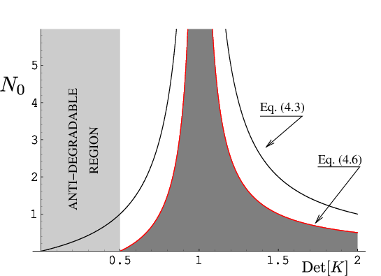
Equation (4.1) shows that by varying $\kappa_{j}$, $\kappa$ can take any positive values: in particular it can be greater than $\sqrt{1/2}$ transforming $\Phi_{21}$ into a channel which does not belong to the anti-degradable area of Fig. 2. On the other hand, by varying the $N_{j}$ and $\kappa_{2}$, but keeping the product $\kappa_{1}\kappa_{2}$ fixed, the parameter $N_{0}$ can assume any value satisfying the inequality

$\displaystyle N_{0}$

$\displaystyle\geqslant$

$\displaystyle\frac{1}{2}\left(\frac{\kappa^{2}+1}{|\kappa^{2}-1|}-1\right)\;.$

(4.3)

We can therefore conclude that all channels $C$ with $\kappa$ and $N_{0}$ as in Eq. (4.3) have null quantum capacity — see Fig. 3. A similar bound was found in a completely different way in Ref. [3].

References

- [1] C. H. Bennett and P. W. Shor, IEEE Trans. Inf. Theory 44, 2724 (1998).
- [2] A. S. Holevo, Probl. Inform. Transm. 8, 63, (1972).
- [3] A. S. Holevo and R. F. Werner, Phys. Rev. A 63 032312 (2001).
- [4] J. Eisert and M. M. Wolf, E-print quant-ph/0505151.
- [5] R. G. Gallager, Information Theory and Realible Communication (Wiley, New York, 1968).
- [6] S. Braunstein and P. van Look, Rev. Mod. Phys. 77, 513 (2005).
- [7] C. M. Caves and P. D. Drummond, Rev. Mod. Phys. 66, 481 (1994); H. P. Yuen and M. Ozawa, Phys. Rev. Lett. 70 363 (1993).
- [8] A. S. Holevo, M. Sohma, and O. Hirota, Phys. Rev. A 59, 1820 (1999).
- [9] V. Giovannetti, S. Guha, S. Lloyd, L. Maccone, J. H. Shapiro, and H. P. Yuen, Phys. Rev. Lett. 92, 027902 (2004).
- [10] V. Giovannetti, S. Lloyd, L. Maccone and P.W. Shor, Phys. Rev. Lett. 91, 047901 (2003); Phys. Rev. A 68, 062323 (2003).
- [11] A. S. Holevo, IEEE Trans. Inf. Theory 44, 269 (1998); P. Hausladen, R. Jozsa, B. Schumacher, M. Westmoreland and W. K. Wootters, Phys. Rev. A 54, 1869 (1996); B. Schumacher and M. D. Westmoreland, Phys. Rev. A 56, 131 (1997).
- [12] A. S. Holevo, Probability Theory and Application, 48, 359 (2003); A. S. Holevo and and M. E. Shirokov, Commun. Math. Phys. 249, 417, 2004; M. E. Shirovov, Commun. Math. Phys. 262, 137 (2006) ; A. S Holevo and M. E. Shirokov, quant-ph/0408176.
- [13] S. Lloyd, Phys. Rev. A 55, 1613 (1997); H. Barnum, M. A. Nielsen, and B. Schumacher, Phys. Rev. A 57, 4153 (1998); I. Devetak, IEEE Trans. Inform. Theory 51, 44 (2005).
- [14] C.H. Bennett, P. W. Shor, J. A. Smolin, and A. V. Thapliyal, IEEE Trans. Inf. Theory 48, 2637 (2002).
- [15] M.J.W. Hall and M.J. O’Rourke, Quantum Opt. 5 161, (1993); M.J.W. Hall, Phys. Rev. A 50, 3295 (1994); J.H. Shapiro, V. Giovannetti, S. Guha, S. Lloyd, L. Maccone, and B.J. Yen AIP Conf. Proc. 734, 15 (2004); M. Sohma and O. Hirota, quant-ph/0105042.
- [16] V. Giovannetti, S. Guha, S. Lloyd, L. Maccone, and J.H. Shapiro, Phys. Rev. A 70, 032315 (2004); V. Giovannetti, S. Lloyd, L. Maccone, J.H. Shapiro, and B.J. Yen, Phys. Rev. A ib. 70 , 022328 (2004).
- [17] V. Giovannetti and S. Lloyd, Phys. Rev. A 69, 062307 (2004).
- [18] A. Serafini, J. Eisert, and M.M. Wolf, Phys. Rev. A 71 012320 (2005).
- [19] F. Caruso and V. Giovannetti, to appear in Phys. Rev. A (2006), E-print quant-ph/0603257.
- [20] A. S. Holevo, E-print quant-ph/0607051.
- [21] M. M. Wolf and D. Peréz-García, E-print quant-ph/0607070.
- [22] I. Devetak and P. W. Shor, Commun. Math. Phys. 256, 287 (2005).
- [23] W. F. Stinespring, Proc. Am. Math. Soc. 6, 211 (1955).
- [24] G. Lindblad, Commun. Math. Phys. 48, 116 (1976).
- [25] A. S. Holevo, E-print quant-ph/0509101.
- [26] C. King, K. Matsumoto, M. Nathanson, and M. B. Ruskai, E-print quant-ph/0509126.
- [27] W. K. Wootters and W. H. Zurek, Nature 299, 802 (1982).
- [28] N. Gisin and S. Massar, Phys. Rev. Lett. 79, 2153 (1997); D. Bruß, D. P. DiVincenzo, A. Ekert, C. A. Fuchs, C. Macchiavello, and J. A. Smolin, Phys. Rev. A 57, 2368 (1998); R. F. Werner, Phys. Rev. A 58, 1827 (1998); V. Büzek, and M. Hillery, Phys. Rev. Lett. 81, 5003 (1998).
- [29] A. Ferraro, S. Olivares, and M. G. A. Paris, Gaussian states in quantum information (Bibliopolis, Napoli, 2005).
- [30] A. S. Holevo, Probabilistic Aspects of Quantum Theory (North-Holland, Amsterdam, 1982).
- [31] V. Giovannetti and R. Fazio, Phys. Rev. A 71, 032314 (2005).