How much entanglement can be generated between two atoms by detecting photons?
Abstract
It is possible to achieve an arbitrary amount of entanglement between two atoms using only spontaneously emitted photons, linear optics, single photon sources and projective measurements. This is in contrast to all current experimental proposals for entangling two atoms, which are fundamentally restricted to one entanglement bit or “ebit”.
pacs
03.67.Mn,32.80.Pj,42.50.CtIn the world of quantum information processing it is widely accepted that, while photons are the ideal candidates for transmitting quantum information, this information is better stored and manipulated using atomic systems. The reason is that, while photons can be moved through long distances with little decoherence, atoms can be easily confined and can preserve quantum information for a long time. Consequently, an ideal design for a quantum network will conceivably be built upon a number of atomic or solid state devices which communicate through photonic quantum channels.
There exist mainly two methods for entangling distant atoms. One is based on emission of photons by the first atom, which afterwards interact with the second atom generating the entanglement Cirac et al. 1997; van Enk et al. 1997; Gheri et al. 1998; Parkins and Kimble 2000; Chan et al. 2002; Chan et al. 2003. The second method relies on detecting the photons emitted by the two atoms with the subsequent entanglement generation due to interference in the measurement process Cabrillo et al. 1999; Bose et al. 1999. Some ingredients of both proposals have been realized experimentally Julsgaard et al. 2001; Kuhn et al. 2002; McKeever et al. 2004; Blinov et al. 2004; Volz et al. 2006; Matsukevich et al. 2006; Beugnon et al. 2006; Maunz et al. 2006; Chou et al. 2005; Darquie et al. 2005. Most of the experiments with isolated atoms and light aim at entangling the internal state of the atom with the polarization of the photon Kuhn et al. 2002; McKeever et al. 2004; Blinov et al. 2004; Volz et al. 2006; Matsukevich et al. 2006; Beugnon et al. 2006; Maunz et al. 2006; Darquie et al. 2005. It is clear that due to the size of the Hilbert space, the maximum attainable entanglement is one ebit.
In this letter we will deal with the generation of entanglement between two atoms. We will focus on the second method mentioned above, in which entanglement is generated by measurements. To avoid the limit of one ebit, we work with continuous variables and seek entanglement in the motional state of the atoms. We will answer two fundamental questions: How much entanglement can be produced between the atoms? How can we achieve it?
Our first result is that by usual means —two atoms, one or two emitted photons, linear optics and postselection Cabrillo et al. 1999; Maunz et al. 2006—, we cannot produce more than 1 ebit of entanglement between the atoms, even if our Hilbert space is larger. Our second result si that we can achieve an arbitrary amount of entanglement using at least two emitted photons and what we call an Entangling Two-Photon Detector (ETPD). The ETPD is a device which combines both photons in a projective measurement onto a highly entangled state. Note that this approach differs from recent work on entangling Gaussian modes of the quantum electromagnetic field by means of a Kerr medium Kowalewska-Kudlaszyk and Leonski 2006; Olsen 2006. Theoretically, an ETPD could be built using a Kerr medium and postselection, but current nonlinear materials are too inefficient for such implementation 11 1 State of the art down-conversion experiments Volz et al. 2001 achieve an efficiency of for weak laser sources. We expect a much lower efficiency for up-conversion due to having much less photons and the difficulties of mode matching.. Inspired by the KLM proposal Knill et al. 2001, in the last part of our paper we demonstrate an efficient scheme for simulating the ETPD using ancillary photons. Our last result is that introducing additional photons in our setup, together with single-photon detectors, beam-splitters and an attenuator, we can obtain an amount of entanglement of ebits. Finally, at the end of the paper we discuss the relevance of these results and possible implementations.
We have in mind the setup in Ref. Cabrillo et al. 1999 where two atoms, initially at zero–momentum state, are excited with a very small probability. We consider the state of the atoms after spontaneous emission, when both are in the ground state. The state of the system at the end is given by
| (1) | |||||
Here , , denote the momenta of the emitted photons; their associated creation operators and the vacuum state of the EM field, and are the excitation probabilities of the atoms. The initial momentum distribution of the emitted photons is given by for the -th atom. As we will see later, we require some uncertainty in the initial momentum in order to generate a large amount of entanglement. Finally , and denote the recoil momenta of the atoms after emitting the photons. The terms omitted in Eq. (1) correspond to higher order processes where an atom emits more than one photon. These terms will have a very small contribution if the decay time of the atom is longer than the duration of the exciting pulse.
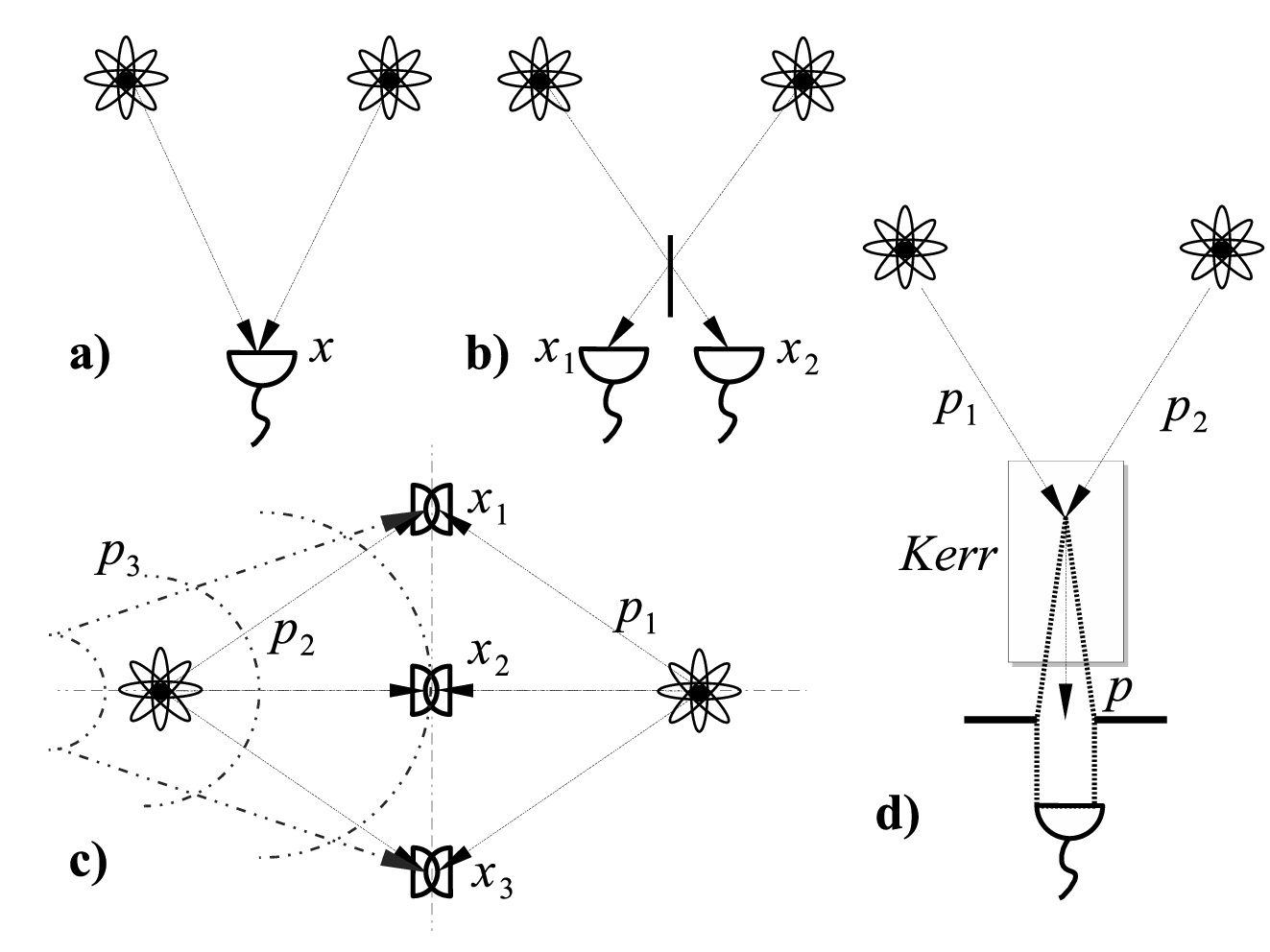
Let us now consider a single detector placed symmetrically below the atoms Cabrillo et al. 1999, as in Fig. 1a. If there is one single photon detection, this will amount to a projective measurement onto a single-photon state and out of the state in Eq. (1) only the term on the first row will survive. Since the photons coming from the atoms are indistinguishable, an implicit symmetrization will take place and the final state of the atoms will be of the form , for some motional states and . Even though we work with continuous variables, this state can have at most 1 ebit which corresponds to .
We are going to show now that with two emitted photons, linear optics and two detectors, we cannot do better than one ebit of entanglement [See Fig. 1b]. The proof generalizes the previous argument with a little bit more care. First of all, linear optics amounts to a linear transformation of the initial momentum modes, , to new operators, . A trivial example of this is a beam splitter, which changes the photons from incident states and to . Linear optics can be combined with measurements. Without loss of generality, all measurements will take place at the end of the process and they amount to a projection onto the modes and for the first and second detector, respectively. The state after a projective measurement onto two single-photon detectors reads
| (2) | |||||
Note that the modes and detected by the first and second detector are expressed on an orthonormal basis different from that of the or operators. We enclose this information, plus the initial wavefunction of the photon in the following -numbers
| (3) |
Using these wavefunctions we define the motional states
| (4) |
The expectation value in Eq. (2) can be written in terms of the . We thus arrive to the following expression for the atomic state after the measurement
| (5) |
This state cannot have more than 1 ebit of entanglement, which happens when all the states , , and are orthogonal to each other.
We must make several remarks. First of all, adding more detectors does not improve the outcome. Second, our proof is valid independently of the number of beam splitters, prisms, lenses and even polarizers we use. In particular, attenuating elements such as polarizers and filters can be treated as a linear operation plus a measurement and are covered by the previous formalism.
We propose now to use an ETPD to obtain an arbitrary degree of entanglement between the two atoms. An ETPD is by definition a device that clicks whenever two photons arrive simultaneously and with their momenta satisfying a certain constraint. An example would be a parametric up-conversion crystal, in which pairs of photons with momenta and are converted with a certain probability into a new photon with momentum . One imposes a constraint on the initial state by post-selecting a window of final momenta. For example, restricting the measurement to photons with transverse momentum , then the initial contributing momenta must be those satisfying [Fig. 1d]. In this example the ETPD ideally projects the initial two photon product state onto the probably entangled state
| (6) |
Here is the acceptance function of the detector or, equivalently, the constraint that the final detected momenta and obey.
We claim now that with two emitted photons, linear operations and an ETPD, there is no limit to the attainable entanglement. To prove it we consider that after projection of the photon part of state in Eq. (1) into , the resulting atomic state will take the form
| (7) |
with the already entangled state
| (8) | |||||
Depending on the specific shape of the functions and , , the corresponding state may reach an unbounded degree of entanglement. For example, let us consider that the photons evolve freely in space without any linear optics elements, , and assume that the detector has a very narrow acceptance function . The wider the initial momentum widths of the two photons, the larger the resulting bipartite atomic entanglement, because a higher uncertainty in the wave packets allows for higher nonlocal correlations, which are not bounded from above. Indeed, in this ideal case the outcome will be much like the EPR pairs from the seminal paper Ref. Einstein et al. 1935.
Current Kerr media are too inefficient to practically implement the ETPD introduced here. Motivated by this we have designed another protocol that simulates the outcome of an ETPD using linear optics, additional photons and postselection. As shown in the KLM proposal Knill et al. 2001, any highly entangling quantum gate can be performed this way, though a lot of care is needed to reduce the number of gates. Our proposal starts up from the two atoms after having emitted two photons which are combined with additional ancillary photons,
| (9) | |||||
The resulting state after linear operations on the photons, and -fold coincidence count on the detectors, will be, analogously to the two-photon and two-detector case [Eqs. (2)-(5)]
| (10) |
where denotes the set of permutations of elements. This state may contain much more than one ebit of entanglement. In fact, an upper bound to the degree of attainable entanglement is ebits. We will show afterwards that this bound is indeed saturated.

As a clarifying example we consider the setup in Fig. 1c with three photons and three detectors. Photons and come from their respective atoms, we introduce a single auxiliary photon, and we place three detectors symmetrically to the atoms, , , . The final state for the two atoms, considering that all the three detectors are excited by the three photons, and fixing relative phases equal to 1 for simplicity purposes, will be
| (11) | |||||
where we denote with the atomic state associated to detection of in , and in . In Fig. 2 we show the processes that contribute coherently to the two-atom final entangled state. This procedure gives an entanglement of ebits.

The previous example is suboptimal. The maximal amount of entanglement of ebits is reachable for some of the states in Eq. (10). To prove it we consider a very symmetric configuration in which the detectors are located along a circle, equidistant to both atoms [Fig. 1c]. We will assume for simplicity that the two emitted photons and the ancillary ones are in -wave states and arrive with equal probability and phase to every detector. In a similar fashion as in Eq. (11), the final bipartite atomic state will take the form
| (12) |
where is the final bipartite atomic state after detection of photon in detector , and photon in detector . In matrix form, the coefficients are
| (13) |
where . Both the reduced density matrix of one atom and the Schmidt rank can be obtained from this matrix. The previous state can be rewritten in the form
| (14) |
where , is a completion of to an orthonormal basis in . From here it is obvious that the density matrix has full-rank and we can with local operations obtain a maximally entangled state of the form, up to local phases, . To do so we must reduce the contribution of the term . As shown in Ref. Reck et al. 1994, a network of beam-splitters and phase-shifters can be used to perform a unitary operation, , that maps the mode to a single optical port. If, as shown in Fig. 3 we place on that port a filter that decreases its amplitude by a factor , when the detectors click simultaneously the atoms will get projected onto a maximally entangled state with The proof is cumbersome and involves studying how all the photon modes in Eq. (9) transform under the nonunitary operation given by the network in Fig. 3 and then ensuring that the detection of photons does indeed give rise to the maximally entangled state.
Summing up, in this paper we have demonstrated that it is possible to achieve an arbitrary amount of entanglement in the motional state of two atoms by using spontaneous emitted photons, linear optics and projective measurements. The resulting states can be used to study violation of Bell inequalities and also as a resource for quantum information processing. We expect that similar ideas can be used to entangle atomic clouds, replacing the photons with atoms, because in this case it is easy to build a two-atom detector.
Regarding the implementation, the ideas shown here can be tested easily in current experiments. We would suggest using two trapped ions as target atoms. The ions should be either on a very weak trap, or released right before excitation. The entanglement in the momentum will translate into an entanglement in the position of the atoms after a short time of flight. In practice, with only one additional photon, ebits can be produced, and we expect a value of ebits to be both experimentally achievable and realistic. At the cost of a slightly lower fidelity, one can use independent attenuated coherent beams instead of true single-photon sources. Clearly, even though there is not a fundamental limit, both the requirement of having good single-photon sources and the detector efficiency will make it very difficult to scale this last scheme to larger and more ebits.
L.L. acknowledges hospitality at the Max-Planck Institute for Quantum Optics and support from Spanish MEC FPU grant No. AP2003-0014 and project No. FIS2005-05304. J.I.C. acknowledges support from EU projects SCALA and DFG-Forschungsgruppe 635.
References
- Cirac et al. (1997) J. I. Cirac, P. Zoller, H. J. Kimble, and H. Mabuchi, Phys. Rev. Lett. 78, 3221 (1997).
- van Enk et al. (1997) S. J. van Enk, J. I. Cirac, and P. Zoller, Phys. Rev. Lett. 78, 4293 (1997).
- Gheri et al. (1998) K. M. Gheri, C. Saavedra, P. Torma, J. I. Cirac, and P. Zoller, Phys. Rev. A 58, R2627 (1998).
- Parkins and Kimble (2000) A. S. Parkins and H. J. Kimble, Phys. Rev. A 61, 052104 (2000).
- Chan et al. (2002) K. W. Chan, C. K. Law, and J. H. Eberly, Phys. Rev. Lett. 88, 100402 (2002).
- Chan et al. (2003) K. W. Chan, C. K. Law, and J. H. Eberly, Phys. Rev. A 68, 022110 (2003).
- Cabrillo et al. (1999) C. Cabrillo, J. I. Cirac, P. García-Fernández, and P. Zoller, Phys. Rev. A 59, 001025 (1999).
- Bose et al. (1999) S. Bose, P. L. Knight, M. B. Plenio, and V. Vedral, Phys. Rev. Lett. 83, 5158 (1999).
- Julsgaard et al. (2001) B. Julsgaard, A. Kozhekin, and E. S. Polzik, Nature 413, 400 (2001).
- Kuhn et al. (2002) A. Kuhn, M. Hennrich, and G. Rempe, Phys. Rev. Lett. 89, 067901 (2002).
- McKeever et al. (2004) J. McKeever, A. Boca, A. D. Boozer, R. Miller, J. R. Buck, A. Kuzmich, and H. J. Kimble, Science 303, 1992 (2004).
- Blinov et al. (2004) B. B. Blinov, D. L. Moehring, L.-M. Duan, and C. Monroe, Nature 428, 153 (2004).
- Volz et al. (2006) J. Volz, M. Weber, D. Schlenk, W. Rosenfeld, J. Vrana, K. Saucke, C. Kurtsiefer, and H. Weinfurter, Phys. Rev. Lett. 96, 030404 (2006).
- Matsukevich et al. (2006) D. N. Matsukevich, T. Chaneliere, S. D. Jenkins, S. Y. Lan, T. A. B. Kennedy, and A. Kuzmich, Phys. Rev. Lett. 96, 030405 (2006).
- Beugnon et al. (2006) J. Beugnon, M. P. A. Jones, J. Dingjan, B. Darquié, G. Messin, A. Browaeys, and P. Grangier, Nature 440, 779 (2006).
- Maunz et al. (2006) P. Maunz, D. L. Moehring, M. J. Madsen, R. N. Kohn Jr., K. C. Younge, and C. Monroe (2006), eprint quant-ph/0608047.
- Chou et al. (2005) C. W. Chou, H. de Riedmatten, D. Felinto, S. V. Polyakov, S. J. van Enk, and H. J. Kimble, Nature 438, 828 (2005).
- Darquie et al. (2005) B. Darquie, M. P. A. Jones, J. Dingjan, J. Beugnon, S. Bergamini, Y. Sortais, G. Messin, A. Browaeys, and P. Grangier, Science 309, 454 (2005).
- Kowalewska-Kudlaszyk and Leonski (2006) A. Kowalewska-Kudlaszyk and W. Leonski, Phys. Rev. A 73, 042318 (2006).
- Olsen (2006) M. K. Olsen, Phys. Rev. A 73, 053806 (2006).
- Knill et al. (2001) E. Knill, R. Laflamme, and G. J. Milburn, Nature 409, 46 (2001).
- Einstein et al. (1935) A. Einstein, B. Podolsky, and N. Rosen, Phys. Rev. 47, 777 (1935).
- Reck et al. (1994) M. Reck, A. Zeilinger, H. J. Bernstein, and P. Bertani, Phys. Rev. Lett. 73, 58 (1994).
- Volz et al. (2001) J. Volz, C. Kurtsiefer, and H. Weinfurter, Appl. Phys. Lett. 79, 869 (2001).