Decoherence problem in quantum state transfer via an engineered spin chain
Abstract
A perfect quantum state transfer(QST) has been shown in an engineered spin chain with “always-on interaction”. Here, we consider a more realistic problem for such a protocol, the quantum decoherence induced by a spatially distributed environment, which is universally modeled as a bath of harmonic oscillators. By making use of the irreducible tensor method in angular momentum theory, we investigate the effect of decoherence on the efficiency of QST for both cases at zero and finite temperatures. We not only show the generic exponential decay of QST efficiency as the number of sites increase, but also find some counterintuitive effect, the QST can be enhanced as temperature increase.
pacs
03.67.Hk, 03.65.Yz, 75.10.PqI Introduction
In quantum communications, one of the most important tasks is transmitting a quantum state (known or unknown) from one location to another location. The ideal channel for accomplishing this task is to share entanglement with a separated party for teleportationBennett, but measurement is required to obtain the original quantum state. Most recently, people has explored the new possibility to transmit a quantum state through a data bus with “always-on” interaction, where minor operations are required. Among such quantum state transfer (QST) schemes, the protocols based on the spin chain with engineered couplings are particular attractive for short distance communicationBose1; Plenio1; Chris1; CPSun1, as it does not require any gating, modulating and measurements.
However a real quantum system can rarely be isolated from its surrounding environment completely. It is usually coupled to the external environment (also called ” bath”) with a large number of degrees of freedomCPSun2. There are two distinct effects of the bath on the quantum system, quantum dissipation and decoherence. The difference between dissipation and decoherence is whether coupling between system and bath allows for an exchange of energy CPSun2. The dissipation effect of a spin bath on spin transfer functions of permanently coupled spin system have been investigated in Ref. Bose2, and the decoherence effects of the efficiency of the spin chain have also been studied in Ref.ZhouGuo. In Ref. Bose2 an assumption was made, that is, each spin of the spin chain was assumed to couple independently to separate baths. It is an ideal case. It is more practical to study the components of the system interacting with the same environment.
In this paper, we consider a system interacts with a spatially distributed globe bath by exchange interactions. Here, the system is an artificial chain with engineered nearest neighbor couplings and the bath is generally treated as a collection of two-level state systems. Through irreducible tensor method in angular momentum theory, we use the Langevin approachluisell to study the environmental effects on the efficiency of this QST system. We find that the transport efficiency decays exponentially with time; when the norm of the amplitudes of the transport state are equal, transport efficiency is independent of temperature. But when the norm of the amplitudes are not equal, the transport efficiency is a decreasing or a increasing function of temperature respectively; it also decreases as the number of sites increased.
This paper is organized as follows: In section II, we present our model for the coupling between the system and the bath. In section III, we derive the time evolution of system with irreducible tensor method and the Langevin approach. In section IV, we investigate the the bath effect on the state transport in the first excitation subspace. In section V, we investigate the effect on state transferring at finite temperature. In Section VI, we make our conclusion.
II model
The decoherence model we consider here is a N-sites lattice interacts with a heat bath by exchange interactions. The system for QST is an open chain with engineered nearest neighbor couplings proposed in Ref.Chris1. The Hamiltonian for the spinless fermion in a tight binding lattice is
| (1) |
It describes the free hopping in a network of N lattice sites, which is equivalent to the XY-spin model. Here, () is the fermion creation(annihilation) operator of electrons at th site; is the hopping integral over the th site and the th site. In the single fermion subspace of the lattice, , where is the angular momentum operator for a particle of spin , scaled by a strength parameter . The single-fermion states are equivalent to the z-angular momentum eigenstates, with . Then through the time evolution driven by , a perfect QST is achieved at time .
The bath around the open chain distributes as a large ensemble of two-level systems at different position without interaction. Each position is represented by a site. The state of site is expressed as being empty or occupied by a spinless fermionic particle. This modeling of the bath can be realized as the background charge fluctuation for the practical electron system. The Hamiltonian of the distributed thermal bath has the following form
| (2) |
where is the on-site potential (or called the chemical potential) of the th site. () stands the fermion creation(annihilation) operator of electrons at th site. And is the number of sites. By the rotating-wave approximation, the Hamiltonian for the exchange interaction between the system and the bath is written as
| (3) |
where is the coupling strength between the th site of system and the th site of bath. Obviously, describes the system interacting with a globe environment, which is more practical.
The total Hamiltonian of this entire system is described by
| (4) |
which preserves the total number of excitations. It is important to note that , which means the system and the bath exchange energy with each other. This is typical quantum dissipation problem.
III Quantum Langevin approach for system evolution
Not to be limited by the concrete initial states of the system, the Langevin approach is used to derive the time evolution of the system operator. First, we employ the irreducible tensor method in angular momentum theory to diagonalize Hamiltonian . By defining a new fermion operators ,
| (5a) | |||||
| (5b) | |||||
where
| (6) | |||||
The total Hamiltonian can be written as
| (7) | |||||
where
| (8) |
The system Hamiltonian (7) described is analogous to a multilevel atom coupling to a reservoir, with the atomic energy level spaced uniformly. It is a typical damped system, and the interaction results in an atomic linewidth.
The Heisenberg equation driven by the Hamiltonian (7) results in the following system of equations.
| (9a) | |||||
| (9b) | |||||
In general, Eq.(9) cannot be solved exactly. We assume the interaction between chain and bath is weak, and then can resort to perturbation theory. First we define two new fermion operators and
| (10a) | |||||
| (10b) | |||||
to remove the high frequency effect, and then the Heisenberg equation for operator and becomes
| (11a) | |||||
| (11b) | |||||
Integrating both sides of Eq.(11), and iterating it up to second order of , we obtain the integral-differential equation
| (12) | |||||
Here, we assume the coupling between system and bath is started at . By Laplace transformation, we have
| (13) | |||||
Through Wigner-Weisskopf approximationluisell, we obtain
| (14) | |||||
where the decay rate
| (15) |
reflects the bath effect on the time evolution of the system.
IV effects on the state transport at zero temperature
Now we consider the dissipation effect at zero temperature. Since the system and the bath are independent before coupling, the initial state of the chain and the bath is chosen to be factorized. As a state can be perfectly transferred to the end of the chain after time in the first excitation subspace, we assume the total system only has single fermionic particle. The quantum state to be transferred is located at the st site of the chain, so the bath is initially in a vacuum state. We denote the state of the chain as , where is the vacuum state and it means there are no particles in the chain. We then investigate how the bath affects the state transferring from the st site to the end of the chain. The transport efficiency of the chain is described by the norm of transfer function(MTF)Bose1; Chris1
| (16) |
where and is the initial state of the bath. The value of MTF is between 0 (no transfer) and 1 (a perfect transfer). In terms of operators and , the probability for finding the particle in the th site is reexpressed as
| (17) | |||||
According to the discussions in the above section, and neglecting the cross term when , we have
| (18) | |||||
If coupling constant satisfying , the MTF become
| (19) |
which shows that MTF decays exponentially with decay rate .
Next we assume the coupling strength is of the form
| (20) |
and the bath energy is a random Gaussian function of the site. To show the bath effect on the QST in this case, in Fig.1, we numerically plot the MTF as the function of time for and respectively.

In each figure, the number of environment site is assumed ten times than that of chain; the parameter . Fig1(a) is plotted when the bath energy satisfy a normal distribution (with respect to ) with mean and variance ; Fig1(b) is plotted when the normal distribution of bath energy has the mean and variance . It shows that the transport efficiency decays rapidly as time increase, and it also become worse as the the number of sites increased.
V effects on the QST at finite temperature
In this section, we consider how the spatially distributed bath affects the QST at finite temperature. Since the bath is initially in a thermal state before coupling to the system, which is not a pure state. The MTF can not completely reflect the transport efficiency, as it lacks the information of state amplitude. Here, we employ the fidelity as the criterion for transport efficiency. We consider the following situation: the arbitrary state to be transferred is prepared in the th site, and it is a superposition of the single particle and the vacuum state.
| (21) |
where the footnote indicates the position of the site. The QST is completed when arbitrary state is found in the end of chain. We assume that at , the chain is in a state
| (22) |
with being encoded in site one and no other particle in chain. The fidelity is defined as
| (23) |
where and , and is the partition function. Eq. (23) can be rewritten as
| (24) |
By defining sixteen components of fidelity
| (25) |
where , the fidelity can be written as the sum of the above sixteen fidelities. There are only ten terms independent. In terms of operator and defined in section III, all ten components of fidelity becomes
| (26a) | |||||
| (26b) | |||||
| (26c) | |||||
| (26d) | |||||
| (26e) | |||||
| (26f) | |||||
| (26g) | |||||
| (26h) | |||||
| (26i) | |||||
| (26j) | |||||
where are the initial operator in the Heisenberg representation. Using Eq.(14), and neglecting the term when , we can obtain the expression of fidelity for arbitrary state, and some of the off diagonal fidelity vanish, i.e.
| (27) | |||||
A little reckoning shows that, like the MTF in zero temperature, fidelity decays exponential with time. It also can be known that, when the amplitudes of the transport state satisfy , the fidelity is independent of temperature; when , the fidelity is a decreasing of temperature; when , the fidelity increases with temperature. But as time increases, the influence of temperature becomes small and small.
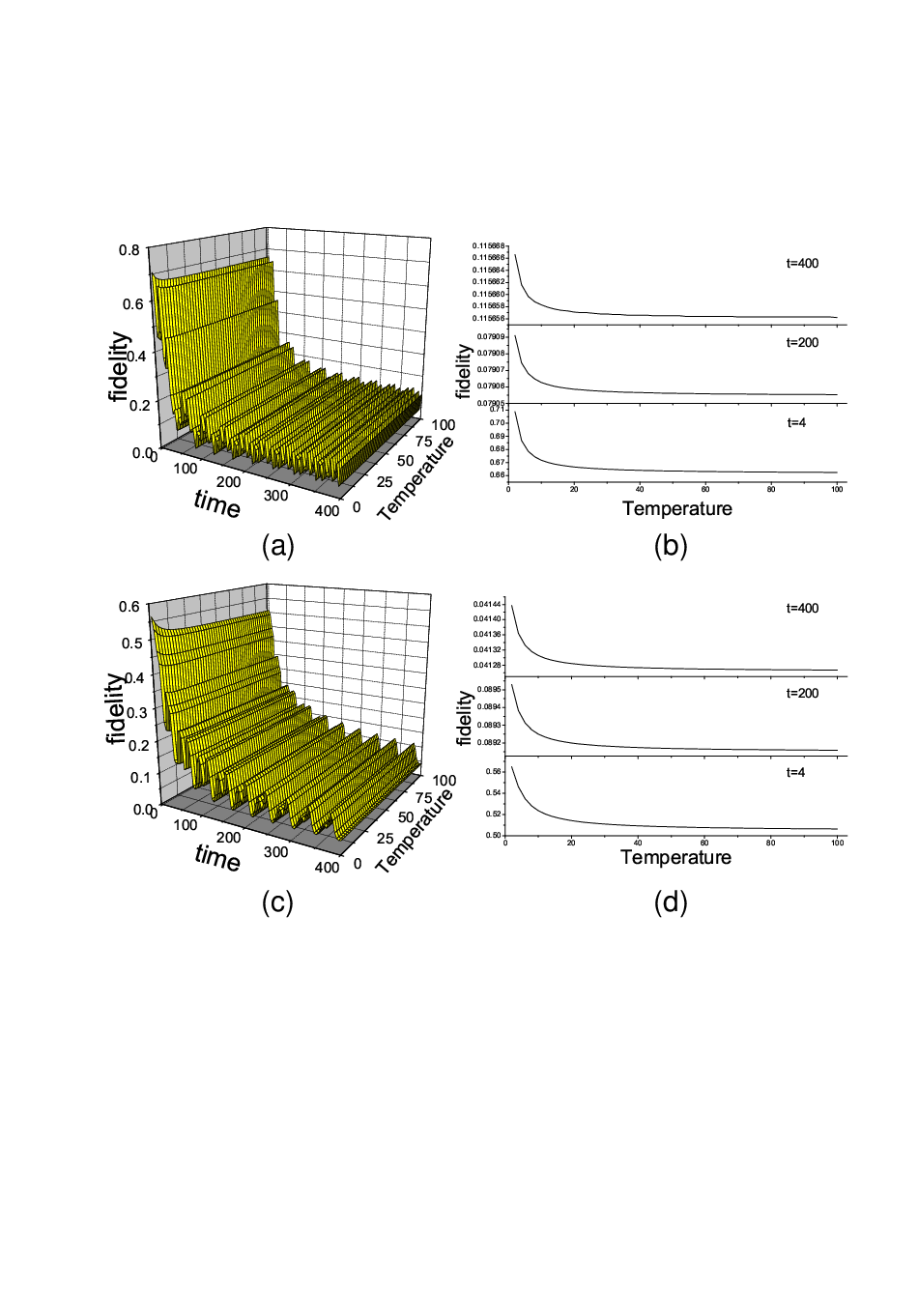

To show the amplitude of the transport state influence, we depicted the fidelity of different states as a function of time and temperature in Fig.2 and Fig.3 respectively, in the case of coupling strength in Eq.(20) and a random Gaussian distribution of the bath energy. Fig. 2 is plotted when the transport state has the form . Fig. 3 is plotted when the transport state is in . Although the fidelity is a decreasing function of time, it can be seen that, from the cross section (b) and (c) in Fig.2 and Fig.3, the amplitude value of transport state determines the temperature effect on fidelity, that is, when the amplitude of state is larger than that of state , the transport efficiency is a descending function of temperature, and when the amplitude of state is smaller than that of state , the transport efficiency is a increasing function of temperature. From the cross section (c) and (d) in Fig.2 and Fig.3, It can be observed that as time increase, the influence of temperature becomes small and small. To show the influence of the site number , in each figure, two 3D diagrams and its cross sections are plotted for different site number of chain. It can be obtained that the fidelity decreases as the number of sites increased. Hence due to exchange of energy between chain and bath, we cannot obtain the original state any longer as time increasing.
VI Summary
In summary, we have investigated the decoherence problem in quantum state transfer (QST). We show when an open spin chain of arbitrary length N interacts with a globe distributed bath, the efficiency of the QST decreases due to the exchange of energy between chain and bath, but the temperature effect on the QST is determined by the form of transport state.
Although our discussion are based on the in the engineered tight binding model with spinless Bloch electrons, it also can be applied to an arbitrary many-particle state in such system. This is because the irreducible tensor method in angular momentum theory could be expected to work well for the QST in an engineered quantum models with more electronsChris1. In the above studies, a qubit is encoded in the superposition of the vacuum and the one-particle state, which is spinless tight binding fermion. Actually, all the conclusions we obtained can be extended to the spin electrons. The electronic wave packet with spin polarization is an analogue of photon “flying qubit”. The spatial fidelity determines the fidelity of freedom of spin.
This work is supported by the NSFC with grant Nos. 90203018, 10474104 and 60433050, and NFRPC with Nos. 2001CB309310 and 2005CB724508. The author Lan Zhou gratefully acknowledges the support of K. C. Wong Education Foundation, Hong Kong.
References
- (1) C. H. Bennett and S. J.Wiesner, Phys. Rev. Lett. 69, 2881 (1992); C. H. Bennett, G. Brassard, C. Cre’peau, R. Jozsa, A. Peres, and W. K. Wootters, Phys. Rev. Lett. 70, 1895 (1993).
- (2) S. Bose, Phys. Rev. Lett. 91, 207901 (2003); D. Burgarth and S. Bose, Phys. Rev. A 71, 052315 (2005); M.-H. Yung and S. Bose, Phys. Rev. A 71, 032310 (2005);
- (3) Michael J. Hartmann, Moritz E. Reuter, Martin B. Plenio, New J. Phys. 8, 94 (2006); M. B. Plenio, J. Hartley and J. Eisert, New J. Phys. 6, 36 (2004); M. B. Plenio, and Semião F. New J. Phys. 7, 73 (2005).
- (4) M. Christandl et al., Phys. Rev. Lett. 92, 187902 (2004); M. Christandl et al., Phys. Rev. A 71, 032312 (2005).
- (5) T. Shi, Ying Li, Z. Song, and C. P. Sun, Phys. Rev. A 71, 032309(2005); Z. Song and C. P. Sun, Low Temp. Phys. 31, 686 (2005); S. Yang, Z. Song, and C. P. Sun, Phys. Rev. A 73, 022317 (2006); S. Yang, Z. Song, and C. P. Sun, Phys. Rev. B 73, 195122 (2006); X.-F. Qian, Y. Li, Y. Li, Z. Song, and C. P. Sun, Phys. Rev. A 72, 062329 (2005); Y. Li, T. Shi, B. Chen, Z. Song, and C.-P. Sun, Phys. Rev. A 71, 022301 (2005).
- (6) Yu-xi Liu, C. P. Sun, and S. X. Yu, Phys. Rev. A 63, 033816 (2001).
- (7) D. Burgarth and S. Bose, Phys. Rev. A 73, 062321 (2006).
- (8) Jian-Ming Cai, Zheng-Wei Zhou, and Guang-Can Guo, quant-ph/0603228.
- (9) W.H. Louisell, Quantum Statistical Properties of Radiation, (Wiley, New York, 1973)