When are correlations quantum? – Verification and quantification of entanglement by simple measurements.

The theoretical and experimental exploration of entanglement and in particular its characterization, verification, manipulation and quantification are key concerns of quantum information science Plenio V 06. The resource character of entanglement is most clearly revealed when dealing with situations in which a locality constraint is imposed, i.e. when distributing the state in such a way that subsequent quantum operations can only act on individual constituents supported by classical communication. This does not only impose constraints on the manipulation and exploitation of entanglement but also on its verification.

In any experiment we will aim to verify the presence of entanglement by taking measurements. These measurements may either serve to reconstruct the entire state or may only collect partial information that is sufficient to reveal the desired entanglement properties Sancho H 00; Horodecki 02; Horodecki 01; Horodecki E 02. Given that a fundamental goal in quantum information science is the creation of entanglement between spatially separate locations one is often forced to assume that these verification measurements are local as well. Generically in such verification experiments we will observe correlations in the measurement record. It is then a natural question whether these correlations originate from quantum correlations in the underlying state or can be explained by a classically correlated separable state. Then, if there are quantum correlations, one can ask how much quantum correlations are guaranteed to be there, given the measurement data.

Consider as an example a two-qubit system and the measurement of correlations between Pauli-operators along the z-axis, i.e. the quantity

where $\rho_{A}$($\rho_{B}$) are the reduced density operators resulting from tracing out party B (A) in the original state $\rho_{AB}$. If ${\cal C}_{zz}(\rho_{AB})=-1$ then the measurement outcomes are perfectly anti-correlated and are thus exhibiting very strong, albeit negative, correlations. Do such correlations imply the existence of quantum correlations in the underlying quantum state? To decide this we must address the following

Fundamental Question: What is the entanglement content of the least entangled quantum state that is compatible with the available measurement data?

Mathematically, this question is formulated as a minimization problem in which the amount of entanglement in the underlying quantum state must be minimized subject to the constraints imposed by the measurement data as well as by the positivity and normalization of the state footnote2. The measurement data will be the expectation values of some observables $A_{i}$ or some non-linear function $F_{i}(\rho)$ of the density matrix. Then the minimal amount of entanglement $E_{\min}$ under the given constraints is given by

where the minimisation domain is the set of states $\rho$ and $E(\rho)$ is the entanglement measure of choice Plenio V 06. Note that this formulation applies equally to the bi-partite as to the multi-partite setting. Note that the importance of the minimization of entanglement in quantum state reconstruction in quantum information theory was also pointed out in the context of Jaynes’ principle Horodecki HH 99.

The mathematical minimization problem formulated by eq. (2) may be addressed by techniques from optimization theory (see e.g. Boyd V 05). If the constraint are all linear and the entanglement quantifier is convex then methods from convex optimization theory may be applied. More complicated constraints that are not linear in the density operator (e.g. purity measures) can complicate matters considerably. Generally it will not be possible to obtain analytic solutions to the optimization problem and techniques to obtain lower bounds or numerical approaches must be used. The analytical and numerical exploration of these issues will be the main purpose of this work.

If the optimal state in eq. (2) is separable, i.e. $E_{\min}=0$, then in reply to our fundamental question we must conclude that the available correlations in the measurement record do not imply quantum correlations in the underlying quantum state. It might be, but need not be entangled. Indeed, in the example given in eq. (1), the least entangled state compatible with the observation ${\cal C}_{zz}(\rho_{AB})=-1$ is given by

which is clearly a separable state. Therefore, the observation of classical correlations for the measurement along one set of directions alone is not sufficient for the verification of entanglement. This well-known observation in quantum information science is particularly relevant in experimental situations where only a very restricted set of measurement settings is available.

One way forward consists in measuring additional observables. For example, one may consider the measurement of

for all spatial directions ${{\vec{n}}}$. Observation of perfect anti-correlations in all of these measurement records then uniquely identifies the singlet state $|\psi\rangle=\frac{1}{\sqrt{2}}(|01\rangle-|10\rangle)$ as the only state compatible with all such measurements. This state carries one ebit of entanglement.

In other experimental situations it may be possible to assert that the state possesses a certain minimal degree of purity Purity, e.g. when decoherence rates, or at least upper bounds for it, are known. Let us for example assume that we know not only that ${\cal C}_{zz}(\rho_{AB})=-1$ but also that $\mathop{\rm Tr}\nolimits[\rho_{AB}^{2}]=1$, i.e. that the underlying quantum state is pure. Then again it is straightforward to conclude that the only states compatible with these two assumptions are of the form

that is, quantum states with one ebit of entanglement.

These simple examples serve to make two points. Firstly, the simple observation of correlations in measurements along a single fixed orientation is not enough to guarantee entanglement in the underlying quantum state. Secondly, additional information, be it correlation measurements along different directions or information about the purity of the states, may be sufficient to ensure that the correlations found in the classical measurement record indeed prove entanglement in the underlying quantum state. Needless to say, in general the situation is quite involved as the measurement data may be more varied than those in the above examples. It should also be noted that the local measurement of the correlation functions mentioned above often implies that we possess more information than just these correlations. Indeed, we will often possess local statistics as well, which in turn can be taken into account when answering our fundamental question concerning the minimal entanglement compatible with the measurement data. Generally, when we are provided with an entangled state, then any additional information will make it less and less likely that the measurement data is compatible with a separable state.

Our fundamental question is of particular relevance in experimental settings in which it is difficult to perform measurements for an arbitrarily large number of measurement settings, as is required for doing full state tomography. This may be the case for example in solid state physics, where it is not always straightforward to perform arbitrary measurements. Another reason may simply be the existence of constraints on the measurement time, dictated for example by the stability time of an experiment (e.g. in interferometric setups in optics) or by the decoherence time (in solid state or other implementations).

The present work shares some relations with Guehne RW 06, Eisert BA 06 and Cavalcanti T 06 where similar questions are developed but where emphasis is placed on observables that are obtained from the theory of entanglement witnesses Witnesses. Other approaches are considered in Mintert B 06; Carteret 05; curty; wolf; toth. While these, as well as the present work, consider the analysis of a specific state, a somewhat different approach is taken in Dynamical. Here the dynamics of the gate used to produce entanglement is considered while measurements are restricted to a single measurement basis. The approach is to make repeated measurements during the gate’s time evolution. This contrasts with our approach which only requires to make measurements on the final state, irrespective of the process that created it.

In this paper we will address our fundamental question for systems consisting only of qubits, as this is by far the most relevant system from an experimental viewpoint. I should be noted however that the approach remains valid unchanged for qudits or even infinite dimensional systems. We begin with an illustration of the general approach in which correlations and purity are quantified by quantum mutual information and global entropy, respectively. While these quantities are not directly experimentally measurable, they allow for the fundamental question to be most easily answered. Then we consider the question for correlations between measurements of Pauli-operators along a single axis, e.g. the z-axis. In the process we prove an inequality between correlations and purity that is valid exactly if a two-qubit state is separable and use it to provide necessary and sufficient conditions for entanglement to be inferred. Subsequently, we consider correlations along two different measurement axes, e.g. x-x correlations and z-z correlations. Finally we consider the situation in which we take into account the local expectation values that are obtained in most experiments to sharpen the verification of entanglement. We finish with some conclusions.

To illustrate the general approach that we are advocating, we begin by considering a situation in which the known system properties are the entropy of the state (determining the state’s purity) and the quantum mutual information (determining the state’s correlation), and in which the entanglement measure of choice is the relative entropy of entanglement Adesso SI 03. The reason for this choice is that there exists a very simple relationship between these quantities, and the solution of the minimization problem eq. (2) is immediate.

The quantum mutual information is given by

and the relative entropy of entanglement is Vedral PRK 97; Vedral P 98; Plenio V 06

For a 2-qubit state, the physically possible values of the pair $(I_{AB},S_{AB})$ are located in a triangle spanned by the points $(0,0)$, $(2,0)$ and $(0,2)$ (see Figure 1). That is, $I_{AB}\geq 0$, $S_{AB}\geq 0$ and $I_{AB}+S_{AB}\leq 2$; equality in the latter inequality is obtained when both reductions $\rho_{A}$ and $\rho_{B}$ are maximally mixed.

The solution to eq. (2) is obtained by applying an inequality lower bounding the relative entropy of entanglement Plenio VP 00 and showing that equality can be achieved for every pair of values of $(I_{AB},S_{AB})$. The inequality is

which directly implies footnote3

The bound is zero in region I ($S_{AB}\geq I_{AB}$) and non-zero in region II ($S_{AB}<I_{AB}$). Equality in region I is obtained by diagonal states; they cover region I completely, and as any diagonal state is separable, they have $E_{R}=0$. Equality in region II is obtained by so-called maximally correlated states, which are of the form

Example 3 of Vedral P 98 shows that these states satisfy

For any given value of $I_{AB}$ and $S_{AB}$ in region II we can find a state of the form eq. (10) realizing these values. By eq. (9) and eq. (11) this state realizes the smallest possible value for the $E_{R}$ given $I_{AB}$ and $S_{AB}$.

The upshot of the results obtained here is that knowledge of the two quantities $S_{AB}$ and $I_{AB}$ allows one to have much better bounds on the entanglement $E_{R}$ than with just knowledge of the correlations $I_{AB}$ alone. Indeed, without knowing the purity $S_{AB}$, one has to assume the worst case, being $S_{AB}=2-I_{AB}$, in which case the lower bound on $E_{R}$ is given by

If, on the other hand, the state is known to be pure, say, ($S_{AB}=0$) then the much sharper bound

can be obtained.

In the rest of the paper we will apply the approach illustrated here for studying the main question eq. (2) in the context of experimentally accessible quantities. In the next Section the measure of correlation will be based on measurements along the z-axis. It will turn out that without knowledge of the purity one cannot find any lower bound on entanglement other than the trivial bound $E\geq 0$. Thus, while in the present Section one can get some information about the entanglement from the quantum mutual information without knowledge of the purity, in the next Section knowledge of the purity is absolutely essential.

In a number of experimental settings it is not straightforward to carry out measurements along arbitrary directions. To obtain a measure of correlation in those settings, one can for example consider the quantity

which only requires measurements along the particles’ $z$-axes. However, in the previous Section we already alluded to the fact that knowledge of this correlation measure alone is not sufficient to prove the presence of quantum entanglement. We will establish that fact in the present Section. Moreover, we will show that if in addition the purity of the state is known, as quantified by

and provided this purity is large enough, then and only then can one infer entanglement from the z-correlation measure.

Now the question is: how pure does the underlying quantum state have to be so that $|{\cal C}_{zz}|>0$ indeed implies quantum entanglement? Or, more precisely:

When are all states consistent with given values of ${\cal C}_{zz}$ and ${\cal P}$ non-separable, and what is the least entanglement compatible with these values?

It turns out that the rigorous analytical answer is surprisingly involved, largely due to the non-linearity of the constraints involved in the minimization problem, especially if one is also interested in the actual amount of entanglement that can be guaranteed from such measurements.

As measure of entanglement we have used the logarithmic negativity $E_{N}$, because this is the measure that is most easily calculated footnote. The log-negativity is defined as

where $\Gamma$ denotes partial transposition w.r.t. subsystem B.

In Figure 2, we present our numerical results on the smallest amount of entanglement compatible with given values of purity (see eq. (13)) and of correlations in the measurement record (see eq. (12)). This numerical evaluation suggests the following:

• •

  Region I does not allow for any physical states.

• •

  There is a well-defined central region $S$ that does not allow to infer the presence of entanglement as the values for purity and correlations can be reproduced by a separable state.

• •

  Only in regions IIa and IIb is entanglement guaranteed. The minimal value of $E_{N}$ in those regions is given by

  $$E_{N}\geq\log_{2}(1+\sqrt{2(Q-1)+{\cal C}_{zz}}),$$

  (14)

  in Region IIa, and

  $$E_{N}\geq\log_{2}({\cal C}_{zz}+\sqrt{2Q-1})$$

  (15)

  in Region IIb. Here, $Q=\mathop{\rm Tr}\nolimits[\rho^{2}]=(3{\cal P}+1)/4$.

One may either calculate both bounds and take the minimum, or infer which region one is in via the limits

which hold for Region IIa.

We stress that we do not have a complete proof of these statements. They were derived – in a rather laborious way – starting from an Ansatz concerning the form of the states achieving the bounds. This Ansatz was in turn obtained from a combination of Monte-Carlo calculations and inspired guess-work. While a proof does not seem forthcoming, the numerical evidence for correctness of the Ansatz, and of the bounds derived from them, is very convincing. The interested reader is advised to contact the authors for further details.

Analytical proof of boundaries – What we do have been able to prove is the analytical form of the boundaries of the $S$ region, the region where be separable states. They are given by

Here, the first inequality defines the boundary with Region I while the second one defines the boundary with Region IIa.

To proceed, we treat boundary I and II separately. For boundary I we can simplify the form of $\rho$ that needs to be considered quite significantly. To this end note that correlations ${\cal C}_{zz}(\rho)$ are unaffected by the transformation

ie, ${\cal C}_{zz}(\rho)={\cal C}_{zz}({\bar{\rho}})$ but at the same time the transformation from $\rho$ to ${\bar{\rho}}$ reduces purity as they correspond to pinchings Bhatia. A state ${\bar{\rho}}$ that is invariant under the above maps is diagonal. As these maps are local we find that if $E(\rho)=0$, then $E({\bar{\rho}})=0$. To determine the boundary I let us now fix a value for ${\cal C}_{zz}$ and determine the smallest purity compatible with it. If we have a $\rho$ with a given purity then by the above transformations we can find a ${\bar{\rho}}$ with the same ${\cal C}_{zz}$ and no larger purity that is diagonal. Therefore it is sufficient to restrict attention from the outset to diagonal $\rho$, i.e. $\rho=\mathop{\rm Diag}\nolimits(a,b,c,1-a-b-c)$. Then we find ${\cal C}_{zz}=1-2b-2c$ and the purity is given by

Without restriction of generality we assume ${\cal C}_{zz}\geq 0$ (the case ${\cal C}_{zz}\leq 0$ can be treated analogously) and one finds that the purity is minimized for $b=c$. This leaves us with the minimization of the expression

for

Then the minimal purity compatible with the given ${\cal C}$ is then found to be

yielding the boundary confirming eq. (17).

Determining the boundary II is more involved and is based on the observation that for all separable states $\rho$ we have Hall AB 06

We first note that $\mathop{\rm Tr}\nolimits[\rho^{2}]+\frac{1}{2}{\cal C}_{zz}(\rho)$ is convex in $\rho$. Indeed, a short calculation reveals that this expression is equal to

As every term is convex in $\rho$, the total expression is. Therefore, the inequality only has to be checked for the extremal points of the set of separable states, i.e. for pure product states. This, however, is very easy: for product states, ${\cal C}_{zz}=0$, and for pure states $\mathop{\rm Tr}\nolimits[\rho^{2}]=1$, whence the inequality is satisfied with equality.

Now we note that the separable states $\rho=a|00\rangle\langle 00|+(1-a)|11\rangle\langle 11|$ saturate the bound (22). Rewriting this bound in terms of ${\cal P}(\rho)$ we find ${\cal P}\leq 1-2{\cal C}_{zz}/3$. This then completes the proof for boundary II.

A lower bound for $E_{N}$ – As mentioned above, we have not been able to prove our lower bounds (14) and (15) so far. Nevertheless, inequality (22) suggests that

might be a lower bound on the entanglement in all regions. Here we define the function $\log_{2}^{+}(x):=\max(0,\log_{2}(x))$; that is, $\log_{2}^{+}(x)=0$ for $x\leq 1$. We will prove eq. (23) in subsection VII, where a general recipe for the derivation of such bounds is presented.

Let us now move away from the use of non-linear properties of the density operator such as purities or entropies and consider only linear functionals, i.e. expectation values of quantum mechanical operators that are directly accessible to experimental detection. Consider the case when we are given the quantities

(note that these are different quantities than the one used in the previous Section). In this case it is quite straightforward to determine the minimal entanglement compatible with any choice of $C_{xx}$ and $C_{zz}$. To see this we first realize that $C_{xx}$ and $C_{zz}$ are invariant under the transformation

Thus for given $C_{xx}$ and $C_{zz}$ we may restrict attention to states of the form

Let us now consider the case $C_{xx}\geq 0$ and $C_{zz}\geq 0$. Any other choice can be reduced to this one by application of $\mathrm{\openone}\otimes\sigma_{x}$ or $\mathrm{\openone}\otimes\sigma_{z}$ onto the state.

The requirements for positivity of $\rho$ are $b\leq(1-C_{zz})/4$ and $C_{xx}/2-b\leq(1+C_{zz})/4$. From the first requirement follows that $|b|\leq(1+C_{zz})/4$. Thus any amount of negativity of the partial transpose of $\rho$ must arise from $\rho_{14}=C_{xx}/2-b$. As we are looking for the smallest amount of entanglement compatible with the choice $C_{xx},C_{zz}\geq 0$, we must minimize $C_{xx}/2-b$, i.e. maximize $b$. This is achieved by the choice $b=(1-C_{zz})/4$; one checks that this choice satisfies the second requirement $C_{xx}/2-b\leq(1+C_{zz})/4$. Then we find $E_{\min}(C_{xx},C_{zz})=\log_{2}^{+}(C_{xx}+C_{zz})$. For general $C_{xx},C_{zz}$ we find

This result may easily be generalized to the case of three correlations

for which we find

If the sub-systems for which we would like to verify entanglement are distant, then any measurement strategy has to be composed of local measurements. In this way we can, of course, still obtain averages such as $\langle\sigma_{x}\otimes\sigma_{x}\rangle$ by measuring local observables (such as $\sigma_{x}$) and use these averages to determine correlations (such as $C_{xx}$). While the assessment of entanglement wil primarily depend on the values of these correlations, it is important to note that these local measurements will in addition yield local averages (such as $\langle\sigma_{x}\rangle$), which by themselves are not useful to assess entanglement, but when taken together with the correlation values represent additional knowledge that we can and should take account of. Note that the question of the verification of the presence of entanglement in the particular setting considered in this section has been addressed in curty. The full analytical treatment of the quantification of the least amount of entanglement compatible with the measurement data in this setting is quite complicated due to the large number of possibilities that are available. In the following we will simply present an example to illuminate the impact that additional local information may have on the question of assessing least entanglement compatible with the measurement data.

Let us reconsider the case in which we employed $C_{zz}=\mathop{\rm Tr}\nolimits[(\sigma_{z}^{(1)}\otimes\sigma_{z}^{(2)})\rho]$ and $C_{xx}=\mathop{\rm Tr}\nolimits[(\sigma_{x}^{(1)}\otimes\sigma_{x}^{(2)})\rho]$. In this setting we found that $E_{\min}(C_{xx},C_{zz})=\log_{2}^{+}(C_{xx}+C_{zz})$ (eq. (26)). Let us now investigate what can be gained by taking into account knowledge of $z_{1}:=\mathop{\rm Tr}\nolimits[\sigma_{z}^{(1)}\rho]$ and $z_{2}:=\mathop{\rm Tr}\nolimits[\sigma_{z}^{(2)}\rho]$; that is, we determine the minimal amount of entanglement compatible with the information given in $C_{xx},C_{zz}$ and $z_{1},z_{2}$.

We can no longer restrict ourselves to states of the form (25), because $z_{1}$ and $z_{2}$ are not invariant under transformations (24). The optimal states can now be assumed to possess a $\sigma_{z}\otimes\sigma_{z}$ symmetry. The diagonal elements of the optimal $\rho$ are fully determined by $C_{zz},z_{1},z_{2}$ and $\mathop{\rm Tr}\nolimits[\rho]=1$. Employing the $\sigma_{z}\otimes\sigma_{z}$ symmetry of the system the problem can be reduced to a single-parameter minimisation. The optimal states turn out to be of the form

with

and

Given $z_{1}$ and $z_{2}$, there are now restrictions on the values of $C_{xx}$ and $C_{zz}$:

The negative eigenvalue of the partial transpose of $\rho$ is given by

The log-negativity $E_{N}$ is then

To minimise $E_{N}$, we have to maximise $\lambda_{\min}$ over all allowed values of $e$, which is the range

As an example, in Figure 3, we present the difference between the minimal compatible entanglement for given $(C_{zz}=1-|z_{1}-z_{2}|=0.9,C_{xx},z_{1}=0.3,z_{2}=0.2)$ and the one when only $(C_{zz}=0.9,C_{xx})$ are given. For the given value of $C_{zz}$, either $b=0$ or $c=0$, so that the only allowed value for $e$ is $e=0$, giving

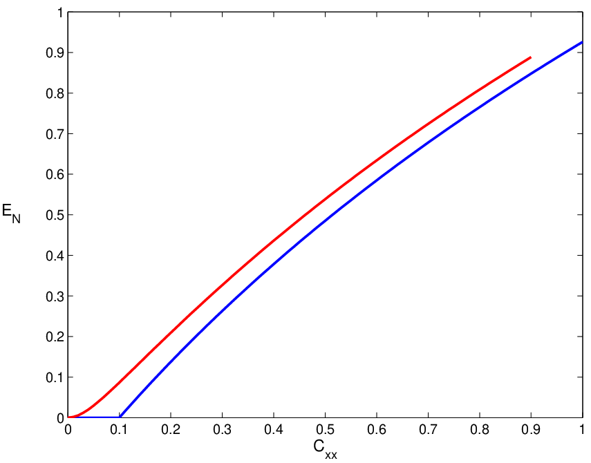
While, of course, the parameter range for which physical density operators compatible with those data exist is more limited in the former case, it is indeed apparent that the knowledge of $C_{xx}$ and $C_{zz}$ in combination with $z_{1},z_{2}$ allows us to infer a larger amount of entanglement.

This example highlights the importance of including all available information in the entanglement verification as it may substantially alter our conclusions. The exact details of the procedure will, of course, depend on the concrete situation.

Our considerations are not restricted to bi-partite entanglement. Again, quite general observables may be considered but in line with the bi-partite case we illustrate this setting for a simple set of observables. Let us consider the expectation values $C_{xxx}=\langle\sigma_{x}\otimes\sigma_{x}\otimes\sigma_{x}\rangle$, $C_{1zz}=\langle\mathrm{\openone}\otimes\sigma_{z}\otimes\sigma_{z}\rangle$ and $C_{zz1}=\langle\sigma_{z}\otimes\sigma_{z}\otimes\mathrm{\openone}\rangle$. Given the symmetries that leave these expectation values invariant, we may restrict attention to density operators of the form ¹¹ 1 Note that these states are diagonal in the GHZ-basis made up of the state $(|000\rangle\pm|111\rangle)/\sqrt{2}$, $(|001\rangle\pm|110\rangle)/\sqrt{2}$, $(|010\rangle\pm|101\rangle)/\sqrt{2}$ and $(|011\rangle\pm|100\rangle)/\sqrt{2}$.

In the tripartite setting it is considerably more difficult than in the bi-partite setting to define entanglement measures Plenio V 06. We consider two entanglement measures, the relative entropy of entanglement and the robustness of enanglement.

We begin with the relative entropy of entanglement with respect to Tri-PPT states, i.e. states that are PPT with respect to any of the three possible bi-partite cuts

It is helpful to note that it is always sufficient to restrict the minimization over $\rho$ to those states that possess the same local symmetries as $\sigma$ Vedral PRK 97; Vedral P 98. Thus only states $\rho$ of the form eq. (29) need to be considered. These states all commute with $\sigma$. Thus we are looking for a two-fold minimization

We note that states $\sigma$ of the form eq. (29) are Tri-PPT if and only if $\Delta=\max\{|e|,|f|,|g|,|h|\}-\min\{a,b,c,d\}\leq 0$. Due to unitary invariance of the relative entropy we can apply local unitaries to both $\rho$ and $\sigma$; one can therefore restrict to non-negative real $e$, $f$, $g$ and $h$. Defining $m:=\min\{a,b,c,d\}$ we obtain the restrictions $e,f,g,h\leq m$.

The expectation values for such states are given by

Note that these expectation values lie in the range $[-1,1]$.

The minimisation over $\rho$ reduces to a three-parameter minimisation. Let the matrix elements of $\sigma$ and $\rho$ (in the form (29)) be denoted $a_{\sigma}$, $a_{\rho}$, etc. The three parameters are $a_{\rho}$, $b_{\rho}$ and $c_{\rho}$. The other matrix elements of the optimal $\rho$ are given by

where $m_{\rho}:=\min\{a_{\rho},b_{\rho},c_{\rho},d_{\rho}\}$. The expression for the relative entropy in this optimal state is

with three additional terms of obvious form. Here, $H$ is the classical (Kullback-Leibler) relative entropy between two (unnormalised) two-dimensional probability vectors.

Because of joint convexity of the relative entropy, and convexity of the feasible set for $\rho$, the remaining minimisation (over $\rho$ and $\sigma$) is a convex one, which means that there can only be one local minimum. It can therefore be efficiently calculated numerically using, e.g. conjugate gradient methods. We have performed numerical calculations based on this method, and plotted the results in Figure 4 for the example of $C_{xxx}=1$.

Another possible entanglement quantifier is the random robustness $R(\sigma)$ robustness. The random robustness is defined as the minimal amount of the maximally mixed state $\mathrm{\openone}/d$ that needs to be mixed with $\sigma$ to make the resulting state Tri-PPT. Formally,

We find that

Therefore, the minimal robustness under the constraints $C_{xxx}=\langle\sigma_{x}\otimes\sigma_{x}\otimes\sigma_{x}\rangle$, $C_{1zz}=\langle\mathrm{\openone}\otimes\sigma_{z}\otimes\sigma_{z}\rangle$ and $C_{zz1}=\langle\sigma_{z}\otimes\sigma_{z}\otimes\mathrm{\openone}\rangle$ is given by

where

In this Section, we readdress some of the issues of Section III. It is worth noting that the last result obtained there, eq. (27), could have been obtained from a general strategy to obtain lower bounds for the minimization problem eq. (2).

This can be achieved by using the fact that $||\rho^{\Gamma}||_{1}=\max_{||M||_{\infty}=1}\mathop{\rm Tr}\nolimits[M\rho^{\Gamma}]=\max_{||M||_{\infty}=1}\mathop{\rm Tr}\nolimits[M^{\Gamma}\rho]$, where the maximization is over Hermitian $M$ Bhatia. Thus we consider the problem

where the outer minimization is over positive semidefinite matrices $\rho$ (the trace condition for states is included by putting $A_{0}=\mathrm{\openone}$, $a_{0}=1$), and the inner maximisation is over all Hermitian matrices $M$. When $F_{i}$ is a convex function its level sets $\{\rho:F_{i}(\rho)\leq f_{i}\}$ are convex sets, and we can use the minimax equality (see e.g. Boyd V 05) to interchange inner and outer optimisations, obtaining

Let us now consider the case that there are no non-linear constraints $F_{i}$, then the inner minimization is a semidefinite program (SDP). We now apply Lagrange duality to this minimization, i.e. we consider the unconstrained minimization of the Lagrangian $\min_{\rho}\mathop{\rm Tr}\nolimits[(M^{\Gamma}-\sum\nu_{i}A_{i})\rho]+\sum_{i}\nu_{i}a_{i}$ over all positive semidefinite $\rho\geq 0$, where the $\nu_{i}$ are the Lagrange multipliers. If $M^{\Gamma}-\sum\nu_{i}A_{i}$ has negative eigenvalues, the minimum of the Lagrangian will be $-\infty$ (by letting $\rho$ become arbitrarily large), and will not contribute to the outer maximization over $M$. Thus we can safely require $M^{\Gamma}-\sum\nu_{i}A_{i}\geq 0$, in which case the minimum is obtained for $\rho=0$ and equals $\sum_{i}\nu_{i}a_{i}$. Inserting this we find

Because the inner minimization is an SDP, if the problem is strictly feasible, i.e. if all inequality constraints can be satisfied with strict inequalities, then we have strong duality Boyd V 05 and the above step does not weaken the lower bounds.

Any choice of $M$ and $\nu_{i}$ such that $M^{\Gamma}\geq\sum_{i}\nu_{i}A_{i}$ and $||M||_{\infty}=1$ now yields a lower bound on $E_{\min}$. Indeed, this could have been read off immediately from eq. (38). However, as the optimization problem eq. (39) shows this may be overly restrictive. See Guehne RW 06; Eisert BA 06 for lower bounds on other entanglement measures.

Applications – In the case of given $(C_{xx},C_{zz})$ with $C_{xx}+C_{zz}\geq 1$ as discussed in Section IV, we have $A_{0}=\mathrm{\openone}$, $A_{1}=\sigma_{x}\otimes\sigma_{x}$ and $A_{2}=\sigma_{z}\otimes\sigma_{z}$, and $a_{0}=1$, $a_{1}=C_{xx}$ and $a_{2}=C_{zz}$. In this case we find as optimal $M$:

(which indeed has operator norm 1) and as optimal $\nu_{i}$: $\nu_{0}=0,\nu_{1}=\nu_{2}=1$. One checks that $M^{\Gamma}\geq A_{1}+A_{2}$. From this we recover again eq. (26).

For the case of given $(C_{xx},C_{yy},C_{zz})$ we choose $\nu_{0}=\nu_{1}=\nu_{3}=1/2,\nu_{2}=-1/2$, so that $\sum_{i}\nu_{i}A_{i}=(\mathrm{\openone}+\sigma_{x}\otimes\sigma_{x}-\sigma_{y}\otimes\sigma_{y}+\sigma_{z}\otimes\sigma_{z})/2$. Taking $M=(\mathrm{\openone}+\sigma_{x}\otimes\sigma_{x}+\sigma_{y}\otimes\sigma_{y}+\sigma_{z}\otimes\sigma_{z})/2$ (which has operator norm 1) yields $M^{\Gamma}=\sum_{i}\nu_{i}A_{i}$, and we recover the exact value found in eq. (27).

Proof of eq. (23) – A similar approach may suggest itself for the case concerning purity and correlations discussed in section III and will be used to prove the lower bound eq. (23). The constraints are however non-linear. To proceed, we will use a kind of linearization procedure. We begin by rewriting the quantities ${\cal C}_{zz}(\rho)$ and $\mathop{\rm Tr}\nolimits[\rho^{2}]$ in terms of expressions linear in the tensor product $\tau:=\rho\otimes\rho$. Taking into account $\mathop{\rm Tr}\nolimits[\rho]=1$ we find

where $Z$ is the operator

and $F$ is the flip operator that interchanges parties $1,2$ of the first copy with parties $3,4$ of the second. The $Z$ presented here is the simplest one that represents ${\cal C}_{zz}$. However, it is beneficial to use the symmetrised form $Z^{\prime}=(Z+FZF)/2$.

Let us now address the minimization of $\frac{1}{2}\log_{2}||\rho^{\Gamma}\otimes\rho^{\Gamma}||_{1}$ given constraints on ${\cal C}_{zz}(\rho)$ and $\mathop{\rm Tr}\nolimits[\rho^{2}]$. This problem is linear in $\sigma=\rho\otimes\rho$ and is therefore an SDP. Consequentially, we can apply the above approach. Indeed, let us choose $M=\mathop{\rm Diag}\nolimits(1111\;1101\;1011\;1111)$. Then, clearly, $M^{\Gamma}-Z^{\prime}/2-F\geq 0$ and we obtain eq. (23) as a lower bound on the entanglement. This bound is certainly not tight, however. Indeed, we could not have expected much more, as the extension of the problem to two copies allowed for much greater freedom in the matrix $M$ and, therefore, led us to underestimate the true value of $E_{\min}$.

In this work we have pointed out that in an experimental verification of entanglement we need to search for the least entangled state compatible with the measured data. If the state so identified is entangled then the experimental data prove the presence of entanglement. This approach is not restricted to the verification of entanglement. In fact, it applies to any physical property that we cannot or chose not to measure directly.

Consider the property $\Pi$ of a quantum system which is quantified by $\Pi(\rho)$. If we are obtaining experimental data, for example quantum mechanical averages of some observables $A_{i}$, then we need to answer the

Fundamental Question: What is the least value of $\Pi$ for which there is a state that is compatible with the available measurement data?

This smallest value of $\Pi$ is the value to which we have verified the presence of $\Pi$. Mathematically this may again be formulated as a minimization problem in which the property $\Pi$ in the underlying quantum state must be minimized subject to the positivity, Hermiticity and normalization and measurement data obtained as expectation values of observables $A_{i}$ or some non-linear function $F_{i}(\rho)$ of the density matrix. Then the minimal amount of entanglement $E_{\min}$ under the given constraints is given by

where the minimisation domain is the set of states $\rho$.

In this more general framework the minimization of entanglement is merely a special case of a general approach to the verification of physical properties in experiments.

In this work we have addressed the question of when correlations or other measurement data that have been observed in the classical measurement record of a quantum system imply the existence of quantum correlations in the underlying state. The fundamental question in this area may be formulated as: What is the entanglement content of the least entangled quantum state that is compatible with the available measurement data? We have formulated this question mathematically as an optimization problem, discussed it for various examples and provided some techniques for obtaining non-trivial lower bounds on the minimal entanglement compatible with the measurement data. The approach is equally valid in the bi-partite and the multi-partite setting and for sub-systems of arbitrary dimensionality. We hope that these investigations will be helpful in experimental efforts that aim at the creation and subsequent unequivocal verification and quantification of the generated entanglement. This should, in particular, apply to experimental set-ups where for various reasons only a limited number of measurement settings is available.

Acknowledgements – We thank Alvaro Feito for careful reading of the manuscript and helpful suggestions. We are grateful to Pawel Horodecki for bringing ref. Horodecki HH 99 to our attention. We also thank an anonymous referee for pointing out a simpler proof of eq. (22) than the one contained in an earlier version.

References

- (1) M.B. Plenio and S. Virmani, Quant. Inf. Comp. 7, 1 (2007), E-print arXiv quant-ph/0504163.
- (2) J.M.G. Sancho and S. F. Huelga, Phys. Rev. A 61, 042303 (2000).
- (3) P. Horodecki, Phys. Rev. Lett. 90, 167901 (2002).
- (4) P. Horodecki, quant-ph/0110036.
- (5) P. Horodecki and A. Ekert, Phys. Rev. Lett. 89, 127902 (2002).
- (6) Note that, while formally not dissimilar, this fundamental question is from a physical point of view quite different from that concerning the maximization under some constraints (see for example the concept of maximally entangled mixed states Ishizaka H 00; Verstraete AD 01).
- (7) S. Ishizaka and T. Hiroshima, Phys. Rev. A 62, 022310 (2000).
- (8) F. Verstraete, K. Audenaert and B. De Moor, Phys. Rev. A 64, 012316 (2001).
- (9) R. Horodecki, M. Horodecki, and P. Horodecki, Phys. Rev. A 59, 1799 (1999).
- (10) S. Boyd and L. Vandenberghe, Convex Optimization, Cambridge University Press 2005.
- (11) O. Gühne, M. Reimpell, and R.F. Werner, E-print arxiv quant-ph/0607163.
- (12) J. Eisert, F.G.S.L. Brandão and K. Audenaert, E-print arxiv quant-ph/0607167.
- (13) M. Horodecki, P. Horodecki and R. Horodecki, Phys. Lett. A 223, 1 (1996); B.M. Terhal, Phys. Lett. A 271, 319 (2000).
- (14) F. Mintert and A. Buchleitner, E-print arxiv quant-ph/0605250.
- (15) H. Carteret, Phys. Rev. Lett. 94, 040502 (2005).
- (16) M. Curty, M. Lewenstein and N. Lütkenhaus, Phys. Rev. Lett. 92, 217903 (2004).
- (17) M.M. Wolf, G. Giedke and J.I. Cirac, Phys. Rev. Lett. 96, 080502 (2006).
- (18) G. Toth and O. Gühne, Phys. Rev. Lett. 94, 060501 (2005).
- (19) D. Cavalcanti and M.O. Terra Cunha, E-print arxiv quant-ph/0605155.
- (20) B. Schelpe, A. Kent, W. Munro and T. Spiller, Phys. Rev. A 67, 052316 (2003).
- (21) A similar setting has been analyzed for the logarithmic negativity in the Gaussian continuous variable setting in G. Adesso, A. Serafini and F. Illuminati, Phys. Rev. A 70, 022318 (2004); G. Adesso, A. Serafini and F. Illuminati, Phys. Rev. Lett. 92, 087901 (2004); G. Adesso, A. Serafini, and F. Illuminati, Phys. Rev. Lett. 93, 220504 (2004) and the qubit setting in D. McHugh, M. Ziman and V. Buzek, E-print arxiv quant-ph/0607012.
- (22) W.K. Wootters, Phys. Rev. Lett. 80, 2245 (1998); P. M. Hayden, M. Horodecki, and B. M. Terhal, J. Phys. A 34, 6891 (2001).
- (23) V. Vedral, M.B. Plenio, M.A. Rippin and P.L. Knight, Phys. Rev. Lett. 78, 2275 (1997); V. Vedral, M.B. Plenio K.A. Jacobs and P.L. Knight, Phys. Rev. A 56, 4452 (1997).
- (24) V. Vedral and M.B. Plenio, Phys. Rev. A 57, 1619 (1998).
- (25) M.B. Plenio, S. Virmani and P. Papadopoulos, J. Phys. A 33, L193 (2000).
- (26) It should be noted that the same lower bound also holds true for the asymptotic relative entropy of entanglement Audenaert EJPVD 01 as the lower bounds derived here are in fact additive.
- (27) K. Audenaert, J. Eisert, E. Jane, M.B. Plenio, S. Virmani and B. De Moor, Phys. Rev. Lett. 87, 217902 (2001).
- (28) For qubits the logarithmic negativity Plenio 05; Plenio V 06 is the entanglement cost under exact preparation using PPT-preserving operations Audenaert PE 03 which in turn is larger than the entanglement cost under PPT-preserving operations. This is lower bounded by the quantum relative entropy of entanglement with respect to PPT-states. For qubits, however, this is the same as the relative entropy with respect to separable states, so that we have the same lower bound on the logarithmic negativity in the plot.
- (29) M.B. Plenio, Phys. Rev. Lett. 95, 090503 (2005); J. Eisert and M.B. Plenio, J. Mod. Opt. 46, 145 (1999); J. Eisert, PhD Thesis Potsdam 2001; G. Vidal and R. F. Werner, Phys. Rev. A 65, 32314 (2002); J. Lee, M.S. Kim, Y.J. Park and S. Lee, J. Mod. Opt. 47, 2151 (2000).
- (30) K. Audenaert, M.B. Plenio and J. Eisert, Phys. Rev. Lett. 90, 027901 (2003).
- (31) R. Bhatia, Matrix Analysis, Springer New York 1997.
- (32) Following the publication of the preprint version quant-ph/0608067 of the present work a generalization of eq. (22) was presented in M.J.W. Hall, E. Andersson and T. Brougham, E-print arxiv quant-ph/0609076.
- (33) E. Bagan, M.A. Ballester, R. Muñoz-Tapia, and O. Romero-Isart, Phys. Rev. Lett. 95, 110504 (2005); M.G.A. Paris, F. Illuminati, A. Serafini and S. De Siena, Phys. Rev. A 68, 012314 (2003).
- (34) G. Vidal and R. Tarrach, Phys. Rev. A 59, 141–155 (1999).