On the Relationship between Resolution Enhancement and Multiphoton Absorption Rate in Quantum Lithography
Abstract
The proposal of quantum lithography [Boto et al., Phys. Rev. Lett. 85, 2733 (2000)] is studied via a rigorous formalism. It is shown that, contrary to Boto et al.’s heuristic claim, the multiphoton absorption rate of a “NOON” quantum state is actually lower than that of a classical state with otherwise identical parameters. The proof-of-concept experiment of quantum lithography [D’Angelo et al., Phys. Rev. Lett. 87, 013602 (2001)] is also analyzed in terms of the proposed formalism, and the experiment is shown to have a reduced multiphoton absorption rate in order to emulate quantum lithography accurately. Finally, quantum lithography by the use of a jointly Gaussian quantum state of light is investigated to illustrate the trade-off between resolution enhancement and multiphoton absorption rate.
pacs
42.50.Dv, 42.50.StI Introduction
Optical lithography, the process in which spatial patterns are transferred via optical waves to the surface of a substrate, has been hugely successful in the fabrication of micro and nanoscale structures, such as semiconductor circuits and microelectromechanical systems. Conventional lithography cannot produce features much smaller than the optical wavelength, due to the well known Rayleigh resolution limit bornwolf. As a result, beating the resolution limit for lithography has become an important goal in the field of optics, with far-reaching impact on other research areas including semiconductor electronics and nanotechnology.
Among the many candidates proposed to supersede conventional lithography, the use of extreme ultraviolet light for lithography gwyn has met numerous technical difficulties such as optics imperfections and photoresist limitations. Other proposals involve multiphoton exposure yablonovitch; boto; agarwal; bentley; hemmer, so that one can still use the more robust optics for long-wavelength light, while obtaining some of the resolution improvements associated with higher harmonics. The feature size reduction, however, is not nominal without taking care of the residual long-wavelength features in a multiphoton absorption pattern. Yablonovitch and Vrijen proposed the use of several frequencies and narrowband two-photon absorption to suppress such long-wavelength features yablonovitch, while a much more radical proposal by Boto et al. suggests the use of -photon quantum interference of spatially entangled photons boto. The so-called quantum lithography has several appeals, such as arbitrary quantum interference patterns, generalization to arbitrary number of photons, and the promise of multiphoton absorption rate improvement via the use of entangled photons. Hence, despite practical issues such as difficulties in generating a high dosage of the requisite entangled photons and finding a suitable multiphoton resist, interest in quantum lithography has been significant boyd.
Crucial to the future success of quantum lithography is the supposed enhancement in the multiphoton absorption rate when entangled photons are used. The absorption rate improvement for frequency anticorrelated photons has been proved by Javanainen and Gould javanainen and Perina et al. perina. Boto et al. further claimed that the absorption rate should also improve for the spatially entangled photons used in quantum lithography. This promise is absolutely vital to the practicality of quantum lithography, because, as Boto et al. mentioned, classical multiphoton lithography is already infeasible for large , and quantum lithography would have been even worse if the absorption rate was not enhanced, due to the much less efficient generation of nonclassical light. Boto et al. supported their claim by arguing heuristically that the entangled photons are constrained to arrive at the same place and at the same time. This argument with respect to the spatial domain has, however, not been substantiated with a more rigorous proof, and has been subject to criticism steuernagel. Unfortunately, the time domain treatment javanainen; perina cannot be directly carried over to the spatial domain, because the former assumes a nearly resonant multiphoton absorption process and does not require any temporal resolution, but for quantum lithography the material response needs to be spatially local to produce a high spatial resolution.
On the other hand, Boto et al.’s formalism contains several crucial approximations that remain to be justified. First, the photons are implicitly assumed to arrive from a monochromatic source with a well defined free-space wavelength , but the usual quantization method of optical fields considers photons as quanta of electromagnetic mode excitations, in which frequency appears only as a dependent variable of the wave vector. It remains a question how monochromatic optical fields as a boundary condition should be treated in quantum optics. Second, they treat the two optical beams with opposite transverse momenta as two discrete modes of optical fields, but in free space, transverse momentum is a continuous variable, so the discrete modes are evidently an approximation. Third, when discussing the multiphoton absorption rate, Boto et al. regards photons as objects in space and time that probabilistically arrive at the photoresist, although it is well known that this interpretation of photons is fundamentally flawed mandel.
In this paper, starting from basic principles, I shall first explicitly quantize the electromagnetic fields in Sec. II, using assumptions consistent with Boto et al.’s proposal. The formalism rigorously treats approximately monochromatic optical fields as a boundary condition in the continuous Fock space, and hence provides a theoretical underpinning to the proposal of quantum lithography. The formalism also shows that, regardless of the nonclassical spatial properties of the photons, there exists an upper bound of multiphoton absorption rate, which rules out any significant enhancement of multiphoton absorption rate due to spatial effects only. Next, using the developed formalism, I shall analyze in Sec. III the multiphoton absorption rate of the so-called NOON state, and compare it with that of a classical state with otherwise identical parameters. The analysis shows that, despite both states having the same envelope for their interference fringes, and despite the NOON state being able to reduce the interference period of the fringes by a factor of , the peak multiphoton absorption rate of a NOON state is lower than that of a classical state by a factor of . In Sec. IV, I shall discuss the formalism in the paraxial regime, where it is acceptable to regard photons as spatial objects described by a configuration-space probability density. I shall then investigate the proof-of-concept quantum lithography experiment by D’Angelo et al. dangelo and show that the experiment requires a condition that necessarily reduces the two-photon absorption rate, in order to emulate quantum lithography accurately. Finally, I shall study the multiphoton absorption of a jointly Gaussian multiphoton state, in order to illustrate the trade-off between resolution enhancement and multiphoton absorption rate.
II Quantization of Two-Dimensional, S-Polarized, Approximately Monochromatic Electromagnetic Fields
II.1 Two Dimensional Approximation
I shall start with the most general commutation relations for creation and annihilation operators of continuous electromagnetic field modes in free space mandel:
| (1) |
where , , and are the independent continuous variables for each mode of the electromagnetic fields, and denotes one of the two polarizations perpendicular to the wave vector. The dependent variable in this case is frequency , determined by the dispersion relation
| (2) |
The electric field operator is then given by mandel
| (3) | ||||
| (4) |
where denotes Hermitian conjugate, and is the unit polarization vector corresponding to one of the two polarizations orthogonal to the wave vector. In the following I shall consider only the modes that propagate in the positive direction in the plane, and only the polarization normal to the plane. This is consistent with Boto et al.’s proposal, and equivalent to assuming , , and choosing one such that . Following Blow et al. blow, I shall make the following substitution to neglect the dimension:
| (5) | ||||
| (6) | ||||
| (7) |
where is the normalization length scale in the dimension. The electric field is thus simplified to
| (8) |
II.2 Propagating Fields
To conform to classical optics conventions, I shall make and the independent variables and the dependent variable, following the procedure of Yuen and Shapiro yuen. This coordinate transformation yields
| (9) | ||||
| (10) |
where is now the dependent variable. Consider the commutation relation for in terms of the new variables,
| (11) | ||||
| (12) |
where the factor comes from Eq. (9). A new annihilation operator in terms of and should therefore be defined as yuen_error
| (13) |
so that the new operators have the desired commutator,
| (14) |
Writing as as a shorthand, the electric field becomes
| (15) |
which is now expressed in terms of -propagating modes, with transverse momentum and frequency as the independent degrees of freedom.
II.3 Monochromatic Approximation
We have now obtained a formalism that treats and as independent degrees of freedom and corresponds to the experimental situation of quantum lithography, where optical fields are considered as propagating modes. The spatial quantum properties of the propagating waves are thus independent of the temporal properties. In order to study only the spatial effect of resolution enhancement on the multiphoton absorption rate, separate from the temporal effects studied by Javanainen and Gould javanainen and Perina et al. perina, I shall assume, in consistency with Boto et al.’s formalism, that the photons are all approximately monochromatic with the same frequency . Again, following the conventions of Blow et al. blow,
| (16) | |||
| (17) |
where is the normalization time scale. The electric field envelope is then defined as
| (18) | ||||
| (19) |
where
| (20) |
the magnitude of which is on the order of the optical intensity per unit length in for one photon. is a geometric factor,
| (21) |
which arises owing to the invariance of the formalism with respect to rotation in the plane. See Appendix A for a detailed discussion on the physical significance of .
II.4 Continuous Fock Space Representation
With the commutator described by Eq. (17), and the electric field envelope in terms of the photon annihilation operator in Eq. (19), a rigorous quantization of two-dimensional, -polarized, approximately monochromatic optical fields has been established. To account for all possible configurations of a Fock state in terms of the continuous transverse momentum, I shall define the following -photon eigenstate mandel; schweber,
| (22) |
A momentum-space representation of a Fock state can be written as schweber
| (23) | ||||
| (24) |
and the Fock state can then be written in terms of this representation,
| (25) | ||||
| (26) |
is hereby defined as the momentum-space multiphoton amplitude, which describes the configurations of ’s for photons. must evidently satisfy the normalization condition,
| (27) |
and the boson symmetrization condition,
| (28) |
II.5 -Photon Measurements at the Observation Plane
We shall now observe the photons at , define , and a spatial multiphoton amplitude as
| (29) | ||||
| (30) |
The physical significance of is that its magnitude squared is proportional to the ideal -photon coincidence rate,
| (31) | ||||
| (32) | ||||
| (33) |
where
| (34) |
is the optical intensity operator. Classically, an ideal -photon absorption pattern is given by . In quantum optics, the average -photon absorption rate becomes
| (35) |
which is the -photon coincidence rate evaluated at the same position .
II.6 Upper Bound of -Photon Absorption Rate for an -Photon State
With the formalism outlined above, it turns out that one can already derive an upper bound for the -photon absorption rate of an -photon Fock state, without knowing the specific form of , using Schwarz’s inequality ,
| (36) | ||||
| (37) | ||||
| (38) |
where is the free-space wavelength. Hence, the -photon absorption rate has a upper bound,
| (39) |
Recall that is on the order of the one-photon optical intensity per unit length in . The upper bound shows that the best multiphoton absorption rate, regardless of the form of , is on the order of , where is the optical intensity of one photon focused to a width . Although this upper bound is derived for the simple case of two-dimensional monochromatic optical fields focused in one dimension, one expects that the situation should remain qualitatively similar when the dimension is also considered, leading to a maximum absorption rate on the order of the , where becomes the intensity of a photon focused to an area of . The enhancement of the multiphoton absorption rate using nonclassical spatial properties of photons, if any, is therefore likely to be very limited, compared with the linear dependence of the absorption rate on obtainable using frequency-anticorrelated photons javanainen; perina. This is due to the resolution limit in the spatial domain that limits the spatial bandwidth of the optical fields, as well as the perfectly local spatial response of -photon absorption assumed in Eq. (35).
III Multiphoton Absorption Rate of Quantum Lithography
The chief results of Sec. II applicable to quantum lithography are the definition of a normlizable momentum-space multiphoton amplitude, Eq. (24), which is able to describe arbitrary configurations of quantized, approximately monochromatic, two-dimensional, -polarized optical fields containing photons, the definition of a spatial multiphoton amplitude, Eq. (30), and the average -photon absorption rate, Eq. (35), in terms of the spatial amplitude. In the following I shall use these results to calculate the -photon absorption rates for a NOON state and a classical state with otherwise identical parameters.
III.1 -Photon Absorption of a NOON State

In its simplest and most essential form, quantum lithography entails the -photon absorption of a NOON state boto (Fig. 1),
| (40) | ||||
| (41) |
where and label the two interfering beams (Fig. 1), and and are the creation operators for the two arms. In the continuous momentum space, I shall express the corresponding annihilation operators as
| (42) | ||||
| (43) |
where is a normalizable function of a dimensionless parameter , which satisfies and describes the momentum spread of modes and . is the momentum bandwidth, and is the tilt of the two arms. and are also assumed to be orthogonal,
| (44) |
so that and satisfy the commutation relations
| (45) |
The momentum space amplitude, according to Eq. (24), is
| (46) | ||||
| (47) |
One can check that this amplitude satisfies the normalization condition, Eq. (27). is thus determined to be
| (48) |
At , becomes
| (49) |
I shall define a beam envelope function
| (50) |
which is simply the electric field envelope of one of the optical beams. We then have
| (51) |
Assuming for simplicity an appropriate such that is even, is further simplified to
| (52) |
and the -photon absorption rate becomes
| (53) |
The pattern consists of an envelope and an interference fringe pattern . If , the envelope is much broader than each period of the interference fringes, we then obtain the main result derived by Boto et al., which is a multiphoton interference pattern with a period equal to and inversely proportional to .
III.2 -Photon Absorption of a Classical State

The NOON state should be compared with a classical -photon state given by
| (54) |
which can be obtained, for example, by putting an -photon state to one of the inputs of a 50%-50% beam splitter (Fig. 2). The momentum space amplitude is
| (55) |
The amplitude is a product of one-photon amplitudes, underlining its classical nature. becomes
| (56) |
Assuming again that is even, the -photon absorption rate is
| (57) |
which has the same envelope as the NOON state, although the interference period is fixed at . The peak -photon absorption rate is
| (58) |
Thus, even though we have meticulously carried out quantization and normalization, we find that, under very general conditions, the peak multiphoton absorption rate of a classical state is higher than that of a NOON state by a factor of , despite both having the same envelope . Hence, although the NOON state is able to offer an -fold enhancement of multiphoton interference resolution, the NOON state manifestly does not have an enhanced multiphoton absorption rate, as claimed by Boto et al.
IV Paraxial Regime
The factor makes analytic calculations of the multiphoton absorption pattern more difficult, and prevents an intuitive understanding of the trade-off between resolution enhancement and multiphoton absorption rate. To mitigate this issue, in this section I shall work in the paraxial regime, where , and . This approximation simplifies the analysis significantly and adequately describes most optics experiments, including the proof-of-concept quantum lithography experiment by D’Angelo et al. dangelo.
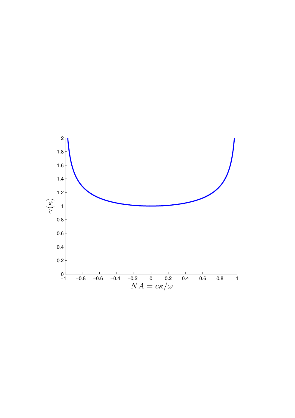
To justify the paraxial approximation, consider Fig. 3, which plots with respect to the normalized parameter , defined as the numerical aperture goodman. One can see that is relatively flat and for a wide range of . Even for an as high as , is only approximately , so in most practical cases, provides only a qualitatively unimportant correction factor.
In the paraxial regime, defined in Eq. (30) becomes the familiar -dimensional Fourier transform of ,
| (59) |
because and . is then approximately normalized,
| (60) |
can thus be roughly regarded as the configuration-space probability density of finding photons near positions respectively. Provided that we do not localize them too precisely, photons as particles in space are hence an acceptable concept in the paraxial regime and described by a properly normalized probability density.
The configuration-space model has been successfully applied to the quantum theory of optical solitons lai, where the slowly varying temporal envelope approximation holds, so it is perhaps not surprising that the model can also be applied to the spatial paraxial domain, where the optical beam is relatively uniform.
IV.1 Simple Model of Multiphoton Absorption

This probabilistic spatial interpretation of photons also provides an intuitive understanding of the expression for the multiphoton absorption rate in Eq. (35). Consider a toy model for an -photon absorption material consisting of individual -photon absorbers, each occupying a width of , as depicted in Fig. 4. The probability of all photons hitting the th absorber situated at , thus exciting an -photon absorption event at this absorber, is given by
| (61) |
where is the probability density of the -photon absorption event. The spatial resolution of the -photon absorption pattern evidently depends on . To eliminate this dependence and make the resolution depend solely on the resolution of the optical fields, we shall make very small,
| (62) |
so that in the limit of a continuous -photon absorption material, the probability density of -photon absorption becomes
| (63) |
which is proportional to given by Eq.(35). So, intuitively, an -photon absorption event occurs when all photons arrive within a very small neighborhood, and the multiphoton absorption pattern is therefore approximately given by the conditional probability distribution when all photons arrive at the same place. This model has been used by Steuernagel to approximate a four-photon absorption material by four discrete detectors steuernagel, although the explicit derivation here by the use of a configuration space model confirms the intuition that a multiphoton absorption event occurs when all photons arrive within a small neighborhood.
It must be stressed that although the interpretation of as a configuration-space probability density is only valid in the paraxial regime, the expression Eq. (35) is always a valid description of an ideal multiphoton absorption process, because of its dependence on the optical intensity, a physically measurable quantity.
IV.2 Analysis of Proof-of-Concept Experiment by D’Angelo et al.
The proof-of-concept quantum lithography experiment by D’Angelo et al. dangelo remains well within the paraxial regime, so an explicit analysis of the results can be carried out relatively easily. In this section, I shall show that the coincidence rate detected by in D’Angelo et al.’s experiment is necessarily reduced, in order to emulate quantum lithography accurately.

In the experiment depicted by Fig. 5, the spontaneously generated photon pair has the following quantum state,
| (64) |
where depends on the efficiency of the spontaneous parametric down conversion process, and must remain , so that the quantum state contains only zero or two photons in most cases. In D’Angelo et al.’s analysis, the photon pair immediately exiting the crystal is assumed to have perfect anti-correlation in transverse momentum,
| (65) |
as the pump beam is assumed to be relatively uniform across the transverse plane of the crystal and the crystal is relatively short. The spatial biphoton amplitude becomes
| (66) |
and the photons are assumed to be perfectly correlated in space. Clearly, both Eq. (65) and Eq. (66) are approximations. In any case, we shall first follow the approximate analysis and normalize the expressions later. Immediately after exiting the crystal, the photon pair passes through two slits of width spaced apart, resulting in a spatial amplitude
| (67) | ||||
| (68) |
Because the photons are assumed to be perfectly correlated in space, they always pass through the same slit, resulting in a NOON state in the spatial domain. The momentum-space amplitude, on the other hand, is given by
| (69) |
This is obviously not the NOON state in the momentum space for quantum lithography. To emulate quantum lithography indirectly, D’Angelo et al. then let the photons propagate to the far field. Via Fraunhofer diffraction goodman, the angular two-photon coincidence distribution, dangelo_note, becomes the magnitude squared of the Fourier transform of , or
| (70) | ||||
| (71) |
This expression is the same as that derived in Ref. dangelo. is now regarded as the total probability of two photons reaching the detection plane. To be more rigorous, however, in Eq. (68) and in Eq. (69) need to be normalized. For example, the delta function in Eq. (68) should be replaced by a sharp normalizable function,
| (72) |
where is a function of a dimensionless parameter and is normalized according to . is defined as the biphoton coherence length, which depends on the phase matching condition of the parametric down conversion process and the nonlinear crystal length. is assumed to be much smaller than and , but must still be non-zero in reality. The normalized then becomes
| (73) |
and the normalized becomes
| (74) |
where
| (75) |
is the dimensionless Fourier transform of . The angular distribution is hence
| (76) |
which is proportional to . Thus, in order to produce a NOON state in the near field and emulate quantum lithography accurately in the far field, the photons need to pass through the same slit, the biphoton coherence length needs to be small and is even assumed to be zero in the analysis by D’Angelo et al., but then the coincidence rate, proportional to the biphoton coherence length, is necessarily reduced.
IV.3 Jointly Gaussian Multiphoton State
In Sec. III, we have studied the use of NOON state for quantum lithography, and it has been shown that the NOON state has a lower multiphoton absorption rate than a classical state. In Sec. IV.2, we have also seen that, in order to approximate a NOON state accurately in D’Angelo et al.’s experiment, the multiphoton absorption rate is necessarily reduced. While these results provide evidence that it is probably impractical to use a NOON state for multiphoton lithography, the NOON state is only one example of infinitely many possible quantum states for optical fields, and other quantum states might be able to perform better while still producing an enhanced resolution. For example, instead of producing enhanced interference fringes with a minimum period on the order of , Björk et al. bjork considered another special quantum state, called the reciprocal binomial state, in order to produce a sharp interference spot, with a minimum width on the order of , within a periodic pattern. Still, it remains a question whether this state can produce a significantly better multiphoton absorption rate, as the NOON state is still a significant component of the reciprocal binomial state. Steuernagel, in particular, studied the four-photon reciprocal binomial state, with four discrete detectors approximating an ideal four-photon absorption material, and found that the multiphoton absorption rate is worse than that of a classical state steuernagel.
In this section, I shall study an arguably simpler and more intuitive -photon state that produces a quantum-enhanced Gaussian multiphoton absorption spot, in the paraxial regime. I shall call this state a jointly Gaussian state, which is a quantum generalization of the well known classical Gaussian beams and is able to account for quantum correlations of the photons. It is shown that, in certain limits, the jointly Gaussian state is also able to reduce the size of the multiphoton absorption spot by a factor of compared with the one photon case, but the reduction of size is always accompanied by a reduced multiphoton absorption rate. For the jointly Gaussian state, the quantum correlations of the photons, the size of the multiphoton absorption spot, as well as the absorption rate can all be adjusted by changing just two parameters, so a study of this state is able to quantify and elucidate the trade-off between resolution enhancement and multiphoton absorption rate.
IV.3.1 Many-Body Coordinate System
Before defining a jointly Gaussian state, I shall first take a detour and define a new many-body coordinate system, widely used in many-body physics, which will significantly simplify the analysis later. This coordinate transformation is
| (77) |
where is the average momentum, and is relative momentum. and of the ’s form a complete basis, so I shall somewhat arbitrarily define as the extraneous linearly dependent variable,
| (78) |
The new differential is
| (79) |
so a new multiphoton amplitude should be defined as
| (80) |
and normalized as
| (81) |
The multiphoton absorption rate in terms of the new amplitude in the paraxial approximation is
| (82) |
The multiphoton absorption rate is therefore the magnitude squared of the one-dimensional Fourier transform of , with respect to only the total momentum .
IV.3.2 -Photon Absorption of a Jointly Gaussian State
In terms of the new coordinate system, we can now define the jointly Gaussian state as follows,
| (83) |
where and are two parameters assumed to be real for simplicity, is the normalization constant,
| (84) |
as derived in Appendix B.1. This definition is inspired by the well known jointly Gaussian distribution in statistics garcia. The form of Eq. (83) is much simpler than a general jointly Gaussian distribution because of bosonic symmetry, as discussed in Appendix B.2. The momentum amplitude of the state given by Eq. (83) is also very close to that of a soliton state lai, so one can obtain a general jointly Gaussian state approximately by adiabatic control of spatial solitons fini.
The covariances of and are calculated in Appendix B.3,
| (85) |
so is a measure of the spread in the average momentum, and is a measure of the spread in the momentum relative to the average.
The variance of , the momentum of each photon in the original coordinates, is also derived in Appendix B.4 and given by
| (86) |
must be smaller than , otherwise would become imaginary, and must be much smaller than for the paraxial approximation to hold. Moreover, if an optical system has a certain aperture, it would also limit the transverse spatial frequency goodman. Hence the variance of , , must be limited, and there exists a trade-off between and .
The multiphoton absorption pattern of the jointly Gaussian state can be determined using Eq. (82),
| (87) |
The pattern is a Gaussian, with a root-mean-square width given by
| (88) |
First, consider the case in which the photons are uncorrelated, and the classical Gaussian state in the original system of coordinates is given by a product of one-photon Gaussian amplitudes,
| (89) |
As shown in Appendix B.4, this corresponds to the jointly Gaussian state when
| (90) |
The classical variance of the average momentum is equal to the variance of each momentum, , divided by . This is consistent with the statistics of independent photons. The multiphoton absorption width becomes
| (91) |
where the subscript denotes the value for a classical state. Equation (91) can be regarded as the standard quantum limit, and is better than the one-photon case by a factor of . On the other hand, the minimum width is obtained when we maximize so that and let be zero,
| (92) |
The factor-of- enhancement compared with one-photon absorption, or the factor-of- enhancement compared with classical -photon absorption, can be regarded as the ultimate quantum limit, and is consistent with other quantum enhancement schemes giovannetti. This enhancement, however, comes with a heavy price. Equation (87) shows that the multiphoton absorption rate is proportional to , so while increasing and reducing makes the Gaussian pattern sharper, the reduction in also reduces the multiphoton absorption rate, more so for large .
To quantify this trade-off, we shall fix as a given resource, and define a spot size reduction factor with respect to the classical case,
| (93) |
so that corresponds to the standard quantum limit, and corresponds to the ultimate quantum limit. We shall also define a normalized peak absorption rate with respect to the rate in the classical case,
| (94) |

Figure 6 plots versus for several values of . This result is decidedly disappointing, as it shows that the maximum multiphoton absorption rate is obtained when the state is a classical state, or , and the peak rate monotonically decreases to zero as the spot size is reduced. Furthermore, even if one is willing to sacrifice the resolution and increase , the peak absorption rate is still reduced, because of its dependence on .
For applications such as multiphoton spectroscopy, spatial resolution is not important, and it is more desirable to maximize the total multiphoton absorption rate. We can define the normalized total rate as
| (95) |

Figure 7 plots versus . It can be seen that the total rate does increase when one increases the spot size, but the rate enhancement is very moderate. In fact, in the limit of , approaches
| (96) |
so the ultimate rate enhancement, when resolution is completely sacrificed and , asymptotically approaches for large . This small enhancement of multiphoton absorption rate is not likely to be useful.
To understand the above results, it is helpful to consider the position correlation of the photons, derived in Appendix B.5,
| (97) |
To obtain an enhanced multiphoton resolution, the bandwidth of the average momentum, , must be increased, leading to a positive correlation in the momenta and a negative correlation in the positions of the photons. So the photons are actually less likely to arrive near one another, leading to a lower probability of the photons hitting the same absorber and therefore a correspondingly less multiphoton absorption rate. On the other hand, if is reduced, the position correlation becomes positive, and the photons are more likely to arrive close to one another, leading to a slightly enhanced total absorption rate. Ultimately, how close the photons can arrive with respect to one another is still restricted by the resolution limit of the optical system, so the rate enhancement is not significant.
It must be stressed again that the preceding argument, as well as Boto et al.’s heuristic argument about photons constrained to arrive at the same place, are only applicable to the paraxial regime, where the positions of photons are relatively well defined quantities. The example of the jointly Gaussian state shows that, even in the paraxial regime, Boto et al.’s heuristic argument is not correct, and the photons are actually less likely to “arrive at the same place” when the resolution is enhanced. Although this has been shown by Steuernagel for the specific example of four-photon reciprocal binomial state steuernagel, the study of joint Gaussian state here confirms this fact for an arbitrary number of photons.
V Discussion and Conclusion
In summary, through a rigorous study of quantum lithography and the NOON state, an investigation of the proof-of-concept experiment by D’Angelo et al.dangelo, and an analysis of a jointly Gaussian state, I have been unable to find any evidence, as far as the spatial domain is concerned, that supports the heuristic claim by Boto et al. boto, namely that the photons would be “constrained to arrive at the same place” and the multiphoton absorption rate would be enhanced due to spatial effects. On the contrary, all examples show that the multiphoton absorption rate is actually reduced, more so for larger , when a quantum state is used to enhance the resolution.
Admittedly, there are several assumptions involved in the analysis, the negligence of time domain effects in particular. As Javanainen and Gould javanainen and Perina et al. perina have shown, frequency entanglement can enhance the multiphoton absorption rate, but this enhancement is likely to be independent of the detrimental spatial effect, which seems to be an unavoidable penalty incurred by the resolution enhancement effect itself. That said, it remains to be proved whether taking time domain into account would be able to eliminate or reverse the detrimental spatial effect.
Moreover, only the NOON state and the jointly Gaussian state have been studied in this paper, but the possibility of other exotic quantum states being able to enhance the resolution while maintaining a respectable multiphoton absorption rate cannot be ruled out. In fact, alternative strategies have already been proposed to solve the low exposure problem of quantum lithography. For example, Agarwal et al. have shown that strong nonclassical beams from a parametric amplifier can also produce enhanced two-photon interference fringes agarwal, albeit with a background worse than a classical multiple exposure technique bentley. Hemmer et al. also proposed the use of a narrowband multiphoton absorption material and classical light hemmer, similar to Yablonovitch and Vrijen’s proposal yablonovitch, to achieve the same resolution enhancement as quantum lithography.
In conclusion, in light of the results set forth, the original quantum lithography scheme is unlikely to be practical in the near future. Nonetheless, it has inspired many ongoing research efforts on the elusive goal of beating the optical resolution limit, and should therefore remain an interesting theoretical concept.
Discussions with Demetri Psaltis, Robert W. Boyd, Jonathan P. Dowling, Bahaa E. A. Saleh, and Paul W. Kwiat are gratefully acknowledged. This work is financially supported by DARPA and the National Science Foundation through the Center for the Science and Engineering of Materials (DMR-0520565).
Appendix A Physical Significance of the Geometric Factor
To understand why the factor arises in Eq. (30) of the formalism, consider the electric field envelope given by Eq. (19),
| (98) |
where is the dependent variable given by . We shall leave the form of unspecified and derive it purely from the fact that the formalism is invariant under a rotation in the plane. Imagine that the electric field profile is rotated anticlockwise in the plane, where is the horizontal axis and is the vertical axis, by an angle . This is equivalent to defining new coordinates as follows,
| (99) |
The envelope becomes
| (100) | ||||
| (101) |
If we define the momenta in the new coordinate system to be
| (102) |
evidently the new definitions still satisfy the dispersion relation
| (103) |
More crucially, the coordinate transformation yields
| (104) |
so that the electric field envelope becomes
| (105) |
If the electric field is invariant to such a rotation, we should be able to define a new momentum-space operator such that
| (106) |
with the commutator
| (107) |
Comparing Eq. (105) and Eq. (106), we have
| (108) |
but the coordinate transformation also restricts the relation between and ,
| (109) |
Combining Eq. (108) and Eq. (109) yields
| (110) |
For Eq. (110) to hold for any rotation, must depend on only according to the following,
| (111) |
where is an arbitrary constant. Equation (111) is identical to Eq. (21) with . Hence, the factor arises purely due to the invariance of the formalism with respect to rotation in the plane. Furthermore, the general transformation rule for with respect to a rotation is given by Eq. (108), or
| (112) | ||||
| (113) |
Appendix B Properties of the Jointly Gaussian State
In this section I shall derive several properties of the jointly gaussian state,
| (114) |
where is the normalization constant, and are real parameters, and is given by .
B.1 Normalization
B.2 Bosonic Symmetry
I shall now show that Eq. (114) is a consequence of enforcing bosonic symmetry on a general jointly Gaussian function. In the original coordinate system, can be determined from Eq. (80),
| (120) |
which can be rewritten as
| (121) |
Equation (121) is a general jointly Gaussian function, but because of boson symmetry of as prescribed by Eq. (28), must have identical on-axis components, as well as identical off-axis components. With some algebra, can be determined from Eq. (120),
| (122) | ||||
| (123) |
Any with identical on-axis components and identical off-axis components can be specified using and , so Eq. (114) can specify any general jointly Gaussian functions with bosonic symmetry.
B.3 Covariances
The covariances of momentum variables should be determined from the probability distribution
| (124) |
where is defined in Appendix B.1. The variance of is simply given by
| (125) |
while the covariance matrix for ’s is given by
| (126) |
Because only has two parameters, its inverse, defined as , is easy to calculate and is given by
| (127) |
We thus obtain the covariances,
| (128) |
B.4 Classical Gaussian State
The covariances of in the original coordinate system are
| (129) | ||||
| (130) | ||||
| (131) |
So the photons are uncorrelated when , and in Eq. (121) can be written as
| (132) |
a product of one-photon Gaussian amplitudes, and therefore a classical state.
B.5 Configuration-Space Multiphoton Amplitude
In the paraxial regime, the configuration-space multiphoton amplitude can be obtained by Fourier transform of Eq. (121),
| (133) |
which is determined using the well known characteristic function of a jointly Gaussian distribution garcia. The configuration-space probability density is thus
| (134) |
and the covariance matrix for the photon positions is . The position variance is then
| (135) |
and the covariance is
| (136) |
References
- (1) M. Born and E. Wolf, Principles of Optics (Cambridge University Press, Cambridge, 1999).
- (2) C. W. Gwyn, R. Stulen, D. Sweeney, and D. Attwood, J. Vac. Sci. Technol. B 16, 3142 (1998).
- (3) E. Yablonovitch and R. B. Vrijen, Opt. Eng. 38, 334 (1999).
- (4) A. N. Boto, P. Kok, D. S. Abrams, S. L. Braunstein, C. P. Williams, and J. P. Dowling, Phys. Rev. Lett. 85, 2733 (2000).
- (5) G. S. Agarwal, R. W. Boyd, E. M. Nagasako, and S. J. Bentley, Phys. Rev. Lett. 86, 1389 (2001); E. M. Nagasako, S. J. Bentley, R. W. Boyd, G. S. Agarwal, Phys. Rev. A64, 043802 (2001).
- (6) S. J. Bentley and R. W. Boyd, Opt. Express 12, 5735 (2004).
- (7) P. R. Hemmer, A. Muthukrishnan, M. O. Scully, and M. S. Zubairy, Phys. Rev. Lett. 96, 163603 (2006).
- (8) R. W. Boyd and S. J. Bentley, J. Mod. Opt. 53, 713 (2006), and references therein.
- (9) J. Javanainen and P. L. Gould, Phys. Rev. A41, 5088 (1990).
- (10) J. Perina, Jr., B. E. A. Saleh, and M. C. Teich, Phys. Rev. A57, 3972 (1998).
- (11) O. Steuernagel, J. Opt. B 6, S606 (2004).
- (12) L. Mandel and E. Wolf, Optical Coherence and Quantum Optics (Cambridge University Press, Cambridge, 1995).
- (13) M. D’Angelo, M. V. Chekhova, and Y. Shih, Phys. Rev. Lett. 87, 013602 (2001).
- (14) K. J. Blow, R. Loudon, S. J. D. Phoenix, and T. J. Shepherd, Phys. Rev. A42, 4102 (1990); see also B. Huttner and S. M. Barnett, Phys. Rev. A46, 4306 (1992).
- (15) H. P. Yuen and J. H. Shapiro, IEEE Trans. Inf. Theory IT-24, 657, (1978).
- (16) Notice that Ref. yuen incorrectly assumes .
- (17) S. S. Schweber, An Introduction to Relativistic Quantum Field Theory (Row, Peterson and Company, New York, 1961).
- (18) J. W. Goodman, Introduction to Fourier Optics (McGraw-Hill, Boston, 1996).
- (19) Y. Lai and H. A. Haus, Phys. Rev. A40, 844 (1989); 40, 854 (1989); Hagelstein ibid. 54, 2426 (1996).
- (20) In D’Angelo et al.’s experiment, the two photons are actually orthogonally polarized, and the measured quantity is , where the subscripts and denote different polarizations. This measurement is the same as the two-photon absorption pattern if the two photons had the same polarization, so we shall neglect this subtlety and use the expression for simplicity.
- (21) G. Björk, L. L. Sánchez-Soto, and J. Söderholm, Phys. Rev. Lett. 86, 4516 (2001).
- (22) A. Leon-Garcia, Probability and Random Processes for Electrical Engineering (Addison-Wesley, Reading, 1994).
- (23) J. M. Fini and P. L. Hagelstein, Phys. Rev. A66, 033818 (2002); M. Tsang, Phys. Rev. Lett. 97, 023902 (2006).
- (24) V. Giovannetti, S. Lloyd, and L. Maccone, Science 306, 1330 (2004).