Analysis of entropy of $XY$ Spin Chain

F. Franchini

\diamond

A. R. Its† B.-Q. Jin§ V. E. Korepin

\star

Affiliation:

\star

C.N. Yang Institute for Theoretical Physics, State University of New York at Stony Brook, Stony Brook, NY 11794-3840, USA Email: Fabio.Franchini@stonybrook.edu,itsa@math.iupui.edu,jinbq@wzu.edu.cn, korepin@insti.physics.sunysb.edu

Abstract

Entanglement in the ground state of the $XY$ model on the infinite chain can be measured by the von Neumann entropy of a block of neighboring spins. We study a double scaling limit: the size of the block is much larger then $1$ but much smaller then the length of the whole chain. In this limit, the entropy of the block approaches a constant. The limiting entropy is a function of the anisotropy and of the magnetic field. The entropy reaches minima at product states and increases boundlessly at phase transitions.

pacs

03.65.Ud, 02.30.Ik, 05.30.Ch, 05.50.+q

1 Introduction

Entanglement is a primary resource for quantum computation and information processing [1, 2, 3, 4]. It shows how much quantum effects we can use to control one system by another. Stable and large scale entanglement is necessary for scalability of quantum computation [5, 6]. The entropy of a subsystem as a measure of entanglement was discovered in [3]. Essential progress has been achieved in the understanding of entanglement in various quantum systems [5, 7, 8, 9, 10, 37, 11, 12, 13, 14, 15, 17, 18, 19].

The importance of the $XY$ model for quantum information was emphasized in [7, 20, 21, 22]. In this paper we consider the entropy of a block of $L$ neighboring spins in the ground state of the $XY$ model [on the infinite chain] in the limit $L\rightarrow\infty$ . We use the results of [23, 24, 25]. The Hamiltonian of the $XY$ model is

{\cal H}=-\sum_{n=-\infty}^{\infty}(1+\gamma)\sigma^{x}_{n}\sigma^{x}_{n+1}+(1-\gamma)\sigma^{y}_{n}\sigma^{y}_{n+1}+h\sigma^{z}_{n}

(1)

Here $0<\gamma<1$ is the anisotropy parameter; $\sigma^{x}_{n}$ , $\sigma^{y}_{n}$ and $\sigma^{z}_{n}$ are the Pauli matrices and $0<h$ is the magnetic field. The model was solved in [26, 27, 28, 29]. The methods of Toeplitz determinants and integrable Fredholm operators were used for the evaluation of correlation functions, see [28, 30, 31, 32, 33, 34]. The idea to use the determinants for calculation of entropy was put forward in [8].

Solution of $XY$ looks differently in three cases: $\Downarrow$

Case $1$ a is defined by the inequality $\quad 2\sqrt{1-\gamma^{2}}<h<2$ .

It describes moderate magnetic field.

Case $2$ is defined by $h>2$ . This is strong magnetic field.

Case $1$ b is defined by $0<h<2\sqrt{1-\gamma^{2}}$ .

It is weak magnetic field, including zero magnetic field.

At the boundary between cases $1$ a and $1$ b ( $h=2{\sqrt{1-\gamma^{2}}}$ ) the ground state is doubly degenerated:

	$\displaystyle\|G_{1}\rangle$	$\displaystyle=$	$\displaystyle\prod_{n\in\mbox{\rm lattice}}\left[\cos(\theta)\|\uparrow_{n}\rangle+(-1)^{n}\sin(\theta)\|\downarrow_{n}\rangle\right],\qquad\qquad\qquad\bowtie$
	$\displaystyle\|G_{2}\rangle$	$\displaystyle=$	$\displaystyle\prod_{n\in\mbox{\rm lattice}}\left[\cos(\theta)\|\uparrow_{n}\rangle-(-1)^{n}\sin(\theta)\|\downarrow_{n}\rangle\right]$		(2)

Here $\cos^{2}(2\theta)=(1-\gamma)/(1+\gamma)$ . The role of factorized states was emphasized in [30, 35, 36]. Let us mention that the rest of energy levels are separated by a gap and correlations decay exponentially. The boundary boundary between cases $1$ a and $1$ b is not a phase transition.

In general, we denote the ground state of the model by $|GS\rangle$ . We consider the entropy of a block of $L$ neighboring spins: it measures the entanglement between the block and the rest of the chain [3, 20]. We treat the whole ground state as a binary system $|GS\rangle=|A\&B\rangle$ . The block of $L$ neighboring spins is subsystem A and the rest of the ground state is subsystem B. The density matrix of the ground state is $\rho_{AB}=|GS\rangle\langle GS|$ . The density matrix of the block is $\rho_{A}=Tr_{B}(\rho_{AB})$ . The entropy $S(\rho_{A})$ of the block is:

S(\rho_{A})=-Tr_{A}(\rho_{A}\ln\rho_{A})\qquad\qquad\qquad\sharp

(3)

Note that each of the ground states (2) is factorized and has no entropy.

To express the entropy we need the complete elliptic integral of the first kind,

I(k)=\int_{0}^{1}\frac{dx}{\sqrt{(1-x^{2})(1-k^{2}x^{2})}}\qquad\qquad\star

and the modulus

\tau_{0}=I(k^{\prime})/I(k),\qquad\qquad k^{\prime}=\sqrt{1-k^{2}}

(4)

In the paper [23] we used determinant representation for evaluation of entropy. Zeros of the determinant form an infinite sequence of numbers:

\lambda_{m}=\tanh\left(m+\frac{1-\sigma}{2}\right)\pi\tau_{0},\quad m\geq 0,\qquad\lambda_{-m}=-\lambda_{m}

(5)

here $\sigma=1$ in Case 1 and $\sigma=0$ in Case 2. Note $0<\lambda_{m}<1$ and $\lambda_{m}\to 1$ as $m\to\infty$

The magnetic field and anisotropy define $k$ :

\displaystyle k=\left\{\begin{array}[]{c}\sqrt{(h/2)^{2}+\gamma^{2}-1}\;/\;\gamma,\;\;\;\qquad\qquad\mbox{Case 1a}\\[8.5359pt] \sqrt{1-\gamma^{2}-(h/2)^{2}}\;/\;\sqrt{1-(h/2)^{2}},\;\;\;\mbox{Case 1b}\\[8.5359pt] \gamma\;/\;\sqrt{(h/2)^{2}+\gamma^{2}-1},\;\;\;\qquad\qquad\mbox{Case 2}\end{array}\right.

We represented the entropy as a convergent series in [23]:

\heartsuit\quad\qquad S(\rho_{A})=\sum_{m=-\infty}^{\infty}(1+\lambda_{m})\ln\frac{2}{1+\lambda_{m}}\qquad\spadesuit

(10)

I. Peshel using the approach of [11] also obtained the series (10) in cases of non-zero magnetic field, see [24]. He summed it up into:

S(\rho_{A})=\frac{1}{6}\left[\;\ln{\left(\frac{k^{2}}{16k^{\prime}}\right)}+\left(1-\frac{k^{2}}{2}\right)\frac{4I(k)I(k^{\prime})}{\pi}\right]+\ln\;2,\qquad{\mbox{ Case 1a}}

S(\rho_{A})=\frac{1}{12}\left[\;\ln{\frac{16}{(k^{2}k^{\prime 2})}}+(k^{2}-k^{\prime 2})\frac{4I(k)I(k^{\prime})}{\pi}\right],\qquad\qquad\quad{\mbox{ Case 2}}

We summed up the series (10) in case of weak magnetic field (including zero magnetic field) in the paper [23]:

\clubsuit\qquad S(\rho_{A})=\frac{1}{6}\left[\;\ln{\left(\frac{k^{2}}{16k^{\prime}}\right)}+\left(1-\frac{k^{2}}{2}\right)\frac{4I(k)I(k^{\prime})}{\pi}\right]+\ln\;2,\qquad\mbox{ Case 1b},

The rigorous proof and the precise history is given in the paper [25].

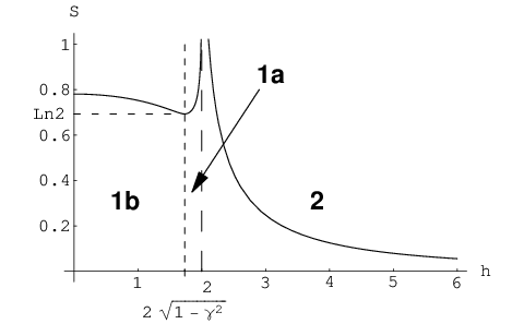
Refer to caption — Figure 1: The limiting entropy as a function of the magnetic field at constant anisotropy $\gamma=1/2$ . The entropy has a local minimum $S=\ln 2$ at $h=2\sqrt{1-\gamma^{2}}$ and the absolute minimum for $h\to\infty$ where it vanishes. $S$ is singular at the phase transition $h=2$ where it diverges to $+\infty$ . The three cases are marked.

Now we can study the range of variation of the limiting entropy. We find a local minimum $S(\rho_{A})=\ln 2$ at the boundary between cases $1$ a and $1$ b ( $h=2\sqrt{1-\gamma^{2}}$ ). This is the case of double degenerated ground state (2). The absolute minimum is achieved at infinite magnetic field, where the ground state becomes ferromagnetic (i.e. all spins are parallel). The entropy diverges to $+\infty$ , i.e has singularities, at the phase transitions: $h=2$ [11] or $\gamma=0$ , see [8]. To show this behavior of the limiting entropy, we plot it as a function of the magnetic field $h$ at constant anisotropy $\gamma=1/2$ in Fig. 1. It is interesting to note that the critical behavior of the $XY$ model is similar to the Lipkin-Meshkov-Glick model [37].

Acknowledgments. We would like to thank P.Deift, B.McCoy, I.Peschel and H.Widom for useful discussions. This work was supported by NSF Grants DMR-0302758, DMS-0099812 and DMS-0503712.

References

[1] C.H. Bennett, D.P. DiVincenzo, Nature 404, 247 (2000)
[2] S. Lloyd, Science 261,1569 (1993); ibid 263,695 (1994).
[3] C.H. Bennett, H.J. Bernstein, S. Popescu, and B. Schumacher, Phys. Rev. A 53, 2046 (1996)
[4] S. Popescu, A. J. Short, A. Winter, quant-ph/0511225
[5] P. Zanardi, M. Rasetti, Phys. Lett. A 264, 94 (1999); A. Marzuoli, M. Rasetti, Phys. Lett. A 306, 79 (2002); M. Rasetti, cond-mat/0211081
[6] V.Vedral, Nature 425, 28 (2003), New J. Phys. 6,10 (2004)
[7] A. Osterloh, L. Amico, G. Falci and R. Fazio, Nature 416 608 (2002)
[8] B.-Q. Jin, V. E. Korepin, J. Stat. Phys. 116, 79 (2004)
[9] J.I. Latorre, E. Rico, G. Vidal, QIC. 4, 048 (2004)
[10] V.E.Korepin, Phys.Rev. Lett. 92, 096402 (2004)
[11] P. Calabrese, J. Cardy, JSTAT 0406, P002 (2004)
[12] M.C.Arnesen, S.Bose, V.Vedral, Phys. Rev. Lett. 87, 017901 (2001)
[13] F. Verstraete, M.A. Martín-Delgado, J.I. Cirac, Phys. Rev. Lett. 92, 087201 (2004)
[14] R. Orus, J.I. Latorre, Phys. Rev. A 69, 052308 (2004)
[15] J.K. Pachos, M.B. Plenio, Phys. Rev. Lett. 93, 056402(2004)
[16] H. Fan, V. Korepin, V. Roychowdhury, Phys. Rev. Lett. 93, 227203 (2004)
[17] M.B. Plenio, J. Eisert, J. Dreissig, M. Cramer, quant-ph/0405142
[18] S. Anders, M. B. Plenio, W. Dr, F. Verstraete, H.-J. Briegel, quant-ph/0602230
[19] S. Michalakis, B. Nachtergaele, math-ph/0606018
[20] G. Vidal, J.I. Latorre, E. Rico, A. Kitaev, Phys. Rev. Lett. 90, 227902 (2003)
[21] J.P. Keating, F. Mezzadri, Commun. Math. Phys. 252, 543 (2004)
[22] D. G. Angelakis, M. F. Santos, S. Bose, quant-ph/0606159
[23] A. R. Its, B.-Q. Jin, V. E. Korepin, J. Phys. A 38, 2975 (2005)
[24] I. Peschel, J. of Stat. Mech., P12005 (2004)
[25] A. R. Its, B.-Q. Jin, V. E. Korepin, quant-ph/0606178
[26] E. Lieb, T. Schultz and D. Mattis, Ann. Phys. 16, 407 (1961)
[27] E. Barouch and B.M. McCoy, Phys. Rev. A 3, 786 (1971)
[28] E. Barouch, B.M. McCoy and M. Dresden, Phys. Rev. A 2, 1075 (1970)
[29] D.B. Abraham, E. Barouch, G. Gallavotti and A. Martin-Löf, Phys. Rev. Lett. 25, 1449 (1970); Studies in Appl. Math. 50, 121 (1971); ibid 51, 211 (1972)
[30] A.G. Abanov, F. Franchini, Phys. Lett. A 316, 342 (2003); F. Franchini, A.G. Abanov, J. Phys. A 38 5069 (2005)
[31] A.R. Its, A.G. Izergin, V.E. Korepin, and N. A. Slavnov, Phys. Rev. Lett. 70 , 1704 (1993)
[32] P.A. Deift, X. Zhou, Plenum Press, New York and London (1994)
[33] M.B. Zvonarev, A.G. Izergin, A.G.Pronko, J. Math. Sci. (N. Y.) 115 (2003), no. 1, 2002–2008 82B20
[34] V.S. Kapitonov, A.G. Pronko, J. Math. Sci. (N. Y.) 115 (2003), no. 1, 2009–2032 (Reviewer: Anatoliy Yu. Zakharov) 82B20 (82B23)
[35] T. Roscilde, P. Verrucchi, A. Fubini, S. Haas, V. Tognetti, Phys. Rev. Lett. 94, 147208 (2005)
[36] T. Roscilde, P. Verrucchi, A. Fubini, S. Haas, V. Tognetti, quant-ph/0412056
[37] J.I. Latorre, R. Orus, E. Rico, J. Vidal, Phys. Rev. A 71, 064101 (2005); J.Vidal, R. Mosseri, J. Dukelsky, Phys. Rev. A 69, 054101 (2004); J.Vidal, G. Palacios R. Mosseri, Phys. Rev. A 69, 022107 (2004); S. Dusuel, J.Vidal, Phys. Rev. Lett. 93, 237204 (2004) and Phys. Rev. B 71, 224420 (2005); T. Barthel, S. Dusuel, J. Vidal, cond-mat/0606436

	$\displaystyle\|G_{1}\rangle$	$\displaystyle=$	$\displaystyle\prod_{n\in\mbox{\rm lattice}}\left[\cos(\theta)\|\uparrow_{n}\rangle+(-1)^{n}\sin(\theta)\|\downarrow_{n}\rangle\right],\qquad\qquad\qquad\bowtie$
	$\displaystyle\|G_{2}\rangle$	$\displaystyle=$	$\displaystyle\prod_{n\in\mbox{\rm lattice}}\left[\cos(\theta)\|\uparrow_{n}\rangle-(-1)^{n}\sin(\theta)\|\downarrow_{n}\rangle\right]$		(2)

Analysis of entropy of X​YXY Spin Chain

Abstract

pacs

1 Introduction

References

Analysis of entropy of $XY$ Spin Chain