Secrecy extraction from no-signalling correlations
Abstract
Quantum cryptography shows that one can guarantee the secrecy of correlation on the sole basis of the laws of physics, that is without limiting the computational power of the eavesdropper. The usual security proofs suppose that the authorized partners, Alice and Bob, have a perfect knowledge and control of their quantum systems and devices; for instance, they must be sure that the logical bits have been encoded in true qubits, and not in higher-dimensional systems. In this paper, we present an approach that circumvents this strong assumption. We define protocols, both for the case of bits and for generic -dimensional outcomes, in which the security is guaranteed by the very structure of the Alice-Bob correlations, under the no-signalling condition. The idea is that, if the correlations cannot be produced by shared randomness, then Eve has poor knowledge of Alice’s and Bob’s symbols. The present study assumes, on the one hand that the eavesdropper Eve performs only individual attacks (this is a limitation to be removed in further work), on the other hand that Eve can distribute any correlation compatible with the no-signalling condition (in this sense her power is greater than what quantum physics allows). Under these assumptions, we prove that the protocols defined here allow extracting secrecy from noisy correlations, when these correlations violate a Bell-type inequality by a sufficiently large amount. The region, in which secrecy extraction is possible, extends within the region of correlations achievable by measurements on entangled quantum states.
I Introduction
Quantum physics has been shown to provide a means to distribute correlations at a distance, whose secrecy can be guaranteed by the laws of physics, without any assumption on the computational power of the eavesdropper. This is the nowadays largely studied field of quantum cryptography (or quantum key distribution, QKD), the most mature development of quantum information science [1]. The fact itself, that quantum physics can be used to distribute secrecy, is safe: if the authorized partners share a maximally entangled state, then secrecy is definitely guaranteed. But of course, one must verify that secrecy is not immediately spoiled by any small departure from this ideal case; this is why much theoretical research has been devoted to the derivation of rigorous bounds for the security of quantum cryptography [2]. Still, a lot of questions remain unsolved: for instance, the theorists, who find security proofs, and the experimentalists, who realize devices, tend to make different and often incompatible assumptions when figuring their schemes out.
In particular, an assumption in theoretical proofs has gone unnoticed until recently [3, 4]: one assumes that the logical bits are encoded in quantum systems whose dimension is under perfect control (generally, qubits). Why do we question this assumption? First, because it is interesting in itself to ask, whether one can remove an assumption, that is, whether one can base the studies of security on weaker constraints. Second, because side channels are a serious issue in practical quantum cryptography. Experimentalists have to be careful that, when they encode (say) polarization, they encode only polarization, and that the device does not change the spectral line, or the spatial mode, or the temporal mode of the photon as well. Third, because it is important for practical reasons: quantum cryptography is becoming a commercial product. If a security expert recommends a quantum cryptography device, he should be able to assess that the device acts as it should with ”reasonable” means. After all, the eavesdropper Eve could be herself the provider of the device!
Anyone faced with this scenario feels at first that, if Eve is allowed to sell you the devices and you cannot know them in detail, there is no hope for security. Surprisingly, recent advances in quantum information suggest that this despair, reasonable as it is, may be too pessimistic. Let’s see where the hope lies, and which assumptions are really crucial.
The scheme to distribute correlations we have in mind is represented in Fig. 1. In Alice’s and Bob’s laboratories, the dark grey square represents the device possibly provided by Eve. The distribution of correlations is made in three steps. In the first step, both laboratories are open to the signal that correlate them. This signal comes either from outside, or is emitted by Alice’s device to Bob’s, or viceversa: in any case, it must be assumed to be under Eve’s full control. In the second step, the laboratories are completely sealed, an obviously necessary condition as we are going to see. On the device that reads the signal, Alice and Bob must have a knob, which allows them to choose among at least two alternatives (in usual QKD, this is for instance the choice of the basis). It is obviously necessary to assume that no information about the position of the knob leaks out of Alice’s and Bob’s laboratories (in QKD, if Eve would know the basis, she can measure the state without introducing errors). Now, conditioned on the choice of an input (a position of the knob, labelled for Alice and for Bob), an output is produced ( for Alice, for Bob). The lists of and constitute the raw key. How can there be some secrecy in this raw key? The insight from quantum physics is that the outputs may be not under the provider’s control: if the probability distribution of the outputs violates some kind of Bell inequality, then by definition those outputs have not been produced by shared randomness — in other words, the correlations have been produced by the measurements themselves, and did not pre-exist to them. They could have been produced by communication, if information about the inputs and/or would have propagated between Alice and Bob; but we have insisted on the no-signalling assumption: no information about and should leak out of Alice’s and Bob’s laboratories respectively [5]. The third step is usual: Alice and Bob can make classical data processing in order to distill a fully secret key.

The reasoning above is exactly the intuition that led Ekert to discover (independently of previous works) quantum cryptography in 1991 [6]. Ekert’s work contains in nuce the idea of a device-independent security proof: it should be possible to demonstrate that a probability distribution, which violates some Bell inequality, is secure by this very fact, without any reference to the formalism of quantum physics. Of course, in physics as we know it today, a Bell inequality can only be violated with entanglement: that is why people immediately used the quantum formalism to study Ekert’s intuition [7]. But recently, tools have been developed, that allow one to study no-signalling distributions in themselves, without the formalism of Hilbert spaces. It is then possible to come back to the original intuition by Ekert, and try and prove security only through the violation of a Bell-type inequality. This is the theme of the present paper.
II Cryptography in the no-signalling polytope
This first section introduces the language and the tools which are needed in a general framework. We focus from the very beginning onto bipartite correlations, i.e. correlations involving two partners, traditionally called Alice and Bob.
II.1 Formalization of Bell-type experiments
The physical situation one must keep in mind is a Bell-type experiment. Alice and Bob receive several pairs of entangled quantum particles. On each particle, Alice performs the measurement randomly drawn from a finite set of possibilities; as a result, she obtains the output out of a discrete set containing symbols. Independently from Alice, Bob performs the measurement randomly drawn from a finite set of possibilities; as a result, he obtains the output out of a discrete set containing symbols. Such an experiment is characterized by the family of probabilities
| (1) |
There are such numbers, so each experiment can be described by a point in a -dimensional space; more precisely, in a region of such a space, bounded by the conditions that probabilities must be positive and sum up to one. By imposing further restrictions on the possible probability distributions, the region of possible experiment shrinks, thus adding non-trivial boundaries [8, 9, 10]. For our study, three restrictions are meaningful.
The first restriction is the requirement that the probability distribution must be built without communication, only with shared randomness. In the literature, this has been known as the hypothesis of local hidden variables. In our context, these variables are not hidden ”in nature” (as in the original interpretational debates about quantum physics): they may rather be hidden in Alice’s and Bob’s laboratories, in the devices that Eve has provided to them. The bounded region, which contains all probability distributions that can be obtained by shared randomness, forms a polytope, that is a convex set bounded by a finite number of hyperplanes (”facets”); therefore we refer to it as to the local polytope. The vertices of the local polytope are the points corresponding to deterministic strategies, that is, strategies in which and with probability one; that is, . There are clearly such strategies. The vertices are thus easily listed, but to find the facets given the vertices is a computationally hard task. The importance of finding the facets is pretty clear. If a point, representing an experiment, lies within the polytope, then there exists a strategy with shared randomness (a local variable model) that produces the same probability distribution. If on the contrary a point lies outside the local polytope, then the experiment cannot be reproduced with shared randomness only. The interpretation of the facets of the local polytope is therefore obvious: they correspond to Bell’s inequalities. We shall call non-local region the region which lies outside the local polytope.
The second restriction is the requirement that the probability distribution must be obtained from measurements on quantum bipartite systems. The bounded region thus obtained shall be called the quantum region. It is not a polytope, since there is not a finite set of extremal points. It is a convex set if one really allows all possible measurements on all possible states in arbitrary-dimensional Hilbert space [9, 11]; if one restricts to the measurements on a given state, or even to von-Neumann measurements on a Hilbert space with given dimension, convexity is not proved in general (although no counter-example is known, to our knowledge). Needless to recall, the quantum region contains the local polytope, but is larger than it: measurement on quantum states can give rise to non-local correlations (Bell inequalities are violated).
The third restriction is the requirement that the probability distribution must not allow signalling from Alice to Bob or viceversa. The no-signalling requirement is fulfilled if and only if Alice’s marginal distribution does not depend on Bob’s choice of input, and viceversa: that is, the probability distributions must fulfill
| (2) | |||||
| (3) |
These conditions define again a polytope, the no-signalling polytope, which contains the quantum region. The deterministic strategies are still vertices for this polytope; to these, one must add other vertices which represent, loosely speaking, purely non-local no-signalling strategies. These additional points, sometimes called non-local machines or non-local boxes, have been fully characterized only in a few cases.
II.2 Secrecy of probability distributions
Here is the question that we are going to address in this paper. Alice and Bob have repeated many times the ”measurement” procedure and share an arbitrary large number of realizations of the random variables distributed according to . By revealing a fraction of their lists, they can estimate whether their probability distribution lies in the local polytope or in the non-local region. The goal is to study whether Alice and Bob can extract secrecy out of their data with this knowledge only.
To motivate the question, let us consider the best-known quantum cryptography protocol, the one invented by Bennett and Brassard in 1984 (BB84) [12]. In this protocol, and are both binary. In the absence of any error, the BB84 protocol distributes perfect correlations when and no correlations when , that is: , , and . If Alice and Bob have obtained their results by measuring two-dimensional quantum systems (qubits), such correlations provide secrecy under the usual assumption that the eavesdropper is limited only by the laws of quantum physics [13]. However, this distribution can also be obtained with shared randomness: if Alice and Bob would share randomly distributed pairs of classical bits , they simply have to output (respectively ) if they are asked to measure (respectively ). Thus we see the importance of the additional assumption on the physical realization, namely, that both Alice and Bob are measuring a qubit, and therefore the pair is not available because .
In other words, the correlations of BB84, even in the absence of errors, are not secure ”by themselves”: they are secure only provided the quantum degrees of freedom are under good control. The question we raised can now be put in its true perspective: are there correlations that are secure by themselves, by the very fact of being what they are, without having even to describe how Alice and Bob managed to obtain them from a real channel?
It turns out that it is easier to tackle this question by considering that the eavesdropper Eve is not even limited by quantum physics, but only by the no-signalling constraint. This means that Eve can distribute any many-instances probability distribution that lies within the no-signalling polytope; Alice and Bob have the freedom of choosing their sequence of measurements ( and respectively) and will obtain the corresponding outcomes. By making this assumption, we stand clearly on the conservative side: if we can demonstrate that a non-vanishing secret key can be extracted against such a powerful eavesdropper, then the secret key achievable against a ”realistic” (i.e., quantum) eavesdropper will be at least as long.
In quantum cryptography, secrecy relies on entanglement. On which physical quantity can such a strong security, as the one we are asking for, rely? The answer is: on the non-locality of the correlations, that is, on the fact that the correlations cannot be obtained by shared randomness [5]. No secrecy can be extracted if Alice and Bob share a probability distribution which lies within the local polytope, just as no secrecy against a quantum Eve can be extracted out of separable states [14, 15].
II.3 Individual eavesdropping strategies
Barrett, Hardy and Kent [3] have shown an example of a protocol, in which quantum correlations can provide secrecy against the most powerful attack by a no-signalling Eve. This is the first example that one can achieve security even against a supra-quantum Eve, showing that security in key distribution arises from general features of no-signalling distributions rather than from the specificities of the Hilbert space structure. However, their example has important limitations: actually, it provides a protocol to distribute a single secret bit (thence zero key rate) in the case when Alice and Bob share correlations that can be ascribed to noiseless quantum states.
In this paper, we tackle the problem from the other side: we don’t go straight for security against the most powerful adversary, but we follow the same path that was followed historically by quantum cryptography, namely, we limit the eavesdropper to adopt an individual strategy. This means the following: Eve follows the same procedure for each instance of measurement — that is, she is not allowed to correlate different instances. Moreover, Eve is asked to put her input before any error correction and privacy amplification. Consequently, any individual attack is described of a three-partite probability distribution such that
| (4) |
Note that Eve is also limited by no-signalling, that is why the left hand side does not depend on . One can see that this is an individual attack by looking at it as follows: when Eve gets outcome out of her input , she sends out the point .
Now we demonstrate two similar, important results about individual eavesdropping strategies:
Theorem 1: Eve can limit herself in sending out extremal points of the no-signalling polytope.
Proof. Suppose that an attack is defined, in which one of the is not an extremal point. Then, this point can be itself decomposed on extremal points: where the are all extremal. But the knowledge of must be given to Eve: by redefining Eve’s symbol as , we have an attack which is as powerful as the one we started from, and is of the form (4) while having only extreme points in the decomposition.
Theorem 2: Suppose that Alice and Bob can transform into by using only local operations and public communication independent of . Then there exist a purification of that gives Eve as much information as the best purification of .
Proof. Suppose (4) is the best purification of from Eve’s point of view; for clarity, let’s use Theorem 1 to say that the are extremal points. The procedure of Alice and Bob can be described as follows: for each realization of the variables , Alice draws a random number and reveals publicly its value ; then, she and Bob apply the local transformation on which they have previously agreed, transforming , etc. Since there is no correlation between and , each extremal point is transformed into
| (5) | |||||
Consequently, is a mixture of the extremal points with weight . To conclude the proof, just notice that Eve has been able to follow the full procedure, because she has learnt and the list of the is publicly known. Thus, there exist a decomposition of onto extremal points that gives Eve as much information as the best decomposition of .
II.4 Outline of the paper
This is all that could be said in full generality. In what follows, we study mainly scenarios in which : Alice and Bob choose between two possible measurements. In Section III, we address the case where also the outcomes and are both binary; apart from paragraph III.4, all the results of this Section have been announced in Ref. [4]. In Section IV, we explore the case where both the outcomes are -valued, in particular for . In both situations, we shall consider an explicit protocol for Alice and Bob, without claim of optimality. Conclusions and perspectives are listed in Section V.
III Binary Outcomes
In this Section, we consider ; that is, are all binary. Below, all the sums involving bits are to be computed modulo 2.
III.1 The polytopes and the quantum region
In the case of binary inputs and outputs, the local and the no-signalling polytopes have been fully characterized, and their structure is rather simple. A lot (but not all) is known about the quantum region too. Under no-signalling, the full probability distribution is entirely characterized by eight probabilities, therefore all these objects live in an 8-dimensional space.
The local polytope [16, 17] has eight non-trivial facets. Up to symmetries like relabelling of the inputs and of the outputs, they are all equivalent to the Clauser-Horne-Shimony-Holt (CHSH) inequality [18]. The representative of this inequality reads
| (6) |
On each facet lie eight out of the sixteen deterministic strategies; these are said to saturate the inequality, because by definition they give . Note that the eight points on a facet are linearly independent from one another [19]. The deterministic strategies that saturate our representative (6) are readily seen to be the following ones:
where .
The no-signalling polytope [10] is obtained from the local polytope by adding a single extremal non-local point on top of each CHSH facet. The non-local point on top of our representative is defined by
| (12) |
This point is the so-called PR-box, invented by Popescu and Rohrlich [20] and by Tsirelson [8]. It violates the CHSH inequality up to its algebraic limit .
About the quantum region: the set of correlations that are producible by measuring quantum states is known, and corresponds to what can be produced by measurement on two-qubit states [21]. It is an open question, whether the analysis of the marginals can reveal further features of the quantum region. The violation of CHSH is bounded by
| (13) |
where the maximum is reached with the probability distribution
| (14) |
obtained by measuring suitable observables on a maximally entangled state.
III.2 The non-local raw probability distribution
To study the possibility of secret key extraction, we can restrict our attention to the sector of the non-local region that lies above a given facet of the local polytope, say the representative one for which we have collected the tools above. Any point in this sector, by definition, can be decomposed as a convex combination of the PR-box (12) and of the eight deterministic strategies on the facet (III.1). As shown above, we can assume without loss of generality that Eve distributes these nine strategies. We shall write (for ”non-local”) the probability that Eve sends the PR-box to Alice and Bob; and the probability that Eve sends the deterministic strategy . We shall also write .
The statistics generated by Eve sending the extremal points are summarized in the Table 1. The reading of this Table is pretty clear. For instance, one finds that . To obtain the , one must multiply the entries of the Table by . Since we are supposing that the extremal points are sent to Alice and Bob by Eve, the label of each point can be considered also as Eve’s symbol.
III.3 The CHSH protocol for cryptography
Whenever Eve distributes the PR-box, she has no information at all about the bits received by Alice and Bob, because of the monogamy of those correlations [10]. On the contrary, when she distributes a deterministic strategy, she has some information, depending on the actual cryptographic protocol. The question is thus, which is the best procedure to extract a secret key out of the raw distribution of Table 1? We have no answer in full generality; but we can notice a few things and propose a protocol which is a reasonable candidate for optimality. A good cryptography protocol should (i) present high correlations between Alice and Bob, and (ii) reduce Eve’s information as much as possible. Now, in the raw data, we see that Alice and Bob are highly anti-correlated when : it is thus natural to devise a procedure that allows them to transform these anti-correlations in correlations. A good procedure reveals as small as possible information on the public channel.
The protocol we propose, and that we call CHSH protocol for obvious reasons, is the following:
- 1.
Distribution. Alice and Bob repeat the measurement procedure on arbitrarily many instances and collect their data.
- 2.
Parameter estimation. By revealing publicly some of their results, they estimate the parameters of their distribution, in particular the fraction of intrinsically non-local correlations.
- 3.
Pseudo-Sifting. For each instance, Alice reveals the measurement she has performed ( or ). Whenever Alice declares and Bob has chosen , Bob flips his bit. Bob does not reveal the measurement he has performed. This is the procedure which transforms anti-correlations into correlations while revealing the smallest amount of information on the public channel. We call it pseudo-sifting, because it enters in the protocol at the same place as sifting occurs in other protocols, but here all the items are kept.
- 4.
Classical processing. The details depend on whether one considers one-way post-processing (”error correction and privacy amplification”, efficient in terms of secret key rate) or two-way post-processing (”advantage distillation”, inefficient for small errors but tolerating larger errors). The two cases are discussed separately below.
After pseudo-sifting, and writing , we can write the Alice-Bob-Eve distribution splits into two, one for each value of , as given in Table 2. It is important to understand the content of these two distributions. Suppose Eve has sent out and Alice has announced in the pseudo-sifting phase. Then Eve knows for sure both Alice’s and Bob’s outcomes, here and ; and in fact, for , the strategy gives only this result. However, if Eve has sent out and Alice has announced , things are different: Eve still knows for sure Alice’s outcome (), but Bob’s outcome depends on his input, being if , if . Remarkably, the roles are exactly reversed for : in this case, produces only and ; while gives , if and if .
In fact, a closer examination of the Tables shows that all the eight local point have such a behavior: (i) Alice’s outcome is always known to Eve, because the setting used by Alice is publicly known. (ii) If a local point provides Eve with full information about Bob’s outcome when , the same point leaves her uncertain about when ; and viceversa. We shall come back to this interesting feature in paragraph III.4. Obviously, Eve’s uncertainty is maximal when Alice’s and Bob’s settings are chosen at random, therefore we set from now on
| (17) |
Note that this situation is different from quantum cryptography: in the quantum case, Eve’s information does not depend on the frequency with which each setting is used, and in fact Alice and Bob can use almost always the same setting, provided they use the other one(s) sometimes in order to check coherence [22].
Now we can understand better the advantage of our pseudo-sifting procedure. If neither Alice nor Bob would reveal their setting, Eve’s information on the deterministic strategies would decrease, but Alice and Bob would stay anti-correlated when . If on the contrary both Alice and Bob would reveal their setting, Eve would have full information on both and for every deterministic strategy. The pseudo-sifting procedure corrects for the anti-correlation, and keeps some uncertainty in Eve’s knowledge about Bob’s result.
In summary, Table 2 contains the probability distribution Alice-Bob-Eve after pseudo-sifting. Now we must study whether one can extract secrecy out of them, using classical pre- and post-processing. Before turning our attention to that, we want to stress a nice feature of the distribution we have just obtained.
III.4 Uncertainty relations
Remarkably, the protocol we have defined exhibits a feature which is also present in quantum cryptography, namely the fact that Eve gains information on a ”basis” at the expense of introducing errors in the complementary one. Here it is precisely.
Refer to Table 2, recalling that . The probabilities of error between Alice and Bob when and are respectively
| (18) | |||||
| (19) |
Eve’s uncertainty on Bob’s symbol, measured by conditional Shannon entropy, is
| (20) | |||||
| (21) |
Thus, there appear in our protocol a cryptographic uncertainty relation in the form
| (22) |
The origin of this relation is rather clear. The pseudo-sifting phase of the protocol is optimized to extract correlations from the non-local strategy (PR-box), but on deterministic strategies, the pseudo-sifting has another action. Specifically: for and , after pseudo-sifting we have when (no error, and Eve knows ), and when (error in half cases, and Eve does not know ); for and , it’s just the opposite. In summary, for each local strategy, Eve learns everything only for one Alice’s setting, and for the other an error between Alice and Bob occurs half of the times.
This is the first evidence of an analogue of quantum mechanical uncertainty relations in a generic no-signalling theory. We can now move to the main issue, the extraction of a secret key.
III.5 One-way classical post-processing
III.5.1 Generalities
For one-way classical post-processing, the bound for the length of the achievable secret key rate under the assumption of individual attacks is the Csiszár-Körner (CK) bound [23, 24]. In the case where Eve’s knows more about Alice’s symbol than about Bob’s, as is the case here, the CK bound reads
| (23) |
where is called pre-processing: from his initial data , Bob obtains some processed data that he does not reveal, and some other processed data that are broadcasted on a public channel. For classical distributions, bitwise pre-processing is already optimal [23, 24]. In this paper, we have not explored the possible use of : in this case, the pre-processing reduces to flipping each bit with some probability . Consequently, we’ll have an estimate for the achievable secret key rate. Recalling the link between Shannon entropies and mutual information, we write our estimate for the CK bound as
| (24) | |||||
Let’s sketch the computation explicitly for (for conciseness, we omit to write this condition in the formulae below). In Table 2, one reads for :
If we denote by the probability that Bob flips his bit in the pre-processing, then
| (30) |
These four probabilities allow to compute the mutual information . Turning to Eve: before pre-processing, she has full knowledge on Bob’s symbol for and , and no knowledge for and . As a consequence of the fact that Eve knows exactly on which items she has full information and on which she has no information at all, one has simply
| (31) |
where is binary entropy. The calculation is of course identical for and this allows to compute for any probability distribution. We focus explicitly on two cases.
III.5.2 Isotropic distribution
Let’s consider an isotropic probability distribution, that is, a distribution of the form
| (32) |
This necessarily implies for all , since recall that the are linearly independent. Note that the point of highest violation in the quantum region (14) is of this form, with .
Remarkably, Alice and Bob can transform any distribution with a given to the isotropic distribution defined by the same with local operations and public communication, a procedure called ”depolarization” [25]. This implies that the results of this paragraph are in some sense generic. In fact, by Theorem 2 of paragraph II.3, Eve’s best individual eavesdropping strategy for a fixed value of consists in preparing an isotropic distribution. Alternatively, we can modify the protocol to add the fact that Alice and Bob apply systematically the depolarization procedure.
For isotropic distributions, the two tables for and become identical, and we can rewrite them as Table 3. In this Table, we have changed the notation for Eve’s knowledge, and have written when Eve knows both outcomes, when she knows only Alice’s, and when she knows none.
This distribution has . Before pre-processing, the error between Alice and Bob is ; after pre-processing, the quantity to be corrected in error correction is . Eve’s information is . Thus
| (33) |
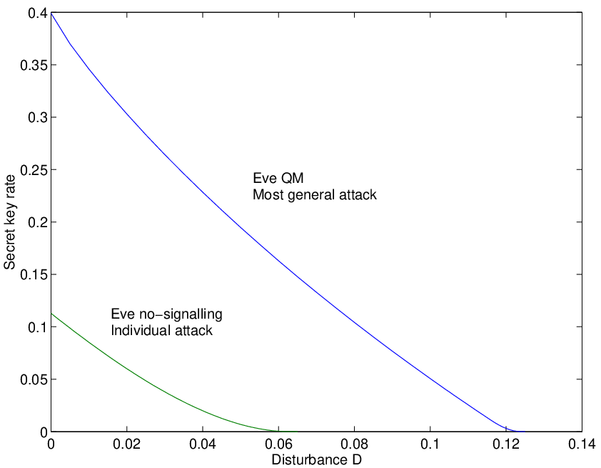
This quantity is plotted in Fig. 2 as a function of the disturbance defined by . This parameter characterizes the properties of the channel linking Alice and Bob: it is therefore useful for comparison with a quantum realization of the CHSH protocol and with BB84, see III.7 and Appendix A. We see that for that is for the optimal pre-processing. Without pre-processing, the bound becomes . The important remark is that both these values are within the quantum region (16). This means that using quantum physics, one can distribute correlations which allow (at least against individual attacks) the extraction of a secret key without any further assumption about the details of the physical realization.
III.5.3 Reaching the Bell limit
Another interesting example deals with the following question: can one find one-parameter families of probability distributions for which as soon as ; that is, distributions for which one can extract a secret key out of one-way processing, down to the limit of the local polytope? The answer is yes, and this can be achieved even without pre-processing. Here is an example: set , , and . For both and we have . For , Alice and Bob make no errors (), and Eve’s information is ; for , the errors of Alice and Bob are and Eve has no information. In summary, even neglecting pre-processing,
| (34) |
which is strictly positive in the whole region .
Note that the distributions described here cannot be broadcasted using quantum states. The reason is that the quantum intersection with the non-local region is strictly inside this region, where ”inside” means that, as soon as , all the must be non zero, because the are linearly independent. On the contrary, here we have set . Anyway, in spite of the fact that we are not able to broadcast this distribution with known physical means, it is interesting to notice that there exists a family of probability distributions that can lead to a secret key under one-way post-processing, for any amount of non-locality.
III.6 Two-way classical post-processing
III.6.1 Advantage distillation (AD)
Contrary to the one-way case, no tight bound like the Csiszár-Körner bound is known when two-way classical post-processing is allowed; nor is the optimal procedure known. The best-known two-way post-processing is the so-called advantage distillation (AD). Forgetting about pre-processing, one can see the effect of AD as follows: starting from a situation where , one makes a processing at the end of which the new variables satisfy ; at this point, one applies the one-way post-processing.
In AD, Alice reveals instances such that her bits are equal: . Bob looks at the same instances, and announces whether his bits are also all equal. If indeed , which happens with probability , Alice and Bob keep one instance; otherwise, they discard all the bits. Bob’s error on Alice’s symbols becomes
| (35) |
Notice that in the limit : this means that almost always, for sufficiently large. This remark is used to estimate Eve’s probability of error (see below for concrete applications). Typically, one finds that Eve’s error on Bob’s symbols goes as
| (36) |
with some function which depends on the probability distribution under study. Now, as long as the condition
| (37) |
is fulfilled, Eve’s error at the end of AD is exponentially larger than Bob’s for increasing : there exists always a finite value of such that Eve’s error becomes larger than Bob’s. The bound on the tolerable error after AD is then computed by solving eq. 37.
We apply this procedure to the isotropic correlations described above (III.5.2), first without pre-processing, then by allowing Alice and Bob to perform some bit flip before starting AD. We anticipate the result: we find that a key can be extracted for ; that is, even with two way post-processing we are not able to reach the Bell limit for isotropic correlations. It is an open question, whether the Bell limit can be reached by a better two-way post-processing for the isotropic distribution.
III.6.2 AD without pre-processing
We refer to Table 3. We have, as above, . We must now estimate Eve’s error on Bob’s symbol after AD. Eve knows as soon as she knows one of Alice’s symbols , and recall that asymptotically the guess is correct. The only situation in which Eve is obliged to make a random guess is therefore the case in which all the instances correspond to Eve’s symbol . The probability that Eve’s guess of Bob’s symbol is wrong is therefore
| (38) |
where the denominator comes from the fact that we must condition on the bit’s acceptance. Using (37), we obtain that secrecy can be extracted as long as that . This is lower than the bound obtained for one-way post-processing, as expected.
III.6.3 AD with pre-processing
The previous bound can be further improved by allowing Alice and Bob to pre-process their lists before starting AD. For two-way post-processing, it is not known whether bitwise pre-processing is already optimal; but we restrict to it in this work. Specifically, we suppose that Alice flips her bit with probability , Bob with probability . By inspection, one finds that the probability distribution obtained from Table 3 after this pre-processing is the one of Table 4, where we have written . Just by looking at the Table, one can guess the interest of pre-processing: the five possible symbols for Eve are now spread in all the four cells of the table. For instance, Eve’s symbol is was present only in the case in Table 3, that is, whenever she had this symbol Eve had full information; this is no longer the case in Table 4. Note also that the roles of and are not symmetric, because only mixes the strategies for which Eve does not know Bob’s symbol.
The distribution of Table 4 is such that
| (39) |
The estimate of Eve’s error requires some attention. As before, we assume that as soon as Eve guesses correctly Alice’s symbol , she automatically guesses also ; so the question is, when is Eve uncertain about , in the asymptotic regime of large ? Of course, inequality (38) still holds with replacing ; but this condition is too weak here: it does not make any use of the uncertainty introduced on Eve’s knowledge by the pre-processing.
Eve’s situation now is such that, even if she has a symbol or , she cannot be completely sure whether or not. Suppose that among her symbols, Eve has times the symbol , times the symbol , times the symbol , times the symbol , and times the symbol . Eve cannot avoid errors when , that is when and . We have therefore the bound
| (40) |
where the sum is taken under the constraint , is the probability that Eve has symbol conditioned on the bit’s acceptance, and , . By using and summing the multinomial expansion, we obtain
| (41) |
Now we must find the expressions for the in Table 4. Suppose for definiteness that Alice and Bob have accepted the bit : this happens with probability . The probability that this happens and that Eve has got the symbol is ; whence . Similarly, the probability that Alice and Bob accept the bit 0 and that Eve has got , respectively , is , respectively ; whence . In a similar way, one computes . By writing , we have then
and the condition for extraction of a secret key becomes
| (46) |
The optimization over and can be done numerically. The result is that a secret key can be extracted at least down to .
III.6.4 Positivity of intrinsic information
Given a tripartite probability distribution, , an upper bound to the secret-key rate is given by the so-called intrinsic information , denoted more briefly in what follows by . This function, introduced in [26], reads
| (47) |
the minimization running over all the channels . Here, denotes the mutual information between Alice and Bob conditioned on Eve. That is, for each value of Eve’s variable , the correlations between Alice and Bob are described by the conditioned probability distribution . The conditioned mutual information is equal to the mutual information of these probability distribution averaged over . The exact computation of the intrinsic information is in general difficult. However, a huge simplification was obtained in [27], where it was shown that the minimization in Eq. (47) can be restricted to variables of the same size as the original one, . This allows a numerical approach to this problem.
The intrinsic information can be understood as a witness of secret correlations in . Indeed, a probability distribution can be established by local operations and public communication if, and only if, its intrinsic information is zero [28]. It is then clear why the positivity of the intrinsic information is a necessary condition for positive secret-key rate. Whether it is sufficient is at present unknown: strong support has been given to the existence of probability distributions such that and . These would constitute examples of probability distributions containing bound information [29], that is non-distillable secret correlations. The existence of bound information has been proven in a multipartite scenario consisting of honest parties and the eavesdropper [30]. However, it remains as an open problem for the more standard bipartite scenario.
Using these tools, it is possible to study the secrecy properties of the probability distribution derived from the previous CHSH-protocol. A first computation of its conditioned mutual information gives . This result easily follows from Table 2: when , that happens with probability , Alice and Bob are perfectly correlated, so their mutual information is equal to one. In all the remaining cases, e.g. , Alice and Bob have no correlations. Using this observation, one can guess the optimal map . In order to minimize the conditioned mutual information, this map should deteriorate the perfect correlations between Alice and Bob when . A way of doing this is by mapping and into , leaving the other symbols unchanged [31]. We conjecture that this defines the optimal map for the computation of the intrinsic information. Actually, all our numerical evidence supports this conjecture. Thus, the conjectured value for the intrinsic information is
| (48) |
Interestingly, this quantity is positive whenever . If the conjecture is true, it implies that either (i) it is possible to have a positive secret-key rate for the whole region of Bell violation, using a new key-distillation protocol, or (ii) the probability distribution of Table 2 represents an example of bipartite bound information for sufficiently small values of .
III.7 Quantum cryptographic analysis of the CHSH protocol
It is interesting to analyze the CHSH protocol with the standard approach of quantum cryptography: Alice and Bob share a quantum state of two qubits and have agreed on the physical measurements corresponding to each value of and ; Eve is constrained to distribute quantum states, of which she keeps a purification. Recent advances have provided a systematic recipe to find a lower bound on the secret key rate, that is, to discuss security when Eve is allowed to perform the most general strategy compatible with quantum physics (such bounds have been called ”unconditional security proofs”, but it should be clear by all that precedes that this wording is unfortunate).
The resulting bound on the achievable secret key rate is plotted in Fig. 2. Since the formalism used to compute this bound is entirely different from the tools used in the present study, we give this calculation in Appendix A. It turns out that the CHSH protocol is equivalent to the BB84 protocol plus some classical pre-processing. In particular, the robustness to noise is the same for both protocols. For low error rate, BB84 provides higher secret-key rate; however, BB84 cannot be used for a device-independent proof, since (as we noticed above) its correlations become intrinsically insecure if the dimensionality of the Hilbert space is not known.
IV Larger-dimensional Outcomes
In this Section, we explore the generalization of the previous results to the case of binary inputs and -nary outputs: , ; that is, and . Below, all the sums involving dits are to be computed modulo .
For this study, it is useful to introduce a notation for probability distributions and inequalities [32]. While the full probability space is -dimensional, one can verify that only parameters are needed to characterize completely a no-signalling probability distribution — in other words, is the dimension of the space in which the no-signalling and the local polytopes are embedded. We choose the ( numbers for each value of ), the ( numbers for each value of ), and the ( numbers for each value of ). This we arrange in arrays as follows:
Note that this array has lines and as many columns: information on the values is redundant for all inputs because of no-signalling. Of course, there is no problem in working with the ”full” array with if one finds it more convenient, provided the additional entries are filled consistently because these parameters are not free.
This notation will also be used for inequalities: in this case, the numbers in the arrays are the coefficients which multiply each probability in the expression of the inequality. Examples will be provided below.
IV.1 Polytopes and the quantum region
IV.1.1 Known characterization
As one might expect, the characterization of the local and the no-signalling polytopes are an increasingly hard task, as the dimension of the output increases.
Numerical studies [17] have provided an unexpectedly simple structure for the local polytope for small : as it happened for , all the non-trivial facets appear to be equivalent to the Collins-Gisin-Linden-Massar-Popescu (CGLMP) inequality [33, 34, 17, 35]
It is conjectured that all non-trivial facets are equivalent to the CGLMP inequality for all . Anyway, our work is independent of the truth of this conjecture: we are going to study the possibility of secret key extraction for non-local distributions which lie above a CGLMP facet, irrespective of whether there exist inequivalent facets or not.
The no-signalling polytope appears to have a richer structure than in the case . All the extremal non-local points are generalizations of the PR-box [10]. We are interested in those that lie above our representative CGLMP facet. The highest violation of CGLMP is provided by the extremal point
| (63) |
whose corresponding array is
Its violation of the inequality can be rapidly calculated by a term-by-term multiplication (a formal scalar product) of the two arrays (IV.1.1) and (IV.1.1), yielding
| (74) |
However, is not the only non-local extremal point which lies above a CGLMP facet: in fact, for all , there is at least one above the facet. For instance, a possible version of reads (boldface standing for matrices filled with zeros)
whence a violation . For , we shall give below (IV.3) some additional elements on the structure of the no-signalling polytope.
The boundaries of the quantum region are basically unknown to date; it is not even clear whether they coincide with all possible results of measurements on two-qutrits states.
IV.1.2 A slice in the non-local region
As we said, a no-signalling probability distribution is characterized by parameters. However, when one reviews the results obtained for the CGLMP inequality in the context of quantum physics (see Appendix B for all details), one finds that the probability distributions associated to the optimal settings belong to a very symmetric family. Specifically, these distributions are such that (i) for fixed inputs and , depends only on ; and (ii) the probabilities for the different inputs are related as . Compactly:
| (95) |
with and . The corresponding array is
This family defines a slice in the no-signalling polytope. Note that all the marginals are equal, that is, . Moreover, the numbers define uniquely and completely a point in the slice; thus, given the constraint , the slice defined by (95) is -dimensional. A single extremal non-local point belongs to the slice, namely , obtained by setting (63); in fact, none of the with has the correct marginals.
As it happened for the isotropic distributions for , there exists a depolarization procedure that maps any probability distribution onto this slice by local operations and public communication, while keeping the violation constant. The procedure is given in Appendix C. As a consequence, Eve’s optimal individual eavesdropping, for a fixed value of the violation of the inequality, consists in distributing a point in the slice.
IV.2 Cryptography
IV.2.1 The protocol
We suppose from the beginning . The protocol is the analog of the CHSH protocol described in III.3 above. When Alice announces and Bob has measured , Bob corrects his dit according to . In other words, the pseudo-sifting implements . The Alice-Bob distribution after pseudo-sifting, averaged on Bob’s settings, becomes independent of (as in the case of isotropic distribution for ):
| (106) |
In a protocol with -dimensional outcomes, Alice and Bob can estimate not just one, but several error rates, one for each value of . We have just found that these error rates exhibit the symmetry
| (107) |
As in the case of bits, we think of Eve as sending either a local or a non-local probability distribution. Let’s discuss in some detail the points which lie on and above a CGLMP facet.
IV.2.2 Eve’s strategy: local points
To understand what follows, we don’t need a full characterization of the deterministic strategies that saturate the CGLMP inequality. Some facts are however worth noting; the proof of these statements and some other features are given in Appendix D.
The first fact is that, for , the number of deterministic points on the CGLMP facet is strictly larger than , the dimension of the local and the no-signalling polytope. This implies that, for some points on the facet, several decomposition as a convex combination of extremal points are possible.
The second fact is that no extremal deterministic strategy belongs to the slice (95): to see it, just recall that the marginals in the slice are completely random. Since we require the final distribution to belong to the slice, Eve must manage to send deterministic strategies with the suitable probabilities. As a consequence of the previous remark, at least one local point on the slice can be obtained by several different decompositions on extremal points: we’ll have to choose the decomposition that optimizes Eve’s information.
As a third fact, we elaborate on the same idea that lead to the uncertainty relations in paragraph III.4. We know that all deterministic strategies are not equally interesting for Eve, in fact, two kind of local points are of special interest for her: (i) those for which , because Eve knows Bob’s symbol when Alice announces , and which we denote by the set ; and (ii) those for which , because Eve knows Bob’s symbol when Alice announces , and which we denote by the set . In all the other cases, Eve does not learn Bob’s symbol with certainty. Now, in the complexity of the list of deterministic points on the CGLMP facet, a remarkable feature appears:
- •
There are exactly points in , namely those for which and can take any value. In other words, there are no points on the CGLMP facet such that but is different from this value: whenever Eve learns Bob’s symbol for , Alice and Bob make no error for .
- •
There are exactly points in , namely those for which and can take any value. This has a similar interpretation as the statement above, in the case .
Now, since the error rate Alice-Bob depends only on , and not on the particular decomposition chosen by Eve to realize this distribution, it is obvious that Eve’s interest lies in distributing local points that belong to as often as possible. For , we shall prove that she can prepare any point in the slice by distributing only these kind of local points. Finally, we want to introduce a further distinction within , which appears explicitly in the study of but may play a more general role. We shall call the subset of , whose points satisfy three out of the four relations , , and ; the complementary set, containing the points that satisfy two of the relations ( or ), is written .
IV.2.3 Eve’s strategy: non-local point
We have said that, among the extremal non-local points which lie above the CGLMP facet, the only one on the slice (95) is . However, it may be the case that mixtures of other extremal non-local points lie as well in the slice. For , this is not the case (see Appendix E), but we have not been able to generalize this statement. In this study, we suppose tentatively that Eve sends a unique non-local strategy, namely . Under this assumption, we can define as the probability that Eve sends . To find the expression of , we notice that should correspond to , and that for all local points on the CGLMP facet, should correspond to . Moreover, measures the geometrical distance from the facet and is therefore an affine function of the violation of CGLMP. Thus for a generic distribution of the form (IV.1.2) we have
| (108) | |||||
IV.3 Secret key extraction:
IV.3.1 The slice of the polytope
The slice (95) is 2-dimensional for , we choose and as free parameters; this gives and
| (109) |
The full slice has a form of an equilateral triangle (Fig. 3), whose vertices are defined by . As mentioned, . The vertex is also a , the one defined by with . On the contrary, a mixture of deterministic strategies. The middle of the triangle, , is the completely random strategy (obtained e.g. when measuring the maximally mixed quantum state, the ”identity”).

We are going to focus on the non-local region close to (Fig. 4). The intersection with the CGLMP facet is the segment , whose ends are the points labelled (, ) and (, ). The decompositions of these mixtures on the extremal deterministic strategies are
| (110) |
where the sets of local points and have been defined above. In fact, the decomposition of is unique; conversely, can be decomposed in an infinity of ways (see Appendix E), but all the others involve also the points that don’t belong to and are therefore sub-optimal for Eve.

The quantum-mechanical studies (see Appendix B for more details) have singled out two non-local probability distributions in this region. The first one corresponds to the maximal violation of CGLMP using two qutrits, : it is noted and is defined by (B) with . The second one corresponds to the highest violation achievable with the maximally entangled state of two qutrits, : it is noted and is defined by (B) with .
IV.3.2 One-way classical post-processing
To write down the table for the correlations Alice-Bob-Eve, one needs to list explicitly the deterministic points that saturate CGLMP and the corresponding information Eve can extract. This is done in Appendix E. The result is Table 5. It can be verified easily that all the probabilities in a row/column sum up to ; moreover,
| (111) |
as expected from (107). We have introduced the symbol to describe the situation where Eve is uncertain on Bob’s symbol, but only among two possibilities: this is clearly the case whenever the uncertainty derives from a deterministic strategy. In all that follows, information is quantified in trits, and we write .
In the absence of pre-processing, Eve has no information with probability , full information with probability , and information with probability . Therefore the estimate for the CK bound is
| (112) | |||||
The curve is shown in Fig. 4, it clearly cuts the quantum region.
A natural question is, which is the point that maximizes under the requirement that the correlations should belong to the quantum region. In the slice under consideration, we find a rate trits bits for the correlations defined by , . These correlations can be obtained by measuring the quantum state
| (113) |
for . This state is close to, but certainly different from, the maximally entangled state. Thus, the secret key rate exhibits the same form of anomaly as all the other measures of non-locality known to date [45]: maximal non-locality is obtained with non-maximally entangled states.
We consider now Bob’s pre-processing. For one-way post-processing, dit-wise pre-processing is already optimal. A priori, one can define two different flipping probabilities and , associated respectively to and . But it turns out by inspection that the optimal is always obtained for , so we write down directly this case. From (111) it is clear that after pre-processing
| (114) |
whence
| (115) |
Eve’s information is computed by recalling that, for any local point she sends out, before pre-processing (i) for one value of , she knows perfectly Bob’s symbol ; (ii) for the other value of , she hesitates between two values of . Pre-processing leaves unchanged with probability , and sends it to with probability each. Therefore, in case (i), Eve’s information is lowered from 1 to ; in case (ii), Eve’s information is lowered from to . Since each case is equiprobable,
| (116) |
From (115) and (116), we can compute by optimizing the value of . We did the optimization numerically. The improvement due to pre-processing is clear in Fig. 4.
IV.3.3 Two-way classical post-processing
We have also studied the possibility of extracting a secret key from the correlations of Table 5 using AD (without pre-processing). Alice selects of her symbols that are identical, Bob accepts if and only if his corresponding symbols are also identical. The probability that Bob accepts is , and consequently
| (117) |
As in the case , Eve has to make a random guess if and only if she has sent for all the instances:
| (118) |
Thus, a secret key can be extracted using AD as long as , that is as long as
| (119) |
The limiting curve is also plotted in Fig. 4. Its extremal points are for (the same value as obtained for ) and for .
IV.3.4 Intrinsic information
It is straightforward to generalize the map used above in the computation of the intrinsic information to the case. Looking at table 5, one has to map all the symbols into , where . The obtained conditional mutual information reads
| (120) | |||||
This is of course an upper bound to the intrinsic information, since the employed map may not be the optimal one. Contrary to what happens in the case, this quantity vanishes for some points inside the region of Bell violation! Indeed, Eq. (120) is zero on the line ; by changing slightly Eve’s map (specifically, she applies the map above only with a suitable probability and makes nothing in the other cases), it can be verified that the intrinsic information is zero also below the line, that is for
| (121) |
This region overlaps with the non-local region (Fig. 4).
IV.4 Secret key extraction: generic
For generic , we want to prove that secrecy can be generated using quantum states. The statistics Alice-Bob can be computed using quantum mechanics, in particular the error rates of Eq. (107). The question is, how to estimate Eve’s information: to compute this quantity exactly, one must describe the points in the CGLMP facet in some detail. However, some interesting bound can be derived from what we have already said and the intuition developed in the study of .
Consider first one-way post-processing: the discussion of paragraph IV.2.2 implies the bound
| (122) |
The bound is reached if and only if Eve distributes strategies that belong to , as it happened to be always possible for . Moreover, this bound can also be computed from the Alice-Bob distribution only assuming (108). Consequently we can estimate
| (123) |
with the Shannon entropy measured in dits. We have studied the r.h.s. numerically for , for correlations in the quantum region obtained from states that are Schmidt-diagonal in the computational basis, . The general features that emerge are:
- •
The maximal value of achievable in the quantum region increases with , reaching up to bits for .
- •
The quantum state corresponding to the maximal value of is always such that . It seems that the overlap of this state with the maximally entangled one decreases with , but the decrease is very slow (we have for , and for we still have ).
A similar simple approach can be found to explore the possibilities of two-way post-processing. We have
| (124) |
and Eve’s error is . Consequently, AD will certainly work for
| (125) |
All the quantities in this relation can be computed from the Alice-Bob correlations alone. As before, we have studied this condition numerically, for . This time, we have concentrated on correlations of the form , where are the correlations obtained when measuring the maximally entangled state (this is of course a completely arbitrary choice, but seems interesting from the point of view of quantum physics). One observes that, as expected, the use of two-way post-processing significantly decreases the value of for which no secrecy can be extracted. Moreover, decreases when increases, but very slowly; so slowly in fact, that it cannot be guessed from the numerical results whether ultimately for .
In summary, we have obtained a few results for generic . In spite of a large number of assumptions and approximations (not least the choice of the protocol), we can conjecture that secrecy can be extracted from quantum non-local correlations for any ; and more precisely, that the amount of extractable secrecy increases with increasing .
V Conclusions and Perspectives
In conclusion, we have presented a first approach to a device-independent security proof for cryptography, expanding and generalizing the work of Ref. [4]. Under the assumption of individual attacks, we have proved that a secret key can be extracted from some no-signalling probability distributions, using only the very fact that they violate a Bell-type inequality and cannot therefore originate from shared randomness. In particular, noisy quantum states can be used to distribute correlations, that are non-local enough to contain distillable secrecy: so our result is also of practical interest.
We’d like to finish by raising some of the questions and perspectives that are opened by this work.
- •
A first objective is to extend our analysis beyond the assumption of individual attacks, proving ultimately the security against the most general attacks by an eavesdropper limited by no-signalling. A first step in this direction has been recently derived [36].
- •
One can make a step further: can one make a device-independent proof of security against an eavesdropper which would be limited by quantum physics? On the side of Alice and Bob, non-locality should still be the physical basis for security, because there exist no other entanglement witness which works independently of the dimension of the Hilbert space. On the side of Eve, the requirement that she must respect quantum physics is a limitation, compared to power we gave her in this paper; so one can hope to obtain a device-independent proof with better bounds.
- •
In this paper, we have defined protocols which look as ”natural” for the CHSH and the CGLMP inequalities. But there is no claim of optimality. In fact, it is not even proved that the pseudo-sifting that we have used is the best way of extracting secrecy from the raw correlations of CHSH-like measurements (Table 1). Other protocols may be better suited for cryptographic tasks, as discussed in Ref. [37].
- •
A particular consequence of the previous item is worth mentioning in itself. On the one hand, it has been proved that all non-local probability distributions have positive intrinsic information [25]. On the other hand, as mentioned several times in this paper, we have not been able to find an explicit procedure for extracting a secret key in the whole non-local region. This means, either that a better procedure does exist, or that non-local distributions close to the local limit provide examples of bipartite bound information [29, 30].
- •
A technical open point, which we mentioned and would be very meaningful for the present studies, is the characterization of the quantum region in probability space for a given number of inputs and outcomes.
Acknowledgements
We thank Stefano Pironio, Sandu Popescu and Renato Renner for discussion. This work has been supported by the European Commission, under the Integrated Project Qubit Applications (QAP) funded by the IST directorate as Contract Number 015848, and the Spanish MEC, under a Ramón y Cajal grant. We acknowledge also financial support from the Swiss NCCR ”Quantum Photonics”.
Appendix A Lower bound for a quantum implementation of the CHSH protocol
In this appendix, we study the security of the CHSH protocol in the standard scenario where Eve is limited by the quantum formalism, and Alice and Bob have a perfect knowledge on their quantum devices. More precisely, Alice and Bob know their Hilbert spaces are two-dimensional and they apply the spin measurements that produce the largest Bell violation for the noiseless state . For instance, Alice and Bob measure in the plane, their spin measurement being defined by the angle with the axis on the Poincaré sphere. Alice measures in the and bases, corresponding to respectively, while Bob does it in the directions, corresponding to .
As shown in Refs [38, 39], the bound for security against the most general attacks (”unconditional security”) can be computed by focusing on ”collective attacks”, where Eve prepares the same two-qubit state on all instances, but is allowed to make a coherent measurement of her ancillae after error correction and privacy amplification.
By inspection, or by using the formalism developed in Ref. [38], it can be proved that Eve’s optimal strategy uses a Bell-diagonal state of the form
| (126) |
where and denote the projectors onto the Bell basis
| (127) |
By assumption, Eve holds a purification of each pair: before any measurement, the quantum correlations among Alice, Bob and Eve are described by the pure state where .
In the CHSH protocol, Alice and Bob’s bases do not perfectly overlap: their outcomes are therefore not perfectly correlated even in the case (perfect channel, no Eve): actually, the quantum bit error rate (QBER) in this case is . For the same channel, the BB84 protocol has zero QBER. In the light of this, the meaningful parameter to compare the two protocols should not be the QBER, but a measure of the quality of the channel. We use the disturbance, that is the probability that measurement outcomes in the same basis agree: in our case, .
Now, Alice and Bob measure their local systems, while Eve keeps her quantum state. In this scenario, a lower bound to the key rate distillable using one-way communication protocols has been obtained in [40],
| (128) |
Here, denotes the standard mutual information between Alice and Bob’s classical outcomes, while is the Holevo quantity for the effective channel between Bob and Eve. Indeed, Bob’s measurement outcome prepares a quantum state on Eve’s site (see [40] for more details). Contrary to the more standard situation, Eve does not know which measurement Bob has applied, so she has to sum over the two possibilities. Her states read, up to normalization,
| (129) |
where and denote the basis elements in the direction specified by , as above. It is straightforward to see that for the CHSH protocol
| (130) |
The computation of , where denotes the von Neumann entropy for a state , is slightly more involved. However, after some patient algebra one can see that the maximum of this quantity is obtained, for fixed disturbance, when
| (131) |
which defines Eve’s optimal attack. Not surprisingly, this attack corresponds to a phase covariant cloning machine (see for instance [41]), that optimally clones all the states in the plane. This attack is also optimal for the standard BB84 protocol.
The obtained critical disturbance for CHSH is . This is larger than the well-known Shor-Preskill bound for security of BB84 [42]. This bound, however, has recently been improved by allowing any of the parties, say Alice, to introduce some pre-processing of her outcome before the reconciliation [38]. Alice then flips her bit with probability . This local noise worsens the correlations between Alice and Bob but it deteriorates in a stronger way the correlations between Alice and Eve. For any value of the disturbance there exists an optimal pre-processing , depending on the protocol, which maximizes the key rate. This explains the improvement on the critical disturbance that moves up to both for BB84 and for the CHSH protocol described here.
Actually, the close relation between the CHSH protocol and the BB84 protocol is made clear by this pre-processing. Let and be respectively the QBER and the pre-processing rate for BB84; and and denote the same quantities for the CHSH protocol. Note first that the channel defined in (131) induces a QBER in BB84, and a QBER for the CHSH protocol; whence
| (132) |
It can then be shown that when the QBERs are related as (132) and when
| (133) |
These two relations imply
| (134) | |||||
Consider first for clarity the case : the error in CHSH due to the non-perfect overlap of the bases can be attributed to the application of a pre-processing onto the correlations obtained with perfectly overlapping bases (indeed, the errors are intrinsic to the protocol, and Eve cannot gain anything from them). In general, the rates obtained for the CHSH protocol in the standard quantum scenario coincide with those derived for the BB84 protocol when the pre-processing is optimized under the constraint . If we now compare and for a fixed value of [that is, (132) holds] and choosing the optimal pre-processing in each case, we find the following. For small error rates, the optimal pre-processing on BB84 is smaller than ; in other words, even for CHSH corresponds to BB84 with an excessive pre-processing, whence . The optimal pre-processing on BB84 becomes equal to for ; from this point on, the optimal is larger than zero, and the rates for the two protocols become identical: . In particular, as announced, both become zero for .
Appendix B The CGLMP inequality in quantum physics
The CGLMP inequalities [33] have been the object of several studies in the context of quantum physics. Here we summarize the results without any proof.
One unexpected features of CGLMP is the fact that the maximal violation is not reached by measurements on the maximally entangled state [43]. Also unexpected is the fact that the settings that maximize the violation are the same for a wide class of states (including the maximal entangled one and the one which gives the maximal violation). These are the settings we consider here. We label them and for Alice, and for Bob:
| (135) | |||||
| (136) |
In operational terms, both Alice and Bob apply first global phases in the computational basis, then make a quantum Fourier transform (Bob makes the inverse as Alice), and finally measure in the new basis and outcome the value or .
Consider quantum states that are Schmidt-diagonal in the computational basis:
| (137) |
with : on this family, one finds
| (138) | |||||
with . The only freedom left is the choice of the four angles and . The settings we are interested in are defined by
| (139) |
With these settings, (95) holds.
For the case , all the interesting states found to date are of the form (113). For instance, is the maximally entangled state; the maximal violation is obtained for [43]; the largest Kullback-Leibler distance from the set of local distributions is obtained for [44]; and we have shown above (IV.3) that the maximal amount of secret key rate under one-way processing is found for . For the states , the are:
Appendix C Depolarization for arbitrary
C.1 The procedure
Suppose Alice and Bob share initially an arbitrary no-signalling probability distribution . The depolarization procedure that brings in the slice defined by (95) is very similar to the one described in Ref. [25] for . It consists of two steps.
Step 1. Alice chooses with probability and communicates it to Bob on a public channel. Both Alice and Bob perform
This implements which is such that and is consequently a function only of .
Step 2. With probability , Alice chooses one of the following four procedures and asks Bob on the public channel to act accordingly:
where we have written . This implements such that
Because of the symmetry of , this implies which is nothing but the definition of the slice (95).
C.2 Examples
We said in the main text that none of the extremal points of the form , with , is on the slice. Let’s then consider a realization of , the one whose array is
where boldface numbers indicate arrays containing all ones or all zeros, is the identity matrix of dimension , and where is the matrix
The arrays (IV.1.1) and (C.2) allow to compute immediately the ”scalar product”
| (173) |
generalizing the results we gave in the main text for and .
By following the steps of the depolarization protocol, one finds that goes to the distribution in the slice which is given by
and obviously all the other are zero. Using (108), one can verify that : the violation is preserved. As we said in the main text, this is not peculiar to this example, but is a general feature, as we show in the next paragraph.
C.3 Preservation of the violation of CGLMP
We want to prove that this depolarization preserves the violation of the CGLMP inequality, that is
| (177) |
The easiest way is to write down as it appeared in the original paper [33], namely with
where . The link between and our definition of is provided by
| (178) |
Using the expression of , the proof is straightforward. In fact, Step 1 keeps by definition all the constant, while Step 2 keeps both sums in constant.
Appendix D Deterministic strategies that saturate CGLMP
We present here a more detailed study of the extremal points that lie on the CGLMP facet, completing what has been written in paragraph IV.2.2.
Consider the array which represents the CGLMP inequality , eq. (IV.1.1); here, it is more convenient to look at it as having entries [35]. Let denote an entry of this array. For the deterministic strategy , the value of CGLMP is simply
| (179) | |||||
where the comes from the marginals of and , and where is equal to 1 if condition is satisfied and to 0 otherwise. The inequality is saturated by all the strategies such that .
Consider the points such that : the last two conditions become equal and the ’s compensate each other for all , so the only way to saturate the inequality is to fulfill both and ; whence as announced in the main text. The proof of the analog statement in the case is similarly done by inspection. One first considers : in this case, , therefore the first two conditions cannot be both fulfilled, whatever is. One can then easily verify that only the choice leads to a saturation of the inequality. The last remaining case is , : it can be read directly from the array, and leads to the same conclusion.
So, we have proved the properties of sets and , which consist of points each; we still have to prove that the number of points on the facet is larger than . This is easily done by noticing the following: the four ”natural” relations associated to the CGLMP inequality, those that are simultaneously fulfilled by , are:
Because of the specific pseudo-sifting of our cryptographic protocol, we grouped them by pairs according to Alice’s input. But from the standpoint of the inequality, any pairwise grouping is equally meaningful. It can indeed be easily verified using (179) that all the points that fulfill at least two among these relations saturate the inequality. There are therefore strategies that fulfill three relations, and strategies that fulfill exactly two relations. In conclusion, by looking only at the points that fulfill at least two among the four relations (D), we have already deterministic points on the CGLMP facet, and this number is larger than for . We note that the list is exhaustive for (see Appendix E), but not in general. For instance, for , the strategy fulfills none of the relations (D), but achieves nevertheless .
Appendix E Explicit analysis for
E.1 Deterministic strategies on the facet
We give here the explicit list of the 30 deterministic strategies that saturate CGLMP. We note .
The twelve strategies in are
The six strategies in are
| (191) | |||||
| (192) |
The twelve strategies outside are:
As we said in the main text, the decomposition of given in (110) is only one possible decomposition, the one which optimizes Eve’s information on Bob’s symbol. It can checked that the general decomposition is defined by
There are thus six free parameters , constrained of course by the positivity of probabilities (in particular, none of these parameters can exceed ). A possible realization of is the equiprobable mixture of the eighteen points which are not in . The choice leading to (110) is the equiprobable mixture of the six points in (, implying automatically ).
E.2 Alice-Bob-Eve correlations
Having the explicit deterministic strategies, it is a matter of patience to derive the Tables for the correlations Alice-Bob-Eve. The result is given in Table 6, in which we have introduced the notations
| (205) |
Note that, in each of the nine cells, the sum of the probabilities does not depend on the , as it should: the decomposition of is known only to Eve. Eve is obviously interested in maximizing the probability of knowing both symbols, measured by ; whence the choice made in the main text.
E.3 About non-local points that violate CGLMP
Here, we want to list some non-local points other than , that violate CGLMP, and study their relation with the slice (95).
Consider first the non-local points equivalent to . There are 24 such points in the no-signalling polytope: in fact, there a three choices for the two outcomes [(0,1), (0,2) or (1,2)] and for each choice there are eight PR-like points, obtained as usual by relabelling inputs and/or outputs. By inspection, it can be seen that (in fact, ) for our representative (IV.1.1) of , is achieved only by three PR-like points: those defined by
| for |
It is readily seen that no mixture of these three strategies can belong to the slice (95): to obtain all the marginals equal to , the only possible mixture is the equiprobable one. This one reads
and is clearly not of the form (IV.1.2). This negative result is important for our study: had such a mixture belonged to the slice, Eve would have sent these non-local points, for which she would have gained some information (because in each case one result is impossible).
Actually, there is a mixture of non-local points on the slice: it is a mixture of other -like strategies, which optimize the violation of different representatives of CGLMP, and violate our representative by . The strategies are those in which is equal to , , and (note that this last one is indeed a : the non-locality is embedded on the fact that the r.h.s. is computed modulo 2, instead of modulo 3 as is the case for the others). The equiprobable mixture of these four strategies is the point and in the slice. Obviously, Eve has no interest in sending these strategies instead of the which gives the maximal violation: in all cases, she is going to learn nothing about the outcomes.
TABLES
| [isotropic] | ||
|---|---|---|
| x | |||
|---|---|---|---|
References
- [1] N. Gisin, G. Ribordy, W. Tittel, H. Zbinden, Rev. Mod. Phys 74, 145 (2002)
- [2] M. Dušek, N. Lütkenhaus, M. Hendrych, quant-ph/0601207; to appear in: Progress in Optics, vol. 49, Edt. E. Wolf (Elsevier)
- [3] J. Barrett, L. Hardy, A. Kent, Phys. Rev. Lett. 95, 010503 (2005)
- [4] A. Acín, N. Gisin, L. Masanes, quant-ph/0510094
- [5] We stress explicitly an important point. There are several ways of guaranteeing that no information leakage has taken place about and . One of these ways is based on physics: if the measurement-and-detection events of Alice and Bob are space-like separated events, then relativity guarantees that no signal has propagated from one location to the other. This is a sufficient, but not a necessary condition for independence. Our work only assumes that indeed there is no information leakage, independently of the way this is achieved.
- [6] A. Ekert, Phys. Rev. Lett. 67, 661 (1991)
- [7] The idea, that quantum correlations are ultimately the unique way of guaranteeing the ”quantumness” of an apparatus, appears in: D. Mayers, A. Yao, Quant. Inf. Comput 4, 273 (2004); F. Magniez, D. Mayers, M. Mosca, H. Ollivier, quant-ph/0512111.
- [8] B.S. Tsirelson, Hadronic J. Supplement 8, 329 (1993)
- [9] I. Pitowski, Quantum Probability, Quantum Logic, Lecture Notes in Physics 321 (Springer Verlag, Heidelberg, 1989)
- [10] J. Barrett, N. Linden, S. Massar, S. Pironio, S. Popescu, D. Roberts, Phys. Rev. A 71, 022101 (2005)
- [11] R.F. Werner, M.M. Wolf, Phys. Rev. A 64, 032112 (2001), paragraph V.C, and references therein.
- [12] C. H. Bennett, G. Brassard, in Proceedings IEEE Int. Conf. on Computers, Systems and Signal Processing, Bangalore, India (IEEE, New York, 1984), pp. 175-179.
- [13] See e.g. P.W. Shor, J. Preskill, Phys. Rev. Lett. 85, 441 (2000)
- [14] M. Curty, M. Lewenstein, N. Lütkenhaus, Phys. Rev. Lett. 92, 217903 (2004)
- [15] A. Acín, N. Gisin, Phys. Rev. Lett. 94, 020501 (2005)
- [16] A. Fine, Phys. Rev. Lett. 48, 291 (1982)
- [17] D. Collins, N. Gisin, J. Phys. A: Math. Gen. 37 1775 (2004)
- [18] J.F. Clauser, M.A. Horne, A. Shimony, R.A. Holt, Phys. Rev. Lett. 23, 880 (1969)
- [19] If the polytope is embedded in a -dimensional space, a facet is a hyperplane of dimension . To define such a hyperplane, one needs linearly independent points — just as one needs two different points to define a line, three non-aligned points to define a plan etc.
- [20] S. Popescu, D. Rohrlich, Found. Phys. 24, 379 (1994)
- [21] B.S. Cirel’son, Lett. Math. Phys. 4, 83 (1980)
- [22] H.-K. Lo, H.F. Chau, M. Ardehali, J. Cryptology 18, 133 (2005); D. Stucki, N. Brunner, N. Gisin, V. Scarani, H. Zbinden, Appl. Phys. Lett. 87, 194108 (2005)
- [23] I. Csiszár, J. Körner, IEEE Trans. Inf. Theory 24, 339 (1978)
- [24] R. Ahlswede, I. Csiszár, IEEE Trans. Inf. Theory 39, 1121 (1993)
- [25] L. Masanes, A. Acín, N. Gisin, Phys. Rev. A 73, 012112 (2006)
- [26] U. Maurer and S. Wolf, IEEE Trans. Inf. Theory 45, 499 (1999).
- [27] M. Christandl, R. Renner and S. Wolf, Proc. ISIT 2003, 258, Yokohama, Japan.
- [28] R. Renner and S. Wolf, Adv. in Crypt., EUROCRYPT ’03, Lecture Notes in Computer Science, Springer-Verlag, 2003.
- [29] N. Gisin and S. Wolf, Proceedings of CRYPTO 2000, Lecture Notes in Computer Science 1880, 482, Springer-Verlag, 2000, quant-ph/0005042.
- [30] A. Acín, J. I. Cirac and L. Masanes, Phys. Rev. Lett. 92, 107903 (2004); L. Masanes and A. Acín, cs.CR/0501008, accepted for publication in IEEE Trans. Inf. Theory.
- [31] This map looks conter-intuitive from Eve’s point of view. Why should she map and , where she knows Alice’s variable, into ? Recall however that this map is only a mathematical tool for the computation of an upper bound on the secret-key rate.
- [32] We could have used the same formalism for the case ; we did not, because we found it preferable to tackle that case without the introduction of a lot of notations. Anyway, all that we write in Section IV for general applies in particular for .
- [33] D. Collins, N. Gisin, N. Linden, S. Massar, S. Popescu, Phys. Rev. Lett. 88, 040404 (2002)
- [34] L. Masanes, Quant. Inf. Comput. 3, 345 (2002)
- [35] The array (IV.1.1) that defines has exactly the same form, whether one considers it as having entries, or in the ”full” form which has entries. It is in fact easy to verify that the all the terms that are added cancel out.
- [36] L. Masanes, A. Winter, quant-ph/0606049
- [37] A. Acín, S. Massar, S. Pironio, quant-ph/0605246
- [38] B. Kraus, N. Gisin and R. Renner, Phys. Rev. Lett. 95, 080501 (2005).
- [39] R. Renner, Security of Quantum Key Distribution, PhD thesis, quant-ph/0512258.
- [40] I. Devetak and A. Winter, Proc. R. Soc. Lond. A 461, 207 (2005).
- [41] N. J. Cerf, Phys. Rev. Lett. 84, 4497 (2000)
- [42] P. W. Shor and J. Preskill, Phys. Rev. Lett. 85, 441 (2000).
- [43] A. Acín, T. Durt, N. Gisin, J.I. Latorre, Phys. Rev. A 65, 052325 (2002)
- [44] A. Acín, R. Gill, N. Gisin, Phys. Rev. Lett. 95, 210402 (2005)
- [45] For a review of the evidences of this anomaly, see: A.A. Méthot, V. Scarani, quant-ph/0601210.