Quantum Capacities of Bosonic Channels

Before we derive the main results we will briefly recall the basic notions HolevoBook; JWGauss. Consider a bosonic system of $N$ modes characterized by $N$ pairs of canonical operators $(Q_{1},P_{1},\ldots,Q_{N},P_{N})=:R$ for which the commutation relations $[R_{k},R_{l}]=i\sigma_{kl}$ are governed by the symplectic matrix $\sigma$. The exponentials $W_{\xi}:=e^{i\xi R},\;\xi\in\mathbb{R}^{2N}$ are called Weyl displacement operators. Their expectation value, the characteristic function, $\chi(\xi):={\rm tr}\left[{\rho W_{\xi}}\right]$ is the Fourier transform of the Wigner function and for Gaussian states it is a Gaussian

with first moments $d_{k}={\rm tr}\left[{\rho R_{k}}\right]$ and covariance matrix (CM) $\Gamma_{kl}:={\rm tr}\left[{\rho\{R_{k}-d_{k},R_{l}-d_{l}\}_{+}}\right]$. Note that coherent, squeezed and thermal states in quantum optics are all Gaussian states.

Gaussian channels JWGauss; Lindblad transform Weyl operators as $W_{\xi}\mapsto W_{X\xi}e^{-\frac{1}{4}\xi Y\xi}$ and act on covariance matrices as

Particularly important instances of single-mode Gaussian channels are attenuation and amplification channels for which $X=\sqrt{\eta}\mathbbm{1}$ and $Y=|\eta-1|\mathbbm{1}$. For $0\leq\eta\leq 1$ this models a single mode of an optical fiber with transmissivity $\eta$ where the environment is assumed to be in the vacuum state. The latter reflects the fact that thermal photons with optical frequencies are negligible at room temperature. For $\eta>1$ the channel becomes an amplification channel, where the noise term $Y$ is now a consequence of the Heisenberg uncertainty.

Teleportation channels: We will now derive the form of Gaussian channels which are obtained when teleporting through a centered bipartite Gaussian state. As this is useful for applying but not necessary for understanding the following it might be skipped by the reader. Let $\Gamma={\footnotesize\left(\begin{array}[]{cc}\Gamma_{A}&\Gamma_{C}\\ \Gamma_{C}^{T}&\Gamma_{B}\\ \end{array}\right)}$ be the CM of a Gaussian state of $N_{A}+N_{B}$ modes with $N_{A}=N_{B}$. Assume Bob wants to teleport a quantum state of $N_{B}$ modes with CM $\gamma$ to Alice. Using the standard protocol teleV he sends pairs of modes from $\gamma$ and $\Gamma_{B}$ through 50:50 beam-splitters, measures the $Q$ and $P$ quadratures, and then communicates the outcomes. Depending on the latter Alice applies displacements to the modes in $\Gamma_{A}$. The simplest way of deriving an expression for the output is to start with the Wigner representation and to assume that the state to be teleported is a centered Gaussian. The Wigner function before the measurement is up to normalization given by $\exp{-\xi\big[M_{BS}^{T}(\Gamma\oplus\gamma)^{-1}M_{BS}\big]\xi}$, where $M_{BS}$ corresponds to the beam-splitter operation. With $\xi=(\xi_{A},\xi_{B},\xi_{B^{\prime}})$ the final Wigner function is then proportional to

where $M_{X}$ incorporates the displacements, i.e., it is the identity matrix plus an arbitrary $2N_{B}\times 2N_{B}$ off-diagonal block which maps the $2N_{B}$ measurement outcomes onto the respective displacements. In order to circumvent integrating Eq.(3) we can now go to the characteristic function, i.e., the Fourier transformed picture. The integration then boils down to picking out the upper left block of the inverted matrix $\big[M_{X}^{T}M_{BS}^{T}(\Gamma\oplus\gamma)^{-1}M_{BS}M_{X}\big]^{-1}$. The inversion is, however, trivial since $M_{BS}^{-1}=M_{BS}^{T}$ and $M_{X}^{-1}$ is obtained from $M_{X}$ by changing the sign of all off-diagonal entries. In this way we obtain that the input CM is transformed to

where $\Lambda=\text{diag}(1,-1,1,-1,\ldots)$ and $X$ is such that $\sqrt{2}X$ is the matrix of displacement transformations, i.e., the gain which is typically chosen to be $\sqrt{2}\mathbbm{1}$.

Clearly, Eq.(4) has the form (2) and following the above lines it is straight forward to show that the channel is Gaussian and maps any (not necessarily centered Gaussian) input characteristic function $\chi_{in}$ into

For standard protocols ($X=\mathbbm{1}$) on single modes ($N_{A}=N_{B}=1$) this was derived in Scutaru.

The subject of interest is the quantum capacity $Q(T)$ of an arbitrary—a priori unknown—channel $T$. We will show how one can certify achievable rates for the transmission of quantum information through $T$ by only looking at the CM $\Gamma$ of a state $\rho_{T}=(T\otimes{\rm id})(\psi)$ which is obtained by sending half of an arbitrary entangled state $\psi$ through the channel. $\Gamma$ could be determined by homodyne measurements. The argument combines (i) the relation between entanglement distillation and quantum capacities observed in Bennett, (ii) the extremality of Gaussian states shown in CLT and (iii) the explicit form of Gaussian teleportation channels derived in the previous section. All together this leads to the chain of inequalities

Here $D_{\leftarrow}(\rho_{T})$ is the distillable entanglement under protocols with one-way communication (from Bob to Alice). Since a classical side channel does not increase $Q(T)$ this is clearly a lower bound to the capacity as Alice and Bob could simply first distill $\rho_{T}$ and then use the obtained maximally entangled states for teleportation Bennett. The second inequality uses that replacing $\rho_{T}$ by a Gaussian state ${\cal G}(\rho_{T})$ with the same CM $\Gamma$ can only decrease the distillable entanglement CLT. Finally, if we use the Gaussian state in turn as a resource for establishing a teleportation channel $T_{G}$ we end up with the sought inequality $Q(T)\geq Q(T_{G})$. $T_{G}$ is then the Gaussian channel in Eqs.(4,5), which is for a fixed teleportation protocol (a fixed matrix $X$) completely determined by $\Gamma$.

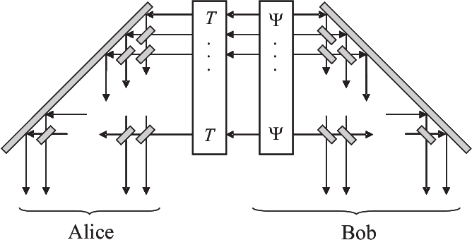
Bounds on the quantum capacity of Gaussian channels were derived in HolWer; GioShor and we will show below that it can be calculated exactly for some important cases. Note that a simple bound for $Q(T)$ can be obtained from a lower bound to $D_{\leftarrow}({\cal G}(\rho_{T}))$, the conditional entropy of the Gaussian state with CM $\Gamma$, i.e., $Q(T)\geq S(\Gamma_{A})-S(\Gamma)$.

Before we proceed, two comments on the quality of the above bound and its operational meaning are in order: The given argument holds for arbitrary $T$ and $\psi$. However, since we bound by Gaussian quantities the inequality might become trivial (i.e., $Q(T_{G})=0$ though $Q(T)\gg 0$) if both $T$ and $\psi$ are too far from being Gaussian. On the other hand, if $T$ is Gaussian and $|\psi\rangle=(\cosh r)^{-1}\sum_{n}(\tanh r)^{n}|nn\rangle$ is a two-mode squeezed state, then in the limit $r\rightarrow\infty$ the inequality becomes tight, i.e., $Q(T_{G})\rightarrow Q(T)$ with exponentially vanishing gap.

The first and last step in Eq.(6) have a simple operational meaning: sender and receiver first establish some entanglement, distill it and then use it as a resource for teleportation. The second step can also be understood in operational terms. To achieve $\rho_{T}\mapsto{\cal G}(\rho_{T})$ both sender and receiver have to apply an array of beam-splitters (see Fig.1) to many copies of the shared state $\rho_{T}$. Asymptotically every reduced state at the output will then converge to ${\cal G}(\rho_{T})$ CLT. By applying this gaussification to many different subsets, sender and receiver can then distill from or teleport through independent copies of ${\cal G}(\rho_{T})$ and in this way asymptotically simulate the channel $T_{G}$ via $T$.

It was proven in Qcap that the quantum capacity of a quantum channel $T$ can be expressed as

where $\psi$ is a purification of $\rho$ and $J$ is known as the coherent information. In general, the calculation of $Q(T)$ from the above formula is a daunting task since (i) the coherent information is known to be not additive, i.e., the regularization $n\rightarrow\infty$ is necessary, and (ii) due to lacking concavity properties there are local maxima which are not global ones. On top of this, for bosonic channels the optimization is over an an infinite dimensional space.

Fortunately, for a class of Gaussian channels including the important case of the lossy channel, these obstacles can be circumvented by exploiting recent results on degradability of channels DS; Gio2 and extremality of Gaussian states CLT.

To this end consider a channel $T(\rho_{S})={\rm tr}_{E}[U(\rho_{S}\otimes\varphi_{E})U^{\dagger}]$ expressed in terms of a unitary coupling between the system $S$ and the environment $E$ which is initially in a pure state $\varphi_{E}$. The conjugate channel $T_{c}(\rho_{S})={\rm tr}_{S}[U(\rho_{S}\otimes\varphi_{E})U^{\dagger}]$ is defined as a mapping from the system to the environment. As shown in DS the coherent information can be expressed in terms of a conditional entropy if there exists a channel $T^{\prime}$ such that $T^{\prime}\circ T=T_{c}$ — in this case $T$ is called degradable. More precisely, if $\tilde{\rho}_{S^{\prime}E^{\prime}}$ is the extension of the state $\tilde{\rho}_{S^{\prime}}=T^{\prime}\circ T(\rho)$ to the environment $E^{\prime}$ of $T^{\prime}$, then

The conditional entropy $S(E^{\prime}|S^{\prime})$ is known to be strongly sub-additive NC, i.e., for a composite system $S(E_{12}^{\prime}|S_{12}^{\prime})\leq S(E_{1}^{\prime}|S_{1}^{\prime})+S(E_{2}^{\prime}|S_{2}^{\prime})$. This has important consequences: for a set $\{T_{i}\}$ of degradable channels $J(\rho,\otimes_{i}T_{i})\leq\sum_{i}J(\rho_{i},T_{i})$, where $\rho_{i}$ are the corresponding reduced states, and if each $T_{i}$ is a Gaussian channel, we have in addition

The last inequality follows from the extremality of Gaussian states w.r.t. the conditional entropy JWGauss; CLT together with the fact that for Gaussian channels $T_{c}$ can be chosen to be Gaussian and the CM is transformed irrespective of whether the input was Gaussian or not.

As a consequence, if $T_{i}$ are degradable Gaussian channels, then

where the supremum is now taken only over Gaussian input states $\rho_{G}$. Calculating the latter for Gaussian channels is now a feasible task which was solved for the single-mode case in HolWer and in GioShor for broadband channels under power constraints using Lagrange multipliers. In fact, if we impose a constraint on the input energy of the form $\sum_{i}\omega_{i}N_{i}={\cal E}$, where $N_{i}$ is the average input photon number of mode $i$ with corresponding frequency $\omega_{i}$, then the above argumentation still holds, since the constraint just depends on the CM. The importance of Eq.(11) stems from the fact that a large class of Gaussian channels is indeed degradable, as shown in Gio2 and extended below. In particular we can apply Eq.(11) to attenuation (amplification) channels with transmissivity $\eta$ (gain $\sqrt{\eta}$). Together with the optimization carried out in HolWer this yields $Q$ as a function of $\eta$ (see Fig.2):

Note that the quantum capacity of every degradable Gaussian channel can easily be calculated as $J$ becomes a concave function of the CM such that local maxima are global ones. This is again a direct consequence of Eq.(9) together with the concavity of the conditional entropy NC and the extremality of Gaussian states JWGauss; CLT.

We will now investigate the condition under which Eq.(11) was derived and characterize the set of degradable Gaussian channels—extending the results of Gio2. To this end we represent the channel in terms of a unitary coupling between the system with $N_{S}$ modes and a (minimally represented) environment of $N_{E}\leq 2N_{S}$ modes which are initially in the vacuum state with $CM$ $\gamma_{E}=\mathbbm{1}$. The interaction is described by a symplectic matrix of size $2(N_{E}+N_{S})\times 2(N_{E}+N_{S})$ which we write in block form as $S={\footnotesize\left(\begin{array}[]{cc}A&B\\ C&D\\ \end{array}\right)}$ sympcond. The output CM of the channel $T:\gamma\mapsto X\gamma X^{T}+Y$ is then simply the lower right block of $S(\gamma_{E}\oplus\gamma)S^{T}$ (i.e., $D=X$ and $C\gamma_{E}C^{T}=Y$) whereas the conjugate channel $T_{c}$ corresponds to the upper left block.

Let us first focus on the case $N_{S}=N_{E}$ and assume for simplicity that the blocks in $S$ are non-singular. A channel is degradable if $T_{c}\circ T^{-1}$ is completely positive which is for a Gaussian trace preserving map equivalent to the condition Lindblad

Inserting the above block structure and using sympcond shows that complete positivity of $T_{c}\circ T^{-1}$ is equivalent to

Expressing this in terms of $X$ and $Y$ finally gives smallsteps

Similarly we can derive a condition for degradability of $T_{c}$ (anti-degradability of $T$) which is again given by the expressions (14, 15) which have then to be negative instead of positive semi-definite.

Since for $N_{E}=N_{S}=1$ $X$ is a $2\times 2$ matrix and thus $X\sigma X^{T}\sigma^{T}=\mathbbm{1}\det X$, condition (15) implies that either $T$ or $T_{c}$ is degradable, as shown in Gio2. Hence, as anti-degradable channels have zero quantum capacity (due to the no-cloning theorem), the quantum capacity of every Gaussian channel with $N_{S}=N_{E}=1$ can easily be calculated. In fact, by utilizing the freedom of acting unitarily before and after the channel (which does not change its capacity) one can bring the channel to a normal form SEW which only depends on the symplectic invariant $\det X$ such that $Q(T)$ of every such channel is given by Eq.(12) with $\eta=\det X$.

Let us finally briefly comment on the case $N_{E}\neq N_{S}$. If the environment is smaller than the system, then we can easily follow the above lines for instance by choosing a representation of the channel with larger $N_{E}$ equal to $N_{S}$ skewEqremark. It is worth mentioning that if $S$ corresponds to a passive (i.e., number preserving) operation, then for $N_{E}<N_{S}$ there are always unaffected modes such that $Q(T)=\infty$ without additional constraints. If $N_{E}>N_{S}$ then Eq.(15) is merely a necessary, whereas Eq.(14) is still a necessary and sufficient condition for degradability skewEqremark. Applying the latter to a general single-mode channel with $N_{S}=1,N_{E}=2$ shows that generically one has neither degradability nor anti-degradability. Hence, it remains open whether in this case the capacity is given by Eq.(11). However, we can easily derive an upper bound by exploiting the fact that every Gaussian channel $T$ can be decomposed as $T=T_{1}\circ T_{2}$, where $T_{2}$ is a minimal noise channel Lindblad for which $N_{E}=N_{S}$ with $X_{2}=X$, $Y_{2}\leq Y$ and $T_{1}$ is a classical noise channel for which $X_{1}=\mathbbm{1}$, $Y_{1}=Y-Y_{2}$. Due to the bottleneck-inequality for capacities (cf. HolWer) we have $Q(T)\leq Q(T_{2})$ where the latter is in the single-mode case again given by Eq.(12) with $\eta=\det X$. A lower bound is always given by the r.h.s. of Eq.(11) as calculated in HolWer.

In summary we characterized the set of degradable Gaussian channels and showed that their quantum capacity can be calculated as it is attained for Gaussian product inputs. For arbitrary non-Gaussian channels we derived a certifiable Gaussian lower bound. Both ideas can be applied to finite dimensional systems as well. This will, however, be the content of future work future.

Acknowledgements: We appreciate valuable discussions with J.I. Cirac and M.E. Shirokov.

References

- (1) M.A. Nielsen, I.L. Chuang, Quantum Computation and Quantum Information, Cambridge University Press, 2000.
- (2) P.W. Shor,The quantum channel capacity and coherent information, lecture notes, MSRI Workshop on Quantum Computation (2002); I. Devetak, IEEE Trans. Inf. Th. 51, 44 (2005); S. Lloyd, Phys. Rev. A 55, 1613 (1997).
- (3) I. Devetak, P.W. Shor, quant-ph/0311131 (2003).
- (4) B. Julsgaard, J. Sherson, J.I. Cirac, J. Fiurasek, E.S. Polzik, Nature 432, 482 (2004).
- (5) A.S. Holevo, Probabilistic and statistical aspects of quantum theory, North-Holland Publishing, 1982.
- (6) J. Eisert, M.M. Wolf, quant-ph/0505151 (2005).
- (7) G. Lindblad, J. Phys. A 33, 5059 (2000); B. Demoen, P. Vanheuverzwijn, A. Verbeure, Lett. Math. Phys. 2, 161 (1977).
- (8) L. Vaidman, Phys. Rev. A 49, 1473 (1994); S.L. Braunstein, H.J. Kimble, Phys. Rev. Lett. 80, 869 (1998).
- (9) P. Marian, T.A. Marian, H. Scutaru, Rom. J. Phys. 48, 727 (2003).
- (10) C.H. Bennett, D.P. DiVincenzo, J.A. Smolin, W.K. Wootters, Phys.Rev. A 54, 3824 (1996).
- (11) M.M. Wolf, G. Giedke, J.I. Cirac, Phys. Rev. Lett. 96, 080502 (2006).
- (12) A.S. Holevo, R.F. Werner, Phys. Rev. A 63, 032312 (2001).
- (13) V. Giovannetti, S. Lloyd, L. Maccone, P.W. Shor, Phys. Rev. A 68, 062323 (2003).
- (14) F. Caruso, V. Giovannetti, quant-ph/0603257 (2006).
- (15) The symplectic condition amounts to and .
- (16)
To see this one can exploit the fact that are orthogonal projectors. In this way Eq.
(14) can be expressed in terms of the two conditions
and which can in turn be
rephrased
as
which together imply Eq.(15).(16) (17) - (17) A. Serafini, J. Eisert, M.M. Wolf, Phys. Rev. A 71, 012320 (2005).
- (18) The only assumption made in the derivation of condition (14) is non-singularity of the diagonal blocks and .
- (19) M.M. Wolf et al. in preparation.